Preparing for EU Carbon Regulations - A Practical Guide by Evolution Markets & Climate Connect

HF-A2-engb 2/2011 (1030)
Practical History of Financial Markets
Stephen Wright
Andrew Smithers
Peter Warburton
Gordon Pepper
Joachim Goldberg
Herman Brodie
Barry Riley
Russell Napier

This course text is part of the learning content for this Edinburgh Business School course.
In addition to this printed course text, you should also have access to the course website in this subject, which will provide you with more learning content, the Profiler software and past examination questions and answers.
The content of this course text is updated from time to time, and all changes are reflected in the version of the text that appears on the accompanying website at http://coursewebsites.ebsglobal.net/.
Most updates are minor, and examination questions will avoid any new or significantly altered material for two years following publication of the relevant material on the website.
You can check the version of the course text via the version release number to be found on the front page of the text, and compare this to the version number of the latest PDF version of the text on the website.
If you are studying this course as part of a tutored programme, you should contact your Centre for further information on any changes.
Full terms and conditions that apply to students on any of the Edinburgh Business School courses are available on the website www.ebsglobal.net, and should have been notified to you either by Edinburgh Business School or by the centre or regional partner through whom you purchased your course. If this is not the case, please contact Edinburgh Business School at the address below:
Edinburgh Business School Heriot-Watt University Edinburgh EH14 4AS United Kingdom
Tel + 44 (0) 131 451 3090 Fax + 44 (0) 131 451 3002 Email [email protected] Website www.ebsglobal.net

Practical History of Financial Markets
Stephen Wright is Professor of Economics at Birkbeck College, University of London. He was previously a staff economist at the Bank of England and a Senior Research Associate in the Faculty of Economics and Politics at the University of Cambridge. Since 1991 he has been a regular collaborator with Andrew Smithers, co-authoring a selection of Smithers & Co.’s reports for professional investors on financial markets and their book Valuing Wall Street, published in 2000.
Andrew Smithers founded Smithers & Co., a leading adviser to investment managers of international asset allocation, in 1989. Prior to starting Smithers & Co. Andrew was at S.G. Warburg from 1962 to 1989. He is a regular contributor to the Nikkei Kinyu Shimbun’s Market Eye column and his most recent book, Wall Street Revalued – Imperfect Markets and Inept Central Bankers, was published in 2009.
Peter Warburton is director of Economic Perspectives Ltd, an international consultancy, and managing director of Halkin Services Ltd, an international risk analysis service. He is economist to Ruffer LLP, an investment management company. He spent 15 years in the City as economic advisor and UK economist for the investment bank Robert Fleming and at Lehman Brothers. Previously, he was an economic researcher, forecaster and lecturer at the London Business School and the Cass Business School. He published Debt and Delusion in 1999. He has been a member of the IEA’s Shadow Monetary Policy Committee since its inception in 1997.
During the 1970s and 1980s Gordon Pepper CBE was the UK equivalent of Dr. Henry Kaufman. He joined W. Greenwell and Co. in 1960, and throughout his career there built the UK's leading gilt advisory company. For more than ten years he was the premier analyst in the gilt-edged market. In 1989 Gordon became a professor at the City University Business School (now the Sir John Cass Business School). Gordon advised Margaret Thatcher on monetary issues and is the author of Money Credit and Asset Prices (1994) and Monetarism Under Thatcher (2000) amongst others.
Joachim Goldberg is a veteran of 25 years at Deutsche Bank, where as head of global technical analysis he introduced the first trading models into the bank. In 1996 he began his investigations into behavioural finance and in 2000 founded Cognitrend to advise financial institutions on the utilisation of behavioural finance techniques.
Herman Brodie received his grounding in the financial markets as a trader of soft commodity, stock and fixed income-futures. In 1992 he developed Deutsche Bank's quantitative trading models for the currency markets. The systematic trading strategies that developed from these models are today in use around the world. Herman was a co-founder of Cognitrend, a company established in 2000 to advise financial institutions on the utilisation of behavioural finance techniques.
Until his recent retirement Barry Riley was the investment editor of the Financial Times, which he joined in 1967. Barry is highly respected throughout the investment industry, and is an Honorary Fellow of the Institute of Actuaries.
Russell Napier was a fund manager for five years before joining the broking firm of CLSA as an Asian equity strategist in 1995. From 1997 to 1999 he was ranked number one for Asian strategy by Institutional Investor before moving to a consultancy role.

First Published in Great Britain in 2004.
© S. Wright, A. Smithers, P. Warburton, G. Pepper, J. Goldberg, H. Brodie, B. Riley, R. Napier 2004, 2011
The rights of Stephen Wright, Andrew Smithers, Peter Warburton, Gordon Pepper, Joachim Goldberg, Herman Brodie, Barry Riley and Russell Napier to be identified as Authors of this Work has been asserted in accordance with the Copyright, Designs and Patents Act 1988.
All rights reserved; no part of this publication may be reproduced, stored in a retrieval system, or transmitted in any form or by any means, electronic, mechanical, photocopying, recording, or otherwise without the prior written permission of the Publishers. This book may not be lent, resold, hired out or otherwise disposed of by way of trade in any form of binding or cover other than that in which it is published, without the prior consent of the Publishers.

v Edinburgh Business School Practical History of Financial Markets
Contents
Introduction ix Module 1 Valuing Stock Markets 1/1
Overview 1/1 Stock Market Value 1/2 1.1 Introduction 1/2 1.2 The Concept of Value 1/4 1.3 Stock Market Value 1/7 1.4 Long-Term Stock Market Returns 1/11 1.5 Hindsight Value 1/17 1.6 But Can Markets be Valued? Efficient Markets, Random Walks,
and the ‘Buy and Hold Strategy’ 1/24 Indicators of Stock Market Value 1/29 1.7 Five Key Tests for a Useful Measure of Value 1/29 1.8 The Dividend Yield 1/35 1.9 Redefining Dividends 1/41 1.10 The Price-Earnings Multiple 1/44 1.11 The Adjusted Price-Earnings Multiple 1/52 1.12 Yield Ratios and Yield Differences 1/58 1.13 q 1/65 1.14 Key Conclusions and Unfinished Business 1/77 1.15 Glossary 1/88 Review Questions 1/91
Module 2 Investing in Periods of Inflation, Disinflation and Deflation 2/1 2.1 Characterisations of the Inflationary Process 2/1 2.2 Measurement of Inflation and Investment Returns 2/16 2.3 Stages of the Inflationary Process and the Implications for Equity
Investment Strategy 2/34 2.4 Significance of the Exchange Rate Regime to Inflation Outcomes
and Investment Strategy 2/57 Appendix: Structure of Commercial Banks' Balance Sheets 2/76 2.5 How Inflation Has Affected Investment Returns since 1900 2/77 Review Questions 2/98
Contents
vi Edinburgh Business School Practical History of Financial Markets
Module 3 The Monetary Theory of Asset Prices 3/1 Introduction 3/2 PART 1: The Monetary Theory 3/7 3.1 Types of Trades in Securities 3/7 3.2 Persistent Liquidity Trades 3/8 3.3 Extrapolative Expectations 3/12 3.4 Discounting Liquidity Transactions 3/14 Appendix 3.4.1 – Speculation and Market Patterns 3/16 3.5 Cyclical Changes Associated with Business Cycles 3/24 3.6 Shifts in the Savings Demand for Money 3/28 Appendix 3.6.1 – Some Bond Arithmetic 3/30 Appendix 3.6.2 – Government Bond Markets 3/31 PART 2: Financial Bubbles and Debt-Deflation 3/32 3.7 Financial Bubbles 3/32 3.8 Debt-Deflation 3/34 Appendix 3.8.1 – Ignorance of Irving Fisher's Prescription 3/36 PART 3: Elaboration 3/37 3.9 Creation of Printing-press Money 3/37 3.10 Control of Fountain-pen Money and the ‘Counterparts’ of Broad Money 3/39 3.11 Modern Portfolio Theory and the Nature of Risk 3/42 3.12 Technical Analysis and Crowds 3/46 3.13 The Intuitive Approach to Asset Prices 3/50 3.14 Quasi-Keynesian Analysis 3/53 Appendix 3.14.1 – Analysis of Supply and Demand for Credit in the US 3/55 PART 4: Evidence and Practical Examples 3/56 3.15 The UK Markets Prior to 1972 3/56 3.16 The US Equity Market 1960–2002 3/59 3.17 Two Forecasts 3/62 3.18 Debt-Deflation, Practical Experience 3/65 PART 5: Monitoring Data 3/67 3.19 Monitoring Current Data for the Monetary Aggregates 3/67 Appendix 3.19.1 – Monetary Targets in the UK 3/72 Appendix 3.19.2 – Distortions to Monetary Data in the UK 3/73 3.20 Monitoring Data for the Supply of Money 3/74 3.21 Monitoring How Money is Being Spent 3/76 Concluding Remarks 3/78 Acknowledgements 3/79 Glossary 3/79 Review Questions 3/83

Contents
Practical History of Financial Markets Edinburgh Business School vii
Module 4 Behavioural Finance 4/1 Acknowledgements 4/1 4.1 An Introduction to Behavioural Finance 4/1 4.2 Organising and Processing Information 4/12 4.3 Prospect Theory 4/20 4.4 Economic Behaviour Explained by Prospect Theory 4/32 4.5 Cognitive Dissonance and Control 4/43 4.6 Time Discounting 4/60 4.7 Adaptation 4/67 4.8 Behavioural Finance at Market Level 4/73 Appendix 4.1: Advice 4/93 Appendix 4.2: Case Studies 4/99 Case Study 1: Investing to Fund College Education 4/99 Case Study 2: The Orange County Bankruptcy: Setting the Stage 4/104 Review Questions 4/112
Module 5 History of Institutional Investment 5/1 Part 1: History of Financial Markets – Pre-Twentieth Century 5/1 5.1 In the Beginning – Financial Thought and Institutions by the Seventeenth Century 5/2 5.2 Early Failures and the Growth of the Government Debt Market 1687–1800 5/18 5.3 The Nineteenth Century 1815–1914 5/36 Part 2: History of Financial Markets – Twentieth Century 5/76 5.4 Starting Afresh 5/76 5.5 The Swinging Sixties 5/83 5.6 The Conglomerate Era 5/90 5.7 Inflation in the 1970s 5/96 5.8 1980s: Start of the Boom 5/103 5.9 Style and Performance 5/109 5.10 Achieving Self-Confidence 5/115 5.11 The Peak of the Bubble 5/123 5.12 The Start of a New Era 5/130 5.13 Facing the Twenty-First Century 5/137 Review Questions 5/144

Contents
viii Edinburgh Business School Practical History of Financial Markets
Module 6 Concluding Comments 6/1 Value Indicators 1990–2000 6/3 Investing in Periods of Inflation, Disinflation and Deflation 6/13 The Monetary Theory of Asset Prices 6/18 Behavioural Finance 6/22 History of Financial Markets 6/26 Monetary Excess 6/32
Appendix 1 Practice Final Examinations and Solutions A1/1
Practice Final Examination 1 1/2 Practice Final Examination 2 1/3
Appendix 2 Answers to Review Questions A2/1
Module 1 2/1 Module 2 2/9 Module 3 2/16 Module 4 2/21 Module 5 2/33
Index I/1
Practical History of Financial Markets Edinburgh Business School ix
Introduction
This elective course covers the key issues for management of bond and equity valuation. A significant role of the finance specialist is the ability to both issue and buy equities and bonds at the best possible price. This course is aimed at the financial managers of companies and investment managers who have to assess the optimal timing of these decisions. The course is a complement to the principles of financial risk management such as discounting, model portfolio theory and the Efficient Markets Hypothesis.
In the last 50 years the principle of pricing financial products based on their inherent risk characteristics has dominated theories of valuation. While such an approach had been developing over the history of financial markets, the mathematical approach to risk assess-ment for equities became the cornerstone of valuation theories only from the 1970s onwards. This course, while accepting the general validity of that theory, suggests that the study of financial history provides additional analytical skills, which also play a role in assessing the future prices of financial assets. The course analyses which measures of valuation have proved the most reliable, and looks at the factors that result in prices regularly diverging from ‘fair’ value.
On 19 August 2004 Google launched their IPO at a price of $85 per share. In one day this had increased by 18 per cent to just over $100, leaving Google valued at $27 billion, a larger market capitalisation than the Ford Motor Company. By the end of 2004 the price had reached $200. Two years later the shares crossed the $500 mark, making Google the third largest technology company on the NASDAQ, being valued at $155 billion. At the time analysts were positive and expected shares to break the $600 barrier in the following year. They were not wrong. In October 2007 Google shares passed $600 after rising by more than 17 per cent in the preceding month, and six weeks after this the shares peaked at around $750. At its peak Google was the fifth largest company in the US, with a market capitalisa-tion of $219 billion.
However, the first three months of 2008 were less impressive. By March 2008 Google’s share price was less than $450 – a 40 per cent drop in value, while the stock market as a whole dropped by only 14 per cent. By late 2008 Google shares hit a four-year low of $262, almost one-third of their peak value. During the next two years the company was able to recover much of its value, and by late 2011 Google shares were again priced at around $600, with a market capitalisation of $198 billion. Modern capital market theory sees nothing irrational or inefficient in the share price behaviour of Google. The $27-billion market capitalisation in 2004 was the correct value for the company, as was $219 billion in 2007.
Every episode like this sits uncomfortably with the principles of the Efficient Markets Hypothesis, which is at the core of modern capital market theory. Not for the first time a stock market crash has raised questions regarding the completeness of our understanding of financial markets:
Had it not been for the crash of 1974, few financial practitioners would have paid atten-tion to the ideas that had been stirring in ivory towers for some twenty years. But when it turned out that improvised strategies to beat the market served only to jeopardize their clients' interests, practitioners realised that they had to change their ways. Reluc-tantly they began to show interest in converting the abstract ideas of the academics into

Introduction
x Edinburgh Business School Practical History of Financial Markets
methods to control risk and to staunch the losses their clients were suffering. This was the motivating force of the revolution that shaped the new Wall Street. Peter Bernstein: Capital Ideas
What rose from the ashes of 1974 was a new approach on Wall Street that increasingly endorsed model portfolio theory and the Efficient Markets Hypothesis as the cornerstone of financial management. However, just over 30 years later these new theories proved no more adept at protecting the wealth of investors than the ‘improvised strategies’ that failed in 1974. The events of the early twenty-first century have at last created the environment in which the understanding of financial markets is no longer shackled by an absolute faith in the Efficient Markets Hypothesis and the bundle of beliefs that go with it. This course in no way strives to refute the core beliefs of modern financial theory. It focuses on how financial markets have actually operated, as a guide to their future operation, rather than trying to squeeze financial market behaviour into a predetermined equation. In the process we hope it focuses on those areas of the Efficient Markets Hypothesis where there is room for adaptation and improvement. Our hope is that those who study this course will have a better answer than ‘market efficiency’ to the following question: Why was Google worth US$27 billion in August 2004 and US$219 billion in November 2007?
Practical History of Financial Markets Edinburgh Business School 1/1
Module 1
Valuing Stock Markets Stephen Wright, Andrew Smithers
Contents
Overview ......................................................................................................................... 1/1 Stock Market Value ....................................................................................................... 1/2 1.1 Introduction ........................................................................................................ 1/2 1.2 The Concept of Value ........................................................................................ 1/4 1.3 Stock Market Value............................................................................................ 1/7 1.4 Long-Term Stock Market Returns ................................................................. 1/11 1.5 Hindsight Value ................................................................................................ 1/17 1.6 But Can Markets be Valued? Efficient Markets, Random Walks,
and the ‘Buy and Hold Strategy’ ..................................................................... 1/24 Indicators of Stock Market Value ............................................................................... 1/29 1.7 Five Key Tests for a Useful Measure of Value ............................................... 1/29 1.8 The Dividend Yield ........................................................................................... 1/35 1.9 Redefining Dividends ........................................................................................ 1/41 1.10 The Price-Earnings Multiple ............................................................................ 1/44 1.11 The Adjusted Price-Earnings Multiple ........................................................... 1/52 1.12 Yield Ratios and Yield Differences .................................................................. 1/58 1.13 q ......................................................................................................................... 1/65 1.14 Key Conclusions and Unfinished Business ..................................................... 1/77 1.15 Glossary ............................................................................................................. 1/88 Review Questions......................................................................................................... 1/91
Overview
The terms ‘overvaluation’ and ‘undervaluation’ are frequently used in relation to stock markets. Nonetheless, defining these terms properly is far from straightforward. Academic economists frequently fall back on the Efficient Markets Hypothesis (EMH), which contends that markets must always be fairly valued. As we point out, the EMH is open to strong objections, but we acknowledge that those, like us, who dispute its validity rarely have a clear idea of what to put in its place. It is therefore the central aim of this module to provide a clear understanding of the concept of stock market value. The analysis must be grounded both in sound economics, and in the data. We examine a range of alternative valuation criteria: dividend yields, P/E multiples, Tobin's q, and yield ratios. Some of these we show are supported both by theory and by data; others we show to be supported by neither.

Module 1 / Valuing Stock Markets
1/2 Edinburgh Business School Practical History of Financial Markets
Stock Market Value
1.1 Introduction
1.1.1 Some Basics
The terms overvaluation and undervaluation are frequently used in relation to stock markets. Nonetheless, defining what these terms mean is far from straightforward. In this course we consider whether, and if so how, stock markets may be valued in aggregate.
We do not examine, except where it is relevant to that question, the issues that apply to the value of individual shares.
We introduce, from time to time, technical terms and phrases that will be familiar to some but not to others. We append a glossary of these terms at the end of the text so that students can check the meaning of those with which they are unfamiliar.
The course is designed to be readily understood by students who lack advanced mathe-matical skills or prior training in economics. For the benefit of those who are not too frightened by some basic use of formulae, we include a number of boxes that go into some of the underlying issues in rather more depth. We would strongly encourage you to attempt to get to grips with the content of the boxes, since otherwise you will lose out on under-standing some of the key concepts. For those with a stronger mathematical background we shall at times also refer to further reading at a more advanced level.
There are two fundamental points about the economic value of corporate equities.
Equities are financial assets. Their value must therefore represent the present, i.e. discounted, value of all future economic benefits that their owners will receive.
Equities represent a title to the ownership of real assets. As long as the economy is reasonably competitive the value of these assets cannot for long deviate from the cost of their production.
An adequate theory for valuing stock markets must satisfactorily address both these points. Typically, finance courses and textbooks have concentrated almost exclusively on the first point. The second point has been largely considered as a macroeconomic issue. As they are both essential to the issue of value, this course will seek to cover the key issues in both macroeconomics and finance terms.
1.1.2 Background
A standard assumption in finance textbooks is that financial assets will generally be priced efficiently through arbitrage. This idea is encapsulated in the Efficient Markets Hypothe-sis (EMH). We shall be looking in more detail at both the concept of arbitrage, and its application to the EMH, in later sections, but for now a simple sketch will suffice. The EMH states that, in effect, price always equals value. Markets give you the best estimate of what any asset, or broad class of assets, such as the stock market, is worth.
At the same time, a standard assumption in economics textbooks is that, at least in the long run, market economies behave as if they were reasonably competitive, and so prices must adjust to the cost of production.

Module 1 / Valuing Stock Markets
Practical History of Financial Markets Edinburgh Business School 1/3
There is mounting evidence that the observed volatility of stock markets makes these two assumptions mutually incompatible. There must be severe limits either to arbitrage, or to competition. If there were not, stock markets would show very limited fluctuations around the real cost of creating the corporate sector.
The historical response of financial economists has for the most part been to ignore the second issue, and to assume that the stock market is efficiently priced through arbitrage. This assumption has, however, usually been made implicitly rather than explicitly, and seems increasingly incompatible with the evidence.
While a significant number of economists have remained sceptical, the EMH provided at least the broad conceptual framework, or paradigm, within which the finance branch of economics has developed.
Problems have, however, increasingly arisen that threaten the paradigm. They are primari-ly of four kinds. The first is that both stock market volatility and returns appeared excessive. The second is that market returns are not, as had been long assumed, random. The third is that competitive conditions do not appear to have fluctuated sufficiently. The fourth is that the modifications to the EMH that have been needed to make it compatible with the evidence are generally thought to make it untestable. If this is correct, the EMH can no longer be considered as a properly specified hypothesis, a group to which only those that are testable can qualify.
The subject of stock market value is thus in flux. This has advantages and disadvantages for the student. It has the added interest that it is the subject of considerable dispute, but the increased difficulty of being one that is in an unsettled state.1
All three of these issues came to the fore in the boom of the 1990s, and its subsequent collapse at the turn of the new millennium. Uncertainty still surrounds the issue of just how far the downward adjustment will go, and how long the adjustment process will take. As a result of these events, the economics profession is still attempting to get to get to grips with the implications of what was almost certainly the most extreme and prolonged stock market boom in history.
As the historically accepted paradigm is under attack, there is no agreed new one that we can present to students. As a result the views that we express in this module are to a considerable extent our personal views. We cannot make any claim to be presenting a consensus view, but in the absence of any clear consensus nor, unfortunately, can anyone else. We shall, however, attempt at every stage to support what we say with evidence – both directly, and by referring to other research beyond the scope of this course. We shall also briefly indicate the lines along which we think a new paradigm will develop.
Parallel to the debate about value among academic economists, there have been a number of claims to value markets made by stockbrokers. These are almost invariably without any justification. The claims of ‘stockbroker economics’ have been driven by a search for commission rather than for truth, and they have served to muddy the water, rather than advance the discussion. They have been marked by the misuse of data (data mining) and an absence of any theoretical foundation. In the hope of clarifying issues we consider their most egregious faults.
1 This is particularly troublesome for examinees. As the ‘right’ answer is uncertain, it is necessary to be aware of the
different views and their strengths and weaknesses. This is simply a version of the old joke about setting exams in economics: ‘They never change the questions, but the answers alter every year.’

Module 1 / Valuing Stock Markets
1/4 Edinburgh Business School Practical History of Financial Markets
1.1.3 Course Structure
We start by analysing in some depth the general concept of value in Section 1.2, and then, in Section 1.3, its meaning with respect to the stock market. In Section 1.4 we briefly survey the evidence on long-run stock returns. Then in the light of this evidence, in Section 1.5, we identify points in history when, at least with the benefit of hindsight, the stock market clearly offered good or bad value, in relation to normal historic returns. In Section 1.6 we confront in more detail the view that arises from the Efficient Markets Hypothesis that markets cannot be valued, and conclude that in principle, at least, they can be. In Section 1.7 we propose five key tests of any indicator of value. We then proceed, in Section 1.8 to Section 1.13, to apply these tests to a range of alternative indicators: the dividend yield; the P/E multiple; yield gaps and ratios; and finally our preferred measure, q. We conclude that q is the only valuation criterion that passes all five of the tests we propose. Finally, in Section 1.14, we draw the threads of our argument together.
1.2 The Concept of Value The idea of value, as distinct from price, implies a distinction between what things are and what they should be. For value to have a practical meaning in relation to the stock market it thus requires that price and value are different and that the stock market is sometimes inefficiently priced, in that investors could predictably benefit from reducing their exposure to stocks when price is above value and from increasing their exposure when it is below. Such predictable benefits would not be available if they were fully exploited. We shall argue, therefore, that the very concept of value implies some practical limitation to the application of arbitrage, and hence of the Efficient Markets Hypothesis, to stock markets.
In order to pursue this subject carefully, we need first to look more carefully at what we mean by the word ‘value’. We start by looking at the concept in its everyday sense, and then, by linking everyday value to the notion of arbitrage, we move towards a concept of stock market value, which we pursue in the next section.
Value as it relates to the stock market is actually very closely related to its everyday mean-ing. We can get some useful insights into the notion of value by thinking about it first of all in this way.
1.2.1 Everyday Value
The simplest version is the value that we get when we buy a ‘bargain’. If we are very lucky, we know at the moment when we buy something that it is good value. If a store has gone bankrupt and is selling off stock at low prices, and if, which is quite a big if, we can be certain that the goods in question are not of inferior quality, then we have got something that is indeed good value. We also know, or think we know, when we are being ripped off – if for example we pay £5 for a cup of coffee.
But such simple cases, when we can assess good or bad value at the moment we make the purchase, are actually quite rare. Most of the time, the concept of value is forward-looking and hence uncertain. Thus if we buy a used car, we may hope that we are getting good value, but we can only assess this in relation to the car's subsequent performance, not only for us but for future owners. Future owners matter, because we shall probably need to sell the car at some stage. Hence you can only assess value in relation to two things: first, the services the car will provide while you own it and, second, the price you expect to sell it for. ‘Good
Module 1 / Valuing Stock Markets
Practical History of Financial Markets Edinburgh Business School 1/5
value’ implies that the price you pay is low, in terms of the total returns you are going to get in the future. This includes the services the car provides while you own it and the capital gain or loss you make when you come to sell it. Since the quality of the service you will get from the car and the price you will receive when you sell it are both uncertain, so is value.
However, we can assess value once we have the benefit of hindsight. When we sell the car, we can figure out whether the original price was ‘good’ or ‘bad’ value, by comparing the sale price with the original price, and by taking into account the benefit we have derived from the car in the meantime. This is what we call hindsight value.
If you own the car for the rest of its working life, you can still assess hindsight value. Indeed it is actually in principle a more exact calculation. If you had sold the car on, then there would still have been uncertainty about whether the price you received from the next owner had been fair value. This uncertainty disappears only on the day the car is scrapped. At this point you could, if you wanted, sit down and calculate hindsight value, by comparing the price you paid with the services the car has given you over its working life. If you wanted to do a really thorough job, you could compare this with what other car owners paid for similar cars and with the services they received. With all this information, you could in principle calculate hindsight value fairly precisely.
Value is something you can never know for sure until you have the benefit of hindsight. If you buy a cheap car, it may turn out to have been good value; but it may just have been cheap. The ambiguity of the term ‘cheap’ points to another key issue relating to value. In everyday speech, it is often said that ‘you get what you pay for’. In essence, this is just another way of expressing the Efficient Markets Hypothesis (EMH). The language and context may be different, but the key concepts are identical.
What does the EMH say about our everyday examples? If you can buy goods at lower prices in one shop than another, can you really be certain that the two goods are compara-ble? Very often you cannot, since the low price may reflect the dubious origin of the cheaper goods. But if you can be certain that there is no difference in quality, then the EMH would suggest that, while you may sometimes really get ‘good value’, this is likely to be a rare event and the extent of the good value will be limited.
1.2.2 Arbitrage
This brings us to the concept of arbitrage, which can be summarised by the expression ‘buying cheap and selling dear’. If identical goods are selling at one store at sufficiently lower prices, compared with another store, then this opens up an opportunity for arbitrage. Someone who is interested in making a quick profit, at little or no risk, has a clear incentive to buy up the cheap goods and sell them on at a profit. The most obvious candidates to do this are in fact the owners of the two shops. If neither of them do in fact carry out the arbitrage, then there are two likely possibilities. Either the goods are not in fact identical, or the arbitrage is simply not worth the trouble. Only if the latter is the case can you really be sure that you have got good value. In these circumstances, you and all the other customers who buy up the discounted goods do the arbitrage.2
The concept of arbitrage can also illuminate our other everyday examples.
2 Economists use the term ‘arbitrage’ in different ways. Financial economists tend to confine its use to situations
where profits are riskless, and involve no net investment. We use it here, in its broader sense, to include activities that may entail some risk. Financial economists would call this risky, or approximate, arbitrage.

Module 1 / Valuing Stock Markets
1/6 Edinburgh Business School Practical History of Financial Markets
It can help to explain, for example, why you might manage to buy a car that, with the benefit of hindsight, turns out to have been ‘good value’. If it was obvious that the car was good value, then a specialist used car dealer would have a clear incentive to buy it at the low price, and sell it on a profit. But, first, the price difference may not be sufficiently large to be worth exploiting. Second, and more crucially, the price at which the car could be sold in the future is far from certain. Seeking to profit from arbitrage is therefore a risky activity.
It is also relevant to the question of whether a £5 cup of coffee is really bad value. It is certainly expensive, but the night-club owner would no doubt say that this is because you are in a fancy night-club and you are paying for the music and the décor at the same time. However, if you find it difficult to believe that anyone ever received a fairly priced cup of coffee in a night-club, your instincts are probably correct. Someone with a couple of vacuum flasks and a trolley would, no doubt, be very pleased to come into the night-club and sell you a cup of coffee for a pound or so. This would effectively be another form of arbitrage. The fact that the owner of the night-club is most unlikely to allow this to happen illustrates the important point that, for arbitrage to work properly, there has to be competition. By impeding competition on a permanent basis, the night-club owner can get away with prices that may well represent permanently bad value. Fortunately for the consumer, competition cannot normally be suppressed anywhere near so effectively as in our night-club example.
The idea that departures from ‘fair’ value can ariseonly if arbitrage does not take place, or if it is restricted in some way, is also a crucial element in understanding how stock markets work.
A final feature to note about value, which is so fundamental that it is easy to forget, is that it must clearly be a relative concept. The cheap goods in the store are cheap compared with the goods in the other store. The cup of coffee in the night-club is expensive relative to a ‘normal’ cup of coffee. The car that we manage to drive for 20 years before scrapping was cheap compared with the average car.
When we are comparing like with like, things are relatively straightforward. But can we make sense of any claim such as ‘coffee in general is expensive’, or ‘used cars in general are cheap’? The answer is, yes, of course we can, but it does make things more complicated. Coffee in general can be expensive relative to common alternatives to coffee, such as tea, or soft drinks. Used cars could in principle be better value, allowing for the obvious differences, than new cars. But evaluating how much better value is more complicated than if we were comparing like with like.
It's also worth bearing in mind that, even when we are comparing the relative value of what economists call imperfect substitutes, we cannot ignore the idea that ‘you get what you pay for’. If we assert that used cars are better value than new cars, would we not expect people to respond to this differential by buying up used cars and thereby eliminate the differential? This process would be just another form of arbitrage, but one where the need for full and accurate information is considerably more demanding, since we are not compar-ing like with like. We might therefore expect that this form of arbitrage would be considerably less reliable than that between similar goods.
What have we gathered from this brief look at the concept of ‘value’ in everyday terms? The key concepts are these:
Value is normally forward-looking. ‘Good’ value implies that you are paying a low price for the benefits you expect from your purchase, including any cash you may receive from subsequently selling it.
Module 1 / Valuing Stock Markets
Practical History of Financial Markets Edinburgh Business School 1/7
Since value is normally forward-looking, at the time of purchase, value is almost invariably uncertain.
Value can, however, be calculated, with some precision, with the benefit of hindsight. Departures from ‘fair’ value are likely to occur only if someone does not have sufficient
incentive to exploit them. In the economist's terminology, the limits of arbitrage repre-sent the limits of market efficiency.
Value is always a relative concept. It is easier to assess and hence easier to exploit via arbitrage, when comparing like with like.
1.3 Stock Market Value The key ideas outlined in the previous section all have clear parallels when we deal with stock market value.
We start, however, by considering what you are buying when you buy stocks and shares.
1.3.1 What Are You Buying?
There are two distinct ways of answering this question. Both are true, and they must therefore be mutually consistent, but they can appear to be very different.
The ‘official’ story is that buying shares in a given company means that you become a part-owner of the company, and hence of everything it owns. The idea underlying this interpretation is the corporate veil, whereby companies, as such, do not exist; there are simply people who own the firm.
We shall argue later that seeing through the corporate veil is absolutely key to under-standing stock market value, because it forces us to look at the value of the underlying assets that firms own. This is the basis for our preferred measure of value, the q ratio.
In immediate practical terms, however, it does not of course mean very much to the individual shareholder. As a shareholder, you have a vote at the annual general meeting. In principle this means that, if you buy enough shares, you can actually control what the company does. You can hire or fire chief executives or set the dividend. There are indeed individuals who do this, but they are rare and they are highly untypical, both in character and in wealth. For the average investor, the right to vote in the annual general meeting is, for most of the time, nothing more than a notional right, which is probably barely ever exploit-ed. Thus typical shareholders do not actually feel like part-owners, even though this is their legal status.
For typical shareholders, therefore, buying stocks is like buying any other financial asset; the only difference is the nature of the financial asset that is bought.
If the right to vote in AGMs has no practical importance, then when you buy stocks, you simply buy the right to receive dividends and the right to be paid the same price as other investors in the case of liquidation or takeover. You have, of course, no guarantee that you will ever actually receive any dividends. There are plenty of examples of corporations that start up, trade and close, without ever paying a dividend. You do, however, have a very reasonable expectation that the average firm will pay out dividends in the future. The value of stocks depends on this expectation.
Module 1 / Valuing Stock Markets
1/8 Edinburgh Business School Practical History of Financial Markets
Value in the stock market is thus, like everyday value, forward-looking, but more so than is the case for almost anything else you can buy, since, barring liquidation, the benefits that investors derive from corporate stocks are effectively expected to last for ever.3
1.3.2 Dividends versus Capital Appreciation
The dividends you receive on a share are like the services you receive from a car while you own it. The stock's value is similarly dependent on these dividends and on the price at which the stock is sold. The key difference, as we have noted, is that in effect most stocks last for ever, whereas cars last only a decade or so. While those who own a car for a decade are interested mainly in the benefits they get from using the car, and are relatively unconcerned with the resale price, the reverse is true for stocks. If you buy stocks the resale price is typically far more important than the income you expect to receive while you own it.
Nonetheless, in the end stocks have value to an individual investor only because of the dividends they will pay. This key fact has actually been quite hard to bear in mind in recent years, when dividends have been so low in comparison with prices. Even after the recent falls in stock prices, the average share on the US stock market (as captured by, for example, a reasonably broad index such as the Standard & Poors 500) at the end of 2002 paid a dividend that was less than 2% of its share price. This low level of the dividend yield meant that investors had received less than 2 dollars in dividends in 2002 for every $100 worth of stocks they were holding at the end of the year. They would have received a fairly similar amount in interest if they had invested in a money market fund, without any of the risk, so it is obvious that, unless investors were completely irrational, they must have been holding stocks mainly for some other reason.
The ‘other reason’, of course, was the expectation of a capital gain (an expectation that, alas, proved ill-founded in 2002!). It is the total return, dividend plus capital gain, that makes an investment worthwhile. Stocks, it might seem, cannot possibly be worthwhile investments just for the dividends alone.
In a fundamental sense, however, investors do own stocks just for the dividends. Each investor plans in due course to sell to another investor, who must in turn have a reason to buy. If everyone is rational, each investor's motivation must be the same. Everyone will hold the stock for the dividend they receive, plus the capital gain they expect. This process has to go on for ever.
But how can everyone involved in this process expect the price to rise indefinitely? The only possible explanation is that, even if dividends are low in relation to the value of the stock, they are expected to grow. In order to see why, we assume the contrary, which is a standard technique used by mathematicians. Suppose that dividends did not grow. Then, if prices continued to rise, dividends would gradually get to be a smaller and smaller percentage of the price of the stock, until, in the end, they would effectively vanish and the only reason to hold the stock would be the expectation of capital gain. But in this case, the stock price would be simply pulling itself up by its own bootstraps, which no one could be rationally expecting to go on indefinitely.
3 Even when a firm ceases to exist because it is taken over by another firm, existing shareholders frequently have the
opportunity to hold shares of the new firm instead, so in effect the old firm lives on under another name. The only exception (which we shall discuss in more detail in Section 1.9) is when the firm taking over pays for its acquisition out of its cash reserves, or by issuing debt. In this case existing shareholders receive, when they are bought out, what is in effect a terminal dividend.

Module 1 / Valuing Stock Markets
Practical History of Financial Markets Edinburgh Business School 1/9
On the other hand, growing dividends solve this apparent puzzle. The simplest case is when both the share price and the dividends grow at the same percentage rate. In this case the dividend yield would remain constant. As long as everyone involved in the process believes that this growth will go on indefinitely, then everyone's motivation is the same and the process is sustainable. Each person in the chain of owners of the stock pays more than the last, but, since dividends will have grown in line with prices, the rise in dividends in the meantime will be just enough to make them as happy to buy the stock as was the person before. This is the essence of the Dividend Discount Model, which is set out in Box 1.1.
1.3.3 What is the Benchmark for Stock Market Value?
We have already observed that value in the stock market is forward-looking, to a much greater extent than in most everyday examples. It is also clear that, if value is uncertain in everyday terms, it is very much more uncertain when you look at the stock market.
The basis for assessing value in the stock market is, as we have shown, basically the same as for assessing everyday value, although less certain, and thus more difficult. In later sections we shall show how nonetheless, in spite of these difficulties, the stock market may be valued.
Value is always relative – but relative to what? We need to distinguish very carefully between the value of one share, compared with other shares, and the value of the stock market as a whole. Valuing individual stocks and valuing the whole stock market pose very different problems, and this simple fact is the cause of much confusion.
Valuing individual stocks is by no means easy, but compared with the problem of valuing the market as a whole it is relatively straightforward. At least, with the benefit of hindsight, we can easily establish whether one stock was better or worse value than another, simply by looking at whether the total return on the one was higher than the other. For the market as a whole, we cannot do this, so we need an alternative benchmark.
Box 1.1: The Dividend Discount Model ____________________________ The concept that rational investors may hold stocks and shares that pay what might seem a rather low level of dividends, in anticipation of future sustained growth of those dividends, is encapsulated in an enormously influential way of looking at the value of a share, namely the Dividend Discount Model (also often referred to as the Gordon Growth Model, in honour of M J Gordon, who first wrote down the formula in 1962). While we have promised to avoid the use of complicated mathematics, the Dividend Discount Model can be understood with only the most basic use of formulae, and is so commonly used that it is worth trying to get to grips with. We shall see that we can use it to help understand both the strengths and the weaknesses of competing valuation indicators.
As in all models, the Dividend Discount Model involves making simplifying assumptions about the world. First of all, let's assume that the typical investor hopes to earn a constant rate of return over the next year by investing in stocks, which we shall call e (the superscript e after anything will indicate that it is an expected value of something in the future). In the next section we shall see some evidence of what, historically, investors appear to have expected to earn from stocks and shares: we shall see that a number of 5%–6%, in real terms (i.e., stripping out the impact of inflation) seems a pretty good estimate. This return is usually higher than the return that investors expect from less risky assets, since it contains an element of ‘risk premium’. Second, let's

Module 1 / Valuing Stock Markets
1/10 Edinburgh Business School Practical History of Financial Markets
assume, as in the example we just looked at, that both dividends and share prices are expected to grow at a constant percentage rate, G. If both are growing at the same rate, it should hopefully be fairly obvious that the dividend yield (the ratio of dividends per share to the share price) will be expected to remain the same.
Rational investors will hold stocks only if the total return they expect – i.e., both from dividends and from capital appreciation – matches their desired return. Thus if they buy a share at current price P, and expect to receive a dividend of D in a year's time, we can express the equalisation of their desired and expected returns as:
where the two elements on the right-hand side are the components of the expected returns that arise from dividends, and from expected capital gain, respectively.
By some basic algebraic manipulations we can re-express this formula in two ways, both of which provide some insight. First, subtract G from both sides of the formula, to give
Thus the expected contribution of the dividend to total return can be less than the desired return, to the extent that dividends and the share price are expected to grow. Note that this element is almost, but not quite, the current dividend yield. Here we are comparing the expected dividend in a year's time with the current share price. Since the dividend is expected to grow at rate G, this will be equal to (1 + G) times the current dividend yield (the ratio of the dividend paid over the past year to today's share price), so we could also write the expression in terms of the current dividend yield (which we can observe) as e 1 / .
Now multiply both sides of the formula by P, and divide both by ( e ) to give the standard version of the Dividend Discount Model:
The key point to bear in mind with this version of the formula is that the two elements on the bottom of the ratio are both in percentage terms, and hence are small fractions. Dividing by something small is the same as multiplying by something large, telling us that P will be a multiple (possibly quite a large one) of expected dividends. __________________________________________________________________________________________________________________________________________________________________________________________________________________________________________________________________________________________________________________________________________________________________________________________________________________________________________________________________________________________________________________________________________________________________________________________________________________________________________________________________________________________
We have seen that we can draw quite close analogies between the basis for measuring stock market value and measuring it in a more everyday way. Since shares effectively last for ever, stock market value is about as forward-looking as anything can be. Because the fundamental basis for stock market value is the highly uncertain level of future dividends, stock market value must also be uncertain.
But we have not yet addressed perhaps the most fundamental issue. We noted earlier that value must be a relative concept. We need a benchmark by which we can assess value. Here it is worth emphasizing the distinction between the value of an individual share and the value of the stock market as a whole.
If we want to assess the value of an individual share, we do so in relation to other shares. But, as we noted earlier, when we look at the stock market as a whole, we cannot do this.
Module 1 / Valuing Stock Markets
Practical History of Financial Markets Edinburgh Business School 1/11
Two obvious alternative benchmarks are frequently applied. One of these is the value offered by alternative investments. We shall argue that, at best, this can offer only a partial answer; at worst it can seriously mislead, as we shall show in Section 1.12.
A second benchmark, to which we shall pay a lot more attention in the next couple of sections, is the history of the stock market itself. We can learn a lot from this, especially if, as seems to have been the case historically, the typical investor in the stock market expects a return that does not change significantly over time. But an important limitation in principle to this benchmark is that future investors may not demand the same returns as past investors.
A third benchmark goes back to the issue of what you are buying when you buy shares: it is to look at the value of the underlying assets that lies behind the ‘corporate veil’. We shall return to this benchmark later, because, as we shall see, it is not prone to the same criticisms as the benchmark based on historic returns. It leads us to our preferred measure of value, q, discussed in Section 1.13.
Initially, however, we shall focus on the benchmark of historic returns. In order to do this, we shall first bring out, in Section 1.4, some key features of the long-term performance of stock markets. We shall then go on to show in Section 1.5, that, if we are prepared to assume that stock market investors were always pretty much hoping for the same return from stocks, we can use hindsight to identify, with some degree of precision, points in the past when stock markets offered good and bad value. This information will prove extremely helpful when we go on, in later sections, to assess the credentials of alternative forward-looking indicators of value, since in order to do so, we need to have some idea how they would have performed in the past.
1.4 Long-Term Stock Market Returns In this section we provide a brief summary of the available historic evidence on long-term returns on stocks and shares, as well some alternative investments. To do this properly, we shall argue that we need a lot of data – ideally looking at returns both over very long periods of time, and in many different markets. Fortunately both of these are possible: thanks to the fairly recent efforts of financial economists in building datasets, we can now look at up to two centuries’ worth of data for the USA, and a full century's worth for a fairly wide range of other countries.
1.4.1 Many Years, Many Countries
The first reason for looking at long runs of data is straightforward. Except for the famed activities of the ‘day traders’ during the 1990s boom,4 investing in stocks and shares is generally agreed to make sense only for someone with a reasonably long investment horizon. Most people who save systematically do so because they are saving up for their retirement. This means that the period over which they save may be anything up to 40 years. Since, as we shall see, there is a lot of short-run volatility in stock returns, you need a lot of data to get an idea of what longer-term returns look like, once this short-run volatility washes out.
The second reason for using long runs of data is more subtle. In the previous section, we argued that one important benchmark against which to assess the value of the stock market requires you to have an estimate of the return that the ‘typical’ investor expects for the future, or would have expected at some point in history: i.e. a reasonably reliable estimate of
4 These proved, in the end, to be almost invariably disastrous.

Module 1 / Valuing Stock Markets
1/12 Edinburgh Business School Practical History of Financial Markets
the ‘ ′ that feeds into the Dividend Discount Model in Box 1.1. Unfortunately, we can never actually measure the returns that investors expected. All that we can measure is what they actually received.
It is evident that, even over quite long periods, realised returns need not be equal to expected returns. If they did, the experience of the bull market of the 1990s would have implied expected returns of 20% or more for a number of years, followed by a switch to negative expected returns in the bear market of the new millennium. But this would be manifestly absurd. There is no evidence that rational investors were expecting to receive either these very high, or negative, returns in advance. (It's especially easy to rule out the latter, because in the late 1990s investors always had the alternative of holding a safe asset that would have yielded quite respectable positive returns, so no rational person would have held stocks if they were expecting to make losses.)
In practice, of course, realised returns can be broken down into two elements. The first element is what investors expected to receive; the second is the difference between what they actually got, and what they expected. One argument for using very long runs of data is that, over sufficiently long periods, we can hope that the impact of pleasant mistakes (i.e., underpredictions of returns) will be offset by unpleasant mistakes (i.e., overpredictions of returns). If the average error in making expectations is close to zero, then historic averages of realised returns should be fairly close to revealing the average of investors’ desired returns.
Of course, it is quite possible that expectational errors may not so conveniently average out to zero, however long the dataset we employ. It is easy to point to examples where even very long-run historic average returns may still give a somewhat biased picture of expected returns – especially when we look only at returns for markets that have been relatively successful, such as the US. This provides us with a strong justification for looking at data, not just from many years, but also from as many countries as possible.
The other, and equally important, reason for looking at returns in a range of markets is that financial markets throughout the world have become integrated to an ever-increasing extent. Since virtually any investor can now invest, in principle, in stock markets the world over, the ‘typical investor’ should in principle be (and, to a great extent, in practice is) the same the world over for all stock markets.
1.4.2 Two Remarkable Features of US Stock Returns
We start by looking at data for the best documented of all major stock markets: that of the USA. While we shall argue that it is probably not appropriate to regard the historic perfor-mance of the US market as entirely representative in global terms, nonetheless we can learn a lot from looking at some of its key features, before going on to compare it with information from other markets.
Thanks to the dataset constructed by Professor Jeremy Siegel, of Wharton, and documented in his investment bestseller Stocks for the Long Run, we have data on real returns on stocks, bonds and ‘bills’ (i.e., short-run investments, equivalent these days to putting your money in a high-interest bank account, or a money market fund) over the course of nearly two centuries. This dataset allows us to identify two remarkable features of historic stock returns.
The first is that the average real return on stocks has been surprisingly stable, at around 6.5% before costs. Since this finding is attributable to Professor Siegel, we have in the past referred to it as Siegel's Constant. It is worth emphasizing that constants are rather rare in economics. Siegel's Constant thus deserves more attention that it has yet received.

Module 1 / Valuing Stock Markets
Practical History of Financial Markets Edinburgh Business School 1/13
The second remarkable feature is that, although stock returns have been very risky in the short-term, they have not actually been as risky over long horizons as might have been expected. To be more precise: if we did not know what the long-term risks had been, but just had some short-term data, we would assume that the long-term risks would have been greater than experience has shown them to be. It is this feature, as much as the first, that has helped to give stocks their desirable properties for the long-run investor. We shall revert to the surprising safety of stocks as long-run investments in Section 1.6, where we shall argue that it provides a very strong piece of indirect evidence that the notion of value makes sense.
Figure 1.1 and Figure 1.2 serve to illustrate the first of these remarkable features.
Figure 1.1 The variability of the real return on stocks
Figure 1.2 The stability of the real return on stocks
–80
–60
–40
–20
0
20
40
60
1800 1825 1850 1875 1900 1925 1950 1975
Returns lie within this range 90% of the time
–80
–60
–40
–20
0
20
40
60
1800 1825 1850 1875 1900 1925 1950 1975
Despite short-run variability, we can be 90% confident thatthe average return lies within this range (4.9–7.7%)

Module 1 / Valuing Stock Markets
1/14 Edinburgh Business School Practical History of Financial Markets
Figure 1.1 shows the total real returns (i.e., both from dividends and from capital apprecia-tion, after adjusting for inflation) that investors in US stocks have received each year since 1802.5 It may seem strange to be talking about stability in something that the chart shows has varied so much. The chart also shows a range of values, between which the stock return has fallen 90% of the time. As this varies from a positive return of 30% down to a negative return of 22%, the chart is a reminder of just how variable returns have been in the short-term.
However, although the one-year returns vary a great deal, the ups and downs will even out over time, so that we can identify the average return with considerably greater precision, especially given that we have nearly two centuries’ worth of data. Figure 1.1 shows returns again, but with the range of uncertainty about the average return, which is very much narrower: we can be 90% certain that the average return lies somewhere between 4.9% and 7.7% (with our best estimate of the actual average being 6.75%).6
It is this average return that we refer to as Siegel's Constant. Even after nearly two centu-ries, we cannot of course be sure that it really is a constant. And even if it is, we cannot know with certainty what its true value actually is, but we can say that it cannot lie too far from our best estimate of 6.75%.
We shall show that our analysis of value can help to explain one thing about stock re-turns, which is why returns get pulled back towards this average value more rapidly than might be expected; but this does not explain the apparent existence of Siegel's Constant itself. The question as to why it is, or appears to be, so stable is an important challenge, which needs to be solved before we can have a complete understanding of how capital markets work. We wish we could say that we have arrived at such a complete understanding, but we have not. (In our own defence, we should add that this is not a question that the rest of the economics profession seems yet to have got around to asking, let alone resolving.)
If you are not fully convinced that the stability of historic stock returns is remarkable, two further charts may help to persuade you.
The first of these (Figure 1.3) provides a comparison between returns on US stocks, over rolling 30-year investment periods, compared with the returns over the same period on government bonds and ‘bills’, i.e., whatever was the relevant reasonably safe short-term investment at the time. Taking such a long rolling average inevitably smooths out a great deal of the variability of the stock return that was visible in the first two charts (though equally it does not remove it entirely), but the tendency to revert to the reasonably stable average that we have called Siegel's Constant is quite evident. In sharp contrast, there is no such tendency for the competing investments of bonds and bills. In the nineteenth century these offered returns only somewhat lower than stocks; were very much lower during the middle part of
5 For presentational clarity, we have used log returns given by ln 1 , multiplied by 100, rather than the
usual percentage return, R. This gets around the problem that normal percentage rises and falls are not symmetric in their impact. For example, using percentage returns, a negative return of 20% needs a 25% positive return to get you back to where you started. Using log returns you get symmetry, but for smaller changes the two measures of returns are virtually identical. Using this definition of returns allows you to see an additional important feature of the data: in terms of the impact on the investor there have been more very bad returns than very good returns.
6 In the ‘virtual appendix’ to Valuing Wall Street (www.valuingwallstreet.com) we explain how we derive this range, and compare it with alternative approaches. We show that it is not a completely straightforward exercise, if we are properly to take account of the surprising lack of risk in returns that we discuss in Section 1.6; but different approaches do not produce all that much difference in our estimate of the range of uncertainty around the true average return.

Module 1 / Valuing Stock Markets
Practical History of Financial Markets Edinburgh Business School 1/15
the twentieth century (real returns on bonds and bills in the inflationary 1960s and 1970s were routinely negative); and then recovered to provide distinctly more respectable returns in the latter part of the twentieth century.
Figure 1.3 Real returns* on US stocks, bonds and bills since 1831
*Rolling 30-year compound average return. Source: Siegel 1801 to 1899 and DMS 1899 to 2010.
Tempting as it might be to dwell on the explanations for why returns on alternative invest-ments appear to have been much less stable historically, we should not be deflected from our primary purpose, which is to demonstrate the relative stability of the return on stocks and shares.7
But we do note in passing that Figure 1.3 provides an important part of the reason why valuing shares in relation to competing assets is pretty much a lost cause. These competing assets have offered such variable returns, historically, that there is much less reason to expect their returns to be stable in the future. Without that stability, they cannot possibly be used to provide a benchmark of value for stock markets.
The second piece of evidence for the relative stability of the stock return comes from broadening out our data to include a range of stock markets. Figure 1.4 shows evidence on returns since the end of 1899 in 14 different stock markets, taken from Elroy Dimson et al's definitive dataset, first summarised in their book Triumph of the Optimists (2002) and subse-quently updated. The key features to note in this chart are:
7 In brief, part (but not all) of the explanation for these fluctuations almost certainly lies in errors in predicting
returns on these assets that have not cancelled out over long samples. These can be attributed largely to the emergence of sustained inflation during the course of the twentieth century, which would not have been predictable at the start of the century. Once adjustment is made for these errors, there is some evidence that expected real bond returns are stable, at around 4%, but still some evidence of instability in the return on ‘bills’. This may in part reflect major changes in the nature of the so-called ‘safe asset’ over the course of the two centuries, which were arguably much greater in qualitative terms than those in either bonds or stocks. For a brief overview of this issue see Section 2 of Mason, Miles & Wright, A Study into Certain Aspects of the Cost of Capital for Regulated Industries in the UK, February 2003, (http://www.oftel.gov.uk/publications/pricing/2003/cofk0203.htm). For a more detailed discussion, see Andrew Smithers & Stephen Wright, The Equity Risk Premium, or, Believing Six Nearly Impossible Things Before Breakfast, Smithers & Co. Report no 145 (www.smithers.co.uk)
12
10
8
6
4
2
0
-2
-4
12
10
8
6
4
2
0
-2
-4
1831 1851 1871 1891 1911 1931 1951 1971 1991
Re
al r
etu
rns
% p
.a.
Equities Bonds Cash

Module 1 / Valuing Stock Markets
1/16 Edinburgh Business School Practical History of Financial Markets
While there has been a very wide range of historical experience in the countries covered (a number of which have gone through major dislocations, such as wars and hyperinfla-tions), the range of historic average stock market returns is not actually all that wide. Only two countries have had average real returns in local currency of less than 2%, and only one of over 7% – a range of experience not all that different from the range of uncertainty as to the true value of Siegel's Constant that we noted in relation to US data. Most of the major, and more stable, markets were in a distinctly narrower range.
For virtually all countries returns have been fairly similar, whether expressed in local currency or in a common currency such as sterling. Thus, for example, UK investors who had invested in a portfolio made up of investments in each of these countries could have earned a distinctly more stable return than if they had only invested in one, or a few.8
The chart also shows that the US experience of an average return of close to 7% in Dimson et al's sample has been rather better than the weighted average of all the markets shown (where the weight on each markets is given by its size: thus small markets such as Belgium have a much lower weight than large markets such as the US or the UK), which has been somewhat below 6%. But this should not come as a great surprise. The relative success of the US economy over the course of the twentieth century was not predicted in advance. Thus investors in US shares received, on average, more pleasant surprises than in other markets. This gives us grounds for thinking that Siegel's Constant, based on US data alone, may be something of an overestimate of the true expected return of a typical global investor over this period.9
The chart also shows the amount by which the average return on investments in stocks exceeded that on investments in bills over the twentieth century. The fact that this esti-mate of the equity risk premium’ actually shows more variation across different markets than the stock return itself is due to the fact that, in many markets, real returns on bonds and bills were more risky than on stocks and shares, owing to the impact of inflation. We have not included the data for Germany, for which the true riskiness of bonds and bills cannot be shown, since, during the course of the hyperinflation of the early 1920s, investors in bonds and bills effectively lost all their money. But, more gener-ally, it is worth noting that countries with relatively poor average stock market returns typically had a relatively high equity premium – implying that bonds and bills were hit by the same bad news as stocks, but were typically hit even harder.
8 Over sufficiently long horizons, this means that differential movements in inflation rates in different countries have
been roughly offset by movements in exchange rates. In economist's jargon, ‘purchasing power parity’ has been close to holding over long investment periods.
9 Financial economists refer to this phenomenon as ‘survivor bias’.

Module 1 / Valuing Stock Markets
Practical History of Financial Markets Edinburgh Business School 1/17
Figure 1.4 Global equity returns and premiums, 1900–2009
Source: Dimson et al (2002); updated by the authors.
The key lesson that you should take away from this section is that there is quite a lot of evidence that realised returns on investing in the stock market over long periods have been fairly stable both over time and across different countries. Of course this does not tell us that the returns investors will expect in the future will be the same as they expected in the past, but it does tell us that if you had made this assumption in the past you would not have gone too far wrong. For this reason, we have a reasonable basis for using historic average realised returns as a benchmark against which we can compare both actual historic returns over shorter periods and prospective returns in the future.
1.5 Hindsight Value
1.5.1 The Insights from Hindsight
Value, as we noted in Section 1.2, must always be uncertain, and we saw that this is particu-larly true of stock market value. We can, however, as this section will explain, considerably reduce, or even eliminate, this uncertainty once we have the benefit of hindsight. We shall of course have to do without this benefit when we use indicators of value to tell us something about the future. But we can only look forward at all by using knowledge gained by studying the past, so we need to understand the past as well as we can; and this involves making full use of hindsight.
In this section we look at stock market returns in a rather different way from the ap-proach in the previous section. We look at returns over a wide range of horizons, representing the sort of horizons in which the typical investor is interested. We show that it is possible, with the benefit of hindsight, to identify, from the point of view of the long-term investor, times that were clearly good and bad years to have bought stocks. We shall also show that we can learn quite a lot from the characteristics of these critical years.
Aus Bel Can Den Fra GerFin Ire Ita Jap Net Nor SANZ Spa SwiSwe UK US
8
7
6
5
4
3
2
1
0
8
7
6
5
4
3
2
1
0
Compound average real returns in local currency
Compound average return in dollars
Excess return vs bills
% p
.a.

Module 1 / Valuing Stock Markets
1/18 Edinburgh Business School Practical History of Financial Markets
In the good years, by implication, stocks were undervalued; in the bad years they were overvalued. Since we are looking at these years with the benefit of hindsight, we can measure with reasonable precision how over- or undervalued the stock market was at these times. We can summarise this information in a useful statistic, which we call hindsight value. We shall then be able to use our measure of hindsight value to assess the credentials of competing measures of value.
1.5.2 Short-Term versus Long-Term Returns
We first look at US stock returns in the twentieth century in a rather different way from the straight historical approach we have taken so far. In the normal way of things, a good rule of thumb is that, if you want to convey information in a chart, you normally do it best with two, maybe three lines – perhaps a maximum of four. We generally try to stick to this rule, but just occasionally there are justifiable exceptions. We hope that you will think that Figure 1.5, which contains 97 different lines, is one of them.
Figure 1.5 A century of stock returns, by investment horizon
Each of the 97 lines in this chart provides a summary of whether each of the 97 years from 1900 to 1996 was a good or a bad year to have bought stocks. Each line shows the total real return you would have earned on an investment in stocks in that year, depending on how long you held on to that investment. Thus the first point in each line is the return in the first year, the second is the average return over the first two years and we extend this out to an investment horizon of 50 years. All figures are shown as compound average returns, to make them comparable with each other.
The chart shows a highly distinctive pattern in returns over different horizons. Although there is tremendous variation in short-term returns, the degree of difference between different years diminishes steadily as the horizon increases. This is of course provides the fundamental case for stocks as long-run investments. Even if you bought stocks in a year with a very bad one-year return, future years are likely to have included some good years. Once you average out by calculating returns over more than one year, the differences between good and bad years become less significant. As the horizon over which you
–60
–40
–20
0
20
40
60
80
0 5 10 15 20 25 30 35 40 45 50
Horizon
Co
mp
ou
nd
ave
rag
e r
ea
l re
turn
,%
pe
r a
nn
um

Module 1 / Valuing Stock Markets
Practical History of Financial Markets Edinburgh Business School 1/19
calculate the return gets longer, different years look more and more similar, until, by the time you look at the 50-year horizon, returns are concentrated into a solid mass.
The differences between different years do not disappear, however, particularly over the time periods in which most investors are interested. Fifty years is of course far too long for mortal investors, who wish to benefit from their savings, to stay invested in stocks, since ultimately we invest in order to spend. Even those who invest regularly over, say a 30–40 year period have an average investment period that is roughly speaking only half as long, or even shorter.10
On the other hand, most regular savers should not be overly worried about very short-run returns. For this reason, it is worth zooming in on the chart, focusing on horizons of more immediate interest to the long-term investor. In Figure 1.6 we cut off both ends of Figure 1.5 and thereby allow you to see rather more detail, by looking only at returns over a narrower range of horizons, from 5 to 30 years.
On the positive side, Figure 1.6 shows one feature that is often cited in support of the investing in stocks. Beyond a 20-year horizon, in every single year so far this century stocks have yielded a positive real return. This is a feature of stocks that is well worth bearing in mind. As Professor Jeremy Siegel points out in Stocks for the Long Run, over sufficiently long horizons stocks have effectively been a safe asset, but only in the limited sense that there has been no risk of actually losing money, in real terms. Far from wishing to deny this important fact, we shall show in the next section that it is actually a feature that the concept of value helps to explain.
Figure 1.6 A century of stock returns, long-term investor horizon
10 To see this, suppose you invest the same amount each year for 40 years. You will get only one year's worth of
investment that will earn a 40-year return, one that will earn a 39-year return, and so on; culminating in your final year's investment, which will earn only a one-year return. Your average horizon is thus roughly 20 years. If, into the bargain, you invest an increasing amount as you get older (as most people do), your effective investment period is even shorter, since you will invest relatively greater amounts at the shorter horizons.
–15
–10
–5
0
5
10
15
20
25
30
5 10 15 20 25 30
Horizon
Co
mp
ou
nd
ave
rag
e r
ea
l re
turn
,%
pe
r a
nn
um
Module 1 / Valuing Stock Markets
1/20 Edinburgh Business School Practical History of Financial Markets
Twenty years, as we noted earlier, is roughly the average horizon of interest to someone who saves regularly over a 40-year period and whose income does not rise over time. It is, however, simply too long a time period for many, or probably most, investors. An average return of zero over 20 years means you simply get back exactly what you have saved. Even for those few investors for whom such a long time is relevant would be disappointed, to say the least, by such a performance.
The zero return over this worst 20-year period contrasts sharply with the best, over which investors received an average annual real return of around 11.5%. A dollar invested in stocks over this 20-year period would have increased in real value nearly nine times. The difference between retiring on a lump sum of $900 000, as opposed to just $100 000, is too large to support the idea that over the long-term it doesn't matter when you choose to sell or buy stocks.
Of course many investors, most notably those who have retired, cannot wait anywhere near 20 years to cash in their investments. Figure 1.6 shows that over shorter horizons the range of variation is much larger. Even for those who were content to wait for 5 to 10 years, there have been many years in which investment in stocks has subsequently produced substantial losses in real terms.
1.5.3 Ten Good and Bad Years to Have Bought Stocks
What Figure 1.6 cannot show, since the lines are still so jumbled together, is whether there were some years that were either consistently bad or consistently good, in the sense that most, or even all, returns over different horizons, were below or above average. In principle, and indeed in practice, years that were particularly bad or good years in terms of short-term returns might have turned out to have been pretty much average years over longer horizons. But if returns over different horizons for certain years turn out to have been consistently bad or good, we may have some reason to label these particular years good and bad years to have bought stocks.
One simple way to see whether there were such years is to take each of the 97 years, put them in order of the average return over a range of different horizons, pick out the ten worst, and ten best years, and then see whether they share any common features.
This method of ordering may seem arbitrary, but is in fact quite easy to explain in terms of the regular saver we considered earlier. Let's assume that all savers save for 40 years, all savers start saving at the same age, and that there are an equal number of savers of different ages. Then, in any given year, 1 in 40 savers will be just starting out saving, and will therefore be interested in the return over 40 years; another 1 in 40 will have been saving for just one year, and will therefore be interested in the return they will get over the following 39 years; etc, etc, down to a final 1 in 40 savers who have already been saving for 39 years, and are about to cash in their savings – these will be interested only in the one-year return. Thus taking an average of the returns over horizons 1 to 40 will give a reasonable measure of the return to a ‘typical’ regular saver.
We show the results of this exercise in Figure 1.7 and Figure 1.8. In both charts, as well as the individual years, we also show a line with a benchmark return, which is the long-run average return of around 6.75% less one percentage point per annum, to allow for manage-ment, custody and transaction costs (actual historic returns are also adjusted in the same way). The charts suggest that, although there are obvious differences, there is quite a lot we can learn from the bad and good years to have bought stocks.

Module 1 / Valuing Stock Markets
Practical History of Financial Markets Edinburgh Business School 1/21
Figure 1.7 Hindsight value: ten bad years to have bought stocks
Figure 1.8 Hindsight value: ten good years to have bought stocks
We begin by focusing on the bad years. This is not from a natural inclination to focus on bad news, but simply because the whole basis for using value in the stock market is that investors need to know how to respond to the risk of bad rather than good years.
In one crucial respect there are very important differences between the bad years. They were not all years that were bad in terms of one-year returns. Indeed, a couple of them initially appeared to be good years, notably 1928. Looking over longer horizons, however, there is much more in the way of a common pattern. For all but one of the ten years subsequent returns were negative at ten years, and well below the benchmark return even at a 20-year horizon. Thus the bad years had effects that clearly took a long time to disappear.
–60
–50
–40
–30
–20
–10
0
10
20
30
0 5 10 15 20 25 30
Horizon
1972
1929
1968
1967
1971
1965
1928
1969
1973
1909
Benchmark
(Worst year first)
Co
mp
ou
nd
ave
rag
e r
ea
l re
turn
–10
0
10
20
30
40
50
60
0 5 10 15 20 25 30
Horizon
1947
1931
1974
1921
1942
1949
1953
1920
1948
1932
Benchmark
(Worst year first)
Co
mp
ou
nd
ave
rag
e r
ea
l re
turn

Module 1 / Valuing Stock Markets
1/22 Edinburgh Business School Practical History of Financial Markets
Most strikingly, at horizons longer than one year, in only one case did subsequent returns at any horizon exceed the benchmark. The bad years were thus, with only one exception, pretty uniformly bad.
It's also worth looking down the list to see which were the actual years in question. While no one would be surprised to see 1929 amongst the Bad Years, it is noteworthy that, on currently available evidence, the worst year for stock investors in the twentieth century, on this criterion, was 1972. (We anticipate that 1999 will in due course win this booby prize when enough information is available, but you will have to wait for a few years to have that fact confirmed with any certainty, given the need for large quantities of hindsight.) All the years but one come from two periods: the late 1920s and the late 1960s/early 1970s. Both these periods shared a number of characteristics with the 1990s, the most obvious being that there was near-universal agreement, at the time, that things were going swimmingly well.
The single exception to this characterisation is, rather obviously, 1973, which most people at the time felt to be rather a bad year. But 1973 is also the single exception we have already noted to the general pattern of the Bad Years, in terms of returns. The return in the year following, 1974, was an appalling −36%, and it takes a long time for the impact of such a fall to be wiped out. Despite this, ten-year returns from 1973 were well into positive terrain, and by the time you look at it on a 15-to-20 year horizon, 1973 looks pretty much average.
In terms of the patterns of returns, the experience following on the Good Years, shown in Figure 1.8, is initially almost as diverse. The difference is that all first-year returns were positive, or so close to zero as makes no difference. The implication of this is that all the Good Years were, unsurprisingly, ‘troughs’. Beyond a one-year horizon, the pattern is rather more diverse. While almost all horizon returns lie above the benchmark return, the differ-ence is less striking than for the Bad Years.
In terms of the historic timing of the Good Years, there is also much less clustering. But they shared one characteristic that mirrors that of the bad years. Good years to have bought stocks were invariably years that seemed at the time to be either pretty bad or more often downright terrible. The best year of all this century in which to have invested in the stock market was 1932, which is generally regarded as being, for the US economy, the most disastrous this century.
1.5.4 A Summary Indicator of Hindsight Value for the US Stock Market
How can we summarise the range of information in Figure 1.5 to Figure 1.8? Figure 1.9 shows two ways that are highly complementary to each other: indeed visually they look almost identical. Remind yourself, incidentally, why the chart stops in 1977: we can only, of course, evaluate hindsight value if we have some hindsight to go on! So the chart cannot, of course, tell us anything directly about value in the more recent past. However, as we shall see in later sections, it can tell us something very useful in an indirect way.
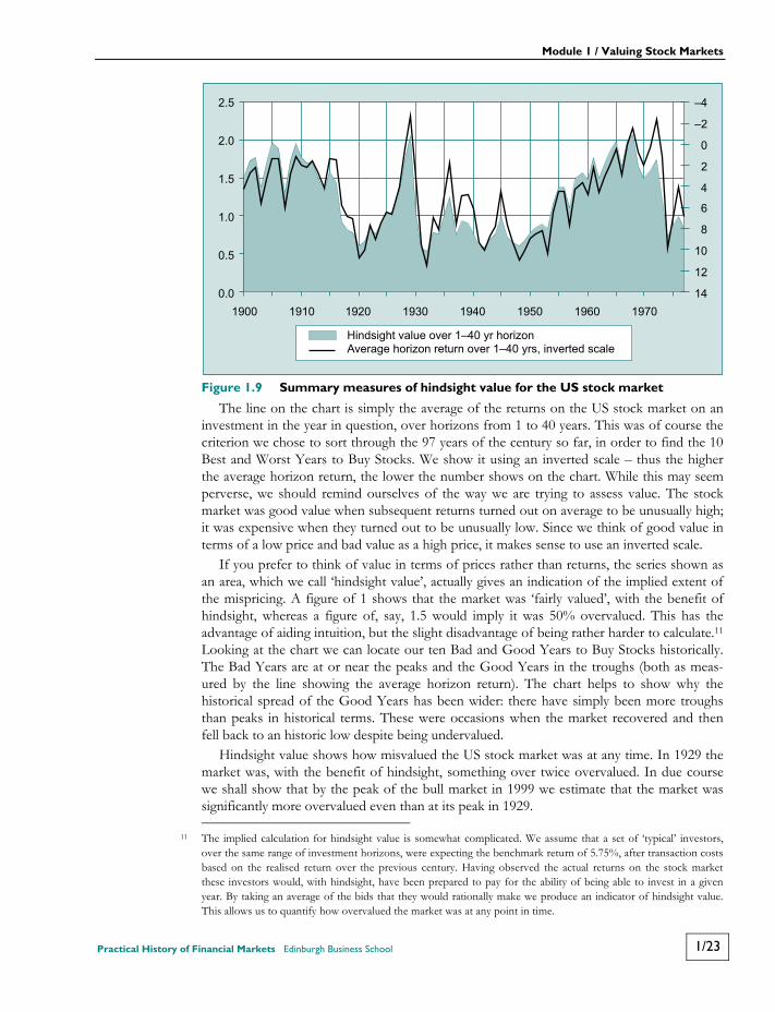
Module 1 / Valuing Stock Markets
Practical History of Financial Markets Edinburgh Business School 1/23
Figure 1.9 Summary measures of hindsight value for the US stock market
The line on the chart is simply the average of the returns on the US stock market on an investment in the year in question, over horizons from 1 to 40 years. This was of course the criterion we chose to sort through the 97 years of the century so far, in order to find the 10 Best and Worst Years to Buy Stocks. We show it using an inverted scale – thus the higher the average horizon return, the lower the number shows on the chart. While this may seem perverse, we should remind ourselves of the way we are trying to assess value. The stock market was good value when subsequent returns turned out on average to be unusually high; it was expensive when they turned out to be unusually low. Since we think of good value in terms of a low price and bad value as a high price, it makes sense to use an inverted scale.
If you prefer to think of value in terms of prices rather than returns, the series shown as an area, which we call ‘hindsight value’, actually gives an indication of the implied extent of the mispricing. A figure of 1 shows that the market was ‘fairly valued’, with the benefit of hindsight, whereas a figure of, say, 1.5 would imply it was 50% overvalued. This has the advantage of aiding intuition, but the slight disadvantage of being rather harder to calculate.11 Looking at the chart we can locate our ten Bad and Good Years to Buy Stocks historically. The Bad Years are at or near the peaks and the Good Years in the troughs (both as meas-ured by the line showing the average horizon return). The chart helps to show why the historical spread of the Good Years has been wider: there have simply been more troughs than peaks in historical terms. These were occasions when the market recovered and then fell back to an historic low despite being undervalued.
Hindsight value shows how misvalued the US stock market was at any time. In 1929 the market was, with the benefit of hindsight, something over twice overvalued. In due course we shall show that by the peak of the bull market in 1999 we estimate that the market was significantly more overvalued even than at its peak in 1929.
11 The implied calculation for hindsight value is somewhat complicated. We assume that a set of ‘typical’ investors, over the same range of investment horizons, were expecting the benchmark return of 5.75%, after transaction costs based on the realised return over the previous century. Having observed the actual returns on the stock market these investors would, with hindsight, have been prepared to pay for the ability of being able to invest in a given year. By taking an average of the bids that they would rationally make we produce an indicator of hindsight value. This allows us to quantify how overvalued the market was at any point in time.
0.0
0.5
1.0
1.5
2.0
2.5
1900 1910 1920 1930 1940 1950 1960 1970
–4
–2
0
2
4
6
8
10
12
14
Hindsight value over 1–40 yr horizonAverage horizon return over 1–40 yrs, inverted scale

Module 1 / Valuing Stock Markets
1/24 Edinburgh Business School Practical History of Financial Markets
Of course, while we can measure the degree of overvaluation in 1929 with the benefit of hindsight, when we look at more recent years this is clearly impossible. So we need now to approach the issue of value in a forward-looking sense. Before we do so, however, we need to address more seriously the view that attempting to do so is simply a waste of time.
1.6 But Can Markets be Valued? Efficient Markets, Random Walks, and the ‘Buy and Hold Strategy’
1.6.1 Taking Stock
We have now established two reasonably solid ‘stylised facts’ on the basis of the available data on the history of long-run stock returns.
First, in Section 1.4 we showed that, over sufficiently long periods, average realised stock returns seem to have been fairly stable, from which we can indirectly infer that, as long as expectational errors have not clouded the picture too much, the desired return of the typical investor has also been fairly constant.
Second, in Section 1.5 we established that, if this typical investor were to look back over the history of the US stock market, they would be able to clearly identify, with the bene-fit of hindsight, points in time when, given their desired return from investing in stocks, the stock market represented good or bad value. It was good value at points when sub-sequent returns at a range of horizons were very good, compared with normal; it was bad value when subsequent returns were relatively very poor.
Are these two features of the data sufficient evidence for us to assert that markets can be valued in a forward-looking sense, rather than just with the benefit of hindsight? The answer should, we hope be clear: No. They are not. In mathematical jargon, these two features are necessary conditions for us to be able to value markets, but they are not sufficient conditions.
There is a third condition that we need to satisfy if we are going to argue that markets can be valued. This condition is that a key prediction arising from the predominant theory about stock markets put forward by economists, the Efficient Markets Hypothesis, must be wrong. This must in turn imply that what was (at least until recently) the predominant theory about investment, the ‘Buy and Hold Strategy’, must also be wrong.
In this chapter we address this issue. We shall first summarise the key (and, it turns out, closely related) arguments of both the EMH and the Buy and Hold Strategy, and then go on to show that both theories are seriously undermined by that second remarkable feature of stock returns that we referred to at the start of Section 1.4: that stocks appear to have been ‘too safe’.
1.6.2 Efficient Markets and Random Walks
The Efficient Markets Hypothesis is very important. It almost, but not quite, represents the standard view of economists about the stock market. It says something extremely simple, which is that shares are always correctly priced. In a world of perfectly efficient markets, stock prices change only because new information becomes available. This new information changes prices, because it changes a rational assessment of the future. If this is correct, all information on which share prices depend is immediately taken into account by the market
Module 1 / Valuing Stock Markets
Practical History of Financial Markets Edinburgh Business School 1/25
as soon as it becomes known. No reassessment of historic information will change prices, only new information. In such a world there can be no deviation from ‘fair’ value, since financial markets arrive at prices that are always and everywhere automatically ‘fair’.
Note that the assertion that markets are efficient in this sense in no way implies that they can correctly predict the future. Even a notionally perfectly efficient market would make prediction errors. But the ‘fair’ value that it arrived at would be the best estimate that could be made given all the information at the time. When new information became available, however, market participants would reappraise this fair value, and markets might go either up or down: hence the assumption that efficient markets are driven only by information, by ‘news’.
It follows that, in an efficient market, value cannot be sensibly discussed, as the only sensible way to measure value is by looking at current stock prices. No valuation criterion is worth using, since the market price itself is the best valuation criterion and cannot be improved upon.
The Efficient Markets Hypothesis is a wonderfully simple and extremely powerful idea. Efficient markets are assumed to be efficient because, if someone finds a new way to predict movements in prices, this is, in effect, a money machine. Efficient markets abhor money machines, just as nature abhors a vacuum. In an efficient market, any money machine that may occur will immediately be exploited by other traders through arbitrage, so rapidly and so thoroughly, that the money machine must cease to be a money machine.
Like all the best simple ideas, the Efficient Markets Hypothesis can also be used to make clear predictions about how we would expect financial markets to work. These predictions can be tested. It is no surprise, since economists have to have something to do to occupy their time, that vast numbers of tests of the Efficient Markets Hypothesis have been carried out, on any imaginable market, in almost every part of the planet. Perhaps to the surprise of those who believe economists cannot come to conclusions, this work has led to some important areas of consensus.
One simple prediction that arose out of the Efficient Markets Hypothesis was the idea that stock prices should behave like a ‘random walk’. Testing for a random walk is just testing whether stock price changes are at all predictable. If they were, this would imply the existence of a money machine, which efficient markets would abhor.
It should be fairly evident that, in themselves, the two features of stock returns that we alluded to at the start of this chapter do not necessarily contradict the Random Walk Hypothesis.
If investors always simply got the return they expected, plus an entirely unpredictable element due to making incorrect (but still, in principle, rational) predictions about the future, we would still observe the first feature of an apparently stable Siegel's Constant, as long as the typical investor's desired return was stable.
We would also be able to identify good and bad years to have bought stocks after the event, but, crucially, only with the benefit of hindsight. By analogy, a gambler on a roulette wheel in a casino can always identify, after the event, the point when a good or bad run of luck started. But, since roulette wheels are truly random, such runs of good or bad luck can never be predicted in advance (despite all that the compulsive gambler will tell you!).
Thus, if the Random Walk Hypothesis were correct, our two features would be necessary but not sufficient conditions to be able to assess value in a forward-looking way.
Module 1 / Valuing Stock Markets
1/26 Edinburgh Business School Practical History of Financial Markets
However, it is now widely agreed amongst economists that the random walk version of the Efficient Markets Hypothesis is very nearly but, crucially, not quite supported by the data.
Over short time horizons, in well-developed markets, the theory works well. Over longer time horizons, even in well-developed markets, research shows that there are violations of the hypothesis. These violations are generally ‘statistically significant’, but, crucially, they are not in general of the order of magnitude that would make it worthwhile attempting to make money by exploiting them. We shall show some evidence that gives a graphic demonstration of this later in this section.12
1.6.3 The Buy and Hold Strategy
It may not be immediately obvious, but the Random Walk version of the EMH has a lot in common with what was, until recently, the predominant approach to investment: the Buy and Hold Strategy. 13 Both reject the idea that markets can be valued in any useful way.
The Buy and Hold Strategy asserts, in essence, that, in contrast to the evidence we pre-sented about historically good and bad years to buy stocks in the previous chapter, now is always a good time to be holding stocks.
The link with the EMH is that the logic of the Buy and Hold Strategy can only hold if returns are unpredictable. If there were any predictability in returns, this could be used to spot the bad times to buy stocks, thereby undermining the whole basis of the strategy. If this were not the case – if it were after all possible to spot a good time to get out of stocks – then you would not buy-and-hold, you would buy-and-sometimes-hold-but-sometimes-sell.
Understanding the intimate connection between the logic of the Buy and Hold Strategy and that of the Random Walk Hypothesis is very helpful.14 One of the great attractions of the random walk hypothesis is that it makes very clear predictions about the way returns will behave, which are therefore testable against real-world data. Any such test is therefore also implicitly a test of the logic of Buy and Hold. Both ideas have to face the puzzle we alluded to at the start of Section 1.5, which is that, according to their own logic, stocks have in practice been ‘too safe’ an investment.
12 For summaries of more sophisticated econometric approaches to the statistical evidence, see, e.g., Campbell, Lo and
MacKinlay (1996) The Econometrics of Financial Markets, Princeton University Press; Lo and Mackinlay (1999) A Non-Random Walk Down Wall Street, Princeton University Press; Cochrane, (2001) Asset Pricing, Princeton University Press. Note that amongst many financial economists (most of the above authors, for example) evidence against the random walk hypothesis has not been accepted as killing off the EMH. We briefly discuss the way that proponents of the EMH have assimilated the rejection of the random walk hypothesis in Section 1.14.
13 Probably the most effective and coherent proponent of this view is Jeremy Siegel (1994), in Stocks for the Long Run, McGraw Hill.
14 A more precise, but less catchy title for the Random Walk Hypothesis, as used here, would really be the Unpredictable Returns Hypothesis. Unpredictable returns would imply that the cumulative total return to stocks would be a random walk, rather than stock prices, as early versions of the Random Walk model assumed. But the contrast between the Random Walk theory as applied to stock prices and the assumption that returns are random is not in practice very great. Under the less restrictive unpredictable returns theory, since the dividend component in returns is fairly predictable over the short run, there must be an offsetting predictability in stock prices, such that total returns are random. In practice this would make the stock price very close to being a random walk.

Module 1 / Valuing Stock Markets
Practical History of Financial Markets Edinburgh Business School 1/27
1.6.4 The Puzzle: Have Stocks Been ‘Too Safe’?
Proponents of the Buy and Hold Strategy do not deny the short-run volatility of stock returns, but argue that the impact of such volatility is diminished by the averaging-out process of returns over long horizons that we saw in Figure 1.5 and Figure 1.6. There is indeed a clear basis in probability for this assumption. For example, Figure 1.5 showed that there is a 10% chance of the return in any one year being better than 30% or worse than minus 22%. If returns were completely random, the chances of the average return over two years being in that range would be only 1%. This is simply because the chances of a one in ten chance repeating itself two years running is ten times ten to one against. The result is that the risks to investors would diminish over time, even if returns were random.
In practice, however, the reduction in risks that would occur if returns were unpredictable cannot be used to justify the Buy and Hold Strategy. Not because it would not happen, but crucially, because it would not happen fast enough. Figure 1.10 illustrates why. It shows the difference in risks between investing in stocks in the real world and investing in them if returns were unpredictable, as both the Random Walk Hypothesis and the Buy and Hold Strategy must imply. Rather than looking at the average return we look at the variability in the lump sums that investors would have received. Looking at things in this way helps bring out the scale of the differences, since small differences in returns amount to a lot of money over 20 or more years.
Figure 1.10 Buy and Hold has been safer than its own logic would predict
For those who invested $1 in every single year over the past two centuries, the inner band in Figure 1.10 shows the range of amounts they would have been able to realise in real terms depending on how long they chose to hold the investments. The chart tells you that, 90% of the time, the lump sums they would have ended up with would have been somewhere in this range. Only 5% of the time would you have ended up with a higher lump sum and only 5% of the time with a lower one. Ending up with a lump sum less than one implies that investors lost money in real terms and the chart shows that, at a 14-year horizon, this happened only 5% of the time. They therefore had a 95% probability of getting at least some
Re
al va
lue
of
$1
in
ve
ste
d a
t sta
rto
f p
erio
d w
ith
re
inve
ste
dd
ivid
en
ds
0
1
10
100
10 20 30
Number of years you stay in stocks
If stock returns were random, as the Buy and Hold strategy mustimply, returns on lump sums invested in stocks, over differenthorizons, should lie in this range 90% of the time. So you would needto wait 30 years to reduce the chance of losing money to 5%.
But actual returns have stayed within this significantlynarrower range: real investors have only needed to wait14 years to reduce the chance of losing money to 5%.
Log scale
Module 1 / Valuing Stock Markets
1/28 Edinburgh Business School Practical History of Financial Markets
sort of positive return if they waited this long. (We shall see in Section 1.11 that over a 20-year horizon this has been the case in practice all the time.)
The outer band on the chart shows the range of variation that would occur if the logic of the Buy and Hold Strategy were sound. The difference is very marked indeed. Had returns been entirely random, you would have needed to wait over 30 years to have a 95% probabil-ity of getting at least some positive return.
This says something extremely important about the Buy and Hold Strategy. If the logic of the strategy were correct, stocks would be far riskier than they actually have been.15 They would arguably be simply far too risky, even for the very long-run investor. But the very success of the Buy and Hold investment strategy therefore undermines its own logic. The Buy and Hold Strategy cannot explain its own success.
It also, clearly, says something important about the EMH, at least in its straightforward Random Walk version. Returns cannot have been entirely unpredictable in the past because, if they had been, stocks would have been far more risky than they actually have been.
1.6.5 Necessary and Sufficient Conditions
The rejection of the Random Walk version of the EMH, and the associated rejection of the Buy and Hold Strategy, is crucial. There is some degree of predictability of stock markets.16 By implication, we have established necessary and sufficient conditions to be able, in principle, to value markets. We shall now turn to the practicalities of doing so.
We should perhaps stress at this stage that the ability to value stock markets may reject the strictest version of the EMH, but it is not in principle inconsistent with a more limited definition of efficiency. Nor does it imply that market participants are necessarily irrational. We shall hope to convince you that it is usually possible to tell whether markets are over- or undervalued, but this information cannot be used to make big profits without taking big risks. Most of the time, when markets are neither extremely over- nor undervalued, value is not very important, since it cannot be used to make strong predictions about future returns. It is only in times of extremes that knowing about value can provide vital information. But, as the experience of the 1990s showed, those can be exactly the times when, for investment professionals, at least, acting on that information can be very risky indeed (an issue we shall discuss at greater length in Section 1.14).
15 Our arguments here about the significance of the difference between the outer and inner bands are quite informal.
For a more formal investigation of this, which establishes that they are indeed different in a statistically significant sense, see Donald Robertson and Stephen Wright's working paper, ‘The good news and the bad news about long-run stock returns’ (www.bbk.ac.uk/faculty/wright)
16 Without undue immodesty, we should point out that this is not just something that we can say with hindsight. Our book Valuing Wall Street was written during the last year or so of the 1990s boom, and predicted the collapse of the US stock market well in advance of the peak. Nor were we the only people to make such predictions (though, clearly, we were in a minority amongst investors).
Module 1 / Valuing Stock Markets
Practical History of Financial Markets Edinburgh Business School 1/29
Indicators of Stock Market Value
1.7 Five Key Tests for a Useful Measure of Value We shall now propose a number of tests that must be satisfied if a measure of value is to be a valid and useful concept. We shall first examine the basis for these tests, before we proceed to apply them to alternative indicators of value.
Test No. 1 An indicator of value must be measurable This test may seem so basic as to be hardly be worth mentioning, if it were not so
important. Value must be measurable. To claim that the market is wrongly priced can make sense only if it would be correctly priced at some other level, which is typically referred to as fundamental value, or just the fundamental. When the market is correctly, or ‘fairly’ valued, price and fundamental value will be the same. When they are not, the ratio between the two will show the extent to which the market is over- or undervalued. Clearly, in order to arrive at this ratio, the fundamental value must be measurable.
Some aspects of this issue are merely superficial. Confusions can sometimes arise, for example, because different approaches to value put the relevant ratio a different way up. Thus we shall see that, while, for example, q and the price-earnings multiple both put price on the top of the ratio, with the fundamental at the bottom, the dividend yield puts price on the bottom of the ratio. When the market is overvalued, q will therefore be high, but the dividend yield will normally be low. The degree of implied overvaluation can, however, be compared by turning the dividend yield upside down.
But there are also much deeper problems of measurability that apply to all indicators. Profits, for example, which feed into the P/E multiple, can include significant distortions. Less obviously, we shall see that there are major problems in measuring ‘true’ dividends, now that companies so frequently find other ways of returning cash to shareholders. q, our preferred measure, defined below, depends on corporate net worth, which is also something that cannot be measured perfectly.17At this stage, however, we shall merely state that we do not think that such objections can be reasonably maintained. When we examine any potential valuation measure, we must pay close attention to such measurement issues.
Test No. 2. The resulting ratio of price to fundamental value must mean-revert The statistical feature of mean reversion is crucial to any indicator of value. Mean
reversion implies that the ratio between the stock price and the fundamental value of the market is pulled back towards its average like a piece of elastic: it must therefore have a tendency to ‘revert’ to its ‘mean’.
It's worth considering this aspect of value a little more thoroughly, since it is so crucial to our arguments. The best way to illustrate is with concrete examples. Figure 1.11 and Figure 1.12 show the difference between two valuation indicators, using a century of data, one of which definitely mean-reverts, and one of which definitely does not. We happen to
17 We shall see in due course that the measurement problem is probably the only intellectually coherent objection to
q.
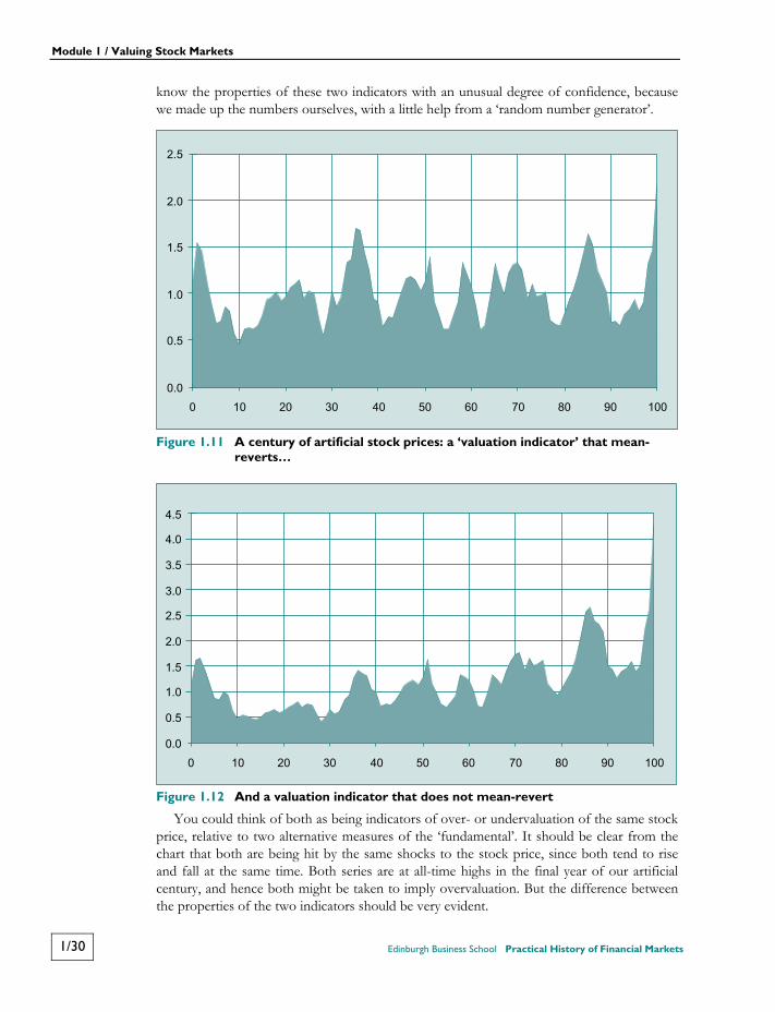
Module 1 / Valuing Stock Markets
1/30 Edinburgh Business School Practical History of Financial Markets
know the properties of these two indicators with an unusual degree of confidence, because we made up the numbers ourselves, with a little help from a ‘random number generator’.
Figure 1.11 A century of artificial stock prices: a ‘valuation indicator’ that mean-
reverts…
Figure 1.12 And a valuation indicator that does not mean-revert
You could think of both as being indicators of over- or undervaluation of the same stock price, relative to two alternative measures of the ‘fundamental’. It should be clear from the chart that both are being hit by the same shocks to the stock price, since both tend to rise and fall at the same time. Both series are at all-time highs in the final year of our artificial century, and hence both might be taken to imply overvaluation. But the difference between the properties of the two indicators should be very evident.
0.0
0.5
1.0
1.5
2.0
2.5
0 10 20 30 40 50 60 70 80 90 100
0.0
0.5
1.0
1.5
2.0
2.5
3.0
3.5
4.0
4.5
0 10 20 30 40 50 60 70 80 90 100

Module 1 / Valuing Stock Markets
Practical History of Financial Markets Edinburgh Business School 1/31
The first regularly gets pulled back from extreme values – whether high or low – towards its mean. In terms of the language made fashionable by chaos theory, its average value is an attractor. This means that the final value really is ‘high’, implying that there is a high probability that it will fall back.
The second indicator, in contrast, has no such tendency. Whether it is low or high, there is an equal probability that it will fall or rise – history simply does not matter. Like any series that does not mean-revert, the best guess you can make about its own future is usually that it will stay at or near its current level.18 For a series like this, the words ‘high’ or ‘low’ have no meaning, since they cannot be made in comparison with a stable mean. Such a series cannot have anything useful to say about stock market value.
The mean-reverting ratio is different. The fact that it mean-reverts implies that the stock price cannot deviate too far from its fundamental without the elastic beginning to tug. Such an indicator therefore has information about our artificial stock market's future.
A crucial feature of mean reversion is, however, the element of uncertainty. We know the properties of the mean-reverting indicator in Figure 1.11, because we constructed it ourselves. Nonetheless we cannot know exactly what would happen in the first year of our next century of artificial data. The precise outcome would depend on the element of ‘noise’ injected by our random number generator. Although the indicator is at an all-time high, we cannot rule out that this element of ‘noise’ might push it even higher. All we can say is that there is a rather low probability that this will actually happen.
When we come to look at real as opposed to artificial stock markets, this element of uncertainty is both a necessity and a nuisance.
It is a necessity, because without uncertainty it would be too easy to make money by exploiting indicators of value. We shall see that uncertainty about mean reversion is a necessary condition for any valid indicator of value.
But uncertainty is also a nuisance. Since we constructed the data for the two charts our-selves, we have no difficulty in knowing which of the two indicators genuinely mean-reverts. This is not always so easy when you are dealing with real stock markets. We can use statistical tests to establish whether possible indicators of value exhibit this crucial property. We shall restrict our discussions here to looking at the properties visible in charts, but shall refer to more formal statistical tests that have been carried out in academic papers. As it happens, the two approaches are mutually supportive, but statistical tests help to guard against what is perhaps an innate human tendency to spot patterns that are not really there. Rigorous testing injects a greater element of objectivity.
Unfortunately, data analysis in isolation cannot tell you everything. A major problem in economics, as in any science that cannot run controlled experiments, is that if you go out looking for statistical evidence in favour of your own views, and are prepared to look both hard enough and selectively enough, you may well find some data, somewhere, to bolster your case. If you do this, you run a severe risk of what economists call data mining. The analogy should be quite clear. If you were a mineral prospector who used all the tricks of your trade to track down and mine a seam of gold, you would not conclude from this that gold is everywhere beneath our feet. The very activity of mining shows that the thing being mined is rare. The same applies to statistical evidence. The harder you have to search to find it, the less useful it is as evidence.
18 The simplest example of a series with this property is usually referred to as a random walk.

Module 1 / Valuing Stock Markets
1/32 Edinburgh Business School Practical History of Financial Markets
You should always be on your guard against evidence that is merely the result of data mining. There are two very important ways to guard against it.
The first is to use all available data, without being selective. We have at least a hundred years of data on most of the indicators of value we discuss, and we use it all. If we had more we would use that as well. Nonetheless, it is very rare to see such large amounts of data used. Being charitable, this may of course be due to ignorance or laziness. Or perhaps we should say‘ being relatively charitable’, as the alternative to ignorance and laziness is a wilful intent to deceive. But when we come to look at other indicators of value and, in particular, yield ratios and yield differences, we shall see that the only empirical support for them depends on a selective use of data and hence on data mining. If all available data are used, the appearance of statistical evidence dissolves like the phantom that it is.
There is a second very crucial way to guard against data mining; but it is much more than just this. It is so important that we deal with it separately in our next test.
Test No. 3. An indicator of value must make economic sense. Value must have a firm basis in terms of economics. This means that how it works must
be understandable. This is not only because the search for understanding is the basic drive behind economics or any other science, though this is important. All theories need to stand up to argument, because this is an important way in which they are tested. If they are robust they are confirmed by debate, but if a better theory comes along then they are discarded. Testing and prediction are important parts of this process, but they are not the only ways in which one theory is preferred to another. The ability to enlighten is crucial.
An understandable theoretical basis provides a key protection against data mining and the human tendency to see patterns that are not really there, which we discussed in relation to the issue of mean reversion. If we start from a theory and then test it, there is always a chance that the data will fail to reject that theory merely by accident, though if we had had more data our theory would have failed the tests. But when we find that the data do not reject a theory that illuminates our understanding, we have far less risk of data mining by accident. The more data we have, the more confidence we can have in the theory. But all data are limited and a theory that is designed to explain an apparent pattern is far more likely to prove illusory, than a theory that is first propounded because it enlarges our understand-ing and is then successfully tested against the evidence.
Test No. 4. An indicator of value must tell you something (but not too much) about future stock returns. We saw in Section 1.6 that a crucial piece of evidence against textbook efficient markets
is that stock markets are not quite a random walk. Figure 1.10 showed that, if they were, stock returns would be far riskier, over long horizons, than they actually have been historically. By implication, there is some degree of predictability in stock returns. To be useful, a valid indicator of value must help predict future returns.
You should, however, be deeply sceptical of any indicator of value that is alleged to provide more than a very minimal amount of predictive power for future returns. The necessity for not saying too much is perhaps disappointing, but it provides an important reality check. If movements in stock prices, especially over the short-term, could be predicted, it would be too easy to make money by exploiting indicators of value. We cannot expect people not to make
Module 1 / Valuing Stock Markets
Practical History of Financial Markets Edinburgh Business School 1/33
money if they are offered the opportunity to do so without risk. There must therefore be sufficient risk to deter them from making money through arbitrage. When price and funda-mental value diverge, market participants should be capable of knowing that they have and indeed of measuring by how much, at least to within some margin of error. But they should not be able to profit from this knowledge without some form of risk.
It is this uncertainty that has given rise to most of the misunderstandings that surround any discussion of stock market value. We are simply innocent economists trying to under-stand things. We don't expect to be able to make much money from the understanding we hope to achieve from our efforts. This makes us sharply different from most other people who look at value. They are usually practical people, who wish to make money, either by buying and selling shares or by persuading others to do so. For the most part, we see nothing wrong in such attempts. We are not taking a moral stance. Our scepticism regarding attempts to time stock markets is simply that, innocent as we are, we are not perhaps innocent enough, and consider such attempts to be naïve. The naïveté consists in expecting to be able to forecast the timing with which stock markets will move, at least with sufficient accuracy to make money out of it. This is the same as expecting people not to pick up hundred dollar bills.
This inability to predict when things will happen, but not what will happen, can be illus-trated again by the example of a roulette game. The chances of winning at roulette are not quite even, owing to the existence of zero. The result is that, on average, the ‘house’ always wins and the punters always lose. But this does not mean that any individual is bound to lose during the course of an evening's play. If it did then roulette would be unlikely to draw the crowds it does. A punter should know that he is bound to lose if he plays for long enough, but you cannot predict when this will happen. What you do know is that the chances of losing rise, the longer the game is played.
A valid criterion of fundamental value will put the investor in a similar position to the ‘house’ at roulette. The stock market is as competitive as it gets, and we can thus be sure that, while any valid criterion of value must mean-revert, there must be considerable uncertainty about when this will happen. The uncertainty about timing must be large. The profits from correctly judging market fluctuations are huge. The risks over timing must be equally great, or the returns from arbitraging the market would not balance the risks of doing so.
The risks associated with predicting future returns, and attempting to make an arbitrage profit therefrom, explain why our approach differs from the textbook version of the Efficient Markets Hypothesis. Under the EMH, arbitrage is assumed to be so rapid, and so complete, that price cannot depart from fair value. If arbitrage is risky it can. But in consequence, if the EMH is not to hold, arbitrage must be risky: hence the predictive power associated with a valid valuation criterion must be weak.
Test No. 5. The fundamental must be relatively stable. Our final test requires a rather basic, but crucial, feature. The more stable the funda-
mental, the more useful will its ratio to price be as a criterion of value. A highly volatile fundamental would render the ratio of price to fundamental almost useless, since the ratio would be continually jumping around as a result of changes in the fundamental, rather than in price. Stability of the fundamental has the added advantage, in terms of common-sense intuition, that in general the stock market will get more expensive when the stock price rises, and cheaper when it falls.
Module 1 / Valuing Stock Markets
1/34 Edinburgh Business School Practical History of Financial Markets
Another way to look at this test is that mean reversion of the valuation indicator, required by our second test, must be driven primarily by changes in price, rather than by changes in the fundamentals. Economic theory may predict that the ratio will mean-revert (as our third test requires) but be uncertain as to how this will occur. A high value of the ratio might, for example, tell us only that there is a high probability that the fundamental is going to rise, rather than that the price is going to fall. If this were the case, we would be able to use the valuation indictor to predict changes in the fundamental, but not changes in the stock market.
Even our fourth test, that an indicator of value should have some weak predictive power for returns, is of limited use if the value of the fundamental itself is very hard to predict. It may possibly have some short-term predictive value, but, unless we can have an expectation that the fundamental itself will be reasonably stable, and hence, from mean reversion, that the stock market will be pulled back towards this stable value, this will not be much help over the sort of longer horizons that are usually of interest to investors in the stock market.
1.7.1 A Cross-Check: Valid Approaches to Value Must Be Mutually Supportive
A crucial cross-check of our five tests is that, if we regard any valuation criterion as valid, it should be consistent with any other criterion we regard as valid. This point should be fairly obvious in logic. If there were absolutely no uncertainties about data, like those discussed above, then we might in theory be able to arrive at some ‘ideal’ valuation criterion. Any such criterion must also logically be unique. Actual valuation criteria using real data must always be imperfect images of this true ideal measure. As such, they will not always agree. But, when they disagree, we should be able to understand the source of this disagreement. We shall have more to say about this in Section 1.14.
1.7.2 Valid and Invalid Measures of Stock Market Value
In the next six sections, we shall now consider the various ways of valuing stock markets that have, from time to time, been proposed, and see whether they satisfy our five criteria. The measures we shall consider are the dividend yield, P/E ratios (both unadjusted and cyclically adjusted), bond/yield ratios, and q. There are no doubt some others we could consider, but these are the measures that are most usually discussed, and include the two valid criteria, q and cyclically adjusted P/Es; an important, but flawed measure, the dividend yield; and the most commonly used, but invalid approach, the bond/yield ratio. In each case we shall show, in separate boxes, how the claims made for each indicator as a measure of value can be related to the Dividend Discount Model, as set out in Box 1.1, in Section 1.3.
The two valid measures, q and the cyclically adjusted P/E, are each derived from one of the two basics set out earlier. q follows from the fact that equities represent a title to the ownership of real assets, while the cyclically adjusted P/E follows from the fact that equities are financial assets.
Either approach may therefore in theory, though not necessarily in practice, provide a valid measure of value.
Either approach may of course be misused to produce invalid measures. But, if they prove practical and are correctly used, they must give the same answer.

Module 1 / Valuing Stock Markets
Practical History of Financial Markets Edinburgh Business School 1/35
Valuing the stock market using q, by defining the fundamental from the necessary equi-librium of stock market value with the replacement cost of companies, to which share ownership provides the title, is relatively straightforward. Although, as we shall see, it has been misused, this has been relatively rare. We shall discuss the use of q for the US, UK and Japanese stock markets. Unfortunately, in most other markets, the data required to measure q are often not available.
Valuing the stream of income at the correct discount rate is more complex. The key problem, which is ignored with alarming persistence, is that the current level and growth of income in the future determine the correct rate at which their value should be discounted. In standard economic terminology, the income stream and the discount rate are not exogenous, but endogenous. The cyclically adjusted P/E provides a valid solution to this problem if we are prepared to make one key assumption about the nature of the discount rate to be applied. The dividend yield has more serious flaws. The bond yield ratio is entirely invalid.
1.7.3 Conclusions: A Summary of the Five Key Tests
To summarise, our five tests for any valid indicator of value are:
1. An indicator of value must be measurable. 2. The resulting ratio of price to ‘fundamental value’ must mean-revert. 3. An indicator of value must make economic sense. 4. An indicator of value must tell you something (but not too much) about future stock
returns. 5. The fundamental must be relatively stable.
A necessary corollary of these tests, as we shall see, is that valid indicators of value must be mutually supportive.
1.8 The Dividend Yield
1.8.1 Basics
The valuation criterion with the longest history is the dividend yield. It is calculated by dividing the annual dividend on a share by its current price, expressed as a percentage. The dividend yield for a stock market index such as the Dow Jones Industrials, or the S&P 500, is an average of the dividend yields on the individual stocks in the index.
The dividend yield can be very informative, whether or not it can be used as a guide to value. For example, the very low dividend yields of recent years provided two key items of infor-mation. One was that income alone could not justify an investment in stocks, since for much of the boom cash on deposit gave a better income than dividends. The second, which relates to our discussion of stock market value in Section 1.3, was the necessary implication that anyone holding stocks despite these low dividend yields must rationally have been expecting capital gains (and hence definitely not the capital losses they actually received over this period).
While these two items are useful bits of information they cannot be used to tell you anything directly about value.
It is also clear that the dividend yield provides very little guide at all to value when you look at individual shares. Many companies, particularly smaller ones, pay no dividends, and this does not make them valueless, provided there is a reasonable expectation that they will start to pay dividends at some point in the future.

Module 1 / Valuing Stock Markets
1/36 Edinburgh Business School Practical History of Financial Markets
It is only when the average dividend yield on the whole stock market is being considered that the possibility of using it as a guide to value can be reasonably considered. The dividend yield is not unique in this respect. The difference between trying to value individual shares and valuing the stock market as a whole is something that is common to all valuation criteria. It is common, unfortunately, to find that this important distinction is often poorly understood.
Test No. 1. Does the dividend yield provide a measurable indicator of value? At first sight the answer to this question must obviously be ‘yes’. One of the great
advantages of the dividend yield is that both of the two elements of which it is made up – the price, and dividends per share – are measured very precisely, and the data are readily available. If you are so inclined, you can keep tabs on the dividend yield on individual stocks, and on market indices, on an almost minute-by-minute basis.
Reliability of the underlying data is one of the great pluses of the dividend yield. But being 100% confident of the top and bottom of the ratio between dividends per share and the share price is not the same thing as saying it is measurable as an indicator of value. We saw in the previous chapter that a measurable indicator must be able to tell us by how much the market is over- or undervalued at any time. The dividend yield does not do this. Its use involves the implicit assumption that there is some level of the dividend yield that corre-sponds to ‘fair’ value. Measurability is therefore a problem. It is not a problem of measuring the actual yield, but of measuring what the yield should be for the market to be at fair value. We discuss these issues in more detail in Box 1.2, and show both how they can be related to the Dividend Discount Model, and the problems that arise in this approach.
A common assumption is that the appropriate value to use is the historic average divi-dend yield, which is roughly 5.5%. At the peak of the market in 1999, the dividend yield was around 1%, implying, on the face of it, that the US stock market was some five and a half times overvalued. Even to us, at the time, this seemed a bit over the top. It is thus clear that, although there are no problems with the underlying data for the dividend yield, there are significant problems about knowing the correct average with which it should be compared.
Test No. 2. Does the dividend yield mean-revert? Figure 1.13 shows the dividend yield as far back as we have data, alongside its average
value. It suggests that the yield does not wander off indefinitely, but stays within bounds. By definition, it cannot fall below zero, and it has rarely approached double figures. But it is doubtful if it reverts to a mean. This doubt can be justified by statistical tests,19 but the evidence is visible to the naked eye.
19 See, for example, the ‘virtual appendix’ to Valuing Wall Street (www.valuingwallstreet.com). A recent academic study
coming to similar conclusions is Goyal A and Welch I, ‘Predicting the equity premium with dividend ratios’, NBER Working Paper 8788, 2002.

Module 1 / Valuing Stock Markets
Practical History of Financial Markets Edinburgh Business School 1/37
Figure 1.13 The dividend yield, 1871–2010
Data source Shiller (2000).
One simple check is to see how often the dividend yield crosses the line of its average value. A mean-reverting series should do this more often than the dividend yield does. Another common-sense test is to see whether it indicates that the stock market spends roughly as much time being overvalued as it does being undervalued, and that this pattern is reasonably consistent over different periods. The dividend yield clearly doesn't do this. It suggests that the market was nearly always undervalued in the nineteenth century and nearly always overvalued in the past 50 years. This simply contradicts common-sense.
To avoid this problem it is common to find that comparisons are made, not with the historic average derived from all the available data, but using only more recent information. Sometimes comparisons are made with the average over the twentieth century, which is lower than over both centuries, and sometimes only the last 50 years are used, which makes the average lower still. Another approach is to fit a trend, so that the ‘fair’ yield falls over time. These techniques simply cloud the issue, as there is no logical justification for any of them. They underline why mean reversion is such an essential property.
They also offer endless opportunities for data mining. If someone wishes to show that the market is overvalued they can simply compare the recent dividend yield with a long-term average. If they want to show that it is cheap, they can choose a much shorter period, and point out that the current yield is above its three-year or three-month average. The crucial point is that, without evidence of mean reversion, it is impossible to say that any claim based on the dividend yield is incorrect.
We must therefore conclude that, since the dividend yield fails the test of mean reversion, it fails altogether.
1871 1881 1891 1901 1911 1921 1931
1931
1941 1951 1961 1971 1981 1991 2001
Div
idend y
ield
Average 4.14%At end 2010 1.83%
14
12
10
8
6
4
2
0
14
12
10
8
6
4
2
0
Module 1 / Valuing Stock Markets
1/38 Edinburgh Business School Practical History of Financial Markets
Box 1.2: The Dividend Yield, ‘Fair Value’, and the Dividend Discount Model __________________________________________________ We saw in Box 1.1 that we can write the equalisation of the investors desired and expected returns as
1
where the first version is written in terms of the expected dividend next year, and the second is in terms of the current dividend yield, which we can measure. Let's imagine a world where the stock market was fairly valued, and investor's expectations were fulfilled (this is strictly hypothetical, but we can certainly imagine that this situation should at least hold on average). Then we can write this ‘equilibrium’ version of the formula (where the ‘hats‘ indicate an equilibrium value) as
1
which we can in turn rearrange as
So in a fairly valued market the dividend yield should be roughly equal to the investor's desired return, less the expected growth rate of dividends. By subtracting this expres-sion from the same expression in terms of the current dividend yield, we can write
so if the current dividend yield is, for example, below the value associated with ‘fair’ value, it must imply either that investors should expect returns to be lower than normal (the market is overvalued, if you are expecting the normal rate of return), or that growth of dividends per share must be expected to be higher than normal.
If we want to use the dividend yield as a valuation indicator, we thus have to be able to assume that the growth rate of dividends per share is more or less given, and then identify the level of the dividend yield associated with ‘fair’ value. We can then attempt to measure the degree of overvaluation by
//
where the ‘fundamental’ is current dividends, multiplied by the ‘fair’ ratio of prices to dividends (the ‘fair’ dividend yield turned upside down).
In practice, this presents major practical problems. Quite apart from the fact that we need to assume that e remains constant, it is also quite possible for the dividend yield to shift permanently downwards; but in this case the growth rate of dividends per share can normally not be taken as given, since, if companies continue to earn profits at the same underlying rate, the lower the payout ratio, the more they can plough back into the business, thus raising G. We shall look into this in more detail in Box 1.3 in Section 1.10. __________________________________________________________________________________________________________________________________________________________________________________________________________________________________________________________________________________________________________________________________________________________________________________________________________________________________________________________________________________________________________________________________________________________________________________________________________________________________________________________________________________________
Module 1 / Valuing Stock Markets
Practical History of Financial Markets Edinburgh Business School 1/39
Test No. 3. Does the dividend yield make economic sense as an indicator of value? The answer to this question is a pretty unambiguous ‘No’. As the box shows, investors
can in principle still get decent returns with a low dividend yield, as long as they can expect higher capital appreciation. Taking the historic average value of the dividend yield as indicating ‘fair’ value is entirely arbitrary. The fundamental problem is that any level of the dividend yield can in principle be consistent with fair value.
This is not just a theoretical possibility, but a very real one. We have already discussed, in Section 1.4, the remarkably historical stability of the real return on stocks, which we have dubbed ‘Siegel's Constant’. This has remained stable, over time, despite the historic tendency for the dividend yield to fall, so evident in Figure 1.13, because the lower income has been balanced by greater capital appreciation.
There is some evidence that lower dividend yields could be a sustained phenomenon. In the latter half of the twentieth century firms typically paid out lower dividends in relation to their profits than they did before. As we shall see in Box 1.3 (in Section 1.10), undistributed profits, which are those not paid out in dividends, increase companies’ net worth, and this increases their ability to pay additional dividends in the future. The more companies retain, the lower their current dividends per share, but the faster they can grow dividends per share in the future. Because the value of a share is made up of both current dividends per share and their ability to grow in the future, we cannot say that low dividend yields are necessarily a sign of an overval-ued stock market, let alone use them to say by how much it is overvalued.
We shall discuss one possible modification to the dividend yield at the end of this chap-ter; unfortunately, while this resolves some problems, it introduces new ones.
Whether payout ratios have or have not changed, and whether they have changed enough, are thus crucial questions that need to be considered before the dividend yield can be used to measure value. Neither point, however, is at all easy to establish.
In principle we could stop considering the dividend yield at this point. It fails to pass two of our five tests, and a valid criterion of value must qualify on all counts. However, for completeness, we consider the last two tests as well.
Test No. 4. Does the dividend yield tell you anything about future stock returns? In Section 1.6 we introduced the idea of hindsight value, which measured value in any
year in terms of the returns that were subsequently realised. Hindsight value is useless for today's stock prices, since we cannot apply hindsight to the future. But it is a very useful way to look at history, since we can compare it with the indicators that could have been measured at the time. If they show a strong relation with hindsight value, this must be because they could have told you something at the time about future stock returns.20
Figure 1.14 shows the performance of what we call dividend value. Normally dividends are used to value the market by use of the dividend yield, which measures dividends per share, divided by the price. A purely presentational difficulty with this measure is that, in contrast to, for example, q and the P/E multiple, the dividend yield shows the market as
20 More formal statistical tests of the dividend yield also produce very similar results. See, for example, the paper by
Goyal and Welch (op cit); also Donald Robertson and Stephen Wright ‘Dividends, total cashflows to shareholders and predictive return regressions’ (www.econ.bbk.ac.uk/faculty/wright).

Module 1 / Valuing Stock Markets
1/40 Edinburgh Business School Practical History of Financial Markets
cheap when the yield is high, and expensive when the yield is low. Our measure of dividend value deals with this presentational problem by turning the dividend yield upside down, to give the ratio of the stock price to dividends per share, and then compares the resulting value with its historic average.
Figure 1.14 ‘Dividend value’ and hindsight value
Figure 1.14 shows that the dividend yield actually does better on this test than in the previous two. High levels of dividend value, and hence low levels of the dividend yield, have frequently been associated with high figures for hindsight value, which means that subse-quent returns were below average. So the dividend yield has acted to some extent as a useful ‘leading indicator’ of lower returns in the future.
However, the usefulness of these signals is severely limited by the fact that the dividend yield fails the mean reversion test. The downward drift in the dividend yield meant that the market nearly always seemed cheap until the 1950s (even at the peak in August 1929) and nearly always seemed expensive after that. This was reflected neither in uniformly better returns in the earlier period, nor in uniformly worse returns afterwards. So, although the dividend yield seems to give useful warning signals, the magnitude of the signal does not indicate the magnitude of the risk. It is like an unreliable smoke alarm that may sometimes be going off in response to a major fire, or sometimes because a visitor has been imprudent enough to light a cigarette.
Test No. 5. Is the ‘fundamental’ for dividends relatively stable? As in the fourth test, the dividend yield does not do so badly on this last test as it did on
the first three. Dividends have typically been fairly stable. Figure 1.14 shows that, as a result, dividend value is a reasonable indicator of what is happening to value in the short-term. Its problems arise over the longer term, owing to its failure of mean reversion.
0.0
0.5
1.0
1.5
2.0
2.5
3.0
1900 1910 1920 1930 1940 1950 1960 1970
Hindsight value over 1–40 year horizon
‘Dividend value’
‘Dividend value’ turns the dividend yield upside down,to make it comparable to and the P/E.q

Module 1 / Valuing Stock Markets
Practical History of Financial Markets Edinburgh Business School 1/41
1.8.2 Conclusions: The Dividend Yield as an Indicator of Stock Market Value
Table 1.1 summarises the performance of the dividend yield in relation to our five tests. The table makes it clear that the dividend yield has severe defects. It can provide useful infor-mation, but as an indicator of value the dividend yield is deeply flawed.
The key problem with the dividend yield is that there is no basis in economics or statisti-cal evidence for the assumption that the dividend yield should have a stable average value, because companies can change their dividend payout ratios on a sustained basis without affecting returns to shareholders. Because it falls down on both Tests 2 and 3, it also fails on Test 1, and is unreliable on the last two tests.
Table 1.1 The dividend yield and the five key tests for any indicator of value 1. Measurability? Data reliable, but average unmeasurable.
2. Mean reversion? No.
3. Makes economic sense? No.
4. Weakly predicts returns? Yes, but signal is inaccurate.
5. Stable fundamental? Yes.
1.9 Redefining Dividends
1.9.1 Can the Dividend Yield be Salvaged as an Indicator of Value?
In the last section we saw that the major problem with the dividend yield is that there is no basis in economics or statistical evidence for the assumption that the dividend yield should have a stable average value, because companies can change their dividend payout ratios on a sustained basis without affecting returns to shareholders. Because it falls down on both Tests 2 and 3, it also fails on Test 1, and is unreliable on the last two tests.
Can the dividend yield be salvaged? One argument is that the change in the dividend payout ratio that has been evident in recent decades is more illusory than real. Since we have stated that dividends are very accurately measured, this may seem like a paradoxical statement. But it depends what you mean by dividends. We know the official definition of dividends, which is clear-cut. But there is an alternative, more functional definition. The economic function of dividends is to enable a transfer of cash from corporations to shareholders. But dividends, on a narrow definition, are not the only way that this transfer can be carried out.
It is worth stressing that, somehow or other, cash must always be transferred to sharehold-ers. If not, think about what would happen. We have seen already that the long-run average return on investing in stocks is around 6% in real terms. We shall show in due course that this must over the long-term be equal to the underlying return companies make. Suppose that companies did not return any cash to shareholders, but simply reinvested all profits at the same rate. This would imply that the underlying value of the corporate sector would also grow at a rate of 6% per annum in real terms. The underlying growth rate of most developed economies seems to be around 2–3% at best. If the corporate sector grew at 6%, in due course it would balloon out of all proportion to the rest of the economy, which is clearly unsustainable. For this reason, when we look at the rate of cash transfer of the corporate sector as a whole to shareholders, we know that, over the long-term, it must be pinned down by the difference between the rate of return of the corporate sector and the rate of growth of the economy. If
Module 1 / Valuing Stock Markets
1/42 Edinburgh Business School Practical History of Financial Markets
both of these are reasonably stable over long periods, then the rate of cash transfer – the ‘true’ payout ratio out of profits – must also be reasonably stable over long periods.
Since we have seen that recorded payout ratios in terms of standard dividends have fallen, if the overall rate of cash transfer is to be stable, the implication in logic must be that other forms of cash transfer must have taken the place of dividends. Reassuringly for economic logic, this is exactly what has happened.
There are three major alternative ways that the corporate sector can put cash into the hands of shareholders, apart from dividends.21
Probably the most well-known alternative is that companies can repurchase their own stock from shareholders. If a company buys back 1% of its shares at current market prices, this is exactly the same, in terms of cash transfer, as paying a dividend of 1%, but it is also typically much more tax-efficient (or at least was until recently). Repurchases have as a result grown enormously in recent years, to an aggregate level in the late 1990s not very different from standard dividends. Indeed, some companies at one stage made it a clear-cut policy that they would not pay old-fashioned dividends at all, but would dis-tribute cash solely by repurchases, if at all. Microsoft was probably the most celebrated example (although, interestingly, this announced policy was recently finally reversed by the payment of Microsoft's first ever dividend, albeit at a strictly cosmetic rate).
Less attention has been paid to what has been, in some years, of even greater quantitative importance as an alternative method of cash transfer: the impact of cash- or debt-financed mergers and acquisitions. As we pointed out in Section 1.3, when one company uses cash reserves, or issues debt, to buy up all the shares of another company, this is in effect a ‘terminal dividend’: the last ever payout that the original company will make. The net effect of this transaction is that the corporate sector as a whole has transferred cash to shareholders in just the same way as a conventional dividend. (Though note that, crucially, this is not the case if the acquiring company issues new equities to pay for its acquisition: in that case the total amount of equities of the two companies taken together does not change as a result of the acquisition.)
Finally, companies can also affect the aggregate amount of cash transferred to sharehold-ers by doing less of an activity that works in the opposite direction – namely, new issues. When a firm issues new equities it takes cash out of the hands of new or existing share-holders, so new issues are in effect dividends-in-reverse, when you look at the corporate sector as a whole. The data also show that, whereas in the early part of the twentieth century companies raised significant amounts of cash through new issues, thus offset-ting, in aggregate cashflow terms, the impact of what were then quite high dividend payments, this method of raising funds fell progressively out of favour over the course of the twentieth century.
Figure 1.15 shows the net effect, for the US non-financial corporate sector, of all these non-dividend forms of transferring cash to shareholders, by comparing the narrowly defined dividend yield to a broader ‘cashflow’ yield, that includes all alternative forms of cash payments.22
21 For an excellent survey of the data, and rationales for alternative, non-dividend transfers to shareholders, see Allen,
F and Michaely, R (2002), ‘Payout policy’, in George Constantinides, Milton Harris and Rene Stulz (eds) (2003)North-Holland Handbook of Economics in Finance, Corporate Finance Vol. 1A (Elsevier, Amsterdam).
22 The two yields are shown on a log scale to bring out the differences more clearly.

Module 1 / Valuing Stock Markets
Practical History of Financial Markets Edinburgh Business School 1/43
Figure 1.15 Alternative measures of US non-financial dividend yield
Data sources: Wright and Z1 tables B.102 and F.102.
The chart shows two key features, one of which is good news for the dividend yield as a valuation criterion; but the second is unfortunately distinctly bad news.
The good news is that the broader measure of the dividend yield, based on total cash-flows, does indeed appear to show greater stability, over long periods, than the narrowly defined dividend yield. In roughly the first half of the century, the ‘cashflow’ yield was typically less than the narrow definition, because new issues offset the impact of dividends; but as dividends fell out of favour, corporations offset the impact on total cashflow by using different combinations, at different times, of all three of the alternative methods described above. The visible evidence for mean reversion is supported by statistical tests; there is also reasonably strong evidence that the ‘cashflow dividend yield’ has predictive power for returns.23
Unfortunately, there is a quite a major piece of offsetting bad news. The chart also makes clear that, once we move to a more functionally based definition of dividends, which includes all forms of cashflow, the resulting yield series is far more volatile, in the short-term, than the conventional dividend yield. Since both measures are affected to the same extent by the rises and falls of the stock market, pretty much whenever the cashflow yield measures moves sharply, at a time when the standard measure does not, this is because there was a significant movement in total cashflow. Since total cashflow is the ‘fundamental’ for this alternative measure, this means that it is very volatile indeed, and that the cashflow dividend yield falls down very badly, as a consequence, on Test 5.
To see a very practical, and timely, example look at the last few years of data in Fig-ure 1.15. The conventional dividend yield over this period first fell quite sharply, and then went into reverse. Neither of these movements had much to do with the fundamental,
23 For evidence on both scores, see Robertson and Wright (op cit). So if we used this measure, we would do better on
at least tests 2, 3 and 4, than with the narrow measure.
10
9
8
7
6
5
4
3
2
1
0
10
9
8
7
6
5
4
3
2
1
01900 1909 1918 1927 1936 1945 1954 1963 1972 1981 1990 1999 2008
Cash flow yield Dividend yield

Module 1 / Valuing Stock Markets
1/44 Edinburgh Business School Practical History of Financial Markets
conventional dividends, but were almost entirely dominated by the rise of the market in the 1990s boom, and the subsequent bear market at the turn of the millennium. But note that the same pattern is entirely absent in the adjusted ‘cashflow’ dividend yield. The explanation is that, during the boom, total cashflow to shareholders rose every bit as fast as the stock market (indeed, in some years distinctly faster); but then collapsed just as fast in the bear market. As a result, at the peak of the market in the 1990s, the cashflow dividend yield gave almost no indication of the risk of poor returns.
It is perfectly possible that the rise in cashflow to shareholders in the 1990s is an im-portant part of the explanation of the boom. It was however clearly not a justification, since the rise in cash transfers was so rapidly reversed. Nor would a look at the history of the series have suggested it as a rational justification at the time, since, as the chart shows, similarly sharp movements in total cashflow had occurred in the past. If the fundamental is as unpredictable as this, the resulting valuation indicator is seriously flawed.
We are compelled to conclude, therefore, that whereas we may be able to improve our understanding of events, and of the behaviour of the corporate sector, by adjusting the dividend yield to allow for a more functional, cashflow-based definition of dividends, this cannot salvage the dividend yield as a valuation criterion. Table 1.2 summarises the prob-lems.
Table 1.2 The ‘cashflow’ dividend yield and the five key tests for any indicator of value
1. Measurability? Only available at aggregate level.
2. Mean reversion? Yes.
3. Makes economic sense? Yes, over long periods.
4. Weakly predicts returns? Historically, yes, though did not predict recent bear market.
5. Stable fundamental? No, fundamental is highly volatile.
1.10 The Price-Earnings Multiple
1.10.1 Basics
Along with the dividend yield, the price/earnings multiple (often referred to as the ‘P/E multiple’, or ‘P/E ratio’, or simply the ‘P/E’) has historically been the most commonly used measure of value. It is very important therefore to understand its strengths and limitations. It is essential to comprehend the difference between using the P/E multiple for the purpose of valuing individual companies and for valuing the stock market as a whole. Unfortunately a failure to make this distinction is extremely common.
The P/E multiple is exactly what it sounds like. For an individual corporation, it is the ratio between the value of the firm on the stock market and its annual earnings, which are profits after depreciation, interest and tax. Earnings are always measured at an annual rate, but may be measured either over the past year or, for some companies, over the past three months. If you divide through both top and bottom of the ratio by the number of shares, thereby leaving the ratio itself unchanged, you have the share price on top, and earnings per share on the bottom, hence the name. For a market index like the FTSE or the S&P 500, the P/E multiple for an index is the average of the P/Es of the individual firms that make up the index.
Module 1 / Valuing Stock Markets
Practical History of Financial Markets Edinburgh Business School 1/45
In early 2003, when the P/E on the S&P 500 was around 30, this meant that the average share cost the equivalent of 30 years’ worth of earnings per share (the company's total profits, less net interest, tax and depreciation, divided by the number of shares). If you turn the P/E multiple upside down, and put earnings per share on the top of the ratio, it can be compared with the dividend yield, and is therefore known as the earnings yield. The P/E multiple and the earnings yield are therefore one and the same thing, expressed in two different ways, as any ratio can be.
The earnings yield is almost invariably higher than the dividend yield, since firms almost invariably pay out less than 100% of their profits in dividends. This is why the earnings yield, and P/E multiple are so widely used. They reflect the profits of the company, not just the actual dividends it pays out. Since underlying profitability determines not just the current dividend, but also the firm's capacity to pay dividends in the future, there is a strong case for preferring the P/E over the dividend yield as an indicator of stock market value. We can go further, and state that the earnings yield must, over a long enough time period, be virtually identical to the return you will get out of the stock. The explanation for this statement, and its relation to the Dividend Discount Model, is provided in Box 1.3. Unfortunately, this very significant advantage of the P/E is offset, as we shall see, by some very significant disadvantages. Box 1.3: The P/E Multiple, ‘Fair Value’ and the Dividend Discount Model _________________________________________________ When we looked at the basis for the use of the dividend yield as a valuation criterion in the previous box, we used the Dividend Discount Model in its version
but we noted that the danger in using this formula in too simplistic a fashion is that the two elements of the return cannot be viewed in isolation from each other. This can be shown very straightforwardly, and provides an immediate rationale for the use of the P/E multiple.
The key concept to grasp is that it is the underlying profitability of a firm that matters, not its payout policy as such. This is the key to the famous Miller–Modigliani Theorem, which provides a crucial insight into value.24 If a firm does not pay out all its profits as dividends, it must do something with its retained earnings. Assuming it can continue to make profits at its current rate on any retained earnings, this will lead to more rapid growth of dividends per share. To see this, assume for now that the firm always pays out a constant fraction, π, of its earnings in dividends, i.e.,
where E is the firm's earnings per share, which we are assuming everyone can observe. What will happen to the other part of earnings, that is not paid out? We assume that it can invest them at least as profitably as its current operations. This really requires only that firms behave reasonably rationally on behalf of their shareholders – for if they could not earn profits by investing, they should simply return the cash to the shareholders to invest elsewhere. The key insight that can be applied in the Dividend Discount Model is that this will imply the following relation to the growth rate of dividends per share:
1 π
24 Miller, M H and Modigliani, F, (1961), ‘Dividend policy, growth, and the valuation of shares’, Journal of Business 34,
pp 411–433. Although the paper uses algebra, it is relatively easy to follow.

Module 1 / Valuing Stock Markets
1/46 Edinburgh Business School Practical History of Financial Markets
where e is expected earnings per share, and e/ , the ratio of future earnings per share to the current share price, is the expected rate of underlying profitability of the firm.
Perhaps the easiest way to get intuition for this necessary relationship is to assume that the firm's operations are of the simplest form: that it just puts shareholder's capital in a bank that pays the most competitive interest rate. This would of course in reality be a strange kind of firm, but it captures the essence of the argument. Suppose the bank pays, and is expected to go on paying, an interest rate of 10%. If the firm had a very low payout ratio, of say, one tenth of its ‘earnings’ from receipt of interest ( 0.1), the shareholders would only receive an income from dividends equivalent to a return of 1%. But assuming that the remaining income was reinvested in the bank, this would imply that the amount held on deposit in the bank would rise every year by 9%, and that, by implication, the dividends the firm paid would also rise by the same amount. Thus the total return to the shareholder would, from the Dividend Discount Model, be equal to 10%, which is the underlying rate of return the firm earns (the return on bank deposits). Real firms do not, of course, just put shareholders’ funds into the bank, but instead invest them in actual projects. These projects may well be risky, unlike bank deposits, but the key part of the argument, that it is the underlying return on these projects that matters, not the dividend payments made out of these profits, follows through. We can show this necessary relationship quite straightforwardly by plugging our expressions for D and G into the dividend discount formula above, implying
1 π
So the expected return on stocks must simply equal the expected earnings of the firm in the next period, relative to the share price. But since both dividends and earnings per share are expected to grow at a constant rate, we can also write
1
where E/P is the earnings yield (the price-earnings multiple turned upside down). Since G is fairly small, the earnings yield and the expected return should be approximately equal.
A key feature of this relationship is that, in contrast to the use of the dividend yield, we no longer need to assume that π, the payout ratio, is constant. If, for example, π rose on a sustained basis, the dividend yield would also rise. But, as long as the underlying return did not change, this would be exactly offset in terms of expected returns by a lower rate of reinvestment of earnings, and hence a lower growth rate of dividends per share. (To see this, imagine, in the example above, what would happen if the payout ratio rose from one tenth of profits to one half of profits.) Of course, as we have seen, investors do not always get the return that they expect, nor do earnings always turn out as expected, so the above relationship need not hold in any given period in terms of actual returns and actual earnings. But if we assume, as before, that prediction errors cancel out over long enough periods, then the earnings yield and the return to shareholders should average out to very similar values. Reassur-ingly, to a reasonable approximation they do. Typically, however, as discussed in the main text, we find that average earnings yields come out rather higher than average real returns. (where they should be marginally lower). Since the latter should be measured fairly accurately, this provides indirect evidence that profits are typically overstated.
Module 1 / Valuing Stock Markets
Practical History of Financial Markets Edinburgh Business School 1/47
If we want to derive a measure of over- or undervaluation from the P/E, we typically do so by the ratio of the P/E to its mean value, which, if it is mean-reverting, we take also to be its ‘fair’ value, i.e. we measure overvaluation by: /
/ /
Hence the ‘fundamental’ is simply earnings, multiplied by the ‘fair’ P/E multiple. Alternatively, if we neglect the mismeasurement issue, we know that the implied earnings yield must in turn, from the Dividend Discount Model, be approximately equal to the investor's desired return. So we could also in principle measure overvaluation by
1/
Thus if, for example, the equilibrium return to investors were 6%, we should expect a ‘fair’ P/E multiple, if earnings were properly measured, to (approximately) equal 1/0.06 ≈16.7. If earnings are systematically overstated, then earnings yields will be too, and hence, by implication, the average P/E multiple will turn out lower than this figure, as indeed it typically does. __________________________________________________________________________________________________________________________________________________________________________________________________________________________________________________________________________________________________________________________________________________________________________________________________________________________________________________________________________________________________________________________________________________________________________________________________________________________________________________________________________________________
Test No. 1. Does the price-earnings multiple provide a measurable indicator of value? One of the advantages of the conventional dividend yield was that the underlying data
are reliably measured. This is certainly true for the top of the price-earnings multiple, which is of course simply the share price; but it is a lot less clear for the bottom, which is earnings per share. This is derived from figures that appear in company accounts. Whether you regard this as a good or bad sign of the quality of the data depends on your view of company accounts.25
If it were not for the fact that the P/E multiple has many other faults, we would linger on this issue. Nonetheless there are certain aspects of accounting profits that are well worth bearing in mind.
There are clearly identifiable biases in accounting profits as an indicator of sustainable profitability that even accountants acknowledge. The most obvious arise from inflation. This distorts, among other things, the charges for interest and depreciation.26
In addition, as the Enron affair has made all too evident, company accountants are endlessly innovative in their treatment of corporate profit and loss accounts, and balance sheets. It is their job to make profits look as high as possible, and sometimes the enthu-siasm with which they do their job can leave profit and loss accounts entirely divorced from reality. But even when accounts are not actually fraudulent, the incentive to paint a rosy picture can introduce major distortions. An important example from recent years was the treatment of employee stock options. In recent years most US corporations excluded this part of their employees’ pay from their normal costs. This made the pub-lished profits of US companies significantly higher than their true profits.
25 Economists and accountants tend to have a rather ambivalent relationship, based on incomprehension at best, and
downright distrust at worst, so our view on this question should perhaps not be regarded as entirely impartial. 26 For an attempt to adjust national accounts measures of earnings for all the distortions caused by inflation, see
Stephen Wright, ‘Measures of stock market value and returns for the US non-financial corporate sector, 1900–2000’, currently under revision for Review of Income and Wealth (www.econ.bbk.ac.uk/faculty/wright)

Module 1 / Valuing Stock Markets
1/48 Edinburgh Business School Practical History of Financial Markets
Indirect evidence of some upward bias in accounting measures of earnings, can be found by comparing the historic average earnings yield with the historic average return on stocks, as explained in Box 1.3.
In addition to problems of measurement, the P/E shares with the dividend yield a failure to give a direct indication of value. We therefore need to find a figure for ‘fair’ value. Box 1.3 sets out two alternatives, but both give very similar answers. One is simply to take an historic average. The alternative is based on the fact that the long-term average earnings yield and the long-term return on stocks must, to a very close approximation, be the same. This approach uses the apparently stable historic average real return on stocks, or Siegel's Constant, as defined in Section 1.4.2.
Both of these approaches give very similar pictures of fair value. The historic average P/E multiple is around 13, which corresponds to an earnings yield of 7.7%. This is not too different from our estimate of Siegel's Constant, but is somewhat higher, as Box 1.3 explains, probably as a result of habitual overstatement of profits.
Using either approach, at its peak in the late 1990s, the US market was on this basis somewhere between two and a half times and three times overvalued. Perhaps more surprisingly, the figure of around 30 for the P/E in early 2003 that we quoted earlier would seem, on the face of it, to suggest that, even after losing nearly half its value, it remained nearly as severely overvalued. However, to see whether we can take this estimate seriously, even when we take into account the problems with the measurability of earnings, we need to proceed with our other tests.
Test No. 2. Do the P/E multiple and earnings yield mean-revert? Since the P/E multiple and the earning yield are just two different ways of looking at
the same ratio, and since, if a ratio mean-reverts, it does so whichever way up you look at it, everything that is true of the P/E must also be true of the earnings yield.
Figure 1.16 shows two alternative measures of the P/E multiple on the US stock market since 1900. The chart shows that there is a somewhat stronger case for concluding that the P/E is mean-reverting than in the case of the dividend yield. Visual evidence is supported by formal statistical tests.27 The actual multiple crosses its average more often; there is no apparent tendency for the P/E to drift either up or down, and it spends roughly equal proportions of time above and below its average value. Note, however, that the feature is rather more evident for the P/E based on national accounts data than it is for the multiple for the quoted companies in the S&P 500 index.
27 See virtual appendix to Valuing Wall Street.

Module 1 / Valuing Stock Markets
Practical History of Financial Markets Edinburgh Business School 1/49
Figure 1.16 The P/E multiple, 1871–2010
Data source: Shiller (2000)
This feature of the P/E multiple is very important. Mean reversion implies that the P/E multiple has a strong capacity to predict its own future. When it is high, or low, there is a very high probability that it will move back towards its average.
We should remind you, however, that mean reversion is a necessary, but not sufficient, characteristic for a useful indicator of value. This is because mean reversion of a ratio can come from movements in either the top or the bottom of a ratio. This caveat turns out to be crucial in the case of the P/E; but before delving further into this issue, it is helpful to look first at our third test.
Test No. 3. Does the P/E Multiple make economic sense as an indicator of value? The answer is unfortunately neither a strong yes nor a clear no. As set out in Box 1.3, the
stability of Siegel's Constant and the mean reversion of the P/E multiple are just two sides of the same coin. So if you are happy to accept the statistical evidence that investors demand a particular return, which is in effect hard-wired into them from birth, then you may be happy with the case for the P/E multiple on grounds of economic sense. The problem with this assumption is that unless Siegel's Constant is actually constant, the economic basis for using the P/E multiple as an indicator of value is suspect. If the return investors demand were to fall permanently, the P/E multiple would also rise permanently. Claims along these lines were indeed made during the boom of the 1990s. While the claim had virtually no basis in theory or statistical evidence,28 the logic of the argument in relation to the necessary impact on the P/E was undeniable. This underlines the fact that the use of the P/E multiple has a somewhat shaky foundation in economics.
28 For a brief discussion of such claims, which were usually related to the ‘Equity Premium Puzzle’, see Andrew
Smithers and Stephen Wright's ‘Stock markets and central bankers: the economic consequences of Alan Green-span’, World Economics, Vol 3 No 1, January 2002 (www.econ.bbk.ac.uk/faculty/wright). For more detail, see ‘The equity risk premium, or, Believing six nearly impossible things before breakfast’, Smithers & Co. Report No 145 (www.smithers.co.uk)
1871 1886 1901 1916 1931 1946 1961 1976 1991 2006
140
120
100
80
60
40
20
0
140
120
100
80
60
40
20
0
Average 14.3
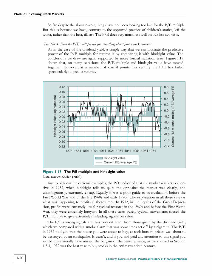
Module 1 / Valuing Stock Markets
1/50 Edinburgh Business School Practical History of Financial Markets
So far, despite the above caveat, things have not been looking too bad for the P/E multiple. But this is because we have, contrary to the approved practice of children's stories, left the worst, rather than the best, till last. The P/E does very much less well on our last two tests.
Test No. 4. Does the P/E multiple tell you something about future stock returns? As in the case of the dividend yield, a simple way that we can illustrate the predictive
power of the P/E multiple for returns is by comparing it with hindsight value. The conclusions we draw are again supported by more formal statistical tests. Figure 1.17 shows that, on many occasions, the P/E multiple and hindsight value have moved together. However, at a number of crucial points this century the P/E has failed spectacularly to predict returns.
Figure 1.17 The P/E multiple and hindsight value
Data source: Shiller (2000)
Just to pick out the extreme examples, the P/E indicated that the market was very expen-sive in 1932, when hindsight tells us quite the opposite: the market was clearly, and unambiguously, extremely cheap. Equally it was a poor guide to overvaluation before the First World War and in the late 1960s and early 1970s. The explanation in all these cases is what was happening to profits at these times. In 1932, in the depths of the Great Depres-sion, profits were extremely low for cyclical reasons; in the 1960s and before the First World War, they were extremely buoyant. In all these cases purely cyclical movements caused the P/E multiple to give extremely misleading signals on value.
The P/E's wrong signals are thus very different from those given by the dividend yield, which we compared with a smoke alarm that was sometimes set off by a cigarette. The P/E in 1932 told you that the house you were about to buy, at rock bottom prices, was about to be destroyed by an earthquake. It wasn't, and if you had paid any attention to this signal you would quite literally have missed the bargain of the century, since, as we showed in Section 1.5.3, 1932 was the best year to buy stocks in the entire twentieth century.
1871 1881 1891 1901 1911 1921 1931 1941 1951 1961 1971
0.12
0.10
0.08
0.06
0.04
0.02
0.00
-0.02
-0.04
-0.06
-0.08
-0.10
-0.12
0.8
0.6
0.4
0.2
0.0
-0.2
-0.4
-0.6
-0.8
-1.0
-1.2
Hindsight value
Current PE/average PE

Module 1 / Valuing Stock Markets
Practical History of Financial Markets Edinburgh Business School 1/51
Why does the P/E provide such unreliable signals? The explanation can be found by looking at our fifth and final test.
Test No. 5. Does the P/E multiple have a stable ‘fundamental’? No. Corporate earnings, which, as Box 3 explains, represent the ‘fundamental’ for the
price-earnings multiple, are highly volatile. As a result, the P/E multiple clearly does not so obviously have the convenient property we noted when we set up this fourth test, that an indicator of over- or undervaluation should mainly rise or fall when the stock price rises or falls.
The primary, but by no means the only, reason for this volatility is that profits are highly dependent on the state of the economy. When the economy goes into recession, employment and wages both weaken but sales usually fall much more quickly. This squeezes operating margins. Meanwhile the charges for depreciation and interest continue. What is left over, which is firm's profits, can thus fall like the proverbial stone.
1932 provides the most extreme example this century, and explains why the alarm signal given by the P/E was so radically misleading. National accounts statistics for that year show that the corporate sector as a whole was actually making losses.29 If quoted companies’ profits had moved in line, therefore, the P/E multiple should actually have gone negative! In fact, whether by dint of creative accounting, or by superior performance, quoted companies managed in aggregate to show some profits. But, since earnings per share fell by more than the stock price (which was itself at this point falling even faster than the proverbial stone), the P/E multiple rose, rather than fell, as the stock market, in reality, got progressively cheaper.
The P/E was giving the wrong signal because current earnings in 1932 gave a highly mis-leading indication of the potential profitability of the US corporate sector. 1932 was by far the most extreme case, but Figure 1.17 showed that it was by no means the only occasion when the P/E gave misleading signals. In the next chapter we shall look at ways to deal with the problems presented by the volatility of profits. Unfortunately the problem cannot be solved in a fully satisfactory way. However, we shall see that, if it could, the result would lead to the same answer as our favoured valuation indicator, q.
The other problem with the P/E multiple is that it sometimes works the wrong way round, like a smoke alarm that goes off too late. Knowing that your alarm will go off after your house has burnt down is among the most useless pieces of information that it is possible to imagine.
But this order of events should really cause no surprise. It is often claimed that the stock market is a leading indicator, rising before the economy recovers from a recession and peaking before the boom ends. Such claims about the stock market's predictive power are at least sometimes correct – hence the old joke that that the stock market has predicted twelve of the past nine recessions.
Since the stock market is sometimes correct in predicting the state of the economy, it will also predict earnings, because, as we have already noted, earnings tend to rise and fall with the economy. So a high or low P/E may simply indicate that the stock market is predicting a cyclical recovery, or a cyclical collapse in earnings. This clouds the picture and severely devalues the ability the of P/E multiple to indicate value.
29 See Wright (op cit).

Module 1 / Valuing Stock Markets
1/52 Edinburgh Business School Practical History of Financial Markets
1.10.2 Conclusions: The P/E Multiple as an Indicator of Stock Market Value
Table 1.3 summarises the performance of the P/E multiple (and hence of course of the earnings yield) in relation to our five tests.
Table 1.3 The P/E multiple and the five key tests for any indicator of value 1. Measurable? Yes, but profits figures may be suspect, and so‘fair’ value
for P/E is in doubt.
2. Mean reversion? Yes.
3. Makes economic sense? Only if ‘Siegel's Constant’ actually is constant.
4. Weakly predicts stock returns? No. Its signals are inaccurate, and sometimes perverse.
5. Stable fundamental? No.
The table makes it clear that, while the P/E multiple remedies some of the faults of the dividend yield, it does so only by introducing other problems. In the next section, we shall examine two alternative ways in which attempts are often made to rectify these problems.
1.11 The Adjusted Price-Earnings Multiple The P/E multiple is so widely used for assessing value that ways around the problems we identified in the last chapter have naturally been sought. There have been two main approaches. The first has been to try to forecast future earnings, and the second has been to try to adjust earnings to allow for the cyclical swings in the economy.
1.11.1 The Prospective P/E Multiple
The first approach, which results in an adjusted P/E multiple normally referred to as the prospective P/E, is widely used by stockbrokers, and there is no doubt that it is admirably suited to its purpose, which is to sell shares. As the profit forecasts are purely subjective, so are the prospective P/Es that result. It is thus without merit or utility for the purpose of seeking an objective criterion of value. We shall therefore not give it the full treatment that we have awarded to other competing indicators of value.
We only pause briefly to note the obvious reason why stockbrokers tend to prefer the prospective P/E to the usual measure (often, in such comparisons, referred to as the ‘historic’ P/E – a term generally used in a somewhat disparaging manner, as if being true were a severe disadvantage). This is that it almost invariably turns out lower, and hence can be interpreted, if you do not look too hard, as indicating better value. But there are two fairly obvious explanations of why the apparent impression of better value is entirely spurious.
The first is the natural tendency for stockbrokers' forecasts to see the future through rose-tinted spectacles. This is illustrated in Figure 1.18, which is taken from a recent study by Professor Sushil Wadhwani. The chart shows that even during the boom years of the 1990s, when profits did not suffer any significant setbacks, brokers’ forecasts were on average 7% higher than the actual outturn, and sometimes very much more so. A persistent upward bias in forecasts of earnings per share must imply a persistent downward bias in the prospective P/E multiple.30
30 The figures for the chart are from Figure 4 in Sushil Wadhwani, ‘The US stock market and the global economic crisis’, National Institute Economic Review, January 1999, pp.86–109. The chart shows the difference between IDES 12 month ahead earnings forecasts and actual outturns.

Module 1 / Valuing Stock Markets
Practical History of Financial Markets Edinburgh Business School 1/53
Figure 1.18 The upward bias in stockbrokers' earning forecasts
There is a second (albeit normally less important) reason why prospective P/Es are lower than historic P/Es. This would be the case even if (a big ‘if’) stockbrokers’ forecasts were usually on target. A moment's thought reveals why. If, as has been the case for the past 50 years or so, earnings per share tend to grow over time, through a combination of modest real growth, and sometimes rather less modest inflation, then next year's earnings will on average always be higher than this year's, so that the prospective P/E would be below the historic P/E even with unbiased forecasts of earnings.
If we take both of these factors into account, it is quite easy to pull down the prospective P/E by quite a significant amount compared with the historic P/E, and stockbrokers are particular prone to exploit this at times when the historic P/E points to overvaluation. Over the past 50 years, both real growth of earnings per share and inflation have averaged around 4%, giving an average annual growth of earnings per share in dollar terms of around 8%. If on top of that we build in, say, a 15% bias in brokers’ forecasts (allowing for the fact that these forecasts tend to be most bullish – when they need to be bullish, that is, when earnings are low, or the P/E is high), then forecast earnings will be of the order of 25% higher than historic earnings, and the prospective P/E will be brought down accordingly.
At the peak of the boom, this did not do enough to help even the prospective P/E mul-tiple to provide a sufficiently rosy picture, so it tended to fall out of favour with stockbrokers. However, after the falls in the US market, when the remaining degree of overvaluation was much more modest, a careful use of the prospective P/E multiple could quite easily appear to eliminate the overvaluation entirely, so it has begun to regain populari-ty in its key role, as a means of persuading people to buy shares. As an indicator of value, however, it remains as useless as ever.
1.11.2 The Cyclically Adjusted Price-Earnings Multiple
The second approach involves adjusting the P/E multiple to allow for the cyclical fluctua-tions in profits that we discussed in the previous chapter. This is of much greater potential interest, and so we consider it more thoroughly.
–40
–30
–20
–10
0
10
20
30
40
50
8.1.86 12.1.88 15.1.90 17.1.92 19.1.94 24.1.96
Module 1 / Valuing Stock Markets
1/54 Edinburgh Business School Practical History of Financial Markets
If it were possible to adjust current earnings so as to remove the element of cyclical fluctuation and reveal, as it were, their true underlying level, then we shall see that the P/E multiple derived from these adjusted earnings might provide a valid measure of the stock market's value. In order to show why, we shall initially simply assume that such an adjust-ment could be made. This has the advantage of allowing us to ignore for the time being the various different ways in which it might be possible to do so. We shall therefore apply our five usual tests to the cyclically adjusted P/E, but, in this section, in order to simplify the argument, we shall not carry them out in the usual order, leaving the first test, of measurabil-ity, until last.
Test No. 2. Does the cyclically adjusted P/E multiple mean-revert? It may seem strange to answer this question when we have not dealt with the issue of
how cyclical adjustment is to be carried out, but in fact we can answer it by a simple application of logic. If the unadjusted P/E mean-reverts, then the cyclically adjusted P/E must mean-revert as well. Since we have seen that there is strong historical evidence for the former, the latter follows automatically.
The reason for this is straightforward. If we think about the concept of cyclical adjust-ment, it should be fairly evident that any such adjustment, however carried out, must cancel out over the course of a full economic cycle. Thus, if earnings are depressed in a recession, the cyclical adjustment will raise adjusted earnings; but if they are boosted in a boom, the cyclical adjustment will lower them. Over a complete economic cycle the adjustments should net out, so that the average of actual earnings over the cycle should equal the average of adjusted earnings. Only the path through the cycle should differ.
A useful analogy can be drawn with the process of seasonal adjustment carried out on most economic data by national accountants. Actual (unadjusted) GDP is, for example, always weak in the winter months, because seasonal activities such as construction and agriculture fall back to low levels. Data for seasonally adjusted GDP thus give a more accurate picture of the underlying movements in national output. But annual figures for seasonally adjusted and unadjusted GDP must be, and are identical; only the quarterly paths differ.
The analogy with seasonal adjustment also points, of course, to a significant difference. Everyone knows how long a year is, but identifying the length of a particular economic cycle is far, far harder. However, despite the practical difficulties, to which we shall return, the fundamental principle that cyclical adjustments should cancel out is inescapable.31
Anything that cancels out over time must by definition be mean-reverting, with a mean of zero, or one, depending on whether adjustments are in dollar terms, or in proportional terms. The difference between the actual P/E multiple and any cyclically adjusted P/E multiple must therefore be mean-reverting. If you add or multiply two mean-reverting series, the result is still mean-reverting. So if the unadjusted P/E mean-reverts, the cyclically adjusted P/E must too.
31 This has not, of course, prevented many attempts to escape it. Stockbrokers frequently adjust earnings upwards in a
recession on cyclical grounds, but then (we assume out of absent-mindedness) forget to introduce an offsetting downward adjustment in the boom. Finance ministries tend to do exactly the same to GDP and tax receipts.

Module 1 / Valuing Stock Markets
Practical History of Financial Markets Edinburgh Business School 1/55
Test No 3. Does the cyclically adjusted P/E multiple make economic sense as an indicator of value? Since cyclical adjustments must cancel out over long enough periods, and the economic
rationale for value can only hold in long-run terms, in general the strengths and weaknesses of the economic case for the cyclically adjusted P/E are the same as those for the unadjusted P/E. However, we shall see in due course that, if the cyclical adjustment were done in an ‘ideal’ way, the cyclically adjusted P/E would produce exactly the same indication of value as q.
We deal with the next two tests together.
Test No. 4. Does the cyclically adjusted P/E multiple tell you anything about future stock returns? and Test no 5. Is the ‘fundamental’ for the cyclically adjusted P/E multiple stable? Again, we can answer both questions by the application of logic. If the cyclical adjust-
ment could be done properly, the cyclically adjusted P/E must tell you something about future stock returns. Once the adjustment had been made, the earnings for each year would move rather slowly, and would normally be a bit higher, measured in real terms, than those for the year before. This immediately overcomes one of the difficulties we identified in the last chapter when looking at actual P/E multiples, which is that earnings fluctuate too much. Since, as we have already seen, the cyclically adjusted P/E must also mean-revert, and cyclically adjusted earnings must be smooth, this would necessarily imply that the mean reversion would come about through changes in the stock price, and hence through returns.
Notice, however, our use of the conditional. For, while we regard the cyclically adjusted P/E as a very useful concept, we have left until last the test that identifies its primary weakness in practical terms. This is the problem of measurability.
Test No. 1. Does the cyclically adjusted P/E multiple provide a measurable indicator of value? We now need to address the question, that we side-stepped earlier, of how cyclical
adjustment should actually be carried out. We have been assuming up until now that, however it was actually done, it was done in a way that clearly met our key conditions, that cyclical adjustment should remove the volatility in earnings due to recessions and booms, and, crucially, that it should do so in a way that cancels out over a full cycle. The problem is that, to do this job properly, you need to be able to see into the future.
We said when we looked at the last two tests that it would be expected that cyclically adjusted profits should have a tendency to rise gradually over time. But this begs the question of why, and by how much. We shall postpone for now a full discussion of ‘why’, until we deal with this issue properly by showing the link with q. But we can see even on a cursory examination that the question of ‘how much’ can only be answered properly if we can see into the future.
In the simplest terms, if profits are being driven by the state of the economy, we need to know two things: first, where the economy is in relation to its long-run potential; and second, how much profits are being affected by this. When we look back at past booms and recessions, we can at least make a reasonable attempt to answer both these questions, with the benefit of hindsight. We can, for example, usually identify turningpoints in output after the event, and there are methods that can be applied to identify the average amount by which, for example,
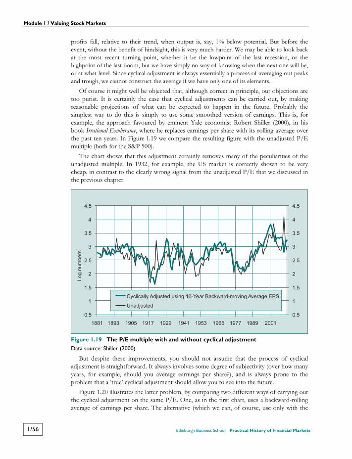
Module 1 / Valuing Stock Markets
1/56 Edinburgh Business School Practical History of Financial Markets
profits fall, relative to their trend, when output is, say, 1% below potential. But before the event, without the benefit of hindsight, this is very much harder. We may be able to look back at the most recent turning point, whether it be the lowpoint of the last recession, or the highpoint of the last boom, but we have simply no way of knowing when the next one will be, or at what level. Since cyclical adjustment is always essentially a process of averaging out peaks and trough, we cannot construct the average if we have only one of its elements.
Of course it might well be objected that, although correct in principle, our objections are too purist. It is certainly the case that cyclical adjustments can be carried out, by making reasonable projections of what can be expected to happen in the future. Probably the simplest way to do this is simply to use some smoothed version of earnings. This is, for example, the approach favoured by eminent Yale economist Robert Shiller (2000), in his book Irrational Exuberance, where he replaces earnings per share with its rolling average over the past ten years. In Figure 1.19 we compare the resulting figure with the unadjusted P/E multiple (both for the S&P 500).
The chart shows that this adjustment certainly removes many of the peculiarities of the unadjusted multiple. In 1932, for example, the US market is correctly shown to be very cheap, in contrast to the clearly wrong signal from the unadjusted P/E that we discussed in the previous chapter.
Figure 1.19 The P/E multiple with and without cyclical adjustment
Data source: Shiller (2000)
But despite these improvements, you should not assume that the process of cyclical adjustment is straightforward. It always involves some degree of subjectivity (over how many years, for example, should you average earnings per share?), and is always prone to the problem that a ‘true’ cyclical adjustment should allow you to see into the future.
Figure 1.20 illustrates the latter problem, by comparing two different ways of carrying out the cyclical adjustment on the same P/E. One, as in the first chart, uses a backward-rolling average of earnings per share. The alternative (which we can, of course, use only with the
0.5
1
1.5
2
2.5
3
3.5
4
4.5
0.5
1
1.5
2
2.5
3
3.5
4
4.5
1881 1893 1905 1917 1929 1941 1953 1965 1977 1989 2001
Log n
um
bers
Cyclically Adjusted using 10-Year Backward-moving Average EPS
Unadjusted
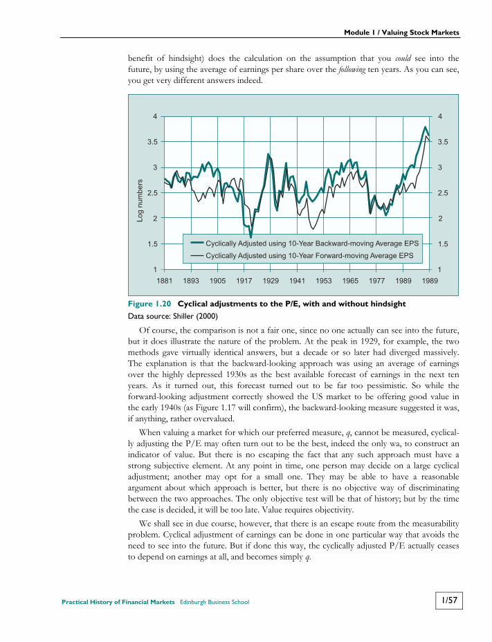
Module 1 / Valuing Stock Markets
Practical History of Financial Markets Edinburgh Business School 1/57
benefit of hindsight) does the calculation on the assumption that you could see into the future, by using the average of earnings per share over the following ten years. As you can see, you get very different answers indeed.
Figure 1.20 Cyclical adjustments to the P/E, with and without hindsight
Data source: Shiller (2000)
Of course, the comparison is not a fair one, since no one actually can see into the future, but it does illustrate the nature of the problem. At the peak in 1929, for example, the two methods gave virtually identical answers, but a decade or so later had diverged massively. The explanation is that the backward-looking approach was using an average of earnings over the highly depressed 1930s as the best available forecast of earnings in the next ten years. As it turned out, this forecast turned out to be far too pessimistic. So while the forward-looking adjustment correctly showed the US market to be offering good value in the early 1940s (as Figure 1.17 will confirm), the backward-looking measure suggested it was, if anything, rather overvalued.
When valuing a market for which our preferred measure, q, cannot be measured, cyclical-ly adjusting the P/E may often turn out to be the best, indeed the only wa, to construct an indicator of value. But there is no escaping the fact that any such approach must have a strong subjective element. At any point in time, one person may decide on a large cyclical adjustment; another may opt for a small one. They may be able to have a reasonable argument about which approach is better, but there is no objective way of discriminating between the two approaches. The only objective test will be that of history; but by the time the case is decided, it will be too late. Value requires objectivity.
We shall see in due course, however, that there is an escape route from the measurability problem. Cyclical adjustment of earnings can be done in one particular way that avoids the need to see into the future. But if done this way, the cyclically adjusted P/E actually ceases to depend on earnings at all, and becomes simply q.
1
1.5
2
2.5
3
3.5
4
1
1.5
2
2.5
3
3.5
4
1881 1893 1905 1917 1929 1941 1953 1965 1977 1989 1989
Log n
um
bers
Cyclically Adjusted using 10-Year Backward-moving Average EPS
Cyclically Adjusted using 10-Year Forward-moving Average EPS
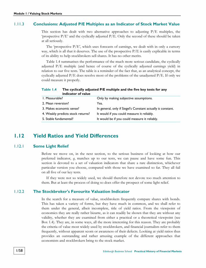
Module 1 / Valuing Stock Markets
1/58 Edinburgh Business School Practical History of Financial Markets
1.11.3 Conclusions: Adjusted P/E Multiples as an Indicator of Stock Market Value
This section has dealt with two alternative approaches to adjusting P/E multiples, the ‘prospective P/E’ and the cyclically adjusted P/E. Only the second of these should be taken at all seriously.
The ‘prospective P/E’, which uses forecasts of earnings, we dealt with in only a cursory way, which is all that it deserves. The use of the prospective P/E is easily explicable in terms of its ability to help stockbrokers sell shares. It has no other merits.
Table 1.4 summarises the performance of the much more serious candidate, the cyclically adjusted P/E multiple (and hence of course of the cyclically adjusted earnings yield) in relation to our five tests. The table is a reminder of the fact that, as an analytical concept, the cyclically adjusted P/E does resolve most of the problems of the unadjusted P/E. If only we could measure it properly.
Table 1.4 The cyclically adjusted P/E multiple and the five key tests for any indicator of value
1. Measurable? Only by making subjective assumptions.
2. Mean reversion? Yes.
3. Makes economic sense? In general, only if Siegel's Constant actually is constant.
4. Weakly predicts stock returns? It would if you could measure it reliably.
5. Stable fundamental? It would be if you could measure it reliably.
1.12 Yield Ratios and Yield Differences
1.12.1 Some Light Relief
Before we move on, in the next section, to the serious business of looking at how our preferred indicator, q, matches up to our tests, we can pause and have some fun. This section is devoted to a set of valuation indicators that share a rare distinction, whichever particular version you choose, compared with those we have examined so far. They all fail on all five of our key tests.
If they were not so widely used, we should therefore not devote too much attention to them. But at least the process of doing so does offer the prospect of some light relief.
1.12.2 The Stockbroker's Favourite Valuation Indicator
In the search for a measure of value, stockbrokers frequently compare shares with bonds. This has taken a variety of forms, but they have much in common, and we shall refer to them under the general, albeit incomplete, title of yield ratios. From the viewpoint of economics they are really rather bizarre, as it can readily be shown that they are without any validity, whether they are examined from either a practical or a theoretical viewpoint (see Box 1.4). They are, in some ways, all the more interesting for this reason. They are probably the criteria of value most widely used by stockbrokers, and financial journalists refer to them frequently, without apparent scorn or awareness of their defects. Looking at yield ratios thus provides an outstanding and rather amusing example of the different approaches that economists and stockbrokers bring to the stock market.

Module 1 / Valuing Stock Markets
Practical History of Financial Markets Edinburgh Business School 1/59
As far as we can tell, the first ratio of this type that was claimed as useful for valuing shares was the ratio between bond yields and dividend yields. For example, the yield on long-dated Treasury bonds was compared with the average dividend yield on the S&P Composite Index, and if the ratio was less than, say, 2, shares were declared to be cheap. During the late 1990s, however, even this ratio tended to show that the stock market was expensive, and there was therefore a tendency to change to the ratio between bond yields and earnings or to the difference in yields rather than to the ratio. As these indicators, in turn, showed stocks to be expensive, the fashion changed once again.
A particular charm of yield ratios from the viewpoint of stockbrokers lies in the fact that profits and interest rates tend to move in the same direction. In a strong economy, profits are strong and interest rates rise. In a weak economy the opposite happens. Stockbrokers using yield ratios should therefore never be without some good news that they can use for selling stocks.
Box 1.4: (Mis-)Using the Dividend Discount Model to Rationalise Yield Gaps __________________________________ If we write down the Dividend Discount Model yet again, as
we can, if we ignore the necessary mutual dependence of the elements in the model, provide an apparent (but actually entirely illusory) rationale for looking at yield gaps or yield ratios.
First, we need to assume that the typical investor's desired return on bonds, or some other competing asset, is given by actual bond yields, B. This is by no means an innocuous assumption.
Second, we need to assume that the typical investor demands a constant premium, ρ, from equities, compared with the expected return on bonds, i.e.
Third, we assume (in a way that is clearly contrary to the logic of Box 3) that we can simply take G as given.
Using all these assumptions, we can rewrite the Dividend Discount Model as
or, rearranging,
If we are prepared to assume that the right-hand side of this expression is constant, then this might appear to suggest that we can use the difference between the bond yield and the dividend yield as an indicator of value: hence when bond yields are high in relation to the dividend yield, it would imply that the market was overvalued, and vice versa.
In fact, this implies major errors in logic.
First, in order to do this, of course, we have to ignore all the problems associated with instability of the dividend yield that we discussed in Boxes 1.2 and 1.3, which imply that G cannot simply be taken as given.
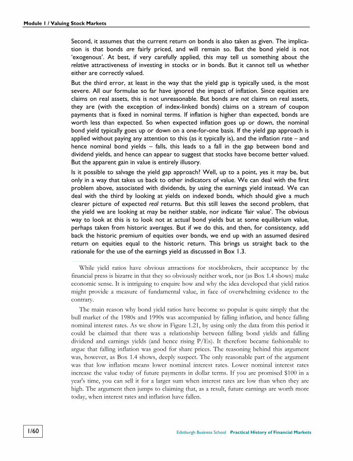
Module 1 / Valuing Stock Markets
1/60 Edinburgh Business School Practical History of Financial Markets
Second, it assumes that the current return on bonds is also taken as given. The implica-tion is that bonds are fairly priced, and will remain so. But the bond yield is not ‘exogenous’. At best, if very carefully applied, this may tell us something about the relative attractiveness of investing in stocks or in bonds. But it cannot tell us whether either are correctly valued.
But the third error, at least in the way that the yield gap is typically used, is the most severe. All our formulae so far have ignored the impact of inflation. Since equities are claims on real assets, this is not unreasonable. But bonds are not claims on real assets, they are (with the exception of index-linked bonds) claims on a stream of coupon payments that is fixed in nominal terms. If inflation is higher than expected, bonds are worth less than expected. So when expected inflation goes up or down, the nominal bond yield typically goes up or down on a one-for-one basis. If the yield gap approach is applied without paying any attention to this (as it typically is), and the inflation rate – and hence nominal bond yields – falls, this leads to a fall in the gap between bond and dividend yields, and hence can appear to suggest that stocks have become better valued. But the apparent gain in value is entirely illusory.
Is it possible to salvage the yield gap approach? Well, up to a point, yes it may be, but only in a way that takes us back to other indicators of value. We can deal with the first problem above, associated with dividends, by using the earnings yield instead. We can deal with the third by looking at yields on indexed bonds, which should give a much clearer picture of expected real returns. But this still leaves the second problem, that the yield we are looking at may be neither stable, nor indicate ‘fair value’. The obvious way to look at this is to look not at actual bond yields but at some equilibrium value, perhaps taken from historic averages. But if we do this, and then, for consistency, add back the historic premium of equities over bonds, we end up with an assumed desired return on equities equal to the historic return. This brings us straight back to the rationale for the use of the earnings yield as discussed in Box 1.3. __________________________________________________________________________________________________________________________________________________________________________________________________________________________________________________________________________________________________________________________________________________________________________________________________________________________________________________________________________________________________________________________________________________________________________________________________________________________________________________________________________________________
While yield ratios have obvious attractions for stockbrokers, their acceptance by the financial press is bizarre in that they so obviously neither work, nor (as Box 1.4 shows) make economic sense. It is intriguing to enquire how and why the idea developed that yield ratios might provide a measure of fundamental value, in face of overwhelming evidence to the contrary.
The main reason why bond yield ratios have become so popular is quite simply that the bull market of the 1980s and 1990s was accompanied by falling inflation, and hence falling nominal interest rates. As we show in Figure 1.21, by using only the data from this period it could be claimed that there was a relationship between falling bond yields and falling dividend and earnings yields (and hence rising P/Es). It therefore became fashionable to argue that falling inflation was good for share prices. The reasoning behind this argument was, however, as Box 1.4 shows, deeply suspect. The only reasonable part of the argument was that low inflation means lower nominal interest rates. Lower nominal interest rates increase the value today of future payments in dollar terms. If you are promised $100 in a year's time, you can sell it for a larger sum when interest rates are low than when they are high. The argument then jumps to claiming that, as a result, future earnings are worth more today, when interest rates and inflation have fallen.

Module 1 / Valuing Stock Markets
Practical History of Financial Markets Edinburgh Business School 1/61
Figure 1.21 Do bond and equity yields move in the same direction? (1981–98)
The supreme nonsense of this argument is best illustrated by comparing it with the exact opposite view, which was held, generally with equal enthusiasm, in the previous 20-year bull market, from 1948 to 1968, and which we illustrate in Figure 1.22. In this period inflation was rising, and there was an equally accidental correlation between rising bond yields and rising P/Es. It is interesting to note that, from a statistical viewpoint, the evidence in this earlier period, which exactly contradicts the bond yield ratio, was actually stronger than it was in support of the theory in the later period. While the stock market, interest rates and inflation were all rising together in the 1950s and 1960s, it was then believed that inflation was good for shares. The theory used to support the argument was that inflation would boost future earnings, and that shares were worth more today because earnings in the future would be higher.
In practice, of course, neither of these mutually contradictory theories holds up. Inflation increases both future profits and interest rates, in nominal terms. The result is that the two factors knock each other out, and it makes no difference whatever to the fundamental value of stocks if the rate of inflation rises or falls.
0
4
8
12
16
20
24
1981 1983 1985 1987 1989 1991 1993 1995 1997
0
2
4
6
8
10
12Bond yield (left scale)Dividend yield (right scale)Earnings yield (right scale)
y

Module 1 / Valuing Stock Markets
1/62 Edinburgh Business School Practical History of Financial Markets
Figure 1.22 …Or do bond and equity yields move in opposite directions? (1950–68)
The statistical case for valuing equities in relation to either bond yields or inflation is a prime example of selecting data to support the case you wish to make, rather than using it objectively in an attempt to discover the truth. In other words, it is data mining, against which we issued a warning in Section 1.7. Figure 1.21 shows that when all the available information is used there is essentially no correlation between bond yields and dividend yields or P/E multiples. Theoretical expectations are thus borne out in practice.
This illustrates nicely the difference between real economics and stockbroker economics. Economists, when faced with a conflict between theory and evidence, discard their theory. Stockbrokers discard the evidence. Bond yield ratios are a prime illustration of this.
For the sake of completeness, we now briefly examine yield ratios in relation to our four key tests.
Test No. 1. Do yield ratios and related indicators provide a measurable indicator of value? No. It is true that the only new element that enters when we consider yield ratios and
related indicators is the long-term interest rate, which can be measured with some precision. However, as we discovered in the case of the dividend yield, simply having something that is well measured does not of itself imply that the associated indication of value can be so well measured, or indeed measured at all. We noted at the start of this chapter that at one time it was felt that the appropriate ratio between the bond yield and the dividend yield was two. This particular number, we also noted, has now fallen out of favour. As well it may, for there is neither a statistical nor an economic case for any particular number. Without that crucial number, however, it is impossible even to begin to use yield ratios to give an indication of value.
0
1
2
3
4
5
6
7
8
9
1950 1952 1954 1956 1958 1960 1962 1964 1966 1968
0
2
4
6
8
10
12
14
16
18
Bond yield (left scale)
Dividend yield (right scale)Earnings yield (right scale)

Module 1 / Valuing Stock Markets
Practical History of Financial Markets Edinburgh Business School 1/63
Test No. 2. Do yield ratios and related indicators mean-revert? No. One of the most obvious features of the history of yield ratios is that they clearly
do not mean-revert. There is no ambiguity about this. Nor should this be at all surpris-ing. Figure 1.23 summarises the evidence by looking at the most common definition, the ratio of the bond yield to the dividend yield. A similar picture would emerge for all alternative measures of this type.
Figure 1.23 The yield ratio*, 1871–2010
*Ratio of long-term government bond yield to dividend yield. Data source: Shiller (2000)
Table 1.5 helps to explain why. It compares average bond yields, dividend yields and earnings yields over a range of different periods. We have already pointed out that earnings yields have been mean-reverting, and that even dividend yields have shown some degree of stability. This indeed has been one of their key attractions for the use of either as potential measures of value. Average bond yields, however, have been far from stable, as they have fluctuated greatly with inflation, being much higher over the past 30 years that, they were over the previous periods. The tendency for stockbrokers to prefer bond yield ratios over dividend or earnings yields has therefore constituted a preference for something that most clearly doesn't work over something that may be imperfect but has a much better claim to be useful, even if subject to the objections we have raised in the preceding chapters.
Table 1.5 shows that the yield ratios that can be derived from these figures are thoroughly unstable. Average ratios were very different in the last 30 years than they were before, and the difference is associated with very different levels of inflation.
Earnings yield/Bond
Dividend yield/Bond
4.5
4.0
3.5
3.0
2.5
2.0
1.5
1.0
0.5
0.0
9.0
8.0
7.0
6.0
5.0
4.0
3.0
2.0
1.0
0.020011991198119711961195119411931192119111901189118811871

Module 1 / Valuing Stock Markets
1/64 Edinburgh Business School Practical History of Financial Markets
Table 1.5 The myth of yield ratios 1871–1997 Correlation and coefficient
Bond and earnings yield 0.08
Bond and dividend yield −0.13
Time period Average Average Average Average
inflation dividend earnings Bond
rate yield yield yield
1871–1997 2.1 4.8 8.1 4.9
1928–1948 3.1 5.2 7.6 1.6
1948–1968 1.7 4.6 8.6 3.2
1968–1997 4.7 3.9 8.2 7.9
Test No. 3. Do yield ratios and related indicators make economic sense as an indicator of value? Again, unambiguously no. It should be said, in defence of some who have used yield
ratios, that it has at least sometimes been based on some idea, albeit mistaken, that the ratio might be theoretically justified. As Box 4 shows, to the extent that it has any economic rationale at all, the use of yield ratios is based on the use, or more appropri-ately misuse, of the Dividend Discount Model. On closer examination, however, the fact that yield ratios provide no guide to stock market value is no surprise whatever, since they have no economic basis. Indeed it would be a grave shock if they did. This is because shares represent the ownership of real assets, whereas bonds only provide an income that is fixed in nominal terms. Shares should therefore provide a protection against inflation, at least in the longer term, that bonds don't provide. Changes in inflation thus cause interest rates to rise and fall, but there is no reason to expect them to affect dividend or earnings yields. The ratio of bond yields to earnings or dividend yields should therefore vary with inflation, being high when inflation is high and vice versa. In fact, theory correctly forecasts what has happened. As Figure 1.23 shows, the ratio between the long-term bond yield and the dividend yield was low when inflation was low, but rose steadily in the more inflationary period after the Second World War.
In recent years a number of governments have begun to issue ‘index-linked bonds’ where both the interest and principle are guaranteed in real rather than nominal terms. Compari-sons between the yields on index-linked bonds and shares do not therefore suffer from being affected by changes in inflation. But, as explained in Box 1.4, this only deals with one of the major errors in logic that underlie the use of yield ratios and yield differences. It also shows that, if you deal with the other problems, you are taken straight back to the use of the P/E multiple.
Test No. 4. Do yield ratios and related indicators tell you anything about future stock returns? No. We can again answer this question using logic alone. We saw previously that mean
reversion of any indicator is a necessary, but not a sufficient, condition to be a useful indicator of stock market value. Yield ratios do not come anywhere near satisfying the necessary condition; therefore they cannot possibly satisfy the sufficient condition.
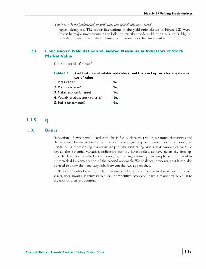
Module 1 / Valuing Stock Markets
Practical History of Financial Markets Edinburgh Business School 1/65
Test No. 5. Is the fundamental for yield ratios and related indicators stable? Again, clearly no. The major fluctuations in the yield ratio shown in Figure 1.23 were
driven by major movements in the inflation rate that made yield ratios, as a result, highly volatile for reasons entirely unrelated to movements in the stock market.
1.12.3 Conclusions: Yield Ratios and Related Measures as Indicators of Stock Market Value
Table 1.6 speaks for itself.
Table 1.6 Yield ratios and related indicators, and the five key tests for any indica-tor of value
1. Measurable? No.
2. Mean reversion? No.
3. Makes economic sense? No.
4. Weakly predicts stock returns? No.
5. Stable fundamental? No.
1.13 q
1.13.1 Basics
In Section 1.3, when we looked at the basis for stock market value, we noted that stocks and shares could be viewed either as financial assets, yielding an uncertain income from divi-dends, or as representing part-ownership of the underlying assets that companies own. So far, all the potential valuation indicators that we have looked at have taken the first ap-proach. The ratio usually known simply by the single letter q may simply be considered as the practical implementation of the second approach. We shall see, however, that it can also be used to show the necessary links between the two approaches.
The simple idea behind q is that, because stocks represent a title to the ownership of real assets, they should, if fairly valued in a competitive economy, have a market value equal to the cost of their production.

Module 1 / Valuing Stock Markets
1/66 Edinburgh Business School Practical History of Financial Markets
q is the ratio of the market value of companies to the replacement cost of their assets. It may be expressed in either of two forms:
either Marketvalueofequities
Tangibleassets NetcorporatedebtEquity
or Marketvalueofequities Netcorporatedebt
TangibleassetsTobin′s
Both definitions have some conceptual advantages. The second definition, Tobin's q, is named after Nobel Laureate James Tobin. It has historical priority, since Tobin's famous paper demonstrating the equilibrium relationship between market value and replacement cost of assets was the first to refer to the ratio as q.32 It also appeals to economists, as the market value of corporate assets should not change when managements decide to finance their companies with more or less equity relative to debt.33
The principles behind q are straightforward. Provided that the replacement cost of com-pany assets and the stock market's valuation of companies can be ascertained, it is obviously a simple matter to measure the ratio between them.
Companies do not normally publish data on the replacement cost of their assets. Their accounts are based on historic cost (and hence are at ‘book value’), and need to be adjusted for the impact of inflation or deflation. But this does not provide major problems, particu-larly when the data are derived from national accounts, taking the corporate sector as a whole, rather than corporate accounts. Indeed, the use of data for the corporate sector in aggregate has distinct advantages, since national accountants are not prone to the same pressures to massage the data as are corporate accountants. On the other hand, they do have to ensure that balance sheet figures for the corporate sector are consistent with other national accounts data, so there is a requirement for mutual consistency, in the national accounts-based data, that is not imposed upon company accounts individually.34
Figure 1.24 provides a comparison of the two measures using US data.
32 ‘A general equilibrium approach to monetary theory’ by James Tobin, Journal of Money, Credit and Banking. 1969, Vol.
1, pp. 15–29. 33 In technical terms, this definition implicitly assumes that the Modigliani–Miller hypothesis of debt–equity neutrality
holds. But the first definition (equity q), which we prefer, has a distinct advantage as a valuation criterion. This is because a given percentage fall in share prices will translate one-for-one into an equal percentage fall in equity q. It will, however, result in a smaller percentage change in the second measure if corporate bond yields, and hence the market value of debt, remain unchanged. Tobin's q will accordingly have a tendency to look like a damped version of equity q.
34 Difficulties with using equity q can arise, however, where companies have large cross-holdings, which is the situation in Japan. During the bubble that took place there in the late 1980s q was misused by including in the value of corporate assets the current market value of the shareholdings in other companies, rather than the replacement cost of the underlying assets. On this absurd basis, the replacement cost of corporate assets rose as share prices rose and, given the high leverage of Japanese companies, the replacement cost, thus defined, actually rose faster. The stockbrokers were then able to make the absurd claim that the higher the stock market went the better value it offered.

Module 1 / Valuing Stock Markets
Practical History of Financial Markets Edinburgh Business School 1/67
Figure 1.24 Measures of q for the non-financial corporate sector
Data sources: Wright and Federal Reserve Z1 Table B.102
We now subject q to our five tests.
Test No. 1. Does q provide a measurable indicator of value? The Federal Reserve has been publishing data on q for the US stock market since 1945
in their Flow of Funds of the United States (‘Z1’) publication. Although either version can be calculated from the data they publish, it is presented with the emphasis on the compari-son at the equity level.
Data on US q are available over the past century. They are published by the Federal Reserve for the period since 1945, and earlier data can be constructed from a number of sources. See Wright (op cit).
As noted above, the data for corporate net worth that are used to generate data for q are not perfect. There are a range of criticisms of q based on data problems. While these criticisms need to be addressed, our overall conclusion is that measurement problems relating to q for the US market are not sufficient to cast doubt on q's leading role as a valuation criterion for this all-important market.35
We shall focus here on one particular issue relating to the measurement of q. In Box 1.5 we show that, in theory at least, we would expect both measures of q to have an average value equal to 1. In a world of imperfect statistics, q, as measured, does not have an average of 1, but of around 0.65. This may seem like quite a large discrepancy; but for a number of reasons it is by no means as worrying as might appear.
35 For a discussion of the major arguments on measurement problems with q, see Andrew Smithers and Stephen
Wright's article in World Economics, cited above. For other markets, data problems are either much more significant, or, in many cases, unfortunately, the required data do not exist. However, we would argue that the insights that q can provide, in terms of economic logic, are also helpful when looking at other valuation indicators, even when data for q itself are not available.
1900 1910 1920 1930 1940 1950 1960 1970 1980 1990 2000
Ra
tio
s a
s d
efin
ed
1.8
1.6
1.4
1.2
1.0
0.8
0.6
0.4
0.2
0
1.8
1.6
1.4
1.2
1.0
0.8
0.6
0.4
0.2
0
Tobin's q
Equity q
Module 1 / Valuing Stock Markets
1/68 Edinburgh Business School Practical History of Financial Markets
The first reason is that if you have ever worked with economic statistics, you will know that it is actually pretty close. It is not 0.03, or 42.6. A useful comparison may be made with other economic statistics. For example, statisticians can measure the trade deficit – the gap between imports and exports – in two different ways, the details of which we need not worry about here. The crucial point is that they routinely produce ‘statistical discrepancies’ between the different measures, which can on occasion easily be as large as the measured deficit itself. It is important to be aware, however, that this occurs despite the fact that the statisticians know that there can be only one true measure of the trade deficit. For this reason, if they see one measure higher than the other, they usually spend a lot of effort attempting to ‘reconcile’ them, yet nonetheless end up with discrepancies. The process of reconciliation, of course, typically involves looking for reasons why the ‘too high’ measure should be reduced, and why the ‘too low’ measure should be increased. This is of course data mining, but at least with good intentions, since the hypothesis that there is only one true measure of the trade deficit must be correct.
If the statisticians who produced one measure of the trade deficit were kept permanently away from the statisticians who produced the alternative measure, and were unaware of their figures, you may be sure that the discrepancies would be very much bigger. But this is in essence the way that figures for q are produced. The top element of q, the market value of non-financial equities, is produced by statisticians in the Federal Reserve Board. By far the most important element that feeds into the figures for corporate net worth is an estimate of the physical capital stock of the corporate sector. These figures are produced by the US Bureau of Economic Analysis, who worry about them in complete isolation. They certainly do not attempt to match the Fed's figures on average, over long periods, which is all that would be expected. In many ways, of course, this very independence is a tremendous advantage, since it means that there is absolutely no incentive for the statisticians to engage in any form of data mining. But it should therefore be no surprise that the numbers are somewhat inconsistent.
The second reason not to be too concerned by the fact that the average value of q, as measured, is less than 1, is that it is very easy to see why a particular form of mismeasure-ment might lead to this result. Fortunately, this does not do much to affect q's usefulness as a valuation criterion.
Of the two elements in the ratio, the top, the market value of equities, is reasonably wellmeasured. The primary problem must therefore lie with the bottom of the ratio. If the ratio itself is on average lower than we would expect, this must imply that net worth is being systematically overstated. Probably the most likely explanation for this lies in the calculation of the capital stock. This is not the place to engage in a long discourse on the methodology of producing capital stock data, on which subject there has been much learned debate amongst economists and statisticians. But, in brief, there are two main problems with attempting to measure the capital stock. One is that you cannot ever measure the capital stock directly; you can measure only the change in the capital stock, as investment less estimated depreciation. At some point (preferably as far back as possible), statisticians simply have to guess the level of the capital stock, onto which they then add the estimated changes. The second serious problem is how to measure the rate at which capital depreciates.
The first of these problems can easily lead to the capital stock being systematically mis-measured, since if the statisticians get it wrong initially, this can easily affect values for years, or even decades afterwards. But, we have to admit, this problem could just as easily lead to

Module 1 / Valuing Stock Markets
Practical History of Financial Markets Edinburgh Business School 1/69
under- as to over-measurement, so, while it makes mismeasurement of q more likely in general, it does not suggest any tendency to a downward bias.
The second problem, of depreciation, is however much more likely to lead to downward bias. When statisticians think about depreciation, they are essentially asking how long it takes for a given piece of capital – whether a machine, or a computer, or a building – to become useless. If a given item is expected to last, say, ten years, they then normally depreciate its value by one tenth of its initial value each year. Given their primary purpose in measuring the capital stock, which is to measure the productive capacity of the nation, this is perfectly reasonable. But there is a sounder economic approach. Capital is not normally replaced when it physically wears out, but when it ceases to be profitable to use it any more. True economic depreciation thus occurs more rapidly than that measured by the statisticians. Since the whole idea of q is an economic concept, an ideal measure of q would use economic depreciation. But if capital is being depreciated too slowly, this must imply that the capital stock is being systematically overstated.
The word ‘systematic’ is a very important one. It provides the third and probably most important reason why we are not too worried by the fact that the average value of q is not 1. If you had a wristwatch that was always ten minutes fast, you would have no problem telling the time, once you had figured out the ‘bias’ in the signal it was giving you. The same applies to q. We would be much more worried about mismeasurement if there were not nearly a century's worth of evidence that it appears to be mismeasured on a pretty consistent basis.
The evidence for this is, of course, the performance of q in relation to the second test, with which we shall deal shortly. There is strong evidence that q mean-reverts. This could not have come about if the mismeasurement were not on a reasonably regular basis. The mismeasurement complicates matters somewhat, because we need in effect to form an estimate of the average measurement error, given that ‘true’ q must have an average of 1. But given more than 100 years' worth of data, we can form a pretty good estimate of the extent of the bias.
Since q is systematically under-recorded, overvaluation is not indicated by whether q is greater or less than 1, but by whether it is greater or less than its average value of around 0.65.
The net worth of corporations at replacement cost is the ‘fundamental’ used in the bot-tom of our preferred ‘equity’ q ratio as given above, i.e.:
Corporatenetworth Corporatetangibleassets Netcorporatedebt
This is similar to the concept of ‘book value’, but the assets are valued at their current cost, not their historic cost, and thus allow for the effect of inflation or deflation. If we scale it down by the average value of q, we can derive an estimate of ‘true’ q, since the resulting fundamental will lead to a series that has a mean of 1.
We can re-express q in per share terms by dividing through both top and bottom of the ratio by the number of shares:
EquityStockprice
Networthpershare
Module 1 / Valuing Stock Markets
1/70 Edinburgh Business School Practical History of Financial Markets
Test No. 2. Does q mean-revert? If you look back at Figure 1.24, you will see that it provides strong visual reassurance
that US q, however measured, does indeed mean-revert. Testing for mean reversion can also be carried out by more formal statistical methods. On such tests US data show that there is strong evidence that q is indeed a mean-reverting series.36
Such tests do not, of course, give a completely unambiguous answer. In statistical terms they suggest that the probability that q does not mean-revert is very low, but is not zero. Such is life, when you are dealing with real data, and the degree of uncertainty that we saw in Section 1.7 is a necessary feature of any indicator of value. Indeed, we are not even entirely unhappy with this result. In general, if a statistical test rejects some hypothesis (in this case, the hypothesis that q does not mean-revert) with 100% probability, this is as often as not because the test has been carried out wrongly in some way, or has even been rigged.
We do not, of course, derive our confidence in q from its strong performance on the mean reversion test alone, which is only one, albeit an essential one, of our tests of value. The P/E multiple, for example, as we have seen, passes the mean reversion test easily as well as q, but falls down badly on others. This does not happen in the case of q. Possibly the most important point of all is that q is the only indicator of value that unambiguously passes our next test.
Test No. 3. Does q make economic sense? The rationale for q is derived from very basic economic principles, set out in Box 5. It is
bound to work, provided only that the economy in which the stock market operates is basically competitive and, while competitive conditions may fluctuate over time, there is not a strong trend towards greater or less monopoly power.
In such conditions, the cost of capital must be equal to its return in equilibrium. This will ensure that there can be no disparity between the value of the market, derived from discounting future dividends at the correct rate, and the net worth of the corporate sector, correctly valued at its replacement cost.
It is important to stress not only that q makes economic sense, but that the way in which it makes economic sense differs in a crucial way from all the other indicators we have looked at so far.
We saw, for example, that the whole basis for using the P/E multiple to value markets rests on its mean reversion. The P/E is just the earnings yield turned upside down, and Box 4 showed that the earnings yield in turn must in the long-term be essentially the same as the return on stocks. So when we look at the P/E we are in effect asking whether the stock market is offering a ‘fair’ return, where our criterion of ‘fairness’ is the historic return on stocks. As we have seen, this does appear to have been stable over the past two centuries – indeed this is why we refer to it as ‘Siegel's Constant’. But the P/E only works if Siegel's Constant is constant. Because economists have not yet figured out an explanation of why this should be, it is perfectly possible in principle that it might not be constant. We could, for example, imagine a set of parallel universes, each of which had a different value of Siegel's Constant. Each of these parallel universes would have a different ‘fair’ return, and would therefore have a different P/E multiple in equilibrium. But, in all of these parallel universes, q would work just as well. Furthermore, it would mean-revert to the same value.
36 Detailed analysis of q's mean reversion and other qualities can be found in Donald Robertson and Stephen Wright. ‘What does q predict?’ (www.econ.bbk.ac.uk/faculty/wright)

Module 1 / Valuing Stock Markets
Practical History of Financial Markets Edinburgh Business School 1/71
There is a simple explanation for this constancy of q in equilibrium. Viewed in its most simple form, q is just a way of comparing prices in different markets. When q is high or low, this implies that the price of buying the corporate sector's assets via the stock market is high or low, compared with buying them directly. Fundamentally, therefore, the argument for q is based solely on an assumption that in the end arbitrage must work.
The most frequent objection to the use of q that we have encountered from non-economists is that it does not allow for the value of intangibles, i.e. the goodwill values that individual companies may include in the balance sheets for items such as patents. These are often the result of investment by companies in research, and where such research pays off in terms of a new product or greater efficiency, the company is able to earn a higher return on its physical capital than it would otherwise be able to do.
The standard view among economists is that aggregate profitability cannot be boosted by such expenditure. If it could, companies that seek to maximise their return on capital, would increase research expenditure without limit. Research is thus similar to advertising. Compa-nies will increase their expenditure on either until it is no longer expected to produce any incremental return. The aggregate value of the benefits arising from investment made in research or advertising, or other forms of innovation, cannot be expected to be more than the costs involved.37
When the views of non-economists conflict with the standard view, it seems that their comments are made in ignorance of the accepted view among economists, since we have not encountered any analysis that acknowledges the existence of the mainstream view and then takes issue with it. Among economists, the issue is whether the investment in research should be depreciated at a different rate from the immediate write-off, which is allowed for corporation tax, and is the standard assumption in the national accounts.
There are probably several sources of confusion among non-economists about the value of intangibles, but the central one arises from the difference between their value in individual instances and their aggregate value.
Although intangibles will have no aggregate value, this does not mean that they will not be valuable assets for individual companies. Indeed, intangible values will exist through pure luck, even without any investment being made in them.
Consider, for example, the normal situation in a competitive, but not perfectly competi-tive, economy. Not all companies will achieve an average return on their capital. Some will have over-invested and others will operate in industries where their competitors have under-invested. In the first instance the return on capital will be below average and in the second above. Since neither the over- nor the under-investment will disappear overnight, the above- or below-average profits should be reflected in the companies being worth premia or discounts from their net worth at replacement cost.
In aggregate, the return on capital will be average, with those achieving better returns offsetting the poor ones. There will be a goodwill value in the case of the former, offset by negative goodwill, which may reasonably be termed ‘illwill’. The latter is not recorded in individual company balance sheets, but if it were there should be no aggregate value for intangibles, as the goodwill and illwill would balance out to produce a zero figure for the total.
37 For a full account of this process see Professor William J. Baumol (2002) ‘The free market innovation machine’,
Princeton University Press.

Module 1 / Valuing Stock Markets
1/72 Edinburgh Business School Practical History of Financial Markets
The same situation will occur when companies spend money or research on advertising. In a competitive economy the benefits will equal the amount spent, but some will have above- and others below-average results from their expenditure. Those, for example, who successfully patent new drugs will have a goodwill value in their shares, but this will be offset by the unsuccessful, for whom the unsuccessful expenditure will reduce their profitability to below average.
However, in the same way as past investment in plant has value today, so does past in-vestment in research. This will not, however, pose a problem for q data, even if no aggregate value is ascribed to this past research. As we have seen, the key is not that the stock of capital is correctly valued, but that any bias towards over- or undervaluation is consistent. The mean reversion of q, based on the official data, is itself important evidence that the aggregate value of intangibles does not seem to create bias that is changing over time. In any event the relative size and likely duration of intangible values reinforces this. For example, the expenditure by corporations on research seems to be 20% or less of their expenditure on capital equipment.
Box 1.5: and the Dividend Discount Model ________________________ We saw in Box 1.3 that we can write the Dividend Discount Model in the form
The desired return on stocks must equal the underlying rate of profits, in relation to the share price. We can rewrite this expression as
//
where e/ is the return on net worth per share (sometimes rather confusingly called the return on equity). Hence the underlying rate of profitability, and q, as defined in the main text, is the ratio of the stock price to net worth per share. Equivalently, we can rearrange as
Thus q will be greater or less than 1 if the return on net worth is greater or less than the desired return from investing in stocks.
We saw in relation to all the other indicators of value that we looked at that, in order for any of them to mean-revert, a minimal requirement was that e, the desired return of the typical investor, be reasonably stable. If you look closely at the expression for q above, you will see that this is not the case for q. All that we need is that there be a stable relationship between the two returns.
In a reasonably competitive economy this relationship should be straightforward: the two returns should be equal: is simply the underlying return on capital, and e is the cost of capital. With competition the cost of capital should in equilibrium equal its return.
Thus suppose (as many people argued in the boom) we were to move to a new world in which the typical investor demands a return that is permanently lower than historic average returns. If this were to happen, the arguments of Box 1.3 should have made clear that the earnings yield must also fall on a sustained basis, and hence the equilibrium P/E multiple would have to rise above its historic average. But competition should ensure that q still reverts to its historic average, since if the cost of capital falls, the only
Module 1 / Valuing Stock Markets
Practical History of Financial Markets Edinburgh Business School 1/73
outcome in equilibrium must be that the return on capital also falls, one for one: i.e., firms would simply become less profitable. This framework also allows us to address the only two potential problems with q: mismeasurement, and failures of competition. If there is systematic overstatement of capital, then this would explain why the mean value of measured q is less than 1: overstatement of capital implies understatement of underlying returns. At the height of the boom there were also arguments in the opposite direction: some argued that capital was being increasingly understated, implying that true q was not nearly so high as the data suggested. These claims were, however, fairly implausible even at the height of the boom, and their credibility has not been improved by subsequent events. Amongst other problems with this argument, it required that profits and GDP must have been radically underestimated in the 1990s.38 An alternative rationale for a permanently higher level of q requires the assumption that markets become less competitive on average. If there is an element in profits due to entrenched monopoly power, this may in principle mean that underlying returns (as measured by ) may permanently differ from the cost of capital. But monopoly profits, of course, are nothing new; so if this is to be used as a rationale for permanently higher q it must be assumed not just that there monopoly profits but that these are perma-nently higher than in the past. It is virtually impossible to reconcile the rise in the 1990s with any possible rise in monopoly power, even if there were any evidence for this, which there is not.39 __________________________________________________________________________________________________________________________________________________________________________________________________________________________________________________________________________________________________________________________________________________________________________________________________________________________________________________________________________________________________________________________________________________________________________________________________________________________________________________________________________________________
But, as Box 1.5 shows, there is also an alternative (but equivalent) way of thinking about q, as a comparison of rates of return. When q is high, this implies that rates of return on assets bought in the stock market are low in comparison with rates of return to buying them directly. So we can see the crucial difference between q and the P/E. When we value the stock market using the P/E, and compare the earnings yield with Siegel's Constant, we are implicitly saying that the latter is the ‘correct’ return. When we use q to compare returns, there is no similar presumption that either of the two returns we are comparing is ‘correct’; we are simply saying that they are different. Knowing this is sufficient to know that there is a clear incentive to arbitrage. So the economic case that q must mean-revert holds, whatever Siegel's Constant may be, or, indeed, whether or not it actually is constant.
Test No. 4. Does q tell you something about future returns? As we have seen, a ratio that reverts to its mean carries with it a power of prediction.
Because it mean-reverts you know that if it is below its mean value it is more likely to rise than fall, and vice versa. Furthermore, the observer will know that the further away from the mean the greater will this predictive power be. This predictive ability may, however, apply to either or both of the constituents of the ratio. In the case of q this means that a high value for the ratio will either be predicting that the stock market is going to fall, or that net worth is going to rise.
38 The most coherent expression of this view is Robert Hall, ‘e-Capital’: the link between the stock market and the
labor market in the 1990s’, Brookings Papers on Economic Activity, 2000. For a critique, see Andrew Smithers, Derry Pickford and Stephen Wright, Economists and Value: Academic Perspectives on Wall Street, Smithers & Co. Report no. 162 (www.smithers.co.uk).
39 This is shown in the context of a theoretical model in Pierre Lafourcade (2000) Stock Prices, Fundamentals and Imperfect Competition, University of Cambridge, mimeo.

Module 1 / Valuing Stock Markets
1/74 Edinburgh Business School Practical History of Financial Markets
There is an odd aspect of this feature of q, in that it shows the extent to which the Effi-cient Markets Hypothesis had, until recently, become accepted by most economists. Soon after Professor Tobin published his paper on q, economists seized on the issue of prediction that it raised. However, because the EMH was so strongly embedded in the minds of most economists, the tests were, for many years, applied in one direction only. As the EMH was implicitly assumed by Tobin and others to be correct, it was assumed that the predictive power of (Tobin's) q must lie in its ability to forecast future investment, and hence future changes in tangible assets. This was known as the ‘q theory of investment’.
When the tests were carried out, however, the results generally proved disappointing. The interesting point is that economists did not then test to see whether q predictive power was about the future level of stock markets rather than the future level of corporate net worth. Despite the apparently obvious point, that if q did not predict net worth it must predict share prices, the idea was not, so far as we know, tested until Robertson and Wright's work from 1997 onwards.
The failure of previous research to address this issue was clearly the result of the authori-ty of the EMH, which was the prevailing paradigm. It provides a striking incidence of T.S. Kuhn's theory of the way in which such paradigms dominate scientific thought and provide, at different times, either a springboard for progress or a powerful barrier to it.40
Figure 1.25 illustrates what was being missed when economists were attempting to find a link between q and investment. What q was actually predicting was returns.
Figure 1.25 and hindsight value
Data sources: Wright (to 1947) and Federal Reserve Z1 B.102 (1947 to Q3 2010) for q and Shiller (2000) for hindsight.
As with the dividend yield and the P/E multiple, we show q in relation to hindsight value. Bear in mind, incidentally, that the chart has to stop at the end of the 1970s, because we do not have enough subsequent data to tell us about hindsight value for subsequent years. The
40 See T.S. Kuhn (1962) The Structure of Scientific Revolutions, University of Chicago Press.
0.8
0.6
0.4
0.2
0.0
-0.2
-0.4
-0.6
-0.8
-1.0
0.08
0.06
0.04
0.02
0.00
-0.02
-0.04
-0.06
-0.08
-0.10
1900 1910 1920 1930 1940 1960 1970 19801950
Hindsight valueq to its Own Average
qto
its
ow
n a
ve
rag
e (
log
nu
mb
ers
)
Hin
dsig
ht
va
lue
(lo
g n
um
be
rs)

Module 1 / Valuing Stock Markets
Practical History of Financial Markets Edinburgh Business School 1/75
message of Figure 1.25 is pretty clear. Historically, at least, q would have been an excellent indicator of market value.
When anything looks as good as this, it is sensible to be sceptical. The chart looks a bit too good to be true, and in a limited sense it is. If value has any meaning at all, then the market will become more expensive whenever it goes up sharply. All that it requires is that the measure of fundamental value should be more stable than the stock market. We saw that this was the key reason why, as Figure 1.16 showed, the P/E multiple presents such problems, given the volatility of profits
But Figure 1.25 shows that q does more than this. We have already seen that stability is not a sufficient quality, though it is a necessary one. Figure 1.13 showed that dividends, the fundamental for the dividend yield, are fairly stable, but that the dividend yield did not mean-revert, so that over time ‘dividend value’ drifted gradually apart from hindsight value. This does not happen with q. But the wrong signals given by the P/E multiple in the past show that mean reversion alone is not enough either.
Since q provides a way of predicting future movements in share prices, it gives rise to the question of how this phenomenon can survive. As investors can benefit from selling the stock market when q is high and buying when it is low, why do they not seek to profit from this? The problem is that, if they did utilise this knowledge, the market would always remain at ‘fair value’. It would then cease to be volatile, and cease to give high returns. This is a problem common to all measures of value. If they are true how is it that they don't self-destruct?
At issue is the question of the limits to arbitrage that we discussed in Section 1.2. The key point is that selling something in the hope of buying back later at a lower price, or buying with leverage when prices are cheap, must entail risk. The profit to be gained must therefore be proportionate to the risk. If, despite being expensive, there is a significant chance that share prices will rise further, then the risks of selling will be sufficient to deter traders. An important criterion of value is therefore that its predictive power must be relatively weak, so that the risk of acting on the basis of value will be high.
In the case of q this condition is satisfied. q does have predictive power for returns. This is especially strong over long horizons. But in the short-term this predictive power is quite limited. To quantify this: in the absence of any information on q, if you wanted to predict returns one year ahead, you would on average be wrong by around 17 percentage points (your prediction error might of course be negative or positive). Using q, you would reduce your prediction error by only around 2 or 3 percentage points. Cumulated up over long horizons, this kind of prediction can be quite important, especially at extreme levels, but it is certainly not a ‘money machine’ over shorter horizons. If q is very high, it tells you that there is a high probability of poor returns over a long investment horizons. But, crucially, it does not tell you when these poor returns will be. This means that, for investment professionals, at least, acting on q's signals can be very risky indeed – as was shown in the 1990s. We discuss this issue further in the final chapter.
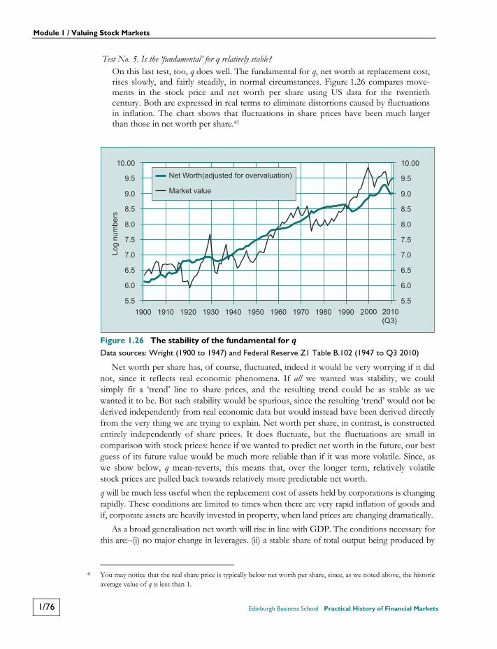
Module 1 / Valuing Stock Markets
1/76 Edinburgh Business School Practical History of Financial Markets
Test No. 5. Is the ‘fundamental’ for q relatively stable? On this last test, too, q does well. The fundamental for q, net worth at replacement cost,
rises slowly, and fairly steadily, in normal circumstances. Figure 1.26 compares move-ments in the stock price and net worth per share using US data for the twentieth century. Both are expressed in real terms to eliminate distortions caused by fluctuations in inflation. The chart shows that fluctuations in share prices have been much larger than those in net worth per share.41
Figure 1.26 The stability of the fundamental for
Data sources: Wright (1900 to 1947) and Federal Reserve Z1 Table B.102 (1947 to Q3 2010)
Net worth per share has, of course, fluctuated, indeed it would be very worrying if it did not, since it reflects real economic phenomena. If all we wanted was stability, we could simply fit a ‘trend’ line to share prices, and the resulting trend could be as stable as we wanted it to be. But such stability would be spurious, since the resulting ‘trend’ would not be derived independently from real economic data but would instead have been derived directly from the very thing we are trying to explain. Net worth per share, in contrast, is constructed entirely independently of share prices. It does fluctuate, but the fluctuations are small in comparison with stock prices: hence if we wanted to predict net worth in the future, our best guess of its future value would be much more reliable than if it was more volatile. Since, as we show below, q mean-reverts, this means that, over the longer term, relatively volatile stock prices are pulled back towards relatively more predictable net worth.
q will be much less useful when the replacement cost of assets held by corporations is changing rapidly. These conditions are limited to times when there are very rapid inflation of goods and if, corporate assets are heavily invested in property, when land prices are changing dramatically.
As a broad generalisation net worth will rise in line with GDP. The conditions necessary for this are:–(i) no major change in leverages. (ii) a stable share of total output being produced by
41 You may notice that the real share price is typically below net worth per share, since, as we noted above, the historic
average value of q is less than 1.
10.00
9.5
9.0
8.5
8.0
7.5
7.0
6.5
6.0
5.5
10.00
9.5
9.0
8.5
8.0
7.5
7.0
6.5
6.0
5.5
1900 1910 1920 1930 1940 1950 1960 1970 1980 1990 2000 2010(Q3)
Net Worth(adjusted for overvaluation)
Market value

Module 1 / Valuing Stock Markets
Practical History of Financial Markets Edinburgh Business School 1/77
the corporate sectors. (iii) a stable capital/output ratio. None of these conditions has held entirely reliably in the past: but, on the other hand, they have not been too far from holding.42
1.13.2 Conclusions: the Case for q as an Indicator of Value
Table 1.7 summarises the results of our five tests for q. It can be seen that q satisfies all the criteria necessary to be a valid measure of value. A comparison with previous chapters will reveal that it is also the only indicator that satisfies all five tests. In an important sense, the very fact that all five tests yield positive results for q, and only for q, gives an additional significance to the individual tests. The whole is greater than the sum of its parts.
Table 1.7 and the five key tests for any indicator of value 1. Measurable? Yes. Modest measurement error is systematic, hence
not a major concern.
2. Mean reversion? Yes.
3. Makes economic sense? Yes.
4. Weakly predicts stock returns? Yes.
5. Stable fundamental? Yes.
Even q is, of course, not a perfect indicator. We have seen, however, that the only signifi-cant limitation of q does not relate to q itself, but to the fact that we can only measure it imperfectly. This indeed is the limitation that prevented the use of q as an indicator of value until relatively recently; and which continues to rule it out for markets that do not have economic statistics of such a high quality as those for the United States.
1.14 Key Conclusions and Unfinished Business We have reached our final section. We would certainly not claim that we have covered every single aspect of the subject of stock market value, but we do hope that we have provided you with an analytical framework, backed up with some key evidence, that will enable you to think about the subject systematically. In this final section we aim to do two things: first, to attempt to draw the threads of our arguments together; and second, to point to unfinished business. On this latter score, if you are interested in pursuing the topic, there is plenty of research available that is highly relevant (though, alas, not always accessible to the non-specialist reader) and covers topics we have only been able to present in a rather cursory manner here. But one of the attractions of this subject area is that there are also plenty of unanswered questions, and so plenty of scope for continuing controversy and debate.
42 Since net worth and GDP have grown at least broadly in line, this explains why the ratio of stock market value to
GDP has also been reasonably stable. But the degree of stability has been distinctly less than that of q, since the above conditions have not held precisely.
Module 1 / Valuing Stock Markets
1/78 Edinburgh Business School Practical History of Financial Markets
1.14.1 All Valuation Indicators Lead to q?
In Section 1.8 to Section 1.13 we worked through the merits and demerits of the key valuation indicators, in relation to our five key tests. We saw that the only indicator that passed all five was q. If you are of a cynical turn of mind, you may suspect that, since we have now been putting the case for q for a number of years, and our reputation is to some extent bound up with this indicator, we might easily have rigged the tests to produce the desired result. We have two responses to this.
The first is positively to encourage you to be cynical about our arguments, as you should be about any arguments you encounter. So you should ask yourself to consider again whether the tests themselves are flawed. We don't think they are; but we would certainly not claim to be infallible. The subject is, as we have already noted, fairly new, and still fraught with some degree of controversy. We noted at the outset that there is still no clear consensus in this area. So, by all means read what we write with a degree of cynicism, and think very hard about our approach when you come to read the arguments of those who disagree with us. But you should also ask how their arguments square up to our approach, and if they ignore it, whether they are evading key issues.
Our second response is to note that these five tests have arisen out of our own experi-ence of attempting to arrive at a satisfactory way of valuing stock markets. Since we started looking at stock market value in a systematic way, at the start of the 1990s, the research we have carried out both at Smithers & Co., and in the academic world, has considered dividend yields, P/E multiples, and cyclically adjusted P/E multiples as possible indicators of value. We confess that we have even looked at yield ratios. The defects of all of these led us to look at q, and to an increasingly strong view that this was the right place to be looking. It also led us to look back at these alternative indicators, to try and pin down what was wrong with them. In this process we developed the tests. We did not develop them because q satisfied them; we became satisfied with q because it passed them.
In Box 1.6 we show that, if you attempt to deal with the problems of other available indicators, then the better we dealt with them the closer we get to the signal that q provides, or – in many markets – that q would provide if we had the data, and assuming we could measure it properly (on which more below). Knowing this helps us to understand the limitations of all the available indicators. Indeed, it helps us to understand the weaknesses of measured q itself. Understanding the necessary logical links between alternative valid measures of value means that we can more effectively use different measures as a cross-check against each other.
Thus we show in Box 1.6 that an idealised measure of q and an idealised measure of the cyclically adjusted P/E multiple would give exactly the same signal. Where we have data on both, knowing this necessary link can be very helpful. Suppose that q points to a lesser degree of overvaluation than the recorded P/E. The conflicting signals might lead you to conclude that there is simply no way to value stock markets. But a more helpful conclusion is that, however many conflicting signals there may be, there can only be one true signal of value.
At the end of 2002, for example, the implied overvaluation of the US market from q was still of the order of 40–50%, but the P/E multiple on the S&P 500, at around 30, was well over twice its historic average. (If you look back at Figure 1.16 you'll see that the P/E actually rose in the early part of the bear market.)
If we know that there can be only one true signal, we have to face up to this, and explain the difference.

Module 1 / Valuing Stock Markets
Practical History of Financial Markets Edinburgh Business School 1/79
Suppose we are pessimistic, and wish to argue that the P/E gives the truer indication of value. We must therefore be arguing that profits are cyclically normal, and investors are demanding the same underlying return as they have demanded historically. Then this must straightforwardly imply that the data on q are badly wrong. Since we know that the top of the ratio is pretty well measured, the bottom must be wrong. If the market is really twice, rather than 1.5 times, overvalued, it must imply that corporate net worth is over-stated by at least one third. But since corporate net worth is simply the cumulated value of retained profits, this must imply that somewhere along the lines profits have been very badly overstated. Hence they may still be today, implying that the true P/E is even high-er, implying in turn an even bigger discrepancy needing to be explained…
Alternatively (and to us, distinctly more plausibly) suppose we wish to argue that q measures the true degree of overvaluation. Since q and the correctly cyclically adjusted P/E must give the same signal, this must imply that the difference between the apparent overvaluation from the unadjusted P/E and that from q is explained by temporary cycli-cal factors in reported profits, which must accordingly be only around two thirds of their cyclically adjusted level.
1.14.2 Living Without q
By this stage you might well be inclined to complain that this is all very well, but since q can currently only be well measured in at best a few stock markets, does this mean that stock market value can be discussed onlyfor those few markets where we can measure q? We would not wish you to draw this conclusion.
It is true that we wish there were more data available on q. Indeed, it is somewhat frus-trating to know that, somewhere out there, in the sea of information on stock markets and related series that has already been collected, the data for q almost certainly do exist already potentially for many other markets; the various sources of data just need to be collated, and examined systematically. We hope, and indeed strongly suspect, that over the next few years the necessary research will be carried out to enable us to discuss q in far more markets.
But in the meantime, even in the absence of good-quality data, we would argue that just the idea of q helps you to understand the concept of stock market value, and to be aware of the potential and actual weaknesses of alternative indicators of value that may currently be available. One of the conclusions to draw from the analysis of Box 1.6 is that, when we only have P/E data, for example, the closer we can get to an economically meaningful cyclical adjustment process, the closer we’ll get to true q, and hence to a sensible indicator of stock market value. Box 1.6: ‘ -Equivalence’: Do All Valuation Indicators Lead to ? _____ We have seen, since we introduced the Dividend Discount Model in Box 1.1, that we can look at all possible valuation indicators in the context of that model. We saw in Boxes 1.2 and 1.3 that this revealed the severe weakness, in terms of mean reversion assumptions, of the dividend yield; and Box 1.4 showed the silly nature of the assump-tions that need to be plugged into the model if you were to attempt to justify the use of yield gaps or yield ratios. We also saw that, in dealing with the problems of both approaches, we were led towards the P/E. Unfortunately this in turn has practical problems, owing to the volatility of earnings (requiring cyclical adjustment) and a degree of weakness, in terms of underlying economics, that we need to assume that investors always demand the same return. Box 1.5 showed that q is not prone to either of these problems, and hence can be criticised only on the basis either of mismeasurement of corporate net worth, or a massive shift in monopoly power.

Module 1 / Valuing Stock Markets
1/80 Edinburgh Business School Practical History of Financial Markets
There is a final stage in our argument that we shall look at here. This is to show that, if we deal with the two key problems of the P/E in a consistent way, we end up with exactly the same signal on overvaluation as we get from q. First of all, let's use a simple application of two of the oldest mathematical tricks in the book. The first is that any expression multiplied by 1 is left unchanged, and that the number 1, in turn, can be written as a ratio of anything to itself: i.e., / 1. The second is that multiplying by a ratio is the same as dividing by the same ratio turned upside down. Using both these tricks, we can express the P/E as
The last expression can then be rewritten, in terms of the definitions, of q and , the return on net worth, from Box 5, as
So what we have shown is that the P/E can be broken down into two components: q, and the return on net worth. This helps us to understand the problems of the P/E, since it shows that it is driven both by changes in q, and by changes in underlying profitability. In the early 30s, for example, q was very low, but the P/E was high, because profitability was so poor: hence was very low, thus massively distorting the signal from q. The cyclically adjusted P/E attempts to deal with this by replacing actual earnings per share with their cyclically adjusted value. But the problem, as we saw, is to know what this value is. One solution that makes economic sense is to assume that, in equilibrium, firms should make an underlying return equal to some equilibrium value. Don't worry, for now, where we get this value from (though if you are on the ball you may already have guessed). This would suggest that we could produce a cyclically adjusted measure of earnings per share defined by
Now let's use the resulting cyclically adjusted measure of overvaluation we proposed in Box 1.3, as the ratio of the cyclically P/E to what it should be in equilibrium, namely Siegel's Constant turned upside down (so to simplify matters we are ignoring any bias in measured profits), i.e. /
/
/
1/
/ .
1/
So the only difference between the measure of overvaluation from the cyclically adjusted P/E, and from q, is the ratio of two returns, the return on net worth and Siegel's Constant. We don't know what these returns are, but this doesn't matter. As we saw in Box 1.5, we have very strong economic arguments indeed to assume that, in a reasonably competitive economy, they must be the same, since the return of capital should equal the cost on capital. So we simply get /
/!
showing that, as long as we do cyclical adjustment in this economically sensible way, the resulting adjusted P/E is ‘q-equivalent’. Since we saw that, when we dealt with the problems of the other indicators, these in turn led us to the cyclically adjusted P/E, these other measures, too, must be q-equivalent: i.e., in dealing systematically with all their problems, we end up in all cases with q. __________________________________________________________________________________________________________________________________________________________________________________________________________________________________________________________________________________________________________________________________________________________________________________________________________________________________________________________________________________________________________________________________________________________________________________________________________________________________________________________________________________________

Module 1 / Valuing Stock Markets
Practical History of Financial Markets Edinburgh Business School 1/81
We saw in Box 1.5, that q still mean-reverts even if Siegel's Constant is not constant. By implication, once we've correctly cyclically adjusted the P/E, the resulting indicator of value must also mean-revert. How does this work? We saw in Box 1.3 that if were to fall permanently, the equilibrium P/E would rise. But since we know would have to fall too, the resulting change in cyclically adjusted earnings per share would precisely offset the change in the equilibrium P/E multiple.
Even when we don't have q data, this result still gives us some insight, since we know that the observed P/E (usually much more readily available) must be made up of the unobserva-ble true value of q, plus the also-unobservable true cyclical adjustment. But we know that the better the cyclical adjustment process is, the closer we’ll get to true q, and hence to a plausible measure of overvaluation.
We should, finally, mention one assumption that we've needed to make to get this result: that we can, effectively, treat net worth per share, W, as unaffected by q, and hence as ‘exogenous’. Statistical evidence suggests that, historically at least, this is a pretty reasonable assumption.43 In our final box, Box 1.7, we shall examine the possibility, based on the EMH, that, despite the evidence from the past, investors might rationally have expected W to do the adjustment. We shall see that the necessary adjustment process would defy not only historical evidence, but also economic logic.
1.14.3 Is the EMH Dead?
We have our personal views on this, on which more below. But whether we are right or not, what is for certain is that proponents of the EMH don't think it's dead.
When we discussed, in Section 1.6, the statistical evidence against the early assumption that stock returns were entirely unpredictable (implying, if true, that statements about value are meaningless), we used our words carefully: we said that the Random Walk version of the EMH was rejected by the data. When this evidence first began to emerge, it was initially viewed as a fatal blow to the EMH. But it could not be killed off so easily.
Cynics might argue that this was because there were so many academics whose profes-sional lives were bound up with the EMH that it would have been disastrous to let it die. Those of a less cynical disposition might argue that the EMH was such a powerful idea that academics were correctly being cautious in not immediately jumping to conclusions and killing it off with undue haste. Whatever, the reason, though, rumours of the death of the EMH have, to paraphrase Mark Twain, been greatly exaggerated.
How could the EMH survive the death of the Random Walk Hypothesis? As it turned out, in terms of logic, at least, quite easily. To quote from a bestselling graduate textbook,
…any test of efficiency must assume an equilibrium model that defines normal security returns. If efficiency is rejected, this could be because the market is truly inefficient or because an incorrect equilibrium model has been assumed. This joint hypothesis problem means that market efficiency as such can never be rejected. (Campbell, Lo and MacKin-lay, The Econometrics of Financial Markets, 1997)
43 See Robertson and Wright ‘What does q predict?’, cited earlier.
Module 1 / Valuing Stock Markets
1/82 Edinburgh Business School Practical History of Financial Markets
The problem the authors are alluding to is that the Random Walk Hypothesis was made up of two elements. First, that markets are efficient. Second, crucially, that the typical investor's expected return is constant – in effect, that Siegel's Constant is not just constant on average over long periods, but in every single period.
There is no particular reason, in logic, for this to be the case. We have already acknowl-edged that even the long-term constancy of investors' expected returns is not all that easy to explain in terms of theory. By implication there is even less reason for theory to predict that it should be strictly constant.
So the response of adherents of the EMH to the apparent knock-out blow caused by the rejection of the Random Walk Hypothesis was to regroup fairly rapidly, and abandon the second, but crucially, not the first part of the hypothesis. If you continued to assume that markets are efficient, then the only way you could explain away the evidence that returns were predictable was to conclude that desired returns were predictable. And this was exactly what adherents of the EMH generally did.44
But there are two major problems with this approach. The first is that, as a result, it has become increasingly accepted that the EMH, in its
revised form, is very close to being untestable. On this basis, the EMH should be rejected, not because it has been falsified by the evidence, but simply because (at least according to its proponents) it never can be falsified.45 This point can be illustrated by a comparison with ‘creationism’ – i.e. the belief that the world was created in accordance with biblical descrip-tions. This view conflicts with the evidence of fossils, which indicates that the world was created rather earlier than 4004 BC, the date derived from the Bible by Archbishop Ussher. To surmount this difficulty, it has been claimed that the contrary evidence has been put on earth by God to confuse the wicked and test the faith of the godly. Clearly no evidence can be produced that can overturn this amended version of the theory. The reason for rejecting creationism, and by implication also to reject the consensus version of the EMH, is not that it can be disproved, but that it simply cannot be tested.46
But the other major problem is that arguably the biggest test of the credibility of the EMH has come about over the past decade or so. The bull market of the 1990s was quite exceptional by any standards. Returns on the way up broke all historical records – not so much in terms of the returns in any given year, but in terms of the sheer length of the period of high returns. As a result, all major valuation indicators reached unprecedented levels. The peak of the boom was thus uncharted territory. As a glance at Figure 1.13, Figure 1.16, Figure 1.18 and Figure 1.24 will show, all measures of value pointed to a significantly greater degree of overvaluation in 1999 even than at the height of the US market in 1929. Indeed, the rise was so sharp that, despite losing roughly half its value by end-2002, we've already seen that q suggested that the US market was still significantly overvalued. For the EMH to remain credible, its defenders had to produce a coherent and plausible explanation of how this could have happened, and in our view they have failed to do so.
44 This is, for example, the line taken in the textbook by Campbell et al from which we have quoted, as also in
Cochrane's Asset Pricing. An alternative approach, taken more recently, has been to argue that the evidence for predictability was in fact spurious. For a strongly expressed argument along these lines, see Goyal and Welch (op cit).
45 ‘I do not demand that every scientific statement must in fact have been tested before it is accepted. I only demand that every such statement must be capable of being tested.’ (Popper, 1959, page 41; italics in original)
46 It is also worth noting once you take this line, the lack of clear statistical evidence against the EMH means that there is an equal lack of statistical evidence in its favour – a point acknowledged by its academic defenders. For example, Hall (2000), a paper we also discussed in Box 1.5.
Module 1 / Valuing Stock Markets
Practical History of Financial Markets Edinburgh Business School 1/83
We have already discussed, in Box 5, one possible defence, which was to argue that the data for q were simply massively wrong, but we argued at the time that this was very hard to defend, since it would imply, in logic, massive mismeasurement of GDP and profits.
The only alternative defence, which we discuss in our final box, Box 1.7, was to fall back on the idea that investors knew that the market was overvalued by historical norms, but were prepared to accept the weak returns that the high level of q was forecasting. But we show in Box 1.7 (which, unfortunately, requires somewhat more maths than the others) that this defence was equally incredible, for two reasons. First, the period in which q must have been expected to fall back to its normal level was implausibly long: anything up to half a century or more. Second, and more fundamentally, because the assumption of perfectly efficient financial markets had to imply that non-financial markets were highly inefficient. Again, we made both these points at the time47– they are not arguments based on hindsight.
Our strong suspicion is that, once the dust settles (and, in all probability, once the US stock market has fallen quite a lot further), the boom of the 1990s, and the subsequent bear market of the new millennium will prove in the end to have been the last straw for the naïve version of the EMH, and economists will begin to look around for something to replace it.48
Box 1.7: EMH Rationales for at the Peak _________________________ For those who wished to argue that the market was efficiently valuing the US corporate sector at the height of the bull market, there were really only two possible explanations of observed values of q. One of these we have already dealt with in Box 1.5: the claim that measured q was radically overstating true q. If you rule out measurement error as a rationale, the only other possible explanation could be if market participants knew that the high level of q implied falls in the share price, and hence weak returns, but were prepared to accept this, because the return they were demanding from stocks was temporarily or even permanently below its historically normal level. A further implica-tion, as we shall show in this box, was that this lower return must also be below the underlying return on net worth during this process. The problem with this argument, as we shall see, is that the implied length of time over which this adjustment towards fair value was assumed to take place was highly implausible.
We first need to think about how q changes over time. Once we've understood this, we can try to work out a possible adjustment mechanism by which q could rationally be expected to fall back to its mean in the end, but during which period, investors could still receive at least as high a return from stocks as from other investments.
To show this, we have to use slightly more complicated mathematical techniques than in the previous boxes. We have tried to keep the explanation as simple as possible, but if you’re not familiar with all the techniques we use, you may have to take some of it on trust. Since / , it follows that
47 Valuing Wall Street, Chapter 28. 48 Defenders of efficient markets have acknowledged the power of events as a test of the theory. Robert Hall (2000)
notes, in his concluding paragraph: ‘This paper has developed a view consistent with the facts. I stress that the view is consistent and is not yet compelled by the facts. We may learn in coming years (for example by a stock market crash) that the high stock market was a mistake…’
Module 1 / Valuing Stock Markets
1/84 Edinburgh Business School Practical History of Financial Markets
where a dot above a variable equals its continuous rate of change over time ( d /d ). Dividing through by each variable means that we are effectively looking at percentage rates of change: so, in words, the equation says that the percentage rate of change in q is equal to the percentage change in P, less that in W. The first of these is quite easy, since we know
the return on investing in stocks is equal to the rate of capital appreciation, plus the contribution from dividends (in this continuous time framework, the same as the dividend yield), which we shall denote δ. It follows that
Net worth increases by retained profits (we ignore revaluations caused by relative price changes):
where E is earnings. In Box 1.5 we used the definition of the underlying return, / , using which we can write (applying some of our usual tricks)
Finally, by subtracting this from the expression for the percentage change in price we get
1
where the last approximation follows if we are measuring ‘true’ q, which has an equilibrium value of 1, and we are not too far away from equilibrium. So, to a reasona-ble approximation, the percentage change in q is simply equal to the difference between two returns: R, the return from investing in stocks, and the underlying return generated by the assets the firm earns, . Thus, for example, the massive rise in q in the 1990s happened because the returns investors were earning were massively higher than the underlying returns on the assets that firms (and really the investors themselves) actually owned. The only way, accordingly, that q could fall back was through a period during which the reverse happened: investor returns had to be less than underlying returns.
This is of course exactly what actually happened: the terrible investor returns over the last few years have unwound a significant part (but, as of mid-2003, not all) of the rise in q over the 1990s. The problem for the EMH is that, if markets were pricing the US corporate sector efficiently at the peak of the boom, investors could not have been expecting such poor returns.
As we have seen, historically investors seem to have required a return of around 6% in real terms. One argument during the boom was that, in future, investors would require lower returns, possibly on a permanent basis. But since, at the time, perfectly safe indexed bonds were offering around 4% in real terms, this effectively put a floor on the minimum returns that investors could have been expecting. The problem with this explanation was that, with such a high initial value of q, this had to imply either that investors were expecting extremely high underlying profitability on a permanent basis (an idea that we have already dismissed as requiring a massive rise in monopoly power), or that the adjustment process was going to take an extremely long time.

Module 1 / Valuing Stock Markets
Practical History of Financial Markets Edinburgh Business School 1/85
To quantify this, we have to do a little more maths. Let's assume, to make things as simple as we can, that the difference between the two returns that determines the change in q was expected to be constant until q got back to its equilibrium value of 1 (we've been assuming from the start that q is ‘true’ q). Let's assume also that this was expected to happen at a date T years in the future , at which point the two returns switch to their equilibrium values. We don't need to know what these are, but we do know, from Box 1.5, that they must be the same, hence q will stop changing, and the equilibrium will be maintained – irrespective of whether there is any permanent change in returns.49 If we take the approximate version of the expression for / this gives us a differential equation in q which, given our other assumptions, can be shown to imply the particular solution
e
where 0 is the value of true q at the peak. If was expected to be above R for the entire adjustment period, this could in principle be consistent with the initial value of true q being above 1.
The problem is: just how long would this take, for realistic values of ? To find out, we need to solve the equation for T (by taking logs of both sides) to give
ln
At the peak, q was close to three times its mean value, so, rather conveniently, for purposes of computation ln 1 since the base for natural logs is e = 2.718). Hence if, for example, the gap between the returns during the transition process was expected to be 2 percentage points, the adjustment process would have been expected to take roughly 1/0.02 50 years! Even if the gap had been expected to be a full ten percentage points, it would still have taken roughly 1/0.1=10 years.
The sorts of differences in returns we are talking about might not seem that big, but you should bear in mind two closely related points. First, we know that in equilibrium the two returns must be the same, owing to competition. We have assumed, just to make the computation as simple as we could, that the difference was constant until equilibri-um was actually reached, but it would be much more realistic to assume that actually the difference would fall away over time towards its equilibrium value of zero. But if this were the case, for the average difference to be as high as we’d assumed, at some point (presumably early on) the actual difference would have to be well above this average figure, to offset the impact of later lower values on the average during the transition as a whole.
The second point reveals a deep internal inconsistency in the EMH. There is no escaping the logic that, according to the EMH, rational investors either had to be expecting (relatively) small differences in returns for an extremely prolonged period, or much bigger differences over a somewhat shorter period. Financial markets are assumed to be perfectly efficient, through the process of arbitrage. But such differences in returns imply that arbitrage outside financial markets must be extremely weak. Imagine a full half-century, during which investors in real assets systematically got higher returns than
49 If you don't like these assumptions, and worry about their impact, very similar results can be arrived at in a more
complicated model. See, for example, Michael Kiley ‘Stock prices and fundamentals in a production economy’, Federal Reserve Board Finance & Economics Discussion Paper 2000–05.

Module 1 / Valuing Stock Markets
1/86 Edinburgh Business School Practical History of Financial Markets
those who invested in the stock market. Or a decade in which they got massively better returns. Either would imply that there would be a massive incentive to get out of stocks, and invest in real assets – a massive arbitrage opportunity, in other words – that, for some reason, EMH proponents had logically to assume would be ignored. So in this context the EMH should really be called the EFMBVINFMH: the Efficient Financial Markets But Very Inefficient Non-Financial Markets Hypothesis. Somewhat cumber-some, we must agree, but far more accurate a description! __________________________________________________________________________________________________________________________________________________________________________________________________________________________________________________________________________________________________________________________________________________________________________________________________________________________________________________________________________________________________________________________________________________________________________________________________________________________________________________________________________________________
1.14.4 Beyond the EMH: Value and Arbitrage Efficiency
If the EMH, at least in its naïve form, is, as we believe, dead, or at best moribund, what should be put in its place? Can we provide an alternative explanation of the central idea that we have presented in this module, which is that markets can, in a meaningful sense, be valued?
One approach is to abandon not just the EMH but the fundamental assumptions of ration-ality that gave rise to it. If we are prepared to believe that the typical investor is just plain stupid then we can interpret indicators of value as allowing us to exploit this stupidity. In this interpretation, smart investors can gain, in using indicators of value, because other investors are predictably stupid.
We do not subscribe to this view. One fool may, indeed, be born every minute. But typically the assumption that you can keep on exploiting the foolishness of this regular supply of fools, in a systematic and predictable way, turns out to be just another piece of foolishness in itself. The Efficient Markets Hypothesis arose out of the very idea that, if you can make money out of something in a predictable way, someone will exploit it. We do not dispute that key idea. And, on the basis of our own personal experience, we would say that there are plenty of people who work in financial markets who are very far indeed from being fools. What we do dispute is that their actions will necessarily result in prices that perfectly reveal value.
In this view, we should stress, we have virtually all economists on our side, at least as a point of logic. Indeed, it was established more than 20 years ago that the perfectly efficient market is a logical impossibility. If trading and seeking information about value were pointless, because value was perfectly revealed by prices, no rational person would do either. It would thus be impossible for prices to reflect all information.50 This conclusion has never been contested.
The issue that economists do debate is not whether markets actually are efficient, but whether they can be treated as if they were: in effect, whether the degree of necessary inefficiency that is needed to reward those who seek out information is small enough to be viewed as negligible.
We accept that the EMH may be a useful way of looking at a wide range of financial markets. The opportunity for effective arbitrage is a necessary and generally sufficient condition for efficiency. Where arbitrage is possible at low risk, markets should approach perfect efficiency. Thus, for example, markets for forward contracts on foreign exchange transactions, or on highly liquid government bonds, where information is relatively easy to find and arbitrage is relatively risk-free, should be highly efficient, and there is plenty of evidence to suggest that they are.
50 Grossman and Stiglitz (1980) On the Impossibility of Informationally Efficient Markets, AER 70, pp. 393–408, Smithers
(1978) also pointed out the paradox.
Module 1 / Valuing Stock Markets
Practical History of Financial Markets Edinburgh Business School 1/87
But we would argue that similar conditions do not apply to the US stock market as a whole. Despite the powerful evidence for periodic misvaluation of the stock market, it would be extremely risky to try to exploit it for profit. Because the obvious question is: who would exploit it?
In many markets the answer would be: leave arbitrage to the professionals. But in the case of the stock market, the professionals, however intelligent and well intentioned, will typically be the last people to act on information about stock market value. The explanation for this lies in a massive conflict of interest. Indeed, if there were not such a strong conflict of interest, the stock market would never have gone through the boom of the 1990s, since most fund managers would have switched the funds they handled out of the stock market long before things really got out of hand.
The conflict of interest exists between the interests of the fund management businesses and the interests of their clients. As we pointed out repeatedly in earlier chapters, valuation criteria cannot give reliable signals, especially about timing of poor returns. For this reason, even at the height of the bubble the chances of the market falling over a reasonably short horizon like a year were never overwhelmingly high: at worst perhaps around two thirds (although they were much higher over longer horizons).51
Any sensible investor, knowing this balance of probabilities, would have switched out of stocks. If investment managers were acting in the best interest of their clients this is what they should have done too. From the viewpoint of those running fund management businesses, however, things looked very different. These businesses are highly valued by the stock market. They are valued in terms of the amount of money they manage rather than the capital in the business. The goodwill involved in them is huge, and any manager who reduces that goodwill is likely to lose his job very quickly.
For the fund manager, therefore, the risks of going liquid in the boom were simply too high. If they had sold and the stock market had continued going up they would have appeared to have a bad performance record, since other fund managers who stayed in the market would have outperformed them. Remember that a probability of roughly two-thirds that the market will fall over the next 12 months implies a probability of one-third that it will carry on rising. This was too big a professional risk for most fund managers to take. If, on the other hand, having stayed in stocks, the market did go down, the chances were that they would perform no worse than their competitors. So they stayed in stocks, against the better interest of their clients.
The overvaluation of the stock market in the 1990s was not a secret. The reason why fund managers did not sell was not in general because they believed that it was reasonably valued, but because they couldn't take the risks involved.
The failure of market participants to exploit the misvaluations for profit is not therefore evidence of irrationality. We simply cannot expect arbitrage to achieve complete efficiency in valuing the US stock market as a whole. So, for as long as complete efficiency remains just a hypothetical construct, reliable indicators of value will continue to have something very useful to say.
51 For a discussion and explanation of how such probabilities could be estimated, see Robertson and Wright's paper
‘The good news and the bad news about long-run stock returns’ (www.econ.bbk.ac.uk/faculty/wright)

Module 1 / Valuing Stock Markets
1/88 Edinburgh Business School Practical History of Financial Markets
1.15 Glossary Arbitrage
This is the process whereby riskless profits cannot be made in financial markets. Where there are more than three financial assets, there will be more prices between them than there are assets. Some of these prices will be set independently of each other, but the others will be set by arbitrage.
Bond yield ratio
This is a general name for a number of possible relationships between equities and bonds. The comparison may be between earnings or dividend yields, either historic or forecast, and long-, medium- or short-dated bonds.
Book value
The value of an asset shown in a company's published accounts and by extension those of all companies and all assets.
Compound average return
The notional constant percentage return that, if earned over a given number of years, would result in the same total return as observed. Thus, if c is a total return index (with reinvested income), the compound average return over N periods, , is defined by
1100
implying the formula for the return itself as
100∗/
1
Cyclical adjustment
At any time, output or profits will differ from their equilibrium level. The process of offsetting this difference is cyclical adjustment.
Data mining
Spurious results can be achieved, either deliberately or by accident, through selecting data that support the desired conclusion rather than by considering all the relevant data. This is contemptuously known as data mining.
Depreciation
Depreciation is the process of writing down the value of capital to allow for its losing its economic value over time.
Dividend Discount Model
This is process of estimating the value of a share by forecasting its future dividends per share and discounting them to give the present value (see Box 1.1).
Earnings per share
For an individual company, the company's total profits, less net interest, tax and depre-ciation, divided by the number of shares. For a stock price index, the average earnings per share of the constituent companies.

Module 1 / Valuing Stock Markets
Practical History of Financial Markets Edinburgh Business School 1/89
Efficient Markets Hypothesis (EMH)
This hypothesis holds that the market price of assets is always correct, and that price changes arise only from new information. Price and value are thus the same, and no profits can be made, other than by chance, without inside information.
Employee stock options (ESOs)
Options to purchase shares in companies granted to their employees, particularly the senior management.
Endogenous
Economic models distinguish between inputs that can be taken as given, as they are determined outside the system (exogenous), and those that are determined within it. The latter are endogenous, i.e. born within.
Equities
The risk capital of firms is variously called equities, or shares in the UK and, most usual-ly, stocks in the US. Note the scope for confusion with the term equity, which is typically used to refer to corporate net worth.
Equity risk premium
This is the additional return that investors expect to receive as a reward for taking the risk of owning equities.
Exogenous
The opposite of endogenous (see above).
Gordon Growth Model
Alternative name for the Dividend Discount Model.
Hindsight value
An estimate of stock market value, at any given time, based on subsequent returns at a range of investor horizons. See Section 1.5.
Historic cost
Term used in accounting to describe balance sheet items recorded at their cost at the time of purchase, rather than at their current replacement cost. With inflation, replace-ment cost will usually be higher than historic cost.
Log returns
An alternative measure to the standard return is the log return, defined by
ln1100
where is as defined below (under return), and ln() indicates logarithms to base e (=2.718281828). A convenient property is that, for returns that are not too positive or negative (roughly speaking, up to around ±20%),
100
but, unlike standard returns, a log return of −x is precisely reversed by a subsequent log return of +x. (In contrast, think about what happens if the value of an investment first falls by 20% and then rises by 20%.) Note that in US, and increasingly UK, usage the terms ‘log’ and ‘ln’ are frequently used interchangeably, but the former term is still
Module 1 / Valuing Stock Markets
1/90 Edinburgh Business School Practical History of Financial Markets
sometimes used to indicate logs to base 10 – a cause of frequent errors in calculations in Microsoft Excel, for example!
Log scale
A chart where equal increments on the horizontal axis correspond to equal changes in the logarithm (to whatever base) of the series being plotted. A convenient resulting property of log scales is that equal percentage changes imply the same rise or fall in the series plotted, in contrast to a standard scale, where the higher the initial value of the series, the larger is the implied rise or fall for any given percentage rise or fall.
Mean reversion
If you look far enough into the future, the best guess for the value of a mean-reverting series will be its historic mean. It thus has a greater than even probability of falling when it is above its historic average, and a greater than even chance of rising when it is below average.
Miller–Modigliani Hypothesis
In essence this hypothesis holds that an asset cannot become more valuable by being partly financed by debt rather than wholly by equity. It is obviously true but causes prac-tical difficulties through the misuse of the Dividend Discount Model. The difficulties arise from the fact that debt is a cheaper form of capital than equity, particularly as in-terest is usually favoured by tax regimes. Thus highly leveraged companies will, ceteris paribus, have higher earnings than less leveraged ones. See discussion in Box 3.
Net worth
The value of a firm's tangible assets, less its net liabilities. By definition the change in net worth should be equal to its retained profits, plus any revaluation of the replacement cost of its assets.
Price-earnings ratio (P/E)
For an individual company, the ratio of a firm's market value to its company's total profits, less net interest, tax and depreciation (or, equivalently, the ratio of its stock price to its earnings per share). For a stock price index, the average (usually value-weighted) of the P/Es of the constituent companies.
Random
If something has any element of unpredictability, it is, in standard statistical terminolo-gy, a ‘random variable’. This applies even if the element of unpredictability is very small. The term ‘random’ is, however, often used to denote something that is entirely unpre-dictable (other than by its historic mean), usually by association with the commonly used term random walk.
Random Walk
If your best forecast of the value of something tomorrow, or in a year's time, or in ten years' time, is its value today, it is a ‘random walk’. A random walk can be written math-ematically as
where is a ‘white noise’ error term, such that 0; , 0 for all non-zero values of i. Hence for any i. An early prediction of the Efficient Markets Hypothesis was that the stock price should be a random walk (see Section 1.6)

Module 1 / Valuing Stock Markets
Practical History of Financial Markets Edinburgh Business School 1/91
Replacement cost
The notional cost of any asset if you were to replace it at current market prices (as op-posed to historic cost).
Return
The return on any asset is defined by 1100 1
where is the price of the asset, and is any income received during year t (for ex-ample, a dividend in the case of a stock, but also in principle interest payments on a bond). It measures the percentage increase in wealth of a notional investor who held all their wealth in the asset in question. We usually measure returns in real terms – i.e., both the price and the dividend are adjusted for the impact of inflation by dividing by some price index (usually the consumer price index).
Stock price
For an individual company, the total value of the company divided by the number of shares (when the number of shares changes due to arbitrary stock splits, etc., the stock price is usually left unaffected). For a market index, a weighted average (usually value-weighted) of the share prices of the constituent companies.
Value-weighted
Averages are weighted averages, where the weight applied to any company's stock price, or earnings per share, etc, is its market value, divided by the total market value of all the companies in the index. By definition, the resulting weights must add up to one.
Review Questions
1.1 A friend tells you that the price of a cup of coffee in ‘The Wild Knight’ (his local night-club) is a bargain at £5. Another tells you that the coffee costs £1 at the railway station and is extortionate. a. Do these statements contain useful objective information or simply represent the biases of
your two friends? b. How would information about the price of cups of coffee in the next station down the line
and in a competing night-club, ‘The Bad Baronet’, help you decide on the presence or absence of bias in your informants?
c. What other information would you like to have before submitting your report on the values to the Coffee Consumers Guide?
1.2 You are sitting on the trading desk of a large international bank, which can borrow over the short-term at the risk-free rate of interest. Your screen shows the following: 1 year US risk-free interest rates 3%; 1 year UK ditto 5%.
US$1.7 = £1 spot and also the same price for the 1 year forward rate (in which buyer and seller commit to a price for a transaction to take place in one year's time).
a. What action would you take? b. Why would you not expect this situation ever to recur?

Module 1 / Valuing Stock Markets
1/92 Edinburgh Business School Practical History of Financial Markets
1.3 A friend points out that, while individual investors can realise capital gains by selling shares, they can do this onlyby selling them to somebody. He therefore claims that investors in aggregate can't sell and can't therefore make realised capital gains. He therefore claims that the stock market is just a casino, as investors are in it to realise capital gains, while dividends are the only real source of cash for investors in total.
How would you seek to persuade him otherwise?
1.4 You are asked to advise several people on a sensible investment policy for them. They have already taken such excellent tax advice that none of them will pay any tax. You know that the stock market is neither expensive nor cheap, and that its long-term return is thus likely to be the historic average return of 6.7% in real terms. Ten year index-linked bonds yield only 4% and cash 2%. You also know that the life expectancy of a 64 year old man is 15 years. What policies would you recommend, and why, for: a. A 64 year old man who plans to buy an annuity in one year's time? b. A 64 year old man who has no wife or children and no one to whom he wishes to leave
money? c. A 20 year old man who is starting to make contributions to his defined contributions pension
fund?
1.5 Annual percentage returns from the equity market have the following pattern over six years:
10%, 0, 6%,−3%, 4%,−13%, 13%, 18%.
a. Suppose investors expected returns of 5% per year. Calculate their implied prediction errors in each year.
b. Now assume they expected returns of 8%, and do the same calculations. c. Do the prediction errors ‘cancel out’ in the two cases?
1.6 We argued that the average real return on the US stock market over the twentieth century might overstate the average of the true expected return of the typical investor in global stock markets over this period. a. Can you think of an equivalent reason why, for example, the average returns on the French
and German stock market might understate expected returns? b. The Dimson database omits several markets that were important in 1900, but much less
important in 2000 – for example India and Argentina. Would you expect the omission of these markets to bias the estimate of global expected returns upwards or downwards?
1.7 Look back to the sequence of returns in Question 1.5. a. Calculate all possible two-year compound average returns, and verify that the variability (e.g.,
standard deviation or range) thereof is less than that of the one-year return. b. Which will be more volatile: the compound average return over 40 years, or the ‘average
horizon return over 1–40 years’ used in Chart 11.5? Explain your answer.
1.8 We argue that we shall need a lot more data to be able to substantiate our guess that 1999 will prove to have been the worst year to buy stocks in the entire twentieth century. a. Explain why. b. Discuss what evidence you would need to substantiate the claim that 1999 was clearly a good
year to have sold US stocks. (Hint: do you need hindsight?)

Module 1 / Valuing Stock Markets
Practical History of Financial Markets Edinburgh Business School 1/93
1.9 It used to be thought that stock returns were entirely random. (This is typically expressed as the Random Walk Hypothesis, since cumulative total returns will follow a random walk.) Explain whether the following statements are consistent with that hypothesis: a. The long-term real return on equities in the past was 6.7%. We are therefore justified in
assuming that this is the best estimate we can make of the likely return from investing in the stock market today.
b. Equity investment should be for the long term, and investors should buy and hold rather than try to time the stock market.
1.10 a. Why do you think that ‘expectational (aka prediction) errors’ are likely to be greater or
smaller for investors in index-linked bonds than for those investing in equities? b. Do you think that expectational errors are likely to be greater or smaller for investors in
indexed linked bonds than for those investing in nominal fixed rate bonds? c. How would you compare the probabilities of ‘expectational errors’ in equities and nominal
fixed-rate bonds?
1.11 You attend a presentation on asset management in which a new stock market valuation criterion is presented. The following claims are made by the analyst doing the presentation: i. By using this criterion you can spot when the market is about to fall, 95% of the time. ii. This result is based on ten years' worth of data. iii. The analyst shows you a chart of the valuation criterion. It looks like Figure 1.12. He says: ‘My
criterion is at an all-time high: this means the market is going to fall next year.’ iv. He shows you a chart of the fundamental, which fell by 30% in the most recent year. v. When asked about how he arrived at his chosen measure of the fundamental, he answers: ‘I
did a thorough review of available economic data, and looked for series that seemed to pre-dict stock prices. My fundamental is a weighted average of these series.’
Criticise his presentation on the basis of the criteria set out in Section 1.7.
1.12 Figure 1.13 shows that, for most of the nineteenth century, the dividend yield was typically around 6%.
Given what you know about Siegel's Constant from Section 1.4, what can you infer about the typical rate of capital appreciation on the US stock market during this period?
1.13 ‘All you need for an indicator of stock market value is that it should be reasonably stable, so that when the stock market rises or falls, the market gets cheaper or more expensive. Anything that is stable will do.’ a. Criticise this statement on the basis of the evidence in Chart 8.3.
1.14 You are given the following reliable pieces of information for the world economy. (i) Company leverage (the amount of debt finance relative to equity finance) will be stable in the future. (ii) Siegel's Constant will be constant at 6.7% p.a. (iii) The share of corporate output in the whole economy will be stable, and the amount of capital that must be invested to get a given increase in output will also remain stable. (iv) Future GDP growth will be 2.5% p.a. a. What would you conclude about the average dividend yield in the future? b. What could you conclude about the average cashflow dividend yield? c. Assuming that all cash paid out to shareholders was via traditional dividends, what would the
average payout ratio be?

Module 1 / Valuing Stock Markets
1/94 Edinburgh Business School Practical History of Financial Markets
1.15 In both the late 1920s and the early 1970s, the cashflow dividend yield was significantly lower than the standard measure.
Explain the mechanism by which this must have occurred.
1.16 The historic average P/E multiple is around 13, which corresponds to an earnings yield of 7.7%. a. Why would you expect this to be similar to Siegel's Constant?
While it is not dissimilar it is somewhat higher. b. Explain why this is probably the result of habitual overstatement of profits.
1.17 Using the analysis of Box 3 (Section 1.10), explain why, if Siegel's Constant really is constant. a. The P/E multiple must be mean-reverting, as long as any over- or understatement of reported
earnings per share is systematic (i.e., measurement error is itself mean-reverting – see answer to Question 28).
b. Habitual overstatement of profits results in a lower P/E than you would expect, given the evidence on Siegel's Constant.
c. A permanent change in the payout ratio (p) will cause a permanent change in the dividend yield, but not in the earnings yield or p/e multiple.
1.18 The P/E multiple mean-reverts, but the fundamental (E) is highly volatile.
What would you expect to be the effect of averaging E over a number of years in terms of both mean reversion and volatility?
1.19 a. Would you expect dividends to grow faster or slower in nominal terms, if inflation picks up
over the longer term? b. Would this make shares more or less valuable? c. Would you expect interest rates to fall or rise, if inflation were to fall over the longer term? d. Would you expect this to make shares more of less valuable? e. Which of these arguments is fundamental to the bond/yield ratio?
1.20 The long-term average value of equity, q, is around 0.65.
If on 31 December 2005 it were to be 1, what would you conclude about the market? Would it be correctly valued, cheap or expensive?
1.21 a. Why did academic economists previously assume that q must have predictive power for
investment, rather than changes in stock prices? b. During the 1990s boom, critics of q frequently claimed that the mean value of q would in
future remain permanently higher. If this were the case, what would be the implications for the relative magnitudes of the cost of capital and the return on capital?
c. If (as discussed in Box 1.5, Section 1.13) corporate net worth in the 1990s had been as massively understated as some claimed, explain why this must have implied major mis-statement of profits in earlier years. (Hint: think about what causes corporate net worth to change.)
1.22 Equities are (i) financial assets and (ii) titles to real assets. a. Describe the benefits that investors receive from holding financial assets and the way,
common to all such assets, in which they can therefore, at least in theory, all be valued. b. Describe the way in which the price of real assets is determined in a competitive economy and
how, therefore, the value of the stock market will be determined under competitive conditions.