Practical hints for using numerical methods in rock mechanics · Practical hints for using...

Editor: Prof. Dr.-Ing. habil. Heinz Konietzky Layout: Angela Griebsch

TU Bergakademie Freiberg, Institut für Geotechnik, Gustav-Zeuner-Straße 1, 09599 Freiberg [email protected]

Practical hints for using numerical methods in

rock mechanics Author: Prof. Dr. habil. Heinz Konietzky, (TU Bergakademie Freiberg, Geotechnical Insti-

tute)

1 Introduction ............................................................................................................. 2

2 Initial- and Boundary Conditions ............................................................................. 2

3 Meshing Rules ........................................................................................................ 4

4 Meshing Techniques .............................................................................................. 5

5 Model Size .............................................................................................................. 7

6 Continuum versus Discontinuum – Scale Effects ................................................... 8

7 2D versus 3D ........................................................................................................ 10

8 Specifics for Simulation of Dynamic Processes .................................................... 11

9 Mesh dependency in the post-failure region ......................................................... 13

10 Parallel computing ............................................................................................. 14

11 Choice of numerical method / code ................................................................... 16

12 Conceptual and numerical model ...................................................................... 18

13 Important terms .................................................................................................. 23

14 Current and future trends ................................................................................... 24

15 Literature ............................................................................................................ 24

Practical hints for using numerical methods in rock mechanics

Only for private and internal use! Updated: 8 December 2016

of 25

1 Introduction

Although numerical software products become more and more easy to handle and find broad acceptance and use in engineering practice as well as in geo-engineering sci-ences, careful choice and use of these powerful tools are necessary to avoid wrong calculation results. Quite a lot of aspects have to be considered, like:

Choice of appropriate numerical technique and tool Initial and boundary conditions Appropriate model size Choice of appropriate constitutive models and parameters Meshing (structure, density, element type) and mesh-dependency 2D versus 3D Coupling (hydro-thermal-mechanical) Modelling sequence Continuum versus Discontinuum approach Calculation efficiency versus accuracy Static versus dynamic simulations

Also, different solution schemes (implicit versus explicit), different element-types, dif-ferent couplings etc. often need application of special simulation procedures. Therefore, careful inspection of model set-up and in-depth analysis of simulation re-sults is necessary. Comparison with other methods and experience or measurements is strongly recommended.

2 Initial- and Boundary Conditions

The solution of differential equations (both, analytical and numerical) requires the spec-ification of initial and/or boundary conditions. Boundary conditions describe time-inde-pendent or time-dependent mechanical, thermal, hydraulic, chemical … conditions, which are applied to inner or outer boundaries. Initial conditions describe mechanical, thermal, hydraulic or chemical … conditions at the begin of the simulation (at zero point in time) either at the boundaries and/or the inner model area. Boundary conditions (examplary):

stresses

forces

velocities

accelerations

displacements

water pressures

temperatures



of 25

Initial conditions (examplary):

primary stress state

primary deformation state

primary pore water pressure / joint water pressure

initial temperature distribution Displacement boundary conditions are also called ‚Dirichlet‘ conditions, force and stress conditions, however, are called ‘Neumann’ conditions. For static calculations in geomechanics, depending on the application and modelling task, displacement and stress boundaries are applied. In most cases (not always!) displacement boundary conditions deliver too small deformations inside the model and stress boundary conditions over-predict deformations. However, if boundaries are far enough away from the interesting inner model area both types of boundary conditions deliver similar results (results converge with increasing model size). If analytical rough estimates or practical experience are not available, a preceding pa-rameter study shall be performed to investigate the influence of model size and bound-ary conditions on the results of the specific model.

Fig. 1: Normalized stresses and displacements at two observation points in dependence of the type

of boundary condition and the ratio of model size to excavation size [ITASCA 2011]



of 25

Exemplary, Fig. 1 demonstrates, how displacement and stress values inside the model with two excavations alter in relation to model size. Furthermore, this figure illustrates the influence of the displacement and stress boundary conditions on the results in comparison to the exact analytical solution. One recognizes, that with increasing dis-tance between the boundaries and the inner model area both types of boundary con-ditions converge and come finally close to the analytical solution. Boundary conditions are normally applied in form of normal and/or tangential components or in Cartesian coordinates. Also, over different regions of the boundary different types of boundary conditions can be applied.

3 Meshing Rules

For 2- and 3-dimensional discretization (meshing) of objects, three fundamental as-pects should be considered:

Choice of appropriate element type

Appropriate mesh density

Choice of appropriate meshing technique In principle, it can be distinguished between the following element types:

Volume elements (e. g. triangular or rectangular elements in 2D and tetrahe-dral or squared elements in 3D) – typical for rock mass or massive concrete

Shell elements (planar elements with negligible thickness, but explicit consid-eration of moments and membrane stresses) – typical for shotcrete and thin masonry or concrete walls

Bar elements (1-dimensional elements) – typical for anchors, piles or struts Furthermore, for one element type, different shape functions can be applied, which implies different interpolation functions and finally leads to different accuracy (non-lin-ear interpolation). Two competitive demands have to be considered in respect to mesh density (gridpoint distance):

Mesh density : this leads to improved resolution and higher accuracy, but: this leads, on the other side, to increasing calculation time and storage de-mand

For meshing the following general practical rules are guilty:

Several elements of low order (lineare shape function) give equivalent results compared to less number of elements of higher order (non-linear shape func-tion)

Refined meshing is necessary, whenever high stress and deformation gradi-ents are expected, that means for instance at free surfaces, areas with high stiffness contrasts, areas with support elements or areas with load entry points



of 25

Elements should be designed preferably equidistant, meaning the ratio of maximum edge length to minimum edge length should be smaller than about 10, also very small angles between edges should be avoided

Elements should preferably aligned according to the expected stress trajecto-ries

Transition between coarse and fine meshed areas should be smooth (prefera-bly without discrete jumps in element size)

In general: Quad-elements gives more accurate results than triangular-shaped elements

4 Meshing Techniques

In a broader sense, meshing comprises two phases: set up of geometrical model and subsequent filling with elements (meshing). A distinction is made between:

free meshing: delivers an unstructured mesh, which just satisfies a few gen-

eral user defined criteria (e. g. max. edge length pre-defined value)

mapped meshing: delivers a structured mesh, e. g. adjusted according to the model geometry and/or expected stress trajectories

The following conventional meshing techniques are used:

Generation of geometry (e. g. CAD-based with Boolean Algebra) and subse-quent automatic meshing via free or mapped meshing

Generation via primitives: compilation via several basic bodies filled with ele-ments (already meshed volumes)

Deformation of a basic mesh and extension by copying / extrusion / mirroring

Set-up of model (geometry + mesh) via imported point, edge and element data

Today, 2D meshing with different techniques is unproblematic, performed fast and nearly fully automatic. However, 3D meshing, especially with top-quality cuboidal ele-ments and complicated geometry, like for example tunnel crossings, are still compli-cated to perform, quite time consuming and often manual interaction is necessary dur-ing the meshing process. For 3D models in most cases the following procedure is applied:

Generation of geometrical model with a CAD-Program

Export of CAD model data into a standard format (e.g. IGES, STEP, STL etc.)

Import of CAD geometry into a meshing tool, execution of meshing and export of mesh into a format, which can be used as input for the numerical simulation tool (solver)

Input of mesh into the numerical simulation tool and solving the problem Several of the numerical simulation tools have already integrated CAD tools and mesher. The following Figures 2 – 6 illustrate exemplary some of the above mentioned



of 25

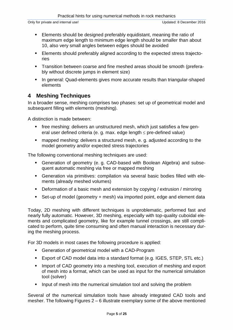
meshing techniques. Remacle et al. (2010) proposed an interesting algorithm for cre-ation of quadrilateral meshes based on prior triangulation (Fig. 6).

Fig. 1: With zones filled basic volumes, which can be composed to a final model (‚LEGO-system‘),

(ITASCA 2012)

Fig. 2: Assemblage of subnets via docking and mirroring

Fig. 4: Generation of final mesh by graduel geometrical adaption and mesh refinement



of 25

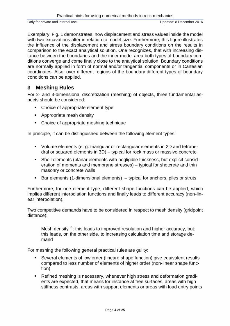
Fig. 5: Generation of final mesh via trimming, deformation and partial deletion of virigin (initial) mesh

Fig. 6: Illustration of Blossom-Quad algorithm: transition form triangulation to quad-mesh (Remacle et

al. 2010)



of 25

5 Model Size

The ratio between model size (overall dimension of numerical mesh) and object size (e.g. dimension of excavation, pillar, slope etc.) plays an important role in respect to correct simulations (see also DGGT 2014). An optimum of two competitive require-ments have to be found (see also chapter ‘Meshing rules’):

Preferably large ratio model size / object size to minimize boundary influence

Preferably small ratio model size / object size to minimize calculation time and memory space.

A second aspect, especially important for settlement and uplift prediction, is the prob-lem, that overall model size has a non-vanishing influence of these deformation values. In case of large overall model dimension elastic or simple elasto-plastic models would lead to unrealistic high deformation values. To avoid these problems either depth-de-pendent stiffness values or so-called ‘small-strain stiffness’ has to be included.

6 Continuum versus Discontinuum – Scale Effects

At a certain scale all geomaterials and construction materials should be considered as discontinua, e.g. sand in form of grains or a fractured rock mass in form of rock blocks as well as composite constructions like tunnel lining / rockmass, anchor / rockmass, geotextile / ballast or pile / wall. Whether discontinuum modelling shall be applied or not, depends on three factors:

Ratio of representativ elementary volume (REV) to total volume

Modelling task (interesting phenomena)

Availability of parameters

Availability of software REV is defined as the smallest volume, from which measurements, parameters and object reactions, respectively, can be obtained and which are representative for the whole rock mass. That means: the REV is the smallest continuum mechanical volume, which is statistical equivalent to the in-situ discontinuum. Fig. 6 shows the history of the two quantities npm and nfr as function of considered volume. One recognizes, that the spread of the quantity decreases with increasing volume (e.g. strength values, deformation module, permeability etc.) und finally the quantity converges and reaches a nearly constant value. Beyond a specific volume Vmin, which represents the REV, the quantity does not change any more significantly even over a bigger volume towards Vmax. Like Fig. 7 also shows, the area of Vmin - Vmax can be quite different for different physical quantities. If several quantities have to be considered simultaneously the common intersection (overlap) have to be considered. In such a case Rfp hast to be considered as REV.



of 25

Fig. 7: Parameter history as function of considered volume (scale effect).

heavy fractured rock mass

many joint sets

two joint sets

single joint set

intact rock

Fig. 8: Relation between structure and considered volume using the example of a rock mass (scale

effect).

Depending on the considered volume the rock mass structure shall be modelled in different ways (8). In case of very small volumes, it is possible that only intact rock exist and therefore a classical continuum mechanical approach with rockmechanical param-eters is recommended. At bigger volumes several single joints or joint sets are ob-served, which can be handled best with a discontinuum mechanical approach (e.g. Discrete Element Method), where different material laws and parameters are assigned to rock matrix and discontinuities in an explicit manner. If a huge number of joints or joint sets exist (highly fractured rock mass), it make sense, to go back to a continuum mechanical approach, where the effect of the discontinuities is not directly (discrete) considered, but in a smeared manner by reduced strength and stiffness parameters.



of 25

But, due to increased computer power today even complex DFN’s can be modelled via DEM-techniques (e.g. Sainsbury 2015). The scale effect is highly important for rockmasses and has to be considered carefully whenever constitutive laws and corresponding parameter are chosen. Rockmass clas-sification schemes can be used to deduce appropriate rockmass parameters based on rockmechanical lab data and engineering-geological investigations according to the following scheme:

Determination of rockmechanical parameters in the lab

Engineering-geological inspection (core analysis, joint-set statistics etc.)

Rockmass classification (e.g. RMR, Q, GSI, RQD) on the basis of the engineer-ing-geological inspection and the rockmechanical lab data

Deduction of rockmass parameters for suitable constitutive laws (e.g. Hoek-Brown, Mohr-Coulomb etc.) on the basis of the rockmass classification

7 2D versus 3D

In the forefront of any numerical model set-up the following key questions should be answered:

Is a 3-dimensional modelling necessary or is a 2-dimensional consideration ac-ceptable?

Are there symmetry lines or planes which would allow to reduce the model size?

A complete 3-dimensional modelling is necessary, if:

the strike of the geological elements (layer, joint, fault, bedding plane …) does not coincide with the long axis of the geotechnical construction

the axes material anisotropy do not coincide with the axes of the geotechnical construction

the directions of principal stresses are neither parallel nor perpendicular to the axes of the geotechnical construction

the dimensions of the geotechnical constructions and the geological bodies, re-spectively, are nearly equal in the three spatial directions

several structural components intersect each other (e.g. tunnel crossings)

applied boundary conditions (forces, velocities, stresses ….) have components in all 3 spatial directions

If symmetry conditions are met, models may be reduced (simplified) to half or quarter models or even reduced from 3D to 2D (axisymmetrical). However, one has to take into account, that symmetry conditions have to be referred to several aspects, which have to be met simultaneously:

in respect to the geometry

in respect to the stress field

in respect to the constitutive law (planes of anisotropy, orientation of joints etc.)



of 25

in respect to the modelling sequenz (construction process, excavation phases, support measures etc.)

in respect to boundary conditions

in respect to support installation- and preservation measures (anchors, shot-crete, piles, struts etc.)

in respect to couplings (hydraulic, thermal etc.) 9 illustrates potential model reductions on the basis of pure geometrical considerations, like used to simulate shaft- , tunnel- and borehole problems or building excavations.

Fig. 9: Examples for model reduction on the basis of the consideraion of pure geometrical symmetry

conditions (full model, half model and quarter model)

8 Specifics for Simulation of Dynamic Processes

The simulation of dynamic processes involves wave propagation and requires the consideration of four important aspects:

The correct representation of movement of waves requires that the maximum gridpoint distance hp,s has to be considerable smaller than the shortest wave

length p,s:

1

1 110 10 S

P P

E

ch

f f

(1)

10 10 SS S

G

ch

f f

(2)

hP: maximum gridpoint distance for P-wave (longitudinal wave / compression wave) hS: maximum gridpoint distance for S-wave (transverse wave / shear wave) cp: P-wave velocity cs: S-wave velocity f: Frequency E: Young’s modulus

: Poisson’s ratio

Model boundaries shall be designed in such a way, that reflections are avoided to a large extent (application of anechoic boundary conditions).



of 25

As a general rule, dynamic strength parameters are higher than static values (e.g. factor of app. 1,5). Therefore, strength parameters have to be adjusted for the dynamic calculation part.

The numerical algorithm has to include physical correct damping for wave propagation. Often applied algorithms are:

o mass-proportional damping

o stiffness-proportional damping

o local damping

o Viscous damping

o Rayleigh damping

o Intrinsic damping (damping due to plastifications) The damping behavior can be described by the seismic quality factor Q. The seismic quality factor is frequency independent and effects increasing damping with increasing frequency, which is characteristic for geomaterials. This requirement is satisfied by the local damping scheme and, for a broader frequency range, also for the popular Ray-leigh damping (Fig. 10).

𝑄 =𝜋𝑓

𝛼𝑐 (3)

where: f: frequency [Hz] c: wave speed [m/s] α: damping coefficient [m-1]

mass proportional

stiffness proportional

Rayleigh

local

Frequency

Damping

Fig. 10: Damping vs. frequency for different damping procedure

The logical consequence is, that normally dynamic meshes shall have much higher resolution (much smaller gridpoint distances). This results in larger computation times. Also, often it is necessary to filter the dynamic input signal to suppress higher frequen-cies and to perform baseline-correction.



of 25

9 Mesh dependency in the post-failure region

The post-failure behavior is characterized by so-called ‘localization’. Localization means the progressive accumulation (concentration) of microcracks within a small macroscopic fracture plane (zone, band). This process is numerically represented by the so-called strain softening, which is dependent on the grid structure (Fig. 11). That means, that the stress-deformation behavior inside the post-failure region is heavily dependent on the mesh resolution. In principal, there are three different solutions to overcome this problem:

Calibration on a fixed grid structure (mesh resolution should be constant for any model using one calibrated data set)

Adaptive re-meshing inside the localization (mesh refinement)

Extension of the constitutive model by internal scaling parameter (regulariza-tion)

a b c da, b, c

, d

Fig.11: Stress-strain behavior with strain-softening and different mesh refinement a,b,c and d without

any procedure to avoid influence of mesh dependency

Similar behavior is sometimes observed, when static problems with pronounced plas-tifications are calculated by using explicit methods and loading or unloading occurs instantaneously. Therefore, in such cases properties, loads or geometrical changes should be performed gradually. Exemplary, Fig. 13 shows displacement magnitudes along the tunnel contour for a model according to Fig. 12 with isotropic virgin stress field, but anisotropic material behavior with complex plastification pattern. As Fig. 13 illustrates, coarse mesh (here: 900 zones) does not deliver correct values, but meshes with number of zones around 14000 or bigger give nearly identical results. Also, with-out soft relaxation of boundary stresses at the tunnel contour (see dashed line in Fig. 13) wrong displacements are obtained. That statement, that appropriate choice of ele-ments and mesh density is essential to obtain reasonable results is supported by a lot of studies, e.g. Batoz et al. (1980), Jovanovic et al. (2010), Ljustina et al. (2014) or Veyhl et al. (2010).



of 25

Fig. 12: Mesh for ¼-symmetric tunnel including boundary conditions (900 zones)

Fig. 13: Displacement magnitudes along tunnel contour vs. location of observation point

10 Parallel Computing

Huge numerical models (huge number of elements, zones, blocks, grid points etc.) demand very long runtimes (days up to weeks). Therefore, parallelizing also called high performance computing (= usage of several processors in parallel) is suggestive. Parallelization can be realized in different ways: e.g. by hyper- and multi-threading (shared memory computing) or physical partitioning of the model to several processors (at best this could be several processors at one board, but also several computers within a network or cluster – distributed memory computing). Shared memory computer reach maximum speed, if all processors on board are used. Further speed increase can be reached if hybrid parallel computing is applied (combination of shared and dis-tributed memory methods).



of 25

However, the calculation speed does not linearly increase with number of processors, but the calculation speed follows Amdahl’s law:

1m

p

s

Sf

fN

(4)

where: Sm factor of speed increase N number of processors fp share of parallelized code fs share of serialized code It holds fs + fp = 1, where fp < 1, because at least the communication between proces-sors has to be performed in a serial manner. Fig. 14 illustrates Amdahl’s law.

S

N

m

Fig. 14: Amdahl’s law: Increase in claculation speed Sm as fuction of number of processors N

To evaluate the efficiency of parallelization, a measure of efficiency can be defined (Fig. 15):

s

n

T

N T

where: Ts calculation time using 1 processor Tn calculation time using N processors N number of processors

1

N

number of zones

Fig. 15: Calculation efficiency η as function of number of processors N and number of zones



of 25

The efficiency of parallelization increases with increasing number of zones and de-creases with rising number of processors.

11 Choice of numerical method / code

Numerical simulation techniques can be distinguished either according to:

temporal discretization into explicit and implicit methods spatial discretization into mesh-based and meshless methods

Whereas implicit methods are faster than explicit methods in case of elastic simula-tions, explicit methods are better suited whenever large deformations, strong non-lin-earities or physical instabilities occur (e.g. crash or impact simulations, blasting, rock cutting or drilling, rockfall etc.) In respect to spatial discretization of mesh-based methods one can further distinguish Finite Element (FE, XFE), Finite Difference (FD), Volume Element (VE) and Boundary Element (BE) methods. The most popular representatives of meshless methods are the Discrete Element Methods (DEM) based on spheres or polyhedra and the Smooth Particle Hydrodynamics (SPH) method. Mesh-based methods can be distinguished into integral (BEM) and differential (FEM, FDM, XFEM, VEM) methods. Integral methods have the following general character-istics:

simple meshing (only at surfaces) exact far-field solution minimized discretization error no problems with singularities small demand of computational power but: problems to handle anisotropies, inhomogeneities, couplings, non-lineari-

ties Differential methods have the following general characteristics:

ability to depict any kind of anisotropies, inhomogeneities, couplings, non-line-arities

tremendous flexibility to solve continuum mechanical problems higher demand for computational power sometimes complicated meshing procedure problems to simulate disintegration and mixture of material

Compared to classical integral or differential methods, meshless methods including DEM are characterized by several additional features:

discrete elements should be able to follow all kinematic possible movements (displacements and rotations)

automatic contact detection and elimination of contacts (e.g. via cell-space or Verlet algorithm)

contact laws, which act, whenever a contact (direct touch or long-ranging inter-action) exist



of 25

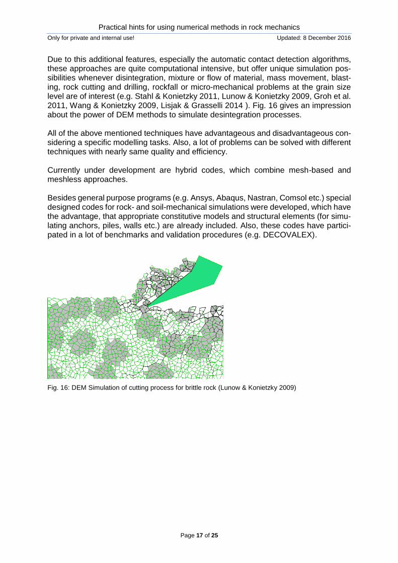
Due to this additional features, especially the automatic contact detection algorithms, these approaches are quite computational intensive, but offer unique simulation pos-sibilities whenever disintegration, mixture or flow of material, mass movement, blast-ing, rock cutting and drilling, rockfall or micro-mechanical problems at the grain size level are of interest (e.g. Stahl & Konietzky 2011, Lunow & Konietzky 2009, Groh et al. 2011, Wang & Konietzky 2009, Lisjak & Grasselli 2014 ). Fig. 16 gives an impression about the power of DEM methods to simulate desintegration processes. All of the above mentioned techniques have advantageous and disadvantageous con-sidering a specific modelling tasks. Also, a lot of problems can be solved with different techniques with nearly same quality and efficiency. Currently under development are hybrid codes, which combine mesh-based and meshless approaches. Besides general purpose programs (e.g. Ansys, Abaqus, Nastran, Comsol etc.) special designed codes for rock- and soil-mechanical simulations were developed, which have the advantage, that appropriate constitutive models and structural elements (for simu-lating anchors, piles, walls etc.) are already included. Also, these codes have partici-pated in a lot of benchmarks and validation procedures (e.g. DECOVALEX).

Fig. 16: DEM Simulation of cutting process for brittle rock (Lunow & Konietzky 2009)



of 25

12 Conceptual and numerical model

Each numerical modelling should be separated into 2 successive phases:

1. Phase: Conceptual model 2. Phase: Numerical model

The first phase comprises the development of the general modeling strategy and in-cludes some more general decisions about simulation tools and approaches. The second phase comprises the programming, specific allocation of constitutive laws, initial and boundary conditions, parameters etc. and the corresponding model runs in-cluding evaluation.

Phase 1: Conceptual model:

Phase 1 starts with an analysis of the modelling task and the available data base fol-lowed by the allocation to the corresponding phase and finally the detailed analysis of all aspects according to Fig. 17. Each geotechnical task can be subdivided into several stages, like:

Pre-planning Dimensioning Construction Monitoring Backanalysis

Besides typical geotechnical project work, applied or fundamental geotechnical re-search work exist. Depending on the project phase, tasks, demands and applications, numerical simula-tions will be quite different. In the pre-planning phase quite often only a very limited data base exist, the budget is limited and the expectations about precision in prediction are lower. Therefore, in this phase numerical modelling is restricted to simplified geometries, coarser meshes, sim-ple constitutive laws and consideration of less construction stages. The pre-planning phase also includes the comparison of different concepts. The aim of this phase is to detect the main geomechanical features / characteristics / pitfalls etc. of the project, to get the correct order of magnitude in terms of stresses and deformations and to obtain a deeper understanding of the geomechanical processes. Also different construction methods can be compared and evaluated. The phase of dimensioning / detailed planning requires a valuable and comprehensive data base. Material behavior and interaction between rockmass and structure have to be described by appropriate constitutive laws in detail. The construction phase is characterized by application of numerical modelling in par-allel to the in-situ construction steps. During that phase the model has to be up-dated, corrected, improved etc. based on actual in-situ measurements and observations. The model is used to interpret / explain observations and can be used to predict the effect



of 25

of short-termed changes during the construction or to perform backanalysis in case of any disaster (failure). The phase of monitoring and backanalysis normally starts, when the construction is finished and characterized by the fact, that in-situ measurement data and observations in respect to the interaction rockmass – construction are available. The aim of model-ling during these phases is the back-calculation of parameters or to analyze failure situations. The approach to perform fundamental or applied research can be quite different and is highly dependent on the modeling task (often innovative approaches). If one has defined the corresponding phase, several aspects according to Fig. 16 have to be considered. Especially, the following questions have to be discussed:

Should the problem be modelled 3-dimensional or is a 2-dimensional approach sufficient or is the assumption of axisymmetry (quasi-3D) acceptable? If so, how can symmetry lines / planes be defined? Please note, that in respect to symmetry not only geometry has to be considered, but also other factors like stress state, anisotropy of material etc.

What is most appropriate way to solve the modelling task: a continuum ap-proach or a discontinuum approach? This is decisive for the choice of corre-sponding software tools.

What type of constitutive model is appropriate (elastic, elasto-plastic, visco-elasto-plastic, fracture mechanical, damage mechanical … )?

Can the simulation be performed as pure mechanical one or should couplings be considered, e.g. hydro-mechanical, thermo-mechanical, hydro-thermo-me-chanical, hydro-thermal-mechanical-chemical … )?

Do we have a pure static incl. quasi-static problem or is it necessary to include dynamic effects (wave propagation etc.)?

Which construction stages (excavation stages, installation of support measures etc.) have to be considered, to take into account the stress path dependency of the material behavior and structural engineering requirements?

What are the principal initial and boundary conditions (initial stresses, pore wa-ter pressures, stress and /or displacement boundary conditions, static vs. dy-namic boundary conditions etc.)?

The answering of all questions / aspects according to Fig. 17 allows to formulate the “Conceptual Model”.



of 25

Analysis of task and date base

Phases

Aspects

Pre-planning 2D or 3D symmetry

lines/planes

Dimensioning Continuum vs.

discontinuum

Construction

Constitutive law

Monitoring

?

Couplings (HTMC)

Backanalysis

Static vs. dynamic

Applied research Calculation sequence

boundary conditions

Fundamental research

Support elements

Fig. 17: Conceptual model



of 25

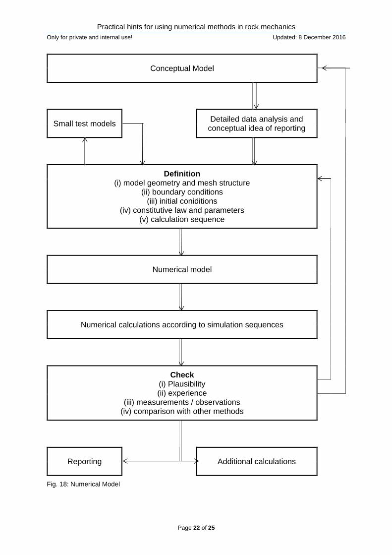
Phase 2: Numerical model:

In a second step the ‚Numerical Model‘ (Fig. 18) hast to be set-up, which means to perform the detailed programming including specification of initial and boundary con-ditions, meshing, parameter specification etc. The second phase starts with a detailed analysis of the data base and demands also thinking ahead, how and which model results should be obtained and documented. After that analysis, the model set-up starts with definition of the mesh, the initial and boundary conditions, the calculation sequence, the specification of constitutive laws und their parameters etc. in form of an input script or a menu-driven dialog. In case of any umbiguity / problem or to test the behavior, it is helpful to set up small models (in an extreme case a 1-zone-model) and to perform test simulations until the problem is exhausted. Then, the numerical simulation will be started and the model results will be stored for further evaluation. However, before reporting is started, the modelling results have to be checked carefully. Considering that, the following methods are available:

Plausibility check: that means to check, whether the calculated physical val-ues are generally feasible (are they within a plausible range? is the general deformation, stress and failure pattern logical?)

Comparison with experience: that means, are the model results located inside the field of experience and if not, can they be explained logical on a physical basis?

Direct comparison with measurements and / or observations in-situ. This ap-proach is always the best choice and should always be used.

Comparison with other calculation methods, either alternative numerical simu-lation approaches or semi-analytical solutions. This is already a demand at least for projects of special importance.

If the check of modelling results is positive, either the project can be finished by writ-ing a report or further simulations follow, e.g. in form of a parameter study, sensitivity analysis, robustness analysis, optimization, comparison between variants etc.

If the check of the modelling results is negative, one has to check if it is a more principal conceptual error (e.g. effect of water not considered, continuum approach not able to duplicate significant discontinuum effects etc.) or a more detailed error inside the nu-merical model (e.g. wrong parameter, wrong initial condition etc.) Depending on this evaluation one has to jump back inside the scheme, has to make corrections and then to execute all subsequent steps again. It is strongly recommended to perform geotechnical simulations always in parallel to the construction (project in-situ), that means starting already with the pre-planning phase until the phase of monitoring and backanalysis. Finally, this leads to more eco-nomic design, allows optimization and the chance to react short-termed to problematic situations, e.g. collapse. If such a strategy is applied, the numerical model will be step-by-step modified and improved (adjusted) according to the actual observations and measurement results. This, again, allows more and more precise predictions.



of 25

Conceptual Model

Small test models Detailed data analysis and

conceptual idea of reporting

Definition (i) model geometry and mesh structure

(ii) boundary conditions (iii) initial coniditions

(iv) constitutive law and parameters (v) calculation sequence

Numerical model

Numerical calculations according to simulation sequences

Check (i) Plausibility (ii) experience

(iii) measurements / observations (iv) comparison with other methods

Reporting

Additional calculations

Fig. 18: Numerical Model



of 25

13 Important terms

Verification (verify = make good)

Process to proof the correct mathematical-physical implementation of the desired al-gorithms / models etc. (in most cases done by comparison with analytical solutions or proofed numerical solutions – often called ‘Benchmarks’).

Validation (validate = become valid)

Process to determine, to what degree the underlying model represents reality in a cor-rect manner under chosen perspective (in most cases performed by comparison with observations and measurements in-situ or in the lab).

reality

conceptualmodel

numericalmodel

programmingsim

ula

tion

analysis

modellvalidation

modelverification

Fig.19: Role of verification and validation within the framework of simulation and software

development

Calibration:

Process of adjustment model parameters in such a way, that measured values are reproduced in a satisfying manner. The prerequisit is successful verification and vali-dation. Calibration can be achieved by trial-and-error procedure, by mathematical based backanalysis on the basis of special in-situ or labor tests or by mathematical based optimization.

Sensitivity analysis:

This analysis investigates the sensitivity of the model output as function of varying input parameters. This can be performed by a parameter study or in a more sophisticated and effective manner by stochastic sampling with statistical evaluation.

Parameter studies:

The model is run systematically with different parameter sets. The model response is evaluated as function of input parameters.

Uncertainty analysis:

Probabilistic modelling to determine the influence of fuzziness (range of variation) of input parameters on the model response.



of 25

Robustness analysis:

Probabilistic modelling to determine the robustness (stability) of the model response as function of varying (fluctuating) input values.

Reliability analysis:

This analysis investigates border violations (limit state violations) of the system behav-ior. The probability of failure is the quotient of number of model runs with failure to total number of model runs.

14 Current and future trends

There is an ongoing development of numerical simulation techniques. Some of the very active current research fields are listed below:

Multi-scale modelling High performance computing Automatic coupling of meshless and meshfree methods 3D-visualization within caves Integration of numerical models into GIS Coupling with optimization tools Integration of time-dependent and time-independent damage and fracture me-

chanical approaches into classical elasto-plastic ones Sophisticated HTMC-coupling

15 Literature

Batoz, J.-L. et al. (1980): A study of the three-node triangular plate bending elements, Int. J. Numerical Methods in Engineering, 15: 1771-1812 DGGT (2014): Empfehlungen des Arbeitskreises Numerik in der Geotechnik, Ernst & Sohn Groh, U. et al. (2011): Damage simulation of brittle heterogeneous materials at the grain size level,Theoretical and Applied Fracture Mechanics, 55: 31-38 Itasca (2011): FLAC Manuals, Itasca Consulting Group, Inc., Minneapolis, Minnesota, USA Itasca (2012): FLAC3D Manuals, Itasca Consulting Group, Inc., Minneapolis, Minne-sota, USA Jovanovic, M. et al. (2010): Accuracy of the FEM analysis in the function of the finite element type selection, Mechanical Engineering, 8(1): 1-8 Lisjak, A. & Grasselli, G. (2014). A review of discrete modelling techniques for fractur-ing processes in discontinuous rock mass, Int. J. Rock Mech. Min. Sci., 6: 301-314 Ljustina, G. et al. (2014): Rate sensitive continuum damage model sand mesh depend-ence in finite element analysis, The Scientific World Journal, ID 260571



of 25

Lunow, Ch. & Konietzky, H. (2009): Two dimensional simulation of the pressing and the cutting rock destruction., Proc. 2nd Int. Conf. on Computational Methods in Tun-neling, Aedificatio Publishers, 1: 223-230 Remacle, J.F. et al. (2010): Blossom-Quad: a non-uniform quadrilateral mesh genera-tor using a minimum cost perfect matching algorithm, Int. J. Num. Methods Engineer-ing, 00: 1-6 Sainsbury, D. et al. (2015): The use of Synthetic Rock Mass (SRM) modelling tech-niques to investigate joint rock mass strength and deformation behavior http://share.hydrofrac.wikispaces.net/file/view/Sainsbury_SRM.pdf (19.06.2015)

Stahl, M. & Konietzky, H., (2011): Discrete element simulation of ballast and gravel under special consideration of grain-shape, grain size and relative density, Granular Matter, 4: 417-428 Veyhl, C et al. (2010): On the mesh dependency of non-linear mechanical finite ele-ment analysis, Finite Elements in Analysis and Design, 46: 371-378 Wang, Z.L. & Konietzky, H., (2009): Modelling of blast-induced fractures in jointed rock mass, Engineering Fracture Mechanics, 76: 1945-1955.

http://share.hydrofrac.wikispaces.net/file/view/Sainsbury_SRM.pdf

Practical hints for using numerical methods in rock mechanics · Practical hints for using...

Documents

Transcript of Practical hints for using numerical methods in rock mechanics · Practical hints for using...