Practical Guide to Cluster Analysis in R · 2017-01-10 · Practical Guide To Cluster Analysis in R...
38
1 © A. Kassambara 2015 Multivariate Analysis I Alboukadel Kassambara Practical Guide To Cluster Analysis in R Edition 1 sthda.com Unsupervised Machine Learning
Transcript of Practical Guide to Cluster Analysis in R · 2017-01-10 · Practical Guide To Cluster Analysis in R...

1 © A. Kassambara 2015
Multivariate Analysis I
Alboukadel Kassambara
� Practical Guide To Cluster Analysis in R
Edition 1 sthda.com
Unsupervised Machine Learning

2
Copyright ©2017 by Alboukadel Kassambara. All rights reserved.
Published by STHDA (http://www.sthda.com), Alboukadel Kassambara
Contact: Alboukadel Kassambara <[email protected]>
No part of this publication may be reproduced, stored in a retrieval system, or transmitted in any formor by any means, electronic, mechanical, photocopying, recording, scanning, or otherwise, without the priorwritten permission of the Publisher. Requests to the Publisher for permission shouldbe addressed to STHDA (http://www.sthda.com).
Limit of Liability/Disclaimer of Warranty: While the publisher and author have used their best efforts inpreparing this book, they make no representations or warranties with respect to the accuracy orcompleteness of the contents of this book and specifically disclaim any implied warranties ofmerchantability or fitness for a particular purpose. No warranty may be created or extended by salesrepresentatives or written sales materials.
Neither the Publisher nor the authors, contributors, or editors,assume any liability for any injury and/or damageto persons or property as a matter of products liability,negligence or otherwise, or from any use or operation of anymethods, products, instructions, or ideas contained in the material herein.
For general information contact Alboukadel Kassambara <[email protected]>.

0.1. PREFACE 3
0.1 Preface
Large amounts of data are collected every day from satellite images, bio-medical,security, marketing, web search, geo-spatial or other automatic equipment. Miningknowledge from these big data far exceeds human’s abilities.
Clustering is one of the important data mining methods for discovering knowledgein multidimensional data. The goal of clustering is to identify pattern or groups ofsimilar objects within a data set of interest.
In the litterature, it is referred as “pattern recognition” or “unsupervised machinelearning” - “unsupervised” because we are not guided by a priori ideas of whichvariables or samples belong in which clusters. “Learning” because the machinealgorithm “learns” how to cluster.
Cluster analysis is popular in many fields, including:
• In cancer research for classifying patients into subgroups according their geneexpression profile. This can be useful for identifying the molecular profile ofpatients with good or bad prognostic, as well as for understanding the disease.
• In marketing for market segmentation by identifying subgroups of customers withsimilar profiles and who might be receptive to a particular form of advertising.
• In City-planning for identifying groups of houses according to their type, valueand location.
This book provides a practical guide to unsupervised machine learning or clusteranalysis using R software. Additionally, we developped an R package named factoextrato create, easily, a ggplot2-based elegant plots of cluster analysis results. Factoextraofficial online documentation: http://www.sthda.com/english/rpkgs/factoextra

4
0.2 About the author
Alboukadel Kassambara is a PhD in Bioinformatics and Cancer Biology. He works sincemany years on genomic data analysis and visualization. He created a bioinformaticstool named GenomicScape (www.genomicscape.com) which is an easy-to-use web toolfor gene expression data analysis and visualization.
He developed also a website called STHDA (Statistical Tools for High-throughput DataAnalysis, www.sthda.com/english), which contains many tutorials on data analysisand visualization using R software and packages.
He is the author of the R packages survminer (for analyzing and drawing survivalcurves), ggcorrplot (for drawing correlation matrix using ggplot2) and factoextra(to easily extract and visualize the results of multivariate analysis such PCA, CA,MCA and clustering). You can learn more about these packages at: http://www.sthda.com/english/wiki/r-packages
Recently, he published two books on data visualization:
1. Guide to Create Beautiful Graphics in R (at: https://goo.gl/vJ0OYb).2. Complete Guide to 3D Plots in R (at: https://goo.gl/v5gwl0).

Contents
0.1 Preface . . . . . . . . . . . . . . . . . . . . . . . . . . . . . . . . . . . 30.2 About the author . . . . . . . . . . . . . . . . . . . . . . . . . . . . . 40.3 Key features of this book . . . . . . . . . . . . . . . . . . . . . . . . . 90.4 How this book is organized? . . . . . . . . . . . . . . . . . . . . . . . 100.5 Book website . . . . . . . . . . . . . . . . . . . . . . . . . . . . . . . 160.6 Executing the R codes from the PDF . . . . . . . . . . . . . . . . . . 16
I Basics 17
1 Introduction to R 181.1 Install R and RStudio . . . . . . . . . . . . . . . . . . . . . . . . . . 181.2 Installing and loading R packages . . . . . . . . . . . . . . . . . . . . 191.3 Getting help with functions in R . . . . . . . . . . . . . . . . . . . . . 201.4 Importing your data into R . . . . . . . . . . . . . . . . . . . . . . . 201.5 Demo data sets . . . . . . . . . . . . . . . . . . . . . . . . . . . . . . 221.6 Close your R/RStudio session . . . . . . . . . . . . . . . . . . . . . . 22
2 Data Preparation and R Packages 232.1 Data preparation . . . . . . . . . . . . . . . . . . . . . . . . . . . . . 232.2 Required R Packages . . . . . . . . . . . . . . . . . . . . . . . . . . . 24
3 Clustering Distance Measures 253.1 Methods for measuring distances . . . . . . . . . . . . . . . . . . . . 253.2 What type of distance measures should we choose? . . . . . . . . . . 273.3 Data standardization . . . . . . . . . . . . . . . . . . . . . . . . . . . 283.4 Distance matrix computation . . . . . . . . . . . . . . . . . . . . . . 293.5 Visualizing distance matrices . . . . . . . . . . . . . . . . . . . . . . . 323.6 Summary . . . . . . . . . . . . . . . . . . . . . . . . . . . . . . . . . 33
5
6 CONTENTS
II Partitioning Clustering 34
4 K-Means Clustering 364.1 K-means basic ideas . . . . . . . . . . . . . . . . . . . . . . . . . . . 364.2 K-means algorithm . . . . . . . . . . . . . . . . . . . . . . . . . . . . 374.3 Computing k-means clustering in R . . . . . . . . . . . . . . . . . . . 384.4 K-means clustering advantages and disadvantages . . . . . . . . . . . 464.5 Alternative to k-means clustering . . . . . . . . . . . . . . . . . . . . 474.6 Summary . . . . . . . . . . . . . . . . . . . . . . . . . . . . . . . . . 47
5 K-Medoids 485.1 PAM concept . . . . . . . . . . . . . . . . . . . . . . . . . . . . . . . 495.2 PAM algorithm . . . . . . . . . . . . . . . . . . . . . . . . . . . . . . 495.3 Computing PAM in R . . . . . . . . . . . . . . . . . . . . . . . . . . 505.4 Summary . . . . . . . . . . . . . . . . . . . . . . . . . . . . . . . . . 56
6 CLARA - Clustering Large Applications 576.1 CLARA concept . . . . . . . . . . . . . . . . . . . . . . . . . . . . . 576.2 CLARA Algorithm . . . . . . . . . . . . . . . . . . . . . . . . . . . . 586.3 Computing CLARA in R . . . . . . . . . . . . . . . . . . . . . . . . . 586.4 Summary . . . . . . . . . . . . . . . . . . . . . . . . . . . . . . . . . 63
III Hierarchical Clustering 64
7 Agglomerative Clustering 677.1 Algorithm . . . . . . . . . . . . . . . . . . . . . . . . . . . . . . . . . 677.2 Steps to agglomerative hierarchical clustering . . . . . . . . . . . . . 687.3 Verify the cluster tree . . . . . . . . . . . . . . . . . . . . . . . . . . . 737.4 Cut the dendrogram into different groups . . . . . . . . . . . . . . . . 747.5 Cluster R package . . . . . . . . . . . . . . . . . . . . . . . . . . . . . 777.6 Application of hierarchical clustering to gene expression data analysis 777.7 Summary . . . . . . . . . . . . . . . . . . . . . . . . . . . . . . . . . 78
8 Comparing Dendrograms 798.1 Data preparation . . . . . . . . . . . . . . . . . . . . . . . . . . . . . 798.2 Comparing dendrograms . . . . . . . . . . . . . . . . . . . . . . . . . 80
9 Visualizing Dendrograms 849.1 Visualizing dendrograms . . . . . . . . . . . . . . . . . . . . . . . . . 859.2 Case of dendrogram with large data sets . . . . . . . . . . . . . . . . 90
CONTENTS 7
9.3 Manipulating dendrograms using dendextend . . . . . . . . . . . . . . 949.4 Summary . . . . . . . . . . . . . . . . . . . . . . . . . . . . . . . . . 96
10 Heatmap: Static and Interactive 9710.1 R Packages/functions for drawing heatmaps . . . . . . . . . . . . . . 9710.2 Data preparation . . . . . . . . . . . . . . . . . . . . . . . . . . . . . 9810.3 R base heatmap: heatmap() . . . . . . . . . . . . . . . . . . . . . . . 9810.4 Enhanced heat maps: heatmap.2() . . . . . . . . . . . . . . . . . . . 10110.5 Pretty heat maps: pheatmap() . . . . . . . . . . . . . . . . . . . . . . 10210.6 Interactive heat maps: d3heatmap() . . . . . . . . . . . . . . . . . . . 10310.7 Enhancing heatmaps using dendextend . . . . . . . . . . . . . . . . . 10310.8 Complex heatmap . . . . . . . . . . . . . . . . . . . . . . . . . . . . . 10410.9 Application to gene expression matrix . . . . . . . . . . . . . . . . . . 11410.10Summary . . . . . . . . . . . . . . . . . . . . . . . . . . . . . . . . . 116
IV Cluster Validation 117
11 Assessing Clustering Tendency 11911.1 Required R packages . . . . . . . . . . . . . . . . . . . . . . . . . . . 11911.2 Data preparation . . . . . . . . . . . . . . . . . . . . . . . . . . . . . 12011.3 Visual inspection of the data . . . . . . . . . . . . . . . . . . . . . . . 12011.4 Why assessing clustering tendency? . . . . . . . . . . . . . . . . . . . 12111.5 Methods for assessing clustering tendency . . . . . . . . . . . . . . . 12311.6 Summary . . . . . . . . . . . . . . . . . . . . . . . . . . . . . . . . . 127
12 Determining the Optimal Number of Clusters 12812.1 Elbow method . . . . . . . . . . . . . . . . . . . . . . . . . . . . . . . 12912.2 Average silhouette method . . . . . . . . . . . . . . . . . . . . . . . . 13012.3 Gap statistic method . . . . . . . . . . . . . . . . . . . . . . . . . . . 13012.4 Computing the number of clusters using R . . . . . . . . . . . . . . . 13112.5 Summary . . . . . . . . . . . . . . . . . . . . . . . . . . . . . . . . . 137
13 Cluster Validation Statistics 13813.1 Internal measures for cluster validation . . . . . . . . . . . . . . . . . 13913.2 External measures for clustering validation . . . . . . . . . . . . . . . 14113.3 Computing cluster validation statistics in R . . . . . . . . . . . . . . 14213.4 Summary . . . . . . . . . . . . . . . . . . . . . . . . . . . . . . . . . 150
14 Choosing the Best Clustering Algorithms 15114.1 Measures for comparing clustering algorithms . . . . . . . . . . . . . 151

8 CONTENTS
14.2 Compare clustering algorithms in R . . . . . . . . . . . . . . . . . . . 15214.3 Summary . . . . . . . . . . . . . . . . . . . . . . . . . . . . . . . . . 155
15 Computing P-value for Hierarchical Clustering 15615.1 Algorithm . . . . . . . . . . . . . . . . . . . . . . . . . . . . . . . . . 15615.2 Required packages . . . . . . . . . . . . . . . . . . . . . . . . . . . . 15715.3 Data preparation . . . . . . . . . . . . . . . . . . . . . . . . . . . . . 15715.4 Compute p-value for hierarchical clustering . . . . . . . . . . . . . . . 158
V Advanced Clustering 161
16 Hierarchical K-Means Clustering 16316.1 Algorithm . . . . . . . . . . . . . . . . . . . . . . . . . . . . . . . . . 16316.2 R code . . . . . . . . . . . . . . . . . . . . . . . . . . . . . . . . . . . 16416.3 Summary . . . . . . . . . . . . . . . . . . . . . . . . . . . . . . . . . 166
17 Fuzzy Clustering 16717.1 Required R packages . . . . . . . . . . . . . . . . . . . . . . . . . . . 16717.2 Computing fuzzy clustering . . . . . . . . . . . . . . . . . . . . . . . 16817.3 Summary . . . . . . . . . . . . . . . . . . . . . . . . . . . . . . . . . 170
18 Model-Based Clustering 17118.1 Concept of model-based clustering . . . . . . . . . . . . . . . . . . . . 17118.2 Estimating model parameters . . . . . . . . . . . . . . . . . . . . . . 17318.3 Choosing the best model . . . . . . . . . . . . . . . . . . . . . . . . . 17318.4 Computing model-based clustering in R . . . . . . . . . . . . . . . . . 17318.5 Visualizing model-based clustering . . . . . . . . . . . . . . . . . . . 175
19 DBSCAN: Density-Based Clustering 17719.1 Why DBSCAN? . . . . . . . . . . . . . . . . . . . . . . . . . . . . . . 17819.2 Algorithm . . . . . . . . . . . . . . . . . . . . . . . . . . . . . . . . . 18019.3 Advantages . . . . . . . . . . . . . . . . . . . . . . . . . . . . . . . . 18119.4 Parameter estimation . . . . . . . . . . . . . . . . . . . . . . . . . . . 18219.5 Computing DBSCAN . . . . . . . . . . . . . . . . . . . . . . . . . . . 18219.6 Method for determining the optimal eps value . . . . . . . . . . . . . 18419.7 Cluster predictions with DBSCAN algorithm . . . . . . . . . . . . . . 185
20 References and Further Reading 186
0.3. KEY FEATURES OF THIS BOOK 9
0.3 Key features of this book
Although there are several good books on unsupervised machine learning/clusteringand related topics, we felt that many of them are either too high-level, theoreticalor too advanced. Our goal was to write a practical guide to cluster analysis, elegantvisualization and interpretation.
The main parts of the book include:
• distance measures,• partitioning clustering,• hierarchical clustering,• cluster validation methods, as well as,• advanced clustering methods such as fuzzy clustering, density-based clustering
and model-based clustering.
The book presents the basic principles of these tasks and provide many examples inR. This book offers solid guidance in data mining for students and researchers.
Key features:
• Covers clustering algorithm and implementation• Key mathematical concepts are presented• Short, self-contained chapters with practical examples. This means that, you
don’t need to read the different chapters in sequence.
At the end of each chapter, we present R lab sections in which we systematicallywork through applications of the various methods discussed in that chapter.

10 CONTENTS
0.4 How this book is organized?
This book contains 5 parts. Part I (Chapter 1 - 3) provides a quick introduction toR (chapter 1) and presents required R packages and data format (Chapter 2) forclustering analysis and visualization.
The classification of objects, into clusters, requires some methods for measuring thedistance or the (dis)similarity between the objects. Chapter 3 covers the commondistance measures used for assessing similarity between observations.
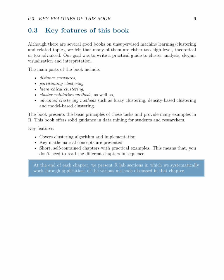
Part II starts with partitioning clustering methods, which include:
• K-means clustering (Chapter 4),• K-Medoids or PAM (partitioning around medoids) algorithm (Chapter 5) and• CLARA algorithms (Chapter 6).
Partitioning clustering approaches subdivide the data sets into a set of k groups, wherek is the number of groups pre-specified by the analyst.
0.4. HOW THIS BOOK IS ORGANIZED? 11
AlabamaAlaska
Arizona
Arkansas
CaliforniaColorado Connecticut
Delaware
Florida
Georgia
Hawaii
Idaho
Illinois
Indiana
IowaKansas
KentuckyLouisianaMaineMaryland
Massachusetts
Michigan
Minnesota
Mississippi
Missouri
Montana
Nebraska
Nevada
New Hampshire
New Jersey
New Mexico
New York
North Carolina
North Dakota
Ohio
Oklahoma
Oregon Pennsylvania
Rhode Island
South Carolina
South Dakota
Tennessee
Texas
Utah
Vermont
Virginia
Washington
West Virginia
Wisconsin
Wyoming
-1
0
1
2
-2 0 2Dim1 (62%)
Dim
2 (
24
.7%
)
cluster a a a a1 2 3 4
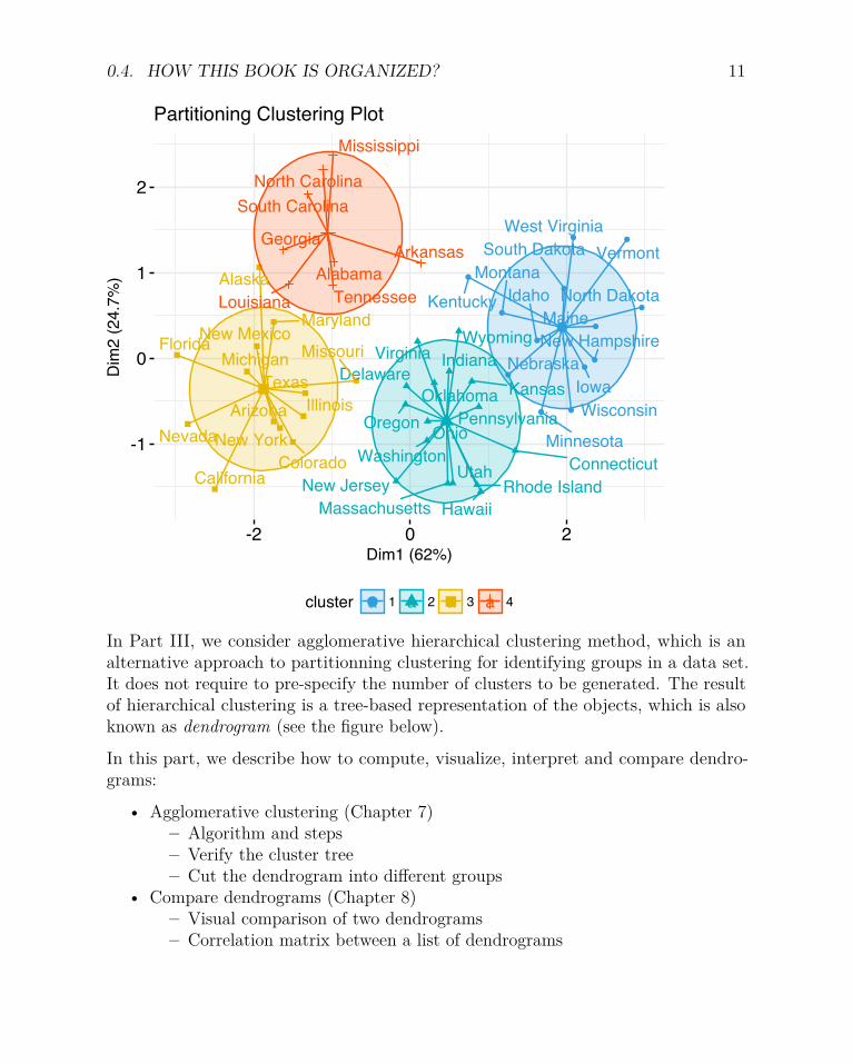
Partitioning Clustering Plot
In Part III, we consider agglomerative hierarchical clustering method, which is analternative approach to partitionning clustering for identifying groups in a data set.It does not require to pre-specify the number of clusters to be generated. The resultof hierarchical clustering is a tree-based representation of the objects, which is alsoknown as dendrogram (see the figure below).
In this part, we describe how to compute, visualize, interpret and compare dendro-grams:
• Agglomerative clustering (Chapter 7)– Algorithm and steps– Verify the cluster tree– Cut the dendrogram into different groups
• Compare dendrograms (Chapter 8)– Visual comparison of two dendrograms– Correlation matrix between a list of dendrograms

12 CONTENTS
• Visualize dendrograms (Chapter 9)– Case of small data sets– Case of dendrogram with large data sets: zoom, sub-tree, PDF– Customize dendrograms using dendextend
• Heatmap: static and interactive (Chapter 10)– R base heat maps– Pretty heat maps– Interactive heat maps– Complex heatmap– Real application: gene expression data
In this section, you will learn how to generate and interpret the following plots.
• Standard dendrogram with filled rectangle around clusters:
Ala
ba
ma
Lo
uis
ian
aG
eo
rgia
Te
nn
esse
eN
ort
h C
aro
lina
Mis
sis
sip
pi
So
uth
Ca
rolin
aT
exa
sIll
ino
isN
ew
Yo
rkF
lori
da
Ari
zo
na
Mic
hig
an
Ma
ryla
nd
Ne
w M
exic
oA
laska
Co
lora
do
Ca
lifo
rnia
Ne
va
da
So
uth
Da
kota
We
st V
irg
inia
No
rth
Da
kota
Ve
rmo
nt
Ida
ho
Mo
nta
na
Ne
bra
ska
Min
ne
so
taW
isco
nsin
Ma
ine
Iow
aN
ew
Ha
mpsh
ire
Vir
gin
iaW
yo
min
gA
rka
nsa
sK
en
tucky
De
law
are
Ma
ssa
ch
use
tts
Ne
w J
ers
ey
Co
nn
ectic
ut
Rh
od
e Isla
nd
Mis
so
uri
Ore
go
nW
ash
ing
ton
Okla
ho
ma
Ind
ian
aK
an
sa
sO
hio
Pe
nn
sylv
ania
Ha
wa
iiU
tah0
5
10
He
igh
t
Cluster Dendrogram

0.4. HOW THIS BOOK IS ORGANIZED? 13
• Compare two dendrograms:
3.0 2.0 1.0 0.0
Maine
Iowa
Wisconsin
Rhode Island
Utah
Mississippi
Maryland
Arizona
Tennessee
Virginia
0 1 2 3 4 5 6
Maryland
Arizona
Mississippi
Tennessee
Virginia
Maine
Iowa
Wisconsin
Rhode Island
Utah
• Heatmap:
carb
wt
hp cyl
disp
qsec
vs mpg
drat
am gear
Hornet 4 DriveValiantMerc 280Merc 280CToyota CoronaMerc 240DMerc 230Porsche 914−2Lotus EuropaDatsun 710Volvo 142EHonda CivicFiat X1−9Fiat 128Toyota CorollaChrysler ImperialCadillac FleetwoodLincoln ContinentalDuster 360Camaro Z28Merc 450SLCMerc 450SEMerc 450SLHornet SportaboutPontiac FirebirdDodge ChallengerAMC JavelinFerrari DinoMazda RX4Mazda RX4 WagFord Pantera LMaserati Bora
−1
0
1
2
3

14 CONTENTS
Part IV describes clustering validation and evaluation strategies, which consists ofmeasuring the goodness of clustering results. Before applying any clustering algorithmto a data set, the first thing to do is to assess the clustering tendency. That is,whether applying clustering is suitable for the data. If yes, then how many clustersare there. Next, you can perform hierarchical clustering or partitioning clustering(with a pre-specified number of clusters). Finally, you can use a number of measures,described in this chapter, to evaluate the goodness of the clustering results.
The different chapters included in part IV are organized as follow:
• Assessing clustering tendency (Chapter 11)
• Determining the optimal number of clusters (Chapter 12)
• Cluster validation statistics (Chapter 13)
• Choosing the best clustering algorithms (Chapter 14)
• Computing p-value for hierarchical clustering (Chapter 15)
In this section, you’ll learn how to create and interpret the plots hereafter.
• Visual assessment of clustering tendency (left panel): Clustering tendencyis detected in a visual form by counting the number of square shaped dark blocksalong the diagonal in the image.
• Determine the optimal number of clusters (right panel) in a data set usingthe gap statistics.
0
2
4
6
value
Clustering tendency
0.2
0.3
0.4
0.5
1 2 3 4 5 6 7 8 9 10Number of clusters k
Ga
p s
tatis
tic (
k)
Optimal number of clusters

0.4. HOW THIS BOOK IS ORGANIZED? 15
• Cluster validation using the silhouette coefficient (Si): A value of Si close to 1indicates that the object is well clustered. A value of Si close to -1 indicatesthat the object is poorly clustered. The figure below shows the silhouette plotof a k-means clustering.
0.00
0.25
0.50
0.75
1.00
Silh
ou
ett
e w
idth
Si
cluster 1 2 3
Clusters silhouette plot Average silhouette width: 0.46
Part V presents advanced clustering methods, including:
• Hierarchical k-means clustering (Chapter 16)• Fuzzy clustering (Chapter 17)• Model-based clustering (Chapter 18)• DBSCAN: Density-Based Clustering (Chapter 19)
The hierarchical k-means clustering is an hybrid approach for improving k-meansresults.
In Fuzzy clustering, items can be a member of more than one cluster. Each item has aset of membership coefficients corresponding to the degree of being in a given cluster.
In model-based clustering, the data are viewed as coming from a distribution that ismixture of two ore more clusters. It finds best fit of models to data and estimates thenumber of clusters.
The density-based clustering (DBSCAN is a partitioning method that has been intro-duced in Ester et al. (1996). It can find out clusters of different shapes and sizes fromdata containing noise and outliers.

16 CONTENTS
-3
-2
-1
0
1
-1 0 1x value
y v
alu
e
cluster 1 2 3 4 5
Density-based clustering
0.5 Book website
The website for this book is located at : http://www.sthda.com/english/. It containsnumber of ressources.
0.6 Executing the R codes from the PDF
For a single line R code, you can just copy the code from the PDF to the R console.
For a multiple-line R codes, an error is generated, sometimes, when you copy andpaste directly the R code from the PDF to the R console. If this happens, a solutionis to:
• Paste firstly the code in your R code editor or in your text editor• Copy the code from your text/code editor to the R console
Part I
Basics
17

Chapter 1
Introduction to R
R is a free and powerful statistical software for analyzing and visualizing data. Ifyou want to learn easily the essential of R programming, visit our series of tutorialsavailable on STHDA: http://www.sthda.com/english/wiki/r-basics-quick-and-easy.
In this chapter, we provide a very brief introduction to R, for installing R/RStudio aswell as importing your data into R.
1.1 Install R and RStudio
R and RStudio can be installed on Windows, MAC OSX and Linux platforms. RStudiois an integrated development environment for R that makes using R easier. It includesa console, code editor and tools for plotting.
1. R can be downloaded and installed from the Comprehensive R Archive Network(CRAN) webpage (http://cran.r-project.org/).
2. After installing R software, install also the RStudio software available at:http://www.rstudio.com/products/RStudio/.
3. Launch RStudio and start use R inside R studio.
18

1.2. INSTALLING AND LOADING R PACKAGES 19
RStudio screen:
1.2 Installing and loading R packages
An R package is an extension of R containing data sets and specific R functions tosolve specific questions.
For example, in this book, you’ll learn how to compute easily clustering algorithmusing the cluster R package.
There are thousands other R packages available for download and installation fromCRAN, Bioconductor(biology related R packages) and GitHub repositories.
1. How to install packages from CRAN? Use the function install.packages():
install.packages("cluster")
2. How to install packages from GitHub? You should first install devtools if youdon’t have it already installed on your computer:
For example, the following R code installs the latest version of factoextra R pack-age developed by A. Kassambara (https://github.com/kassambara/facoextra) formultivariate data analysis and elegant visualization..

20 CHAPTER 1. INTRODUCTION TO R
install.packages("devtools")devtools::install_github("kassambara/factoextra")
Note that, GitHub contains the developmental version of R packages.
3. After installation, you must first load the package for using the functions in thepackage. The function library() is used for this task.
library("cluster")
Now, we can use R functions in the cluster package for computing clustering algo-rithms, such as PAM (Partitioning Around Medoids).
1.3 Getting help with functions in R
If you want to learn more about a given function, say kmeans(), type this:
?kmeans
1.4 Importing your data into R
1. Prepare your file as follow:
• Use the first row as column names. Generally, columns represent variables• Use the first column as row names. Generally rows represent observations.• Each row/column name should be unique, so remove duplicated names.• Avoid names with blank spaces. Good column names: Long_jump or Long.jump.
Bad column name: Long jump.• Avoid names with special symbols: ?, $, *, +, #, (, ), -, /, }, {, |, >, < etc.
Only underscore can be used.• Avoid beginning variable names with a number. Use letter instead. Good column
names: sport_100m or x100m. Bad column name: 100m• R is case sensitive. This means that Name is different from Name or NAME.• Avoid blank rows in your data• Delete any comments in your file

1.4. IMPORTING YOUR DATA INTO R 21
• Replace missing values by NA (for not available)• If you have a column containing date, use the four digit format. Good format:
01/01/2016. Bad format: 01/01/16
2. Our final file should look like this:
3. Save your file
We recommend to save your file into .txt (tab-delimited text file) or .csv (commaseparated value file) format.
4. Get your data into R:
Use the R code below. You will be asked to choose a file:
# .txt file: Read tab separated valuesmy_data <- read.delim(file.choose())
# .csv file: Read comma (",") separated valuesmy_data <- read.csv(file.choose())
# .csv file: Read semicolon (";") separated valuesmy_data <- read.csv2(file.choose())
You can read more about how to import data into R at this link:http://www.sthda.com/english/wiki/importing-data-into-r
22 CHAPTER 1. INTRODUCTION TO R
1.5 Demo data sets
R comes with several built-in data sets, which are generally used as demo data forplaying with R functions. The most used R demo data sets include: USArrests, irisand mtcars. To load a demo data set, use the function data() as follow:
data("USArrests") # Loadinghead(USArrests, 3) # Print the first 3 rows
## Murder Assault UrbanPop Rape## Alabama 13.2 236 58 21.2## Alaska 10.0 263 48 44.5## Arizona 8.1 294 80 31.0
If you want learn more about USArrests data sets, type this:
?USArrests
USArrests data set is an object of class data frame.
To select just certain columns from a data frame, you can either refer to the columnsby name or by their location (i.e., column 1, 2, 3, etc.).
# Access the data in 'Murder' column# dollar sign is usedhead(USArrests$Murder)
## [1] 13.2 10.0 8.1 8.8 9.0 7.9
# Or use thisUSArrests[, 'Murder']
1.6 Close your R/RStudio session
Each time you close R/RStudio, you will be asked whether you want to save the datafrom your R session. If you decide to save, the data will be available in future Rsessions.

Chapter 2
Data Preparation and R Packages
2.1 Data preparation
To perform a cluster analysis in R, generally, the data should be prepared as follow:
1. Rows are observations (individuals) and columns are variables
2. Any missing value in the data must be removed or estimated.
3. The data must be standardized (i.e., scaled) to make variables comparable. Recallthat, standardization consists of transforming the variables such that they havemean zero and standard deviation one. Read more about data standardizationin chapter 3.
Here, we’ll use the built-in R data set “USArrests”, which contains statistics in arrestsper 100,000 residents for assault, murder, and rape in each of the 50 US states in 1973.It includes also the percent of the population living in urban areas.
data("USArrests") # Load the data setdf <- USArrests # Use df as shorter name
1. To remove any missing value that might be present in the data, type this:
df <- na.omit(df)
2. As we don’t want the clustering algorithm to depend to an arbitrary variableunit, we start by scaling/standardizing the data using the R function scale():
23

24 CHAPTER 2. DATA PREPARATION AND R PACKAGES
df <- scale(df)head(df, n = 3)
## Murder Assault UrbanPop Rape## Alabama 1.24256408 0.7828393 -0.5209066 -0.003416473## Alaska 0.50786248 1.1068225 -1.2117642 2.484202941## Arizona 0.07163341 1.4788032 0.9989801 1.042878388
2.2 Required R Packages
In this book, we’ll use mainly the following R packages:
• cluster for computing clustering algorithms, and• factoextra for ggplot2-based elegant visualization of clustering results. The
official online documentation is available at: http://www.sthda.com/english/rpkgs/factoextra.
factoextra contains many functions for cluster analysis and visualization, including:
Functions Descriptiondist(fviz_dist, get_dist) Distance Matrix Computation and Visualizationget_clust_tendency Assessing Clustering Tendencyfviz_nbclust(fviz_gap_stat) Determining the Optimal Number of Clustersfviz_dend Enhanced Visualization of Dendrogramfviz_cluster Visualize Clustering Resultsfviz_mclust Visualize Model-based Clustering Resultsfviz_silhouette Visualize Silhouette Information from Clusteringhcut Computes Hierarchical Clustering and Cut the Treehkmeans Hierarchical k-means clusteringeclust Visual enhancement of clustering analysis
To install the two packages, type this:
install.packages(c("cluster", "factoextra"))
Chapter 3
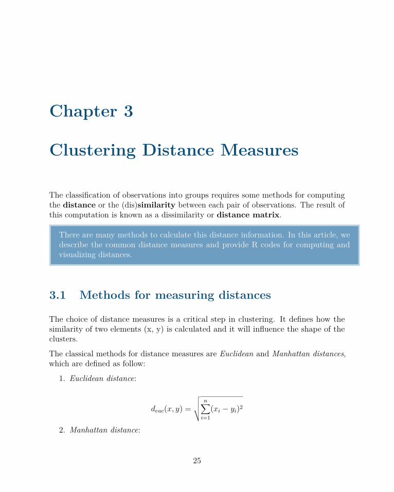
Clustering Distance Measures
The classification of observations into groups requires some methods for computingthe distance or the (dis)similarity between each pair of observations. The result ofthis computation is known as a dissimilarity or distance matrix.
There are many methods to calculate this distance information. In this article, wedescribe the common distance measures and provide R codes for computing andvisualizing distances.
3.1 Methods for measuring distances
The choice of distance measures is a critical step in clustering. It defines how thesimilarity of two elements (x, y) is calculated and it will influence the shape of theclusters.
The classical methods for distance measures are Euclidean and Manhattan distances,which are defined as follow:
1. Euclidean distance:
deuc(x, y) =√√√√ n∑i=1
(xi − yi)2
2. Manhattan distance:
25

26 CHAPTER 3. CLUSTERING DISTANCE MEASURES
dman(x, y) =n∑i=1|(xi − yi)|
Where, x and y are two vectors of length n.
Other dissimilarity measures exist such as correlation-based distances, which iswidely used for gene expression data analyses. Correlation-based distance is defined bysubtracting the correlation coefficient from 1. Different types of correlation methodscan be used such as:
1. Pearson correlation distance:
dcor(x, y) = 1−
n∑i=1
(xi − x)(yi − y)√n∑i=1
(xi − x)2n∑i=1
(yi − y)2
Pearson correlation measures the degree of a linear relationship between two profiles.
2. Eisen cosine correlation distance (Eisen et al., 1998):
It’s a special case of Pearson’s correlation with x and y both replaced by zero:
deisen(x, y) = 1−
∣∣∣∣ n∑i=1
xiyi
∣∣∣∣√n∑i=1
x2i
n∑i=1
y2i
3. Spearman correlation distance:
The spearman correlation method computes the correlation between the rank of x andthe rank of y variables.
dspear(x, y) = 1−
n∑i=1
(x′i − x′)(y′i − y′)√n∑i=1
(x′i − x′)2n∑i=1
(y′i − y′)2
Where x′i = rank(xi) and y′i = rank(y).

3.2. WHAT TYPE OF DISTANCE MEASURES SHOULD WE CHOOSE? 27
4. Kendall correlation distance:
Kendall correlation method measures the correspondence between the ranking of xand y variables. The total number of possible pairings of x with y observations isn(n− 1)/2, where n is the size of x and y. Begin by ordering the pairs by the x values.If x and y are correlated, then they would have the same relative rank orders. Now,for each yi, count the number of yj > yi (concordant pairs (c)) and the number ofyj < yi (discordant pairs (d)).
Kendall correlation distance is defined as follow:
dkend(x, y) = 1− nc − nd12n(n− 1)
Where,
• nc: total number of concordant pairs• nd: total number of discordant pairs• n: size of x and y
Note that,
- Pearson correlation analysis is the most commonly used method. It isalso known as a parametric correlation which depends on the distribution of thedata.- Kendall and Spearman correlations are non-parametric and they are used toperform rank-based correlation analysis.
In the formula above, x and y are two vectors of length n and, means x and y,respectively. The distance between x and y is denoted d(x, y).
3.2 What type of distance measures should wechoose?
The choice of distance measures is very important, as it has a strong influence on theclustering results. For most common clustering software, the default distance measureis the Euclidean distance.

28 CHAPTER 3. CLUSTERING DISTANCE MEASURES
Depending on the type of the data and the researcher questions, other dissimilaritymeasures might be preferred. For example, correlation-based distance is often used ingene expression data analysis.
Correlation-based distance considers two objects to be similar if their features arehighly correlated, even though the observed values may be far apart in terms ofEuclidean distance. The distance between two objects is 0 when they are perfectlycorrelated. Pearson’s correlation is quite sensitive to outliers. This does not matterwhen clustering samples, because the correlation is over thousands of genes. Whenclustering genes, it is important to be aware of the possible impact of outliers. Thiscan be mitigated by using Spearman’s correlation instead of Pearson’s correlation.
If we want to identify clusters of observations with the same overall profiles regardlessof their magnitudes, then we should go with correlation-based distance as a dissimilaritymeasure. This is particularly the case in gene expression data analysis, where wemight want to consider genes similar when they are “up” and “down” together. It isalso the case, in marketing if we want to identify group of shoppers with the samepreference in term of items, regardless of the volume of items they bought.
If Euclidean distance is chosen, then observations with high values of features will beclustered together. The same holds true for observations with low values of features.
3.3 Data standardization
The value of distance measures is intimately related to the scale on which measurementsare made. Therefore, variables are often scaled (i.e. standardized) before measuring theinter-observation dissimilarities. This is particularly recommended when variables aremeasured in different scales (e.g: kilograms, kilometers, centimeters, . . . ); otherwise,the dissimilarity measures obtained will be severely affected.
The goal is to make the variables comparable. Generally variables are scaled to havei) standard deviation one and ii) mean zero.
The standardization of data is an approach widely used in the context of gene expressiondata analysis before clustering. We might also want to scale the data when the meanand/or the standard deviation of variables are largely different.
When scaling variables, the data can be transformed as follow:
xi − center(x)scale(x)

3.4. DISTANCE MATRIX COMPUTATION 29
Where center(x) can be the mean or the median of x values, and scale(x) can bethe standard deviation (SD), the interquartile range, or the MAD (median absolutedeviation).
The R base function scale() can be used to standardize the data. It takes a numericmatrix as an input and performs the scaling on the columns.
Standardization makes the four distance measure methods - Euclidean, Manhattan,Correlation and Eisen - more similar than they would be with non-transformed data.
Note that, when the data are standardized, there is a functional relation-ship between the Pearson correlation coefficient r(x, y) and the Euclidean distance.
With some maths, the relationship can be defined as follow:
deuc(x, y) =√
2m[1− r(x, y)]
Where x and y are two standardized m-vectors with zero mean and unit length.
Therefore, the result obtained with Pearson correlation measures and stan-dardized Euclidean distances are comparable.
3.4 Distance matrix computation
3.4.1 Data preparation
We’ll use the USArrests data as demo data sets. We’ll use only a subset of the databy taking 15 random rows among the 50 rows in the data set. This is done by usingthe function sample(). Next, we standardize the data using the function scale():
# Subset of the dataset.seed(123)ss <- sample(1:50, 15) # Take 15 random rowsdf <- USArrests[ss, ] # Subset the 15 rowsdf.scaled <- scale(df) # Standardize the variables

30 CHAPTER 3. CLUSTERING DISTANCE MEASURES
3.4.2 R functions and packages
There are many R functions for computing distances between pairs of observations:
1. dist() R base function [stats package]: Accepts only numeric data as an input.
2. get_dist() function [factoextra package]: Accepts only numeric data as an input.Compared to the standard dist() function, it supports correlation-based distancemeasures including “pearson”, “kendall” and “spearman” methods.
3. daisy() function [cluster package]: Able to handle other variable types (e.g. nom-inal, ordinal, (a)symmetric binary). In that case, the Gower’s coefficient willbe automatically used as the metric. It’s one of the most popular measures ofproximity for mixed data types. For more details, read the R documentation ofthe daisy() function (?daisy).
All these functions compute distances between rows of the data.
3.4.3 Computing euclidean distance
To compute Euclidean distance, you can use the R base dist() function, as follow:
dist.eucl <- dist(df.scaled, method = "euclidean")
Note that, allowed values for the option method include one of: “euclidean”, “maxi-mum”, “manhattan”, “canberra”, “binary”, “minkowski”.
To make it easier to see the distance information generated by the dist() function, youcan reformat the distance vector into a matrix using the as.matrix() function.
# Reformat as a matrix# Subset the first 3 columns and rows and Round the valuesround(as.matrix(dist.eucl)[1:3, 1:3], 1)
## Iowa Rhode Island Maryland## Iowa 0.0 2.8 4.1## Rhode Island 2.8 0.0 3.6## Maryland 4.1 3.6 0.0

3.4. DISTANCE MATRIX COMPUTATION 31
In this matrix, the value represent the distance between objects. The values on thediagonal of the matrix represent the distance between objects and themselves (whichare zero).
In this data set, the columns are variables. Hence, if we want to compute pairwisedistances between variables, we must start by transposing the data to have variablesin the rows of the data set before using the dist() function. The function t() is usedfor transposing the data.
3.4.4 Computing correlation based distances
Correlation-based distances are commonly used in gene expression data analysis.
The function get_dist()[factoextra package] can be used to compute correlation-baseddistances. Correlation method can be either pearson, spearman or kendall.
# Computelibrary("factoextra")dist.cor <- get_dist(df.scaled, method = "pearson")
# Display a subsetround(as.matrix(dist.cor)[1:3, 1:3], 1)
## Iowa Rhode Island Maryland## Iowa 0.0 0.4 1.9## Rhode Island 0.4 0.0 1.5## Maryland 1.9 1.5 0.0
3.4.5 Computing distances for mixed data
The function daisy() [cluster package] provides a solution (Gower’s metric) for com-puting the distance matrix, in the situation where the data contain no-numericcolumns.
The R code below applies the daisy() function on flower data which contains factor,ordered and numeric variables:

32 CHAPTER 3. CLUSTERING DISTANCE MEASURES
library(cluster)# Load datadata(flower)head(flower, 3)
## V1 V2 V3 V4 V5 V6 V7 V8## 1 0 1 1 4 3 15 25 15## 2 1 0 0 2 1 3 150 50## 3 0 1 0 3 3 1 150 50
# Data structurestr(flower)
## 'data.frame': 18 obs. of 8 variables:## $ V1: Factor w/ 2 levels "0","1": 1 2 1 1 1 1 1 1 2 2 ...## $ V2: Factor w/ 2 levels "0","1": 2 1 2 1 2 2 1 1 2 2 ...## $ V3: Factor w/ 2 levels "0","1": 2 1 1 2 1 1 1 2 1 1 ...## $ V4: Factor w/ 5 levels "1","2","3","4",..: 4 2 3 4 5 4 4 2 3 5 ...## $ V5: Ord.factor w/ 3 levels "1"<"2"<"3": 3 1 3 2 2 3 3 2 1 2 ...## $ V6: Ord.factor w/ 18 levels "1"<"2"<"3"<"4"<..: 15 3 1 16 2 12 13 7 4 14 ...## $ V7: num 25 150 150 125 20 50 40 100 25 100 ...## $ V8: num 15 50 50 50 15 40 20 15 15 60 ...
# Distance matrixdd <- daisy(flower)round(as.matrix(dd)[1:3, 1:3], 2)
## 1 2 3## 1 0.00 0.89 0.53## 2 0.89 0.00 0.51## 3 0.53 0.51 0.00
3.5 Visualizing distance matrices
A simple solution for visualizing the distance matrices is to use the function fviz_dist()[factoextra package]. Other specialized methods, such as agglomerative hierarchicalclustering (Chapter 7) or heatmap (Chapter 10) will be comprehensively described in
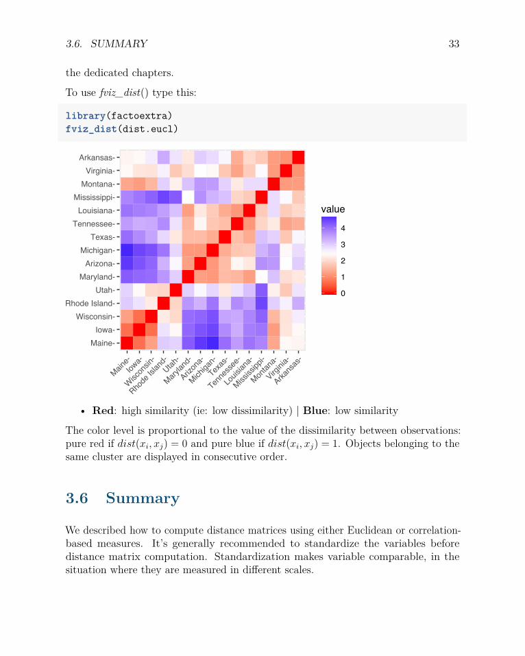
3.6. SUMMARY 33
the dedicated chapters.
To use fviz_dist() type this:
library(factoextra)fviz_dist(dist.eucl)
Maine-
Iowa-
Wisconsin-
Rhode Island-
Utah-
Maryland-
Arizona-
Michigan-
Texas-
Tennessee-
Louisiana-
Mississippi-
Montana-
Virginia-
Arkansas-
Maine
-
Iowa-
Wisco
nsin-
Rho
de Is
land
-
Uta
h-
Mar
ylan
d-
Arizon
a-
Michiga
n-
Texas
-
Tenne
ssee
-
Louisian
a-
Mississ
ippi-
Mon
tana
-
Virginia-
Arkan
sas-
0
1
2
3
4
value
• Red: high similarity (ie: low dissimilarity) | Blue: low similarity
The color level is proportional to the value of the dissimilarity between observations:pure red if dist(xi, xj) = 0 and pure blue if dist(xi, xj) = 1. Objects belonging to thesame cluster are displayed in consecutive order.
3.6 Summary
We described how to compute distance matrices using either Euclidean or correlation-based measures. It’s generally recommended to standardize the variables beforedistance matrix computation. Standardization makes variable comparable, in thesituation where they are measured in different scales.
Part II
Partitioning Clustering
34

35
Partitioning clustering are clustering methods used to classify observations, withina data set, into multiple groups based on their similarity. The algorithms require theanalyst to specify the number of clusters to be generated.
This chapter describes the commonly used partitioning clustering, including:
• K-means clustering (MacQueen, 1967), in which, each cluster is representedby the center or means of the data points belonging to the cluster. The K-meansmethod is sensitive to anomalous data points and outliers.
• K-medoids clustering or PAM (Partitioning Around Medoids, Kaufman &Rousseeuw, 1990), in which, each cluster is represented by one of the objects inthe cluster. PAM is less sensitive to outliers compared to k-means.
• CLARA algorithm (Clustering Large Applications), which is an extension toPAM adapted for large data sets.
For each of these methods, we provide:
• the basic idea and the key mathematical concepts• the clustering algorithm and implementation in R software• R lab sections with many examples for cluster analysis and visualization
The following R packages will be used to compute and visualize partitioning clustering:
• stats package for computing K-means• cluster package for computing PAM and CLARA algorithms• factoextra for beautiful visualization of clusters

Chapter 4
K-Means Clustering
K-means clustering (MacQueen, 1967) is the most commonly used unsupervisedmachine learning algorithm for partitioning a given data set into a set of k groups (i.e.k clusters), where k represents the number of groups pre-specified by the analyst. Itclassifies objects in multiple groups (i.e., clusters), such that objects within the samecluster are as similar as possible (i.e., high intra-class similarity), whereas objectsfrom different clusters are as dissimilar as possible (i.e., low inter-class similarity).In k-means clustering, each cluster is represented by its center (i.e, centroid) whichcorresponds to the mean of points assigned to the cluster.
In this article, we’ll describe the k-means algorithm and provide practical examplesusing R software.
4.1 K-means basic ideas
The basic idea behind k-means clustering consists of defining clusters so that the totalintra-cluster variation (known as total within-cluster variation) is minimized.
There are several k-means algorithms available. The standard algorithm is theHartigan-Wong algorithm (1979), which defines the total within-cluster variation asthe sum of squared distances Euclidean distances between items and the correspondingcentroid:
36

4.2. K-MEANS ALGORITHM 37
W (Ck) =∑xi∈Ck
(xi − µk)2
• xi design a data point belonging to the cluster Ck• µk is the mean value of the points assigned to the cluster Ck
Each observation (xi) is assigned to a given cluster such that the sum of squares (SS)distance of the observation to their assigned cluster centers µk is a minimum.
We define the total within-cluster variation as follow:
tot.withinss =k∑k=1
W (Ck) =k∑k=1
∑xi∈Ck
(xi − µk)2
The total within-cluster sum of square measures the compactness (i.e goodness) of theclustering and we want it to be as small as possible.
4.2 K-means algorithm
The first step when using k-means clustering is to indicate the number of clusters (k)that will be generated in the final solution.
The algorithm starts by randomly selecting k objects from the data set to serve as theinitial centers for the clusters. The selected objects are also known as cluster meansor centroids.
Next, each of the remaining objects is assigned to it’s closest centroid, where closest isdefined using the Euclidean distance (Chapter 3) between the object and the clustermean. This step is called “cluster assignment step”. Note that, to use correlationdistance, the data are input as z-scores.
After the assignment step, the algorithm computes the new mean value of each cluster.The term cluster “centroid update” is used to design this step. Now that the centershave been recalculated, every observation is checked again to see if it might be closerto a different cluster. All the objects are reassigned again using the updated clustermeans.
The cluster assignment and centroid update steps are iteratively repeated until thecluster assignments stop changing (i.e until convergence is achieved). That is, the

38 CHAPTER 4. K-MEANS CLUSTERING
clusters formed in the current iteration are the same as those obtained in the previousiteration.
K-means algorithm can be summarized as follow:
1. Specify the number of clusters (K) to be created (by the analyst)
2. Select randomly k objects from the data set as the initial cluster centers or means
3. Assigns each observation to their closest centroid, based on the Euclideandistance between the object and the centroid
4. For each of the k clusters update the cluster centroid by calculating the newmean values of all the data points in the cluster. The centoid of a Kth clusteris a vector of length p containing the means of all variables for the observationsin the kth cluster; p is the number of variables.
5. Iteratively minimize the total within sum of square. That is, iterate steps 3and 4 until the cluster assignments stop changing or the maximum number ofiterations is reached. By default, the R software uses 10 as the default valuefor the maximum number of iterations.
4.3 Computing k-means clustering in R
4.3.1 Data
We’ll use the demo data sets “USArrests”. The data should be prepared as describedin chapter 2. The data must contains only continuous variables, as the k-meansalgorithm uses variable means. As we don’t want the k-means algorithm to depend toan arbitrary variable unit, we start by scaling the data using the R function scale() asfollow:
data("USArrests") # Loading the data setdf <- scale(USArrests) # Scaling the data
# View the firt 3 rows of the datahead(df, n = 3)