Practical ERM
34
1 Practical ERM Midwestern Actuarial Forum Fall 2005 Meeting Chris Suchar, FCAS
-
Upload
barbara-beasley -
Category
Documents
-
view
161 -
download
14
description
Practical ERM. Midwestern Actuarial Forum Fall 2005 Meeting Chris Suchar, FCAS. Discussion Outline. Background on Implementation Examples of Real World Issues and Uses Financial Planning Capital Management Reinsurance Analysis Investment – Asset allocation and Risk/Return Analysis - PowerPoint PPT Presentation
Transcript of Practical ERM
1
Practical ERM
Midwestern Actuarial Forum
Fall 2005 Meeting
Chris Suchar, FCAS
2
Discussion Outline
• Background on Implementation
• Examples of Real World Issues and Uses
– Financial Planning
– Capital Management
– Reinsurance Analysis
– Investment – Asset allocation and Risk/Return Analysis
– Analysis of Incentive Compensation Goals
– Accounting / Reporting Issue – Fin. 46
3
Background Information
• Tool used “Advise” from DFA Capital Management
• Purchased, installed, trained, constructed data and created baseline model during 2003.
• Operational in six months. Keys to success were:
– Obtained executive sponsorship
– Managed project scope
– Proper dedicated resources
– Hard date on deliverables – Deliver Financial Model by Dec. 2003
• 2004 and 2005 years of continued enhancements
– More acceptance and understanding in quantifying the risk. – More appreciation of value added to the decision making process
4
Example of Financial / Operational Planning
5
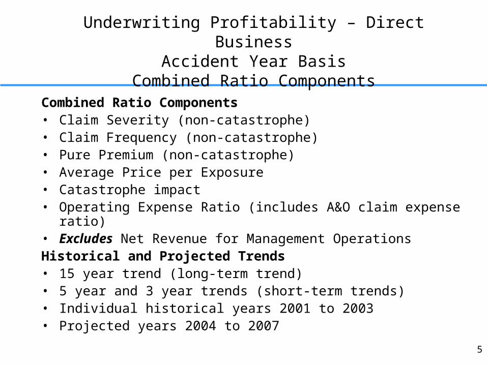
Underwriting Profitability – Direct BusinessAccident Year Basis
Combined Ratio Components
Combined Ratio Components • Claim Severity (non-catastrophe) • Claim Frequency (non-catastrophe) • Pure Premium (non-catastrophe)• Average Price per Exposure• Catastrophe impact• Operating Expense Ratio (includes A&O claim expense ratio)• Excludes Net Revenue for Management OperationsHistorical and Projected Trends • 15 year trend (long-term trend)• 5 year and 3 year trends (short-term trends)• Individual historical years 2001 to 2003• Projected years 2004 to 2007
6
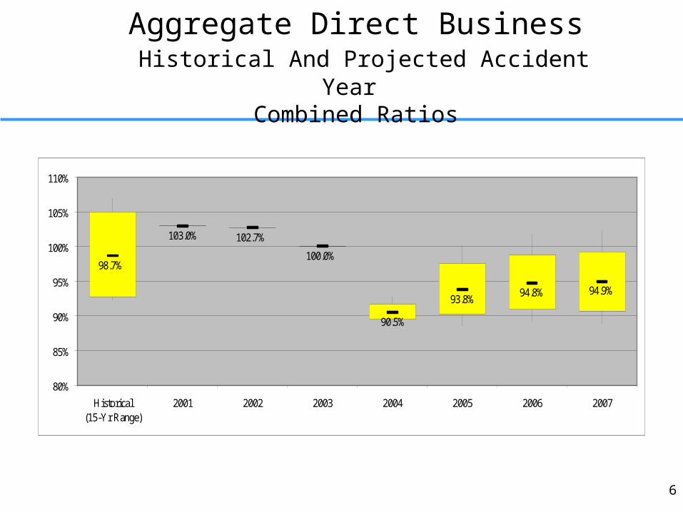
Aggregate Direct Business Historical And Projected Accident Year
Combined Ratios
98.7%
103.0% 102.7%
100.0%
90.5%
93.8%94.8% 94.9%
80%
85%
90%
95%
100%
105%
110%
Historical(15-Yr Range)
2001 2002 2003 2004 2005 2006 2007
7
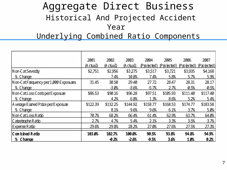
Aggregate Direct Business Historical And Projected Accident Year
Underlying Combined Ratio Components
2001(Actual)
2002(Actual)
2003(Actual)
2004(Projected)
2005(Projected)
2006(Projected)
2007(Projected)
Non-Cat Severity $2,751 $2,956 $3,275 $3,517 $3,721 $3,935 $4,168 % Change 7.4% 10.8% 7.4% 5.8% 5.7% 5.9%Non-Cat Frequency per 1,000 Exposures 31.45 30.50 29.40 27.72 28.47 28.31 28.17 % Change -3.0% -3.6% -5.7% 2.7% -0.5% -0.5%Non-Cat Loss Costs per Exposure $86.53 $90.16 $96.28 $97.51 $105.93 $111.40 $117.40 % Change 4.2% 6.8% 1.3% 8.6% 5.2% 5.4%Average Earned Price per Exposure $122.39 $132.25 $144.92 $158.77 $168.53 $174.77 $183.58 % Change 8.1% 9.6% 9.6% 6.1% 3.7% 5.0%Non-Cat Loss Ratio 70.7% 68.2% 66.4% 61.4% 62.9% 63.7% 64.0%Catastrophe Ratio 2.7% 4.7% 5.4% 2.1% 3.3% 3.5% 3.7%Expense Ratio 29.6% 29.8% 28.2% 27.0% 27.6% 27.5% 27.3%
Combined Ratio 103.0% 102.7% 100.0% 90.5% 93.8% 94.8% 94.9% % Change -0.3% -2.6% -9.5% 3.6% 1.0% 0.2%
8
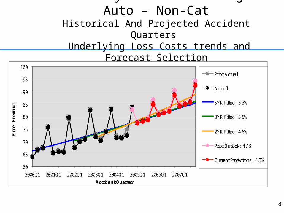
Voluntary Private Passenger Auto – Non-CatHistorical And Projected Accident Quarters
Underlying Loss Costs trends and Forecast Selection
60
65
70
75
80
85
90
95
100
2000Q1 2001Q1 2002Q1 2003Q1 2004Q1 2005Q1 2006Q1 2007Q1
Accident Quarter
Pure
Pre
miu
m
Prior Actual
Actual
5YR Fitted: 3.3%
3YR Fitted: 3.5%
2YR Fitted: 4.6%
Prior Outlook: 4.4%
Current Projections: 4.3%
9
Examples of Capital Management Issue
Capital Adequacy
Capital Efficiency
Stress Testing Capital
10
Stochastic Analysis Combined Property and Casualty Insurance Operations
• Capital Adequacy– Capital Adequacy = having enough capital, identifying the excess
• How much capital do we require?
• What is our tolerance for falling below our required capital level?
• Given an appropriate probability of falling below our required capital level, is there an excess or deficit of capital?
11
Capital Adequacy (Cont’d)
Combined Property and Casualty Insurance Operations
• How much capital do we require?
– Maintain A+ Benchmark Capital Levels• Equal to 2 times the NAIC Company Action Risk Based Capital
Level • Qualifies for an A++/A+ superior rating from A.M. Best
– NAIC Company Action Risk Based Capital Level• At beginning of simulation = $851 million• Assumed at end of simulation = $1.035 billion
– A+ Benchmark Capital Level• At beginning of simulation = $1.702 billion• Assumed at end of simulation = $2.072 billion
12
Capital Adequacy (Cont’d)
Combined Property and Casualty Insurance Operations
• What is our tolerance for falling below our required A+ Benchmark Capital Level?
– Simulation Assumption – 1 in 400 year event = 12,000 paths 99.5% overall certainty 99.75% certainty of downside Time Horizon – 2½ years
– Current catastrophe reinsurance agreement in force
– Includes variability of underwriting and investment risks
13
Capital Adequacy Combined Property and Casualty Insurance Operations
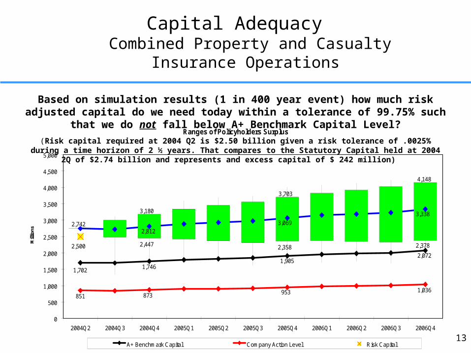
Based on simulation results (1 in 400 year event) how much risk adjusted capital do we need today within a tolerance of 99.75% such that we do not fall below A+ Benchmark Capital Level?
Ranges of Policyholders Surplus
3,180
3,703
4,148
2,742 3,069
3,338
2,812
2,3782,3582,447
1,9052,072
1,7461,702
1,036953873851
2,500
0
500
1,000
1,500
2,000
2,500
3,000
3,500
4,000
4,500
5,000
2004Q2 2004Q3 2004Q4 2005Q1 2005Q2 2005Q3 2005Q4 2006Q1 2006Q2 2006Q3 2006Q4
Mill
ions
A+ Benchmark Capital Company Action Level Risk Capital
(Risk capital required at 2004 Q2 is $2.50 billion given a risk tolerance of .0025% during a time horizon of 2 ½ years. That compares to the Statutory Capital held at 2004 2Q of $2.74 billion and represents and excess capital of $ 242 million)
14
Capital Adequacy (Cont’d)
Combined Property and Casualty Insurance Operations
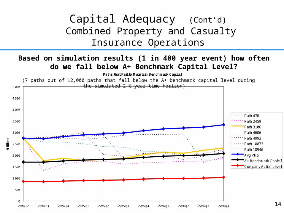
Based on simulation results (1 in 400 year event) how often do we fall below A+ Benchmark Capital Level?Paths that Fail to Maintain Benchmark Capital
0
500
1,000
1,500
2,000
2,500
3,000
3,500
4,000
4,500
5,000
2004Q2 2004Q3 2004Q4 2005Q1 2005Q2 2005Q3 2005Q4 2006Q1 2006Q2 2006Q3 2006Q4
Mill
ion
s
Path 470
Path 2459
Path 3106
Path 4606
Path 4992
Path 10873
Path 10946
Avg PHS
A+ Benchmark Capital
Company Action Level
(7 paths out of 12,000 paths that fall below the A+ benchmark capital level during the simulated 2 ½ year time horizon)
15
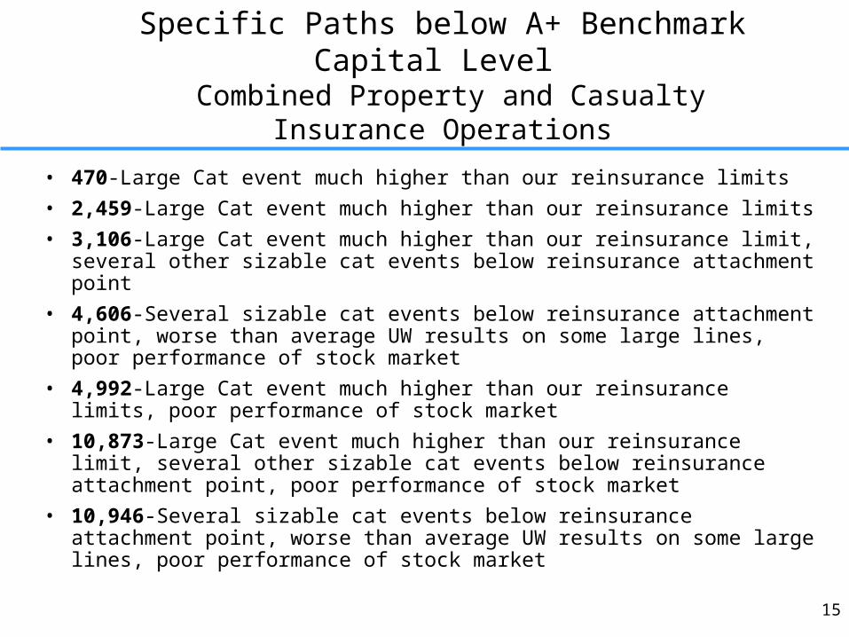
Specific Paths below A+ Benchmark Capital Level Combined Property and Casualty Insurance Operations
• 470-Large Cat event much higher than our reinsurance limits
• 2,459-Large Cat event much higher than our reinsurance limits
• 3,106-Large Cat event much higher than our reinsurance limit, several other sizable cat events below reinsurance attachment point
• 4,606-Several sizable cat events below reinsurance attachment point, worse than average UW results on some large lines, poor performance of stock market
• 4,992-Large Cat event much higher than our reinsurance limits, poor performance of stock market
• 10,873-Large Cat event much higher than our reinsurance limit, several other sizable cat events below reinsurance attachment point, poor performance of stock market
• 10,946-Several sizable cat events below reinsurance attachment point, worse than average UW results on some large lines, poor performance of stock market
16
Stochastic Analysis Combined Property and Casualty Insurance Operations
• Capital Efficiency– Capital Efficiency = producing an acceptable return on the capital
we hold
– How do we measure capital efficiency?• ROE = expected return / capital held
• EVA = expected return (hurdle rate x capital held)
– Identify • Economic vs. Statutory capital and surplus
• Annualized Average Return on Surplus – Economic basis: simulation period of two and half years ended December 31, 2006
• Risk adjusted value added
17
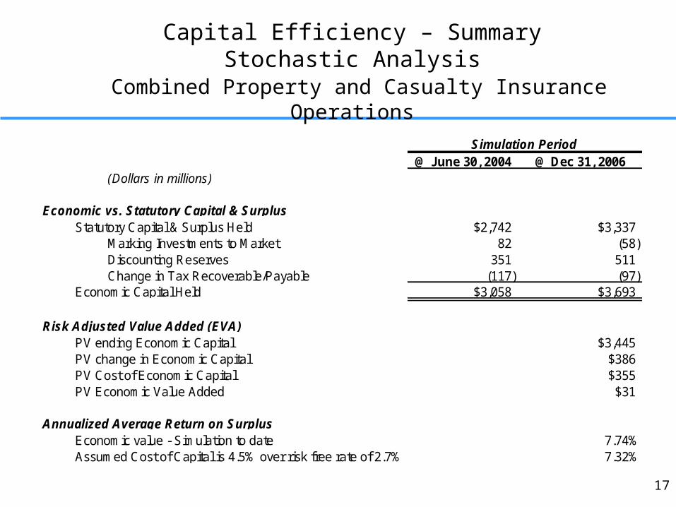
Capital Efficiency – Summary Stochastic Analysis
Combined Property and Casualty Insurance Operations
Simulation Period@ June 30, 2004 @ Dec 31, 2006
(Dollars in millions)
Economic vs. Statutory Capital & SurplusStatutory Capital & Surplus Held $2,742 $3,337
Marking Investments to Market 82 (58)Discounting Reserves 351 511Change in Tax Recoverable/Payable (117) (97)
Economic Capital Held $3,058 $3,693
Risk Adjusted Value Added (EVA)PV ending Economic Capital $3,445PV change in Economic Capital $386PV Cost of Economic Capital $355PV Economic Value Added $31
Annualized Average Return on Surplus Economic value - Simulation to date 7.74%Assumed Cost of Capital is 4.5% over risk free rate of 2.7% 7.32%
18
Stress Test AnalysisPolicyholders Surplus without Catastrophe Reinsurance
Combined Property and Casualty Insurance Operations
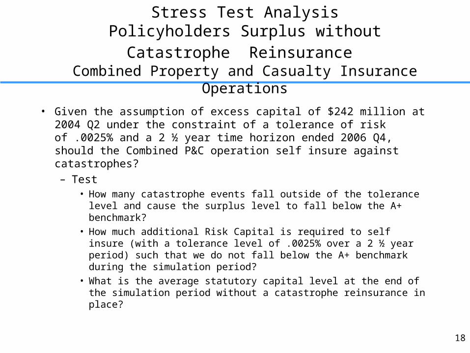
• Given the assumption of excess capital of $242 million at 2004 Q2 under the constraint of a tolerance of risk of .0025% and a 2 ½ year time horizon ended 2006 Q4, should the Combined P&C operation self insure against catastrophes?
– Test• How many catastrophe events fall outside of the tolerance level and
cause the surplus level to fall below the A+ benchmark?
• How much additional Risk Capital is required to self insure (with a tolerance level of .0025% over a 2 ½ year period) such that we do not fall below the A+ benchmark during the simulation period?
• What is the average statutory capital level at the end of the simulation period without a catastrophe reinsurance in place?
19
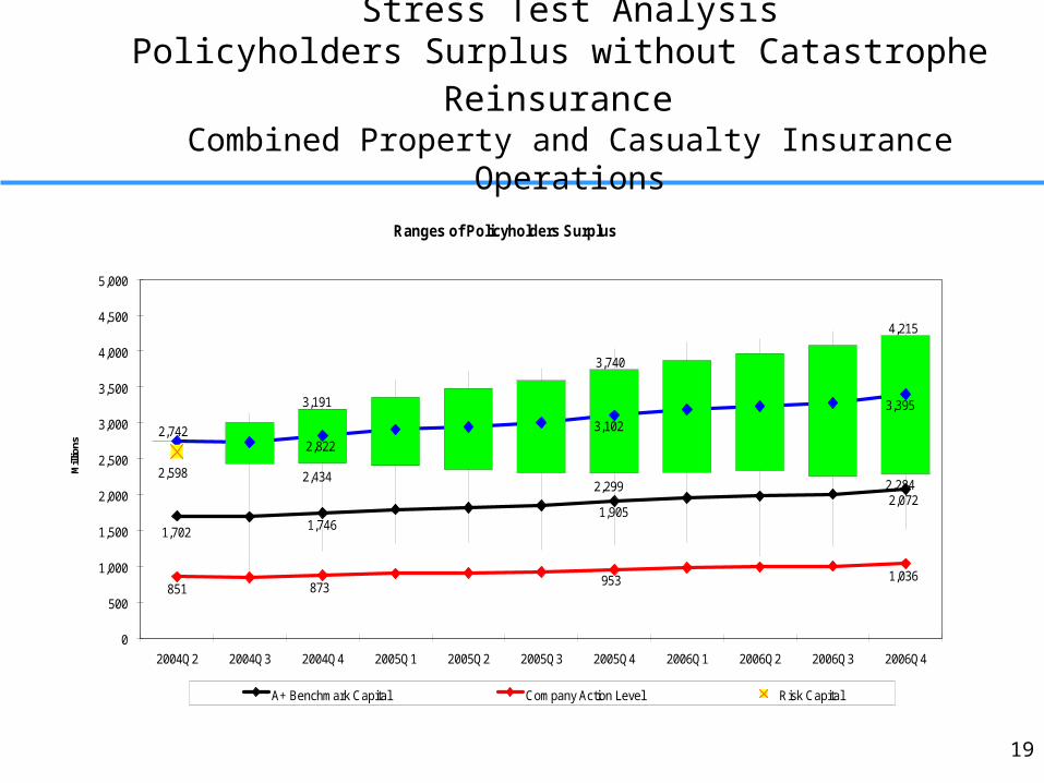
Stress Test AnalysisPolicyholders Surplus without Catastrophe Reinsurance
Combined Property and Casualty Insurance Operations
Ranges of Policyholders Surplus
3,191
3,740
4,215
2,742 3,102
3,395
2,822
2,2842,2992,434
1,9052,072
1,7461,702
1,036953873851
2,598
0
500
1,000
1,500
2,000
2,500
3,000
3,500
4,000
4,500
5,000
2004Q2 2004Q3 2004Q4 2005Q1 2005Q2 2005Q3 2005Q4 2006Q1 2006Q2 2006Q3 2006Q4
Mill
ions
A+ Benchmark Capital Company Action Level Risk Capital
20
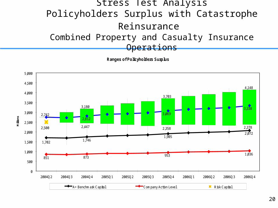
Stress Test AnalysisPolicyholders Surplus with Catastrophe Reinsurance
Combined Property and Casualty Insurance Operations
Ranges of Policyholders Surplus
3,180
3,703
4,148
2,742 3,069
3,338
2,812
2,3782,3582,447
1,9052,072
1,7461,702
1,036953873851
2,500
0
500
1,000
1,500
2,000
2,500
3,000
3,500
4,000
4,500
5,000
2004Q2 2004Q3 2004Q4 2005Q1 2005Q2 2005Q3 2005Q4 2006Q1 2006Q2 2006Q3 2006Q4
Mill
ions
A+ Benchmark Capital Company Action Level Risk Capital
21
Stress Test Analysis - Summary Risk Assessment of Catastrophe Reinsurance
Property and Casualty Insurance Operations
• Risk assessment of the purchase of Catastrophe Reinsurance over the next 2½ years– Risk Capital
• With Cat Reinsurance $2,500 mil
• Without Cat Reinsurance $2,598 mil
• Impact of Cat Reinsurance $98 mil
– Average PHS at the end of simulation period• With Cat Reinsurance $3,338 mil
• Without Cat Reinsurance $3,395 mil
• Impact of Cat Reinsurance $57 mil
– Conclusion• Combined P&C operations has enough capital to self insure against
catastrophes given a risk tolerance of .0025% and a time horizon of 2 ½ years
22
Analysis of Reinsurance Buying Options
23
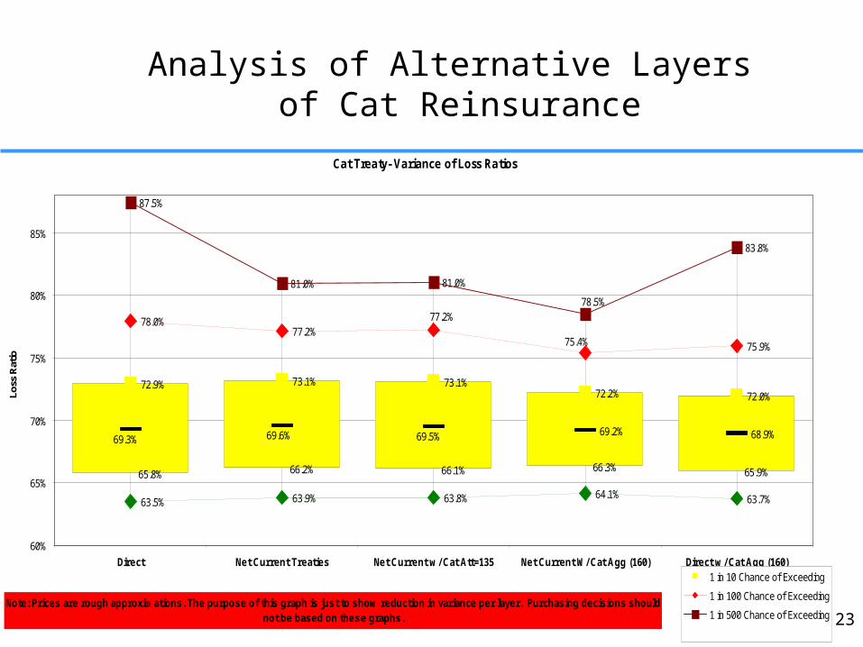
Analysis of Alternative Layers of Cat Reinsurance
Cat Treaty- Variance of Loss Ratios
72.9% 73.1% 73.1%72.2% 72.0%
78.0%77.2%
75.9%
69.2% 68.9%
63.5% 63.9% 63.8% 64.1% 63.7%
87.5%
81.0% 81.0%
83.8%
65.8% 66.2% 66.1% 66.3% 65.9%
77.2%
75.4%
69.5%69.6%69.3%
78.5%
60%
65%
70%
75%
80%
85%
Direct Net Current Treaties Net Current w/ Cat Att=135 Net Current W/ Cat Agg (160) Direct w/ Cat Agg (160)
Note: Prices are rough approximations. The purpose of this graph is just to show reduction in variance per layer. Purchasing decisions should not be based on these graphs.
Loss
Rat
io
1 in 10 Chance of Exceeding
1 in 100 Chance of Exceeding
1 in 500 Chance of Exceeding
24
Example of Analysis of Capital Allocation and Risk / Reward Alternatives
25
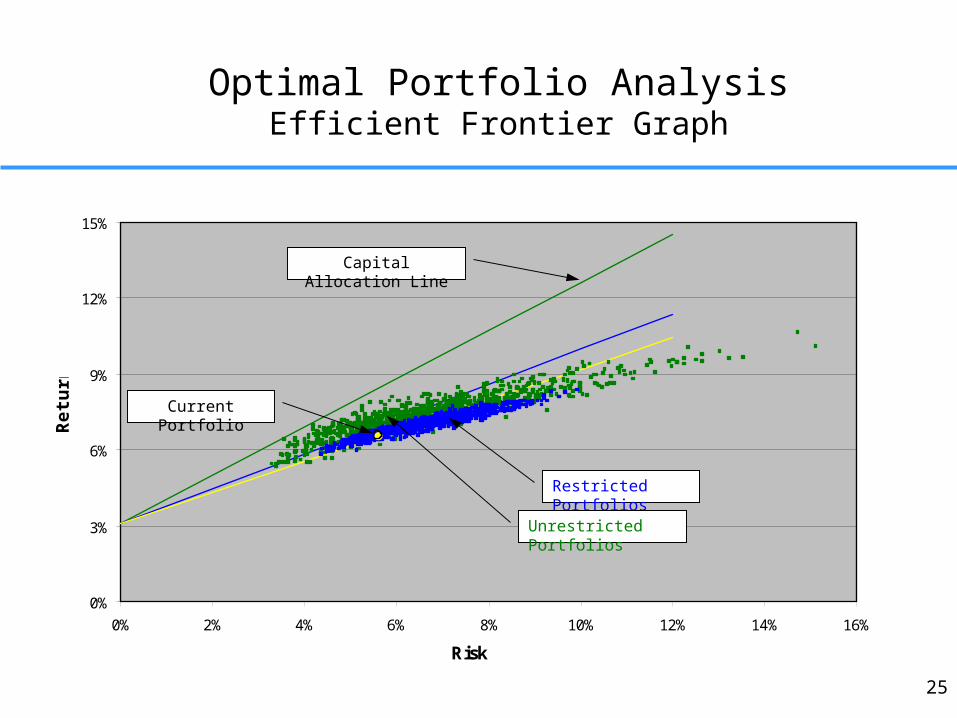
Optimal Portfolio AnalysisEfficient Frontier Graph
0%
3%
6%
9%
12%
15%
0% 2% 4% 6% 8% 10% 12% 14% 16%
Risk
Ret
urn
Restricted Portfolios
Unrestricted Portfolios
Capital Allocation Line
Current Portfolio
26
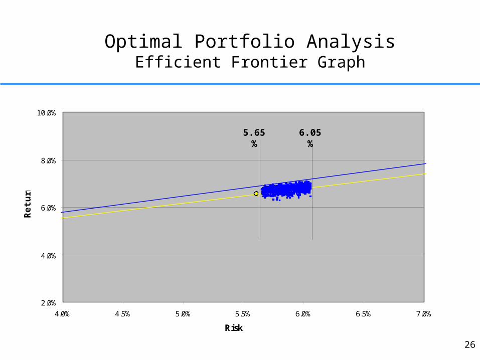
Optimal Portfolio AnalysisEfficient Frontier Graph
2.0%
4.0%
6.0%
8.0%
10.0%
4.0% 4.5% 5.0% 5.5% 6.0% 6.5% 7.0%
Risk
Ret
urn
5.65% 6.05%
27
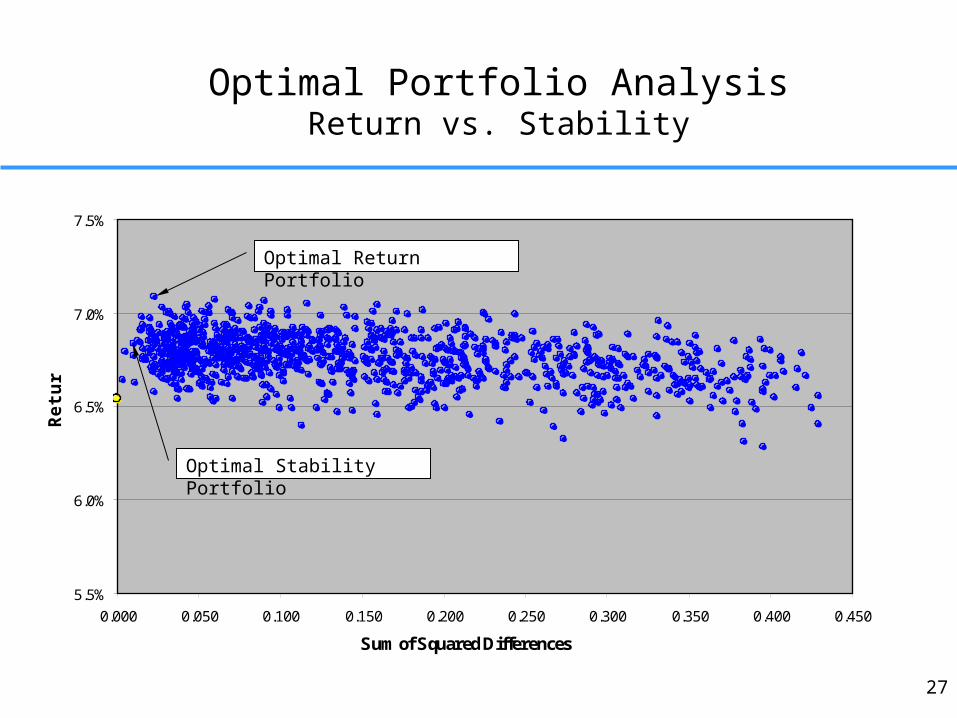
Optimal Portfolio AnalysisReturn vs. Stability
5.5%
6.0%
6.5%
7.0%
7.5%
0.000 0.050 0.100 0.150 0.200 0.250 0.300 0.350 0.400 0.450
Sum of Squared Differences
Ret
urn
Optimal Stability Portfolio
Optimal Return Portfolio
28
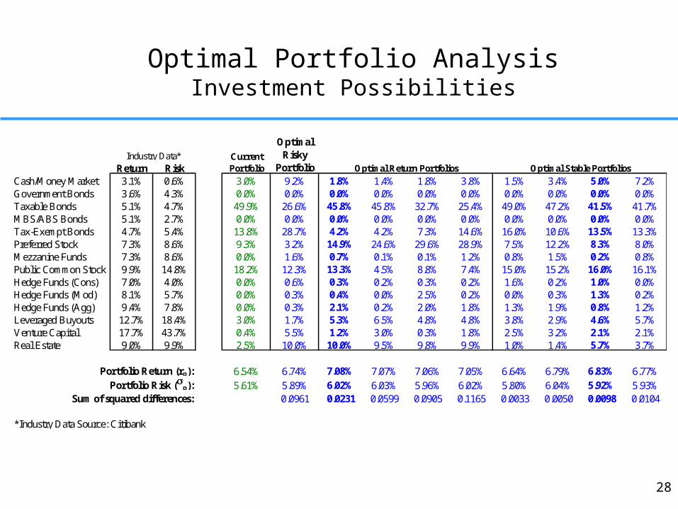
Optimal Portfolio AnalysisInvestment Possibilities
Return RiskCash/Money Market 3.1% 0.6% 3.0% 9.2% 1.8% 1.4% 1.8% 3.8% 1.5% 3.4% 5.0% 7.2%Government Bonds 3.6% 4.3% 0.0% 0.0% 0.0% 0.0% 0.0% 0.0% 0.0% 0.0% 0.0% 0.0%Taxable Bonds 5.1% 4.7% 49.9% 26.6% 45.8% 45.8% 32.7% 25.4% 49.0% 47.2% 41.5% 41.7%MBS/ABS Bonds 5.1% 2.7% 0.0% 0.0% 0.0% 0.0% 0.0% 0.0% 0.0% 0.0% 0.0% 0.0%Tax-Exempt Bonds 4.7% 5.4% 13.8% 28.7% 4.2% 4.2% 7.3% 14.6% 16.0% 10.6% 13.5% 13.3%Preferred Stock 7.3% 8.6% 9.3% 3.2% 14.9% 24.6% 29.6% 28.9% 7.5% 12.2% 8.3% 8.0%Mezzanine Funds 7.3% 8.6% 0.0% 1.6% 0.7% 0.1% 0.1% 1.2% 0.8% 1.5% 0.2% 0.8%Public Common Stock 9.9% 14.8% 18.2% 12.3% 13.3% 4.5% 8.8% 7.4% 15.0% 15.2% 16.0% 16.1%Hedge Funds (Cons) 7.0% 4.0% 0.0% 0.6% 0.3% 0.2% 0.3% 0.2% 1.6% 0.2% 1.0% 0.0%Hedge Funds (Mod) 8.1% 5.7% 0.0% 0.3% 0.4% 0.0% 2.5% 0.2% 0.0% 0.3% 1.3% 0.2%Hedge Funds (Agg) 9.4% 7.8% 0.0% 0.3% 2.1% 0.2% 2.0% 1.8% 1.3% 1.9% 0.8% 1.2%Leveraged Buyouts 12.7% 18.4% 3.0% 1.7% 5.3% 6.5% 4.8% 4.8% 3.8% 2.9% 4.6% 5.7%Venture Capital 17.7% 43.7% 0.4% 5.5% 1.2% 3.0% 0.3% 1.8% 2.5% 3.2% 2.1% 2.1%Real Estate 9.0% 9.9% 2.5% 10.0% 10.0% 9.5% 9.8% 9.9% 1.0% 1.4% 5.7% 3.7%
Portfolio Return (rp): 6.54% 6.74% 7.08% 7.07% 7.06% 7.05% 6.64% 6.79% 6.83% 6.77%Portfolio Risk (p): 5.61% 5.89% 6.02% 6.03% 5.96% 6.02% 5.80% 6.04% 5.92% 5.93%
Sum of squared differences: 0.0961 0.0231 0.0599 0.0905 0.1165 0.0033 0.0050 0.0098 0.0104
*Industry Data Source: Citibank
Optimal Return Portfolios Optimal Stable PortfoliosIndustry Data* Current
Portfolio
Optimal Risky
Portfolio
29
Analysis of Incentive Compensation Goals
30
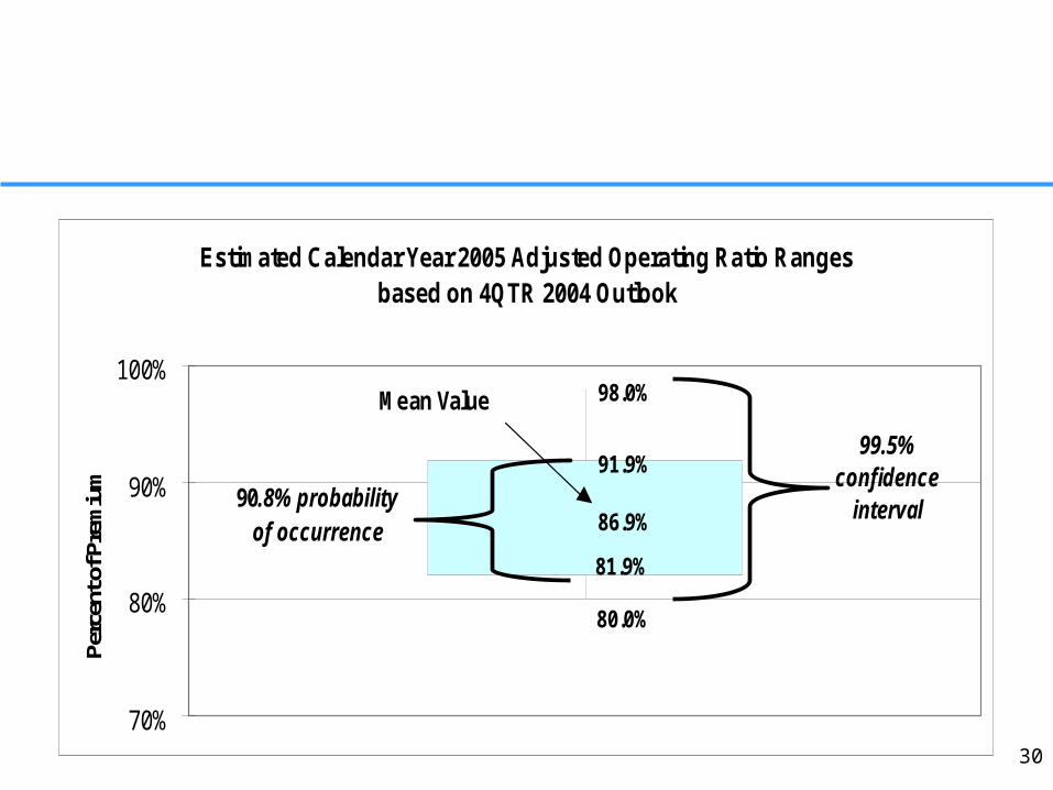
Estimated Calendar Year 2005 Adjusted Operating Ratio Rangesbased on 4QTR 2004 Outlook
86.9%
98.0%
91.9%
81.9%
80.0%
70%
80%
90%
100%
Perc
ent o
f Pre
miu
m
99.5% confidence
interval 90.8% probability of occurrence
Mean Value
31
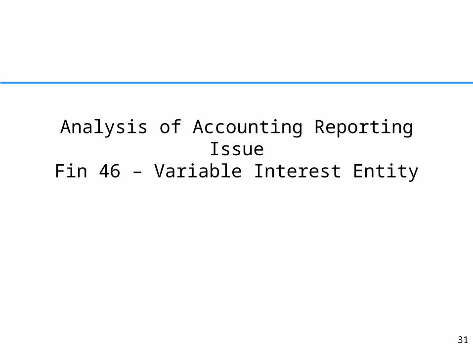
Analysis of Accounting Reporting IssueFin 46 – Variable Interest Entity
32
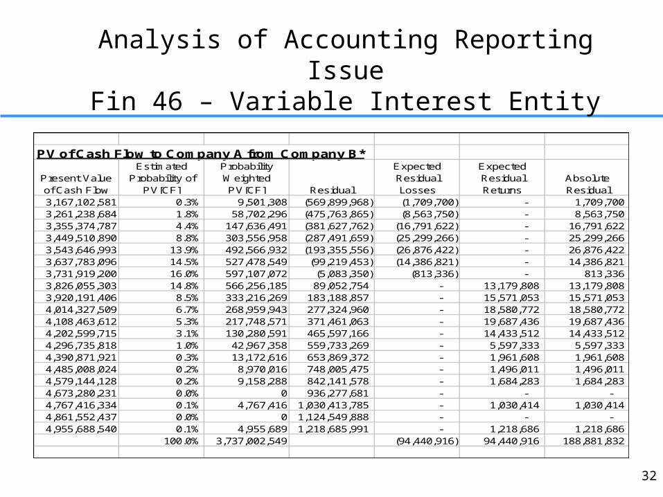
Analysis of Accounting Reporting IssueFin 46 – Variable Interest Entity
PV of Cash Flow to Company A from Company B*
Present Value of Cash Flow
Estimated Probability of
PV[CF]
Probability Weighted PV[CF] Residual
Expected Residual Losses
Expected Residual Returns
Absolute Residual
3,167,102,581 0.3% 9,501,308 (569,899,968) (1,709,700) - 1,709,700 3,261,238,684 1.8% 58,702,296 (475,763,865) (8,563,750) - 8,563,750 3,355,374,787 4.4% 147,636,491 (381,627,762) (16,791,622) - 16,791,622 3,449,510,890 8.8% 303,556,958 (287,491,659) (25,299,266) - 25,299,266 3,543,646,993 13.9% 492,566,932 (193,355,556) (26,876,422) - 26,876,422 3,637,783,096 14.5% 527,478,549 (99,219,453) (14,386,821) - 14,386,821 3,731,919,200 16.0% 597,107,072 (5,083,350) (813,336) - 813,336 3,826,055,303 14.8% 566,256,185 89,052,754 - 13,179,808 13,179,808 3,920,191,406 8.5% 333,216,269 183,188,857 - 15,571,053 15,571,053 4,014,327,509 6.7% 268,959,943 277,324,960 - 18,580,772 18,580,772 4,108,463,612 5.3% 217,748,571 371,461,063 - 19,687,436 19,687,436 4,202,599,715 3.1% 130,280,591 465,597,166 - 14,433,512 14,433,512 4,296,735,818 1.0% 42,967,358 559,733,269 - 5,597,333 5,597,333 4,390,871,921 0.3% 13,172,616 653,869,372 - 1,961,608 1,961,608 4,485,008,024 0.2% 8,970,016 748,005,475 - 1,496,011 1,496,011 4,579,144,128 0.2% 9,158,288 842,141,578 - 1,684,283 1,684,283 4,673,280,231 0.0% 0 936,277,681 - - - 4,767,416,334 0.1% 4,767,416 1,030,413,785 - 1,030,414 1,030,414 4,861,552,437 0.0% 0 1,124,549,888 - - - 4,955,688,540 0.1% 4,955,689 1,218,685,991 - 1,218,686 1,218,686
100.0% 3,737,002,549 (94,440,916) 94,440,916 188,881,832
33
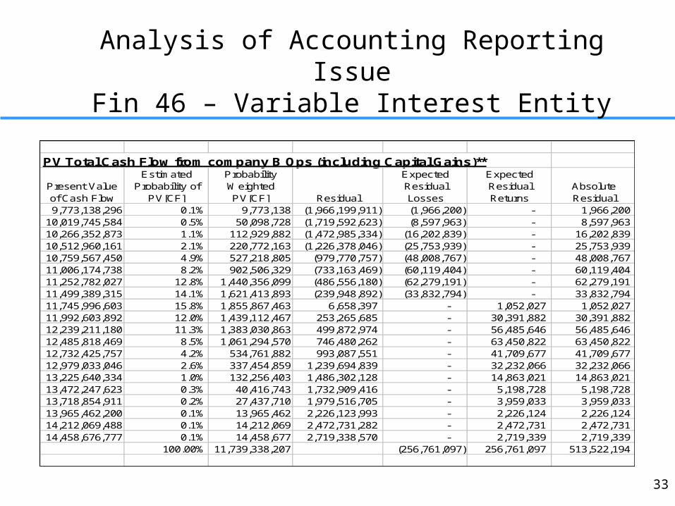
Analysis of Accounting Reporting IssueFin 46 – Variable Interest Entity
PV Total Cash Flow from company B Ops (including Capital Gains)**
Present Value of Cash Flow
Estimated Probability of
PV[CF]
Probability Weighted PV[CF] Residual
Expected Residual Losses
Expected Residual Returns
Absolute Residual
9,773,138,296 0.1% 9,773,138 (1,966,199,911) (1,966,200) - 1,966,200 10,019,745,584 0.5% 50,098,728 (1,719,592,623) (8,597,963) - 8,597,963 10,266,352,873 1.1% 112,929,882 (1,472,985,334) (16,202,839) - 16,202,839 10,512,960,161 2.1% 220,772,163 (1,226,378,046) (25,753,939) - 25,753,939 10,759,567,450 4.9% 527,218,805 (979,770,757) (48,008,767) - 48,008,767 11,006,174,738 8.2% 902,506,329 (733,163,469) (60,119,404) - 60,119,404 11,252,782,027 12.8% 1,440,356,099 (486,556,180) (62,279,191) - 62,279,191 11,499,389,315 14.1% 1,621,413,893 (239,948,892) (33,832,794) - 33,832,794 11,745,996,603 15.8% 1,855,867,463 6,658,397 - 1,052,027 1,052,027 11,992,603,892 12.0% 1,439,112,467 253,265,685 - 30,391,882 30,391,882 12,239,211,180 11.3% 1,383,030,863 499,872,974 - 56,485,646 56,485,646 12,485,818,469 8.5% 1,061,294,570 746,480,262 - 63,450,822 63,450,822 12,732,425,757 4.2% 534,761,882 993,087,551 - 41,709,677 41,709,677 12,979,033,046 2.6% 337,454,859 1,239,694,839 - 32,232,066 32,232,066 13,225,640,334 1.0% 132,256,403 1,486,302,128 - 14,863,021 14,863,021 13,472,247,623 0.3% 40,416,743 1,732,909,416 - 5,198,728 5,198,728 13,718,854,911 0.2% 27,437,710 1,979,516,705 - 3,959,033 3,959,033 13,965,462,200 0.1% 13,965,462 2,226,123,993 - 2,226,124 2,226,124 14,212,069,488 0.1% 14,212,069 2,472,731,282 - 2,472,731 2,472,731 14,458,676,777 0.1% 14,458,677 2,719,338,570 - 2,719,339 2,719,339
100.00% 11,739,338,207 (256,761,097) 256,761,097 513,522,194
34
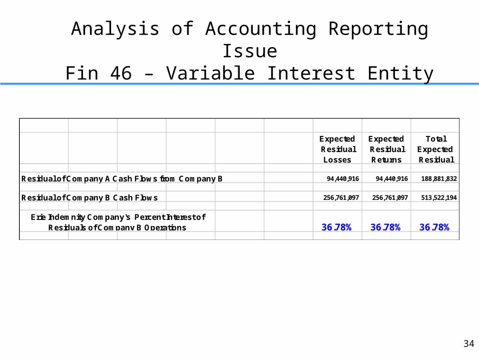
Analysis of Accounting Reporting IssueFin 46 – Variable Interest Entity
Expected Residual Losses
Expected Residual Returns
Total Expected Residual
Residual of Company A Cash Flows from Company B 94,440,916 94,440,916 188,881,832
Residual of Company B Cash Flows 256,761,097 256,761,097 513,522,194
36.78% 36.78% 36.78%Erie Indemnity Company's Percent Interest of
Residuals of Company B Operations

![[PPT]PowerPoint Presentation - Event Schedule & Agenda …schd.ws/hosted_files/2016agripspring/97/Joint ERM... · Web viewOutline ERM Frameworks Why CIS is Involved in ERM CIS ERM](https://static.fdocuments.us/doc/165x107/5ac13a447f8b9a4e7c8cc305/pptpowerpoint-presentation-event-schedule-agenda-schdwshostedfiles2016agripspring97joint.jpg)