PRACTICAL CONSIDERATIONS FOR RADAR

EMBEDDED COMMUNICATION

by

Casey Biggs

Submitted to the graduate degree program in Electrical Engineering & Computer

Science and the Graduate Faculty of the University of Kansas School of Engineering

in partial fulfillment of the requirements for the degree of Master of Science.

Thesis Committee:

__________________________________________Dr. Shannon D. Blunt (Chair)__________________________________________Dr. Christopher Allen__________________________________________Dr. Erik Perrins__________________________________________Date of Thesis Defense

1st July 2009

The thesis committee for Casey Biggs certifies that

this is the approved version of the following thesis:

PRACTICAL CONSIDERATIONS FOR RADAR EMBEDDED

COMMUNICATION

__________________________________________Dr. Shannon D. Blunt (Chair)

__________________________________________Dr. Christopher Allen

__________________________________________Dr. Erik Perrins

__________________________________________Date Approved

ii

1st July 2009

Acknowledgements

I would first like to thank my advisor Dr. Shannon Blunt for his continued

guidance and support in understanding and advancing this research and writing this

thesis. I would like to thank the Air Force Office of Scientific Research (AFOSR) for

sponsoring the research. Special thanks to Dr. Christopher Allen and Dr. Erik Perrins

for agreeing to be on my thesis committee. I would also like to thank my professors

and classmates for making my return to school enjoyable. Last, but not least, I would

like to thank my family and friends for their support through this busy time.

iii

Table of Contents

Title Page........................................................................................................................i

Acceptance Page............................................................................................................ii

Acknowledgements......................................................................................................iii

Table of Contents..........................................................................................................iv

Abstract..........................................................................................................................1

CHAPTER 1: INTRODUCTION..................................................................................2

1.1 MOTIVATION OF THESIS...............................................................................3

1.2 ORGANIZATION OF THESIS.........................................................................6

CHAPTER 2: BACKGROUND....................................................................................7

2.1 WAVEFORM DESIGN......................................................................................9

2.1.1 EIGENVECTORS-AS-WAVEFORMS....................................................11

2.1.2 WEIGHTED-COMBINING.....................................................................12

2.1.3 DOMINANT-PROJECTION...................................................................13

2.2 RECEIVER DESIGN.......................................................................................14

CHAPTER 3: WAVEFORM MISMATCHES BETWEEN TAG AND RECEIVER. .17

3.1 FORWARD SCATTERING (MULTIPATH)...................................................19

3.1.1 IMPULSE AND AWGN...........................................................................21

3.1.2 IMPULSIVE CHANNEL.........................................................................24

3.1.3 MANY RANDOM IMPULSES (SEVERE MULTIPATH).....................25

3.1.4 ROBUSTNESS OF DOMINANT-PROJECTION...................................27

3.2 WAVEFORM LENGTH DIFFERENCES.......................................................39

iv

3.3 SAMPLING RATE DIFFERENCES...............................................................46

CHAPTER 4: SYNCHRONIZATION ISSUES..........................................................50

4.1 SER PERFORMANCE SEARCHING OVER TIME.....................................52

4.2 THREE SAMPLE AVERAGE.........................................................................53

4.3 SYMBOLS WITH LESS LOCAL CROSS-CORRELATION........................55

4.4 DISTRIBUTION OF FILTER OUTPUTS......................................................59

4.5 MULTIPATH AND SYNCHRONIZATION....................................................69

4.6 INTERCEPT RECEIVER SYNCHRONIZATION.........................................74

CHAPTER 5: IMPROVING WAVEFORM DESIGN.................................................78

5.1 TEMPORAL EXPANSION.............................................................................78

5.1.1 SER PERFORMANCE WITH TEMPORAL EXPANSION...................79

5.1.2 ADDED DIMENSIONALITY OF TEMPORAL EXPANSION.............80

5.1.3 TEMPORAL AND BANDWIDTH EXPANSION TRADE-OFF...........81

5.2 SYMBOL WAVEFORMS WITH LESS CROSS-CORRELATION...............83

5.2.1 WEIGHTED DOMINANT PROJECTION.............................................83

5.2.2 DOMINANT-PROJECTION WITH GRAM-SCHMITT........................86

5.2.3 FAILURE TO IMPROVE SER................................................................89

5.3 EQUALIZING INTERFERENCE LEVELS AMONG SYMBOLS...............90

5.4 ADJUSTING SYMBOL CORRELATION WITH CLUTTER.......................93

CHAPTER 6: CONCLUSIONS AND FUTURE WORK...........................................97

FUTURE WORK....................................................................................................99

References..................................................................................................................101

v

Abstract

This thesis expands on the previous work done in the area of intra-pulse radar

embedded communication by examining some of the practical aspects of the

waveform design. Communication waveform mismatches between the tag and

receiver due to multipath distortion, sampling rate differences and using different

lengths for the radar waveform are explored for each of the three previously

developed design methods. The Dominant-Projection approach is shown to be robust

to most mismatches while the other two approaches significantly degrade or fail with

any mismatch. Lack of synchronization between the receiver and tag is shown to

increase the occurrence of symbol errors, since the receiver is required to search over

multiple samples for the communication waveform sent by the tag. Attempts to

reduce the number of errors caused by the lack of synchronization are also made, first

by taking a three sample average of the filter output and second by generating

waveforms with lower local cross-correlation, with both attempts shown to be

unsuccessful. Other attempts are also made to improve the waveform design. It is

shown that temporal expansion can be used to either improve symbol error rate or

reduce the amount of bandwidth expansion required. A rule-of-thumb is developed for

the bandwidth expansion versus temporal expansion trade-off. It is also shown that

more of the dominant space can be projected out with Dominant-Projection to reduce

the probability of symbol error, but this comes at the cost of being more susceptible to

being detected by an intercept receiver.

1

CHAPTER 1

INTRODUCTION

The ability to communicate without interception can at times be highly

desirable, especially in military applications. Previously, systems have been deployed

that embed communication signals into the backscatter of radar by operating on a

pulse to pulse basis to achieve covert communication, but at a low data rate. Previous

work in [1]-[4] develops symbol waveforms that work instead on an intra-pulse basis

to achieve a higher data rate than the inter-pulse methods while still remaining covert.

In this thesis, some of the practical aspects of an intra-pulse radar embedded

communication system are discussed and the three symbol waveform designs are

tested to see how they perform in more real world situations. Also, the

communication waveform design is explored and modified in an attempt to reduce the

symbol error rate (SER) while maintaining a low probability of intercept (LPI).

In a radar system, a transmitter sends out a radio frequency (RF) signal

(pulsed or continuous) that scatters off objects that it encounters. A receiver collects

the scattered signal to determine information (range, velocity, cross-section, etc.)

about the illuminated objects [5]. An RF tag/transponder that is illuminated by the

radar can embed a communication signal in its backscatter by remodulating the

incident waveform. To be effective, the communication waveforms need to be similar

enough to the ambient scattering of the radar signal to be difficult to intercept, yet

separable enough from the clutter to be detected by an intended receiver with a low

2

probability of symbol error.

Three design methods were previously developed to generate the symbol

waveforms for intra-pulse communication. Each method utilizes that the spectrum of

most radar signals spread out beyond their passband. This “bleeding” spectrum of the

radar waveform is used as expanded bandwidth for the communication waveforms to

reside. Also, each method uses the eigenvectors from a correlation matrix based on

the ambient scattering of the radar signal to produce communication waveforms that

are partially correlated with the clutter in an effort to be more hidden.

1.1 MOTIVATION OF THESIS

The motivation of this thesis is to examine some of the practical aspects of

intra-pulse radar embedded communication when using the three previously

developed waveform design approaches in [1]-[4]. Also, attempts to improve

waveform and receiver design are explored in order to achieve a higher symbol error

rate and/or to have the communication signal be more hidden and thus have a lower

probability of intercept.

Each of the communication waveform design methods use the incident radar

signal at the tag in the symbol generation process to produce waveforms that are

partially correlated with the ambient scattering. A tag or receiver that is not co-located

with the radar would first need to sample the incident radar waveform. Mismatches in

the sampled radar waveform could then result in communication waveforms

generated at the tag that are different than the waveforms generated at the receiver.

3

Three situations that would cause changes in the sampled radar waveform are

explored by examining the effect of those differences on the resulting communication

waveforms. The first scenario considered is distortion of the incident radar waveform

by forward scatter (i.e. multipath). A tag (or remote receiver) could receive multiple

copies of the transmitted radar waveform due to reflections off objects being

illuminated by the radar. The multiple copies received from the multipath channel can

also cause the radar waveform to appear longer, making it difficult to determine the

exact length of the transmitted waveform. The second mismatch situation explored is

then when the tag and receiver determine different lengths for the sampled radar

waveform used in the symbol generation, but without distortion. The last mismatch

that is considered occurs from the tag and receiver using different sampling rates for

the incident radar waveform.

The second practical aspect considered is when the receiver is not

synchronized with the symbol waveform sent by the tag. The simulations to

determine the probability of symbol error, performed previously in [1]-[4], assumed

that the receiver had exact knowledge of the time delay of the embedded

communication signal. The receiver could then use the filter output at the match point

to determine the most likely symbol sent. If the time delay is not known, the receiver

would need to search over multiple samples to extract the embedded symbol,

increasing the probability of a symbol error.

Attempts will also be made to improve the waveform design with the goal of

reducing errors and/or the probability of intercept. In order to improve performance,

4

the time length, as well as the bandwidth, of the radar waveform can be expanded as

added dimensionality for communication waveform design. A rule-of-thumb is then

developed for the trade-off between temporal and bandwidth expansion for a given

symbol error rate. The second attempt at improving waveform design is to modify the

Dominant-Projection approach to generate symbols that have less cross-correlation.

This is achieved with two different methods. The first is giving a larger weight to the

previously generated symbol waveforms in the projection matrix when generating

new symbols and the second is combining the approach with the Gram-Schmitt

procedure. The third attempt at improving performance is to equalize the correlation

of the symbol waveforms with the interference by using the Hadamard transform.

This is done to remove any symbol biases in the receiver caused by some symbols

having a higher correlation with the interference than other symbols. The final

method explored for improving the symbol waveform design to reduce symbol errors

is accomplished by adjusting the size of the non-dominant space used when

generating the symbols with Dominant-Projection. When the size of the non-

dominant space is reduced, more of the dominant space will be projected away and

the communication waveforms will be less correlated with the clutter interference. As

a result, less symbol errors should occur. However, reducing the correlation of the

communication waveforms with the interference would also make them less hidden

thus increasing the probability of intercept by an unintended receiver.

5

1.2 ORGANIZATION OF THESIS

The remainder of thesis is organized into the following chapters. Chapter 2

covers some of the background on radar-embedded communication, specifically

covering the previous work on intra-pulse coding. In chapter 3, situations that may

cause mismatches in the communication waveforms used by the tag and receiver are

explored. Receiver synchronization issues are examined in chapter 4 with two

methods explored for reducing the effect of a lack of synchronization. Attempts to

improve communication waveform design are discussed in chapter 5. Conclusions

and future work to be performed are presented in chapter 6.

6

CHAPTER 2

BACKGROUND

The foundation for radar embedded communication beyond on-off signaling

started in 1948 with Stockman's idea of using mechanically controlled corner

reflectors to modulate the backscatter radiation [6]. More information could then be

conveyed from the target back to the receiver by changing the reflector over multiple

pulses. This idea was then expanded upon to develop more methods to use modulated

reflectors as a means of communication. The majority of the methods developed for

embedding communication signals in radar backscatter involved changing the

modulation from pulse to pulse. In [7]-[11], a phase-shift sequence is applied to the

reflections over multiple pulses. The phase-shifts can be imparted in a way that, to an

unintended receiver that does not know the sequence, the phase modulation appears

to be a Doppler signature. This approach allows the communication to be covert.

These inter-pulse modulation techniques, though, often require on the order of

hundreds of pulses for the symbol sequence. This results in a low data rate on the

order of bits per coherent processing interval (CPI), which translates to a throughput

of only a couple of bits per second (bps).

By operating on a intra-pulse basis, the incident radar waveform is

remodulated into one of K different symbol waveforms. This allows transmission

on the order of a few bits per pulse. Therefore, a radar having a pulse repetition

7

frequency (PRF) in the kHz range would have a communication rate on the order of

kilobits per second (kbps). This greatly increases the amount of data that can be sent

and if the communication waveforms are properly designed, can still have a low

probability of intercept.

In [12], convolutional coding is used as an intra-pulse technique to remodulate

the incident waveform. This modulation can achieve data rates up to 256 kbps, but the

convolution coding uses the same mathematical structure as physical scattering. This

process would initially appear to have a higher probability of intercept, since standard

radar detection could most likely be used to intercept the embedded symbol

waveforms. More work is needed to compare the convolution modulation with the

design approaches discussed below.

The intra-pulse waveform design methods developed in [1]-[4], which are

further explored and expanded in this thesis, utilize the spectrum of the radar signal

outside its passband as a place to embed a communication signal. Expanding the

bandwidth of the radar waveform provides a design space for the communication

waveforms. The waveforms are designed to be similar to the ambient scattering of the

radar making them harder to detect and more covert, but separable enough at the

intended receiver to have a low probability of symbol error. The design of the

communication waveforms is further discussed in the next section.

8

2.1 WAVEFORM DESIGN

As discussed above, the three intra-pulse waveform design approaches take

advantage of the spectral bleeding of the radar signal for embedding covert

communication signals. This spreading of the radar spectrum is shown below in

figure 2.1.1. Since the radar occupies its entire passband, expanding into this bleeding

region provides space to design the communication waveforms. In order for the

communication waveforms to have a low probability of intercept (LPI), each of the

three design methods generate waveforms that are partially correlated with the

ambient scattering of the radar signal. This similarity allows the communication

waveforms to be better hidden by the interference. The process of generating the

symbol waveforms to be similar to the ambient scattering is further discussed below.

Figure 2.1.1: Radar spectral “bleeding” effect.

9

First, let s t be the transmitted radar waveform. Oversampling this

waveform by a factor of M results in the NM length vector s=[s0 s1 sNM−1]T ,

where N is the length of the radar waveform when sampled at Nyquist and ⋅T is

the transpose operation. The ambient scattering of the radar waveform could then be

modeled as

Sx=[sNM−1 s NM−2 ⋯ s0 0 ⋯ 0

0 s NM−1 ⋯ s1 s0 ⋯ 0⋮ ⋮ ⋱ ⋮ ⋮ ⋱ ⋮0 0 ⋯ s NM−1 sNM−2 ⋯ s0

]x (2.1)

where the NM×2 NM−1 matrix S is the the set of 2 NM−1 possible delay

shifts of the sampled incident radar waveform s and the vector x is the range

profile of the ambient scattering. A convenient basis for the generation of the

communication waveforms is obtained from the eigen-decomposition of the

correlation of S as

SS H=V V H (2.2)

where V=[v0 v1 vNM−1] are the NM eigenvectors, is a diagonal matrix of

the associated eigenvalues (in order of decreasing magnitude) and ⋅H is the

Hermitian operator. Figure 2.1.2 shows a plot of the eigenvalues of SS H with a

linear frequency modulated (LFM) waveform oversampled by a factor of M=2 . In

the plot, we see that the eigenvalues are roughly divided into dominant and non-

dominant spaces, but there is a similar “bleeding” of values into the non-dominant

space. The Eigenvectors-as-Waveforms, Weighted-Combining and Dominant-

10

Projection waveform design approaches utilize the non-dominant space for the

communication waveforms. Each uses a different method of using the eigenvectors of

SSH to generate the K symbols ck .

Figure 2.1.2: Eigenvalue plot with the radar waveform oversampled by 2.

2.1.1 EIGENVECTORS-AS-WAVEFORMS

The simplest design method uses a subset of the individual eigenvectors of the

correlation matrix SS H for the communication waveforms. The least dominant

eigenvectors are used such that each will have equal interference with the radar

scattering. The communication waveforms are then the eigenvectors with the smallest

eigenvalues as

ck=v NM− k for k=1K. (2.3)

The resulting waveforms occupy a narrow bandwidth outside of the radar spectrum

and have low correlation with the clutter interference. Due to this, the Eigenvectors-

11

as-Waveforms approach has the best performance in terms of symbol error rate, but it

is also easy for an intercept receiver to detect and is the worst performer in terms of

having a low probability of intercept (LPI).

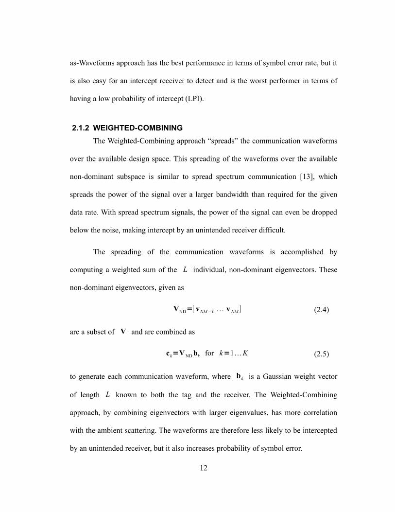
2.1.2 WEIGHTED-COMBINING

The Weighted-Combining approach “spreads” the communication waveforms

over the available design space. This spreading of the waveforms over the available

non-dominant subspace is similar to spread spectrum communication [13], which

spreads the power of the signal over a larger bandwidth than required for the given

data rate. With spread spectrum signals, the power of the signal can even be dropped

below the noise, making intercept by an unintended receiver difficult.

The spreading of the communication waveforms is accomplished by

computing a weighted sum of the L individual, non-dominant eigenvectors. These

non-dominant eigenvectors, given as

VND=[ vNM−L v NM ] (2.4)

are a subset of V and are combined as

ck=VND bk for k=1K (2.5)

to generate each communication waveform, where bk is a Gaussian weight vector

of length L known to both the tag and the receiver. The Weighted-Combining

approach, by combining eigenvectors with larger eigenvalues, has more correlation

with the ambient scattering. The waveforms are therefore less likely to be intercepted

by an unintended receiver, but it also increases probability of symbol error.

12

2.1.3 DOMINANT-PROJECTION

Instead of directly using the non-dominant eigenvectors to generate the

communication waveforms he Dominant-Projection approach a projects away from

the eigenvectors corresponding to the dominant space resulting in waveforms spread

across the entire non-dominant space. Since the dominant space is used as a whole,

the approach is less susceptible to changes in the individual indexed eigenvectors

used in the other two approaches. The Dominant-Projection design method also

spreads the communication waveform over the design space resulting in a similar

symbol error rate and probability of intercept as the Weighted-Combining approach.

In order for the communication waveforms to be separable at the receiver,

they should be designed to be pairwise orthogonal. With the other two approaches,

that use either the individual or combinations of the eigenvectors (which are each

orthogonal), the resulting communication waveforms will be orthogonal. For

Dominant-Projection, each new communication waveform needs to be projected

away from any previously generated waveform as well as the eigenvectors of the

dominant space. Therefore, when generating the k th communication waveform, any

previously generated waveform is appended to the scattering matrix S as

Sk=[S c1 ck−1] . (2.6)

The new eigen-decomposition is then

Sk SkH=V k k V k

H (2.7)

where Vk=[v k ,0 vk ,1 vk , NM−1] are the NM eigenvectors. The projection matrix

13

is generated by subtracting away the NMk−1−L eigenvectors corresponding to

the dominant space as

Pk=I− ∑i=0

NM k−L−2

vk , i v k ,iH (2.8)

where I is an NM×NM identity matrix. The size of the dominant space that is

included in the projection matrix is increased by k−1 to accommodate for the

addition of the previously generated communication waveforms that are now present

in the eigen-decomposition. Each communication waveform is generated as

c k=Pk bk (2.9)

where bk is a seed vector known to both the tag and receiver and then normalized

as

ck=c k

∥c k∥. (2.10)

2.2 RECEIVER DESIGN

For radar-embedded communication, the similarity of the communication

waveforms to the radar clutter that allows for hiding the signal for covert

communication, can provide additional obstacles for the receiver design. Previous

work on the receiver design performed in [1]-[4] is outlined below.

The NM length vector of the sampled received signal (assuming

synchronization) is

r=ckS xv (2.11)

14

where ck is the communication symbol, x is a length 2 NM−1 vector of the

radar range profile of the clutter (not necessarily the same as in equation 2.1) and v

is NM samples of additive noise. Using a matched filter, the embedded

communication symbol can be determined by selecting the symbol that satisfies

k=arg{maxk

{∣ckH r∣}}. (2.12)

Due to the relative power levels needed to hide the communication waveform in the

backscatter of the radar and the correlation of the waveforms with the ambient

scattering, the high interference levels cause significant degradation in symbol error

rate performance when a matched filter is used.

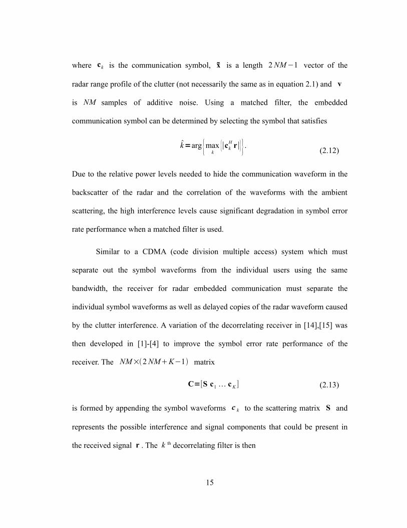
Similar to a CDMA (code division multiple access) system which must

separate out the symbol waveforms from the individual users using the same

bandwidth, the receiver for radar embedded communication must separate the

individual symbol waveforms as well as delayed copies of the radar waveform caused

by the clutter interference. A variation of the decorrelating receiver in [14],[15] was

then developed in [1]-[4] to improve the symbol error rate performance of the

receiver. The NM×2 NMK−1 matrix

C=[S c1 c K ] (2.13)

is formed by appending the symbol waveforms c k to the scattering matrix S and

represents the possible interference and signal components that could be present in

the received signal r . The k th decorrelating filter is then

15

wk=CCH−1ck for k=1,2, , K (2.14)

and equation 2.11 is changed to select the embedded waveform as

k=arg{maxk

{∣w kH r∣}} . (2.15)

With its ability to better separate out the symbol waveform from the interference, the

decorrelating filter achieves much better symbol error rate performance than when the

matched filter is used.

16

CHAPTER 3

WAVEFORM MISMATCHES BETWEEN TAG AND RECEIVER

Chapter 2 presented the three previously developed design approaches for

generating communication waveforms for intra-pulse radar embedded

communication. In each approach, the incident radar waveform is used in the

communication waveform generation process such that each symbol is sufficiently

similar to the ambient scattering. This allows for the communication waveforms to

remain hidden and to have a low probability of intercept (LPI), but separable enough

to have a viable symbol error rate. Any mismatch between the radar waveform used

by the tag and the radar waveform used by the receiver may result in the symbol

waveforms being different, thereby increasing the probability of symbol error.

Each of the three design methods for the communication waveforms start with

oversampling the incident radar waveform s t by a factor of M . This results in

the sampled radar waveform vector s=[s0 s1 s NM−1]T of length NM , where N

is the length of the radar waveform sampled at the Nyquist rate. The

NM×2 NM−1 matrix

S=[sNM−1 sNM−2 ⋯ s0 0 ⋯ 0

0 sNM−1 ⋯ s1 s0 ⋯ 0⋮ ⋮ ⋱ ⋮ ⋮ ⋱ ⋮0 0 ⋯ sNM−1 s NM−2 ⋯ s0

] (3.1)

is then the set of 2 NM−1 possible delay shifts of the sampled incident radar

17

waveform s . The three previously developed design approaches each have different

methods of using the eigenvectors of SSH to generate the K communication

waveforms ck .

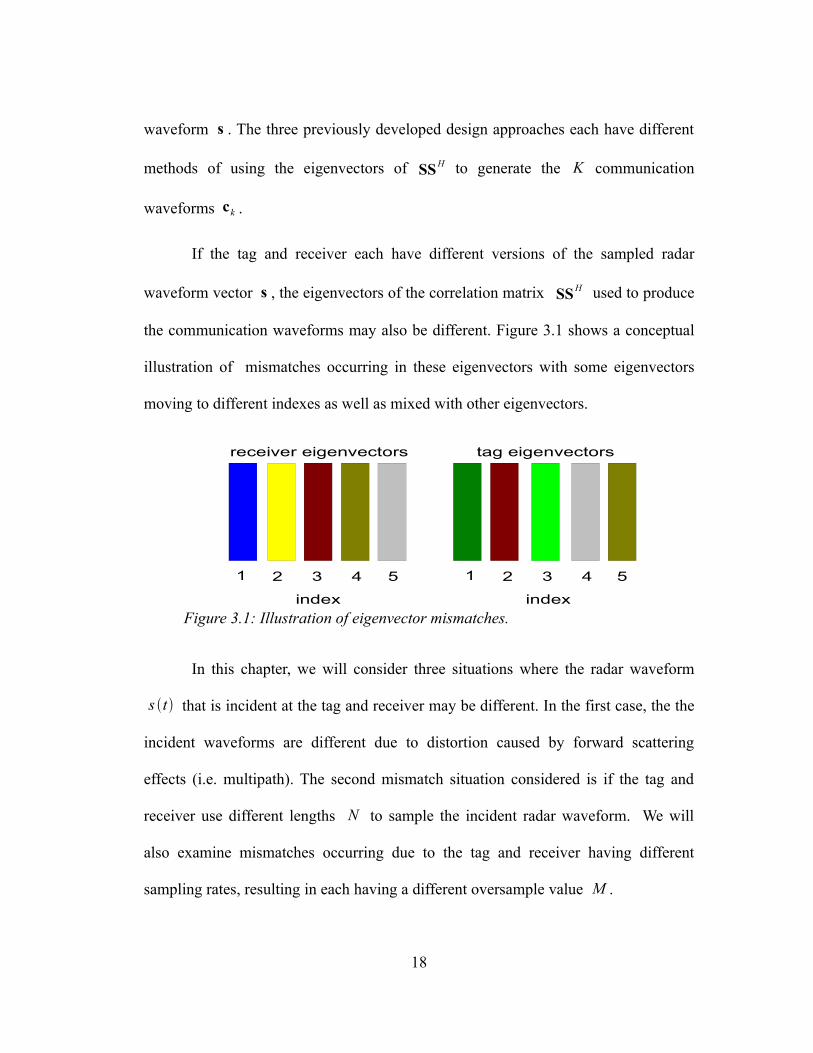
If the tag and receiver each have different versions of the sampled radar

waveform vector s , the eigenvectors of the correlation matrix SSH used to produce

the communication waveforms may also be different. Figure 3.1 shows a conceptual

illustration of mismatches occurring in these eigenvectors with some eigenvectors

moving to different indexes as well as mixed with other eigenvectors.

Figure 3.1: Illustration of eigenvector mismatches.

In this chapter, we will consider three situations where the radar waveform

s t that is incident at the tag and receiver may be different. In the first case, the the

incident waveforms are different due to distortion caused by forward scattering

effects (i.e. multipath). The second mismatch situation considered is if the tag and

receiver use different lengths N to sample the incident radar waveform. We will

also examine mismatches occurring due to the tag and receiver having different

sampling rates, resulting in each having a different oversample value M .

18

1 2 3 4 5 1 2 3 4 5

index index

receiver eigenvectors tag eigenvectors

3.1 FORWARD SCATTERING (MULTIPATH)

The radar signal incident at the tag (or a receiver not co-located with the radar)

may include multiple copies of the waveform due to reflections off objects within the

radar's illumination. An illustration of the multiple paths that the signal can travel

between the transmitter and the tag causing multiple, delayed copies of the waveform

being incident is shown in figure 3.1.1. In the radar literature, these reflections are

generally known as forward scattering; in communications, they are known as

multipath. In this section, we consider the situation in which the tag is located in a

multipath environment and the receiver is the radar receiver and thus, has the exact

waveform that is transmitted. Multipath distortion of the symbol waveforms from the

tag to the receiver will not be considered in this chapter; it will be discussed later in

section 4.5.

Figure 3.1.1: Illustration of multipath propagation.

19

To simulate the effect of the multipath environment on the radar waveform

incident at the tag, the impulse response of the channel h t is generated based on a

multipath model. The distorted radar waveform s t received at the tag is then

s t =s t ∗ht (3.2)

where ∗ is the convolution operation. Three different multipath models are

simulated: 1) an impulse at t=0 and additive white Gaussian noise, 2) the same

impulse with a second, randomly delayed impulse having a random complex

amplitude, and 3) a severe multipath scenario with many randomly delayed impulses

each with a random complex value (including the direct path component).

For the simulations in this chapter, a sampled linear frequency modulated

(LFM) radar waveform of type P3 from [16] is used with a length of N=100 . In

order to simulate the continuous nature of s t , the P3 radar waveform is

oversampled by a factor of M c=10 given as

scn=ej

N

nM c

2

(3.3)

for n=[0 1 NM c−1] , which results in the NM c length vector sc . The

oversampled version of the multipath distorted radar waveform is then

sc= sc∗h (3.4)

where h is the sampled version of the channel impulse response and ∗ is the

convolution operation. The tag truncates s c to the correct length and samples the

result to obtain s and the receiver samples the undistorted sc to obtain s , each

20

having a final oversampling rate of M=2 and length of NM=200 . The tag and

receiver use the vectors s and s to generate K=4 communication waveforms

c k and ck respectively, using the three design approaches described in sections

2.1.1-3. The Weighed-Combining and Dominant-Projection approaches use L=100

for the size of the non-dominant space. The tag transmits the communication

waveforms c k generated from the multipath distorted radar waveform and the

receiver uses the decorrelating filters wk from ck generated without multipath as in

equation (2.14), to detect the transmitted waveforms via equation (2.15).

Monte Carlo simulations are run simulating 10,000 symbol transmissions with

a new multipath profile independently generated every 100 symbols. For each of the

simulations, a symbol to interference ratio (SIR) of -35 dB is used with the signal to

noise ratio (SNR) varied from -15 dB to 0 dB in 5 dB steps. The symbol error rate

performance is compared for each of the three design approaches for generating the

communication waveforms and for each of the three multipath models.

3.1.1 IMPULSE AND AWGN

The first forward scattering model considered is an impulse with additive

white Gaussian noise (AWGN). This model represents multipath distortion caused by

small local clutter around the tag. This is modeled mathematically as

h t =t nt (3.5)

where t is the Dirac delta function and n t is AWGN of length max with

an average power of 0 . With this model, a copy of the radar waveform from the

21

direct path (delta function) plus many smaller, delayed copies from the convolved

AWGN are incident and sampled by the tag.

Figure 3.1.2: SER with and without impulse and -40dB AWGN multipath at the tag.

The symbol error rate (SER) results of the Monte Carlo simulation with

max=50 samples of the radar waveform at Nyquist (i.e. 50% of the radar

waveform length) and 0=−40 dB are shown in figure 3.1.2. From the SER curves,

we see that the Eigenvectors-as-Waveforms approach is most effected by the

multipath distortion. Without multipath, it has the best SER performance, but with

even this small amount of multipath it becomes the worst performer and is basically

unusable. The Weighted-Combining approach is also affected by the multipath

distortion, but the increase in the probability of symbol error is much less than with

22

the Eigenvectors-as-Waveforms approach. The SER performance with the

communication waveforms generated by the Dominant-Projection approach appears

to be completely unaffected by the multipath distortion at the tag.

Figure 3.1.3: SER with and without impulse and -10dB AWGN multipath at the tag.

The simulation is again performed with max=50 samples, but with the

power of the AWGN increased to 0=−10 dB . The SER performance curves are

shown in figure 3.1.3. In this scenario, both Eigenvectors-as-Waveforms and

Weighted-Combining approaches break down and become unusable. With a

probability of symbol error of about 0.75 and K=4 communication symbols, there

appears to be enough of a mismatch in the communication waveforms that the

receiver randomly selects which symbol was sent by the tag. The Dominant-

23

Projection approach, on the other hand, experiences only a negligible difference in the

probability of symbol error, appearing virtually unaffected by the forward scatter seen

by the tag.

3.1.2 IMPULSIVE CHANNEL

The next forward scattering model is th case when the tag receives a second,

delayed copy of the radar waveform with magnitude commensurate with the direct

path. This second copy of waveform could represent a reflection from another object

such as a building, mountain or vehicle that is also illuminated by the radar. This

single multipath component is larger on average than the multiple copies generated by

the convolved AWGN in the previous. This multipath model is represented

mathematically as

h t =t t− (3.6)

where t is the Dirac delta function, is the complex Gaussian random

amplitude of the reflector and is the time delay of the reflection uniformly

distributed over 0,max ] . The distorted radar waveform s t received at the tag

is then given by equation (3.2).

In figure 3.1.4, the probability of symbol error for each communication

waveform design approach is compared with and without the multipath distortion

from equation 3.6 and max=50 samples. The Eigenvectors-as-Waveforms and

Weighted-Combining approaches both fail to produce usable communication

waveforms when the tag experiences the multipath environment, as the probability of

24

symbol error of each is about 0.75. The Dominant-Projection approach, on the other

hand, has no discernible degradation in SER performance from the added multipath

component, again appearing robust to the distortion.

Figure 3.1.4: SER with and without multipath from a random impulse at the tag.

3.1.3 MANY RANDOM IMPULSES (SEVERE MULTIPATH)

The final forward scattering model considered is a severe multipath scenario

with the tag receiving many random copies of the radar waveform. In this case, the

direct path component at t=0 is not necessarily the most dominant copy received.

For this scenario, the channel response is generated as

h t =0t ∑l=1

L−1

lt−l (3.7)

25

where 0 and l for l=1, , L are i.i.d. complex Gaussian random variables,

l for l=1, , L is uniformly distributed over 0,max ] , and t is the

Dirac delta function.

Figure 3.1.5: SER with and without the tag experiencing severe multipath.

The SER curves for the severe multipath simulation with max=50 samples

are shown in figure 3.1.5. Consistent with the previous results, both the Eigenvectors-

as-Waveforms and Weighted-Combining approaches break down and are unusable

with the multipath distortion, while the Dominant-Projection approach, even in this

severe multipath environment, generates communication waveforms with no

discernible difference in symbol error rate performance compared to those generated

without the multipath distorted radar waveform. The Dominant-Projection approach,

therefore, appears to be robust to the effects of multipath distortion of the radar

26

waveform incident on the tag. The basis for Dominant-Projection as more robust

waveform generation approach is further explored in the next section.

3.1.4 ROBUSTNESS OF DOMINANT-PROJECTION

In each of the multipath scenarios in sections 3.1.1-3 above, the SER

performance of communication waveforms generated with both the Eigenvectors-as-

Waveforms and Weighted-Combining approaches were severely degraded by

moderate multipath distortion, but the Dominant-Projection approach remained

mostly unaffected, even under severe multipath conditions. To determine the reason

the dominant-projection approach is robust to the multipath distortion, we must look

closer at the process for generating the communication waveforms.

Recall that in order to produce communication waveforms that are similar to

the ambient scattering in an effort to remain LPI, each design method starts by

generating the scattering matrix S representing the possible delay shifts of the

sampled radar waveform s . The ambient scattering would then be Sx , where x is

the range profile vector for the local clutter. In continuous time, the ambient local

scattering is represented as the convolution

y t =s t ∗x t (3.8)

where x t is the impulse response of the illuminated radar range profile. This is

observed to be the same operation governing the multipath distor in section 3.2 where

the radar waveform s t is distorted by the multipath channel h t such that

s t=s t ∗ht is incident. Therefore, for the combination of multipath distortion

27

and ambient scattering, we can substitute (3.2) into (3.8), to obtain

y t= s t ∗x t =st ∗h t ∗x t=s t ∗x t (3.9)

where x t =x t ∗h t can just be treated as a different range profile. Multipath

distortion thus has the same mathematical structure as the local scattering mimicked

in the generation of the communication waveforms.

Each waveform design approach has a different method of utilizing the

eigenvectors of the correlation matrix SSH to form the K communication

waveforms ck . Although the multipath possesses the same mathematical structure as

the ambient scattering modeled in S , the distortion causes changes in the

eigenvectors of SSH . Depending on the design approach, the eigenvector mismatches

can cause the generation of different communication waveforms. To understand the

differences in the eigenvectors caused by the multipath distortion, we will look at the

correlation between the sets of eigenvectors with and without the multipath distortion

to compare their similarities and differences.

From section 2.1, the matrix V is the set of eigenvectors of the correlation

matrix SSH used to generate the communication waveforms. Let the matrix V be

the set of eigenvectors from S S H , where S is obtained via (3.1) using the vector

s , the sampled version of the multipath distorted radar waveform s t . The

correlation of the two sets of eigenvectors is then calculated as ∣V H V∣ . If the

eigenvector sets are identical (i.e V= V ), the resulting correlation would be

∣V H V∣=∣VH V∣=I where I is the identity matrix.

28

As in sections 3.1.1-3, a P3 radar waveform of length N=100 is used and

oversampled by a factor of M=2 . This results in the set of MN=200 eigenvectors.

From the length and bandwidth of radar waveform, the eigenvectors with indices

from 1 to 100 correspond to the dominant space occupied by the radar waveform with

the non-dominant space consisting of the eigenvectors with indices from 101 to 200.

The average eigenvector correlation ∣V H V∣ is calculated over 100 Monte Carlo

simulations of different random multipath profiles to see how the distortion affects

the eigenvector sets. Also, the correlation of the communication waveforms generated

from each eigenvector set is averaged over the 100 multipath profiles to see the

resulting effect of the changed eigenvectors for each of the three symbol waveform

generation approaches. These results are then compared with the probability of

symbol error results in sections 3.1-3.

The average eigenvector correlation is calculated for the impulse and AWGN

multipath model in section 3.1.1 with random multipath profiles generated from

equation (3.3) with 0=−40 dB and max=50 samples. The intensity plot of the

eigenvector set correlation is shown in figure 3.1.6. From this simulation, we observe

a smeared diagonal line of high correlation where the index of V is equal to the

index of V . If the two sets of eigenvectors were identical and ∣V H V∣=I , the

intensity plot would consist of a line at 0 dB on the diagonal and - dB elsewhere. In

this case, the multipath distortion appears to smear the eigenvectors, resulting in

correlations occurring off of the diagonal. Here, signal components that exist in an

29

eigenvector at one index in V may be present in eigenvectors at other indexes

within V .

Figure 3.1.6: Eigenvector correlation intensity plot (in dB) with impulse and -40dB AWGN.

The average correlation of the communication waveforms produced at the

receiver without multipath and the waveforms generated at the tag under this

multipath condition are shown in figure 3.1.7. Here, the correlation for each of the

four communication waveforms is averaged over the 100 random multipath profiles

and shown for each of the three design approaches. Looking at the average

correlations, each of the three methods continue to produce waveforms that are

significantly correlated at the match point with the tag in the multipath environment.

The waveforms generated by the Eigenvectors-as-Waveforms and Weighted-

30

Combining approaches, though, are slightly below 0 dB at 0 delay offset and

therefore, are no longer perfectly matched. Also noted is that due to the narrow

bandwidth of the communication waveforms produced with the Eigenvectors as

waveforms approach, the correlation of the waveforms has a slower roll-off than the

waveforms from the other two methods that are more spread out in bandwidth.

Figure 3.1.7: Symbol Correlations for impulse and -40 dB AWGN multipath.

The SER performance for this multipath scenario, as seen in figure 3.1.2,

shows that the Eigenvectors-as-Waveforms approach suffered the most degradation

from the multipath distortion. Recall that this approach uses the individual, least

dominant eigenvectors for the communication waveforms. These are the eigenvectors

with indexes near 200, which from figure 3.1.6 show smearing in their correlation.

31

This leads to the mismatch in the communication waveforms seen in figure 3.1.7 and

degradation in SER performance. The Weighted-Combining approach, on the other

hand, uses randomly weighted combinations of the L individual non-dominant

eigenvectors. This approach also suffers degradation of SER performance under this

multipath condition, but not to the degree that the Eigenvectors-as-Waveforms

approach. Therefore, there must be a higher correlation of the combination of the

eigenvectors of the non-dominant space than the individual least-dominant

eigenvectors used in the Eigenvectors-as-Waveforms approach. Looking at figure

3.1.6, we see that the eigenvectors nearer to the dominant space (near index 100),

appear to experience less smearing than the least dominant eigenvectors (near index

200). By combining these more correlated eigenvectors, the resulting communication

waveforms are more correlated than the individual, least dominant eigenvectors.

If the power level of the noise is increased from 0=−40dB to

0=−10dB for the impulse and AWGN multipath model, we have the average

correlation intensity plot shown in figure 3.1.8. For this situation, we observe that the

smearing of the eigenvectors caused by the multipath distortion increases to the point

that there is no longer a defined diagonal of high correlation where the index of V is

equal to the index of V .

32

Figure 3.1.8: Eigenvector correlation intensity plot (in dB) with impulse and -10dB AWGN.

From the average correlation of the communication waveforms in figure 3.1.9,

it is observed that the Eigenvectors-as-Waveforms and Weighted-Combining

approaches now fail to produce matching communication waveforms with the

receiver using the exact radar waveform and the tag using the multipath distorted

waveform. The increased multipath distortion caused by the larger noise power

smears the eigenvectors such that the indexed sets are no longer correlated. The

Dominant-Projection approach, however, continues to generate communication

waveforms that are highly correlated between the tag and receiver, with the

correlation at the match point remaining near 0 dB.

33

Figure 3.1.9: Symbol Correlations with impulse and -10 dB AWGN multipath.

The SER curves from figure 3.1.3 confirm the symbol waveform correlation

results shown in figure 3.1.9. Both the Eigenvectors-as-Waveforms and Weighted-

Combining approaches fail, as the symbol error performance is no better than that of

random symbol selection. Since the eigenvectors are no longer correlated between the

tag and receiver, both approaches, which use the indexing of the individual

eigenvectors, generate communication waveforms that are uncorrelated between the

tag and receiver with this multipath scenario. The Dominant-Projection approach

remains unaffected and robust to the distortion.

34

Figure 3.1.10: Eigenvector correlation intensity plot (in dB) with multipath from second random impulse seen by the tag.

Figure 3.1.10 shows the intensity plot of the average eigenvector correlation

when the radar waveform experiences a second, randomly delayed, multipath

component with a random complex amplitude with the model given equation (3.6).

As was seen in figure 3.1.8 with an impulse and -10 dB of AWGN, there is again

significant smearing of the eigenvectors off of the diagonal of equal indexes. This is

caused by the second radar waveform component from the multipath reflection.

35

Figure 3.1.11: Symbol Correlations for multipath from second random impulse multipath.

The average communication waveform correlation for this multipath scenario

is shown in figure 3.1.11. Again, both the Eigenvectors-as-Waveforms and Weighted-

Combining methods do not produce communication waveforms that are similar

enough to be effective, but the Dominant-Projection method still generates

communication waveforms that are matched between the tag and receiver. This

confirms the SER performance for this multipath model in figure 3.1.3, where the

Eigenvectors-as-Waveforms and Weighted-Combining approaches fail and the

Dominant-Projection approach is unaffected by the multipath distortion.

36

Figure 3.1.12: Eigenvector correlation intensity plot (in dB) with severe multipath at the tag.

For the severe multipath scenario given in equation (3.7), we have the average

eigenvector correlation given by the intensity plot in figure 3.1.12. Again, we see a

large amount of smearing of the eigenvectors caused by the multipath distortion.

Unsurprisingly, the Eigenvector-as-Waveforms and Weighted-Combining approaches

fail to produce communication waveforms at the tag that are correlated to the receiver

waveforms when using the Eigenvectors-as-Waveforms and Weighted-Combining

approaches, but even under this severe multipath distortion, the Dominant-Projection

approach still produces matched waveforms. This is shown in the average symbol

correlation in figure 3.1.13 and confirmed by the SER curves in figure 3.1.5.

37

Figure 3.1.13: Symbol Correlations for multipath with severe multipath.

From the eigenvector correlation intensity plots above, we are able to directly

see the smearing of the eigenvectors that cause the Eigenvectors-as-Waveform and

Weighted-Combining approaches to fail. However, there is also a consistent aspect to

each that leads to the reasoning the Dominant-Projection approach is robust to each of

the models for multipath distortion. Instead of using the individual eigenvectors, the

Dominant-Projection approach uses the set of eigenvectors corresponding to the

dominant space as a whole to generate the communication waveforms. In each of the

multipath scenarios, even with the severe case, while there is significant smearing of

the individual eigenvectors, the dominant and non-dominant spaces remain mostly

separate. This can be observed with the aid of the black lines in each of the intensity

plots showing the division between the two subspaces. In the Dominant-Projection

38

procedure, when generating each new waveform, the eigenvectors of the dominant

space and any previously generated communication waveform is projected away from

a random vector that is known to both the tag and receiver. Although the individual

eigenvectors at the tag are not the same, as seen in figures 3.1.5-8, most of the

information is contained by each set of the dominant eigenvectors as a whole. This

results in a similar projection away from the seed vector and matching

communication waveforms are generated.

3.2 WAVEFORM LENGTH DIFFERENCES

Another problem caused by forward scatter is that the multiple, delayed copies

of the radar waveform expand the apparent length of the received pulse. This can

make it difficult to determine the exact length N to use for the incident radar

waveform s t . This could, in turn, lead to mismatches in the generated

communication waveforms used by the tag and receiver. An illustration of the time

expansion of the radar signal is shown in figure 3.2.1. Here, the radar waveform is

distorted by multipath as in section 3.1.1 with max=50 samples and 0=−10 dB

. The multipath distorted waveform appears to continue well past the original

waveform, making it appear longer. As a result, the tag and receiver could determine

different lengths for the radar pulse and the generation of the communication

waveforms that are no longer correlated.

39

Figure 3.2.1: Radar waveform length ambiguity due to multipath.

In the previous simulations, both the tag and receiver were presumed to have

exact knowledge of the radar waveform length N to be used in the generation of the

communication waveforms. If either the tag or receiver (not in the radar) does not

have prior knowledge of the length of the radar waveform, it would need to be

determined from the incident waveform. As discussed above, this could lead it to use

a different value for the length N for the radar waveform. Here the undistorted

radar waveform s t is sampled to form the length N M vector s used to

generate the N M×2 N M−1 scattering matrix S . The set of eigenvectors V

from S S H would then be used to generate the communication waveforms c k . For

Weighted-Combining and Dominant-Projection the size of the non-dominant space

would then be L=M−1 N .

40

To simulate these waveform length differences between the tag and receiver,

we will again use the P3 radar waveform with a length of N=100 and an

oversample factor of M=2 to generate K=4 communication waveforms. The

receiver is presumed to have the exact knowledge of the radar waveform length, but

the length of the waveform used at the tag is varied from N=50 to N=150 .

Monte Carlo simulations are run simulating 10,000 symbol transmissions for each

value of N . The symbol error rate is calculated for each of the three communication

waveform design approaches and plotted in the figures below.

Figure 3.2.2: SER curves for length differences with Eigenvectors-as-Waveforms.

The symbol error rate curves for the Eigenvectors-as-Waveforms approach are

shown in figure 3.2.2. Here we see that any value of N used by the tag that is not

41

equal to the actual radar waveform length N=100 used by the receiver, results in

an unusable symbol error rate, with the probability of symbol error at about 0.75.

From the SER curves for the Weighted-Combining approach in figure 3.2.2 below, we

observe that again any mismatch between N and N renders it unusable. From the

observations of section 3.1.4, it is suspected that a difference between N and N

will cause mismatches in the eigenvectors sets V and V . The generated symbol

waveforms from the different eigenvectors sets will be uncorrelated and unusable for

communication.

Figure 3.2.3: SER curves for length differences with Weighted Combining.

The SER curves for the different values of N when the Dominant-Projection

approach is used are shown in figure 3.2.4. From the plot, we see that when the tag

uses a shorter radar waveform length of N=75 , the SER performance at 0 dB SNR

42

is significantly degraded to about 0.08 from about 0.003 with the correct length of

N=100 . The probability of error gets even worse to about 0.4 when length of the

radar waveform used at the tag is reduced to N=50 . However, if the tag uses a

longer radar waveform length of N=125 or N=150 the symbol error rate is

mostly unchanged from when the correct length of the radar waveform is used. It then

appears that the Dominant-Projection approach is also robust to differences in the

radar waveform length, as long as the tag uses a length of the radar waveform that is

equal or greater than the length used at the receiver. To gain a further understanding

of why using a longer radar waveform at the tag does not affect the SER performance,

we again will look at the correlations of the eigenvector sets when different waveform

lengths are used.

Figure 3.2.4: SER curves for length differences with Dominant-Projection.

43

To compare the eigenvector sets used by the receiver and tag in the

communication waveform generation process, we will again calculate the correlation

matrix ∣V H V∣ . When N≠N , the length of the eigenvectors in V will be

different than those in V . The shorter of the two is zero padded for the

dimensionality to match to be able to calculate ∣V H V∣ .

Figure 3.2.5: Eigenvector Correlation (in dB) with N=100 andN=150 .

The eigenvector correlation intensity plot for the tag using a radar waveform

length of N=150 is shown in figure 3.2.5. From this plot, we again see the

eigenvector smearing that is detrimental to the Eigenvectors-as-Waveforms and

Weighted-Combining approaches. It can also be observed, that with the tag using a

longer radar waveform, the dominant and non-dominant spaces remain mostly

44

separate. Here, the eigenvectors indexed between 1-100 and 101-200 in V are

correlated mostly with eigenvectors of V indexed between 1-150 and 151-300

respectively.

Figure 3.2.6: Eigenvector Correlation (in dB) with N=100 and N=50 .

The eigenvector correlation when the tag uses a radar waveform length of

N=50 is shown in figure 3.2.6. Here, the size of the non-dominant space that the tag

estimates is L=50 . From the intensity plot, we see that the dominant and non-

dominant spaces no longer appear separate. The eigenvectors indexed between 1-100

corresponding to the dominant space of V have high correlations with eigenvectors

indexed out past 70 of V . When the communication waveforms are generated at the

tag, only the eigenvectors indexed between 1-50 will be projected out with the

dominant projection approach, resulting in waveforms that are less matched with the

45

decorrelating filters used by the receiver and more correlated to the ambient scattering

interference. Looking at the plot, there also appears to be a 'loop' of correlation where

eigenvectors from V have high correlations with eigenvectors at two indexes in V .

This appears to be caused by some sort of aliasing due to V having less

eigenvectors than V .

3.3 SAMPLING RATE DIFFERENCES

Another situation that can cause a mismatch between the communication

waveforms generated by the tag and receiver is a difference in sampling rate when

sampling the incident radar waveform s t . If the tag has a different sampling rate, it

would have a different oversample factor M than the value M at the receiver. The

sampled radar waveform vector s would then be of length N M and would be

used to generate the N M×2 N M−1 scattering matrix S . The communication

waveforms c k would then be generated by the set of eigenvectors V from S S H .

To simulate the mismatch in sampling rates, the receiver will have a constant

oversample factor of M=2 . The sample rate at the tag is varied from M=1.6 to

M=2.4 in 0.2 steps. We will again use a P3 radar waveform of length N=100 and

generate K=4 communication waveforms using the size of the non-dominant

space as L= M−1N .

46

Figure 3.3.1: SER curves of sampling rate difference with Dominant-Projection

Consistent with the results in the previous sections, both the Eigenvectors-as-

Waveforms and Weighted-Combining approaches are unusable with any mismatch

between M and M . For brevity, these plots are omitted as they are similar to

figures 3.2.1 and 3.2.2. For Dominant-Projection, the SER results are shown in figure

3.3.1. Here, we see that the probability of symbol error goes up with a lower

oversample factor of M=1.8 and gets even worse when decreased to M=1.6 . For

a higher sampling rate with M=2.2 , there is a slight increase in SER performance

that further increases when M=2.4 . Dominant-Projection then appears fairly robust

to sample rate differences, but is more affected by the tag using a lower sample rate

than a higher sample rate.

47

Figure 3.3.2: Eigenvector correlation with M=2 and M=2.4 .

We again look at the intensity plots for the eigenvector correlation ∣V H V∣ to

gain a better understanding of the effect of different sample rates between the tag and

receiver on the eigenvectors used to generate the symbol waveforms. Again, the rows

for shorter of V and V are zero padded in order to perform the inner product

operation for the correlation matrix. The eigenvector correlation intensity plot for

M=2.4 is shown in figure 3.3.2 and for M=1.6 in figure 3.3.3 below. In both

plots, we again see the smearing of the eigenvectors that causes the Eigenvectors-as-

Waveforms and Weighted-Combining approaches to fail. For the higher sampling rate

of M=2.4 , we see that the dominant and non-dominant spaces are mostly separate,

but the size of the non-dominant space would be L= M−1×N=140 and the

eigenvectors indexed between 1-100 would correspond to the dominant space. From

48

figure 3.2.2, we see that the correlations smear out past index 100. These are

components that will not be projected out during the waveform generation process.

The symbols generated by the tag will be less correlated with the waveforms

generated by the receiver and more correlated with the clutter interference. This will

causes the SER degradation that is seen in figure 3.3.1. In the eigenvector correlation

intensity plot for M=1.6 shown in figure 3.3.3 below, there is even more smearing

of the eigenvectors between the dominant and non-dominant spaces. This leads to the

further SER performance degradation seen in figure 3.3.1.

Figure 3.3.3: Eigenvector correlation with M=2 and M=1.6

49

CHAPTER 4

SYNCHRONIZATION ISSUES

In the previous analysis evaluating the symbol error rate performance of the

waveforms for intra-pulse radar embedded communication, it was assumed that the

tag and receiver were synchronized. This meant that the receiver had exact knowledge

of the time that the communication waveform was received from the tag. In a real-

world scenario, the receiver may not know the time delay from the tag and must

search in time for the communication waveforms. For example, if the receiver is in

the radar and a mobile tag is in the illuminated field, the receiver may need to search

over multiple range cells to extract the embedded symbol waveform. In continuous

time, this time delay of the communication waveform from the tag as seen by the

receiver is

r t=ck t−s t ∗x t v t (4.1)

where ck t− is the transmitted communication waveform offset in time by ,

s t∗x t is the local clutter generated from the radar waveform s t convolved

with the clutter range profile x t , and v t is additive white Gaussian noise. At

the receiver, r t is sampled at time i to form the vector

r i=c k , i−Sx iv i (4.2)

where c k , i− is the sampled communication waveform offset in time by , the

matrix S is composed of the shifts of the sampled radar waveform vector s as in

50

equation (3.1), x i is sampled local clutter range profile, and v i is the additive

white Gaussian noise. The receiver detects which symbol was sent by taking the

maximum output of the decorrelating filter over some search period. This is described

mathematically as

k=arg{maxk { max

−max≤i≤max

{∣w kH ri∣}}} (4.3)

where wk is the decorrelating filter for the k th symbol and max is the maximum

offset for the symbol waveform.

In this chapter, we will simulate a receiver that is not synchronized with the

tag and thus is required to search in time for each symbol. Again, a P3 radar

waveform of length N=100 is used oversampled by a factor of M=2 . The tag

and receiver are presumed to have the same K=4 communication waveforms ck

generated using the Dominant-Projection approach, each of length MN=200 . To

approximate the continuous nature of the waveform between the tag and receiver,

each communication waveform is interpolated by a factor of M c=10 . The waveform

is then offset randomly by M c , which is uniformly distributed between

[−max M c ,max M c ] . The interpolated and time offset communication waveform is

then down sampled by M c=10 to form the vector ck , i− that is added to the

random clutter and noise as in equation (4.2) to generate the received waveform r i .

The receiver detects the symbol sent by the tag by using the decorrelating filters with

the maximum output over −max≤i≤max . This process performed over 10,000

51

Monte Carlo simulations of symbol transmission with random time delays and the

symbol error rate is calculated.

4.1 SER PERFORMANCE SEARCHING OVER TIME

The SER results of simulations with max=0, 1, 3,5, 10 samples are shown in

figure 4.1.1. As a baseline, the SER curve with max=0 samples represents the case

where the receiver is synchronized with the waveform from the tag. With max=1

sample the match point of the communication waveform in r i has an offset that is

uniformly distributed between −1 ≤ i ≤ 1 in steps of 1/M c=0.1 samples.

Figure 4.1.1: SER of Dominant-Projection searching over max samples.

Here, we see as max is increased, the SER performance degrades. In other

words, the more samples that the receiver must search increases the chance that an

52

error will occur. In the next two sections we will attempt to reduce the amount of

errors caused by the receiver searching over time because of a lack of synchronization

with the tag.

4.2 THREE SAMPLE AVERAGE

The first attempt at improving SER performance when the tag and receiver are

not synchronized comes about from looking at the autocorrelation of the

communication waveforms generated with the Dominant-Projection approach. The

autocorrelation plots for each of the four symbol waveforms are shown in figure

4.2.1.

Figure 4.2.1: Autocorrelation of Dominant-Projection communication waveforms.

53

In the autocorrelation for each symbol, at delay offsets of +/- 1 the correlation

is just 2-3 dB down from the match point (0 offset). Intuitively, it seems that it may be

possible to average over three samples to take advantage of this width in the

autocorrelation. Noise and interference that may cause a symbol error at one sample

offset in the receiver may be averaged out over three samples, thereby reducing

symbol errors. The receiver would then average the output of equation (4.2) as

r i=13r i−1r ir i1 (4.4)

and then used in equation (4.3) to detect the embedded waveform.

Figure 4.2.2: SER searching over time and averaging 3 samples.

Monte Carlo simulations were run with and without the three sample average

with the receiver searching over the same range values of max as in section 4.1. The

54

SER results for the simulation are shown in figure 4.2.2. Here, we see that the three

sample average does not seem to improve SER performance of the receiver. Actually,

in the majority of data points, the average slightly increases the probability of symbol

error. The output of the decorrelating filters at plus and minus one sample from the

match point do not appear to contain any more information for detecting the

communication waveform and may instead introduce more noise and interference.

This would then cause an increase in the probability of symbol error. This is further

examined later in section 4.4.

4.3 SYMBOLS WITH LESS LOCAL CROSS-CORRELATION

The second attempt to improve the SER performance when the receiver

searches over multiple samples comes about from examining the cross-correlations of

the symbol waveforms generated with the Dominant-Projection approach. In figure

4.3.1, the cross-correlation between each symbol waveform with the first symbol is

shown.

In these plots, we see that the correlation between the first waveform and the

three other communication waveforms goes down to about -40 dB at the match point.

This null results from the Dominant-Projection approach; since the dominant

eigenvectors and each previously generated communication waveform are projected

away from the random seed vector, the resulting new waveform will be less

correlated with any previously generated waveform at the match point.

55

Figure 4.3.1: Cross-correlation of communication waveforms.

If, instead of just projecting away from the previously generated

communication waveforms at their match point, shifted versions of the waveforms are

also projected out, communication waveforms can be generated with lower cross-

correlation local to the match point. This changes equation (2.6) in the Dominant-

Projection approach to

Sk=[S C1 Ck−1] . (4.5)

where the 2 f1×MN matrix

Ck=[ck , f ⋯ ck , 0 ⋯ 0

ck , f1 ⋯ c k , 1 ⋯ ⋮

⋮ ⋱ ⋮ ⋮ ck , NM f −2

0 ⋯ ck , NM−1 ⋯ ck , NM f −1] (4.6)

56

contains the 2 f1 shifted versions of the communication waveform

ck=[ck ,0 ck ,1 ck , MN−1]T .

Figure 4.3.2: Dominant-Projection with less local cross-correlation.

Communication waveforms were generated with the Dominant-Projection

approach including the delay shifts of -1, 0, and +1 ( f =1 ) of each of the previously

created waveforms in the projection matrix. The cross-correlation plots of the

resulting symbol waveforms are shown in figure 4.3.2. From these cross-correlations,

we see that projecting away the delay shifts of the previously generated waveforms

has the desired effect of widening the null near the match point, but the null is not

quite as deep as the waveforms generated without the shifts included.

57

Figure 4.3.3: SER of Dominant-Projection with local cross-correlation, searching over time.

Monte Carlo simulations were again run comparing the probability of symbol

error when using the communication waveforms generated with the lower local cross-

correlation with symbols generated with the original Dominant-Projection method.

From the SER curves shown in figure 4.3.3, we see that the waveforms with lower

local cross-correlation do not appear to perform better in terms of symbol error rate.

As with the three sample average, at many of the data points, the waveforms

generated to have less local cross-correlation actually have a slightly higher

probability of symbol error in comparison to the waveforms generated with the

regular dominant projection approach. This will be further explored in the next

section.

58

4.4 DISTRIBUTION OF FILTER OUTPUTS

In the last two sections, attempts were made to improve the SER performance

using the Dominant-Projection approach when the receiver is not synchronized with

the tag waveform and must search over a number of samples to detect the embedded

communication waveform. The proposed improvements included using a three

sample average of the filter outputs to take advantage of the width of the

autocorrelation of the communication waveforms as well as reducing the local cross-

correlation of the waveforms by projecting away shifts of the previously generated

waveforms when using the Dominant-Projection approach. In this section, we will

examine the distribution of the output magnitude of the decorrelating filter as an

estimate of each filter output's probability density function (pdf). This is done in order

to gain a better understanding of the causes behind symbol errors that are occurring

and some reasons these two approaches fail to reduce the number of errors.

Recall that the receiver uses the filter with largest output magnitude to

determine which symbol was sent by the tag as in equation (4.3). A symbol error will

occur when the output of one of the other three filters is larger than the filter

corresponding to the symbol that was actually sent (i.e. k≠k ). Therefore,

estimating the probability density function (pdf) of each filter output ( ∣w kH r i∣ ) can

give a better understanding of the effect of interference and noise in causing symbol

errors. Also, the effect on the pdfs from the attempts to improve SER performance

from the previous two sections can be observed and give more information as to why

the approaches were not effective.

59

To approximate the pdfs of the decorrelating filter outputs, 10,000 Monte

Carlo simulations are run with the tag sending the first generated symbol. The symbol

is added to random clutter and noise as in equation (4.2), the output magnitude of

each decorrelating filter ( ∣w kH r i∣ ) for i=−1,0,1 is computed and a histogram of

the output magnitude values is generated with 25 bins for values ranging from 0 to 2.

The histogram is then plotted as a line plot as an estimate of the pdf for each

decorrelating filter output magnitude.

Figure 4.4.1 shows the estimated probability density function plots of the

output magnitude for each decorrelating filter with -35 dB SIR and -5 dB SNR at the

match point of the symbol waveform (i.e. tag and receiver synchronized). Here, we

see that the distribution of the output magnitude of the filter for the transmitted

symbol (symbol 1) is clearly distinguishable and set apart from the other three

symbols (symbols 2-4). The more that the transmitted waveform can be separated

from the other possible waveforms, the less probability of a symbol error. The mean

output magnitude of the filter for symbol 1 is around 1.0. The value near unity is

attributed to match between the tag waveform and the decorrelating filter used by the

receiver. The magnitude of the filter output varies from the clutter and the noise with

a standard deviation of 0.23. The mean output magnitude for the decorrelating filters

for the other three symbols is each around 0.27 with a standard deviation of 0.14.

Recall that the communication waveforms are designed to be partially correlated with

ambient scattering to have a low probability of intercept; therefore, each filter will be

partially correlated with the received clutter interference.

60

Figure 4.4.1: Estimated pdfs of Dominant-Projection reception.

If only two communication waveforms were used, the overlap of the pdfs

between symbol 1 and symbol 2 in figure 4.4.1 would give a good indication of the

probability of symbol error, given an error occurs when the output magnitude of the

filter corresponding to symbol 2 is larger than the magnitude of symbol 1 filter (with

symbol 1 being sent). With four symbols, an error will occur when the output of any

of the other three decorrelating filters has a larger magnitude than the output of the

filter corresponding to the actual embedded symbol. The pdfs of the three other filter

outputs must be combined and compared to the pdf for the symbol sent. Since it is the

largest magnitude of the three other filter outputs that will cause an error, the pdf of

maximum value of the filters for symbols 2-4 will be generated and compared to the

estimated pdf for symbol 1.

61

Figure 4.4.2 shows the estimated pdf of the largest output magnitude of the

decorrelating filters for symbols 2-4 with the pdf for the symbol 1 filter. From the

plot, we see that the combination of the three individual pdfs from figure 4.4.1 by

taking the maximum value, increases the mean to about 0.40 from about 0.27

individually. There is also only a very slight decrease in standard deviation. This

increase in the mean value pushes the pdf of an erroneous symbol further into the pdf

of the correct symbol, increasing the probability of symbol error. This would be a

major contributer to the decrease in SER performance when increasing the number of

symbols K used in the system. With more symbols, there are more possibilities for

the magnitude of a decorrelating filter corresponding to a symbol that was not sent to

have a larger magnitude than the filter for the correct symbol, causing a symbol error.

Figure 4.4.2: Estimated pdf of Dominant-Projection detection.

62

When the receiver is not synchronized with the tag, it must search over

multiple samples to find the symbol waveform that was sent. In this case, the receiver

takes the largest filter output over the samples searched. That means at any sample

offset searched, if any of the decorrelating filters for the three other symbols not sent

by the tag is larger than the largest filter output of the symbol that was sent, a symbol

error occurs. Figure 4.4.3 shows the resulting pdfs when searching over three

samples, corresponding to the max=1 SER curve from figure 4.1.1. From the plot,

we see that the mean of the largest competing symbol that would cause an error

increases to about 0.51. This is up from about 0.42 of the synchronized case in figure

4.4.2. The increased overlap between the error symbol and correct symbol illustrates

the degradation in SER performance seen when searching over the three samples.

Figure 4.4.3: Estimated pdf with searching in time +/- 1 sample.

63

In section 4.2, a three sample average of each filter output was used in an

attempt to improve SER performance when searching over multiple samples. Since

the autocorrelation of the symbol waveforms at +/- one sample is just 2-3 dB down

from the match point, an average over those three samples was thought to be able to

reduce symbol errors. In figure 4.4.4, we see the effect of a three sample average on

estimated pdfs for the decorrelating filter outputs for symbol 1 and the maximum of

symbols 2-4. The pdfs are shown at the match point, offset by +/- 1 sample, and the

three sample average.

Figure 4.4.4: Estimated pdf for Dominant-Projection at three sample offsets and with average.

From the plot, we see that the three sample average reduces the standard

deviation of the filter output for symbol 1, but since the correlation at +/-1 sample

64

from the match point is down 2-3 dB, the average over these samples also reduces the

mean of the distribution. The pdf for the maximum filter output for symbols 2-4

shows a slight decrease in both the mean and standard deviation.

Figure 4.4.5: Estimated pdf for DP with three sample average detection.

The distributions resulting from the three sample average of the filter outputs

are shown in figure 4.4.5. These plots correspond to the SER curve in figure 4.2.2

with max=0 . Here, we see that the pdf of the maximum of the three sample average

for symbols 2 – 4 has a mean that decreases from 0.43 without the three sample

average to about 0.41. But, with the decrease in the mean for symbol 1 from 1.01 to

about 0.93 and without a significant reduction of the variance, resulting in the two

distributions moving closer together. This slight increase in the overlap of the two

distributions matches the slight increase in the probability of symbol error that was

65

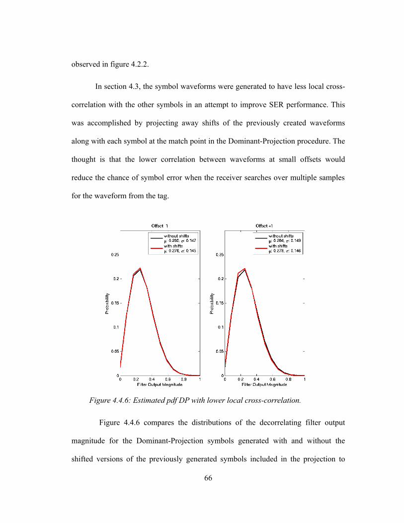
observed in figure 4.2.2.

In section 4.3, the symbol waveforms were generated to have less local cross-

correlation with the other symbols in an attempt to improve SER performance. This

was accomplished by projecting away shifts of the previously created waveforms

along with each symbol at the match point in the Dominant-Projection procedure. The

thought is that the lower correlation between waveforms at small offsets would

reduce the chance of symbol error when the receiver searches over multiple samples

for the waveform from the tag.

Figure 4.4.6: Estimated pdf DP with lower local cross-correlation.

Figure 4.4.6 compares the distributions of the decorrelating filter output

magnitude for the Dominant-Projection symbols generated with and without the

shifted versions of the previously generated symbols included in the projection to

66

generate new symbols. The distribution of the filter output for symbol 2 at +/- 1

sample delay from the synchronization point is shown with the tag transmitting

symbol 1. To improve SER performance, the lower-cross correlation should reduce

the outputs of the other three filters one sample off the match point. Here, we see that

the lower local cross-correlation only slightly reduces the mean and standard

deviation of the filter output for symbol 2. Similar results are seen for the other two

symbols.

Figure 4.4.7: Estimated pdf DP with lower local cross-correlation.

In figure 4.4.7, we see the pdfs of the transmitted waveform (symbol 1) and

the maximum of the other three waveforms with the Dominant-Projection approach

with the inclusion of the shifted communication waveforms used to achieve lower

local cross-correlation between the symbols. Here, we see that the distributions are

67

not significantly different than resulting pdfs when using symbols generated by the

original dominant projection approach, as shown in figure 4.4.3. As seen in the SER

curve in figure 4.3.3 with max=1 , the lower local cross-correlation does not

appreciably reduce the probability of symbol error.

Figure 4.4.8: Estimated pdf DP with lower local cross-correlation and average.

In figure 4.4.8, the two approaches from sections 4.2 and 4.3 are combined

such that the communication waveforms are generated with lower local cross-

correlation used with the receiver using a three sample average of the filter outputs.

Here, we see that the pdfs of the transmitted symbol and the maximum of the three

other symbols are not significantly improved by the combination of the two

approaches; therefore, a decrease in SER is not anticipated from the combining of the

68

two approaches.

4.5 MULTIPATH AND SYNCHRONIZATION

In section 3.1, multipath distortion of the radar signal between the transmitter

and the tag was considered. In the simulations, the sampled version of the multipath

distorted radar waveform was used by the tag to generate the communication

waveforms, but the symbols did not encounter a multipath channel from the tag to the

receiver. If the receiver is co-located with the transmitter, by reciprocity, the

communication signal should encounter the same multipath channel from the tag back

to the receiver. In this section, we will test the symbol error rate performance when

the communication waveforms are distorted by multipath between the tag and

receiver.

In section 3.1, it was shown that the Dominant-Projection waveform design

approach was robust to multipath distortion, generating correlated symbol waveforms

even under severe multipath conditions. For the simulations in this chapter, the

sampled radar waveform vector s is again distorted by the sampled impulse

response of the multipath profile vector h such as

s=s∗h (4.4)

where ∗ is the convolution operation. The vector s is then truncated and used by

the tag to generate the K=4 the communication waveforms ck using the

Dominant-Projection approach. The receiver again uses the undistorted sampled radar

waveform s to generate the decorrelating filters wk used to detect the symbols

69

sent by the tag. The symbol waveforms are distorted by the same multipath profile h

such that the signal sampled at the receiver r is given by

r=c k∗hS xv (4.5)

where the result of the convolution c k∗h is truncated to length NM , x is a

length 2 NM−1 vector of the radar range profile of the clutter and v is NM

samples of additive noise.

Figure 4.5.1: SER performance with and without multipath distortion from -10 dB AWGN with the receiver searching over max samples.

Figure 4.5.1 shows the SER results with the receiver searching over

max=0,1, 3,5,10 samples with and without multipath distortion of an impulse with

additive white Gaussian noise (AWGN) with an average power of -10 dB. This is the

same multipath scenario tested in section 3.1.1 with SER results (without multipath

70

between the tag and receiver) shown in figure 3.1.3. While the distortion caused by

this multipath profile did not cause different communication waveforms to be

generated between the tag and receiver (as seen by the negligible difference in SER

performance), there is a noticeable degradation in performance when the

communication waveform is distorted by this multipath profile.

Figure 4.5.2: SER performance with and without multipath distortion from from a second random impulse with the receiver searching over max

samples.

Figure 4.5.2 shows the SER results when the multipath is instead caused by a

second, randomly delayed impulse with a random complex amplitude as was used in

section 3.1.2. Again, we see an increase in symbol errors caused by the distortion of

the symbol waveform from multipath. From the SER performance of Dominant-

Projection observed in figure 3.1.4, this multipath profile did not cause enough

71

difference in the symbol waveforms to cause an increase in errors when only applied

to the radar signal between the transmitter and the tag, but does increase the

probability of error when the symbol waveforms are distorted from the tag to the

receiver.

Figure 4.5.3: SER performance with and without multipath distortion from -15 dB AWGN with the receiver searching over max samples.

Figure 4.5.3 shows the SER performance curves when the power of the

AWGN is decreased to -15 dB from the -10 dB used in the simulation shown in figure

4.5.1. Here, we see that the decrease in the power of the convolved noise decreased

the degradation caused by the multipath distortion. Also, in figure 4.5.4 we see that by

decreasing the average complex amplitude of the impulse for the second multipath

component to -7 dB from 0 dB used in figure 4.5.2, significantly decreases the

72

degradation caused by the distortion. From these plots, we see that the receiver is

robust to moderate levels of multipath distortion of the communication waveform

from the tag, but higher levels of distortion will cause an increase in the occurrence of

symbol errors. More work will need to be done to improve SER performance in the

presence of more significant multipath channel between the tag and receiver. If the

tag can determine the channel response from the incident radar waveform, the

communication waveforms could be pre-distorted such that a gain could be realized

from the multipath channel. The other possibility is the receiver using deconvolution

to remove the distortion as in adaptive pulse compression (APC) as in [17].

Figure 4.5.4: SER performance with and without multipath distortion from from a second random impulse with the receiver searching over max

samples.

73

4.6 INTERCEPT RECEIVER SYNCHRONIZATION

Lack of synchronization with the tag can also cause problems for an intercept

receiver trying to detect any communication waveforms sent. Previously, a low

probability of intercept (LPI) metric was developed to compare how well each of the

original three symbol waveform generation methods remained hidden in the clutter

and thus, had less probability of being detected by an unintended receiver. The LPI

metric was generated by projecting away a percentage of the eigenvectors of the

correlation matrix SS H and calculating the normalized correlation of the result with

the actual communication waveform sent. This LPI metric assumed both

synchronization with the tag and that the intercept receiver knew the oversample

factor M used to generate the symbol waveforms. In this section, the effect on the

LPI metric of sample offsets and a larger over sample factor for the intercept receiver

are simulated.

In simulating the delay offset's effect on the LPI metric, the symbol waveform

is shifted by the number of delay samples and added to random interference and

noise. The eigenvectors of SS H are projected away one by one with the result

correlated with the known symbol waveforms as a measure of the intercept receiver's

ability to recover the transmitted symbol waveforms. Here, only the correlation plot

of the symbol waveform sent (symbol 1) is shown to compare its LPI metric at the

different sampling offsets.

74

Figure 4.6.1: LPI Metric at different sample offsets.

In figure 4.6.1, the LPI metric is shown with the intercept receiver having

delay offsets ranging from -2 to +2 samples. Here, we see that the peak correlation

level decreases with a larger sampling offset going from about 0.30 when

synchronized to about 0.25 with +/- 2 sample offset. Also, the peak correlation level

for 0 offset is near 60% of the space projected out. At this point the normalized

correlation values with an offset are noticeably reduced. With all of this, it appears

that a lack of synchronization would make it more difficult for the intercept receiver

to detect the communication waveforms sent by the tag.

Another assumption made with the previously used LPI metric is that the

oversample factor used by the tag to generate the symbol waveforms is known by the

the intercept receiver. If this bandwidth is not known, the intercept receiver could

75

instead further oversample received waveforms while searching for the

communication waveforms. With the increased bandwidth, the symbol waveforms

must be interpolated to the oversample factor used by the simulated intercept receiver

and added to random signal and noise. The intercept receiver uses the oversampled

radar waveform to generate and project out the eigenvectors of the correlation matrix

SS H . The LPI metric is then calculated as before with the correlation of the actual

waveform sent (symbol 1) compared with the other three waveforms.

Figure 4.6.2: LPI metric with a higher sampling rate.

Figure 4.6.2 shows the LPI metric with the tag oversampling the incident

radar waveform factor of M=2 to generate the communication waveforms and the

intercept receiver using an oversample factor of M=4 to the search for the

waveforms. Here, we observe that the peak correlation level of the actual waveform

76

present is about 0.35 and for the other waveforms it is about 0.08. The increase in

peak correlation from around 0.30 seen in figure 4.6.1 may make it slightly easier for

the intercept receiver to detect the communication waveforms, but there is a higher

computational cost of using a larger bandwidth. The increase in sampling rate also

moves the normalized correlation “hump” seen in figure 4.6.1 from about 50% to

100% of the space projected away to about 25% to 75%. Based on this and the

changes in the correlation plots from sample offsets in figure 4.6.1, it may be difficult

for the intercept receiver to determine the amount of space to project away to best

detect the communication waveforms.

77

CHAPTER 5

IMPROVING WAVEFORM DESIGN

While chapters 2 and 3 dealt with issues of generating and receiving the

communication waveforms, this chapter will focus on improving the symbol

waveform design to reduce the probability of symbol error. By increasing the length

used for the incident radar waveform (and thus, increasing the communication

waveform length), each symbol should be more separable by the receiver while still

remaining hidden in the ambient scattering. Also, by generating symbol waveforms

that have less cross-correlation, they should be more separable by the receiver. If the

symbols have different amounts of correlation with the interference, mixing them

with the Hadamard Transform should equalize the correlation, leading to less errors.

Lastly, adjusting the amount of correlation of the symbol waveforms with the clutter

should influence SER performance; decreasing the correlation will increase

performance. These four methods are further explored below.

5.1 TEMPORAL EXPANSION

For each communication waveform generation method, the spectral bleeding

of the radar signal is utilized to hide the symbols for covert communication. The

bandwidth of the radar waveform is expanded as an added design dimension for the

communication waveforms such that they can remain hidden. As was seen in chapter

3, the multiple, delayed copies of the radar waveform caused by forward scattering

78

and clutter can also make it difficult to determine the length of the radar signal,

making the waveform appear longer (see figure 3.2.1). The communication

waveforms could then also be longer, while still being hidden by the ambient

scattering. Temporal expansion may then be used along with the expanded bandwidth

as an additional dimension for communication waveform design. The resulting

communication waveforms achieve an improvement in SER performance.

5.1.1 SER PERFORMANCE WITH TEMPORAL EXPANSION

In section 3.2, simulations were run with the tag determining a different length

for the radar waveform used in the generation of the communication waveforms.

From the SER results in figure 3.2.4, when the tag used a shorter length, the

probability of symbol error increased, but when a longer length was used, there was

not a significant difference in probability. It would seem that the increased SER with

the tag using a shorter waveform length would be unchanged if the receiver also used

the shorter length and if the receiver and tag both use the longer waveform length the

SER would improve. Monte Carlo simulations were then run again as in section 3.2,

but in this case both the tag and receiver use the same value N for the sampled

incident radar waveform.

The SER performance from the simulations with the tag and receiver both

using radar waveform lengths of N=100,110,130,150 used with the Dominant-

Projection approach to generate the communication waveforms is shown in figure

5.1.1. From the SER curves, we observe that the probability of symbol error is

significantly decreased with each increase in the length of the radar waveform. The

79

length could then be increased based on the ambient scattering to improve the SER

while remaining LPI.

Figure 5.1.1: SER Performance Increases with Increasing Radar Waveform Length

5.1.2 ADDED DIMENSIONALITY OF TEMPORAL EXPANSION

Increasing the length of the sampled radar waveform used in the

communication waveform generation process adds extra dimensionality for the

waveforms to occupy. Figure 5.1.2 illustrates the bandwidth and time length

expansion of the radar waveform that is used for embedding the communication

signals. Here, B and T are the notional bandwidth and time length of the

transmitted radar waveform, respectively, while B is the expanded bandwidth and

T is the expanded time length used for the communication waveforms. When the

80

correct length of the radar waveform is used, the blue section on the left side can be

used for the communication waveforms, with the red section being occupied by the

radar. By using a longer waveform, the blue section on the right can also be used as

more space for communication, but the green section is occupied by the extended

clutter of the radar and is unavailable. It appears that there would be a trade-off

between the extra bandwidth used versus the length of waveform used while

maintaining the same SER, but at least some amount of bandwidth expansion is

necessary.

Figure 5.1.2: Illustration of the expansion of time width and bandwidth of the ambient radar scattering.

5.1.3 TEMPORAL AND BANDWIDTH EXPANSION TRADE-OFF

As discussed in the last section, it appears that a trade-off can be made

between expanding the bandwidth and extending time length of the radar waveform

used in the generation of the communication waveforms while maintaining similar

SER performance. To determine the trade-off, 10,000 Monte Carlo simulations are

run for each of M=1.6,1.8,2.0,2.2,2.4 and N=100,120,140,160,180,200 . The

contour plots of iso-SER performance curves for the percentage increase in time

81

length ( T /T ) versus the percentage increase in bandwidth ( B/B ), where

T /T= N−N /N and B/B=M−1 are shown in figure 5.1.3.

Figure 5.1.3: Iso-SER contours for time width versus bandwidth expansion with -35 dB SIR and -15 dB SNR.

From the illustration in figure 5.1.2, with the blue area designating the space

available for the communication waveforms to occupy, the expected rule-of-thumb

relationship

B⋅TT =constant (5.1)

would represent the trade-off between temporal and bandwidth expansion. This

relationship is confirmed by the iso-SER contours shown in figure 5.1.3. Therefore,

given a specified value of B1/B that yields a desired symbol error rate with

T 1/T=0 , the bandwidth can be decreased to B2/B as long as the time

82

length is increased to

T 2=T [ B1B2

−1] (5.2)

to maintain similar SER performance. Since the embedded communication signal is

masked by the bleeding spectrum of the radar waveform and ambient scattering, it is

expected that reducing B/B with the required increase in T /T will be more

LPI (given that the increased time length does not extend past the length of the

ambient scattering).

5.2 SYMBOL WAVEFORMS WITH LESS CROSS-CORRELATION

The Dominant-Projection waveform generation approach produces

communication waveforms that have about -40 dB pairwise cross-correlation at the

match point. Generating communication waveforms that have lower cross-correlation

should make the symbol waveforms more separable and possibly improve SER

performance. The two methods explored are 1) giving a larger weight to the

previously generated waveforms in the projection matrix and 2) adding the Gram-

Schmitt approach.

5.2.1 WEIGHTED DOMINANT PROJECTION

With the Dominant-Projection approach, each communication waveform is

generated by projecting away the eigenvectors of the dominant space and any

previously generated waveform from a random seed vector, known to both the tag

and receiver. By giving a larger weight to the previously generated waveforms by

83

changing equation (2.6) to

Sk=[S a⋅c1 a⋅ck−1] (5.3)

where a is the weight value, they will be more prominent in the projection matrix in

equation (2.8) and the new waveform will have more of the components in common

with the other waveforms projected away. The resulting waveforms will then be less

correlated with each other.

Figure 5.2.1: Cross-correlation of codes with Weighted-Dominant-Projection.

Figure 5.2.1 shows the cross-correlation plots for each of the symbols

generated with the Weighted-Dominant-Projection approach with the first symbol

waveform. Here we see that the cross-correlation between symbols 2-4 and symbol 1

now drops to below -60 dB at the match point. This is down from the -40 dB seen

84

with the original Dominant-Projection approach shown in figure 4.3.1. The symbol

waveforms are then less correlated with the weighted symbol waveforms.

The SER performance when using the symbol waveforms generated with the

Weighted-Dominant-Projection approach is compared with the performance when

using the waveforms generated with the original Dominant-Projection approach in

figure 5.2.2. From the SER curves, we see that the symbol waveforms with less cross-

correlation generated with the Weighted-Dominant-Projection approach do not reduce

the probability of symbol error, as the SER performance with the waveforms from

both approaches is virtually identical. The reasons for this are explored more in

section 5.2.3.

Figure 5.2.2: SER performance of Dominant-Projection and Weighted Dominant-Projection.

85

5.2.2 DOMINANT-PROJECTION WITH GRAM-SCHMITT

The second method considered for generating communication waveforms that

have less cross-correlation is combining the Dominant-Projection approach with the

Gram-Schmitt procedure of producing orthonormal vectors. With the Gram-Schmitt

procedure [18], a random vector x1 is selected from the set and normalized as

u1=x1

∥x1∥(5.4)

to generate the first orthonormal vector. A second vector x2 is then selected from

the given set, the projection of x2 onto u1 is subtracted out as

u 2=x2−u1H x2u1 (5.6)

and the result is normalized as

u2=x2

∥x2∥(5.6)

to generate the second orthonormal vector. A third vector x3 is then selected from

the given set, the projection of x3 onto u1 and the projection of x3 onto u2 are

subtracted out as

u3=x3−u1H x3u1−u2

H x3u2 (5.7)

and the result again normalized to form the third orthonormal vector u3 . This can be

repeated to generate orthonormal vectors based on the size of the space that contains

the set of vectors x i .

86

Since the eigenvectors V=[v0 v1 vNM−1] of the correlation matrix SSH

used in the Dominant-Projection approach are already orthonormal, the Gram-Schmitt

procedure can then be used to generate each communication waveform as

ck=bk− ∑i=0

MN−L

bkH v ibk−∑

j=0

k−1

bkH c jbk (5.8)

where bk is the random seed vector known to both the tag and receiver, N is the

length of the radar waveform, M is the oversample factor, L is the size of the

non-dominant space and ⋅H is the Hermitian operator. Here, the dominant

eigenvectors and the previously generated symbol waveforms are directly projected

out of the seed vector.

Figure 5.2.3: Cross-correlation of symbol waveforms with Dominant-Projection with Gram-Schmitt.

87

Figure 3.2.3 shows the cross-correlation plots for the symbol waveforms

generated with the combined Dominant-Projection-Gram-Schmitt procedure. In the

plots we see that the pairwise cross-correlation is significantly reduced, dropping

down to about -160 dB for symbols 2, 3 and 4 with symbol 1.

The SER performance for these new waveforms are compared with the

original waveforms in figure 5.2.4. Here, we again see that the communication

waveforms with less cross-correlation do not appear to reduce the number of symbol

errors. Although it does not improve SER, this procedure does have the computational

benefit of only needing to perform one eigen-decomposition instead of one for each

symbol required by the Dominant-Projection approach.

Figure 5.2.4: SER performance of Dominant-Projection and Dominant-Projection with Gram-Schmitt.

88

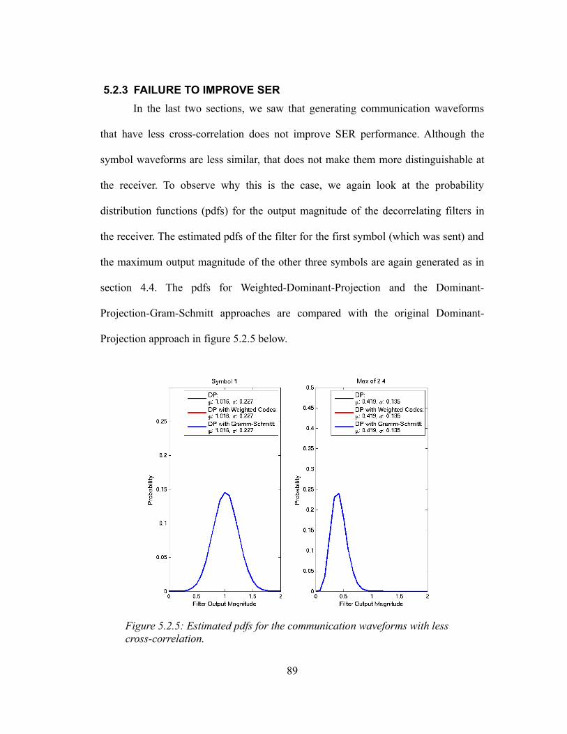
5.2.3 FAILURE TO IMPROVE SER

In the last two sections, we saw that generating communication waveforms

that have less cross-correlation does not improve SER performance. Although the

symbol waveforms are less similar, that does not make them more distinguishable at

the receiver. To observe why this is the case, we again look at the probability

distribution functions (pdfs) for the output magnitude of the decorrelating filters in

the receiver. The estimated pdfs of the filter for the first symbol (which was sent) and

the maximum output magnitude of the other three symbols are again generated as in

section 4.4. The pdfs for Weighted-Dominant-Projection and the Dominant-

Projection-Gram-Schmitt approaches are compared with the original Dominant-

Projection approach in figure 5.2.5 below.

Figure 5.2.5: Estimated pdfs for the communication waveforms with less cross-correlation.

89

From the plots, we see that both of the new approaches have basically

identical probability distributions of the filter outputs. The waveforms with less cross-

correlation do not reduce the output magnitude of the maximum of the other three

filters or increase the output magnitude of the symbol sent. From these results and the

results from section 4.4, it appears that the main contributer to the occurrence of

symbol errors is the correlation of each of the symbol waveforms with the

interference from clutter. Of course, the communication waveforms are designed to

be similar to the clutter in order to remain LPI, so the correlation is intended in the

waveform design.

5.3 EQUALIZING INTERFERENCE LEVELS AMONG SYMBOLS

Because the correlation of the communication waveforms with the

interference from ambient scattering is a major contributer to symbol error, if the

symbol waveforms each have different levels of correlation with the clutter,

interference can cause the magnitude of the decorrelating filters for symbols with a

higher correlation with the clutter to be larger on average than those with less

similarity to the clutter. This unbalance would throw off the probability distributions

causing more overlap resulting in more symbol errors.

The correlation of the symbol waveforms with the clutter interference can be

equalized by using the Hadamard Transform [19] or some other unitary

transformation. This is accomplished by taking a matrix multiplication of the symbol

waveforms with a K×K Hadamard matrix which consists of pairwise orthogonal

rows with values {−1,1} . The Hadamard Transform mixes the communication

90

waveforms in order to equalize the correlation of each waveform with the ambient

scattering, while still maintaining the pairwise orthogonality of the symbols. An

example of a 4×4 Hadamard matrix is

H 4=14 {

1 1 1 11 −1 1 −11 1 −1 −11 −1 −1 1

} . (5.9)

To simulate the effect of equalizing the correlation of the symbol waveforms

with the clutter interference by mixing them with the Hadamard Transform, we will

use a P3 waveform of length N=100 oversampled by a factor of M=2 . The size

of the non-dominant space is L=64 with K=64 communication waveforms

generated such that the entire non-dominant space is used.

The SER performance for this simulation comparing Dominant-Projection

approach with and without the Hadamard Transform is shown in figure 5.3.1. From

the plots, we observe that the Hadamard Transform does not improve the SER

performance for Dominant-Projection. The communication waveforms generated

appear to already have an equal interference with the radar clutter without the

Hadamard Transform.

91

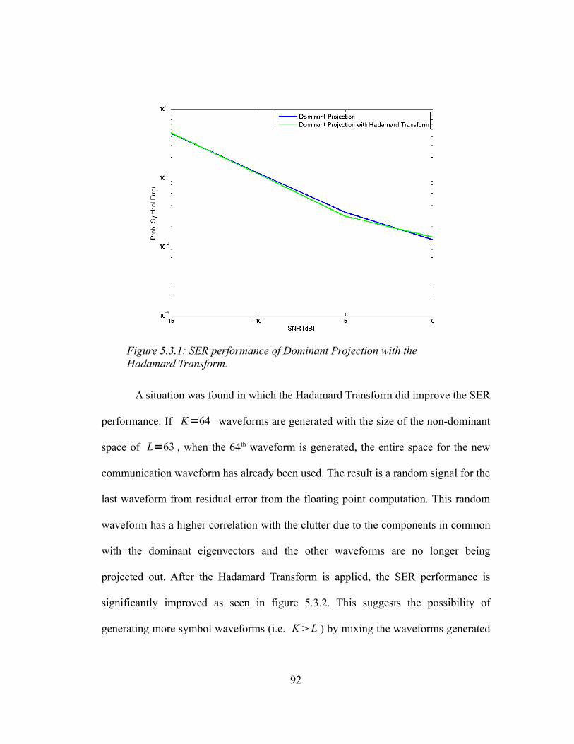
Figure 5.3.1: SER performance of Dominant Projection with the Hadamard Transform.

A situation was found in which the Hadamard Transform did improve the SER

performance. If K=64 waveforms are generated with the size of the non-dominant

space of L=63 , when the 64th waveform is generated, the entire space for the new

communication waveform has already been used. The result is a random signal for the

last waveform from residual error from the floating point computation. This random

waveform has a higher correlation with the clutter due to the components in common

with the dominant eigenvectors and the other waveforms are no longer being

projected out. After the Hadamard Transform is applied, the SER performance is

significantly improved as seen in figure 5.3.2. This suggests the possibility of

generating more symbol waveforms (i.e. KL ) by mixing the waveforms generated

92

with the Dominant-Projection approach with either random or zero vectors. It does

show that if a newly developed communication waveform generation approach yields

waveforms that have unequal correlation with the clutter, the Hadamard

Transformation could be used to equalize the interference.

Figure 5.3.2: SER performance of Dominant Projection with the Hadamard Transform equalizing a random symbol.

5.4 ADJUSTING SYMBOL CORRELATION WITH CLUTTER

The amount of correlation between the symbol waveforms and the clutter

interference can be adjusted by changing the value used for the size of the non-

dominant space L with the Dominant-Projection approach. When L is smaller,

more of the dominant eigenvectors will be projected away, making the

communication waveforms less like the ambient scattering. With a larger L , less of

93

the dominant eigenvectors will be projected out, resulting in the waveforms being

more similar to the scattering.

The SER performance for L=50,75,100,125,150 is shown above in figure

5.4.1. In the plot, we see that as expected, larger values of L have a higher

probability of symbol error and vice versa. The less similar the symbol waveforms are

to the clutter interference, the better the receiver can separate them and the less likely

an error will occur.

Figure 5.4.1: SER performance when adjusting size of nondominant space.

In figure 5.4.2, we see how the different values of L change the

distributions of the decorrelating filter outputs. With a decrease in L , the distribution

of the symbol that is present in the received waveform is narrower and taller with a

94

mean near 1. Also, the maximum of the other three filters has a mean that is reduced

with each decrease in L . Less correlation of the symbol waveforms with the ambient

scattering lessens the effect of the interference on the distributions of the

decorrelating filter output magnitude. The resulting pdfs will have less overlap

leading to the improvement in SER performance seen in figure 5.4.2.

Figure 5.4.2: Changes in estimated pdf from adjusting size of the non-dominant space.

Figure 5.4.3 shows the consequence of reducing the size used for the non-

dominant space on the ability of the communication to be covert. When the symbol

waveforms are less like the clutter, they will have a greater probability of intercept.

From the plot, it is observed that when L is decreased, the LPI metric increases.

The SER performance can then be improved by increasing the amount of the

95

dominant space that is projected out using Dominant-Projection, but improvement

comes at the cost of LPI.

Figure 5.4.3: LPI metric when adjusting the size of the dominant space.

96

CHAPTER 6

CONCLUSIONS AND FUTURE WORK

This thesis explored some of the real-world aspects of implementing intra-

pulse radar-embedded communication. Both the Eigenvectors-as-Waveforms and

Weighted-Combining communication waveform generation approaches are sensitive

to mismatches in the sampled radar waveform, since each method uses the individual,

indexed eigenvectors of the correlation of ambient scattering model generated from

the sampled waveform. Multipath distortion, sample rate differences and length

variations used for the radar waveform all cause smearing of the eigenvectors,

generating mismatched symbol waveforms and resulting in an unusable symbol error

rate. The Dominant-Projection approach, on the other hand, uses the eigenvectors of

the dominant space as a whole to generate the communication waveforms. Since the

smearing of the eigenvectors is mostly contained within the dominant and non-

dominant spaces under most of the mismatch scenarios, the approach continues to

produce symbol waveforms that are matched, making it robust to the radar waveform

mismatches. The probability of symbol error does increase, however, with a lower

sampling rate or a shorter length for the radar waveform.

Synchronization is important for intra-pulse radar embedded communication

to be effective, as the number of samples over which the receiver must look for the

communication waveform from the tag increases the probability of a symbol error.

Differing levels of synchronization could be achieved with the receiver having

97

previous knowledge of the tags location (and thus, time delay) or searching and

tracking a moving tag. SER performance would then be dependent on the receiver's

ability to track the time delay of the waveform sent by the tag.

Attempts to improve SER performance without perfect synchronization were

made by averaging over three samples and generating waveforms with lower local

cross correlation, but neither was able to reduce the number of symbol errors in

simulations. Also, communication waveforms with less cross-correlation were

generated in a failed attempt to make the symbols more separable and decrease the

chance of error. The less cross-correlated waveforms and the waveforms with less

local cross correlation do not improve SER performance due to the correlation of

each symbol with the clutter interference dominating over the pairwise cross-

correlation between each symbol waveform.

Adjustments can be made to the Dominant-Projection approach based on the

environment. Because each symbol is correlated with the ambient scattering in order

for it to be hidden and have a low probability of intercept (LPI), by projecting away

more of the dominant eigenvectors the communication waveforms will be less

correlated with the clutter interference. This will decrease the probability of symbol

error, but increase the probability of intercept. The time length of the radar waveform

can be increased in addition to the bandwidth expansion for added dimensionality in

the generation of the communication waveforms. The longer resulting symbol

waveforms are easier for the intended receiver to separate from the interference and

noise, but still remain hidden due to the extended length of the clutter interference.

98

The bandwidth used for the communication waveforms could also be decreased when

increasing the waveform length to retain the same SER performance. This trade-off

would result in more LPI communication with less bandwidth used outside the radar

as long as the longer waveform does not extend past the length of the ambient

scattering.

FUTURE WORK

1. Only the output magnitude of the decorrelating filter is used in the receiver.

The phase of the output may be used as an extra dimension to encode data (as

in M-PSK) or as a way to differentiate the signal from the noise.

2. Simulations to this point have assumed that there is always a communication

signal present. Further work is needed for detecting whether a symbol is

present in the backscatter (inclusion of the null set). The probability

distribution functions from chapter 4 could be used as a starting point for

setting a detection level, but requires calibration based on the power level of

the communication waveform at the receiver.

3. So far, only one symbol waveform has been sent by the tag at a time. With the

waveforms being orthogonal, more than one waveform could be sent by the

tag and detected at the receiver at one time, similar to CDMA or at different

dleays. Being able to send multiple waveform could be used as a way to

encode more bits for a higher data rate or to aid in detection (some number of

waveforms must be detected to determine a symbol was present).

99

4. The convolutional coding method for intra-pulse communication should be

compared with the Dominant-Projection approach in terms of symbol error

rate performance and the probability of intercept.

5. More work is needed to improve performance of the receiver when the symbol

waveforms encounter multipath distortion from the tag.

6. The tag using convolution coding may be combined with intra-pulse phase

changed to provide masking interference as well as registration for the

receiver.

7. Develop a communication waveform generation approach that is less

computationally intensive than the Dominant-Projection approach (i.e. a

method that does not require an eigen-decomposition).

100

References

[1] S.D. Blunt and P. Yatham, “Waveform design for radar-embedded

communications”, 3rd International Waveform Diversity and Design

Conference, pp. 214-218, Pisa, Italy, June 4-8, 2007.

[2] S.D. Blunt, P. Yatham, and J. Stiles, “Intra-pulse radar embedded

communications,” to appear in IEEE Trans. Aerospace & Electronic System.

[3] S.D. Blunt, J. Stiles, C. Allen, D. Deavours, and E. Perrins, "Diversity aspects

of radar-embedded communications," proc. of Intl. Conf. on Electromagnetics

in Advanced Applications, Sept. 17-21, 2007.

[4] S.D. Blunt and C.R. Biggs, “Practical Considerations for Intra-Pulse Radar-

Embedded Communications”, 4th International Waveform Diversity and

Design Conference, pp. 244-248, Orlando, FL, February 8-13, 2009.

[5] S. Kingsley and S. Quegan, Understanding Radar Systems, SciTech

Publishing, Inc., 1999.

[6] H. Stockman, “Communication by Means of Reflected Power” Proceedings

of the IRE, October 1948, pp. 1196-1204.

[7] R.M. Axline, G.R. Sloan, and R.E. Spalding, "Radar Transponder Apparatus

and Signal Processing Technique," US Patent 5,486,830, 23 Jan 1996.

[8] D. Hounam and K.H.Wagel, "A technique for the identification and

localization of SAR targets using encoding transponders," IEEE Trans.

Geoscience and Remote Sensing, vol. 39, no. 1, pp. 3-7, Jan. 2001.

[9] D.L. Richardson, S.A. Stratmoen, G.A. Bendor, H.E. Lee, and M.J. Decker,

"Tag Communication Protocol and System," US Patent 6,329,944, 11 Dec

2001.

101

[10] R.M. Axline, G.R. Sloan, and R.E. Spalding, "Transponder Data Processing

Methods and Systems," US Patent 6,577,266, 10 Jun 2003.

[11] R.C. Ormesher and R.M. Axline, "Methods and system suppressing clutter in

a gain-block, radar-responsive tag system" US Patent 7,030,805, 18 Apr 2006.

[12] J.J. Komiak, D.A. Barnum, D.E. Maron, “Digital RF tag,” US Patent

#7,106,245, issued Sept. 12, 2006.

[13] R.C.Dixon, Spread Spectrum Systems, New York: John Wiley& sons, Inc.,

1976.

[14] S. Verdu, Multiuser Detection, Cambridge University Press, Cambridge, UK,

1998.

[15] R. Lupas and S. Verdu, "Linear multiuser detectors for synchronous code-

division multiple-access channels," IEEE Trans. Information Theory, vol. 35,

pp. 123-136, Jan. 1989.

[16] B. L. Lewis and F. F. Kretschmerm, “Linear Frequency Modulation Derived

Polyphase Pulse Compression Codes”, IEEE Trans. Aerospace and Electronic

Communications, Vol AES 18, No 5, Sept 1982, pp. 637-641.

[17] S.D. Blunt and K. Gerlach, "Adaptive Pulse Compression via MMSE

Estimation," IEEE Trans. Aerospace & Electronic Systems, vol. 42, no. 2, pp.

572-584, April 2006.

[18] J. G. Proakis and Masoud Salehi, Digital Communications, Fifth Edition,

McGraw-Hill, 2008.

[19] G. L. Stüber, Principles of Mobile Communication, Second Edition, Kluwer

Academic Publishers, 2001.

102