PRACE Keynote, LinzOskar Mencer, April 2014

Computing in Space

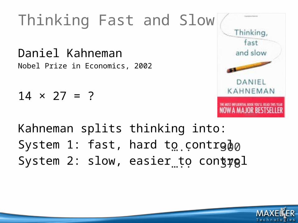
Thinking Fast and Slow

Daniel Kahneman Nobel Prize in Economics, 2002

14 × 27 = ?

Kahneman splits thinking into:System 1: fast, hard to control System 2: slow, easier to control

….. 300….. 378

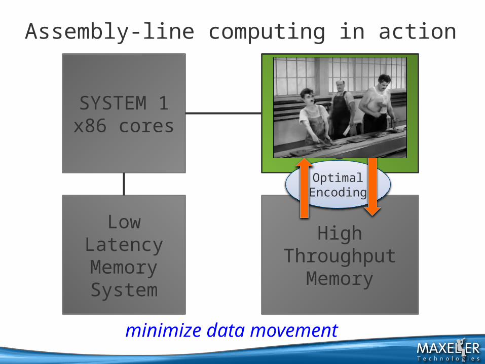
Assembly-line computing in action

SYSTEM 1x86 cores

SYSTEM 2flexible memory

plus logic

Low LatencyMemorySystem

High ThroughputMemory

minimize data movement

OptimalEncoding

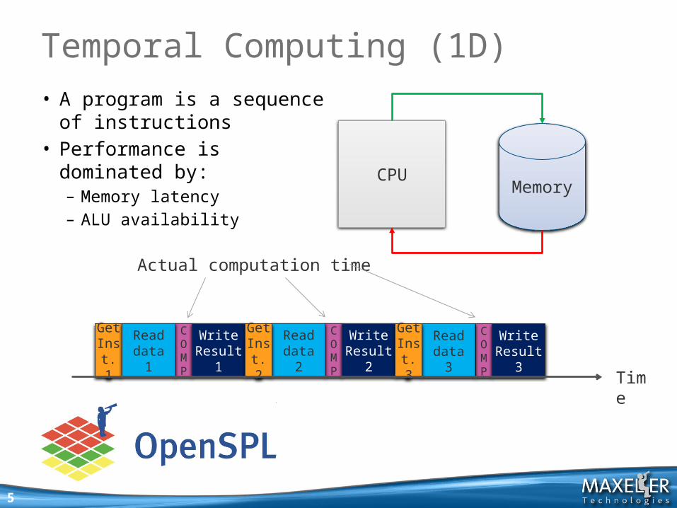
• A program is a sequence of instructions

• Performance is dominated by:– Memory latency– ALU availability

5

Temporal Computing (1D)

CPU

Time

Get Inst.

1

Memory

COMP

Read data1

Write Result

1

COMP

Read data2

Write Result

2

COMP

Read data3

Write Result

3

Actual computation time

Get Inst.

2

Get Inst.

3

6

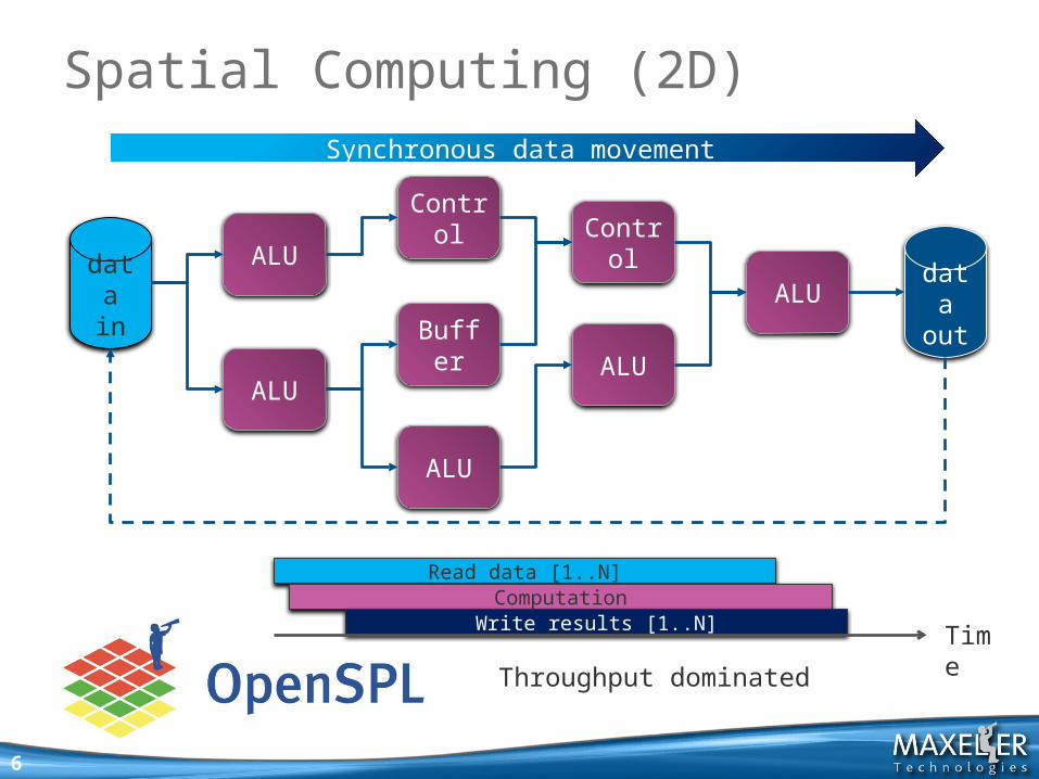
Spatial Computing (2D)

datain

ALU

ALU

Buffer

ALU

Control

ALU

Control

ALU dataout

Synchronous data movement

Time

Read data [1..N]Computation

Write results [1..N]

Throughput dominated

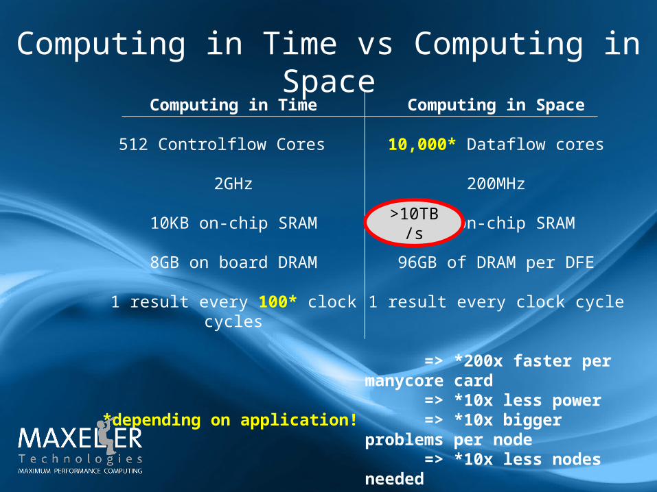
Computing in Time vs Computing in Space

Computing in Time

512 Controlflow Cores

2GHz

10KB on-chip SRAM

8GB on board DRAM

1 result every 100* clock cycles

*depending on application!

Computing in Space

10,000* Dataflow cores

200MHz

5MB on-chip SRAM

96GB of DRAM per DFE

1 result every clock cycle

=> *200x faster per manycore card

=> *10x less power => *10x bigger problems per node => *10x less nodes needed

>10TB/s

8

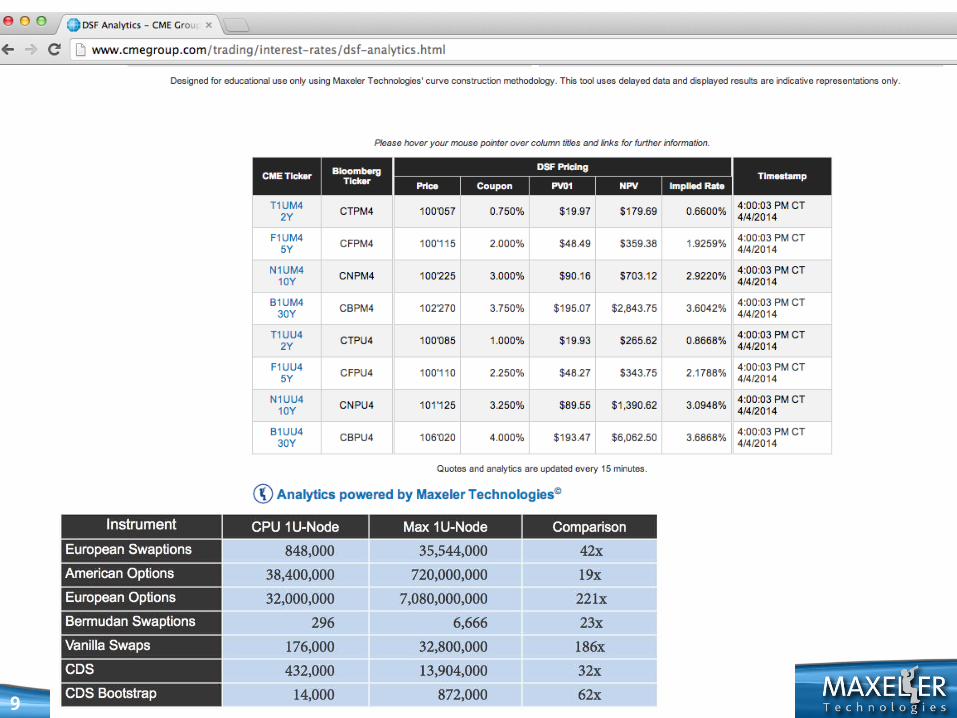
New CME Electronic Trading Gateway will be going live in March 2014!

Webinar Page: http://www.cmegroup.com/education/new-ilink-architecture-webinar.html

CME Group Inc. (Chicago Mercantile Exchange) is one of the largest options and futures exchanges. It owns and operates large derivatives and futures exchanges in Chicago, and New York City, as well as online trading platforms. It also owns the Dow Jones stock and financial indexes, and CME Clearing Services, which provides settlement and clearing of exchange trades. …. [from Wikipedia]

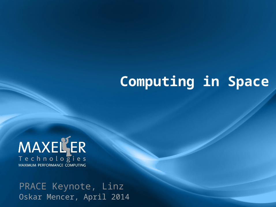
OpenSPL in Practice

9

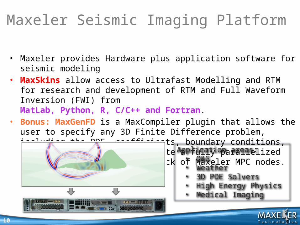
Maxeler Seismic Imaging Platform

• Maxeler provides Hardware plus application software for seismic modeling • MaxSkins allow access to Ultrafast Modelling and RTM for research and

development of RTM and Full Waveform Inversion (FWI) from MatLab, Python, R, C/C++ and Fortran.

• Bonus: MaxGenFD is a MaxCompiler plugin that allows the user to specify any 3D Finite Difference problem, including the PDE, coefficients, boundary conditions, etc, and automatically generate a fully parallelized implementation for a whole rack of Maxeler MPC nodes.

Application areas: • O&G• Weather• 3D PDE Solvers• High Energy Physics• Medical Imaging

10

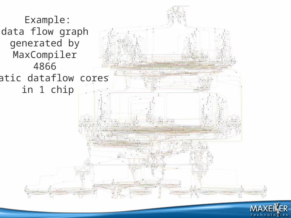
Example:data flow graph

generated by MaxCompiler

4866 static dataflow cores

in 1 chip

Mission Impossible?

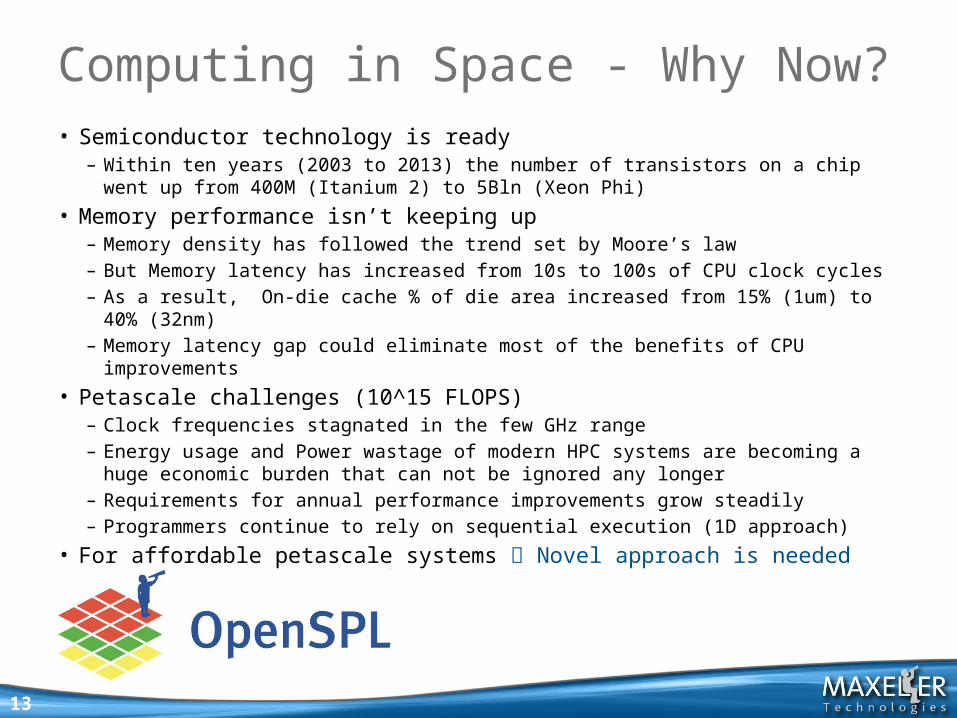
Computing in Space - Why Now?

13

• Semiconductor technology is ready– Within ten years (2003 to 2013) the number of transistors on a chip went up from

400M (Itanium 2) to 5Bln (Xeon Phi)

• Memory performance isn’t keeping up– Memory density has followed the trend set by Moore’s law– But Memory latency has increased from 10s to 100s of CPU clock cycles– As a result, On-die cache % of die area increased from 15% (1um) to 40% (32nm) – Memory latency gap could eliminate most of the benefits of CPU improvements

• Petascale challenges (10^15 FLOPS)– Clock frequencies stagnated in the few GHz range– Energy usage and Power wastage of modern HPC systems are becoming a huge

economic burden that can not be ignored any longer– Requirements for annual performance improvements grow steadily – Programmers continue to rely on sequential execution (1D approach)

• For affordable petascale systems Novel approach is needed

x

x

+

30

y

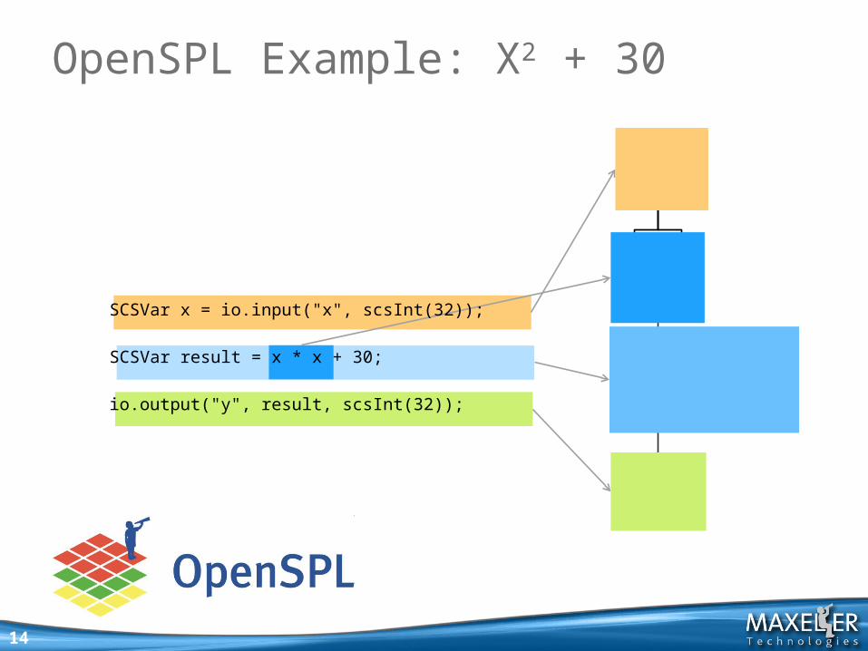
SCSVar x = io.input("x", scsInt(32));

SCSVar result = x * x + 30;

io.output("y", result, scsInt(32));

14

OpenSPL Example: X2 + 30

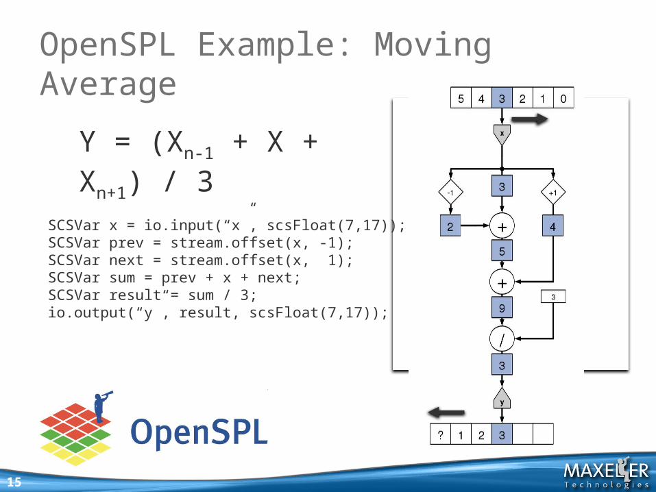
OpenSPL Example: Moving Average

15

SCSVar x = io.input(“x”, scsFloat(7,17));SCSVar prev = stream.offset(x, -1);SCSVar next = stream.offset(x, 1); SCSVar sum = prev + x + next; SCSVar result = sum / 3;io.output(“y”, result, scsFloat(7,17));

Y = (Xn-1 + X + Xn+1) / 3

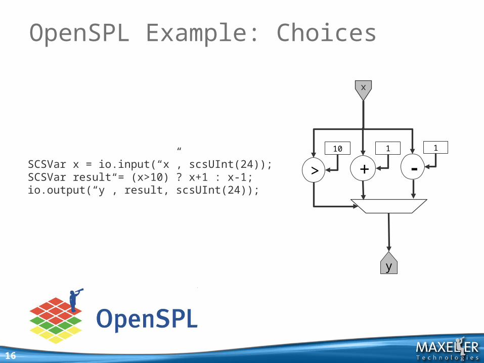
OpenSPL Example: Choices

16

x

+1

y

-1

>

10

SCSVar x = io.input(“x”, scsUInt(24));SCSVar result = (x>10) ? x+1 : x-1;io.output(“y”, result, scsUInt(24));

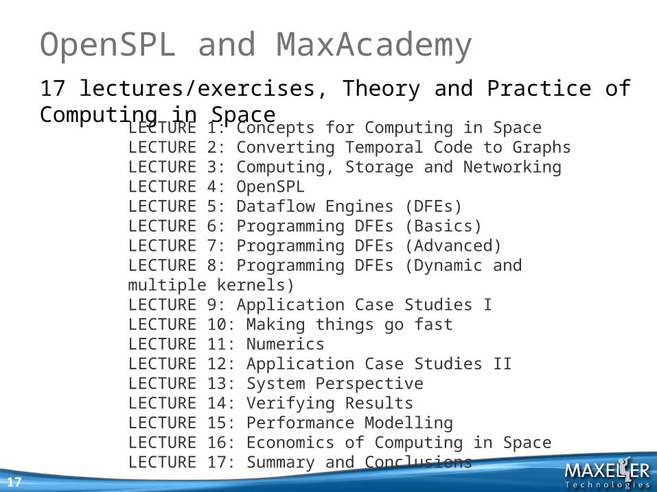
17 lectures/exercises, Theory and Practice of Computing in Space

17

OpenSPL and MaxAcademy

LECTURE 1: Concepts for Computing in SpaceLECTURE 2: Converting Temporal Code to GraphsLECTURE 3: Computing, Storage and NetworkingLECTURE 4: OpenSPLLECTURE 5: Dataflow Engines (DFEs) LECTURE 6: Programming DFEs (Basics)LECTURE 7: Programming DFEs (Advanced)LECTURE 8: Programming DFEs (Dynamic and multiple kernels)LECTURE 9: Application Case Studies ILECTURE 10: Making things go fastLECTURE 11: NumericsLECTURE 12: Application Case Studies IILECTURE 13: System Perspective LECTURE 14: Verifying ResultsLECTURE 15: Performance ModellingLECTURE 16: Economics of Computing in SpaceLECTURE 17: Summary and Conclusions

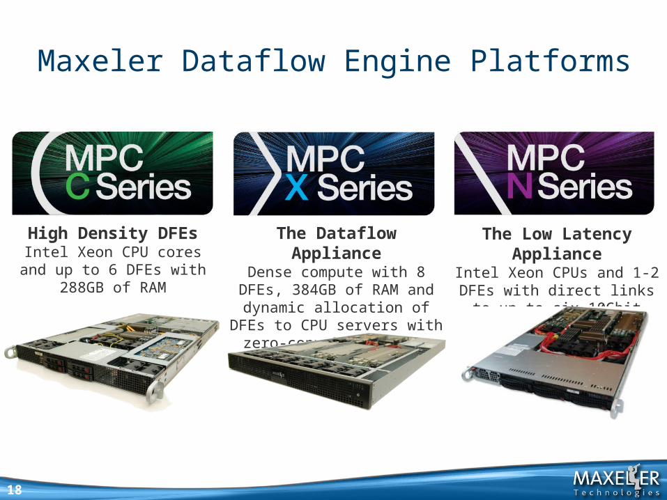
Maxeler Dataflow Engine Platforms

18

High Density DFEsIntel Xeon CPU cores and up to 6

DFEs with 288GB of RAM

The Dataflow ApplianceDense compute with 8 DFEs, 384GB of RAM and dynamic

allocation of DFEs to CPU servers with zero-copy RDMA access

The Low Latency ApplianceIntel Xeon CPUs and 1-2 DFEs with

direct links to up to six 10Gbit Ethernet connections

19

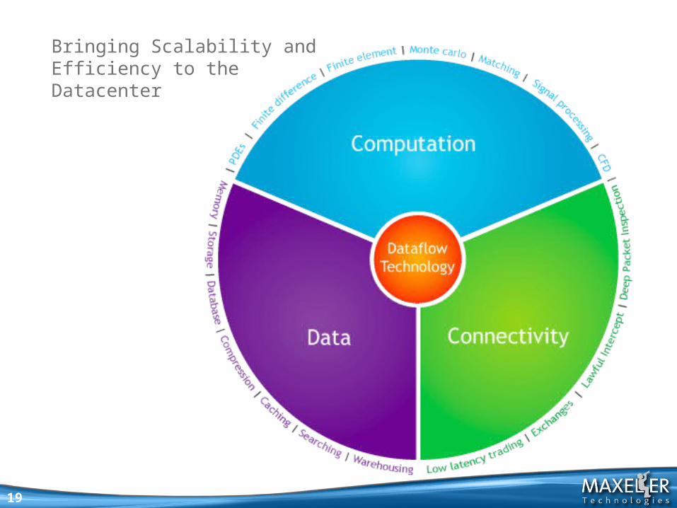
Bringing Scalability andEfficiency to theDatacenter

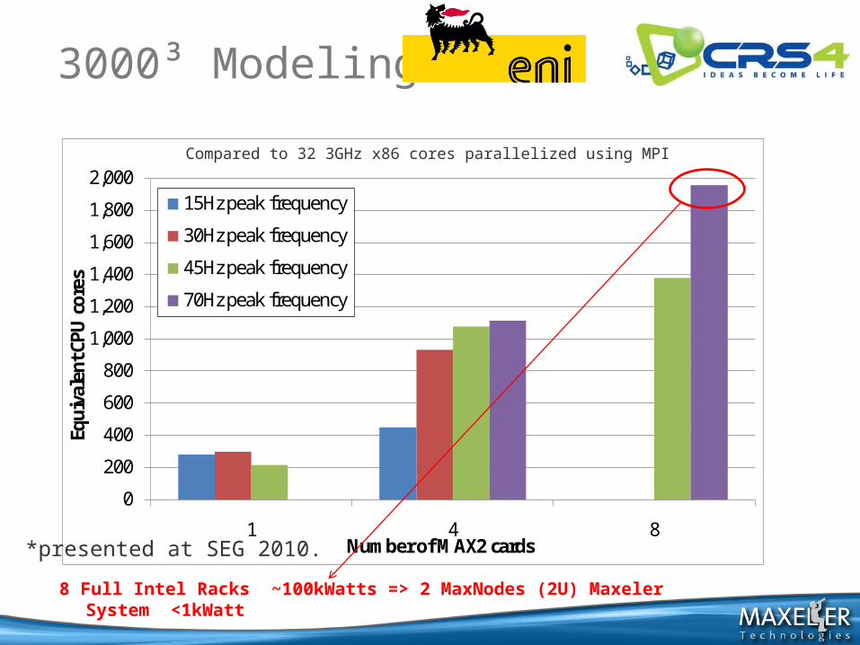
3000³ Modeling

0

200

400

600

800

1,000

1,200

1,400

1,600

1,800

2,000

1 4 8

Equi

vale

nt C

PU c

ores

Number of MAX2 cards

15Hz peak frequency

30Hz peak frequency

45Hz peak frequency

70Hz peak frequency

*presented at SEG 2010.

Compared to 32 3GHz x86 cores parallelized using MPI

8 Full Intel Racks ~100kWatts => 2 MaxNodes (2U) Maxeler System <1kWatt

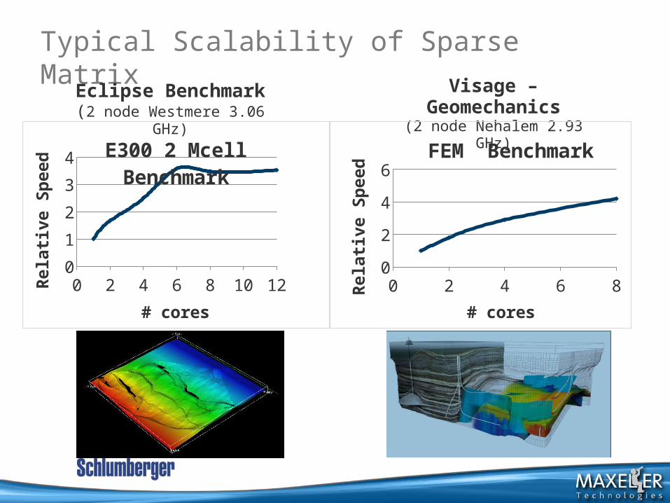
Typical Scalability of Sparse MatrixVisage –

Geomechanics(2 node Nehalem 2.93 GHz)

Eclipse Benchmark(2 node Westmere 3.06 GHz)

0 2 4 6 8 10 120

1

2

3

4E300 2 Mcell Benchmark

# cores

Rela

tive

Spee

d

0 2 4 6 8012345

FEM Benchmark

# cores

Rela

tive

Spee

d

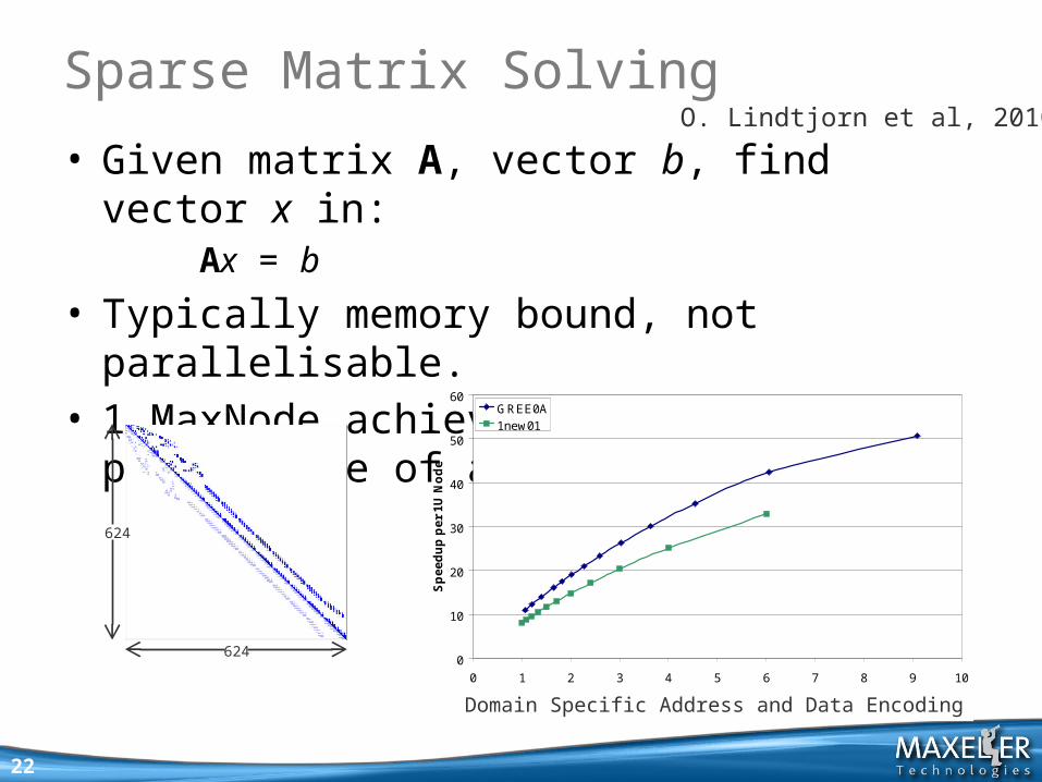
• Given matrix A, vector b, find vector x in:Ax = b

• Typically memory bound, not parallelisable.• 1 MaxNode achieved 20-40x the performance of an

x86 node.

22

Sparse Matrix SolvingO. Lindtjorn et al, 2010

624

624 0

10

20

30

40

50

60

0 1 2 3 4 5 6 7 8 9 10

Compression Ratio

Sp

ee

du

p p

er

1U

No

de

GREE0A1new01

Domain Specific Address and Data Encoding

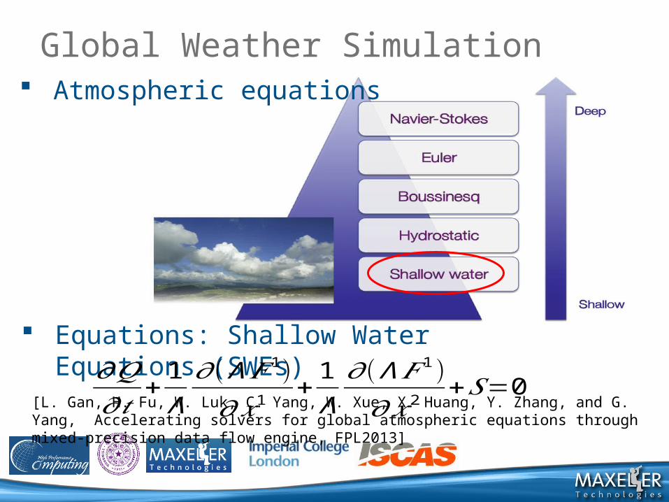
Equations: Shallow Water Equations (SWEs)

Atmospheric equations

𝜕𝑄𝜕𝑡

+ 1Λ𝜕(Λ 𝐹 1)𝜕 𝑥1 + 1

Λ𝜕(Λ 𝐹1)𝜕 𝑥2 +𝑆=0

Global Weather Simulation

[L. Gan, H. Fu, W. Luk, C. Yang, W. Xue, X. Huang, Y. Zhang, and G. Yang, Accelerating solvers for global atmospheric equations through mixed-precision data flow engine, FPL2013]

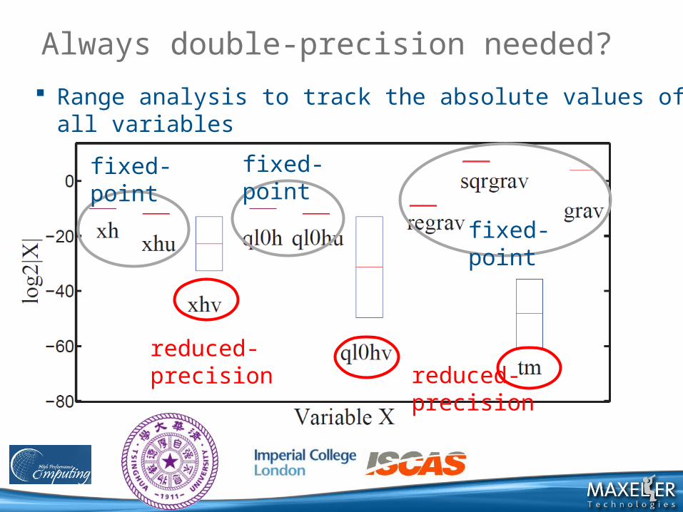
Always double-precision needed? Range analysis to track the absolute values of all variables

fixed-point fixed-point

fixed-point

reduced-precisionreduced-precision

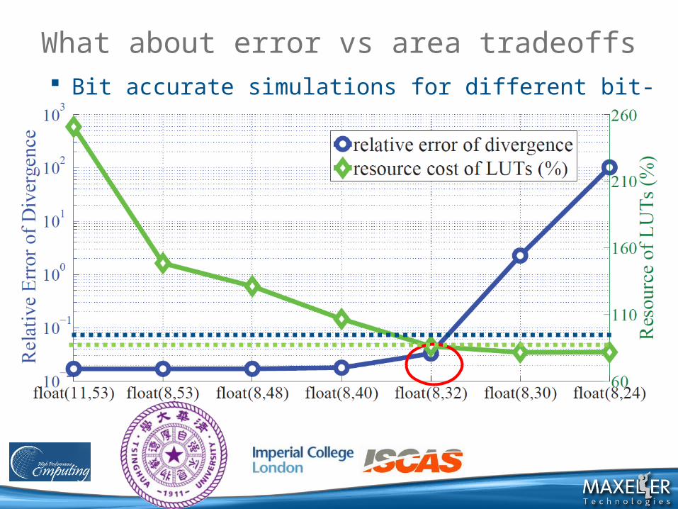
What about error vs area tradeoffs Bit accurate simulations for different bit-width configurations.

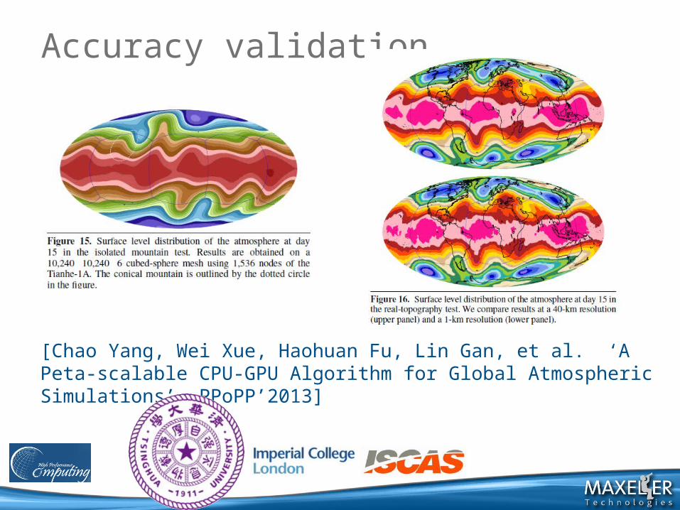
Accuracy validation

[Chao Yang, Wei Xue, Haohuan Fu, Lin Gan, et al. ‘A Peta-scalable CPU-GPU Algorithm for Global Atmospheric Simulations’, PPoPP’2013]

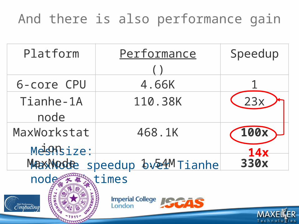
And there is also performance gain

Meshsize: MaxNode speedup over Tianhe node: 14 times

Platform Performance()

Speedup

6-core CPU 4.66K 1

Tianhe-1A node 110.38K 23x

MaxWorkstation 468.1K 100x

MaxNode 1.54M 330x

14x

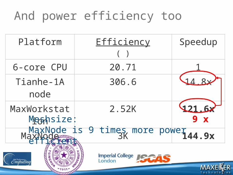
And power efficiency too

Platform Efficiency( )

Speedup

6-core CPU 20.71 1Tianhe-1A node 306.6 14.8xMaxWorkstation 2.52K 121.6x

MaxNode 3K 144.9x

Meshsize: MaxNode is 9 times more power efficient

9 x

29

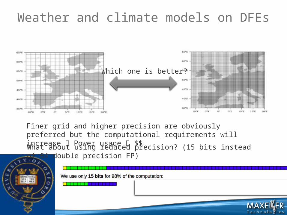
Weather and climate models on DFEs

Which one is better?

Finer grid and higher precision are obviously preferred but the computational requirements will increase Power usage $$

What about using reduced precision? (15 bits instead of 64 double precision FP)

30

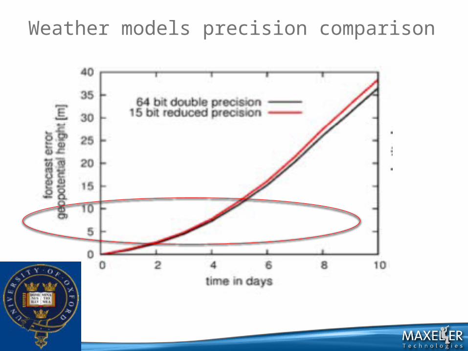
Weather models precision comparison

31

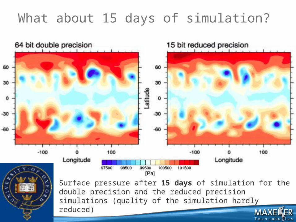
What about 15 days of simulation?

Surface pressure after 15 days of simulation for the double precision and the reduced precision simulations (quality of the simulation hardly reduced)

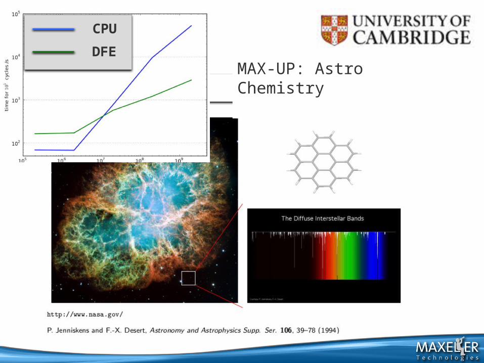
MAX-UP: Astro Chemistry

CPU

DFE

33

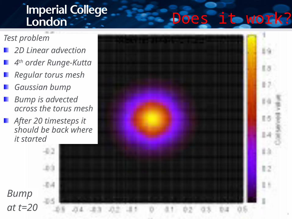
Does it work?Test problem

2D Linear advection

4th order Runge-Kutta

Regular torus mesh

Gaussian bump

Bump is advected across the torus mesh

After 20 timesteps it should be back where it started

Bump

at t=20

34

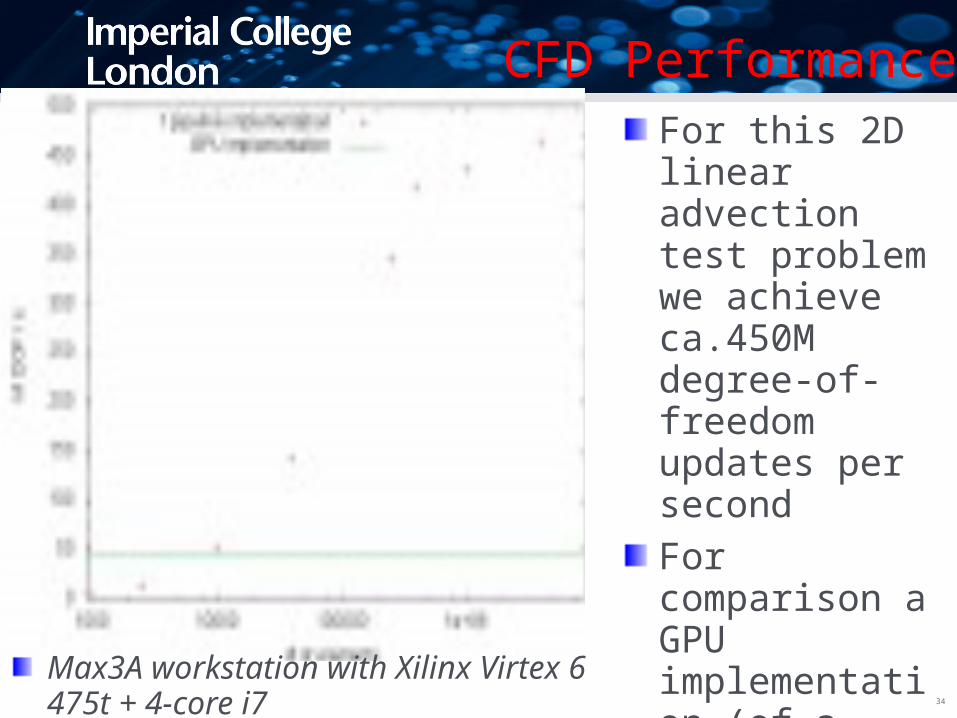
CFD PerformanceFor this 2D linear advection test problem we achieve ca.450M degree-of-freedom updates per second

For comparison a GPU implementation (of a Navier-Stokes solver) achieves ca.50M DOFs/s

Max3A workstation with Xilinx Virtex 6 475t + 4-core i7

35

CFD Conclusions

You really can do unstructured meshes on a dataflow accelerator

You really can max out the DRAM bandwidth

You really can get exciting performance

You have to work pretty hard

Or build on the work of others

This was not an acceleration project

We designed a generic architecture for a family of problems

37

We’re Hiring

Candidate Profiles

Acceleration Architect (UK)Application Engineer (USA)System Administrator (UK)Senior PCB Designer (UK)Hardware Engineer (UK)

Networking Engineer (UK)Electronics Technician (UK)