Drexel UniversityMechanical Engineering Department

A Senior Design Proposal Titled:

Binary Refrigerant Refrigerator

Project 25

MEM491

Samuel BeccariaAbhinav DuggalMathew Smith

Xiaoyi Zhu

November 24, 2014Advisory: Bakthier Farouk

1

Abstract

The objective of the project is to design, build and test an optimized domestic vapor compression refrigerator that uses a binary refrigerant mixture instead of the more traditional single component refrigerant refrigerators. The temperature glide effect (a range of saturation temperature for a specific saturation pressure) allows for temperature changes during the constant pressure boiling, which occurs in binary refrigerant refrigeration cycles. This changing temperature offers potential energy/efficiency advantages for household refrigeration, because they typically have two different evaporator temperatures for the fridge and freezer. Optimization algorithms will be implemented to choose the specific combination of the mixture components for maximizing the COP of the refrigeration system. Stakeholders for this project include consumers, as well as appliance manufacturers and the environment, because the refrigerant mixture conserves energy while also reducing harmful emissions. The refrigerants for the binary system are selected based on review and using analytical data to generate concentration plots and calculate the temperature glide for different combinations. Based on the analytical data developed in MATLAB, experimental tests will be performed with various refrigerant concentrations in a real household refrigerator/freezer, and the required energy will be measured to determine the mass fractions that produce the highest COP. The experimental procedure will entail a refrigerator that has been charged with the selected refrigerant mixture which will be run with thermocouples placed on the inside. Once the temperature and energy data is collected, the COP will be calculated from those values and compared with the analytical COP results.

2

Table of ContentsAbstract.......................................................................................................................................................2

1. Introduction.........................................................................................................................................4

1.1. Background................................................................................................................................4

1.2. Stakeholders and Needs.............................................................................................................5

1.3. Problem Statement....................................................................................................................5

2. Methods...............................................................................................................................................6

2.1. Reverse Rankine Cycle..............................................................................................................6

2.2. Thermophysical Properties of Binary Mixtures......................................................................6

2.3. Optimization Methods...............................................................................................................7

2.3.1. Objective Function.............................................................................................................7

2.3.2. Constraint Equations.........................................................................................................7

3. Design Description..............................................................................................................................8

3.1. Sliding Temperatures................................................................................................................8

3.2. Refrigeration Systems................................................................................................................8

3.3. Experimental Design and Construction of Binary Refrigerant System.................................8

4. Context and Impacts..........................................................................................................................10

4.1. Economic Analysis...................................................................................................................10

4.2. Environmental Impact Analysis.............................................................................................10

4.3. Social Impact Analysis.............................................................................................................10

4.4. Ethical Analysis........................................................................................................................11

5. Project Management..........................................................................................................................11

5.1. Team Organization..................................................................................................................11

5.2. Schedule and Milestones..........................................................................................................11

5.2.1. Fall Term: Proposal Preparation....................................................................................11

5.2.2. Winter Term: Optimized System Development.............................................................11

5.2.3. Spring Term: Testing and Data Collection....................................................................12

5.3. Project Budget..........................................................................................................................12

4 Thermocouples Garland 4518817...........................................................................................................12

Power Meter Energy Monitor....................................................................................................................12

Total..........................................................................................................................................................12

6. Discussions and Alternative Concepts...............................................................................................12

6.1. Binary Refrigerant Selection...................................................................................................12

3

6.1.1. Alternative to Binary Refrigerant Mixture........................................................................13

6.2. Thermodynamic System Selection..........................................................................................13

6.2.1. Alternative to Refrigeration System...................................................................................13

6.3. Mathematical Modeling with MATLAB................................................................................14

6.3.1. Alternative to Optimization Process...................................................................................14

7. Summary and Conclusion..................................................................................................................14

7.1. Optimized Design.....................................................................................................................14

7.2. Construction of Experimental Apparatus..............................................................................14

7.3. Testing of Experimental Apparatus.......................................................................................14

8. Proposed Task...................................................................................................................................14

9. References.........................................................................................................................................15

10. Appendices....................................................................................................................................17

10.1. Appendix A: Supplementary Material to Methods...........................................................17

10.2. Appendix B: Analysis of Lorenz-Meutzner Cycle.............................................................19

10.3. Appendix C: Isentropic Work of Compressor and Related MATLab code....................20

10.4. Appendix D: Justification of Refrigerant Mixture Tables................................................26

4

1. Introduction1.1. BackgroundRefrigerators that currently exist in the home employ a single refrigerant as the working fluid. The working fluid through a refrigerator has to meet a certain set of safety and thermophysical requirements. The best refrigerant to use would have low toxicity, low flammability, a high heat of vaporization, a small specific heat and specific volume and low ozone depletion and global warming potentials. Unfortunately single refrigerants are often very friendly to the environment but have very poor thermophysical properties, or have excellent thermophysical properties but have a high potential to harm the environment. There is a work around to this by the use of a binary refrigerant [2].

A binary refrigerant experiences one or two states, liquid, vapor or liquid-vapor, dependent upon the pressure and temperature of the system and the saturation pressure of the refrigerants in mixture. In most cases this allows for a temperature glide effect (a range of saturation temperature for a given saturation pressure) that allows the freezer temperature to be reached at a much lower pressure [14]. Additionally, by mixing refrigerants with varying pros and cons, i.e. mixing a refrigerant with poor thermophysical properties that does little harm to the environment and refrigerant with excellent thermophysical properties that does a lot of harm to the environment, the harm to the environment can be minimized while still seeing gains in the COP [15].

Currently, refrigerators use a single refrigerant as their working fluid called HFC-134a (1,1,1,2-Tetrafluoroethane), which does not deplete the ozone layer and has good thermophysical properties. However R134a has high GWP (global warming potential) of 1300. The Kyoto Protocol of the United Nations Framework Convention on Climate Change (UNFCCC) calls for reductions in emissions of six categories of greenhouse gases, including hydrofluorocarbons (HFCs) used as refrigerants. From the environmental, economic, social and ethical aspects, it is urgent to find a good alternative option for HFC refrigerant [21].

Household refrigerators are identified as the most energy consuming appliance of all household appliances. It has been proposed that a mixture of refrigerants can offset the energy consumption of household refrigerators while providing an environmentally friendly alternative to HFC-134a. The reason for using binary refrigerants is that binary refrigerants can be tailored to meet a specific temperature requirement, -18°C in the freezer, while simultaneously lowering the power output to reach that temperature. It is also possible to control the properties such as toxicity, flammability, oil miscibility by manipulating the composition. Most importantly, using a binary mixture as the working fluid increases the COP of the system, allowing for greater energy efficiency [21].

1.2. Stakeholders and NeedsThe stakeholders of this project include homeowners, supermarkets, facility owners and vendors. Their needs must be considered and implemented into the design of the binary refrigerant to create a successful product.

5

Once the binary refrigerant mixture has been found through optimization and testing methods, homeowners can use the binary refrigerants in their household refrigerators, which can improve the energy efficient thus saving the money. The same applies to other stakeholders.

1.3. Problem StatementThe objective of the project is to design, build and test a domestic vapor compression refrigerator that uses a binary refrigerant mixture instead of the more traditional single component refrigerant refrigerators.

2. MethodsThe optimization of the binary refrigerant system will yield an optimized design that will be used in the building and testing phase of this project. With the optimization algorithm, made in MATLAB, the optimal mixture of refrigerants that yield the maximum COP of the system will be found. Thus the completion of this project rests upon the understanding of refrigeration systems, the thermodynamic properties of mixtures and how the working fluid behaves within a refrigeration system. This understanding will be established analytically in order to use the optimization algorithm. Once the refrigeration system is represented analytically, the optimization algorithm, in this case the method of Lagrange multipliers, will be used to generate the optimized design of the refrigerant mixtures that yields the maximum COP. The optimization of the refrigerant mixtures that yield the maximum COP will be done via simulation in MATLAB.

2.1. Reverse Rankine CycleThe refrigeration system can be modeled as a simple vapor-compression cycle. The vapor-compression cycle, or the Reverse Rankine cycle, consists of four components, a compressor, condenser, throttling valve and evaporator. The states 1, 2, 3 and 4, are the evaporator outlet, compressor outlet, condenser outlet and throttling valve outlet respectively. The entirety of this process for a single refrigerant can be shown in the T-s diagram in Figure 4 in Appendix A [23].

The compression process is assumed to be adiabatic and isentropic. The working fluid enters the compressor from state 1 as a saturated vapor and leaves the compressor in state 2 as a superheated vapor. From state 2 the working fluid enters the condenser, where it is condensed from a superheated vapor to saturated liquid in state 3. The saturated liquid in state 3 enters the throttling valve where the saturated liquid is turned into a saturated liquid-vapor mixture of quality, x in state 4. The working fluid from state 4 feeds into the evaporator, where the temperature of the working fluid is constant through the evaporator and the saturated liquid-vapor mixture is returned to a saturated vapor at state 1 [23].

Another important factor to note is that the pressure is constant over the evaporator and the condenser. If the pressures are known for each, then the temperatures at state 3, state 4 and state 1 can be found. As well, since the compression process from state 1 to state 2 is isentropic, if the entropy at state 1 is known then the temperature of the superheated vapor can be found. Having these concepts in mind allows for the setup of the analysis of this system to maximize for the COP [19],[20],[23].

6

2.2. Thermophysical Properties of Binary MixturesThe equations of states of the system become more complex when a binary refrigerant mixture is used as the working fluid. To grasp this concept the properties of a binary mixture of any two fluids must be explored. A binary refrigerant is a refrigerant that is a mixture of two refrigerants. The thermophysical properties of a binary mixture of fluids are dependent upon the refrigerants saturation temperatures and pressures [6]. If the saturation temperatures or pressures of two fluids are similar then the mixture will be azeotropic. This means that the fluids behave as if they were one fluid when undergoing changes in state from saturated vapor to saturated liquid and vice versa. However if the two fluids vary widely in their saturation temperatures or pressures, this will result in a zeotropic mixture. A zeotropic mixture experiences a dome, where at certain temperatures the mixture will be a combination of liquid and vapor of each component.

To illustrate the difference between azeotropic and zeotropic mixtures, Figures 5 and 6 in Appendix A demonstrate the vapor-liquid equilibrium graphs of a binary mixture of refrigerants, R143A/R125 and R152A/R125 respectively.

2.3. Optimization MethodsFinally, given the thermal system and the working fluid, the Lagrange multiplier method will be utilized in the optimization process. The optimization process outputs the refrigerant mixture that, when run through the cycle, will produce the maximum COP.

The Lagrange multiplier method is a mathematical model to solve a system of linear or nonlinear equations simultaneously. The main components of the method are detailed in Appendix A.

2.3.1. Objective FunctionIn order to optimize the refrigerant mixture that gives the optimal design COP the Lagrange multiplier method is used by finding an objective function. The objective function to be optimized, in this case the COP as a function of temperature, mass flow rate, and the refrigeration load, must be created, and is shown in EQ 1.

COP=Ql

mc (1−T 1

T 2)

(1)

Where c is a constant, m is the mass flow rate, Ql is the heat taken in by the working fluid through the evaporator, and T1 and T2 are the temperatures at states 1 and 2 respectively. Ql is a given property based off of the type of refrigerator and the constant c can be found using the method in Appendix C.

2.3.2. Constraint EquationsAn additional part to deriving the optimal design requires a set of constraint equations to be made. The constraint equations represent physical aspects of the system that restrict the relationship between the variables in the objective function to a specific value. The relations that are made in the constraint equations are often derived from the actual system to be optimized. However to avoid having a system that is overly constrained the number of constraint equations should be less than the number of variables in the objective function. Additionally between the constraint equations every variable in the objective

7

function should be represented. The set of constraint equations for the system to be optimized can be represented in EQ. 2.

ϕ1=f ( x1 , x2, …, xn )=0⋮ϕm=f ( x1 , x2 ,… , xn )=0(2)

Where ϕ is the constraint equation that the objective function is subject to, n is the number of variables in the objective function and m is the number of constraint equations. It is important to note that m < n. The rest of the optimization procedure to achieve the optimal design is detailed in Appendix A.

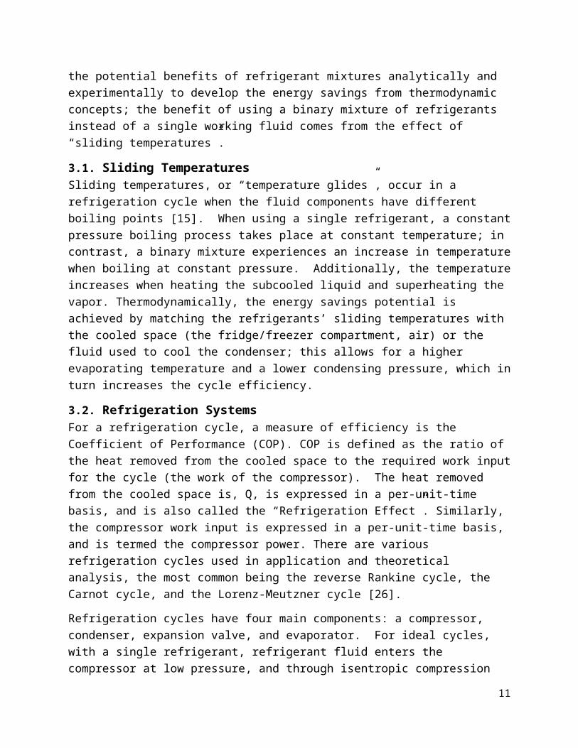
3. Design DescriptionThe aim of this project is to design, build and test an optimized domestic vapor compression refrigerator that uses a binary refrigerant mixture instead of the more traditional single component refrigerant refrigerators. The concept for this project came from several papers by Wilbert F. Stoecker, who investigated the potential benefits of refrigerant mixtures analytically and experimentally to develop the energy savings from thermodynamic concepts; the benefit of using a binary mixture of refrigerants instead of a single working fluid comes from the effect of “sliding temperatures”.

3.1. Sliding TemperaturesSliding temperatures, or “temperature glides”, occur in a refrigeration cycle when the fluid components have different boiling points [15]. When using a single refrigerant, a constant pressure boiling process takes place at constant temperature; in contrast, a binary mixture experiences an increase in temperature when boiling at constant pressure. Additionally, the temperature increases when heating the subcooled liquid and superheating the vapor. Thermodynamically, the energy savings potential is achieved by matching the refrigerants’ sliding temperatures with the cooled space (the fridge/freezer compartment, air) or the fluid used to cool the condenser; this allows for a higher evaporating temperature and a lower condensing pressure, which in turn increases the cycle efficiency.

3.2. Refrigeration SystemsFor a refrigeration cycle, a measure of efficiency is the Coefficient of Performance (COP). COP is defined as the ratio of the heat removed from the cooled space to the required work input for the cycle (the work of the compressor). The heat removed from the cooled space is, Q, is expressed in a per-unit-time basis, and is also called the “Refrigeration Effect”. Similarly, the compressor work input is expressed in a per-unit-time basis, and is termed the compressor power. There are various refrigeration cycles used in application and theoretical analysis, the most common being the reverse Rankine cycle, the Carnot cycle, and the Lorenz-Meutzner cycle [26].

Refrigeration cycles have four main components: a compressor, condenser, expansion valve, and evaporator. For ideal cycles, with a single refrigerant, refrigerant fluid enters the compressor at low pressure, and through isentropic compression (no change in entropy), the compressor’s power/work input raises the pressure of the refrigerant [26]. Compression produces superheated vapor, which enters the condenser and loses heat to the condenser cooling fluid (often water or surrounding air) at constant pressure. This heat loss cools the refrigerant producing saturated

8

liquid. From here the refrigerant enters an expansion valve, which lowers the pressure of the refrigerant. The refrigerant flows to the evaporator, which is where the refrigeration effect occurs; the higher temperature cooling space passes heat to the refrigerant, in turn raising the refrigerant temperature and cooling the fridge/freezer compartment [21],[26].

3.3. Experimental Design and Construction of Binary Refrigerant SystemThe binary refrigerant system that will be constructed for experimental purposes will simply be a modified refrigerator outfitted with thermocouples and a power sensor. When purchased, the refrigerator will be discharged of its current working fluid and the refrigerator will be recharged with the optimized binary mixture. The refrigerator shown in Figure 1 will be used for the experimentation.

Figure 1. The Igloo 1.7-cu ft Refrigerator

The refrigerator system can be represented in Figure 2.

Figure 2. The thermodynamic system representing the refrigerator system

And finally the refrigerator system with the additional sensors is shown in Figure 3.

9

Figure 3. The refrigeration system with added thermocouples and power sensors

This refrigerator will be modified with the thermocouples and charged with the refrigerant mixture in the winter term of this year.

4. Context and Impacts4.1. Economic AnalysisFor the household refrigerators, the daily energy value is about 1400 watt-hours/day. The electricity usage of refrigerator is inconspicuous in people's minds, but because refrigerators work year-round ever since the moment it gets home, and then hardly unplug the power, therefore it is actually the greatest power consumption of ordinary household appliances. Therefore, in order to reduce the power consumption of the family throughout the year, choose binary refrigerants refrigerator is probably the most obvious effect. It can help the family save some money on the household refrigerators.

4.2. Environmental Impact AnalysisSince environment friendly become more and more important in nowadays society, environmental impact is the one of the major concern of the product. If the choice of binary refrigerants is widely used in the worldwide instead of R134, it is very helpful for the global warming problem since 134a has high GWP of 1300, and the chosen binary refrigerants has much lower global warming potential. Even using of these binary refrigerants can’t change greenhouse phenomenon, it can slow the greenhouse effect and it is very environment friendly. [2]

4.3. Social Impact AnalysisThe products might only save not much electricity in one family, but it have the potential to save large amounts of electricity for society. In areas with less access to electricity these applications may potentially help a lot of people. For the developing country like China, some places are

10

really well developed but some places not. They have very large gap in wealth, some places even don’t access of the electricity, using the products will help a lot of this situation. And for the developed country like America, using the product can save the energy consumption for the country as well as much money, which can be used in other fields.

4.4. Ethical AnalysisThe products complies with ethical codes. The products are low cost and will be affordable by all the ordinary people. The product will not give any person or party any significant power to take advantage of or abuse other parties. There are still many developing country lacking of electricity, the product will helps. And it is environment friendly, most importantly, it is safe, it has no harm to the people.

5. Project Management5.1. Team OrganizationWeekly meetings were held with the team’s advisor Dr. Farouk on Wednesdays at 11am in the Randell building. During these meetings the group was able to fill Dr. Farouk in on weekly progress and also update Dr. Farouk with any questions, comments, and concerns that may have developed in the past week. Then Dr. Farouk assigned weekly tasks for the group or for individuals in the group. Weekly team meetings amongst the individuals were set to work together on the weekly tasks Dr. Farouk assigned.

The group has four members. One member will be held accountable for scheduling meetings, keeping meeting minutes, and keeping track of project deadlines and requirements. The group use Google drive to store all the work data and research papers and the meeting minutes. Google drive allows each member of the team to access and edit files

5.2. Schedule and Milestones5.2.1. Fall Term: Proposal PreparationIn the fall term, the group is mainly focus on the research aspects of the project, the group found and read a multitude of research papers from engineering village and also from other sources. The research papers pertained to binary refrigerants and offered insight into their thermophysical properties and how they behave in various compression cycles. The group learned about the Newton-Raphson method, and how to use MATLAB to build the functioning code to solve a specific optimization problem. The boiling point diagrams for two refrigerant mixtures R134A/R32 and R152A/R125 were created. The group also learned the Lagrange multiplier method of optimization, and how to use MATLAB to solve an optimization problem related to the project. The group select two pair of binary refrigerants: R32/R134a and R152a/R125. The group has justification of each pair also has the temperature and pressure plot using the MATLAB.

5.2.2. Winter Term: Optimized System DevelopmentThe winter will bring about the fruition of the optimized design, where the group will buy a new refrigerator and equip it with the necessary instrumentation to verify the optimized concentration

11

of refrigerants that was analytically found to maximize the COP of the system. The refrigerator will be purchased, the single refrigerant will be discharged and the refrigerator will be charged with the binary refrigerant. Thermocouples will be placed at the relevant parts of the refrigerator, the points where the working fluid leaves and enters the evaporator, at the points where the working fluid enters and leaves the condenser, and inside of the refrigerator. A power meter will be setup so that the power to the compressor can also be measured. From the thermocouples placed at those points on the refrigerator as the binary refrigerant works through the system the temperature data will be collected and from that data all of the relevant information, such as pressure, liquid-vapor fractions, refrigeration duty, and enthalpy can be calculated at each state.

5.2.3. Spring Term: Testing and Data CollectionThe spring term will bring in the actual testing of the optimized refrigerant mixture in order to test the veracity of the optimal design COP. The refrigerator will be charged using the methods described in Appendix D with the binary refrigerant mixture and the refrigerator will be run for the duration of 24 hours. Over that time period the data will be collected from the thermocouples and power meter installed on the machine and the data will be analyzed to verify that the optimal design COP is met.

5.3. Project BudgetThe budget includes the cost of the refrigerator, refrigerants, and sensory instruments described in Table 1.

Table 1. Budgeted List of Items

Item Cost($)Igloo 1.7-cu ft Refrigerator 84.00R152A 4/lbR125 5/lb4 Thermocouples Garland 4518817 8.99/unit

Power Meter Energy Monitor 13.95/unit

Total 142.91

The total budget for this project rests at $142.91. The money is used to buy a new refrigerator, refrigerants to be mixed, thermocouples and power meter used for the experimentation in the winter term.

6. Discussions and Alternative Concepts6.1. Binary Refrigerant SelectionThe selection of the refrigerants to use in the binary mixture were set by the criteria that minimizes potential harm to the environment and maximizes the thermophysical properties that ensure that the working fluid in the system will increase the COP [3],[14],[15]. The refrigerants with the lowest global warming potential (GWP), ozone depletion potential (ODP), specific volume and specific heat and with the highest heat of vaporization were to be selected. The refrigerant selection boiled down to refrigerant mixtures of R134A and R32 and of R152A and R125. The individual components of each mixture, R134A, R32, R152A and R125 were

12

compared with each other, instead of the mixture of each. Table 3 through Table 6 demonstrate the selection process given the data in Table 2.

Table 2. List of Refrigerant Properties at 140 kPa [5],[22],[24],[25]

Refrigerant Hfg (kJ/kg)

Cp(L,V) (kJ/kg)

Density(L,V) (kg/m^3)

Tsat@Pe=140 (C)

GWP/ODP

R-32 374.6057 1.5978;0.91044 1194.6;4.0502 -45.093 675;0R-125 160.3147 1.1294;0.71763 1488.7;9.2095 -41.267 3500;0R-134A 212.08 1.2957;0.82037 1354.5;7.1353 -18.760 1100;0R-152A 323.061 1.6454;1.0104 995.22;4.5770 -16.464 124;0

6.1.1. Alternative to Binary Refrigerant MixtureAn alternative to binary refrigerant mixtures could be to find the optimal mixture of three, four or n-refrigerants that maximizes the COP of the refrigeration system for as many as there are refrigerants that actually exist. The addition of another refrigerant mixture as the working fluid in a refrigeration system increases the complexity significantly, but adding three, four, or five refrigerants becomes a tedious task that is beyond the time frame of this project.

6.2. Thermodynamic System SelectionIn conjunction with selecting a refrigerant mixture the selection of the thermodynamic system with which the COP will be maximized had to be selected. There are several systems that exist as models of the refrigeration cycle, the Reversed Carnot cycle, the Reversed Rankine cycle, the Reversed Rankine cycle with heat regeneration, the Reversed Sterling cycle, or the Lorenz-Meutzner cycle, listed from most simplest to most realistic. The simpler the cycle is, the less tedium there is in the optimization of the COP. The optimization of the COP of the cycle is a tough task for one refrigerant but becomes much more complex when a refrigerant mixture is used as the working fluid. However, even with increased complexity, with the use of MATLab the chore of handling bulky equations becomes nullified. Even if the complexity is no longer an issue the fact remains that the COP that is maximized analytically only needs to be within a certain percentage of the real-world value. More simple models, like the Reversed Carnot cycle or the Reversed Rankine cycle would be useless in this case because the maximized COP values would have too much error to their name. However, for a basic understanding of the optimization of the COP and because the complexity is made null by simulation software, the Lorenz-Meutzner cycle will be used to optimize the COP for a binary refrigerant working fluid [14],[15].

6.2.1. Alternative to Refrigeration SystemThere are many unique alternatives that are on the market today, from thermoelectric and thermoacoustic refrigerators to vapor-absorption and magnetic refrigerators. Some of these refrigerators are quite common, like the vapor-absorption cycle or the thermoelectric refrigerator, which one may have used during a camping trip. However these processes either don’t use a refrigerant, or the mixture is not that of common refrigerants. Whereas the more exotic refrigerators, the thermoacoustic and magnetic refrigerators require very specific conditions that only make them suitable for cryogenic or research purposes, making them impractical for domestic use. As well, for the scope of this project, neither of these processes utilize refrigerants

13

or refrigerant mixtures [17]. However the auto-cascading cycle, which some refrigerators utilize as their thermodynamic system [7],[17]. But for the purposes of the experiment being run, the refrigerator that has been selected utilizes a vapor-compression cycle.

6.3. Mathematical Modeling with MATLABAs far as the project is concerned from the simulation side, all of the code relevant to solving a system of linear and nonlinear equations has been made. The code was first made to solve a specific problem and then was generalized to take any set of functions, variables and guesses. The generalized form of both the Newton-Raphson and Lagrange multiplier code are detailed in Appendix C.

6.3.1. Alternative to Optimization ProcessAlternatives to the optimization of the refrigerant mixture to maximize the COP exist and include search methods via numerical analysis or by utilizing advanced neural networks techniques [1],[18],[19],[23]. The advanced neural networks utilizes complex algorithms beyond the scope of this project, however the search methods via numerical analysis could stand to be promising. If the Lagrange multiplier method should fail, or need to be double checked, the numerical analysis could be used as a backup or to verify that the Lagrange multiplier method has found the correct answer.

7. Summary and Conclusion7.1. Optimized DesignThe term began with extensive research to find the most suitable pair of refrigerants, which would serve the objective of this project. Various factors such as flammability, toxicity, GWP, availability and temperature glide of the mixture were considered in choosing the binary mixture. In the process, the team designed MATLAB programs based on Lagrange multiplier method and Newton-Rhapson method, which served as optimization tools for obtaining the mixture ratio of the chosen binary refrigerants that will provide maximum COP of the system. Also, the team created graphs and charts to support the results from MATLAB programs.

7.2. Construction of Experimental ApparatusThe parts for the experimental apparatus have been determined and the setup will include the design set in Figure 1. In the winter term the parts will be purchased and the experimental apparatus will be built so that testing of the temperatures and power can be conducted in the spring term.

7.3. Testing of Experimental ApparatusIn the spring term the experimental apparatus that was built in the winter term will be tested. The temperature and power data taken and analyzed using MATLAB. The results of the experimental analysis will be compared with the analytically derived optimal design COP in order to test the veracity of the Lagrange multiplier method.

14

8. Proposed TaskThe team decided to follow a strict design, build and test policy for an inclined progress. The team is yet to choose the best fit as both the proposed mixtures have exhibited favorable performance. The team plans on choosing the most apt mixture before the term ends to flow in rhythm with the scheduled timeline.

With extensive research done this term, the team will be prepared to step into the practical aspect of the project at the completion of fall term. The proposed tasks for winter term entail charging the domestic refrigerator with the chosen mixture and noticing its performance for varying environmental conditions. The team will be in constant communication with Dr. Bakthier Farouk, as the team believes he is invaluable in asking for advice on how to proceed further.

The team will be ready with the domestic refrigerator, charged with the chosen refrigerant mixture at the end of winter term. The experimental apparatus will then undergo several stages of testing in the spring term to measure its consistency and to verify the accuracy of the analytically derived optimal design COP.

9. References[1] C. Conceição António and C. F. Afonso, "Air temperature fields inside refrigeration

cabins: A comparison of results from CFD and ANN modelling," Applied Thermal Engineering, vol. 31, pp. 1244-1251, 2011.

[2] M. Mohanraj, S. Jayaraj, and C. Muraleedharan, "Comparative assessment of environment-friendly alternatives to R134a in domestic refrigerators," Energy Efficiency, vol. 1, pp. 189-198, 2008.

[3] D. G. Westra, "COP improvement of refrigerator/freezers, air-conditioners, and heat pumps using nonazeotropic refrigerant mixtures," in NASA, Washington, Technology 2002: The Third National Technology Transfer Conference and Exposition, 1993.

[4] M. Khan, I. Hossen, H. M. Afroz, M. Rohoman, M. Faruk, and M. Salim, "Effect of Different Operating Variables on Energy Consumption of Household Refrigerator," International Journal of Energy Engineering, vol. 3, 2013.

[5] E. W. Lemmon, "Equations of State for Mixtures of R-32, R-125, R-134a, R-143a, and R-152a," Journal of Physical and Chemical Reference Data, vol. 33, p. 593, 2004.

[6] S. Ro, M. Kim, T. Kim, and K. Cho, "Estimation of Thermodynamic Properties of Non-azeotropic Refrigerant Mixtures and Application to the Heat Pump System," 1990.

[7] G. D. Nicola, C. D. Nicola, M. Moglie, and G. Santori, "Experimental Investigation and Optimization of a Cascade Cycle," 2010.

[8] M. Mohanraj, S. Jayaraj, C. Muraleedharan, and P. Chandrasekar, "Experimental investigation of R290/R600a mixture as an alternative to R134a in a domestic refrigerator," International Journal of Thermal Sciences, vol. 48, pp. 1036-1042, 2009.

15

[9] S. Wongwises and N. Chimres, "Experimental study of hydrocarbon mixtures to replace HFC-134a in a domestic refrigerator," Energy Conversion and Management, vol. 46, pp. 85-100, 1// 2005.

[10] B. O. Bolaji, "Experimental study of R152a and R32 to replace R134a in a domestic refrigerator," Energy, vol. 35, pp. 3793-3798, 9// 2010.

[11] L. Onrawee, "Heat Transfer and Air Flow in a Domestic Refrigerator," in Mathematical Modeling of Food Processing, ed: CRC Press, 2010, pp. 453-482.

[12] D. Bivens and A. Yokozeki, "Heat transfer of refrigerant mixtures," 1992.

[13] H. Nishiumi, H. Akita, and S. Akiyama, "High pressure vapor-liquid equilibria for the HFC125-HFC152a system," Korean Journal of Chemical Engineering, vol. 14, pp. 359-364, 1997.

[14] W. Stoecker, "Improving the energy effectiveness of domestic refrigerators by the application of refrigerant mixtures," Urbana, vol. 101, p. 61801, 1978.

[15] W. F. Stoecker, "Improving the Energy Effectiveness of Domestic Refrigerators by the Application of Refrigerant Mixtures, Final Report," in Energy Conservation, U. S. D. o. Energy, D. o. B. a. C. Systems, and C. N. W-7405-eng-26, Eds., ed. OAK RIDGE NATIONAL LABORATORYOak Ridge, Tennessee 37830: National Technical Information ServiceU.S. Department of Commerce5285 Port Royal Road, Springfield, Virginia 22161, 1978, p. 79.

[16] W. Stoecker, "Internal performance of a refrigerant mixture in a two-evaporator refrigerator," ASHRAE transactions, vol. 91, pp. 241-249, 1985.

[17] Q. Wang, D. H. Li, J. P. Wang, T. F. Sun, X. H. Han, and G. M. Chen, "Numerical investigations on the performance of a single-stage auto-cascade refrigerator operating with two vapor–liquid separators and environmentally benign binary refrigerants," Applied Energy, vol. 112, pp. 949-955, 2013.

[18] D. Liangui, W. Wenchuan, Z. Danxing, and F. Jufu, "Optimization of the compositions for CFC alternative mixture refrigerants," Chin. J. Chem. Eng, vol. 3, pp. 32-38, 1995.

[19] D. Jung and R. Radermacher, "Performance simulation of a two-evaporator refrigerator—freezer charged with pure and mixed refrigerants," International journal of refrigeration, vol. 14, pp. 254-263, 1991.

[20] S. A. Klein, D. T. Reindl, and K. Brownell, "Refrigeration system performance using liquid-suction heat exchangers," International Journal of Refrigeration, vol. 23, pp. 588-596, 2000.

[21] S. J. James, J. Evans, and C. James, "A review of the performance of domestic refrigerators," Journal of Food Engineering, vol. 87, pp. 2-10, 2008.

[22] M.-G. He, T.-C. Li, Z.-G. Liu, and Y. Zhang, "Testing of the mixing refrigerants

16

HFC152a/HFC125 in domestic refrigerator," Applied Thermal Engineering, vol. 25, pp. 1169-1181, 2005.

[23] T. S. B. Mathiprakasam, "Theoretical Analysis of Use of Binary Refrigernt Mixtures in the Vapor Compression Cycle," AIChE, pp. 122-127, 1984.

[24] C. R. F. B. I. M. G. Almeida, F. A. O. Fontes, "THERMODYNAMIC AND THERMOPHYSICAL ASSESSMENT OF HYDROCARBONS APPLICATION IN HOUSEHOULD REFRIGERATOR," Thermal Engineering, vol. 9, p. 9, December 2010 2010.

[25] A. Kamei, Piao, C. C., Sato, H., Watanabe, K., "THERMODYNAMIC CHARTS AND CYCLE PERFORMANCE OF FC-134a and FC-152a," in ASHRAE Transactions 1990 Winter Conference, Atlanta, GA, 1990, p. 9.

[26] M. Akintunde, "Validation of a vapour compression refrigeration system design model," American Journal of Scientific and Industrial Research, vol. 2, pp. 504-510, 2011.

10. Appendices10.1. Appendix A: Supplementary Material to Methods

Figure 4. T-s diagram for Reverse Rankine cycle [23]

The T-s diagram for the Reverse Rankine cycle in Figure 4 displaying each component from state 12 the compressor, 23 the condenser, 34 the throttling valve and 41 the evaporator [23].

17

Figure 5. Azeotropic mixture of R143A/R125 at a constant pressure of 800 kPa

Figure 6. Zeotropic mixture of R152A/R125 at constant pressure of 800 kPa

In order to read these graphs, the y-axis is the temperature in Kelvin, the x-axis is the percent mixture of the refrigerant, and the pressure is fixed at a specific pressure. As can be seen in Figure 5, the vapor line and liquid lines are not distinct and virtually overlap. On top of this the saturated temperature differences are miniscule. Whereas in Figure 6, the vapor and liquid lines have a distinct difference and the saturated temperatures of R152A and R125 vary greatly [5],[13].

18

An objective function, f, is made for a system as a function of n variables in the system. From the system m constraint equations, φm, are made that represent all of the variables in the system, where m is less than n. From this, EQ 1 holds:

[∂ f∂ x1

−∂ ϕ1

∂ x1

λ1−∂ ϕ2

∂ x1

λ2−…−∂ ϕm

∂ x1

λm

∂ f∂ x2

−∂ ϕ1

∂ x2

λ1−∂ ϕ2

∂ x2

λ2−…−∂ ϕm

∂ x2

λm

⋮∂ f∂ xn

−∂ ϕ1

∂ xn

λ1−∂ ϕ2

∂ xn

λ2−…−∂ ϕm

∂ xn

λm]=[00⋮

0] (2)

This equation, no matter the set of constraint equations and variables, as long as m is less than n, will always be a square matrix. If the system is linear in nature then the basic matrix manipulation rules apply. However, if the system is nonlinear then the Newton-Raphson method of optimization must be employed [18].

The Newton-Raphson method is a search method by which minima or maxima are found for single variable to multi variable nonlinear systems. The Newton Raphson method takes a system of n functions of n variables of linear or nonlinear equations and sets up a Jacobian matrix. The generalized form of a multi variable system is given in EQ 2.

[∂ f 1

∂ x1

⋯∂ f 1

∂ xn

⋮ ⋱ ⋮∂ f n

∂ x1

⋯∂ f n

∂ xn

][∆ x1

∆ x2

⋮∆ xn

]=[ f 1

f 2

⋮f n

] (3)

This Jacobian matrix multiplied by the vector of the change in the guessed value and the corrected value is equivalent to 0 when the system is optimized. However, the correct x values are not known. Thus the Newton-Raphson method is always started with a guess, which is plugged into both the Jacobian and the system of equations. By matrix manipulation the change between the guessed value and the corrected value can be solved once given an initial guess. The difference then between the guessed value and the computed change gives the corrected value. The corrected value is then substituted back into the Jacobian matrix and the system of equations and the process is repeated.

10.2. Appendix B: Analysis of Lorenz-Meutzner CycleAmong these cycles, the most practical and applicable to domestic refrigeration is the Lorenz-Meutzner. Although the reverse Rankine and Carnot cycles provide fair accuracy for analysis

19

and experimental procedures, they use a single evaporator, while the Lorenz-Meutzner cycle uses two evaporators [15]. Household refrigeration appliances generally have a fridge compartment for fresh food and a freezer for ice and frozen foods; therefore the two-evaporator Lorenz-Meutzner cycle is the relevant cycle for domestic use and for the purposes of this project [15].

For the ideal Lorenz-Meutzner cycle, analysis assumes isentropic compression. The compressor provides work input to raise the pressure of the refrigerating fluid, in turn raising the temperature to produce superheated vapor. The superheated vapor then passes through the condenser and loses heat to the condenser cooling fluid. The refrigerant, now at a lower temperature, exits the condenser as saturated liquid. At this stage, the cycle deviates from the simple four-component system [15].

10.3. Appendix C: Isentropic Work of Compressor and Related MATLab code

Isentropic Compression Work

The purpose of this proof is to verify EQ 3 for an isentropic process and to develop and equation for the constant, c.

Δh=c(1−T 1

T 2) (3)

Where Δh is the change in enthalpy, c is a constant and T1 and T2 are the temperatures of states 1 and 2 respectively. In order to start this justification and solution first the equation for the isentropic enthalpy and the isentropic relationships must be demonstrated and converted into the form of EQ 3. The isentropic change in enthalpy equation is shown in EQ 4.

Δh=∫1

2

vdP(4)

This comes from the fact that the system is adiabatic and thus isentropic. EQ 5 through EQ 8 demonstrates this concept.

dh=du+Pdv+vdP (5)

Where du is equated to δw and δq shown in EQ 6.

du=δw+δq (6)

Since the system is adiabatic, δq is equal to 0, which means that the process is reversible and isentropic, Δs1->2 is equal to 0. δw over the compressor is shown in EQ 7.

δw=−Pdv (7)

EQ 8 shows the combination of all of these components to give dh.

dh=−Pdv+0+Pdv+vdP=vdP (8)

Taking the integral of each side in EQ 8, one arrives at EQ 9

20

∫1

2

dh=Δh=∫1

2

vdP(9)

Since the system is an isentropic process, with the additional assumption that the fluid behaves as an ideal gas, EQ 10 applies.

P vγ=k (10)

Where γ is equal to cp/cv. This value will be constant given the ideal gas assumption. Solving for v in EQ 10 yields EQ 11.

v=( kP )

1γ

(11)

Substituting EQ 11 back into EQ 4 yields EQ 12.

Δh=−∫1

2

( kP )

1γ dP

(12)

Bringing out the constants and solving for the integral gives EQ 13.

Δh=k

1γ

1γ−1

(P2

−1γ

+1

−P1

−1γ

+1)(13)

With EQ 13, various algebraic manipulations must be used in order to get it into a useable form. These are shown step by step from EQ 14 through EQ 24. EQ 14 shows the simplification of the denominator in EQ 13.

1γ−1= γ−1

γ(14)

Substituting EQ 10 for the k in EQ 13 yields EQ 15.

k1γ=( P1 v1

γ )1γ =P1

1γ v1

(15)

Substitution of EQ 14 and EQ 15 into EQ 13 yields EQ 16.

Δh=P1

1γ v1

γ−1γ

(P2

γ−1γ −P1

γ−1γ )

(16)

Rearrange the fraction in the denominator in EQ 16 to get EQ 17.

Δh=γ P1

1γ v1

γ−1(P2

γ−1γ −P1

γ−1γ )

(17)

21

EQ 18 details the process of taking P1 out of the quantity in the parentheses.

(P2

γ−1γ −P1

γ−1γ )=P1

γ−1γ (P2

γ−1γ

P1

γ−1γ

−1)(18)

Substitution of EQ 18 into EQ 17 yields EQ 19.

Δh=γ P1

1γ v1 P1

γ−1γ

γ−1 (P2

γ−1γ

P1

γ−1γ

−1)(19)

Simplifying the P11/γ and P1

(γ-1)/γ yields EQ 20.

P1

1γ P1

γ−1γ =P1

γ−1γ

+1γ=P1

γ−1+1γ =P1

γγ =P1

(20)

As well since P2 and P1 inside the parentheses are raised to the same power, EQ 21 applies.

P2

γ−1γ

P1

γ−1γ

=(P2

P1)

γ−1γ

(21)

Substitution of EQ 20 and EQ 21 back into EQ 19 yields EQ 22.

Δh=γ P1 v1

γ−1 (( P2

P1)

γ−1γ −1) (22)

Because the ideal gas law has been assumed, EQ 22 applies.

P1 v1=R T 1 (23)

Where R is equal to the specific gas constant for the working fluid through the compressor. And finally substituting EQ 23 into EQ 22 yields EQ 24.

Δh=γRT 1

γ−1 (( P2

P1)

γ−1γ −1) (24)

Now the desired form of the equation has been reached. With EQ 24 and the isentropic relationship shown in EQ 25, a few manipulations can be made using EQ 25 and EQ 26. EQ 25 is the isentropic relationship between P1, P2, T1 and T2.

( P1

P2)

γ−1γ =

T 1

T 2

(25)

22

And EQ 26 is basic algebra.

((P2

P1)

γ−1γ −1)=(P2

P1)

γ−1γ (1−

1

(P2

P1)

γ−1γ )=( P2

P1)

γ−1γ (1−(P1

P2)

γ−1γ ) (26)

Substituting EQ 26 into EQ 24 gives EQ 27.

Δh=γRT 1

γ−1 (P2

P1)

γ−1γ (1−( P1

P2)

γ−1γ ) (27)

And finally substituting EQ 25 into EQ 27 yields EQ 28, which is in the form of EQ 1.

Δh=γRT 1

γ−1 (P2

P1)

γ−1γ (1−

T 1

T 2) (28)

The constant, c, then is detailed in EQ 29.

c=γR T1

γ−1 (P2

P1)

γ−1γ

(29)

All of these values can be calculated from the vapor-compression cycle that Dr. Stoecker gives in his paper. As a demonstration the c value will be calculated for R12 and R114 using this equation.

The system is described below with the following assumptions:

A. The temperature of the refrigerant in the evaporator exists on the saturation line from 41, thus it is at constant temperature from 4 to 1.

B. T1 is a saturated vapor at P1.C. The temperature, T2, of the refrigerant going into the condenser is a superheated

vapor and T3 leaving the condenser is a saturated liquid at P2.D. T2 ≈ T3.E. P2 and P1 are constant over the condenser and the evaporator.F. R is the universal gas constant divided by the molecular weight of the refrigerantG. γ can be solved by using the isentropic equation P1v1

γ=P2v2γ.

H. The work over the compressor is isentropic, where s1 is equal to s2.

The general process, from the above assumptions, involves first solving for the temperature over the evaporator. This will be constant if you keep the parameters the same. Because of the nature of the superheated vapor going into the condenser however, the condenser temperature will not be the same. However, from assumption D, the condenser temperature can be assumed constant for the time being. This will offset the numbers but will be corrected later.*

The solution to the evaporator and condenser temperature values are shown in EQ 30.

23

T sat=T o−T ie

−UAmcp

1−e−UAmcp

(30)

Where To is the lower temperature/higher temperature for the evaporator/condenser and Ti is the higher temperature/lower temperature for the evaporator/condenser. UA is the constant associated with how many Watts can be transferred per Kelvin and mdot is the mass flow rate of the evaporator/condenser medium and cp is the specific heat of the evaporator/condenser medium. Te for this system will not change with regards to the fluid, but Tc will. Regardless T2, from assumption D, is equivalent to Tc. Once this is done, the specific gas constant is calculated in EQ 31.

R=Ru

M

(31)

Where Ru is the universal gas constant, 8.3144, and M is the molecular weight of the working fluid through the system.

Next the pressures, P1 and P2 can be calculated from the least squares fit equation specific to any working fluid. The least squares fit equation is shown in EQ 32.

log ( P )=A+ BT (32)

This equation will change for every kind of working fluid, though some equations may be similar. Regardless using EQ 30, the pressures P1 and P2 can be calculated using the calculated temperatures for T1

and T2. With the P, T and R values the ideal specific volume can be calculated for states 1 and 2 for any working fluid by using EQ 21. Once the ideal specific volume is solved for, substituting the pressures and specific volumes for each state into EQ 8 and solving for γ yields the heat capacity ratio for the idealized system.

With the R, T1, P1, P2 and γ values found, plugging these values into EQ 27 yields the c values that Stoecker solved for… But wait. As one will notice the numbers are slightly off. Some may attribute this to an acceptable error, but when calculating the c values for working fluids one doesn’t already know the c values of, that can get messy. The correction that I have found that may rectify this situation involves removing assumption D and treating the fluid at state 2 as having a temperature associated with a superheated vapor instead of having a saturated temperature.

The process begins by going back to assumption D. Why is this valid? Obviously the superheated vapor temperature is going to be greater than the saturation temperature at T3 based off of the T-s diagram. However, the value found for the temperature over the condenser from these equations yield a pressure value close to experimental observations shown in Dr. Stoecker’s paper. For calculations of P2, with the working fluid of R12, P2 was very close to the values Dr. Stoecker experimentally found. Thus the final assumption can be made that the P2 calculated analytically given assumption D with be of a value within an acceptable range of the actual P2.

With that assumption in mind, one simply has to take the P2 value to the superheated vapor tables for the working fluid. In conjunction with s1, since s1 is equal to s2, the corrected temperature and

24

corrected specific volume at T2 can be found. With these values the new saturation temperature, T3 can be calculated from EQ 33.

mc p ΔT

UA=

T2−To−T3+T i

log(T 2−T o

T 3−T i)

(33)

Where T2 is known from the superheated vapor table, To and Ti are given and the mc p ΔT

UA is a

constant. Since T3 is the only unknown, but is complicated by a nonlinear equation, the solution can be derived analytically, but is better to be derived numerically. Solving for T3 gives the temperature at the saturation line.

With these new found values for T2, T3, P2 and v2, new values for γ and c can be found, which in my case yielded in values 10^-2 difference away from the values Stoecker found.

EQ 34, EQ 35 and EQ 36 show the c values Dr. Stoecker has, old c values and new c values found from the entire procedure.

given c for R 12given c for R 114

=188158

(34)

calculated c for R 12calculated c for R 114

=191.84162.6

(35)

corrected c for R 12corrected c for R 114

=188.0544158.0286

(36)

*As a note, this is not a verified method, but it has given me answers that are very, very close to the numbers Stoecker achieved. What needs to be done is that the method has to be verified with R114. The value for the new c that I have was made so that when the superheated vapor data is found, I can verify that the numbers I plugged into the procedure are correct.

1

25

Newton-Raphson Method Codetype('Raphson')function f = Raphson(func,var,xt,eps)jaco = jacobian(func,var);testj = eval(subs(jaco,var,xt'));testf = eval(subs(func,var,xt'));f = xt - testj\testf;for i = 1:epsxt = f;testj = eval(subs(jaco,var,xt'));testf = eval(subs(func,var,xt'));f = xt - testj\testf;end

Lagrange Multiplier Method Codetype('langmfinal')function [v,f] = langmfinal(objf,conf,mx,ml,h,xt,steps)Nx = numel(mx);Tox = Nx - 1;Nl = numel(ml);G = zeros(1,numel(Nl));G = sym(G);for i = 1:NlG(i) = conf(i)*ml(i);endjacof = jacobian(objf,mx(1:Tox));jacog = jacobian(G,mx(1:Tox));jg = zeros(1,Tox);jg = sym(jg);for i = 1:Toxjg(i) = sum(jacog(:,i));endfunc = zeros(1,Tox);func = func';func = sym(func);for i = 1:Toxfunc(i) = jacof(i) - jg(i);endfunc = [func;conf-h];m = [mx(1:Tox) ml];2v = Raphson(func,m,xt,steps);vp = v';f = vpa(simplify(subs(objf,m(1:Tox),vp(1:Tox))));f = double(f);

26

10.4. Appendix D: Justification of Refrigerant Mixture TablesIn order to select which refrigerant to use R134A and R152A were compared to justify which one should be mixed with R32 or R125. R134A and R152A were compared with one another because, for this purposes of this project, there would never be a mixture of the two, as azeotropic mixtures were prohibited from being used.

Table 3. Screening of R134A and R152A Comparison.

Selection Criteria R134A R152AHfg 0 +Cost 0 +Cp 0 -

Density 0 -Flame Limits 0 -

GWP 0 +In Table 3, the same process of comparing R125 and R32 is used to justify which one should be mixed with R134A or R152A. This is for the same reason as before, R32 and R125, for the purposes of this project, cannot be mixed.

Table 4. Screening of R125 and R32 Comparison

Selection Criteria R125 R32Hfg 0 +Cost 0 -Cp 0 -

Density 0 -Flame Limits 0 -

GWP 0 +

Table 5. Weighted Scoring of R134A and R152A Comparison.

R134A R152ASelection Criteria Weight Rating Weighted Rating Weighted

Hfg 0.5 3 1.5 4 2Cost 0.3 3 0.9 4 3.6Cp 0.2 3 0.6 1 0.2

Density 0.2 3 0.6 2 0.4Flame Limits 0.6 3 1.8 2 1.2

GWP 0.7 3 2.1 5 3.5Total 7.5 10.9

Table 6. Weighted Scoring of R125 and R32 Comparison.

R125 R32Selection Criteria Weight Rating Weighted Rating Weighted

27

Hfg 0.5 3 1.5 5 2.5Cost 0.3 3 0.9 1 0.3Cp 0.2 3 0.6 1 0.2

Density 0.2 3 0.6 1 0.2Flame Limits 0.6 3 1.8 1 0.6

GWP 0.7 3 2.1 4 2.8Total 7.5 6.6

Based off of the weighted scoring the two refrigerants to select would be R152A and R125.

28