Power System Stability - ETH Z · PDF fileeeh power system s laboratory Ekaterina Telegina...
126
eeh power systems laboratory Ekaterina Telegina Impact of Rotational Inertia Changes on Power System Stability Master Thesis PSL1510 EEH – Power Systems Laboratory ETH Zurich Examiner: Prof. Dr. G¨ oran Andersson Supervisor: Theodor S. Borsche Zurich, November 11, 2015
Transcript of Power System Stability - ETH Z · PDF fileeeh power system s laboratory Ekaterina Telegina...
eeh power systemslaboratory
Ekaterina Telegina
Impact of Rotational Inertia Changes onPower System Stability
Master ThesisPSL1510
EEH – Power Systems LaboratoryETH Zurich
Examiner: Prof. Dr. Goran AnderssonSupervisor: Theodor S. Borsche
Zurich, November 11, 2015

ii

Abstract
High shares of converter-connected renewable generation and consumer de-vices lead to reduction of rotational inertia in modern power systems. Lowlevel of inertia in a power system affects the system operation and its sta-bility margin. Inertial response, inherent to rotating machines, degradateswith the rise of inverter-connected RES. Since inertia level defines the rateof frequency deviation in the first seconds after a disturbance, reduced in-ertia results in faster frequency dynamics. Operation of primary frequencycontrol and protection systems becomes more challenging due to the largerand faster transient frequency deviations. One of the measures to mitigatethe effects of reduced inertia is implementation of faster primary frequencycontrol. Another possible solution is provision of artificial rotational inertiain the system. The latter option also allows to provide additional dampingfor inter-area oscillations.
This work investigates the impact of inertia changes on damping of sys-tem modes and frequency response of a power system. It expands an opti-mization algorithm proposed in [1]. The algorithm serves for optimizationof rotational inertia and damping levels in a system to enable the assess-ment of optimal artificial inertia and damping procurement volumes. Thealgorithm is focused on improvement of damping of the system modes un-der a transient frequency overshoot constraint. For the analysis of systemmodes, the system state matrix is computed based on a detailed model ofsynchronous machine, including voltage dynamics and operation of primaryfrequency control. Sensitivities of damping ratio and frequency overshootto inertia and damping are derived and incorporated in the algorithm. Thealgorithm is implemented for two test systems, optimal solutions are foundfor cases with various optimization parameters. Transient simulations areaccomplished to illustrate the results of small-signal stability analysis.
iii

iv

Acknowledgements
First and foremost, I would like to thank my supervisor Theodor Borsche forhis continuous support and guidance during my work on this master thesis.Thank you for offering such an interesting research topic. It has been apleasure working with you.
I would also like to thank Professor Dr. Goran Andersson for giving methe opportunity to write a master thesis at the Power System Laboratory.The “Power System Analysis” and “Power System Dynamics and Control”courses that he taught further improved my knowledge on the subject ofpower system operation and stability which was pivotal for the successfulcompletion of the present work.
My sincere appreciation goes to my friends for their patience and love.Special thanks to Elena for her invaluable support during the hard timesand to Anton for his encouragement and understanding.
Finally, I am deeply grateful to my family for their constant love andsupport. You always motivated me to work hard and do my best.
v

vi

Contents
List of Figures viii
List of Tables x
List of Acronyms xiii
List of Symbols xv
1 Introduction 1
1.1 Background and Literature Overview . . . . . . . . . . . . . . 1
1.2 Research Objectives . . . . . . . . . . . . . . . . . . . . . . . 2
1.3 Structure . . . . . . . . . . . . . . . . . . . . . . . . . . . . . 3
2 Power System Stability Fundamentals 5
2.1 Definitions and Classification . . . . . . . . . . . . . . . . . . 5
2.2 State-Space Representation . . . . . . . . . . . . . . . . . . . 7
2.3 Small-Signal Stability . . . . . . . . . . . . . . . . . . . . . . 8
2.4 Transient Stability . . . . . . . . . . . . . . . . . . . . . . . . 11
3 Modelling of Power System 13
3.1 Synchronous Machine Modelling . . . . . . . . . . . . . . . . 13
3.1.1 Swing Equation . . . . . . . . . . . . . . . . . . . . . . 13
3.1.2 Representation of Synchronous Machine Rotor Cir-cuits Dynamics . . . . . . . . . . . . . . . . . . . . . . 15
3.1.3 Effects of Excitation System and Automatic VoltageRegulation . . . . . . . . . . . . . . . . . . . . . . . . 16
3.1.4 Power System Stabilizer . . . . . . . . . . . . . . . . . 17
3.1.5 Primary Frequency Conrol . . . . . . . . . . . . . . . 19
3.1.6 Full Set of Differential and Algebraic Equations . . . . 20
3.2 Transmission Network Modelling . . . . . . . . . . . . . . . . 23
3.3 Load Modelling . . . . . . . . . . . . . . . . . . . . . . . . . . 24
3.3.1 Static Load Models . . . . . . . . . . . . . . . . . . . . 24
3.3.2 Load Damping . . . . . . . . . . . . . . . . . . . . . . 25
3.4 Overall System Equations . . . . . . . . . . . . . . . . . . . . 26
vii

3.4.1 Small-Signal Stability . . . . . . . . . . . . . . . . . . 283.4.2 Transient Stability . . . . . . . . . . . . . . . . . . . . 36
4 Impact of Inertia and Damping 394.1 Sensitivity of Damping Ratio . . . . . . . . . . . . . . . . . . 39
4.1.1 State Matrix Sensitivity to Rotational Inertia . . . . . 404.1.2 State Matrix Sensitivity to Damping . . . . . . . . . . 42
4.2 Sensitivity of Transient Overshoot . . . . . . . . . . . . . . . 434.3 Optimization Algorithm . . . . . . . . . . . . . . . . . . . . . 484.4 Implementation in MATLAB . . . . . . . . . . . . . . . . . . 51
5 Simulation Results 555.1 IEEE Two-Area Test System . . . . . . . . . . . . . . . . . . 55
5.1.1 System Description . . . . . . . . . . . . . . . . . . . . 555.1.2 Small-Signal Stability Analysis . . . . . . . . . . . . . 565.1.3 Optimization . . . . . . . . . . . . . . . . . . . . . . . 675.1.4 Transient Stability Analysis . . . . . . . . . . . . . . . 74
5.2 IEEE South East Australian Test System . . . . . . . . . . . 775.2.1 System Description . . . . . . . . . . . . . . . . . . . . 775.2.2 Small-Signal Stability Analysis . . . . . . . . . . . . . 785.2.3 Optimization . . . . . . . . . . . . . . . . . . . . . . . 805.2.4 Transient Stability Analysis . . . . . . . . . . . . . . . 84
5.3 Discussion of Simulation Results . . . . . . . . . . . . . . . . 85
6 Conclusions and outlook 89
A Runge-Kutta Methods 91
B Calculation of Initial Steady State 93
C Transmission Network Modelling 95
D Structure of MATLAB input arrays 99
E IEEE South East Australian System 101
Bibliography 107
viii

List of Figures
3.1 Thyristor excitation system with AVR [2] . . . . . . . . . . . 16
3.2 Thyristor excitation system with AVR and PSS [2] . . . . . . 17
3.3 Reference frame transformation . . . . . . . . . . . . . . . . . 27
4.1 Structure of the developed optimization program . . . . . . . 51
5.1 Two-area test system [2] . . . . . . . . . . . . . . . . . . . . . 56
5.2 Frequency response to disturbances at buses 1 (blue) and 3(green) of the two-area system in Base Case . . . . . . . . . . 62
5.3 Frequency response to disturbances at buses 1 (blue) and 3(green) of the two-area system with the inertia of all machinesreduced by 50% . . . . . . . . . . . . . . . . . . . . . . . . . . 63
5.4 Frequency response to disturbances at buses 1 (blue) and 3(green) of the two-area system with damping of all the ma-chines reduced by 50% . . . . . . . . . . . . . . . . . . . . . . 64
5.5 Results of transient overshoot computation in the two-areasystem for three different cases. Left: disturbance at bus 1.Right: disturbance at bus 3. . . . . . . . . . . . . . . . . . . . 65
5.6 Transient frequency of G1 after a short cirtcuit at bus 9 anddisconnection of a circuit of the line 8-9 of the two-area testsystem . . . . . . . . . . . . . . . . . . . . . . . . . . . . . . . 75
5.7 Transient frequency of G1 after a short cirtcuit at bus 9 anddisconnection of a circuit of the line 8-9 of the two-area testsystem (first 5 seconds) . . . . . . . . . . . . . . . . . . . . . 76
5.8 Rotor angles of the generators G1-G4 of the two-area testsystem after a short circuit at bus 9 in Base Case (left) andLow-Inertia Case (right) . . . . . . . . . . . . . . . . . . . . . 77
5.9 Rotor angular velocity of the generators of the five-area testsystem after a short circuit at bus 217 and disconnection ofa circuit of the line 217-215 in Base Case (left) and Case 1(right) . . . . . . . . . . . . . . . . . . . . . . . . . . . . . . 84
5.10 Transient frequency response to a disturbance in the two-areatest system with different values of the time constant Tt . . . 86
ix

C.1 A shunt connected to bus k [3] . . . . . . . . . . . . . . . . . 95C.2 Lumped-circuit model of a transmission line [3] . . . . . . . . 96C.3 Unified branch model [3] . . . . . . . . . . . . . . . . . . . . . 97
E.1 IEEE South East Australian five-area test system [4] . . . . . 102
x

List of Tables
5.1 System modes with manual excitation control . . . . . . . . 57
5.2 Rotational inertia constant M and damping coefficients ofthe two-area system generators in Base Case and Low-InertiaCase, calculated on the rated MVA base (900 MVA) . . . . . 59
5.3 Eigenvalues of the two-area system in Base Case (left) andLow-Inertia Case (right). . . . . . . . . . . . . . . . . . . . . . 60
5.4 Results of transient overshoot computation in the two-areasystem in Base Case . . . . . . . . . . . . . . . . . . . . . . . 61
5.5 Results of transient overshoot computation in the two-areasystem in Low-Inertia Case . . . . . . . . . . . . . . . . . . . 61
5.6 Results of transient overshoot computation in the two-areasystem with the damping of all the machines reduced by 50% 64
5.7 Results of transient overshoot computation in the two-areasystem with the inertia and damping of all the machines re-duced by 50% . . . . . . . . . . . . . . . . . . . . . . . . . . . 65
5.8 Parameters of the optimization program for two-area test sys-tem (Case 1 - Case 4) . . . . . . . . . . . . . . . . . . . . . . 67
5.9 Parameters of the optimization program for two-area test sys-tem (Case 5 - Case 8) . . . . . . . . . . . . . . . . . . . . . . 67
5.10 Optimization results of the two-area test system (Case 1) . . 68
5.11 Values of the inertia constants M and damping coefficientsKD on 900 MVA base in the two-area test system (Case 1) . 68
5.12 Optimization results of the two-area tests system (Case 2) . . 69
5.13 Values of the inertia constants M and damping coefficientsKD on 900 MVA base in the two-area test system (Case 2) . 69
5.14 Optimization results of the two-area test system (Case 3) . . 70
5.15 Values of the inertia constants M and damping coefficientsKD on 900 MVA base in the two-area test system (Case 3) . 70
5.16 Optimization results of the two-area test system (Case 4) . . 71
5.17 Values of the inertia constants M and damping coefficientsKD on 900 MVA base in the two-area test system (Case 4) . 71
5.18 Optimization results of the two-area test system (Case 5) . . 72
xi

5.19 Values of the inertia constants M and damping coefficientsKD on 900 MVA base in the two-area test system (Case 5) . 72
5.20 Optimization results of the two-area test system (Case 6) . . 725.21 Values of the inertia constants M and damping coefficients
KD on 900 MVA base in the two-area test system (Case 6) . 735.22 Optimization results of the two-area test system (Case 7) . . 735.23 Values of the inertia constants M and damping coefficients
KD on 900 MVA base in the two-area test system (Case 7) . 735.24 Optimization results of the two-area test system (Case 8) . . 745.25 Values of the inertia constants M and damping coefficients
KD on 900 MVA base in the two-area test system (Case 8) . 745.26 Steady-state operating condition of the five-area test system . 785.27 Rotational inertia constants M and damping coefficients of
the five-area test system generators in Base Case and Low-Inertia Case, calculated on 100 MVA base . . . . . . . . . . . 78
5.28 Results of transient overshoot computation in the five-areatest system in Base Case . . . . . . . . . . . . . . . . . . . . . 79
5.29 Parameters of the optimization program for the five-area testsystem . . . . . . . . . . . . . . . . . . . . . . . . . . . . . . . 80
5.30 Optimization results of the five-area test system (Case 1) . . 815.31 Values of the inertia constants M and damping coefficients
KD on 100 MVA base in the five-area test system (Case 1) . . 815.32 Optimization results for the five-area test system (Case 2) . . 825.33 Values of the inertia constants M and damping coefficients
KD on 100 MVA base in the five-area test system (Case 2) . . 825.34 Optimization results for the five-area test system (Case 3) . . 835.35 Values of the inertia constants M and damping coefficients
KD on 100 MVA base in the five-area test system (Case 3) . . 83
D.1 Bus data structure (BUSES) . . . . . . . . . . . . . . . . . . 99D.2 Branch data structure (LINES) . . . . . . . . . . . . . . . . . 100D.3 Generator data structure (GENS) . . . . . . . . . . . . . . . . 100
E.1 Power flow input data for IEEE South Australian test system[4] calculated on 100 MVA base . . . . . . . . . . . . . . . . . 103
E.2 Parameters of the branches of IEEE South Australian testsystem [4] calculated on 100 MVA base . . . . . . . . . . . . . 104
E.3 Parameters of the aggregated synchornous machines of IEEESouth East Australian . . . . . . . . . . . . . . . . . . . . . . 104
E.4 Eigenvalues of the South East Australian test system in BaseCase . . . . . . . . . . . . . . . . . . . . . . . . . . . . . . . . 105
E.5 Eigenvalues of the South East Australian system in Low-Inertia case . . . . . . . . . . . . . . . . . . . . . . . . . . . . 106
xii

List of Acronyms
AC Alternating CurrentAVR Automatic Voltage RegulatorBESS Battery Energy Storage SystemHVDC High Voltage Direct CurrentIEEE Institute of Electrical and Electronics EngineersPFC Primary Frequency ControlPSS Power System StabilizerRES Renewable Energy SourcesR-K Runge-KuttaSMIB Single Machine Infinite BusSVC Static VAR Compensator
xiii

xiv

List of Symbols
A The state matrixAS The system state matrixB The control matrixC The output matrixD The feedforward matrix
u The vector of input variablesx The state variables vectory The vector of output variablesIg The vector of generator currentsV The vector of nodal voltages
λi A state matrix eigenvalueσi A real part of an eigenvalueωi An imaginary part of an eigenvalueζi A system mode damping ratioφi A state matrix right eigenvectorψi A state matrix left eigenvector
J The total moment of inertia of a synchronous machineKD A damping coefficientKA The AVR gainKSTAB The PSS gainM The mechanical starting time of a synchronous machine (rotational inertia constant)Rfd The resistance of the field circuit of a synchronous machineR1d The resistance of the d-axis damping circuit of a synchronous machineR1q The resistance of the first q-axis damping circuit of a synchronous machineR2q The resistance of the second q-axis damping circuit of a synchronous machine
xv

S The droop of PFCTR The AVR time constantTt The turbine time constantTW The PSS washout block time constantT1 A PSS phase compensation block time constantT2 A PSS phase compensation block time constantXfd The inductance of the field circuit of a synchronous machineX1d The inductance of the d-axis damping circuit of a synchronous machineX1q The inductance of the first q-axis damping circuit of a synchronous machineX2q The inductance of the second q-axis damping circuit of a synchronous machineXadu The unsaturated mutual inductance between the stator and d-axis rotor circuits
of a synchronous machineXads The saturated mutual inductance between the stator and d-axis rotor circuits
of a synchronous machineXaqs The saturated mutual inductance between the stator and q-axis rotor circuits
of a synchronous machine
δ The rotor angle of a synchronous machineEfd The field circuit voltage of a synchronous machineed The d-axis component of the terminal voltage of a synchronous machineeq The q-axis component of the terminal voltage of a synchronous machineid The d-axis component of the terminal current of a synchronous machineiq The q-axis component of the terminal current of a synchronous machineifd The current of the field circuit of a synchronous machinei1d The current of the d-axis damping circuit of a synchronous machinei1q The current of the first q-axis damping circuit of a synchronous machinei2q The current of the second q-axis damping circuit of a synchronous machineΨad The mutual flux linkage between the stator and d-axis rotor circuits
of a synchronous machineΨaq The mutual flux linkage between the stator and q-axis rotor circuits
of a synchronous machineΨfd The flux linkage of the field circuit of a synchronous machineΨ1d The flux linkage of the d-axis damping circuit of a synchronous machineΨ1q The flux linkage of the first q-axis damping circuit of a synchronous machineΨ2q The flux linkage of the second q-axis damping circuit of a synchronous machinev1 The AVR output voltageVref The AVR reference voltagev2 The PSS washout block output voltagevs The PSS phase compensation block output voltage∆Pm The adjustment of the mechanical power of a machine by means of PFC∆ωr The relative angular velocity of the rotor of a synchronous machineω0 The synchronous electrical angular velocity
xvi

Vk The magnitude of the nodal voltage at bus kθk The angle of the nodal voltage at bus kY The admittance matrix of a transmission networkYkm The magnitude of Y element in the k-th row and m-th columnαkm The angle of Y element in the k-th row and m-th column
G(s) A transfer functionMk
pl The approximated magnitude of the transient overshoot at bus l
after a disturbance at bus kRkli A residue of the transfer function at pole s = λitkpl The first peak time of the dominating oscillatory mode after a disturbance
at bus k observed at bus lykl (t) The time domain response to a disturbance at bus k observed at bus l
xvii

xviii
Chapter 1
Introduction
1.1 Background and Literature Overview
High penetration of renewable energy sources (RES), such as wind and pho-tovoltaic power plants, creates a number of challenges for the operation ofpower systems. First of all, intermittent generators introduce uncertaintyinto dispatch schedule of a power system, which makes balancing betweengeneration and load more complicated. Furthermore, they affect the dy-namic behaviour of the system since they normally do not provide any ro-tational inertia.
Inertia is an inherent property of synchronous generators, and frequencydynamics of the system within the first seconds after a disturbance is gov-erned by inertial response of the rotating machines. For reliable operation ofa power system, the operating frequency should be kept close to its nominalvalue. To ensure this, generated power should match power demanded bythe load devices. Any disturbance in the grid leads to an imbalance betweenproduced and consumed electrical power. Before the activation of primaryfrequency control, this imbalance is compensated by the kinetic energy re-leased to the grid (or drawn from it) by rotating masses. In case of a severedisturbance, if the power mismatch is not eliminated sufficiently fast by theprotection systems, generators of the system might lose synchronism withthe rest of the system. The loss of stability may lead to major consequences,such as damage of equipment and widespread outages.
Inertia of the machines defines the rate of their acceleration or decelera-tion and, thus, the rate of the frequency deviation. High level of rotationalinertia in the system prevents the system frequency from changing too fastafter a disturbance.
Power output of converter-connected RES is usually decoupled from thesystem frequency, and they do not contribute to the inertial response. Thesame is true for the operation of converter-connected motor loads. This leadsto reduction of inertia levels and thus results in faster frequency dynamics.
1

2 CHAPTER 1. INTRODUCTION
The speed of primary frequency control might become insufficient to preventlarge frequency deviations. Furthermore, rotational inertia starts to vary intime and space which complicates the dynamics of the system [5].
Reduced levels of inertia lead to low frequency in the Nordic power sys-tem [6] in the last years. Lower level of the system frequency after the lossof a large production unit is believed to be caused by a reduction of numberof on-line synchronous generators which affects the amount of inertia and,thus, power regulation.
To mitigate arising difficulties, [5] proposes faster primary frequency con-trol and the procurement of synthetic rotational inertia. Utilization of bat-tery energy storage systems (BESS) for provision of fast primary frequencycontrol is investigated in [7] and [8]. [7] shows the advantages of fasterfrequency control for a system with reduced inertia levels.
Synthetical inertial response, as a new ancillary service, is recommendedby Irish TSOs in [9] and by an Independent System Operator of Texas, U.S.,ERCOT [10]. Provision of inertial response by wind turbines is proposed in[11]. In case of a large generation unit loss, the power output of the windturbine can be increased by about 5-10% of rated power for several seconds.Inertial response as a service provided by RES is also suggested by [12].
In [1], effects of inertia changes on damping of power system modesand frequency transients are investigated. Lower inertia improves dampingof power system modes but may lead to higher frequency deviations. [1]proposes an optimization algorithm that allows to find a trade-off betweenimproved damping of oscillatory modes and sufficiently limited transientfrequency deviations by adjusting inertia and damping levels at the systemnodes. The algorithm is based on the “Classical Model” [2] of a synchronousmachine.
1.2 Research Objectives
The aim of the present thesis is to investigate the impact of inertia changes ondamping of oscillatory modes and frequency stability using a detailed modelof synchronous machine, including operation of automatic voltage regula-tor (AVR), power system stabilizer (PSS), and primary frequency control(PFC).
Within this work, a detailed model of synchronous machine is incorpo-rated in the multi-machine stability analysis, along with the interconnectingtransmission network model and aggregated load model. System equationsare derived and linearized for the small-signal stability analysis; and thesystem state matrix is computed. Sensitivities of damping ratios and tran-sient frequency overshoot are derived based on [1]. Optimization algorithmis formulated as in [1] and tested on two test systems using a number ofdifferent cases. The objective of the optimization is maximization of the

1.3. STRUCTURE 3
minimal damping ratio of system modes under a transient frequency devia-tion constraint. Procurement of both artificial inertia and damping incurscosts. The optimization program defines optimal levels of inertia and damp-ing which can be used as a planning tool for synthetical inertial responseand fast frequency response provision. It can also serve to define stabilitymargin of a power system under different RES-share conditions. Results oftransient simulations are provided to compare the time-domain response ofthe test systems in different inertia cases.
1.3 Structure
This thesis is organized as follows: Chapter 2 briefly reviews the power sys-tem stability fundamentals. Chapter 3 presents modelling of synchronousmachine, transmission network, and aggregated load for the rotor angle sta-bility studies. System equations are formulated and system state matrix isderived. Chapter 4 develops an optimization algorithm focused on improve-ment of the damping of system modes under a transient frequency overshootconstraint. Sensitivities of damping ratio and frequency overshoot to iner-tia and damping changes are derived. Furthermore, implemenation of thealgorithm in MATLAB is described. Chapter 5 investigates the small-signalstability of two test systems for various RES penetration cases and im-plements the developed optimization algorithm. The impact of rotationalinertia changes on stability of the test systems is illustrated by providingthe results of transient simulations. Finally, a conclusion and an outlook ofthe present work are given in Chapter 6.

4 CHAPTER 1. INTRODUCTION

Chapter 2
Power System StabilityFundamentals
2.1 Definitions and Classification
Power systems are designed to provide a reliable access to electrical energy.Power system stability, as an ability of a power system to withstand diversedisturbances, is crucial to the reliability of power supply. The followingdefinition of power system stability was elaborated by IEEE/CIGRE TaskForce [13]:
Power system stability is the ability of an electric power system, fora given initial operating condition, to regain a state of operating equilibriumafter being subjected to a physical disturbance, with most system variablesbounded so that practically the entire system remains intact”.
The three main categories of power system stability are rotor angle sta-bility, voltage stability and frequency stability. The main focus of this workis on rotor angle stability and frequency stability.
Frequency stability refers to [13] “the ability of a power system tomaintain steady frequency following a severe system upset resulting in asignificant imbalance between generation and load”. An example of short-term frequency instability is the formation of an island with insufficientgeneration followed by the blackout of this island within a few seconds dueto a rapid decrease of frequency [13]. For the reliable operation of the system,the probability of large frequency excursions should be minimized.
Rotor angle stability is defined by [13] as ”the ability of synchronousmachine of an interconnected power system to remain in synchronism af-ter being subjected to a disturbance. It depends on the ability to main-tain/restore equilibrium between electromagnetic torque and mechanicaltorque of each synchronous machine in the system. Instability that mayresult occurs in the form of increasing angular swings of some generatorsleading to their loss of synchronism with other generators”.
5

6 CHAPTER 2. POWER SYSTEM STABILITY FUNDAMENTALS
Rotor angle stability analysis involves the analysis of the effect of smalldisturbances on the system of interest (small-signal stability) and the dy-namic behaviour of the system subjected to a large disturbance (transientstability).
Small-signal stability is the ability of the power system to maintainsynchronism under small disturbances. A great number of small distur-bances occur in a system during its normal operation. They are primarilycaused by the constant variation of demanded and generated power. Thedisturbances are considered to be sufficiently small to enable linearizationof the system equations for the purposes of analysis.
Small-signal stability problems could be divided in two groups, local andglobal. Local problems are associated with rotor angle oscillations of a smallpart of the system. As an example, generators of a certain power plant maybe oscillating against the rest of the power system. This type of oscillationsis called local plant mode oscillations. Other local problems that mightoccur in a power system include interplant mode oscillations, control modesand torsional mode oscillations [2].
Global small-signal stability problems are caused by oscillations involv-ing a large group of generators. The oscillations of generators in one areaswinging against generators in another area are reffered to as interareamode oscillations. In large power systems, usually there are two forms ofinterarea oscillations [2]:
• An oscillation mode with a very low frequency (0.1-0.3 Hz) that in-volves all the generators in the system. Generators of the intercon-nected system are split in two groups, with one of the groups swingingagainst another.
• Higher frequency oscillation modes (0.4-0.7 Hz) representing the swingsof subgroups of machines against each other.
Transient stability is the ability of the power system to maintain syn-chronism when subjected to a severe transient disturbance, e.g. a shortcircuit on a transmission line. Whether a system remains stable or not aftera large disturbance, depends on the initial state of this system and the sever-ity of the disturbance. If a disturbance leads to the rotor angle separationof a part of the machines, the system loses its stability.
Both small-signal stability of the system under possible operating condi-tions and transient stability in various contigency scenarios should be thor-oughly analyzed to ensure the secure operation of a power system. Suchanalysis is based on the state-space representation of the power system andits dynamic behaviour.

2.2. STATE-SPACE REPRESENTATION 7
2.2 State-Space Representation
The state of a system represents the minimal amount of information aboutthe system at any instant in time t0 that is necessary so that its futurebehaviour can be determined without reference to the input before t0 [2].The variables chosen to describe the state of a system are referred to as thestate variables. The choice of the state variables is not unique, any chosenset will give the same information about the system.
The system state may be represented in an n-dimensional Euclideanspace referred to as the state space.
For the purpose of stability analysis, a power system in a dynamic statecan be described by a set of first order differential and algebraic equations
x = f(x,u, t)
y = g(x,u, t)
(2.1)
where x is the state vector with the state variables as elements, u is thevector of inputs to the system, y is the vector of output variables, f and gare vectors of nonlinear functions relating x and y to x and u. With n asthe order of the system of differential equations, r as the number of inputs,and m as the number of output variables, the vectors have the followingform
x =
x1
x2
...xn
u =
u1
u2
...ur
f =
f1
f2
...fn
(2.2)
y =
y1
y2
...ym
g =
g1
g2
...gm
(2.3)
In the rotor angle stability analysis, Equations (2.1) should representthe dynamics of the power system in the time-scale relevant to rotor swings(0.01 s - 10 s). The dynamic behaviour of the power system components,namely generators, transmission network, static and dynamic loads, staticVAR compensators (SVC), etc., should be reflected adequately to the analy-sis scope. Among the mentioned components, modelling of the synchronousgenerators plays certainly the most important role for the investigation ofthe rotor angle stability. Quite often the dynamic behaviour of a systemis described only by the differential equations associated with synchronousgenerators, whereas all the other components are represented by algebraicequations. For instance, the transient processes occuring in transmission

8 CHAPTER 2. POWER SYSTEM STABILITY FUNDAMENTALS
lines after a contigency decay too fast to be included in the analysis ofelectro-mechanical swings.
Since power systems are highly nonlinear, their stability after distur-bances depends not only on their parameters but also on the characteristicsof the disturbance and on the initial operating state of the system. There-fore, to find a unique solution of the system equations within the transientstability analysis, one should specify the initial conditions and accuratelymodel the disturbance. Thus, to get a general view on the dynamic featuresof the system by means of transient stability analysis, a great number ofdisturbances in different locations should be investigated.
However, Henri Poincare showed that if the linearized form of the non-linear system is stable, so is the non-linear system stable at the steady-stateoperating condition at which the system is linearized [14]. Furthermore,the dynamic features of the system at the given operating condition can beassessed from linear control system theory, and the response of the systemto small disurbances can be approximated. Therefore, small-signal stabilityanalysis is used to investigate the dynamic characteristics of the system,with the main focus on the system modes.
2.3 Small-Signal Stability
To investigate the effect of small disturbances on a power system, the systemequations (2.1) could be linearized around the initial operating point of thesystem.
Linearization of (2.1) around an equilibrium point with x = x0 andu = u0 and implementation of Taylor’s series expansion yield
∆x = A∆x+B∆u (2.4)
∆y = C∆x+D∆u (2.5)
where
A =
∂f1∂x1... ∂f1
∂xn... ... ...∂fn∂x1
... ∂fn∂xn
B =
∂f1∂u1... ∂f1
∂ur... ... ...∂fn∂u1
... ∂fn∂ur
C =
∂g1∂x1
... ∂g1∂xn
... ... ...∂gm∂x1
... ∂gm∂xn
D =
∂g1∂u1
... ∂g1∂ur
... ... ...∂gm∂u1
... ∂gm∂ur
(2.6)
A is the state matrix, n× nB is the control matrix, n× r

2.3. SMALL-SIGNAL STABILITY 9
C is the output matrix, m× nD is the feedforward matrix, m× rThe system (2.4) is a system of linear differential equations in terms ofperturbed variables. The perturbations of the variables from their initialvalues must be sufficiently small to enable the approximation of the nonlinearfunctions with the first term of Taylor’s series expansion.
Analysis of the state matrix A allows to draw the conclusions aboutthe stability of an underlying nonlinear system, as stated in the theoremformulated by Alexander Lyapunov.
Lyapunov’s first method [2]The stability in the small of a nonlinear system is given by the roots of thecharacteristic equation of the system of first approximations, i.e., by theeigenvalues of A:
• If all the eigenvalues have negative real parts, the original system isasymptotically stable, i.e. it returns to the original state after beingsubjected to a small perturbation.
• If at least one of the eigenvalues has a positive real part, the originalsystem is unstable.
• If the eigenvalues have real parts equal to zero, it is not possible onthe basis of the first approximation to say anything in general.
The characteristic equation of the state matrix A is given by
det(A− λI) = 0 (2.7)
where I is the identity matrix, and λ = λ1, λ2, ..., λn are eigenvalues of thestate matrix
If the column vector φi satisfies
Aφi = λiφi (2.8)
it is referred to as the right eigenvector of the state matrix A associatedwith λi . The n-row vector ψi that satisfies
ψiA = λiψi (2.9)
is called the left eigenvector of A associated with λi.
The product of the right and left eigenvectors associated with the sameeigenvalue is a non-zero constant. Often the eigenvectors are normalized asfollows
ψiφi = 1 (2.10)

10 CHAPTER 2. POWER SYSTEM STABILITY FUNDAMENTALS
The natural response of the system (when ∆u = 0) is given by the solutionof
∆x = A∆x (2.11)
as
∆xi(t) = φi1c1eλ1t + φi2c2e
λ2t + ...+ φincneλnt (2.12)
Thus, the natural response of the system can be represented as a linearcombination of n dynamic modes. In Equation (2.12), ci = ψi∆x(0) is themagnitude of excitation of the i-th mode defined by the initial conditions.Each eigenvalue is associated with a dynamic mode, and the characteristicsof the eigenvalues are related to the nature of the modes:
• A real eigenvalue is associated with a non-oscillatory mode. Negativereal eigenvalues correspond to exponential decay modes. The smallerthe magnitude of a negative eigenvalue, the longer it takes for themode to decay. Positive eigenvalues represent aperiodic instability.
• A conjugate pair of complex eigenvalues is associated with an oscil-latory mode. The imaginary part of a complex eigenvalue representsthe frequency of the oscillations, and the real part is associated withthe damping of the oscillations. A negative real part gives an expo-nentially decaying magnitude of the mode. Complex eigenvalues witha positive real part represent oscillations with a growing magnitude,i.e. an unstable oscillatory mode .
A conjugate pair of complex eigenvalues can be presented as
λ = σ ± jω (2.13)
The damping of the oscillations is evaluated by means of the damping ratio
ζ = − σ√σ2 + ω2
(2.14)
The damping ratio of a decaying oscillatory mode should stay within thelimits
0 < ζ < 1 (2.15)
Ensuring that the damping of oscillatory modes in the system is sufficientfor a stable operation of the system within a range of possible operatingconditions is one of the concerns of the system operators. Another primaryconcern with regards to stability is the stability of the system after majordisturbances.

2.4. TRANSIENT STABILITY 11
2.4 Transient Stability
In transient stability analysis, nonlinear ordinary differential equations ofthe form
dx
dt= f(x, t) (2.16)
should be solved to investigate the effect of the large disturbances of intereston stability of the system. The solution of (2.16) is the change of the statevariables x in time t from their initial values x0 at t0.
It would be a challenging task to find an analytical solution of (2.16) evenfor a very simple system [3]. Therefore, a number of qualitative methodswas developed that serve to define whether a system can remain stable aftera given disturbance (e.g. Equal Area Criterion, see [3]). However, whenthe main purpose of the research is to trace the behaviour of the statevariables after a contigency, these methods will not give sufficient results.In this case, (2.16) should be solved by the methods of numerical integration.The numerical integration methods used in this work are the second orderRunge-Kutta (R-K) method and the fourth order R-K method, presented inAppendix A.
Dynamic phenomena in power systems have a complex electromagneticand mechanical nature. The simplest model of electro-mechanical swings ina power system represents solely the motion mechanics of the synchronousmachine rotors and is based on the swing equation:
Jd2δm
dt2= Tm − Te (2.17)
whereJ is the total moment of inertia of the synchronous machineδm is the mechanical angle of the rotorTm is the mechanical torque on the rotorTe is the electrical torque on the rotor
If a power system is in a normal operational state, the balance betweengenerated and consumed power is maintained, and all the synchronous gen-erators are rotating with the same electrical angular velocity. However, a dis-turbance, such as a transmission line failure, can lead to imbalance betweenelectromagentic and mechanical torques at the rotor of a machine. This im-balance causes acceleration (if more power is generated than demanded) ordeceleration (when generated power is not enough to cover the demand) ofthe rotor of a synchronous generator. In case of a severe disturbance, one ormore generators can lose synchronism with the rest of the system. This mayhave major consequences for operation of the system, including damage ofthe equipment, economical losses, and substantial outages.

12 CHAPTER 2. POWER SYSTEM STABILITY FUNDAMENTALS
A major contigency, as a rule, triggers the relay protection of the powersystem. This is necessary, above all, for the following purposes:
• to isolate the fault and thus ensure normal operational conditions foras much equipment as possible,
• to avoid the damage of the equipment by the high currents,
• to prevent the loss of synchronism of the generators.
An example of a severe contigency is a short circuit on a transmission lineclose to a generator. When it occurs, it should be cleared by opening thecircuit-breakers at both ends of the line. But this can not happen imme-diately because of the time necessary for the operation of a circuit-breaker.Meanwhile, the rotor of the generator would accelerate due to the imbalancebetween mechanical and electrical power (Pm > Pe). Depending on the levelof damping, the magnitude of the disturbance, and the fault clearing time,the rotor will settle at a new equilibrium point or the generator will fall outof step. The faster the fault is cleared, the less kinetic energy the rotor getsfor acceleration. The critical fault clearing time is the maximal dura-tion of a disturbance during which the system does not lose its synchronism.It is an important characteristic for design and operation of a power sys-tem, which depends on many factors, including the rotational inertia of thegenerators in the system.

Chapter 3
Modelling of Power System
3.1 Synchronous Machine Modelling
In the present thesis, modelling of synchronous machines and their excitationsystems is based on [2]. The adopted synchronous machine model involvesthe effects of AVR and PSS on the field voltage. Furthermore, the model isaugmented by implementation of PFC.
The structure of this section repeats the development of a model fromthe “Classical Model” to the tenth order model, which incroporates voltageand speed control. In the end of the section, a complete set of differentialand algebraic equations for synchronous machine representation in stabilitystudies is presented. For the sake of brevity, derivation of these equations isnot included in the present work and could be reviewed in [2].
3.1.1 Swing Equation
Changes in electrical state of a system affect the rotation of electrical ma-chines and thus cause electro-mechanical oscillations.
The mechanical power Pm = Tmωm, with ωm denoting the mechanicalangular velocity of the rotor, is provided to a synchronous machine by aturbine and can be adjusted by changing the gate opening of the turbine.To maintain a constant angular velocity of the rotor, the applied mechani-cal power should be balanced with the electrical power extracted from themachine.
The electrical power Pe = Teωm is a function of both rotor angle δ andits time derivative δ. The latter contribution is associated with the dampingof electromechanical oscillations due to the currents induced in the rotorcircuits during transients.
Equation (2.17) could be rewritten in terms of power as
ωmJd2δm
dt2= Pm − Pe (3.1)
13

14 CHAPTER 3. MODELLING OF POWER SYSTEM
To express the moment of inertia in electrical p.u. quantities, the inertiaconstant H should be introduced as
H =1
2
ω2mJ
S=
stored energy at rated speed in MW · sMVA rating
(3.2)
where S is the MVA rating of the machine. The inertia constant shows howmuch time it would take for a machine to decelerate from synchronous speedto standstill if rated power is extracted from it and no mechanical power isfed into it [3].
Another quantity that is broadly used in the literature is called themechanical starting time M , defined as
M = 2H (3.3)
Rewriting Equation (3.1) in p.u. of the synchronous machine rating andtaking account of damping by introducing the term −KDδ yield
2H
ω0
d2δ
dt2= Pm − Pe −KDδ (3.4)
whereKD - damping coefficient in p.u. torque/p.u. speed deviationω0 - synchronous electrical angular velocity of the rotor
Equation (3.4) is commonly reffered to as swing equation, as it repre-sents swings in rotor angle during disturbances.
Using the following notation for the relative angular velocity in p.u.
∆ωr =1
ω0
dδ
dt(3.5)
the swing equation can be rewritten in the form of a system of first orderdifferential equations:
p∆ωr =1
M(Pm − Pe −KD∆ωr) (3.6)
pδ = ω0∆ωr (3.7)
where p stands for the differential operator d/dt.The quantities δ and ∆ωr are in this case state variables and
x = [δ ∆ωr]T (3.8)
is the state vector.Differential equations (3.6) are fundamental for power system dynam-
ics analysis and, by supplementing them with a set of algebraic equations,

3.1. SYNCHRONOUS MACHINE MODELLING 15
one can analyze the stability of a system. This modelling approach waswidely used in the early stability studies. Therefore, it is often referred toas ”Classical Model”. However, such a model does not take into accountthe electromagnetic dynamics of the machine, such as dynamics of the rotorcircuits and effects of the voltage control devices on the field voltage. To in-corporate the specified dynamic effects in the model, additional differentialequations are formulated further in this section.
3.1.2 Representation of Synchronous Machine Rotor Cir-cuits Dynamics
A disturbance in a power system leads to the rise of transient processesassociated with a change in electrical quantities. Transients in the statorwindings decay rapidly and thus can be neglected in most of the cases,whereas transients in the rotor circuits could not be neglected when thesystem is subjected to a disturbance [2]. Dynamics of the rotor circuitscould be presented in form of the flux variation differential equations (3.9-3.12). The flux variations in the rotor circuits originate in the armaturereaction, i.e. in the effect of the stator field on the rotor currents.
pΨfd =ω0Rfd
XaduEfd − ω0Rfdifd (3.9)
pΨ1d = −ω0R1di1d (3.10)
pΨ1q = −ω0R1qi1q (3.11)
pΨ2q = −ω0R2qi2q (3.12)
where the subscripts ”fd”, ”1d”, ”1q”, ”2q” stand for the quantities of the fieldcircuit, d-axis damping circuit, and q-axis damping circuits respectively. Ψdenotes the flux linkage of a circuit, i designates the circuit current, R is theresistance of a circuit, Efd is the exciter output voltage, ω0 is the synchronousangular velocity, and Xadu stands for the unsaturated mutual impedance.
Thus, the state vector should be augmented by the flux linkages of therotor circuits
x = [δ ∆ωr Ψfd Ψ1d Ψ1q Ψ2q]T (3.13)
In a simplified stability analysis, the field voltage Efd might be assumedconstant (manually adjusted), but in modern power systems this assumptiondoes not conform with the reality due to the operation of AVR. If the fieldvoltage is controlled by AVR, the field flux variations are also caused by thefield voltage variations, in addition to the armature reaction. Modelling ofthe excitation system and AVR for the system stability analysis is coveredby the next section.

16 CHAPTER 3. MODELLING OF POWER SYSTEM
3.1.3 Effects of Excitation System and Automatic VoltageRegulation
The excitation system of a synchronous machine provides its field wind-ing with direct current and performs control and protective functions bychanging the field voltage. AVR controls the generator stator terminalvoltage by adjusting the exciter output voltage and thus the field current.Modern producers offer various types of excitation systems and AVRs. Inthe present thesis, the excitation system called potential-source controlled-rectifier (thyristor) excitation system is considered. This system is suppliedwith power through a transformer from the generator terminals or the sta-tion auxiliary bus, and is regulated by a controlled rectifier.
A block diagram providing a simplified illustration of the operationalprinciple of this system is shown in Figure 3.1.
R11sTtE ∑ 1v
Terminal voltage transducer
refV
AKExciter
fdEFMAXE
FMINE
Figure 3.1: Thyristor excitation system with AVR [2]
The first block of the diagram represents the terminal voltage transducer.It measures terminal voltage of the machine (Et), rectifies and filters it withan output
v1 =1
1 + pTREt (3.14)
Equation (3.14) could be rearranged to get the time derivative of v1 at theleft side:
pv1 =1
TR(Et − v1) (3.15)
This differential equation supplements the swing equation and Equations(3.9-3.12) in modelling of the dynamic behaviour of a synchronous machine.The voltage v1 should be therefore added to the state vector (3.13)
x = [δ ∆ωr Ψfd Ψ1dΨ1q Ψ2q v1]T (3.16)
The output quantity of the terminal voltage transducer v1 is comparedto the reference voltage Vref , that could be adjusted manually or by meansof Secondary Voltage Regulation of the grid.

3.1. SYNCHRONOUS MACHINE MODELLING 17
The residual signal (Vref −v1) is amplified by an exciter with a high gainKA (block 2) yielding the output voltage
Efd = KA(Vref − v1) (3.17)
The value of the exciter output voltage is subject to a limitation
EFMIN ≤ Efd ≤ EFMAX (3.18)
Since Efd is not assumed manually adjusted anymore, Equation (3.9)should be changed to take account of (3.17):
pΨfd =ω0Rfd
XaduKA(Vref − v1)− ω0Rfdifd (3.19)
The operation of AVR may significantly affect stability of the system.In many cases, a high gain exciter introduces negative damping, thus en-dangering system stability. At the same time, a high response AVR has apositive effect on the synchronizing torque. An effective way to benefit fromthis advantage, while keeping damping torque at acceptable level, is to usea PSS.
3.1.4 Power System Stabilizer
In Figure 3.2, the block diagram of the thyristor excitation system is ex-tended to include the three blocks (a gain block, a washout block, and aphase compensation block) that represent PSS.
sv
R11sTtE ∑ 1v
Terminal voltage transducer
refV
AKExciter
fdEFMAXE
FMINE
STABKGain
WW1 sT
sT
Washout2v
211
1sTsT
Phase compensation
r
Figure 3.2: Thyristor excitation system with AVR and PSS [2]
A gain block senses the value of the angular velocity deviation fromthe synchronous speed (∆ωr,) and with the gain KSTAB, it sets the levelof damping introduced by the PSS. The output signal of the gain block isprocessed by the washout block with a time constant TW that serves as ahigh-pass filter.

18 CHAPTER 3. MODELLING OF POWER SYSTEM
The main purpose of a washout block is to eliminate the influence ofsteady-state or slow changes in the system frequency on the operation ofPSS. According to Figure 3.2, the output voltage of the washout block v2 isdefined as
v2 =pTW
1 + pTW(KSTAB∆ωr) (3.20)
Hence
pv2 = KSTABp∆ωr −1
TWv2(3.21)
Substition for p∆ωr, given by (3.6), yields
pv2 =KSTAB
M(Pm − Pe −KD∆ωr)−
1
TWv2 (3.22)
A phase compensation block serves to compensate for the phase lag be-tween the exciter input and the air-gap torque of the generator. The phasecharacteristic of the system depends on its state, and the settings of PSSshould be acceptable for a wide range of possible system conditions.
From Figure 3.2,
vs =1 + pT1
1 + pT2v2 (3.23)
Hence
pvs =T1
T2pv2 +
1
T2v2 −
1
T2vs (3.24)
With pv2 given by (3.22), (3.24) can be rewritten as
pvs =T1
T2
KSTAB
M(Pm − Pe −KD∆ωr) + (
1
T2− T1
T2
1
TW)v2 −
1
T2vs (3.25)
The value of vs is subject to a constraint
vs min ≤ vs ≤ vs max (3.26)
A new expression for the exciter output voltage according to Figure 3.2 is
Efd = KA(Vref + vs − v1) (3.27)
Thus, the differential equation for the flux linkage of the field winding shouldbe adjusted once more:
pΨfd =ω0Rfd
XaduKA(Vref + vs − v1)− ω0Rfdifd (3.28)
The system of the synchronous machine differential equations is nowexpanded with (3.22) and (3.25), and v2 and vs should be added to the statevector
x = [δ ∆ωr Ψfd Ψ1d Ψ1q Ψ2q v1 v2 vs]T (3.29)

3.1. SYNCHRONOUS MACHINE MODELLING 19
3.1.5 Primary Frequency Conrol
A disturbance such as the loss of a generator leads to negative values of theresidual ∆Pm−∆Pe and, consequently, to a decrease of the system frequency.According to the swing equation (3.6), the angular velocity deviation willrise untill the disbalance between the mechanical and electrical torque iseliminated.
Positive values of ∆Pm − ∆Pe can be provoked by the loss of a bulkload, e.g. in case of the islanding of an area with a lot of generation units.Furthermore, unpredictable variations of load within the normal operationof the system may affect the system frequency too. Nevertheless, the systemfrequency should be kept at an acceptable level. First of all, low values ofthe system frequency may threaten a normal operation of the system. Ifsystem frequency is below 47 - 48 Hz (with 50 Hz as the nominal systemfrequency), steam turbines can be damaged, and, therefore, they should bedisconnected by the protection system. This would lead to a further decreaseof the frequency and may result in a collapse of the system. In addition,the maintanence of the nominal frequency is required to ensure satisfactoryoperation of many consumer devices.
To compensate the power disbalance and control the frequency, it isnecessary to provide a power system with frequency control. The control re-serves are divided among primary, secondary and tertiatry frequency control.The first two operate automatically, while the tertiary control is activatedmanually to release control reserves used by the primary and secondary con-trol in response to a disturbance. Primary frequency control serves to adjustthe turbine power of the machine in order to achieve a balance between themechanical and electrical power. The resulting frequency may significantlydiffer from 50 Hz. To bring the frequency back to its nominal value, sec-ondary frequency control adjusts the power setpoints of the generators. Sincethe main research objective of the present thesis is to investigate short-termstability, only the primary frequency conrol, as the fastest control structure,is included into the power system modelling.
The dynamic characteristic of the primary control loop describes theadjustment of the turbine power ∆Pm in response to the speed deviationfrom its nominal value ∆ωr:
p∆Pm = − 1
Tt∆Pm −
1
STt∆ωr (3.30)
where S denotes the droop, a decrease in frequency associated with thepower demand increase, and Tt is the turbine time constant. The lattervalue might significantly affect the short-term stability of the system. Thefaster the reaction of the frequency control, the less threatening is a powermismatch for the system.
In the interconnected European power system, primary control reservesshould be deployed within the first 30 s after the activation signal. Thus, the

20 CHAPTER 3. MODELLING OF POWER SYSTEM
turbine time constants should not exceed 10-15 s. Typical values of Tt of thehigh-pressure steam turbine are 0.1-0.4s, a re-heater has a larger time delay(4-11s). The time constant of the delay between the intermediate and lowpressure turbines is in the order of 0.3-0.6s [3]. It should be noted, that (3.30)describes only one turbine stage and therefore represents a simplified modelof a turbine control. A faster primary frequency control can be provided byBattery Energy Storage Systems, as shown in [7].
The mechanical power output change ∆Pm completes the state vectorthat now consists of 10 state variables:
x = [δ ∆ωr Ψfd Ψ1d Ψ1q Ψ2q v1 v2 vs ∆Pm]T (3.31)
Differential equations (3.6,3.22,3.25) should be adjusted to account for thechange in Pm.
3.1.6 Full Set of Differential and Algebraic Equations
The full set of the first order differential equations modelling the dynamicbehaviour of a synchronous machine for the purpose of the stability analysisis presented by (3.32).
Differential Equations
p∆ωr =1
M(Pm + ∆Pm − Pe −KD∆ωr)
pδ = ω0∆ωr
pΨfd =ω0Rfd
XaduKA(Vref + vs − v1)− ω0Rfdifd
pΨ1d = −ω0R1di1d
pΨ1q = −ω0R1qi1q
pΨ2q = −ω0R2qi2q
pv1 =1
TR(Et − v1)
pv2 =KSTAB
M(Pm + ∆Pm − Pe −KD∆ωr)−
1
TWv2
pvs =T1
T2
KSTAB
M(Pm + ∆Pm − Pe −KD∆ωr) + (
1
T2− T1
T2
1
TW)v2 −
1
T2vs
p∆Pm = − 1
Tt∆Pm −
1
STt∆ωr
(3.32)
To find a unique solution of this system of differential equations, bound-ary conditions of the problem should be specified. The mode of operation ofa synchronous machine depends on the power demanded from it and, there-fore, on the operational state and parameters of other system elements. The

3.1. SYNCHRONOUS MACHINE MODELLING 21
boundary conditions should relate the internal variables of the machine withthe demanded power output and, thus, with the rest of the power system.This is achieved if boundary conditions are represented by the stator voltageequations (3.33).Stator Voltage Components
ed = −Raid +Xliq −Ψaq
eq = −Raiq −Xlid + Ψad
(3.33)
The demanded power output and the terminal voltage magnitude set-point determine the generator currents id and iq, and internal variables ofthe machine.
Equations (3.32) and (3.33) should be expressed in terms of the statevariables, currents, and terminal voltage magnitudes. Thus, the internalvariables of the machine (rotor currents, flux linkages Ψad and Ψaq, andelectrical power demand Pe) should be eliminated from (3.32) and (3.33) bymeans of Equations (3.34),(3.35) and (3.37).
Rotor Currents
ifd =1
Xfd(Ψfd −Ψad)
i1d =1
X1d(Ψ1d −Ψad)
i1q =1
X1q(Ψ1q −Ψaq)
i2q =1
X2q(Ψ2q −Ψaq)
(3.34)
Flux Linkages
Ψad = X ′′ads(−id +Ψfd
Xfd+
Ψ1d
X1d)
Ψaq = X ′′aqs(−iq +Ψ1q
X1q+
Ψ2q
X2q)
(3.35)
where
X ′′ads =1
1Xads
+ 1Xfd
+ 1X1d
X ′′aqs =1
1Xaqs
+ 1X1q
+ 1X2q
(3.36)

22 CHAPTER 3. MODELLING OF POWER SYSTEM
Electrical TorqueSince, as already mentioned, in p.u Pe = Te,
Te = Pe = Ψadiq −Ψaqid (3.37)
System of Differential and Algebraic Equations for Representa-tion of a Synchronous Machine in Power System Stability Studies
p∆ωr =1
M(Pm + ∆Pm −X ′′ads(−id +
Ψfd
Xfd+
Ψ1d
X1d)iq +X ′′aqs(−iq +
Ψ1q
X1q+
Ψ2q
X2q)id−
−KD∆ωr)
pδ = ω0∆ωr
pΨfd =ω0Rfd
XaduKA(Vref + vs − v1)− ω0Rfd
1
Xfd(Ψfd −X ′′ads(−id +
Ψfd
Xfd+
Ψ1d
X1d))
pΨ1d = −ω0R1d1
X1d(Ψ1d −X ′′ads(−id +
Ψfd
Xfd+
Ψ1d
X1d))
pΨ1q = −ω0R1q1
X1q(Ψ1q −X ′′aqs(−iq +
Ψ1q
X1q+
Ψ2q
X2q))
pΨ2q = −ω0R2q1
X2q(Ψ2q −X ′′aqs(−iq +
Ψ1q
X1q+
Ψ2q
X2q))
pv1 =1
TR(Et − v1)
pv2 =KSTAB
M(Pm + ∆Pm −X ′′ads(−id +
Ψfd
Xfd+
Ψ1d
X1d)iq+
+X ′′aqs(−iq +Ψ1q
X1q+
Ψ2q
X2q)id −KD∆ωr)−
1
TWv2
pvs =T1
T2
KSTAB
M(Pm + ∆Pm −X ′′ads(−id +
Ψfd
Xfd+
Ψ1d
X1d)iq+
+X ′′aqs(−iq +Ψ1q
X1q+
Ψ2q
X2q)id −KD∆ωr) + (
1
T2− T1
T2
1
TW)v2 −
1
T2vs
p∆Pm = − 1
Tt∆Pm −
1
STt∆ωr
ed = −Raid +Xliq −X ′′aqs(−iq +Ψ1q
X1q+
Ψ2q
X2q)
eq = −Raiq −Xlid +X ′′ads(−id +Ψfd
Xfd+
Ψ1d
X1d)
(3.38)
The system (3.38) models the dynamic behaviour of a synchronous gen-erator but it should be supplemented by the initial values of the machinestate variables, since stability of a system significantly depends on its initialoperational state. The expressions for the calculation of the synchronousmachine initial setpoint are presented in Appendix B.

3.2. TRANSMISSION NETWORK MODELLING 23
As the synchonous machine state variables depend on the state of theinterconneting transmission network, the next step in developing a dynamicpower system model is to formulate equations representing the operation ofa transmission grid.
3.2 Transmission Network Modelling
A transmission network connects power plants to the substations supplyingdemand centers with electrical energy. If a power system is assumed tooperate in a balanced steady state, each AC power system component canbe represented by its single-phase equivalent. The corresponding modelsof AC transmission lines, transformers and shunt devices are presented inAppendix C. Modelling of the transmission network in the present work isbased on [3] , [2], and [15].
To couple the network model with the generator and load models, theequations representing power or current injections in the grid nodes shouldbe formulated. It is a common practice to use the current injection equa-tions, as, for instance, it is done in [2]. However, in this work the powerinjection equations were adapted from [15], as they seem to be more intuiv-ite. These equations will be further referred to as Network Equations. Atransmission network can be represented by its admittance matrix (for itselements see Appendix C)
Y = G+ jB (3.39)
From Kirchhoff’s Current Law, the expression for nodal current injec-tions can be derived as
I = Y E (3.40)
whereI is the current injection vector with elements Ik, k = 1, 2, ..., NE is the nodal voltage vector with elements Uke
jθk
The complex value of the current injection at bus k is given by
Ik =∑m∈K
VmYkmej(θm+αkm) (3.41)
whereYkm and αkm are the magnitude and angle of the complex element of ad-mittance matrix in k-th row and m-th column.
The admittance matrix Y is usally very sparse but its size can be re-duced by means of network reduction. There are several network reductiontechniques, one of the most common is application of Kron’s reduction for-mula.

24 CHAPTER 3. MODELLING OF POWER SYSTEM
If the current injection at node k, Ik = 0, node k can be eliminatedfrom the matrix by replacing the elements of the remaining n− 1 rows andcolumns with
y′ij = yij −yikykjykk
(3.42)
for i = 1, 2, ..., k − 1, k + 1, ...n and j = 1, 2, ..., k − 1, k + 1, ..., n [2].The complex power injection at bus k is given by
Sk = Pk + jQk = EkI∗k (3.43)
applying (3.41), it yields
Sk = Vk∑m∈K
VmYkmej(θk−θm−αkm) (3.44)
Decomposing it into real and imaginary part results in separate equationsfor active and reactive power injections, as follows
Pk = Vk∑m∈K
VmYkm cos(θk − θm − αkm) (3.45)
Qk = Vk∑m∈K
VmYkm sin(θk − θm − αkm) (3.46)
These equations will be used to represent the coupling of the generatorand load buses with the transmission network.
3.3 Load Modelling
Since any changes in the load demand in a power system should be followedup by adjusting the power output of the generators, adequate load represen-tation becomes an important step in the power system modelling for stabilitystudies. Thus, unrealistic models of the load dynamic behaviour could leadto incorrect evaluation of the power system stability. However, the exactmodelling of loads seems to be impossible since each load bus represents achanging in time composition of thousands of consumer devices. Therefore,the load models used in system studies should be a compromise betweensimplicity and accuracy. A common practice is to use static load modelssuch as the polynomial model.
3.3.1 Static Load Models
A static load model expresses the characteristics of the load at any instantof time as algebraic functions of the bus voltage magnitude and frequencyat that instant [2]. One of the static models which is widely used is thepolynomial model:
P = P0[p1V2 + p2V + p3] (3.47)
Q = Q0[q1V2 + q2V + q3] (3.48)

3.3. LOAD MODELLING 25
whereV = V
V0is the relative voltage magnitude at the load bus, P and Q are active
and reactive components of the load when the bus voltage magnitude is V ,and the subscript 0 stands for their values at the initial operating point.This model is composed of the following components:
• constant impedance (proportional to the square of the voltage magni-tude)
• constant current (proportional to the voltage magnitude)
• constant power (does not vary with changes in the voltage magnitude)
The coefficients p1 to p3 and q1 to q3 define the proportion of each compo-nent.
This model relates the demanded power to the bus voltage magnitudebut not to its frequency. The frequency dependence of the load can berepresented by multiplying the right parts of Equations (3.47) and (3.48) byspecial factors as follows:
P = P0[p1V2 + p2V + p3](1 +Kpf∆f) (3.49)
Q = Q0[q1V2 + q2V + q3](1 +Kqf∆f) (3.50)
Utilization of these equations is quite complicated because load bus fre-quency is not a state variable in stability analysis. Its approximation as anaverage frequency of generator buses yields incorrect results and thereforeshould be avoided [16]. However, it can be computed by taking the numeri-cal derivative of the bus voltage angle. This approach is not applicable to thesmall-signal stability analysis, since this type of analysis does not implicatecalculation of the state variables at more than one time instant.
Another way to model the frequency dependence of the load, based on[1], is presented further.
3.3.2 Load Damping
The load damping could be represented by a damping coefficient
KD =∆P
∆f=
∆P
∆ωr(3.51)
where∆P is the change of active power demand due to the change of the busfrequency ∆f or relative angular velocity ∆ωr, which are equal in p.u. Sincethe voltage frequency is a derivative of the voltage angle,
pθ = ω0∆ωr =ω0
KD∆P (3.52)

26 CHAPTER 3. MODELLING OF POWER SYSTEM
and actual power injection can be represented by Equation (3.46)
∆P = PL − P 0L = Vk
∑m∈K
VmYkm cos(θk − θm − αkm)− P 0L , (3.53)
the differential equation for the load bus voltage angle can be rewritten as
pθk =ω0
KDk(Vk
∑m∈K
VmYkm cos(θk − θm − αkm)− P 0L) (3.54)
Hence, the load bus voltage angle becomes a state variable and its changesare described by the differential equation (3.54).
3.4 Overall System Equations
In power system stability analysis, the equations (3.38,3.45-3.48) should besolved simultaneously. In this work, the modelling of the power electronicequipment, such as HVDC converters, static var compensators, is not cov-ered. If these components are in focus of the analysis, the correspondingequations should be added to the system model. The transient occuringin both transmission network and stators of synchronous machines wereneglected, which is a common practice [2], resulting in algebraic, and notdifferential, network and stator voltage equations. The synchronous ma-chine motion mechanics, dynamics of rotor circuits, excitation system andcontrol devices are represented by a set of differential equations. The syn-chronous machines connected to the same bus are modelled by an equivalentaggregated synchronous machine, since the dynamic behaviour of individualmachines is out of the focus of the current thesis. This simplification stillprovides a sufficient level of accuracy [2].
Each set of synchronous machine equations has its own d − q referenceframe that rotates with the rotor of machine. To enable the simultaneoussolution of these equations for an interconnected multimachine system, volt-ages and currents should be expressed in a common reference frame. Sucha common reference frame R − I can be chosen to be rotating with thesynchronous speed.

3.4. OVERALL SYSTEM EQUATIONS 27
tEIEI
RRE
q
dr
0 de
qe
Figure 3.3: Reference frame transformation
A new reference frame requires a transformation of the algebraic equa-tions (3.33,3.45,3.46), which serve as an interface for the interconnectedgenerators. From Figure 3.3,
ed = Et sin(δ − θ) (3.55)
eq = Et cos(δ − θ) (3.56)
Hence, (3.33) can be expressed in the common reference frame as
Et sin(δ − θ) = −Raid +Xliq −X ′′aqs(−iq +Ψ1q
X1q+
Ψ2q
X2q) (3.57)
Et cos(δ − θ) = −Raiq −Xlid +X ′′ads(−id +Ψfd
Xfd+
Ψ1d
X1d) (3.58)
Network equations (3.45 and 3.46) for the generator buses should berewritten considering
Sg = EgI∗g = Vge
(jθ)(id − jiq)e−j(δ−π/2) (3.59)
and thus
Pg = Vg[id sin(δ − θ) + iq cos(δ − θ)] (3.60)
Qg = Vg[id cos(δ − θ)− iq sin(δ − θ)] (3.61)
that results in
Vk[idk sin(δk − θk) + iqk cos(δk − θk)] = (3.62)
Vk∑m∈K
VmYkm cos(θk − θm − αkm)
Vk[idk cos(δk − θk)− iqk sin(δk − θk)] = (3.63)
Vk∑m∈K
VmYkm sin(θk − θm − αkm)

28 CHAPTER 3. MODELLING OF POWER SYSTEM
The network equations for the load buses should be adjusted to include thestatic load characteristrics (3.47, 3.48). If the active power component ofthe load demand is modelled by a constant current characteristic, and thereactive power component is represented by a constant impedance, (3.47,3.48) become
P 0k ( Vk
V 0k
) = Vk∑m∈K
VmYkm cos(θk − θm − αkm)
Q0k(
VkV 0k
)2 = Vk∑m∈K
VmYkm sin(θk − θm − αkm)
(3.64)
Thus, for the purpose of stability analysis, a power system can be mod-elled by 10 · ng differential equations and 4 · ng + 2 · nL algebraic equations,where ng is the number of the generator buses, and nL is the number of theload buses. If the load damping modelling approach described in Section3.3.2 is adopted, the number of differential equations becomes 10 · ng + nL,whereas the number of the algebraic equations is reduced to 4 · ng + nL.
The system equations are expressed in terms of the state variables, thegenerator currents id and iq, the complex bus voltages with the magnitudeVk and angle θk, and the parameters of the system components.
For the small-signal stability analysis, the system equations should belinearized to take the form of Equations (2.4). The results of the linearizationare presented in Section 3.4.1. The transient stability analysis by means ofthe formulated system equations is shortly discussed in 3.4.2.
3.4.1 Small-Signal Stability
Since application of the load damping model changes the structure of thesystem equations by adding new differential equations, this section will covertwo cases: with and without load damping, starting with the latter.
No Load Damping
Linearization of the system equations results in the following set of equationsexpressed in terms of the perturbed variables:
∆x = A∆x+ F1∆Ig + F2∆Vg +B∆u (3.65)
0 = C1∆x+G1∆Ig +G2∆Vg (3.66)
0 = C2∆x+G3∆Ig +G4∆Vg +G5∆VL (3.67)
0 = G6∆Vg +G7∆VL +D∆u (3.68)
Apart from the differential equations (3.65), this system includes stator volt-age equations (3.66), generator bus network equations (3.67), and load bus
3.4. OVERALL SYSTEM EQUATIONS 29
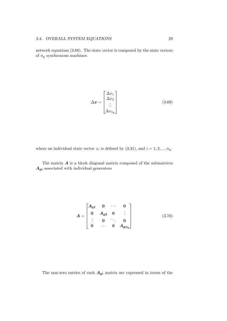
network equations (3.68). The state vector is composed by the state vectorsof ng synchronous machines:
∆x =
∆x1
∆x2...
∆xng
(3.69)
where an individual state vector xi is defined by (3.31), and i = 1, 2, ..., ng.
The matrix A is a block diagonal matrix composed of the submatricesAgi associated with individual generators
A =
Ag1 0 · · · 0
0 Ag2 0...
... 0. . . 0
0 · · · 0 Agng
(3.70)
The non-zero entries of each Agi matrix are expressed in terms of the

30 CHAPTER 3. MODELLING OF POWER SYSTEM
machine parameters and initial values of the currents id and iq as
A(1,2)g = ω0
A(2,3)g = − 1
M
X ′′ads
Xfdiq
A(2,5)g =
1
M
X ′′aqs
X1qid
A(2,10)g =
1
M
A(3,4)g = ω0
Rfd
Xfd
X ′′ads
X1d
A(3,9)g = KAω0
Rfd
Xadu
A(4,4)g = −ω0
R1d
X1d(1−
X ′′ads
X1d)
A(5,6)g = ω0
R1q
X1q
X ′′aqs
X2q
A(6,6)g = ω0
R2q
X2q(1−
X ′′aqs
X2q)
A(8,2)g = KSTABA
(2,2)g
A(8,4)g = KSTABA
(2,4)g
A(8,6)g = KSTABA
(2,6)g
A(8,10)g = KSTABA
(2,10)g
A(9,3)g =
T1
T2A(8,3)
g
A(9,5)g =
T1
T2A(8,5)
g
A(9,8)g = −T1
T2TW +
1
T2
A(9,10)g =
T1
T2A(8,10)
g
A(10,10)g = − 1
Tt
A(2,2)g = − 1
MKD
A(2,4)g = − 1
M
X ′′ads
X1diq
A(2,6)g =
1
M
X ′′aqs
X2qid
A[g(3,3) = −ω0
Rfd
Xfd(1−
X ′′ads
Xfd)
A(3,7)g = −KAω0
Rfd
Xadu
A(4,3)g = ω0
R1d
X1d
X ′′ads
Xfd
A(5,5)g = −ω0
R1q
X1q(1−
X ′′aqs
X1q)
A(6,5)g = −ω0
R2q
X2q
X ′′aqs
X1q
A(7,7)g = − 1
TR
A(8,3)g = KSTABA
(2,3)g
A(8,5)g = KSTABA
(2,5)g
A(8,8)g = − 1
TW
A(9,2)g =
T1
T2A(8,2)
g
A(9,4)g =
T1
T2A(8,4)
g
A(9,6)g =
T1
T2A(8,6)
g
A(9,9)g = − 1
T2
A(10,2)g = − 1
STt
(3.71)
C1 and C2 are block diagonal matrices with the block elements C1−g andC2−g respectively, where
C1−g =
[−V cos(δ − θ) 0 0 0 −X′′
aqs
X1q−X′′
aqs
X2q0 0 0 0
V sin(δ − θ) 0X′′
adsXfd
X′′adsX1d
0 0 0 0 0 0
](3.72)

3.4. OVERALL SYSTEM EQUATIONS 31
C2−g =
[idV cos(δ − θ)− iqV sin(δ − θ) 0 0 0 0 0 0 0 0 0−idV sin(δ − θ)− iqV cos(δ − θ) 0 0 0 0 0 0 0 0 0
](3.73)
In (3.72) and (3.73), V and θ denote the terminal voltage magnitude andangle of the generator in question.
The generator current vector ∆Ig is given by 1
∆Ig =
∆id1
∆iq1
∆id2
∆iq2...
∆idng
∆iqng
(3.74)
The matrices F1, G1, and G3, that all also have a block diagonal structure,are comprised by individual generator matrices of the form
F1−g =
0 0− 1M (−X ′′adsiq −Ψaq) − 1
M (Ψad +X ′′aqsid)
−ω0RfdXfd
X ′′ads 0
−ω0R1dX1d
X ′′ads 0
0 −ω0R1q
X1qX ′′aqs
0 −ω0R2q
X2qX ′′aqs
0 0
KSTABF(2,1)1−g1
T1T2F
(2,2)1−g1
T1T2F
(8,1)1−g1
T1T2F
(8,2)1−g1
0 0
(3.75)
G1−g =
[−Ra Xl +X ′′aqs
−Xl −X ′′ads Ra
]G3−g =
[Vg sin(δ − θ) V cos(δ − θ)Vg cos(δ − θ) −V sin(δ − θ)
](3.76)
The elements of the generator voltage vector Vg are the voltage angles
1The notation for the generator current vector and the voltage vectors was adaptedfrom [15], whereas in other sources (e.g.[2]) the preference is given to the real and imaginarycomponents of current and voltage.

32 CHAPTER 3. MODELLING OF POWER SYSTEM
and magnitudes of the generator buses:
∆Vg =
∆θ1
∆V1
∆θ2
∆V2...
∆θng
∆Vng
(3.77)
Each block of the block diagonal matrix F2 has only one non-zero element:
F(7,2)2−g =
1
TR(3.78)
The coefficients of the voltage variables in the stator voltage equations aredefined by another block diagonal matrix G2, comprised of
G2−g =
[V cos(δ − θ) − sin(δ − θ)−V sin(δ − θ) − cos(δ − θ)
](3.79)
The vector of the voltage magnitudes and angles of the load buses is definedas
∆VL =
∆θng+1
∆Vng+1
∆θng+2
∆Vng+2...
∆θng+nL
∆Vng+nL
(3.80)
The matrices G4-G7 represent the coefficients of the voltage variablesin the network equations. The odd- and even-numbered rows of the matri-ces correspond to the active power equations (3.62) and the reactive powerequations (3.63) respectively, whereas the odd- and even-numbered columnsrefer to the voltage angle and the voltage magnitude coefficients.
The matrix G4 contains the elements that show the sensitivity of thegenerator nodal equations to the voltage components of all the generators.
The off-diagonal elements of G4, with k = 1, 2, ..., ng and m = 1, 2, ..., ng
are given as
G(2k−1,2m−1)4 = −VkVmYkm sin(θk − θm − αkm)
G(2k−1,2m)4 = −VkYkm cos(θk − θm − αkm)
G(2k,2m−1)4 = VkVmYkm cos(θk − θm − αkm)
G(2k−1,2m)4 = −VkYkm sin(θk − θm − αkm)
(3.81)

3.4. OVERALL SYSTEM EQUATIONS 33
The diagonal entries of the matrix are defined by the following expressions:
G(2k−1,2k−1)4 = −idkVk cos(δk − θk) + iqkVk sin(δk − θk)−
−Vk∑m∈K
VmYkm sin(θk − θm − αkm)
G(2k−1,2k)4 = idk sin(δk − θk) + iqk cos(δk − θk)−
−∑m∈K
VmYkm cos(θk − θm − αkm)
G(2k,2k−1)4 = idkVk sin(δk − θk) + iqkVk cos(δk − θk)−
−Vk∑m∈K
VmYkm cos(θk − θm − αkm)
G(2k,2k)4 = idk cos(δk − θk)− iqk sin(δk − θk)−
−∑m∈K
VmYkm sin(θk − θm − αkm)
(3.82)
The entries of G5 and G6 and the off-diagonal elements of G7 are similarto the off-diagonal elements of G4 (3.81) with the only difference in theindexation. ForG5, that represents the sensitivities of the generator networkequations to the load voltages, k = 1, 2, ..., ng whereas m = ng + 1, ng +2, ...ng + nL. The indices in G6 and G7, incorporating the sensitivities ofthe load network equations, are k = ng + 1, ng + 2, ...ng + nL (G6 and G7),m = 1, 2, ..., ng (G6) and m = ng + 1, ng + 2, ...ng + nL (G7).
The diagonal elements of G7, i.e. sensitivities of the network equationsof the load buses to the voltages at the load buses are given by
G(2k−1,2k−1)7 = Vk
∑m∈K
VmYkm sin(θk − θm − αkm)
G(2k−1,2k)7 = dPLk
dVk−∑m∈K
VmYkm cos(θk − θm − αkm)
G(2k,2k−1)7 = −Vk
∑m∈K
VmYkm cos θk − θm − αkm)
G(2k,2k)7 = dQLk
dVk−∑m∈K
VmYkm sin(θk − θm − αkm)
(3.83)
where dPLkdVk
and dQLkdVk
are the sensitivities of the static load characteristics tothe voltage at the corresponding load bus. With the constant current andthe constant impedance characteristics for the active and reactive power

34 CHAPTER 3. MODELLING OF POWER SYSTEM
components respectively, as in (3.64),they become
dPLkdVk
= P 0k /V
0k (3.84)
dQLkdVk
= 2Q0kVk/(V
0k )2 (3.85)
The input vector ∆u may contain different quantities, e.g. the turbinesetpoint changes ∆Pm
set. Another example would be ∆u as a vector ofthe load changes ∆PL
set which explains the appearance of the D matrix in(3.68). Since the load power demand is not explicitly given in (3.65), the lastterm of (3.65) should disappear in this case. However, ∆u can be definedas
∆u =
[∆Pm
set
∆PLset
](3.86)
which yields non-zero elements in the both matrices B and D.
To enable the small-signal analysis, the system state matrix AS shouldbe derived. The successive elimination of ∆Vl and ∆Ig while assuming∆u = 0 will give
∆x = A′∆x+ F ′∆Vg (3.87)
0 = C′∆x+G′∆Vg (3.88)
where
A′ = A− F1G1−1C1 (3.89)
F ′ = F2 − F1G1−1G2 (3.90)
C′ = C2 −G3G1−1C1 (3.91)
G′ = G4 −G3G1−1G2 −G5G7
−1G6 (3.92)
Equation (3.88) can be rewritten as
∆Vg = −G′−1C′∆x (3.93)
Substitution of ∆Vg in (3.87) gives
∆x = (A′ − F ′G′−1C′)∆x (3.94)
Thus
AS = A′ − F ′G′−1C′ (3.95)
The analysis of the eigenvalues of the system state matrix AS couldshow, whether the system is stable or unstable at the given operating point.

3.4. OVERALL SYSTEM EQUATIONS 35
Load Damping Case
If the load damping modelling is to be adopted, the system equations and,therefore, the previously defined matrices should be adjusted. The load busvoltage angles become state variables, and they should be added to the statevector:
∆x = [∆xTold ∆θng+1 ∆θng+2 · · · ∆θng+nL ]T (3.96)
The vector of the load bus voltage components, on the contrary, gets reduced:
∆VL =
∆Vng+1
∆Vng+2...
∆Vng+nL
(3.97)
Since the active power injections at the load buses are already defined bythe new differential equations, the corresponding algebraic equations shouldbe excluded from the load bus network equations.
Thus, (3.65-3.68) become
∆x = A∆x+ F1∆Ig + F2∆Vg + F3∆VL +B∆u (3.98)
0 = C1∆x+G1∆Ig +G2∆Vg (3.99)
0 = C2∆x+G3∆Ig +G4∆Vg +G5∆VL (3.100)
0 = C3Q∆x+G6Q∆Vg +G7Q∆VL (3.101)
The matrices A and F2 should be extended to account for the new differ-ential equations. The block AL contains nL × nL elements of the followingform
A(k,m)L =
ω0
KDkVkVmYkmsin(θk − θm − αkm) (3.102)
where k = ng + 1, ng + 2, ..., ng + nL, m = ng + 1, ng + 2, ..., ng + nL andm 6= kand
A(k,k)L = − ω0
KDkVk∑m∈K
VmYkm sin(θk − θm − αkm) (3.103)
where m = 1, 2, ..., ng + nL
AL should be added at the diagonal of A (3.70),The matrices F2 and F3 should be augmented with nL additional rows
each. The elements of these rows are as follows:
F(k,2m−1)2−L =
ω0
KDkVkVmYkm sin(θk − θm − αkm) (3.104)
F(k,2m)2−L =
ω0
KDkVkYkm cos(θk − θm − αkm) (3.105)
where k = ng + 1, ng + 2, ..., ng + nL,m = 1, 2, ..., ng The first 10ng × nL
entries of the new matrix F3 are zeros, since the derivatives of the generator

36 CHAPTER 3. MODELLING OF POWER SYSTEM
state variables are not explicitely influenced by the voltage magnitude atthe load buses. The last nL rows of F3 have the elements defined as
F(k,m)3−L =
ω0
KDkVkYkm cos(θk − θm − αkm) (3.106)
with k = ng + 1, ng + 2, ..., ng + nL, m = ng + 1, ng + 2, ..., ng + nL
F(k,k)3−L =
ω0
KDkVk∑m∈K
Ykm cos(θk − θm − αkm) (3.107)
with m = 1, 2, ..., ng + nL
Besides, nL rows with zero entries should be added to the matrix F1.Now the system state matrix can be computed by using a similar ap-
proach as in the no damping case:
C4 = C2 −G5G7Q−1G3Q (3.108)
G8 = G4 −G5G7Q−1G6Q (3.109)
A′ = A− F1G3−1C4 − F3G7QC3Q (3.110)
F ′ = F2 − F1G3−1G8 − F3G7QG6Q (3.111)
C′ = C1 −G1G3−1C4 (3.112)
G′ = G2 −G1G3−1G8 (3.113)
∆x = (A′ − F ′G′−1C′)∆x (3.114)
HenceAS = A′ − F ′G′−1C′ (3.115)
3.4.2 Transient Stability
For the transient stability analysis, the system equations expressed in theform
x = f(x, Ig,V ) (3.116)
0 = g(x, Ig,V ) (3.117)
should be solved to model the response of the system to a given distur-bance. In (3.116,3.117), f and g are nonlinear functions. The solution of anonlinear sysem of differential and algebraic equations can be obtained byimplementing the methods of numerical integration. In this work, a par-titioned approach with explicit integration is used. The term partitionedsolution refers to the separate solution of differential and algebraic equa-tions. In explicit integration methods, such as R-K methods, the value of xat any t can be estimated from its value at the previous time step.
This approach includes the following steps [2]:

3.4. OVERALL SYSTEM EQUATIONS 37
1. Calculate the initial state of the system (before a disturbance).
2. Change the admittance matrix to model the given disturbance, e.g.add a shunt element with a large conductance at the faulty bus tomodel a three-phase short circuit.
3. The state variables x cannot change instantaneously after the dis-turbance. The algebraic equations (3.117) should be solved with theknown x to find the voltages and currents at the instant after the dis-turbance. The Newton-Raphson algorithm, used in this thesis for thesolution of the algebraic equations, is broadly used in power systemanalysis and extensively covered in the literature (e.g.[17]).
4. The time derivatives f(x, Ig,V ) can be estimated now by using theknown values of x, Ig, and V .
5. To find the values of the state variables x at the next time instant, R-K numerical integration method can be applied (see Appendix A) byusing the time derivative values from the previous step in the formulae(A.2).
6. The steps 3-5 should be repeated to obtain the time response of thesystem to the given disturbance. If the fault is assumed to be clearedat some time point, the admittance matrix will be changed again, andthe network variables will change stepwise, but not the state variables.
According to [2], the advantages of this approach are its flexibility, sim-plicity, reliability, and robustness. However, it might become numericallyunstable if the time step is bigger than the time constant of the smallesteigenvalue.

38 CHAPTER 3. MODELLING OF POWER SYSTEM

Chapter 4
Impact of Rotational Inertiaand Damping on PowerSystem Stability
In this chapter, sensitivities of the system state matrix to inertia and damp-ing are derived. They are further implemented in computation of dampingratio sensitivities and sensitivities of transient frequency overshoot based on[1]. In the following sections, an algorithm for inertia and damping opti-mization and its implementation in MATLAB are presented.
4.1 Sensitivity of Damping Ratio
The damping ratio of an oscillatory mode shows how fast the associatedoscillations will decay after a small disturbance. To ensure the secure opera-tion of a power system, the oscillatory modes should be sufficiently dampedunder any possible normal operating conditions of the system.
With the time dependent inertia level, it becomes very important tounderstand how the changes in inertia affect the oscillatory modes. Fur-thermore, when damping level in the system can be adjusted, it would bevaluable to know how the system reacts to the changes in damping.
The sensitivity of the damping ratio of the i-th dynamic mode to aparameter η (M or KD) could be derived from the definition of dampingratio (2.14) as
∂ζ(i)
∂η=
∂
∂η(
−σ(i)√σ(i)2 + ω(i)2
) = ω(σ(i) ∂ω(i)
∂η − ω(i) ∂σ(i)
∂η )
(σ(i)2 + ω(i)2)3/2(4.1)
where
∂σ(i)
∂η= Re(
∂λ(i)
∂η) (4.2)
39

40 CHAPTER 4. IMPACT OF INERTIA AND DAMPING
∂ω(i)
∂η= Im(
∂λ(i)
∂η) (4.3)
The sensitivity of the eigenvalue λi to η is determined by the values of theright and left eigenvectors, φ(i) and ψ(i), calculated using the normalization(2.10), and by the sensitivity of the state matrix to this parameter as [1]
∂λ(i)
∂η= ψ(i)T ∂AS
∂ηφ(i) (4.4)
Thus, to find the sensitivities of the damping ratios to the inertia anddamping coefficients, the expressions for the sensitivity of the system statematrix should be derived.
4.1.1 State Matrix Sensitivity to Rotational Inertia
No Load Damping
The sensitivity of the system state matrix to the inertia of one of thesyncronous machines, M , is determined by
∂AS
∂M=∂A′
∂M− ∂F ′
∂MF ′G′−1C′ =
∂A′
∂M− ∂F ′
∂MF ′G′−1C′ (4.5)
with
∂A′
∂M=
∂
∂M(A− F1G1
−1C1) =∂A
∂M− ∂F1
∂MG1−1C1 (4.6)
∂F ′
∂M=
∂
∂M(F2 − F1G1
−1G2) = −∂F1
∂MG1−1G2 (4.7)
∂C′
∂M= 0 (4.8)
∂G′
∂M= 0 (4.9)
In (4.6), ∂A∂M and ∂F1
∂M are block diagonal matrices. However, their onlyblocks that contain non-zero elements are the ones that correspond to thegenerator in question, since the inertia level of a generator does not explicitlyinfluence the state variables of the other generators. The non-zero elements

4.1. SENSITIVITY OF DAMPING RATIO 41
of the submatrix∂Ag
∂M can be derived from (3.71) that yields
∂A(2,2)g
∂M=
1
M2KD
∂A(2,3)g
∂M=
1
M2
X ′′ads
Xfdiq
∂A(2,4)g
∂M=
1
M2
X ′′ads
X1diq
∂A(2,5)g
∂M= − 1
M2
X ′′aqs
X1qid
∂A(2,6)g
∂M= − 1
M2
X ′′aqs
X2qid
∂A(2,10)g
∂M= − 1
M2
∂A(8,2)g
∂M= KSTAB
∂A(2,2)g
∂M
∂A(8,3)g
∂M= KSTAB
∂A(2,3)g
∂M
∂A(8,4)g
∂M= KSTAB
∂A(2,4)g
∂M
∂A(8,5)g
∂M= KSTAB
∂A(2,5)g
∂M
∂A(8,6)g
∂M= KSTAB
∂A(2,6)g
∂M
∂A(8,10)g
∂M= KSTAB
∂A(2,10)g
∂M
∂A(9,2)g
∂M=T1
T2
∂A(8,2)g
∂M
∂A(9,3)g
∂M=T1
T2
∂A(8,3)g
∂M
∂A(9,4)g
∂M=T1
T2
∂A(8,4)g
∂M
∂A(9,5)g
∂M=T1
T2
∂A(8,5)g
∂M
∂A(9,6)g
∂M=T1
T2
∂A(8,6)g
∂M
∂A(9,10)g
∂M=T1
T2
∂A8,10)g
∂M(4.10)
The non-zero elements of the block∂F1−g
∂M are computed for each synchronousmachine in the system as
∂F(2,1)1−g
∂M=
1
M2(−X ′′adsiq −Ψaq)
∂F(8,1)1−g
∂M= KSTAB
∂F(2,1)1−g
∂M
∂F(9,1)1−g
∂M=T1
T2
∂F(8,1)1−g
∂M
∂F(2,2)1−g
∂M=
1
M2(Ψad +X ′′aqsid)
∂F(8,2)1−g
∂M= KSTAB
∂F(2,2)1−g
∂M
∂F(9,2)1−g
∂M=T1
T2
∂F(8,2)1−g
∂M
(4.11)
Load Damping CaseIn case damping is provided at the load buses, and it is to be modelled
as in Section 3.3, Equations (4.6) and (4.7) should be modified according tothe adjusted structure of the set of the system equations (3.98-3.101).
∂A′
∂M=
∂A
∂M− ∂F1
∂MG3−1C4 (4.12)
∂F ′
∂M= −∂F1
∂MG3−1G8 (4.13)
The non-zero elements of ∂A∂M and ∂F1
∂M can be determined by means of(4.10) and (4.11).
The size of ∂A∂M and ∂F1
∂M should be similar to that of A and F1 respec-tively. Therefore, if the load damping differential equations are introduced,∂A∂M should be augmented by nL zero rows and nL zero columns, while ∂F1
∂Mgets nL zero rows.

42 CHAPTER 4. IMPACT OF INERTIA AND DAMPING
4.1.2 State Matrix Sensitivity to Damping
No Load DampingIt could be assumed that the damping at a generator bus could be
changed, e.g. by means of BESS.
∂AS
∂KD=
∂A′
∂KD=
∂A
∂KD(4.14)
The only non-zero elements of a block∂Ag
∂KD, representing the sensitivity of
the state variables of the generator in question to the associated dampingcoefficient, are
∂A(2,2)g
∂KD= − 1
M
∂A(8,2)g
∂KD= −KSTAB
1
M
∂A(9,2)g
∂KD= −T1
T2KSTAB
1
M
(4.15)
Load Damping Case
∂AS
∂KD=
∂A′
∂KD− ∂F ′
∂KDG′−1C′ (4.16)
where
∂A′
∂KD=
∂A
∂KD− ∂F3
∂KDG7Q
−1C3Q (4.17)
∂F ′
∂KD=
∂F2
∂KD− ∂F3
∂KDG7Q
−1G6Q (4.18)
The sensitivities of the matrix A to the load damping at the bus in questionare given by the matrix ∂A
∂KDof the same size asA. Generator state variables
are not explicitly affected by the change of load damping, thus the first 10·ng
rows and the first 10·ng columns of ∂A∂KD
will always have only zero elements.Non-zero entries will appear in the row (10ng + k) for the k-th load bus:
∂A
∂KDk
(9ng+k,9ng+m)
= − ω0
KDk2VkVmYkmsin(θk − θm − αkm) (4.19)
where k = ng + 1, ng + 2, ..., ng + nL, m = ng + 1, ng + 2, ..., ng + nL andm 6= kand
∂A
∂KDk
(9ng+k,9ng+k)
=ω0
K2Dk
Vk∑m∈K
VmYkm sin(θk − θm − αkm) (4.20)

4.2. SENSITIVITY OF TRANSIENT OVERSHOOT 43
where m = 1, 2, ..., ng + nL
The derivative of F2 with respect to the damping at a given load bushas the following non-zero elements:
∂F2
∂KDk
(9ng+k,2m−1)
= − ω0
K2Dk
VkVmYkm sin(θk − θm − αkm) (4.21)
∂F2
∂KDk
(9ng+k,2m)
= − ω0
K2Dk
VkYkm cos(θk − θm − αkm) (4.22)
where k = ng + 1, ng + 2, ..., ng + nL, m = 1, 2, ..., ng
Finally, non-zero entries of ∂F3∂KDk
are defined by
∂F3
∂KDk
(9ng+k,m)
= − ω0
K2Dk
VkYkm cos(θk − θm − αkm) (4.23)
where k = ng + 1, ng + 2, ..., ng + nL, m = ng + 1, ng + 2, ..., ng + nL
∂F3
∂KDk
(9ng+k,k)
= − ω0
K2Dk
Vk∑m∈K
Ykm cos(θk − θm − αkm) (4.24)
where m = 1, 2, ..., ng + nL
4.2 Sensitivity of Transient Overshoot
The frequency response of a system to a disturbance depends on the levelof inertia and damping in this system. Inertial response of synchoronousmachines is an inherent reaction to an imbalance of mechanical and electricaltorques at their rotors. After a major disturbance, such as the loss of bulkgeneration units, the rotational inertia of the remaining machines reducesthe rate of frequency drop. This provides more time for the control actions,aimed at settling the frequency at an acceptable level and ensuring thestability of the system. In case of high penetration of RES, the grid inertiasignificantly decreases. This affects the frequency response, causing largerfrequency deviations, and requires faster operation of the frequency control.
In this section, the sensitivity of a transient overshoot after a disturbanceto the inertia of the generators will be derived based on [1] and on the systemequations formulated in Chapter 3.
The sensitivities of the right and the left eigenvectors to a parameter ηare given by
∂φ(k)
∂η=∑j∈N
cηkjφ(j) ,
∂ψ(k)
∂η=∑j∈N
dηkjψ(j) (4.25)

44 CHAPTER 4. IMPACT OF INERTIA AND DAMPING
where N is the set of the system modes, and the off-diagonal elements cηkjand dηkj can be expressed as
cηkj =ψ(j)T ∂AS
∂η φ(k)
(λ(k) − λ(j))ψ(j)Tφ(j)k 6= j (4.26)
dηkj =ψ(k)T ∂AS
∂η φ(j)
(λ(k) − λ(j))ψ(j)Tφ(j)k 6= j (4.27)
The derivative of the product φ(i)ψ(i)T, which is given by
∂φ(i)ψ(i)T
∂η=∂φ(i)
∂ηψ(i)T + φ(i)∂ψ
(i)T
∂η(4.28)
can be rewritten noting that ckj = −dkj as [1]
∂φ(i)ψ(i)T
∂η=∑j\i
[φ(j)cηijψ(i)T − φ(i)cηjiψ
(j)T] (4.29)
The derivative (4.29) will be employed in the latter derivations.The frequency response can be estimated by means of an open-loop trans-
fer function between the input (disturbance ∆u = ∆Pk) and the output(angular velocity deviation ∆y = ∆ωr) variables. The open-loop transferfunction could be obtained from
∆x = AS∆x+ bk∆u (4.30)
∆y = cl∆x (4.31)
where cl is a matrix mapping the frequency of node l on the output ykl andbk shows the contribution of a disturbance at the k-th node to the deviationof the state variables. Hence, the transfer function G(s) can be expressedas
G(s) =∆Y (s)
∆U(s)= cl(sI −A)(−1)bk
= clφ(sI −Λ)(−1)ψTbk
=∑i∈N
Rklis− λ(i)
(4.32)
where Rkli is a residue of G(s) at pole s = λ(i)
Rkli = clφ(i)ψ(i)Tbk (4.33)
The matrix bk is not as easily derived as in [1] because in this thesis, a morecomplex model of a power system is employed. The derivation of bk will becovered later in this section.

4.2. SENSITIVITY OF TRANSIENT OVERSHOOT 45
With the short-hand Kkli =
Rkli
λ(i), the step response Y (s) is given by
Y kl (s) =
1
sG(s) = −
∑i∈N
Kkli
λ(i)
s(s− λ(i))(4.34)
which in time domain yields
ykl (t) = L−1[Y kl (s)] = −
∑i∈N
Kkli(1− eλ
(i)t) (4.35)
After dividing the eigenvalues into real and complex conjugate, representedby the sets Λ0 and Lambda+, respectively, the time-domain response can berewritten as
ykl (t) = −∑i∈Λ0
Kkli(1− eλ
(i)t)− 2∑i∈Λ+
(KkReli − eσ(i)t ||Kk
li|| sin(ω(i)t− βkli))
(4.36)with
βkli = arctan(KkReli ,KkIm
li ) (4.37)
The dominating mode i could be defined by finding the largest Kklj
i = argmaxjKklj (4.38)
The first peak time and magnitude of the dominating mode i could be ap-proximated by
tkpl =1
ω(i)(0.5π − βkli) (4.39)
Mkpl = ykl (tkpl) (4.40)
The next step would be to estimate the sensitivity of M lpk to inertia and
damping. The derivative of the transfer function residue Rkli to inertia ordamping of the j-th generator is given by
∂Rkli∂ηj
=∂
∂ηj(clφ
(i)ψ(i)Tbk) = cl∂φ(i)ψ(i)T
∂ηjbk + clφ
(i)ψ(i)T∂bk
∂ηj(4.41)
The gain of the step-response Kkli is affected by inertia or damping changes
as follows:
∂Kkli
∂ηj=
∂
∂ηj
Rkliλ(i)
=
∂Rkli
∂ηjλ(i) −Rkli
∂λ(i)
∂ηj
(λ(i))2(4.42)

46 CHAPTER 4. IMPACT OF INERTIA AND DAMPING
The change of the first peak time can be estimated by
∂ arctan(xy )
∂η=
∂x∂ηy −
∂y∂ηx
y2 + x2(4.43)
∂
∂η
1
ω(i)= − 1
(ω(i))2
∂ω(i)
∂η(4.44)
∂tkpl∂ηj
= − 1
(ω(i))2
∂ω(i)
∂ηj(0.5π − β)− 1
ω(i)
∂ arctan(KRe
i
KImi
)
∂ηj(4.45)
Finally, the derivative of the overshoot is given by
∂Mkpl
∂ηj=∂ykl (tkpl)
∂ηj= −
∑i∈N
[∂Kk
li
∂ηj(1− eλ
(i)tkpl)
−Kkli
∂λ(i)
∂ηjtkple
λ(i)tkpl −Kkliλ
(i)∂tkpl∂ηj
eλ(i)tkpl ]
(4.46)
As a next step, the matrix bk is derived.
No Load Damping
To enable the calculation of the open-loop transfer function as in (4.32),the system frequency response should be described by
∆x = A∆x+ bk∆Pk (4.47)
∆ωr = cl∆x (4.48)
where ∆Pk is the vector of disturbances. If we assume the disturbance tohappen at one of the load buses, the system equations should be adjustedas follows:
∆x = A∆x+ F1∆Ig + F2∆Vg (4.49)
0 = C1∆x+G1∆Ig +G2∆Vg (4.50)
0 = C2∆x+G3∆Ig +G4∆Vg +G5∆VL (4.51)
0 = G6∆Vg +G7∆VL + dk∆Pk (4.52)
Rearrangement of (4.50) and (4.52) yields
∆VL = −G7−1(G6∆Vg + dk∆Pk) (4.53)
∆Ig = −G1−1(C1∆x+G2∆Vg) (4.54)
Substitution of VL and Ig in (4.49) and (4.51) gives
∆x = A′∆x+ F ′∆Vg (4.55)
0 = C′∆x+G′∆Vg −G5G−17 dk∆Pk (4.56)

4.2. SENSITIVITY OF TRANSIENT OVERSHOOT 47
where A′, C′, F ′ and G′ are the shortcuts adopted in (3.89-3.92). Now(4.49) can be rewritten as
∆x = AS∆x+ F ′G′−1G5G−17 dk∆Pk (4.57)
Thus, the desired matrix bk could be computed as
bk = F ′G′−1G5G−17 dk (4.58)
where dk is a 2nL · 2nL matrix with only one non-zero element
dk(2k−1,2k−1) = 1 (4.59)
If the distrubances at generator buses are to be considered, the term dk∆Pk
appears in (4.51), and (4.60) becomes
∆x = A′∆x+ F ′∆Vg (4.60)
0 = C′∆x+G′∆Vg − dk∆Pk (4.61)
that yields
∆x = AS∆x+ F ′G′−1dk∆Pk (4.62)
and
bk = F ′G′−1dk (4.63)
Now ∂bk
∂Mjand ∂bk
∂KDshould be calculated to be used in (4.41)
∂bk
∂Mj=
∂F ′
∂MjG′−1G5G
−17 dk (4.64)
∂bk
∂Mj=
∂F ′
∂MjG′−1dk (4.65)
∂bk
∂KD= 0 (4.66)
where equation (4.64) corresponds to the disturbances at the load buses,and equation (4.65) corresponds to the disturbances at the generator buses.The derivative ∂F ′
∂Mjis given by (4.7).
Load Damping Case
Since the active power injection at the load buses is in this case repre-sented by the differential equations (3.54), disturbances at the load busescould be modelled by directly adding the term bk∆Pk to Equation (3.98).The equation becomes
∆x = AS∆x+ bk∆Pk (4.67)
48 CHAPTER 4. IMPACT OF INERTIA AND DAMPING
where bk has size (10ng + nL) · nL and the non-zero element of bk is givenby
bk(10ng+k,k) =ω0
KDk(4.68)
A disturbance at a generator bus could be modelled in the same way as inthe no load damping case, with (4.62), while the matrices A′, F ′, C′ andG′ should be adopted from (3.110-3.113).
The derivatives of bk with respect to M and KD for the case of a distur-bance at a load bus are given by
∂bk
∂Mj= 0 (4.69)
∂bk
∂KD
(10ng+k,k)
=ω0
K2Dk
(4.70)
If a disturbance occurs at a generator bus, taking the derivatives of bk yields
∂bk
∂Mj=
∂F ′
∂MjG′−1dk (4.71)
∂bk
∂KD=
∂F ′
∂KDG′−1dk (4.72)
with ∂F ′
∂Mjand ∂F ′
∂KDas defined by (4.18).
By comparing Equations (4.64) and (4.71), it could be concluded thatthe load damping model, suggested in Section 3.3.2, does not adequatelyreflect the sensitivity of the generator frequency response to the rotationalinertia for the load bus case.
The expressions for bk and its derivatives can be used to calculate thetransient overshoot Mk
pl and its sensitivities.
Knowing how the changes of inertia and damping affect the eigenvaluesof the system state matrix and the magnitude of the transient overshoot,it is now possible to formulate an optimization program focused on theimprovement of the system stability.
4.3 Optimization Algorithm
The optimization algorithm described in this section was proposed in [1].Its objective is the maximization of the worst-case (minimal) damping ratioof any mode in the system. The larger the damping ratios are, the fasterthe oscillatory modes decay which is advantageous for the system stability.At the same time, to avoid large deviations of the frequency due to reducedinertia, the frequency overshoot after a disturbance should be constrained.Damping and inertia are assumed to be adjustable within some bounds and

4.3. OPTIMIZATION ALGORITHM 49
associated with a cost. The sets K and M include the nodes with dampingand inertia, respectively. The total amount of inertia and damping that canbe added is assumed to be limited.
The sensitivities of the damping ratios and the overshoot are non-linear,therefore, each step of the optimization will be associated with a solutionof a linearized problem. Superscript ν denotes the number of the iterationwith 0 being the first iteration. After each iteration, the system state matrix,along with the sensitivities of damping ratios and transient overshoot shouldbe computed all over again.
The change of the damping from the current iteration to the next is givenby
∆Kν+1Dj = Kν+1
Dj −KνDj (4.73)
A similar expression is applied to the value of inertia. To enable the calcula-tion of the absolute change in inertia and damping, Kν+1
Dj and Mν+1j should
be split in positive parts, K+Dj and M+
j , and negative parts,K−Dj and M−j ,as
K+Dj =
Kν+1
Dj −K0Dj if Kν+1
Dj −K0Dj > 0
0 if Kν+1Dj −K0
Dj ≤ 0(4.74)
K−Dj =
0 if Kν+1
Dj −K0Dj > 0
|Kν+1Dj −K0
Dj | if Kν+1Dj −K0
Dj ≤ 0(4.75)
M+j =
M −ν+1
j −M0j if Mν+1
j −M0j > 0
0 if Mν+1j −M0
j ≤ 0(4.76)
M−j =
0 if Mν+1
j −M0j > 0
|Mν+1j −M0
j | if Mν+1j −M0
j ≤ 0(4.77)
The absolute change could be now estimated as
|KDj | = K+Dj +K−Dj (4.78)
|Mj | = M+j +M−j (4.79)
The objective function penalizes the minimal damping ratio with costcζ ≥ 0. The purpose of the slack variable εkpl is to ensure the feasibility ofthe problem, and it is penalized by the cost cε. Procurement of additionalinertia and damping implicates economic costs cMi and cKi. However, theaccurate calculation of cMj and cKj would be a complex task without awell-developed inertia and damping procurement market.
minKDj ,Mj
[−cζζmin +∑k
∑l
(cεεkpl) +
∑i∈K
cKj |KDj |+∑i∈M
cMj |Mj |] ∀i ∈ Λ+
(4.80)

50 CHAPTER 4. IMPACT OF INERTIA AND DAMPING
s.t.
ζν+1i = ζνi +
∑j∈K
∂ζνi∂KDj
∆Kν+1Dj +
∑j∈M
∂ζνi∂Mj
∆Mν+1j (4.81)
ζmin ≤ ζν+1i (4.82)∑
j∈K|KDj | ≤ Ktot
D (4.83)
∑j∈M|Mj | ≤ M tot (4.84)
KminDj ≤ Kν+1
Dj ≤ KmaxDj (4.85)
Mminj ≤ Mν+1
j ≤Mmaxj (4.86)
∆KminDj ≤ ∆Kν+1
Dj ≤ ∆KmaxDj (4.87)
∆Mminj ≤ ∆Mν+1
j ≤ ∆Mmaxj (4.88)
0 ≤ K+Dj , 0 ≤ K−Dj (4.89)
K+Dj −K
−Dj = Kν+1
Dj −K0Dj (4.90)
0 ≤ M+j , 0 ≤M−j (4.91)
M+j −M
−j = Mν+1
j −M0j (4.92)
fp−Mkpl∆Pk ≥
∑j∈M
∂Mkpl
∂Mj∆Pk∆M
ν+1j +
∑j∈K
∂Mkpl
∂KDj∆Pk∆K
ν+1Dj − ε
kpl (4.93)
With (4.81), the value of the damping ratios are computed at the step ν+ 1using the previous value ζνi and the changes related to the adjustment of Mj
and KDj . The constraint (4.82) serves to set ζmin to the lowest dampingratio value. The inequality constraints (4.83) and (4.84) limit the totalchange of inertia and damping to the values available for procurement. Theindividual values of Mj and KDj at each bus are limited by (4.85) and(4.86). Sensitivities of ζ and Mk
pl computed at each iteration are valid onlyfor a small range of values around the initial Mν
j and KνDj . Therefore, the
steps ∆Kν+1Dj and ∆Mν+1
j should be limited by (4.87) and (4.88). Equalities(4.89-4.92) split KDj and Mj as in (4.78 and 4.79).
The magnitude of the transient overshoot after a disturbance ∆Pk isgiven by Mk
pl∆Pk. The change of inertia and damping by ∆Kν+1Dj and
∆Mν+1j results in additional terms of the overshoot as shown in (4.93).
The total magnitude of the overshoot should not exceed the limit fp.
At each iteration ν, the program finds the optimal levels of damping andinertia. These values are used to calculate the system state matrix and itseigenvalues, the new values of sensitivities, and the approximate magnitude

4.4. IMPLEMENTATION IN MATLAB 51
of transient overshoot. All these quantities are implemented in optimizationat iteration ν + 1. This optimization program can be used to facilitate theprovision of synthetic inertia and fast frequency response. It could also serveas a reference tool for planning of power systems.
4.4 Implementation in MATLAB
To analyze the impact of inertia changes on the stability of test power sys-tems, the proposed optimization algorithm was implemented in the engi-neering environment MATLAB, along with a supplementary transient sim-ulations tool .
Optimization Program
DATA.matBUSESLINESGENS
START
Reindexation Power Flow Computation Kron Reduction
Calculation of the initial state of the generators
Computation of the system state matrix and eigenvalues
Calculation of the eigenvalue and eigenvector sensitivities
Estimation of the transient overshoot and sensitivitiesOptimization of the inertia and damping levelsmin (dm;dk) <0,1
END
0
1 NO
YES
Figure 4.1: Structure of the developed optimization program
The flow chart of the developed MATLAB program for inertia and damp-ing optimization is presented in Figure 4.1. The input data for the optimiza-tion program should be saved in the file DATA.mat and should include thefollowing arrays:
1. BUSES with information on the nodes of the investigated power sys-tem, such as active and reactive power injections, voltage magnitudesof PV-buses, susceptance of the shunt devices, etc.
2. LINES where topology of the grid and parameters of the transmissionlines are stored.

52 CHAPTER 4. IMPACT OF INERTIA AND DAMPING
3. GENS where parameters of the on-line generators are listed.
The required structure of the arrays is described in Appendix D.
The MATLAB file run optimization.m is the master file of the optimiza-tion program. At the start of the master file, the user could choose the modelorder for the synchronous machines: 6,7,9 or 10. Each option represents thenumber of the differential equations describing a machine. The option 6corresponds to an unregulated machine, by entering 7 the model with AVRwould be chosen, with 9 PSS would be implemented, and 10 stands or thefull model employed in this work. The ability to choose the model could beuseful, if the effects of a particular regulation system on the system stabilityare to be analyzed. Besides that, the user could choose, whether he or shewould like to include the load damping modelling by typing ’on’ or ’off’ inresponse to a corresponding inquiry.
After the user has made his choice, the program starts to process thedata. First of all, the nodes and the lines of the system are re-indexed byreindexation.m to ensure the sequential numbering of the elements start-ing with ”1”. The next step is calculation of the initial steady state of thesystem by means of power flow computation accomplished by the packageMATPOWER 5.1. This tool is called upon by pf.m where the necessarypower system data is first processed to get the MATPOWER format. Re-sulting from MATPOWER computations are the voltage magnitudes andangles, along with active and reactive power injections at the nodes of thesystem.
Next, the nodes are sorted into three categories: generator nodes, loadbuses and other buses (with no power injections). To exclude the otherbuses from the analysis, Kron reduction is implemented via kron.m. TheMATPOWER output data is used as an input to evaluate the generatorvariables id, iq, and δ which is done by gencurrents.m. These variables rep-resent the interface between synchronous machines and transmission net-work, and after getting their values, the algorithm proceeds with computa-tion of coefficient matrices for the linearized network equations (G4 −G7,network equations.m).
In the following stage, the function sensitivities.m computes the systemstate matrix AS, its eigenvalues and eigenvectors, and sensitivities of damp-ing ratios to rotational inertia of generators and to damping. To deriveAS, the program has to build the matrices Ag,FX−g,CX−g and GX−g foreach generator bus, along with the derivatives of Ag and FX−g used in thefurther analysis. This step is carried out by gen equations.m. Then, thetransient overshoot magnitudes and their sensitivities to inertia and damp-ing are estimated by transient overshoot.m.
After the eigenvalues, overshoot magnitudes, and their sensitivities havebeen computed, the parameters of the optimization should be defined. Amongthese parameters are the costs introduced in the objective function, the total

4.4. IMPLEMENTATION IN MATLAB 53
avaliable inertia and damping, the parameters of the equality constraints,and the number of iterations.
The optimization is carried out by means of the free of charge opti-mization package YALMIP. YALMIP is a modelling language for advancedmodelling and solution of convex and nonconvex optimization problems [18].In optimization.m, with optimization parameters as an input, the specifiedobjective function is maximized subject to the given constraints by IBMILOG CPLEX solver. Results of the optimization problem solution, the up-dated values of inertia and damping at the nodes, are used to calculate thenew eigenvalues, overshoot, and sensitivities by means of sensitivities.m andtransient overshoot.m. Next, another optimization round is carried out, andfurther, by repetitive optimization solution and calculation of eigenvalues,transient overshoot, and their sensitivities, the local optimum of the objec-tive function is found. The number of the iterations should be manuallyadapted to ensure that the solution has converged. If from one iterationto another, the minimal damping ratio does not get any improvement, themaximal size of the steps ∆K and ∆M is decreased by 10% , as an attemptto push the solution into another direction. The reduction of the steps isaccumulated in factors dm and dk. When one of them becomes smallerthan 0.1, the user receives the message that declares the termination of thewhole optimization process and displays the achieved improvement of mini-mal damping ratio in percent.
Transient Simulations
The master file of the transient simulations is called run transient. It re-quires the same input data as the optimization program and starts the com-putations by calling reindexation.m, pf.m, and kron.m. The next step isestimation of the initial values of the generator variables in initial x gen.m.Following this, the bus and the branch where a disturbance occurs is speci-fied, and the admittance matrix of the system is altered to involve a shuntelement at the faulty bus. The new values of the network variables (voltagesand currents) are calculated at the next step by means of Newton-Raphsoniteration algorithm implemented in newtraph.m. The latter has two sub-functions, algebraic.m, where the right-side parts of the network equations(3.117) are evaluated, and jacobian.m computing the Jacobian associatedwith these equations.
After that, the time step and the number of the time intervals beforethe fault is cleared are specified. For each time interval, the values of thestate variables are computed by means of numerical integration, while thevalues of the network variables are estimated in newtraph.m. Numericalintegration is carried out by the second order R-K method (rungekutta2.m)

54 CHAPTER 4. IMPACT OF INERTIA AND DAMPING
or the fourth order R-K method in Gill’s modification (rungekuttagill.m).More than once at each time step, R-K methods require the calculation ofthe state variable derivatives with respect to time which is implemented inderiv gen.
After the fault is assumed to be cleared, the admittance matrix shouldbe adjusted according to the new network conditions. Following that, new-traph.m is executed again to find the updated value of the network variables,that abruptly altered after the admittance matrix changed. Finally, the newtime step and the number of the time intervals are specified, and R-K nu-merical integration along with Newton-Raphson algorithm are implementedto folllow the behaviour of the state and network variables after the faultwas cleared.

Chapter 5
Simulation Results
The proposed optimization algorithm and the developed transient simulationprogram were implemented for two test systems, IEEE two-area test system[2] and IEEE South East Australian test system [4]. Both systems are oftenused for testing small-signal stability analysis programs. In the presentchapter, the results of optimization are presented and illustrated by thetransient simulation results.
5.1 IEEE Two-Area Test System
5.1.1 System Description
The two-area system shown in Figure 5.1 is often used for benchmarking ofsmall-signal stability analysis tools. This simplified power system consistsof two areas interconnected by a weak tie link. Each area includes 2 gener-ators supplying an aggregated load bus. Eventhough this system is far lesscomplex than the real-life power systems, it is already a step ahead from thesingle machine infinite bus (SMIB) representation, as it allows to investigateinterarea oscillations.
In the present work, the system operating state and parameters listedin Example 12.6 of [2] were adopted. This allowed to assess the modellingaccuracy by comparing the obtained results with those in [2]. The investi-gated operating state is described by the following data:G1: P = 700 MW Q = 185 MVAr Et = 1.03∠20.2G2: P = 700 MW Q = 235 MVAr Et = 1.01∠10.5G3: P = 719 MW Q = 176 MVAr Et = 1.03∠− 6.8G4: P = 700 MW Q = 202 MVAr Et = 1.01∠− 17.0
Bus 7: PL = 967 MW QL = 100 MVAr QC = 200 MVArBus 9: PL = 1767 MW QL = 100 MVAr QC = 350 MVAr
Nominal frequency in the system is 60 Hz. Active load components aremodelled by constant current characteristics, and reactive load componentshave constant impedance characteristics.
55

56 CHAPTER 5. SIMULATION RESULTS
G1 1 5 25 km 6
2G2
10 km7
C7L7
110 km 8 110 km 9
C9 L9
400 MW
10 km 10 25 km
4G4
11 3 G3
Area 1 Area 2
Figure 5.1: Two-area test system [2]
5.1.2 Small-Signal Stability Analysis
To validate the developed eigenvalue calculation routine, the system statematrix eigenvalues obtained in the simulations were compared to the oneslisted in Example 12.6 of [2]. In accordance with the outline of Example 12.6,it was assumed that all four generators are operated on manual excitationcontrol, and there are no PFC devices. Hence, each synchronous machinewas represented by 6 state variables. All the damping coefficients were setto zero, thus, No Load Damping case was modelled.
The calculated eigenvalues are presented at the left side of Table 5.1,and the corresponding values from [2] are given at the right side of thetable. As it could be seen in Table 5.1, the calculation results exhibit threedecimal place accuracy which could serve as a verification for the developedeigenvalue computation program.
The first two eigenvalues in Table 5.1 represent the zero eigenvalues dueto the redundant state variables. The appearence of the zero eigenvaluesis explained in [2]. One of these zero eigenvalues is caused by the lackof uniqueness of absolute rotor angle. The other zero eigenvalue resultsfrom the assumption that the generator torques are independent of speeddeviation (speed governors are not modelled and KD = 0).
All the non-zero eigenvalues of the system have negative real parts thatmeans that the system is stable in the given operational condition.
Each mode of the system can be characterized by the state variablesthat contribute the most to this mode. The level of contribution of a statevariable to a mode can be assessed by means of the participation matrixanalysis, described in [2]. The dominant states of the system modes in theinvestegated case are given in Table 5.1. The rotor angle oscillatory modesof the two-area system are represented by three conjugate pairs of complex

5.1. IEEE TWO-AREA TEST SYSTEM 57
eigenvalues. Conjugate pairs λ = −0.492 ± 6.83 and λ = −0.506 ± 7.02are associated with the local intermachine oscillations between generatorsG1 and G2, and generators G3 and G4 respectively. The third rotor anglemode, described by the conjugate pair λ = −0.111 ± 3.43, is the interareamode, with generators G1 and G2 swinging against G3 and G4. As it couldbe seen in Table 5.1, this oscillatory mode has the lowest damping ratio.
Table 5.1: System modes with manual excitation control
Eigenvalues Damping Eigenvalues [2] Damping DominantReal Imaginary Ratio Real Imaginary Ratio States
1.33E-07 0 1 -7.60E-04 2.20E-03 0.327-1.33E-07 0 1 -7.60E-04 -2.20E-03 0.327
-0.099 0 1 -0.096 0 1 ∆ω and ∆δ-0.111 -3.43 0.032 -0.111 -3.43 0.032 of G1, G2, G3, G4-0.111 3.43 0.032 -0.111 3.43 0.032-0.116 0 1 -0.117 0 1
-0.265 0 1 -0.265 0 1 ∆Ψfd of G3 and G4
-0.276 0 1 -0.276 0 1 ∆Ψfd of G1 and G2
-0.492 -6.83 0.072 -0.492 -6.82 0.072 ∆ω and ∆δ-0.492 6.83 0.072 -0.492 6.82 0.072 of G1 and G2
-0.506 -7.02 0.072 -0.506 -7.02 0.072 ∆ω and ∆δ-0.506 7.02 0.072 -0.506 7.02 0.072 of G3 and G4
-3.428 0 1 -3.428 0 1-4.139 0 1 -4.139 0 1-5.288 0 1 -5.287 0 1-5.303 0 1 -5.303 0 1-31.03 0 1 -31.03 0 1 flux linkages of-32.45 0 1 -32.45 0 1 d- and q-axis-34.07 0 1 -34.07 0 1 damping circuits-35.53 0 1 -35.53 0 1-37.89 -0.142 1 -37.89 -0.142 1-37.89 0.142 1 -37.89 0.142 1-38.01 -0.037 1 -38.01 -0.038 1-38.01 0.037 1 -38.01 0.038 1
The assumption of the manual excitation control simplifies the analysis,however, it is extremely important to know how the control devices influenceon the small-signal stability. The eigenvalue computation in MATLAB,as well as the results given in [2] show that if the excitation is controlledby means of AVR with a high gain without PSS, the investigated systembecomes unstable, with an unstable interarea oscillation mode representedby a conjugate pair λ = 0.0301± 3.84.
The operation of PSS with given parameters eliminates the negative ef-fect of AVR on the damping torque. The interarea oscillatory mode of thetwo-area system with PSSs modelled as shown in Figure 3.2 is representedby complex eigenvalues λ = −0.663± 3.286. It should be noted, that these
58 CHAPTER 5. SIMULATION RESULTS
values differ from the ones presented in [2]. This discrepancy could be ex-plained by the difference between the implemented PSS model and a moredetailed model chosen by the author of [2].
Implementation of PFC introduces additional damping of the oscilla-tions. Speed governors were not included into the model used for the small-signal stability analysis of the two-area system in [2], therefore, the param-eters of PFC were chosen at our own discretion as follows:
• Droop S = 2%
• Turbine time constant Tt = 10s
The value of the turbine time constant is set in accordance with the maximaltime of full primary control reserve deployment allowed in interconnectedEuropean power system which is 30 s. Normally, the values of Tt of non-reheat steam turbines are significantly lower than 10 s, but to investigatethe “worst-case” scenario, the chosen value of Tt represents steam turbines,equipped with a re-heater.
The eigenvalues of the state matrix of the given two-area system withAVR, PSS, and PFC are presented in Table 5.3. In the case that will befurther referred to as Base Case, the rotational inertia and damping coeffi-cients of the machines are set to the values given in Table 5.2 in accordancewith Example 12.6 of [2]. This case represents a system with conventionalgeneration, and thus “conventional” level of rotational inertia.
It should be noted, that the small-signal stability analysis of the testsystem in Load Damping case, i.e. with incorporation of the frequencydependency of the load modelled as in Section 3.3.2, yielded positive eigen-values. This result contradicts the expectations from the effect of the loaddamping on the stability of the system. Modelling of an aggregated load isa complex task since it requires an adequate reflection of both voltage andfrequency dependency of the consumed power and due to the diversity ofthe consumer devices. The model proposed in Section 3.3.2 does not seemto offer an appropriate description of the voltage dependence of the activecomponent of demanded power and, thus, it should be further elaborated. Itis not included in the optimization analysis conducted in the present work.
In case of the high penetration of RES, the level of inertia is significantlylower. For example, according to [5], in 2012, the share of inverter-connectedRES infeed in the German power system has reached maximal value of 50%.Consequently, the aggregated inertia of the system lost half of its valueduring the times with such a high RES share, changing from H = 6s toH = 3− 4s (or from M = 12s to M = 6− 8s). This highly reduced inertiascenario is reflected in the present thesis by Low-Inertia Case with all theinertia constants reduced by 50% compared to Base Case.

5.1. IEEE TWO-AREA TEST SYSTEM 59
Table 5.2: Rotational inertia constant M and damping coefficients of thetwo-area system generators in Base Case and Low-Inertia Case, calculatedon the rated MVA base (900 MVA)
Generator G1 G2 G3 G4
KD 1 1 1 1M base case [s] 13 13 12.35 12.35M low inertia [s] 6.5 6.5 6.175 6.175

60 CHAPTER 5. SIMULATION RESULTS
Table 5.3: Eigenvalues of the two-area system in Base Case (left) and Low-Inertia Case (right).
Eigenvalues Damping Eigenvalues DampingReal Imaginary Ratio Real Imaginary Ratio
-3.56E-14 0 1 -1.24E-13 0 1-0.100 0 1 -0.100 0 1-0.100 0 1 -0.100 0 1-0.100 0 1 -0.100 0 1-0.071 -0.116 0.522 -0.077 -0.128 0.515-0.071 0.116 0.522 -0.077 0.128 0.515-0.778 0 1 -0.780 0 1-0.795 0 1 -0.795 0 1-0.804 0 1 -0.805 0 1-1.681 0 1 -2.371 0 1-0.696 -3.283 0.207 -1.273 -4.163 0.292-0.696 3.283 0.207 -1.273 -4.163 0.292-3.714 0 1 -3.402 0.000 1-3.839 0 1 -3.509 0.000 1-4.383 -0.043 1 -4.370 -0.017 1-4.383 0.043 1 -4.370 0.017 1-3.545 -5.140 0.568 -5.123 -5.270 0.697-3.545 5.140 0.568 -5.123 5.270 0.697-3.795 -5.117 0.596 -5.287 -5.133 0.717-3.795 5.117 0.596 -5.287 5.133 0.717-16.372 -14.082 0.758 -13.819 -22.603 0.522-16.372 14.082 0.758 -13.819 22.603 0.522-16.205 -14.683 0.741 -13.618 -23.873 0.495-16.205 14.683 0.741 -13.618 23.873 0.495-18.148 -19.579 0.680 -17.349 -23.609 0.592-18.148 19.579 0.680 -17.349 23.609 0.592-17.515 -24.341 0.584 -17.235 -27.021 0.538-17.515 24.341 0.584 -17.235 27.021 0.538-32.724 0 1 -32.714 0 1-33.119 0 1 -32.944 0 1-37.928 0 1 -37.831 0 1-38.080 0 1 -37.992 0 1-51.491 -0.058 1 -52.624 -0.135 1-51.491 0.058 1 -52.624 0.135 1-52.928 0 1 -54.558 0 1-53.080 0 1 -54.754 0 1-94.601 0 1 -94.663 0 1-95.725 0 1 -95.778 0 1-97.488 0 1 -97.541 0 1-97.545 0 1 -97.599 0 1
5.1. IEEE TWO-AREA TEST SYSTEM 61
The interarea oscillatory mode in Base Case is given by a conjugatepair of eigenvalues λ = −0.696 ± 3.28. As could be seen in Table 5.3, thismode has the worst damping ratio among all the system modes (0.207).The decay of interarea oscillations can be accelerated by the reduction ofinertia in the system, as lower inertia is associated with a faster damping ofoscillations. In accordance with the expectations, the damping ratio of themode of interest increases by roughly 41% in Low-Inertia Case compared toBase Case. However, when inertia level in the system is too low, the inertialresponse of the machines is reduced, and the system becomes less resilientto large disturbances. To ensure the stable operation of the system, thefrequency nadir after possible large-scale disturbances should be limited toacceptable values.
The reaction of the system to sudden load changes at the generator buseswas investigated to assess the level of the frequency deviations in the system.The frequency response of the two-area system was estimated by applyingan open-loop transfer function G(s) defined by (4.32). As proposed in [1],to facilitate the assessment of the system frequency response, the transientovershoot after a disturbance was approximated by the first peak magnitudeof the dominating oscillatory mode Mk
pl, given by (4.40). The results of thetransient overshoot calculations in Hz are presented in Table 5.4.
Table 5.4: Results of transient overshoot computation in the two-area systemin Base Case
Node Mminp [Hz] min y(t) [Hz]
1 -0.348 -0.3952 -0.347 -0.3953 -0.281 -0.3104 -0.275 -0.310
Table 5.5: Results of transient overshoot computation in the two-area systemin Low-Inertia Case
Node Mminp [Hz] min y(t) [Hz]
1 -0.380 -0.4142 -0.380 -0.4143 -0.299 -0.3304 -0.292 -0.324
As it could be seen in Table 5.4, the approximated values of the transientfrequency overshoot Mmin
p deviate by roughly 12% from the actual values ofovershoot (min y(t)) after the disturbances at the generator nodes.

62 CHAPTER 5. SIMULATION RESULTS
Figure 5.2 illustrates the transient frequency deviations at bus 1 afterthe load change at bus 1 (blue curve) and bus 3 (green curve).
0 20 40 60 80 100−0.5
−0.45
−0.4
−0.35
−0.3
−0.25
−0.2
−0.15
−0.1
−0.05
0
Time [s]
Tra
nsi
en
t F
req
ue
ncy
[H
z]
Figure 5.2: Frequency response to disturbances at buses 1 (blue) and 3(green) of the two-area system in Base Case
In this graph, it is easy to recognize the operation of PFC. After a fastdrop, the frequency starts to increase due to the PFC, and after some time itwill settle, however, it will not get back to 60 Hz. The first part of the curve(before the frequency reaches its minimum) shows the reaction of the systemto the disturbance before the deployment of the primary control reserve. Thesteepness of the curve, i.e. the rate of the frequency deviation, is determinedby the rotational inertia and damping levels in the system. If the frequencyin a real-life system decreases too fast, the system PFC may not have enoughtime to restore the frequency at an acceptable level. In this case, when thefrequency becomes critically low, the generator protection will disconnectthe machines which will lead to further complications and possibly to theloss of the system stability.
It is, therefore, valuable to know how the changes in inertia and dampingaffect the frequency nadir. If the rotational inertia of the generators of theinvestigated system is reduced by 50 %, the absolute values of the frequencyovershoot increase by 6-10 %, as it could be seen in Table 5.5.
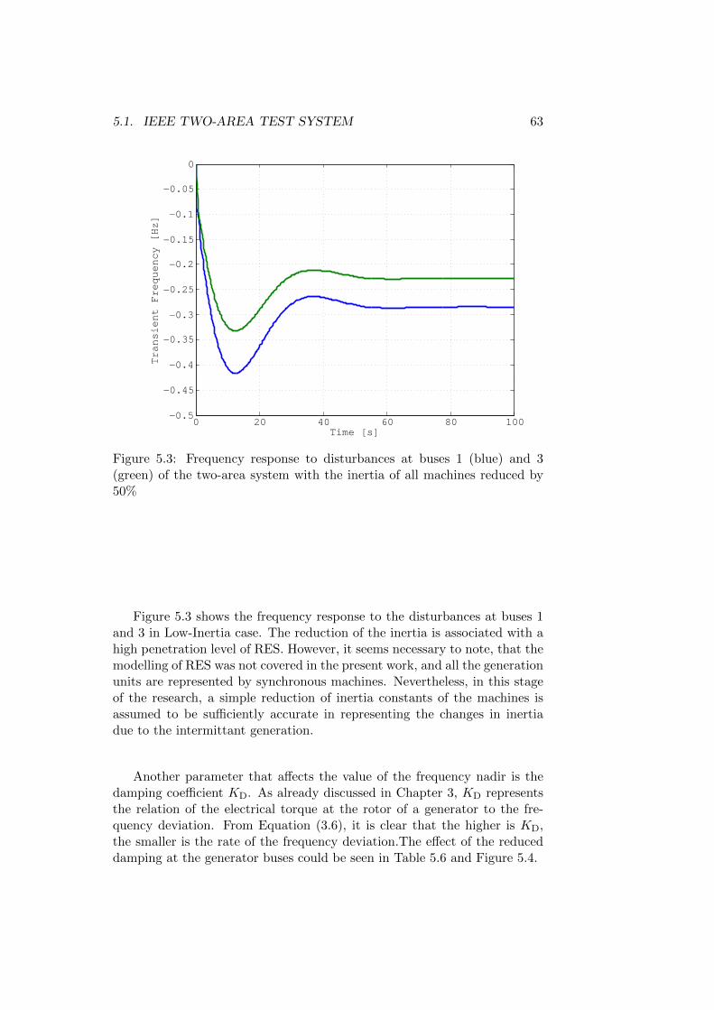
5.1. IEEE TWO-AREA TEST SYSTEM 63
0 20 40 60 80 100−0.5
−0.45
−0.4
−0.35
−0.3
−0.25
−0.2
−0.15
−0.1
−0.05
0
Time [s]
Tra
nsi
en
t F
req
ue
ncy
[H
z]
Figure 5.3: Frequency response to disturbances at buses 1 (blue) and 3(green) of the two-area system with the inertia of all machines reduced by50%
Figure 5.3 shows the frequency response to the disturbances at buses 1and 3 in Low-Inertia case. The reduction of the inertia is associated with ahigh penetration level of RES. However, it seems necessary to note, that themodelling of RES was not covered in the present work, and all the generationunits are represented by synchronous machines. Nevertheless, in this stageof the research, a simple reduction of inertia constants of the machines isassumed to be sufficiently accurate in representing the changes in inertiadue to the intermittant generation.
Another parameter that affects the value of the frequency nadir is thedamping coefficient KD. As already discussed in Chapter 3, KD representsthe relation of the electrical torque at the rotor of a generator to the fre-quency deviation. From Equation (3.6), it is clear that the higher is KD,the smaller is the rate of the frequency deviation.The effect of the reduceddamping at the generator buses could be seen in Table 5.6 and Figure 5.4.

64 CHAPTER 5. SIMULATION RESULTS
Table 5.6: Results of transient overshoot computation in the two-area systemwith the damping of all the machines reduced by 50%
Node Mminp [Hz] min y(t) [Hz]
1 -0.388 -0.4382 -0.388 -0.4383 -0.310 -0.3484 -0.308 -0.342
0 20 40 60 80 100−0.5
−0.45
−0.4
−0.35
−0.3
−0.25
−0.2
−0.15
−0.1
−0.05
0
Time [s]
Tra
nsi
en
t F
req
ue
ncy
[H
z]
Figure 5.4: Frequency response to disturbances at buses 1 (blue) and 3(green) of the two-area system with damping of all the machines reduced by50%
If both the rotational inertia and damping coefficients of the machines arereduced by 50% compared to Base Case, the absolute value of the transientfrequency overshoot increases by 15-17%, as shown in Table 5.7.
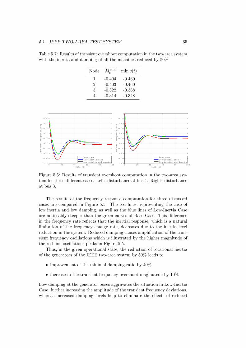
5.1. IEEE TWO-AREA TEST SYSTEM 65
Table 5.7: Results of transient overshoot computation in the two-area systemwith the inertia and damping of all the machines reduced by 50%
Node Mminp min y(t)
1 -0.404 -0.4602 -0.403 -0.4603 -0.322 -0.3684 -0.314 -0.348
0 20 40 60 80 100−0.5
−0.45
−0.4
−0.35
−0.3
−0.25
−0.2
−0.15
−0.1
−0.05
0
Time [s]
Tra
nsi
en
t F
req
ue
ncy
[H
z]
base caselow−inertia caselow inertia and damping
0 20 40 60 80 100−0.5
−0.45
−0.4
−0.35
−0.3
−0.25
−0.2
−0.15
−0.1
−0.05
0
Time [s]
Tra
nsi
en
t F
req
ue
ncy
[H
z]
base caselow−inertia caselow inertia and damping
Figure 5.5: Results of transient overshoot computation in the two-area sys-tem for three different cases. Left: disturbance at bus 1. Right: disturbanceat bus 3.
The results of the frequency response computation for three discussedcases are compared in Figure 5.5. The red lines, representing the case oflow inertia and low damping, as well as the blue lines of Low-Inertia Caseare noticeably steeper than the green curves of Base Case. This differencein the frequency rate reflects that the inertial response, which is a naturallimitation of the frequency change rate, decreases due to the inertia levelreduction in the system. Reduced damping causes amplification of the tran-sient frequency oscillations which is illustrated by the higher magnitude ofthe red line oscillations peaks in Figure 5.5.
Thus, in the given operational state, the reduction of rotational inertiaof the generators of the IEEE two-area system by 50% leads to
• improvement of the minimal damping ratio by 40%
• increase in the transient frequency overshoot maginutede by 10%
Low damping at the generator buses aggravates the situation in Low-InertiaCase, further increasing the amplitude of the transient frequency deviations,whereas increased damping levels help to eliminate the effects of reduced

66 CHAPTER 5. SIMULATION RESULTS
inertia on the transient frequency. For instance, a 40% increase in dampingcoefficients in Low-Inertia case allows to fully mitigate the effect of the 50%inertia reduction on the frequency nadir.
The proposed optimization program has been used to further investigatethe impact of inertia and damping changes on the parameters of interestand to find the optimal levels of inertia and damping.

5.1. IEEE TWO-AREA TEST SYSTEM 67
5.1.3 Optimization
The optimization of inertia and damping in the two-area system has beenaccomplished in several stages on a “simple-to-complex” basis. The parame-ters of the optimization in the investigated cases are presented in Tables 5.8and 5.9.
Table 5.8: Parameters of the optimization program for two-area test system(Case 1 - Case 4)
Parameter Case 1 Case 2 Case 3 Case 4
Kminj 0.25Kbase
j - - -
Mminj 0.25Mbase
j 0.25Mbasej 0.25Mbase
j 0.25Mbasej
Kmaxj 4Kbase
j - - -
Mmaxj 4Mbase
j 4Mbasej 4Mbase
j 2Mbasej
Ktot∑j∈K
Kmaxj - - -
M tot∑j∈M
Mmaxj
∑j∈M
Mmaxj
∑j∈M
Mmaxj
∑j∈M
Mmaxj
cζ 100 100 100 100cKj 0 0 0 0cMj 0 0 0 0cε 0 0 0 0
fp [Hz] - - -0.312 -0.312
Table 5.9: Parameters of the optimization program for two-area test system(Case 5 - Case 8)
Parameter Case 5 Case 6 Case 7 Case 8
Kminj - 0.25Kbase
j 0.25Kbasej 0.25K low inert.
j
Mminj 0.25Mbase
j 0.25Mbasej 0.25Mbase
j 0.25M low inert.j
Kmaxj - 4Kbase
j 4Kbasej 4K low inert.
j
Mmaxj 4Mbase
j 4Mbasej 4Mbase
j 4M low inert.j
Ktot -∑j∈K
Kmaxj
∑j∈K
Kmaxj
∑j∈K
Kmaxj
M tot∑j∈M
Mmaxj
∑j∈M
Mmaxj
∑j∈M
Mmaxj
∑j∈M
Mmaxj
cζ 100 100 100 100cKj 0 0 0.01 0.01cMj 0.015 0.015 0.015 0.015cε 0 0 0 15
fp [Hz] -0.312 -0.312 -0.312 -0.312

68 CHAPTER 5. SIMULATION RESULTS
Case 1 In Case 1, the minimal damping ratio was optimized withoutputting a constraint on the frequency overshoot. Furthermore, the costsof inertia and damping procurement were set to zero. The results of thissimplified optimization case could serve as a validation of the general per-formance of the algorithm.
By means of the developed optimization program, the minimal dampingratio in Case 1 was increased by 94% compared to Base Case. The optimiza-tion results are summarized in Table 5.10 and Table 5.11. The inertia con-stants were significantly reduced compared to Base Case, whereas the damp-ing coefficients were increased to the maximal possible values. This outcomemeets all the expectations and conforms with the findings of Low-Inertia caseanalysis (Table 5.3). It should be noted, that the inertia constants M didnot reach the minimal values Mmin
j = 0.25Mbasej . A simple computation of
the eigenvalues with Mminj = 0.25Mbase
j yields ζmin = 0.3378, showing thata further reduction of M from the values listed in Table 5.11 does not lead tothe enhancement of the minimal damping ratio. The changes in inertia anddamping that improve the damping ratio of one oscillatory mode may causea significant reduction of another damping ratio. Therefore, at some point,a further enhancement of the minimal damping ratio becomes impossible,since there are several damping ratios that compete with each other. Thus,it can be concluded that the optimization program has successfully foundthe optimal solution of Case 1.
Table 5.10: Optimization results of the two-area test system (Case 1)
ζmin0 0.2074ζmin
opt 0.4024
Number of Iterations 90Improvement 94%Mmin
p , [Hz] -0.258
Table 5.11: Values of the inertia constants M and damping coefficients KD
on 900 MVA base in the two-area test system (Case 1)
Generator M [s] M/Mbase KD
G1 3.2500 0.25 4G2 4.6222 0.34 4G3 3.1435 0.25 4G4 4.7548 0.38 4
The results of Case 1 implicate that a high share of RES should be seenas a positive condition for the stability of the two-area test system with
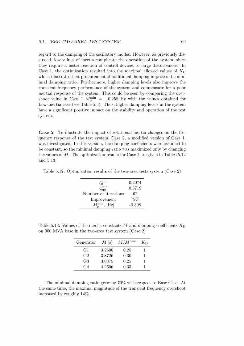
5.1. IEEE TWO-AREA TEST SYSTEM 69
regard to the damping of the oscillatory modes. However, as previously dis-cussed, low values of inertia complicate the operation of the system, sincethey require a faster reaction of control devices to large disturbances. InCase 1, the optimization resulted into the maximal allowed values of KD
which illustrates that procurement of additional damping improves the min-imal damping ratio. Furthermore, higher damping levels also improve thetransient frequency performance of the system and compensate for a poorinertial response of the system. This could be seen by comparing the over-shoot value in Case 1 Mmin
p = −0.258 Hz with the values obtained forLow-Inertia case (see Table 5.5). Thus, higher damping levels in the systemhave a significant positive impact on the stability and operation of the testsystem.
Case 2 To illustrate the impact of rotational inertia changes on the fre-quency response of the test system, Case 2, a modified version of Case 1,was investigated. In this version, the damping coefficients were assumed tobe constant, so the minimal damping ratio was maximized only by changingthe values of M . The optimization results for Case 2 are given in Tables 5.12and 5.13.
Table 5.12: Optimization results of the two-area tests system (Case 2)
ζmin0 0.2074ζmin
opt 0.3719
Number of Iterations 62Improvement 79%Mmin
p , [Hz] -0.398
Table 5.13: Values of the inertia constants M and damping coefficients KD
on 900 MVA base in the two-area test system (Case 2)
Generator M [s] M/Mbase KD
G1 3.2500 0.25 1G2 3.8726 0.30 1G3 3.0875 0.25 1G4 4.2606 0.35 1
The minimal damping ratio grew by 79% with respect to Base Case. Atthe same time, the maximal magnitude of the transient frequency overshootincreased by roughly 14%.

70 CHAPTER 5. SIMULATION RESULTS
Case 3 The limitation of the overshoot magnitude is first considered inCase 3, where the frequency overshoot constraint (4.93), ignored in Case 1and Case 2, was activated. The damping level is kept constant in Case 3to enable the investigation of the inertia impact on the frequency response.The absolute value of |fp| = 0.312 Hz was chosen, which is smaller than0.348 Hz, obtained in Base Case, but larger than 0.258 Hz of Case 1.
Table 5.14: Optimization results of the two-area test system (Case 3)
ζmin0 0.2074ζmin
opt 0.4030
Number of Iterations 61Improvement 94%Mmin
p , [Hz] -0.294
Table 5.15: Values of the inertia constants M and damping coefficients KD
on 900 MVA base in the two-area test system (Case 3)
Generator M [s] M/Mbase KD
G1 49.1459 3.78 1G2 7.3904 0.57 1G3 3.1622 0.26 1G4 4.8596 0.39 1
It should be noted, that the 94% improvement, obtained in Case 3,repeats the result of Case 1. However, in Case 3, the damping coefficientsremained at their initial level KD = 1, whereas in Case 1 their maximizationsignificantly enhances the minimal damping ratio, as it could be seen incomparison to Case 2. It could be concluded, that the introduction of thefrequency overshoot constraint pushes the solution of the highly nonlinearproblem into another direction of the solving.
The results, presented in Tables 5.14 and 5.15, show that in order tokeep the transient frequency in the acceptable range while maximizing thedamping ratio, the program suggests to significantly increase the rotationalinertia at bus 1.
First of all, the results of Case 3 indicate a high participation of the G1states in the dominating oscillatory mode. Furthermore, as it could be seenin Tables 5.5-5.7, the frequency overshoot at buses 1 and 2 has a greatermagnitude than at nodes 3 and 4, hence, it is more likely for the frequencyof G1 or G2 to violate the overshoot constraint.

5.1. IEEE TWO-AREA TEST SYSTEM 71
Case 4 To check how the availability of inertia at bus 1 affects the opti-mal solution, Case 4 was designed, with the total available inertia at bus 1reduced by 50% to 2Mbase
1 . The results of the Case 4 simulations can befound in Tables 5.16 and 5.17.
Table 5.16: Optimization results of the two-area test system (Case 4)
ζmin0 0.2074ζmin
opt 0.2829
Number of Iterations 47Improvement 36%Mmin
p , [Hz] -0.312
Table 5.17: Values of the inertia constants M and damping coefficients KD
on 900 MVA base in the two-area test system (Case 4)
Generator M [s] M/Mbase KD
G1 26.0000 2.00 1G2 12.6602 0.97 1G3 5.4356 0.42 1G4 7.8022 0.60 1
The restriction imposed on the bus 1 inertia reserves reduces the im-provement of the minimal damping ratio from 94% to 36%. The solutionis obtained by deploying the whole available inertia reserve at bus 1 andreducing the rotational inertia at buses 3 and 4.
Case 5 Another possibility to limit the inertia changes is to impose thecosts on each additional inertia unit. In the developed program, it is assumedthat both reduction and increase of the inertia could be regarded as a serviceand could be rated with the same costs.
In Case 5, the damping at the generator buses remains unchanged,whereas the rotational inertia changes are penalized with cMj = 0.015.The transient frequency overshoot is restricted at the same level as before,fp = −0.312 Hz.

72 CHAPTER 5. SIMULATION RESULTS
Table 5.18: Optimization results of the two-area test system (Case 5)
ζmin0 0.2074ζmin
opt 0.3832
Number of Iterations 54Improvement 85%Mmin
p , [Hz] -0.312
Table 5.19: Values of the inertia constants M and damping coefficients KD
on 900 MVA base in the two-area test system (Case 5)
Generator M [s] M/Mbase KD
G1 34.0543 2.62 1G2 12.9336 1.00 1G3 3.0875 0.25 1G4 4.4721 0.35 1
The obtained results (see Tables 5.18 and 5.19) are similar to those ofCase 4. The inertia of G1 is increased by 162%, while it is set to the minimalvalue at bus 3 and close to the minimal value at bus 4. However, the inertialevel at bus 2 remains intact which can be seen as a reaction to the costsimposed on the changes.
Case 6 Case 6 illustrates the optimization of both inertia and dampingunder the same conditions as in Case 5. The damping changes, in contrastto the inertia changes, are not penalized by costs in this case. The resultsin Tables 5.20 and 5.21 show that by setting the damping at the maximalvalues, the improvement level of 86% can be achieved, which is close tothe performance of the program in Case 1. At the same time, the requiredadjustments of inertia in Case 6 are much smaller than in Case 1. Thisdiscrepancy draws attention to the important role of the damping for thestability of the investigated two-area test system.
Table 5.20: Optimization results of the two-area test system (Case 6)
ζmin0 0.2075ζmin
opt 0.3796
Number of Iterations 88Improvement 83%Mmin
p , [Hz] -0.252
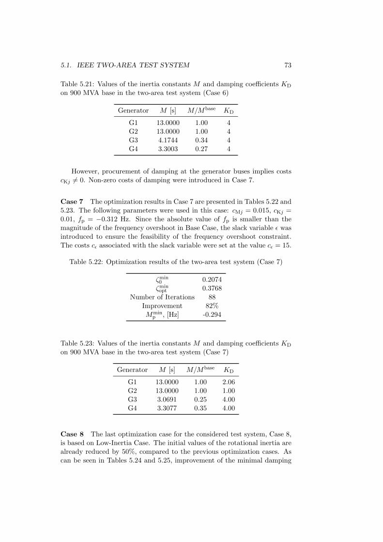
5.1. IEEE TWO-AREA TEST SYSTEM 73
Table 5.21: Values of the inertia constants M and damping coefficients KD
on 900 MVA base in the two-area test system (Case 6)
Generator M [s] M/Mbase KD
G1 13.0000 1.00 4G2 13.0000 1.00 4G3 4.1744 0.34 4G4 3.3003 0.27 4
However, procurement of damping at the generator buses implies costscKj 6= 0. Non-zero costs of damping were introduced in Case 7.
Case 7 The optimization results in Case 7 are presented in Tables 5.22 and5.23. The following parameters were used in this case: cMj = 0.015, cKj =0.01, fp = −0.312 Hz. Since the absolute value of fp is smaller than themagnitude of the frequency overshoot in Base Case, the slack variable ε wasintroduced to ensure the feasibility of the frequency overshoot constraint.The costs cε associated with the slack variable were set at the value cε = 15.
Table 5.22: Optimization results of the two-area test system (Case 7)
ζmin0 0.2074ζmin
opt 0.3768
Number of Iterations 88Improvement 82%Mmin
p , [Hz] -0.294
Table 5.23: Values of the inertia constants M and damping coefficients KD
on 900 MVA base in the two-area test system (Case 7)
Generator M [s] M/Mbase KD
G1 13.0000 1.00 2.06G2 13.0000 1.00 1.00G3 3.0691 0.25 4.00G4 3.3077 0.35 4.00
Case 8 The last optimization case for the considered test system, Case 8,is based on Low-Inertia Case. The initial values of the rotational inertia arealready reduced by 50%, compared to the previous optimization cases. Ascan be seen in Tables 5.24 and 5.25, improvement of the minimal damping

74 CHAPTER 5. SIMULATION RESULTS
ratio is achieved by a further reduction of the rotational inertia, and thefrequency overshoot constraint is satisfied by increased damping levels.
Table 5.24: Optimization results of the two-area test system (Case 8)
ζmin0 0.2926ζmin
opt 0.3840
Number of Iterations 190Improvement 38%Mmin
p , [Hz] -0.312
Table 5.25: Values of the inertia constants M and damping coefficients KD
on 900 MVA base in the two-area test system (Case 8)
Generator M [s] M/M low inert KD
G1 3.4298 0.53 2.14G2 4.0404 0.62 2.14G3 2.9882 0.46 2.14G4 4.4418 1.68 2.14
5.1.4 Transient Stability Analysis
The results obtained for the two-area test system by means of the optimiza-tion program could be illustrated by the results of the transient simulationsimplemented in MATLAB. The developed transient simulation program al-lows to observe the behaviour of the system state variables after large sym-metrical disturbances. One of the disturbances of interest is a three-phaseshort circuit at one of the circuits of the line 8-9 close to bus 9. Such adisturbance can be classified as an overfrequency event, since it leads to theacceleration of the synchronous machines due to reduction of the electricaltorque at their rotors. The fault is cleared after 0.01 s by a disconnectionof the faulty circuit. The disconnection of the circuit changes the topologyof the system and decreases the transmission capacity between two areas.The frequency of the generators rises, while the PFCs with Tt = 10s aregradually adjusting the mechanical torque. After a sufficient deployment ofthe primary control reserves is achieved, the frequency decreases and settlesat a new steady value.
As shown previously, inertia and damping in the test system influence onthe transient response of the system. The results of the simulations of thediscussed disturbance conform with this statement. Figure 5.6 illustrates thetransient frequency of G1 after the disturbance of interest in 5 different cases.The presented cases can be divided in two groups, namely the ones with

5.1. IEEE TWO-AREA TEST SYSTEM 75
KDj = 1 (Base Case, Low-Inertia Case, Case 2) and those with improveddamping KDj = 4 (Low Inertia and Low Damping, Case 1). The peaks ofthe first group lines lay considerably higher than those of the second grouplines. This stands as a clear illustration of the influence of damping on thetransient frequency in the investigated system.
0 5 10 15 20 25 30 35 400
0.02
0.04
0.06
0.08
0.1
0.12
0.14
0.16
0.18
Time [s]
Tra
nsi
en
t F
req
ue
ncy
[H
z]
base caselow−inertia caselow inertia and high dampingcase 1case 2
Figure 5.6: Transient frequency of G1 after a short cirtcuit at bus 9 anddisconnection of a circuit of the line 8-9 of the two-area test system
Among the cases of the first group, Base Case implicates the highest val-ues of the rotational inertia and, thus, demonstrates the strongest inertialresponse. Therefore, as illustrated by the blue line in the graph, Base Case isassociated with the slowest rise and the smallest magnitude of the transientfrequency compared to the other cases in the group. Case 2, character-ized by very low levels of inertia and an improved minimal damping ratio,demonstrates the highest rate and magnitude of the frequency deviation.However, the difference between the peak values of the transient frequencyin Base Case and Case 2 is merely 0.01 Hz which is 6.25% of the magnitudein Base Case.
Figure 5.6 does not give a clear impression on the transients occuringright after the short circuit. The transient frequency within the first 5seconds after the fault is shown in Figure 5.7. This graph demonstrates thatthe lower is the inertia, the steeper is the growth of the frequency after the

76 CHAPTER 5. SIMULATION RESULTS
disturbance. In this case, the rate of the frequency change is independentfrom the damping in the system. Thus, the inertial response of the system,along with the initial state of the system and severeness of the disturbance,define how much time the protection systems have to clear the fault beforethe system stability is lost.
0 1 2 3 4 50
0.02
0.04
0.06
0.08
0.1
0.12
Time [s]
Tra
nsi
en
t F
req
ue
ncy
[H
z]
base caselow−inertia caselow inertia and high dampingcase 1case 2
Figure 5.7: Transient frequency of G1 after a short cirtcuit at bus 9 anddisconnection of a circuit of the line 8-9 of the two-area test system (first 5seconds)
The effect of the inertial response on the critical fault clearing time canbe observed by comparing two plots in Figure 5.8. Both plots represent therotor angles of the four generators after the considered disturbance. Thefault was cleared in both cases after 0.012 s, but the rotational inertia of thegenerators in the left graph was set to the values of Base Case, whereas atthe right, the same event within Low-Inertia Case is modelled. With inertiavalues of Base Case, the system remains stable. In contrast, in Low-InertiaCase, the generators G3 and G4 fall out of step, which implicates islandingof the two areas.

5.2. IEEE SOUTH EAST AUSTRALIAN TEST SYSTEM 77
0 10 20 30 40 50 60 70 80−0.6
−0.4
−0.2
0
0.2
0.4
0.6
0.8
Time [s]
Re
lativ
e R
oto
r A
ng
le [ra
d]
G1G2G3G4
0 10 20 30 40 50 60 70 80−1000
0
1000
2000
3000
4000
5000
6000
7000
8000
Time [s]
Re
lativ
e R
oto
r A
ng
le [ra
d]
G1G2G3G4
Figure 5.8: Rotor angles of the generators G1-G4 of the two-area test systemafter a short circuit at bus 9 in Base Case (left) and Low-Inertia Case (right)
5.2 IEEE South East Australian Test System
5.2.1 System Description
A simplified 14-generator test system, based on the southern and easternAustralian power networks, is shown in Figure E.1. It consists of 5 areas,with areas 1 and 2 more closely electrically coupled. This test system willbe further reffered to as the five-area test system. The system is charac-terized by its long tie lines and, according to [4], demonstrates 3 inter-areaoscillatory modes and 10 local-area modes, with some of these modes beingunstable without PSSs. The parameters of the grid elements and the powerflow data are adopted from [4]. The initial steady-state operating conditionof the system corresponds to the case 2 (medium-heavy loading) of [4].
The parameters of the grid and the detailed power flow data are pre-sented in Appendix E. The parameters of the PFCs repeat those of thetwo-area system. It should be noted, that the types and models of AVR andPSS used in the present thesis (see Chapter 2) differ from those implementedby the authors of [4]. Modelling of SVC is not included in the present work,therefore, all the SVCs were represented by uncontrolled reactive shunts.Furthermore, some of the generator parameters, listed in Table E.3, such assaturation constants, were approximated by using the typical data from [2]and [19], since they are not given in [4]. Due to the mentioned discrepanciesin the modelling, benchmarking of the results presented in this thesis withthose of [4] is not possible.
The initial operating condition of the investigated system is described inTable 5.26. Power flow occurs from south (Area 5) to north (Area 4).

78 CHAPTER 5. SIMULATION RESULTS
Table 5.26: Steady-state operating condition of the five-area test system
Load Condition Medium-HeavyTotal generation [MW] 21590
Total load [MW] 21000
Inter-area flows
Area 4 to Area 2 [MW] -500Area 2 to Area 1 [MW] -1120Area 1 to Area 3 [MW] -1000Area 3 to Area 5 [MW] -500
5.2.2 Small-Signal Stability Analysis
Similarly as in case of the two-area test system, the analysis of the small-signal stability of the five-area test system starts with calculation of theeigenvalues of the system matrix in Base Case and Low-Inertia Case. Com-plete lists of the eigenvalues in the two considered cases can be found inAppendix E.
The values of M and KD used in the two cases are presented in Ta-ble 5.27. The parameters are given on 100 MVA base to conform with thep.u. base of the data in Appendix E. The values of KD in Table 5.27 cor-respond to KD = 1 on rated power of the generators. In Base Case, the
Table 5.27: Rotational inertia constants M and damping coefficients of thefive-area test system generators in Base Case and Low-Inertia Case, calcu-lated on 100 MVA base
Generator G1 G2 G3 G4 G5 G6 G7
Node 101 201 202 203 204 301 302KD 9.999 33.335 22.224 16.668 26.668 53.336 17.776
M Base [s] 71.993 213.344 124.454 106.675 138.674 298.682 124.432M Low Inertia [s] 35.996 106.672 62.227 53.338 69.337 149.341 62.216
Generator G8 G9 G10 G11 G12 G13 G14
Node 401 402 403 404 501 502 503KD 17.776 9.999 17.776 19.998 6.666 10.000 8.335
M Base [s] 106.656 79.992 92.435 103.990 46.662 80.000 125.025M Low Inertia [s] 53.328 39.996 46.218 51.995 23.331 40.000 62.513
five-area system has a very low minimal damping ratio, ζminbase = 0.096, as
could be seen in Table E.4. Furthermore, the system exhibits three moreoscillatory modes with damping ratios lower than 0.200. Thus, oscillationsoccuring after small disturbances in this system decay at a very slow rate,and changes of the operating state of the system might lead to its instability.
In Low-Inertia Case, the system is unstable with an expanding oscillatory

5.2. IEEE SOUTH EAST AUSTRALIAN TEST SYSTEM 79
mode λ = 1.812 ± 39.368 (see Table E.5). This might cause considerableconcerns, if the system has a high installed capacity of RES.
Frequency response of the five-area test system was estimated in thesame way as it was done for the two-area system, i.e. by applying steplikeload changes to the generator buses. The results of the transient overshootapproximation are shown in Table 5.28. The magnitude of the overshootdepends on the node where disturbance occured. As could be seen in Ta-ble 5.28, disturbances that take place in the same area cause frequencydeviations of the same amplitude. The magnitude of the overshoot has thehighest value in Area 5 and decreases in accordance with the power flowdirection.
Table 5.28: Results of transient overshoot computation in the five-area testsystem in Base Case
Node Generator Mminp [Hz] Node Generator Mmin
p [Hz]
101 G1 -0.040 401 G8 -0.032201 G2 -0.040 402 G9 -0.035202 G3 -0.040 403 G10 -0.035203 G4 -0.040 404 G11 -0.035204 G5 -0.040 501 G12 -0.050301 G6 -0.049 502 G13 -0.052302 G7 -0.047 503 G14 -0.052

80 CHAPTER 5. SIMULATION RESULTS
5.2.3 Optimization
Poor damping of oscillatory modes in the five-area system can be improvedby providing synthetical inertia and additional damping. By means of thedeveloped optimization program, the required amount of inertia and damp-ing at the generator nodes can be estimated.
The optimization was carried out for three cases with different parame-ters presented in Table 5.29.
Table 5.29: Parameters of the optimization program for the five-area testsystem
Parameter Case 1 Case 2 Case 3
Kminj 0.25Kbase
j 0.25Kbasej 0.25Kbase
j
Mminj 0.25Mbase
j 0.25Mbasej 0.25Mbase
j
Kmaxj 4Kbase
j 4Kbasej 4Kbase
j
Mmaxj 4Mbase
j 4Mbasej 4Mbase
j
cζ 100 100 100cKj 0 0.001 0.001cMj 0 0.015 0.015cε 0 0 15
fp [Hz] - - -0.045
Case 1 In Case 1, costs of inertia and damping provision were set tozero, and the frequency overshoot was not constrained. The results of theoptimization in Case 1 are shown in Tables 5.30 and 5.31. The developedprogram allows to improve the minimal damping ratio by 82%. Any furtherimprovement of the initially lowest damping ratio leads to a decrease inanother critical damping ratio which limits the possible advances of thealgorithm.
To achieve an 82% improvement of the minimal damping ratio, the rota-tional inertia at five buses was reduced, whereas at the rest of the nodes, itwas increased, with the maximal value of 3.62Mbase at G12. Furthermore,adjusted values of damping at majority of the buses are lower than thosein Base Case. Only the damping values of the generators in Area 5 aresignificantly increased.

5.2. IEEE SOUTH EAST AUSTRALIAN TEST SYSTEM 81
Table 5.30: Optimization results of the five-area test system (Case 1)
ζmin0 0.0960ζmin
opt 0.1743
Number of Iterations 185Improvement 82%Mmin
p , [Hz] -0.047
Table 5.31: Values of the inertia constants M and damping coefficients KD
on 100 MVA base in the five-area test system (Case 1)
Generator M [s] M/Mbase KD KD/KbaseD
G1 30.06 0.42 8.82 0.88G2 500.74 2.35 27.07 0.81G3 257.49 2.07 11.14 0.50G4 183.60 1.72 20.77 1.25G5 311.87 2.25 13.34 0.50G6 193.20 0.65 26.70 0.50G7 172.32 1.38 13.58 0.76G8 155.43 1.46 13.65 0.77G9 52.79 0.66 5.03 0.50G10 39.10 0.42 16.98 0.96G11 114.45 1.10 10.06 0.50G12 169.12 3.62 23.75 3.56G13 72.55 0.91 34.20 3.42G14 149.22 1.19 28.65 3.44
Case 2 In Case 2, changes of inertia and damping are penalized by costscMj = 0.015 and cKj = 0.01, respectively. As shown in Tables 5.32 and 5.33,introduction of the costs significantly affects the optimization results. Incontrast to Case 1, inertia is changed only at two generators in Area 2, G2and G4, and two generators in Area 5, G12 and G14. The values of inertia ofthe corresponding aggregated machines are increased, furthermore, dampingof G2 and G12 is considerably higher than in Base Case. Inertia and damp-ing at the rest of nodes stay intact. From the results of Case 1 and Case 2,it could be concluded that generators G2, G4, G12, and G14 participate themost in the critical oscillatory modes. However, the obtained results do notconform with the expectation that damping ratios are improved by inertiareduction.

82 CHAPTER 5. SIMULATION RESULTS
Table 5.32: Optimization results for the five-area test system (Case 2)
ζmin0 0.0960ζmin
opt 0.1511
Number of Iterations 150Improvement 58%Mmin
p , [Hz] -0.049
Table 5.33: Values of the inertia constants M and damping coefficients KD
on 100 MVA base in the five-area test system (Case 2)
Generator M [s] M/Mbase KD KD/KbaseD
G1 71.99 1.00 10.00 1.00G2 319.95 1.50 71.73 2.15G3 124.45 1.00 22.22 1.00G4 115.53 1.08 16.67 1.00G5 138.67 1.00 26.67 1.00G6 298.68 1.00 53.34 1.00G7 124.43 1.00 17.78 1.00G8 106.66 1.00 17.78 1.00G9 79.99 1.00 10.00 1.00G10 92.44 1.00 17.78 1.00G11 103.99 1.00 20.00 1.00G12 123.20 2.64 17.50 2.63G13 80.00 1.00 10.00 1.00G14 141.52 1.13 8.34 1.00
Case 3 Optimization under the frequency overshoot constraint was con-sidered in Case 3. The threshold fp was set to -0.045 Hz. The optimizationresults for Case 3 are presented in Tables 5.34 and 5.35. Inertia and damp-ing of generator G12 are significantly increased compared with Case 2. Theoptimization of inertia and damping levels in the five-area system with con-strained transient frequency allowed to improve the minimal damping ratioof the system by 66%.
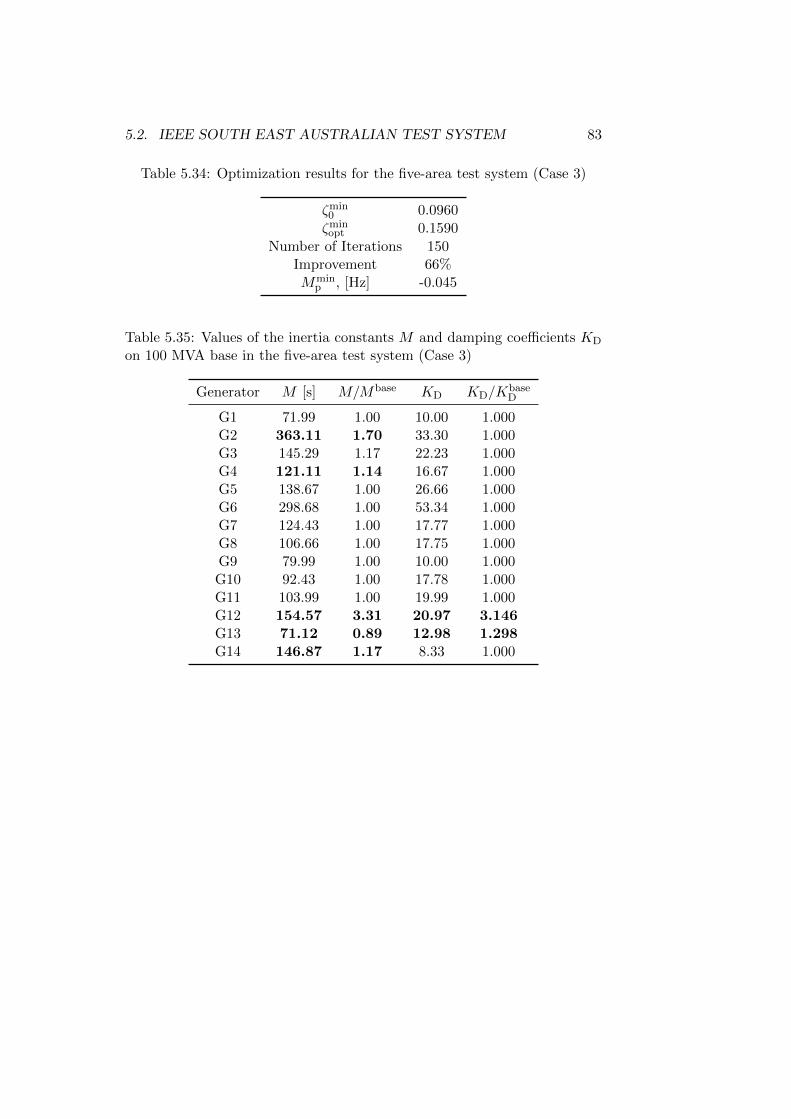
5.2. IEEE SOUTH EAST AUSTRALIAN TEST SYSTEM 83
Table 5.34: Optimization results for the five-area test system (Case 3)
ζmin0 0.0960ζmin
opt 0.1590
Number of Iterations 150Improvement 66%Mmin
p , [Hz] -0.045
Table 5.35: Values of the inertia constants M and damping coefficients KD
on 100 MVA base in the five-area test system (Case 3)
Generator M [s] M/Mbase KD KD/KbaseD
G1 71.99 1.00 10.00 1.000G2 363.11 1.70 33.30 1.000G3 145.29 1.17 22.23 1.000G4 121.11 1.14 16.67 1.000G5 138.67 1.00 26.66 1.000G6 298.68 1.00 53.34 1.000G7 124.43 1.00 17.77 1.000G8 106.66 1.00 17.75 1.000G9 79.99 1.00 10.00 1.000G10 92.43 1.00 17.78 1.000G11 103.99 1.00 19.99 1.000G12 154.57 3.31 20.97 3.146G13 71.12 0.89 12.98 1.298G14 146.87 1.17 8.33 1.000

84 CHAPTER 5. SIMULATION RESULTS
5.2.4 Transient Stability Analysis
In Case 1, rotational inertia of several generators is significantly reduced.This might affect the frequency stability of the system after large distur-bances. For further investigation, a short circuit at bus 217 was modelledby means of the developed transient simulations tool. The short circuit iseliminated after 0.005 s by disconnection of one of the circuits of the line217-215. Thus, the transmisission capacity between Area 1 and Area 2 is re-duced. Figure 5.9 illustrates the resulting rotor angular velocity excursionsin Base Case (left) and Case 1 (right).
0 0.5 1 1.5 2 2.5 3 3.5 4−0.5
0
0.5
1
1.5
2
2.5
3
3.5
4x 10 −4
G1G2G3G4G5G6G7G8G9G10G11G12G13G14
0 0.5 1 1.5 2 2.5 3 3.5 4−0.03
−0.02
−0.01
0
0.01
0.02
0.03
G1G2G3G4G5G6G7G8G9G10G11G12G13G14
Figure 5.9: Rotor angular velocity of the generators of the five-area testsystem after a short circuit at bus 217 and disconnection of a circuit of theline 217-215 in Base Case (left) and Case 1 (right)
Generator G1 has the electrically closest location to the faulty bus. Thefault leads to a large power imbalance at the rotor of this generator, withmechanical power exceeding the power that can be transmitted from thegenerator to other areas or consumed by the load at bus 102. In Case 1,with inertia of G1 reduced by 60%, the disturnance leads to the accelerationof G1 and, consequently, this generator loses synchronism with the grid.This illustrates the importance of the transient frequency restriction for theinertia optimization.
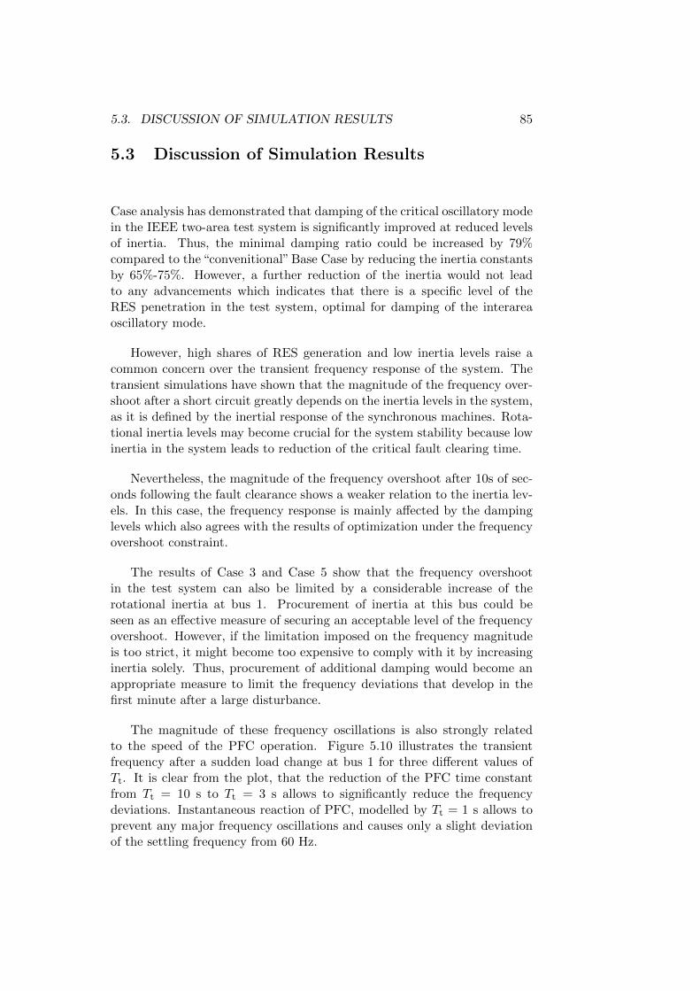
5.3. DISCUSSION OF SIMULATION RESULTS 85
5.3 Discussion of Simulation Results
Case analysis has demonstrated that damping of the critical oscillatory modein the IEEE two-area test system is significantly improved at reduced levelsof inertia. Thus, the minimal damping ratio could be increased by 79%compared to the “convenitional” Base Case by reducing the inertia constantsby 65%-75%. However, a further reduction of the inertia would not leadto any advancements which indicates that there is a specific level of theRES penetration in the test system, optimal for damping of the interareaoscillatory mode.
However, high shares of RES generation and low inertia levels raise acommon concern over the transient frequency response of the system. Thetransient simulations have shown that the magnitude of the frequency over-shoot after a short circuit greatly depends on the inertia levels in the system,as it is defined by the inertial response of the synchronous machines. Rota-tional inertia levels may become crucial for the system stability because lowinertia in the system leads to reduction of the critical fault clearing time.
Nevertheless, the magnitude of the frequency overshoot after 10s of sec-onds following the fault clearance shows a weaker relation to the inertia lev-els. In this case, the frequency response is mainly affected by the dampinglevels which also agrees with the results of optimization under the frequencyovershoot constraint.
The results of Case 3 and Case 5 show that the frequency overshootin the test system can also be limited by a considerable increase of therotational inertia at bus 1. Procurement of inertia at this bus could beseen as an effective measure of securing an acceptable level of the frequencyovershoot. However, if the limitation imposed on the frequency magnitudeis too strict, it might become too expensive to comply with it by increasinginertia solely. Thus, procurement of additional damping would become anappropriate measure to limit the frequency deviations that develop in thefirst minute after a large disturbance.
The magnitude of these frequency oscillations is also strongly relatedto the speed of the PFC operation. Figure 5.10 illustrates the transientfrequency after a sudden load change at bus 1 for three different values ofTt. It is clear from the plot, that the reduction of the PFC time constantfrom Tt = 10 s to Tt = 3 s allows to significantly reduce the frequencydeviations. Instantaneous reaction of PFC, modelled by Tt = 1 s allows toprevent any major frequency oscillations and causes only a slight deviationof the settling frequency from 60 Hz.

86 CHAPTER 5. SIMULATION RESULTS
0 20 40 60 80 100−0.5
−0.45
−0.4
−0.35
−0.3
−0.25
−0.2
−0.15
−0.1
−0.05
0
Time [s]
Tra
nsi
en
t F
req
ue
ncy
[H
z]
Tt = 1s
Tt = 3s
Tt = 10s
Figure 5.10: Transient frequency response to a disturbance in the two-areatest system with different values of the time constant Tt
Such a fast PFC could be provided by BESS [7]. The damping procure-ment might be also accomplished by means of BESS [20]. However, if thestorage systems are used for damping, it requires from them an immedi-ate reaction to any oscillations of the frequency, whereas PFC reserves areactivated outside of a dead-band around the nominal frequency. In Conti-nental Europe, this dead-band is ±10mHz [7]. The potential of the batterysystems in provision of these two services simultaneously should be furtherinvestigated.
IEEE South East Australian test system has demonstrated very poordamping of the oscillatory modes. Improvement of the minimal dampingratio by 82% can be achieved by inertia and damping adjustment. Thesolution implicates increased level of inertia at particular buses which doesnot meet the expectations that high inertia would worsen the damping.Furthermore, in Low-Inertia Case, with inertia constant reduced by 50%,the test system becomes unstable.
The discrepancy between the results and the expectations can be orig-inated in the simplicity of the employed AVR and PSS models and lack oftuning of thier parameters. Alternative models of the control devices were

5.3. DISCUSSION OF SIMULATION RESULTS 87
not implemented due to a different focus of the present work. To furtherimprove the optimization program, various types of AVR and PSS shouldbe added to its modelling capabilities. Nevertheless, the developed programproved to enable the inertia and damping optimization for a more complexpower system than the two-area test system.

88 CHAPTER 5. SIMULATION RESULTS
Chapter 6
Conclusions and outlook
The present work investigated the impact of rotational inertia changes ondamping of oscillatory modes and frequency stability of a power system.The analysis of system stability was based on a multimachine power systemrepresentation with incorporation of a detailed synchronous machine model.This model takes into account the voltage dynamics and includes the effectsof AVR, PSS and PFC operation. Based on the implemented synchronousmachine model, along with the models of the interconnecting transmissionnetwork and aggregated load, a set of system equations was formulated.Linearization of these equations enabled the calculation of the system statematrix and the small-signal stability analysis of a power system.
Further, the sensitivities of the damping ratios of the system oscillatorymodes to inertia and damping were calculated. This allows to evaluatethe changes in the system modes due to incremental changes of inertia anddamping at the system nodes. To assess the frequency dynamics of a powersystem, the magnitude of the transient overshoot in response to a steplikeload change was approximated by using a transfer function. The sensitivitiesof this magnitude to inertia and damping were estimated by computing thesensitivities of the eigenvector product.
The calculated sensitivities were employed in an algorithm for optimiza-tion of inertia and damping. The objective of this algorithm, based on [1], isthe maximization of the minimal damping ratio associated with the systemoscillatory modes. The improvement is achieved by adjusting rotational in-ertia and damping at the system nodes. At the same time, the algorithmallows to limit the magnitude of the transient frequency overshoot whichensures acceptable levels of the frequency deviations in the system. Thechanges of inertia and damping are penalized with costs which serves as asimplified representation of remuneration for provision of synthetic inertiaand additional damping.
The proposed algorithm was implemented in the engineering environ-ment MATLAB. To assess the performance of the developed program, a
89

90 CHAPTER 6. CONCLUSIONS AND OUTLOOK
case study was conducted for two test systems, IEEE two-area test systemand IEEE South East Australian test system. The case analysis of the for-mer system included eight cases with different optimization parameters. Itwas shown, that a reduction of rotational inertia significantly improves thedamping of the oscillatory modes. However, a simultaneous limitation ofthe transient frequency deviations required the provision of additional iner-tia and damping at particular nodes. Introduction of costs for inertia anddamping procurement affected the optimal solution by leaving only the mosteffective changes of inertia and damping. The influence of PFC speed onthe frequency nadir was shown. The impact of inertia on frequency devi-ations after a severe disturbance was illustrated by the results of transientsimulations implemented in MATLAB.
The minimal damping ratio of IEEE South East Australian test systemwas optimized in three different cases. As an optimal solution in case ofnon-zero costs, higher levels of rotational inertia and damping at particularsystem nodes are suggested. However, the modelling accuracy in case ofthis system should be improved by incorporation of realistic models andparameters of AVR and PSS.
Detailed modelling of AVR, PSS, and turbine governors can be proposedas as an objective for the future work. Implementation of the RES modelsis another possible enhancement of the modelling framework. Furthermore,the algorithm could be adjusted to consider the provision of inertia anddamping at buses with no generation.
Another possible field of research is the economical aspects of inertia anddamping procurement. Economical factors clearly have a great influence onthe optimal inertia and damping levels. Furthermore, pricing at potentialinertia-as-a-service markets requires an adequate estimation of the econom-ical losses due to complications in system operation and outages caused bya certain inertia level.
If the focus of analysis is to be shifted from the maximization of thedamping of oscillations to minimization of the transient frequency overshootin a system with low inertia, the optimization program could be adjustedrespectively, by setting the frequency overshoot magnitude as a main ob-jective while restraining the minimal damping ratio. This would allow tooptimize the operation of the system during a high RES penetration withregard to the frequency response. As shown in the case analysis of the IEEEtwo-area test system, with the optimization program focused on the mini-mal damping ratio, the already low inertia levels are proposed to be furtherreduced. To find a proper balance between two objectives, the consequencesof both poor oscillatory mode damping and high frequency overshoot shouldbe evaluated for each particular power system.

Appendix A
Runge-Kutta Methods ofNumerical Integration
R-K methods used for numerical integration in the present work were pro-posed for power system transient simulations in [2]. Depending on thenumber of evaluations of the first derivative in Taylor series solution, R-K methods of different orders could be used for this purpose. In this thesis,the second order R-K method and Gill’s version of the fourth order R-Kmethod were implemented.
Second order R-K method
Consider the first-order differential equation
dx
dt= f(x, t)
with initial condition xn at the moment tn.
The second-order R-K formula for the value of x at the moment t =tn + ∆t is [2]
xn+1 = xn + ∆x = xn +k1 + k2
2(A.1)
where
k1 = f(xn, tn)∆t
k2 = f(xn + k1, tn + ∆t)∆t
(A.2)
Gill’s version of fourth order R-K method
In Gill’s version of the fourth order R-K method, solution of the differ-ential equation is obtained by a four-step approximation of x. Each stage is
91

92 APPENDIX A. RUNGE-KUTTA METHODS
denoted by j = 1, 2, 3, 4 and described by
kj = aj [f(xj−1, t)− bjqj−1]
xj = xj−1 + kj∆t
qj = qj−1 + 3kj − cjf(xj−1, t)
(A.3)
For the first time interval q0 = 0, in further calculations the value of q0 isgiven by q4 of the previous step. The values of a, b, and c are given by
a1 = 1/2,
a3 = 1 +√
0.5,
b1 = 2,
b3 = 1,
c1 = a1,
c3 = a3,
a2 = 1−√
0.5,
a4 = 1/6,
b2 = 1,
b4 = 2,
c2 = a2
c4 = 1/2
Solution at each time step is represented by x4. The advantage of Gill’sversion of fourth order R-K method is minimization of the roundoff errorsachieved by implementation of the q variable. Furthermore, it requires lessstorage capacity than the original R-K methods.

Appendix B
Calculation of Initial SteadyState
Complex voltage and current at the terminals of a synchronous machine inthe initial operational state can be denoted as
Vt = V ejθ
It = Iejγ (B.1)
The initial value of the rotor angle δ can be estimated by [2]
δ = arg(Vt + (Ra + jXqs)It) (B.2)
Further, d-q components of voltage and current can be calculated as
id = Re(Itej(γ−δ+0.5π)) (B.3)
iq = Im(Itej(γ−δ+0.5π)) (B.4)
ed = Re(Vtej(γ−δ+0.5π)) (B.5)
eq = Im(Vtej(γ−δ+0.5π)) (B.6)
Field circuit current and voltage are given by
ifd =eq +Raiq +Xdsid
Xads(B.7)
efd = Rfdifd (B.8)
Efd =Xadu
Rfdefd(B.9)
The mutual flux linkages Ψad and Ψaq are calculated as follows
Ψad = Xads(−id + ifd) (B.10)
Ψaq = −Xaqsiq (B.11)
93

94 APPENDIX B. CALCULATION OF INITIAL STEADY STATE
Initial values of the flux linkages of the rotor circuits are defined by
Ψfd = Ψad +Xfdifd (B.12)
Ψ1d = Xads(ifd − id) (B.13)
Ψ1q = −Xaqsiq (B.14)
Ψ2q = −Xaqsiq (B.15)
The relative rotor angular velocity is equal to zero in a steady state
∆ωr = 0 (B.16)
The excitation quantities are determined as follows
v1 = V (B.17)
v2 = 0 (B.18)
vs = 0 (B.19)
The AVR reference is given by
Vref =Efd
KA+ v1 (B.20)
The mechanical power is not regulated in the initial steady state
∆Pm = 0 (B.21)

Appendix C
Modelling of TransmissionNetwork Elements
Reactive Shunt DevicesReactive shunt devices (shunt capacitors and reactors) can be representedby corresponding shunt admittance ysh
k .
Figure C.1: A shunt connected to bus k [3]
With the sign convention from [3], the current injection from the shuntis defined by
Ishk = −ysh
k Ek (C.1)
where Ek is the complex voltage at bus k.
Transmission Lines and TransformersDepending on the goals of analysis, transmission lines could be modelledby either differential or algebraic equations. Since the network transientsare out of the focus of the present work, an algebraic model, namely thelumped-circuit model of a transmission line, is used (see Figure C.2).
95

96 APPENDIX C. TRANSMISSION NETWORK MODELLING
Figure C.2: Lumped-circuit model of a transmission line [3]
This model is characterized by its series impedance
zkm = rkm + jxkm (C.2)
and shunt admittance
yshkm = gshkm + jbshkm (C.3)
The series admittance of the line model is given by
ykm = z−1km = gkm + jbkm (C.4)
where
gkm =rkm
r2km + x2
km
(C.5)
bkm = − xkmr2km + x2
km
(C.6)
Another π-model, derived in [3], is used to represent transformers. In caseof transformers, the π-model incorporates complex tap ratios
tkm = akmejφkm (C.7)
where akm is the turns ratio. For in-phase transformers, considered in thisthesis, tkm = akm which means that tkm ∈ R.
In [3], a unified branch model for lines, in-phase transformers, and phase-shifting transformers was developed to facilitate the modelling routine. Thismodel is shown in Figure C.3.
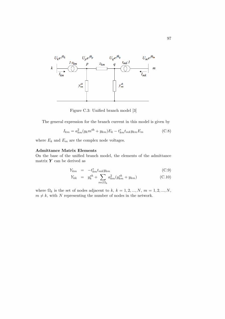
97
Figure C.3: Unified branch model [3]
The general expression for the branch current in this model is given by
Ikm = a2km(ykm
sh + ykm)Ek − t∗kmtmkykmEm (C.8)
where Ek and Em are the complex node voltages.
Admittance Matrix ElementsOn the base of the unified branch model, the elements of the admittancematrix Y can be derived as
Ykm = −t∗kmtmkykm (C.9)
Ykk = yshk +∑m∈Ωk
a2km(yshkm + ykm) (C.10)
where Ωk is the set of nodes adjacent to k, k = 1, 2, ..., N , m = 1, 2, ..., N ,m 6= k, with N representing the number of nodes in the network.

98 APPENDIX C. TRANSMISSION NETWORK MODELLING

Appendix D
Structure of MATLAB inputarrays
Table D.1: Bus data structure (BUSES)
Column Parameter
1 Bus number2 Active power generation [p.u.]3 Reactive power generation [p.u.]4 Active power demand [p.u.]5 Reactive power demand [p.u.]6 Voltage magnitude [p.u.]7 Damping coefficient8 Shunt susceptance [p.u. injected at V=1.0 p.u.]9 Slack bus = 1, Other buses =0
10 Area11 Maximal reactive power [p.u.]12 Minimal reactive power [p.u.]13 Total MVA base of generator [p.u,]14 Maximal active power [p.u.]15 Base Voltage [kV]
99

100 APPENDIX D. STRUCTURE OF MATLAB INPUT ARRAYS
Table D.2: Branch data structure (LINES)
Column Parameter
1 Branch number2 ”From” bus number3 ”To” bus number4 Transformer tap ratio5 Branch resistance [p.u.]6 Branch reactance [p.u.]7 Total line charging susceptance [p.u.]
Table D.3: Generator data structure (GENS)
Row Parameter
1 Aggregated Generator No.2 Node3 Power rating [MVA]4 Inertia constant H [s]5 Number of generators6 Number of generators on-line7 Synchronous reactance Xd [p.u.]8 Synchronous reactance Xq [p.u.]9 Stator leakage inductance Xl [p.u.]
10 Stator resistance Ra [p.u.]11 Transient reactance X ′d [p.u.]12 Transient reactance X ′q [p.u.]
13 Subtransient reactance X ′′d [p.u.]14 Subtransient reactance X ′′q [p.u.]
15 Transient OC time constanct T ′d0 [s]16 Transient OC time constanct T ′q0 [s]
17 Subtransient OC time constant T ′′d0 [s]18 Subtransient OC time constant T ′′q0 [s]
19 Saturation constant Asat
20 Saturation constant Bsat
21 Saturation constant ψt
22 AVR constant KA
23 AVR time constant TR [s]24 PSS constant KSTAB
25 PSS time constant TW [s]26 PSS time constant T1 [s]27 PSS time constant T2 [s]28 Damping coefficient KD
29 Voltage base [kV]

101

102 APPENDIX E. IEEE SOUTH EAST AUSTRALIAN SYSTEM
Appendix E
IEEE South East AustralianSystem
RI-XQHSP 7KH8QLYHUVLW\RI$GHODLGH
)LJXUH 6LPSOLILHGJHQHUDWRU+]V\VWHP
%36B
$69&B
69&
69&
69&
136B
036B
(36B
936B
+36B
569&B
/36B
669&B
369&B
336B
736B
736B
&36B
636B *36B
%69&B
<36B
69&
69&
$5($
$5($
$5($
$5($
$5($
Figure E.1: IEEE South East Australian five-area test system [4]

103
Table E.1: Power flow input data for IEEE South Australian test system [4]calculated on 100 MVA base
Bus No. Pg [p.u.] Qg [p.u.] Pl [p.u.] Ql [p.u.] Vi [p.u.] Qshunt [p.u.] Area Base Voltage [kV]
101 4.788 1.632 0 0 1.000 0 1 15102 0 0 -3.8 -0.38 0 1 330201 28 1.945 0 0 1.000 0 2 20202 19.2 2.42 0 0 1.000 0 2 20203 13.5 2.472 0 0 1.000 0 2 20204 15.84 0.712 0 0 1.000 0 2 20205 0 0.418 -3.3 -0.33 1.055 0 2 330206 0 0 -1.1 -0.11 0 2 330207 0 0 -16 -1.6 0 2 330208 0 0 -1.8 -0.18 0 2 330209 0 0 0 0 0 2 330210 0 0 0 0 0 2 500211 0 0 -14.45 -1.45 0 2 330212 0 0 -14.1 -1.4 1.5 2 330213 0 0 0 0 0 2 500214 0 0 0 0 0 2 330215 0 0 -4.1 -0.4 0 2 330216 0 0 -15.65 -1.55 1.5 2 330217 0 0 -10.7 -1.1 0 2 330301 46.8 11.28 0 0 1.000 0 3 20302 15.32 2.532 0 0 1.000 0 3 20303 0 0 0 0 0 3 500304 0 0 0 0 0 3 500305 0 0 0 0 0 3 500306 0 0 -12.3 -1.23 0 3 500307 0 0 -6.5 -0.65 0 3 500308 0 0 -6.55 -0.66 0 3 500309 0 0 -1.95 -0.2 0 3 330310 0 0 0 0 0 3 330311 0 0 0 0 0 3 330312 0 0 -1.15 -0.12 0 3 220313 0 1.294 -24.05 -2.4 1.015 0 3 220314 0 0 -2.5 -0.25 0 3 220315 0 0 0 0 0 3 275401 14 4.66 0 0 1.000 0 4 20402 8.7 0.942 0 0 1.000 0 4 20403 14 1.888 0 0 1.000 0 4 20404 14.64 2.388 0 0 1.000 0 4 20405 0 0 -12.15 -1.2 0 4 275406 0 0 -9.05 -0.9 0 4 275407 0 0 0 0 0 4 275408 0 0 -1.85 -0.2 0 4 275409 0 0 -3.1 -0.3 0.6 4 275410 0 0 -6.5 -0.65 0 4 275411 0 0 -7 -0.7 0.3 4 275412 0 0.639 -15.35 -1.55 1.000 0 4 275413 0 0 0 0 0 4 275414 0 0 0 0 -0.3 4 330415 0 0 0 0 -0.6 4 330416 0 0 0 0 -0.6 4 330501 6 -0.176 0 0 1.000 0 5 20502 8 2.12 0 0 1.000 0 5 15503 6.9 1.845 0 0 1.000 0 5 15504 0 0 -2 -0.4 -0.9 5 275505 0 0 0 0 0 5 275506 0 0 0 0 0 5 275507 0 0.368 -7.1 -1.4 1.040 0 5 275508 0 0 -5.2 -1.05 0 5 275509 0 0.502 -0.7 -0.15 1.027 0 5 275
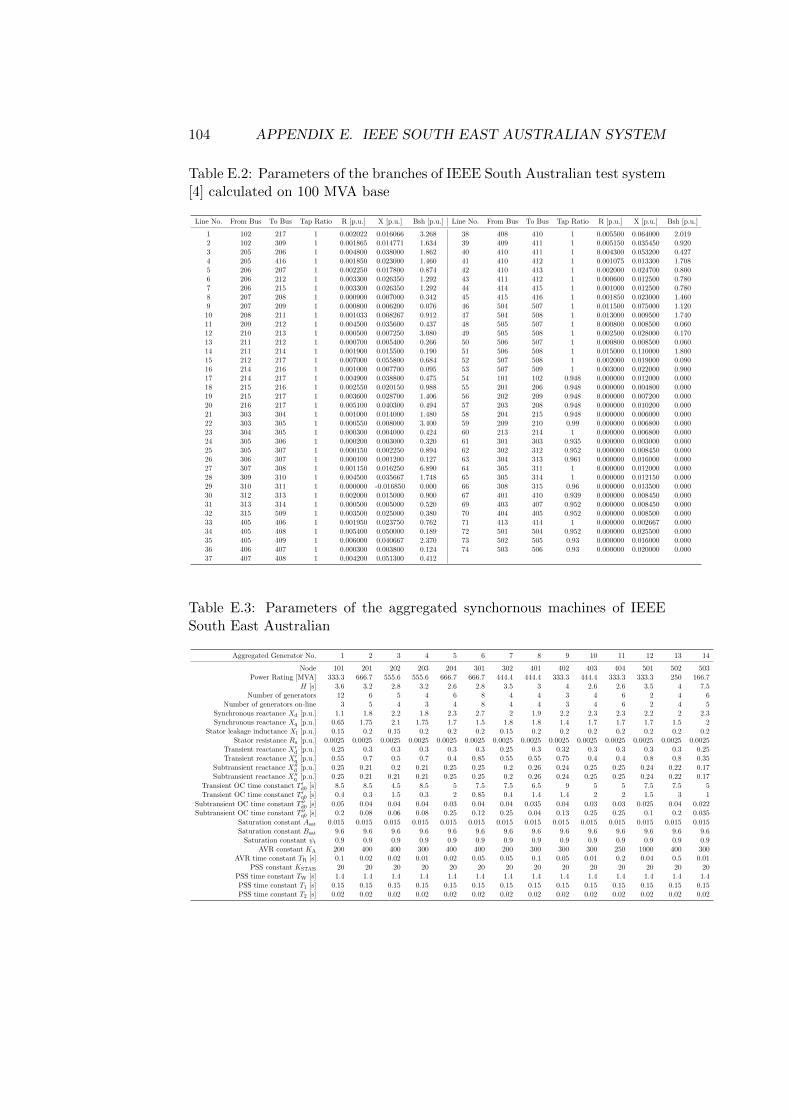
104 APPENDIX E. IEEE SOUTH EAST AUSTRALIAN SYSTEM
Table E.2: Parameters of the branches of IEEE South Australian test system[4] calculated on 100 MVA base
Line No. From Bus To Bus Tap Ratio R [p.u.] X [p.u.] Bsh [p.u.] Line No. From Bus To Bus Tap Ratio R [p.u.] X [p.u.] Bsh [p.u.]
1 102 217 1 0.002022 0.016066 3.268 38 408 410 1 0.005500 0.064000 2.0192 102 309 1 0.001865 0.014771 1.634 39 409 411 1 0.005150 0.035450 0.9203 205 206 1 0.004800 0.038000 1.862 40 410 411 1 0.004300 0.053200 0.4274 205 416 1 0.001850 0.023000 1.460 41 410 412 1 0.001075 0.013300 1.7085 206 207 1 0.002250 0.017800 0.874 42 410 413 1 0.002000 0.024700 0.8006 206 212 1 0.003300 0.026350 1.292 43 411 412 1 0.000600 0.012500 0.7807 206 215 1 0.003300 0.026350 1.292 44 414 415 1 0.001000 0.012500 0.7808 207 208 1 0.000900 0.007000 0.342 45 415 416 1 0.001850 0.023000 1.4609 207 209 1 0.000800 0.006200 0.076 46 504 507 1 0.011500 0.075000 1.12010 208 211 1 0.001033 0.008267 0.912 47 504 508 1 0.013000 0.009500 1.74011 209 212 1 0.004500 0.035600 0.437 48 505 507 1 0.000800 0.008500 0.06012 210 213 1 0.000500 0.007250 3.080 49 505 508 1 0.002500 0.028000 0.17013 211 212 1 0.000700 0.005400 0.266 50 506 507 1 0.000800 0.008500 0.06014 211 214 1 0.001900 0.015500 0.190 51 506 508 1 0.015000 0.110000 1.80015 212 217 1 0.007000 0.055800 0.684 52 507 508 1 0.002000 0.019000 0.09016 214 216 1 0.001000 0.007700 0.095 53 507 509 1 0.003000 0.022000 0.90017 214 217 1 0.004900 0.038800 0.475 54 101 102 0.948 0.000000 0.012000 0.00018 215 216 1 0.002550 0.020150 0.988 55 201 206 0.948 0.000000 0.004800 0.00019 215 217 1 0.003600 0.028700 1.406 56 202 209 0.948 0.000000 0.007200 0.00020 216 217 1 0.005100 0.040300 0.494 57 203 208 0.948 0.000000 0.010200 0.00021 303 304 1 0.001000 0.014000 1.480 58 204 215 0.948 0.000000 0.006000 0.00022 303 305 1 0.000550 0.008000 3.400 59 209 210 0.99 0.000000 0.006800 0.00023 304 305 1 0.000300 0.004000 0.424 60 213 214 1 0.000000 0.006800 0.00024 305 306 1 0.000200 0.003000 0.320 61 301 303 0.935 0.000000 0.003000 0.00025 305 307 1 0.000150 0.002250 0.894 62 302 312 0.952 0.000000 0.008450 0.00026 306 307 1 0.000100 0.001200 0.127 63 304 313 0.961 0.000000 0.016000 0.00027 307 308 1 0.001150 0.016250 6.890 64 305 311 1 0.000000 0.012000 0.00028 309 310 1 0.004500 0.035667 1.748 65 305 314 1 0.000000 0.012150 0.00029 310 311 1 0.000000 -0.016850 0.000 66 308 315 0.96 0.000000 0.013500 0.00030 312 313 1 0.002000 0.015000 0.900 67 401 410 0.939 0.000000 0.008450 0.00031 313 314 1 0.000500 0.005000 0.520 69 403 407 0.952 0.000000 0.008450 0.00032 315 509 1 0.003500 0.025000 0.380 70 404 405 0.952 0.000000 0.008500 0.00033 405 406 1 0.001950 0.023750 0.762 71 413 414 1 0.000000 0.002667 0.00034 405 408 1 0.005400 0.050000 0.189 72 501 504 0.952 0.000000 0.025500 0.00035 405 409 1 0.006000 0.040667 2.370 73 502 505 0.93 0.000000 0.016000 0.00036 406 407 1 0.000300 0.003800 0.124 74 503 506 0.93 0.000000 0.020000 0.00037 407 408 1 0.004200 0.051300 0.412
Table E.3: Parameters of the aggregated synchornous machines of IEEESouth East Australian
Aggregated Generator No. 1 2 3 4 5 6 7 8 9 10 11 12 13 14
Node 101 201 202 203 204 301 302 401 402 403 404 501 502 503Power Rating [MVA] 333.3 666.7 555.6 555.6 666.7 666.7 444.4 444.4 333.3 444.4 333.3 333.3 250 166.7
H [s] 3.6 3.2 2.8 3.2 2.6 2.8 3.5 3 4 2.6 2.6 3.5 4 7.5Number of generators 12 6 5 4 6 8 4 4 3 4 6 2 4 6
Number of generators on-line 3 5 4 3 4 8 4 4 3 4 6 2 4 5Synchronous reactance Xd [p.u.] 1.1 1.8 2.2 1.8 2.3 2.7 2 1.9 2.2 2.3 2.3 2.2 2 2.3Synchronous reactance Xq [p.u.] 0.65 1.75 2.1 1.75 1.7 1.5 1.8 1.8 1.4 1.7 1.7 1.7 1.5 2
Stator leakage inductance Xl [p.u.] 0.15 0.2 0.15 0.2 0.2 0.2 0.15 0.2 0.2 0.2 0.2 0.2 0.2 0.2Stator resistance Ra [p.u.] 0.0025 0.0025 0.0025 0.0025 0.0025 0.0025 0.0025 0.0025 0.0025 0.0025 0.0025 0.0025 0.0025 0.0025
Transient reactance X ′d [p.u.] 0.25 0.3 0.3 0.3 0.3 0.3 0.25 0.3 0.32 0.3 0.3 0.3 0.3 0.25Transient reactance X ′q [p.u.] 0.55 0.7 0.5 0.7 0.4 0.85 0.55 0.55 0.75 0.4 0.4 0.8 0.8 0.35
Subtransient reactance X ′′d [p.u.] 0.25 0.21 0.2 0.21 0.25 0.25 0.2 0.26 0.24 0.25 0.25 0.24 0.22 0.17Subtransient reactance X ′′q [p.u.] 0.25 0.21 0.21 0.21 0.25 0.25 0.2 0.26 0.24 0.25 0.25 0.24 0.22 0.17
Transient OC time constanct T ′d0 [s] 8.5 8.5 4.5 8.5 5 7.5 7.5 6.5 9 5 5 7.5 7.5 5Transient OC time constanct T ′q0 [s] 0.4 0.3 1.5 0.3 2 0.85 0.4 1.4 1.4 2 2 1.5 3 1
Subtransient OC time constant T ′′d0 [s] 0.05 0.04 0.04 0.04 0.03 0.04 0.04 0.035 0.04 0.03 0.03 0.025 0.04 0.022Subtransient OC time constant T ′′q0 [s] 0.2 0.08 0.06 0.08 0.25 0.12 0.25 0.04 0.13 0.25 0.25 0.1 0.2 0.035
Saturation constant Asat 0.015 0.015 0.015 0.015 0.015 0.015 0.015 0.015 0.015 0.015 0.015 0.015 0.015 0.015Saturation constant Bsat 9.6 9.6 9.6 9.6 9.6 9.6 9.6 9.6 9.6 9.6 9.6 9.6 9.6 9.6
Saturation constant ψt 0.9 0.9 0.9 0.9 0.9 0.9 0.9 0.9 0.9 0.9 0.9 0.9 0.9 0.9AVR constant KA 200 400 400 300 400 400 200 300 300 300 250 1000 400 300
AVR time constant TR [s] 0.1 0.02 0.02 0.01 0.02 0.05 0.05 0.1 0.05 0.01 0.2 0.04 0.5 0.01PSS constant KSTAB 20 20 20 20 20 20 20 20 20 20 20 20 20 20
PSS time constant TW [s] 1.4 1.4 1.4 1.4 1.4 1.4 1.4 1.4 1.4 1.4 1.4 1.4 1.4 1.4PSS time constant T1 [s] 0.15 0.15 0.15 0.15 0.15 0.15 0.15 0.15 0.15 0.15 0.15 0.15 0.15 0.15PSS time constant T2 [s] 0.02 0.02 0.02 0.02 0.02 0.02 0.02 0.02 0.02 0.02 0.02 0.02 0.02 0.02
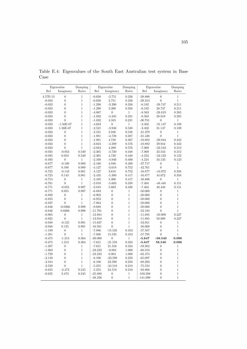
105
Table E.4: Eigenvalues of the South East Australian test system in BaseCase
Eigenvalue Damping Eigenvalue Damping Eigenvalue DampingRel Imaginary Ratio Rel Imaginary Ratio Rel Imaginary Ratio
4.57E-13 0 1 -0.638 -2.751 0.226 -28.886 0 1-0.033 0 1 -0.638 2.751 0.226 -29.313 0 1-0.033 0 1 -1.290 -3.390 0.356 -6.192 -28.747 0.211-0.033 0 1 -1.290 3.390 0.356 -6.192 28.747 0.211-0.033 0 1 -4.067 0 1 -8.563 -28.819 0.285-0.033 0 1 -1.032 -4.345 0.231 -8.563 28.819 0.285-0.033 0 1 -1.032 4.345 0.231 -30.781 0 1-0.033 -1.56E-07 1 -4.683 0 1 -3.402 -31.147 0.109-0.033 1.56E-07 1 -2.521 -3.946 0.538 -3.402 31.147 0.109-0.033 0 1 -2.521 3.946 0.538 -31.379 0 1-0.033 0 1 -1.981 -4.728 0.387 -31.438 0 1-0.033 0 1 -1.981 4.728 0.387 -10.882 -29.944 0.342-0.033 0 1 -3.024 -4.289 0.576 -10.882 29.944 0.342-0.033 0 1 -3.024 4.289 0.576 -7.069 -32.543 0.212-0.035 -0.053 0.549 -2.365 -4.720 0.448 -7.069 32.543 0.212-0.035 0.053 0.549 -2.365 4.720 0.448 -4.224 -34.133 0.123-0.493 0 1 -2.160 -4.946 0.400 -4.224 34.133 0.123-0.677 -0.100 0.989 -2.160 4.946 0.400 -37.717 0 1-0.677 0.100 0.989 -4.127 -3.618 0.752 -42.761 0 1-0.725 -0.143 0.981 -4.127 3.618 0.752 -16.877 -44.072 0.358-0.725 0.143 0.981 -2.435 -5.300 0.417 -16.877 44.072 0.358-0.754 0 1 -2.435 5.300 0.417 -48.896 0 1-0.761 0 1 -2.010 -5.603 0.338 -7.404 -48.448 0.151-0.771 -0.055 0.997 -2.010 5.603 0.338 -7.404 48.448 0.151-0.771 0.055 0.997 -6.883 0 1 -50.000 0 1-0.800 0 1 -6.903 0 1 -50.000 0 1-0.825 0 1 -6.953 0 1 -50.000 0 1-0.837 0 1 -7.864 0 1 -50.000 0 1-0.846 -0.0266 0.999 -9.688 0 1 -50.000 0 1-0.846 0.0266 0.999 -11.791 0 1 -52.194 0 1-0.905 0 1 -12.884 0 1 -11.885 -50.909 0.227-0.925 0 1 -13.910 0 1 -11.885 50.909 0.227-0.948 -0.125 0.991 -15.837 0 1 -53.951 0 1-0.948 0.125 0.991 -16.561 0 1 -56.069 0 1-1.189 0 1 -7.886 -15.535 0.453 -57.587 0 1-1.281 0 1 -7.886 15.535 0.453 -57.795 0 1-0.475 -1.213 0.364 -20.000 0 1 -5.647 -58.540 0.096-0.475 1.213 0.364 -7.651 -21.558 0.334 -5.647 58.540 0.096-1.387 0 1 -7.651 21.558 0.334 -59.302 0 1-1.663 0 1 -23.233 -0.004 1.000 -60.553 0 1-1.729 0 1 -23.233 0.004 1.000 -62.474 0 1-2.149 0 1 -6.100 -23.599 0.250 -65.097 0 1-2.344 0 1 -6.100 23.599 0.250 -68.293 0 1-2.539 0 1 -5.255 -24.518 0.210 -75.534 0 1-0.625 -2.473 0.245 -5.255 24.518 0.210 -92.866 0 1-0.625 2.473 0.245 -25.880 0 1 -103.288 0 1
-28.226 0 1 -141.098 0 1

106 APPENDIX E. IEEE SOUTH EAST AUSTRALIAN SYSTEM
Table E.5: Eigenvalues of the South East Australian system in Low-Inertiacase
Eigenvalue Damping Eigenvalue Damping Eigenvalue DampingRel Imaginary Ratio Rel Imaginary Ratio Rel Imaginary Ratio
5.12E-13 0 -1 -1.293 -2.966 0.400 -31.345 0 1-0.033 0 1 -1.293 2.966 0.400 -5.959 -30.809 0.190-0.033 0 1 -3.700 0 1 -5.959 30.809 0.190-0.033 0 1 -1.687 -3.884 0.398 -4.286 -33.750 0.126-0.033 0 1 -1.687 3.884 0.398 -4.286 33.750 0.126-0.033 0 1 -4.576 0 1 -34.515 0 1-0.033 0 1 -1.165 -4.646 0.243 -2.721 -36.133 0.075-0.033 -1.56E-07 1 -1.165 4.646 0.243 -2.721 36.133 0.075-0.033 1.56E-07 1 -3.028 -4.250 0.580 -37.796 0 1-0.033 0 1 -3.028 4.250 0.580 -1.265 -39.190 0.032-0.033 0 1 -2.393 -5.054 0.428 -1.265 39.190 0.032-0.033 0 1 -2.393 5.054 0.428 1.812 -39.368 -0.046-0.033 0 1 -3.477 -4.467 0.614 1.812 39.368 -0.046-0.033 0 1 -3.477 4.467 0.614 -8.347 -41.850 0.196-0.037 -0.056 0.554 -2.882 -4.900 0.507 -8.347 41.850 0.196-0.037 0.056 0.554 -2.882 4.900 0.507 -11.864 -41.653 0.274-0.493 0 1 -2.636 -5.330 0.443 -11.864 41.653 0.274-0.676 -0.100 0.989 -2.636 5.330 0.443 -10.765 -42.572 0.245-0.676 0.100 0.989 -4.697 -3.709 0.785 -10.765 42.572 0.245-0.724 -0.143 0.981 -4.697 3.709 0.785 -48.484 0 1-0.724 0.143 0.981 -2.950 -5.642 0.463 -50.000 0 1-0.754 0 1 -2.950 5.642 0.463 -50.000 0 1-0.762 0 1 -2.510 -6.107 0.380 -50.000 0 1-0.771 -0.056 0.997 -2.510 6.107 0.380 -50.000 0 1-0.771 0.056 0.997 -6.855 0 1 -50.000 0 1-0.801 0 1 -6.896 0 1 -52.313 0 1-0.827 0 1 -6.921 0 1 -56.124 0 1-0.838 0 1 -7.563 0 1 -58.495 0 1-0.850 -0.030 0.999 -8.576 0 1 -14.378 -57.587 0.242-0.850 0.030 0.999 -11.476 0 1 -14.378 57.587 0.242-0.904 0 1 -12.034 0 1 -60.061 0 1-0.927 0 1 -12.866 0 1 -61.470 0 1-0.947 -0.129 0.991 -15.389 0 1 -61.601 0 1-0.947 0.129 0.991 -15.722 0 1 -6.345 -62.552 0.101-1.271 0 1 -18.789 0 1 -6.345 62.552 0.101-1.360 -0.038 1.000 -20.000 0 1 -63.369 0 1-1.360 0.038 1.000 -22.639 0 1 -10.377 -64.836 0.158-0.724 -1.298 0.487 -12.170 -21.993 0.484 -10.377 64.836 0.158-0.724 1.298 0.487 -12.170 21.993 0.484 -66.093 0 1-1.655 0 1 -25.351 0 1 -71.711 0 1-1.691 0 1 -25.795 0 1 -73.283 0 1-2.229 0 1 -26.339 0 1 -4.147 -77.155 0.054-2.522 0 1 -28.519 0 1 -4.147 77.155 0.054-0.505 -2.758 0.180 -29.111 -0.081 1.000 -80.751 0 1-0.505 2.758 0.180 -29.111 0.081 1.000 -93.441 0 1-3.117 0 1 -7.778 -28.753 0.261 -103.459 0 1
-7.778 28.753 0.261 -144.905 0 1

Bibliography
[1] T. S. Borsche, T. Liu,and D. J. Hill. Effects of rotational inertia onpower system damping and frequency transients. To be presented at the54th IEEE Conference on Decision and Control, 2015.
[2] P. Kundur. Power System Stability and Control. McGraw-Hill Inc.,New York, 1994.
[3] G. Andersson. Lecture notes in Power System Analysis. EEH - PowerSystem Laboratory, ETH Zurich, September 2013.
[4] M. Gibbard, D. Vowles. Simplified 14-generator model of the south eastaustralian power system. IEEE Task Force on Benchmark Systems forStability Control, 2014.
[5] A. Ulbig, T. S. Borsche, and G. Andersson. Impact of low rotationalinertia on power system stability and operation. In Proceedings of the19th IFAC World Congress, pages 7290–7297, Cape Town, August 2014.B.Edward,Ed.
[6] W. Winter, K. Elkington, G. Bareux, and J. Kostevc. Pushing thelimits. IEEE Power and Energy Magazine, 13:60–74, January/February2015.
[7] T. S. Borsche, A. Ulbig, and G. Andersson. Impact of frequency controlreserve provision by storage systems on power system operation. InProceedings of the 19th IFAC World Congress, Cape Town, August2014.
[8] O. Megel, J.L. Matheu, and G. Andersson. Maximizing the potential ofenergy storage to provide fast frequency control. In 4th IEEE InnovativeSmart Grid Technologies Europe (ISGT 2013 Europe), Copenhagen,October 2013.
[9] EIRGRID, SEMO, SONI. System services review. TSO recommenda-tions. Report to the SEM Committee, 2012.
[10] Future ancillary services in ERCOT. ERCOT concept paper, 2013.
107
108 BIBLIOGRAPHY
[11] N. Miller, C. Loutan, M. Shao, and K. Clark. Emergency response.IEEE Power and Energy Magazine, 11:63–71, November/December2013.
[12] T. Ackermann, A. Ellis, J. Fortmann, et al. Code shift. IEEE Powerand Energy Magazine, 11:72–82, November/December 2013.
[13] IEEE/CIGRE Joint Task Force on Stability Terms and Definitions.Definition and classification of power system stability. Power Systems,IEEE Transactions on, 19:1387–1401, May 2004.
[14] M. Gibbard, P. Pourbeik, and D. Vowles. Small-signal stability, controland dynamic performance of power systems. Elsevier, 2014.
[15] D. Mondal, A. Chakrabarti, and A. Sengupta. Power System SmallSignal Stability and Control. Elsevier, 2014.
[16] IEEE Task Force on Load Representation for Dynamic Performance.Load representation for dynamic performance analysis. Power Systems,IEEE Transactions on, 8:472–482, May 1993.
[17] G. Andersson. Lecture notes in Power System Dynamics and Control.EEH - Power System Laboratory, ETH Zurich, February 2014.
[18] J. Lofberg. YALMIP: A toolbox for modeling and optimization in MAT-LAB. In Proceedings of the CACSD Conference, 2004.
[19] P. M. Anderson, A. A. Fouad. Power System Control and Stability.IEEE Press, 2003.
[20] B. Singh, Z. Hussain. Application of battery energy storage system(BESS) in voltage control and damping of power oscillations. In In-ternational Conference on Industrial and Information Systems (ICIIS).IEEE, August 2010.