University of South Florida University of South Florida

Scholar Commons Scholar Commons

Graduate Theses and Dissertations Graduate School

March 2021

Power System Optimization Methods: Convex Relaxation and Power System Optimization Methods: Convex Relaxation and

Benders Decomposition Benders Decomposition

Minyue Ma University of South Florida

Follow this and additional works at: https://scholarcommons.usf.edu/etd

Part of the Electrical and Computer Engineering Commons

Scholar Commons Citation Scholar Commons Citation Ma, Minyue, "Power System Optimization Methods: Convex Relaxation and Benders Decomposition" (2021). Graduate Theses and Dissertations. https://scholarcommons.usf.edu/etd/8818

This Dissertation is brought to you for free and open access by the Graduate School at Scholar Commons. It has been accepted for inclusion in Graduate Theses and Dissertations by an authorized administrator of Scholar Commons. For more information, please contact scholarcommons@usf.edu.

Power System Optimization Methods: Convex Relaxation and Benders Decomposition

by

Minyue Ma

A dissertation submitted in partial fulfillmentof the requirements for the degree of

Doctor of PhilosophyDepartment of Electrical Engineering

College of EngineeringUniversity of South Florida

Major Professor: Lingling Fan, Ph.D.Zhixin Miao, Ph.D.Nasir Ghani, Ph.D.

Tapas K. Das, Ph.D.Bo Zeng, Ph.D.

Date of Approval:Novmber 13, 2020

Keywords: alternating current optimal power flow, security constrained optimal power flow,relaxation exactness, model predict control

Copyright © 2021, Minyue Ma

Dedication

I dedicate this dissertation to my wife Danxu, I could not have done this without all of your love.

Acknowledgments

I would like to specially thank the following people, without whom I would not have achieved

this goal. To my committee chair, Dr. Lingling Fan, who has tirelessly supported my endeavors.

Thank you for always checking in on me, helping me out when I cannot find solutions, and teaching

me to be a qualified independent researcher. I deeply appreciate you nurturing the potential that

you saw in me. Dr. Zhixin Miao, thank you for inspiring and mentoring me. You have been my

professional role model, and it is you who opened my eyes to the amazing possibilities of research

in science. Dr. Zeng Bo, thank you for working with me to overcome difficult challenges. Your

comments and feedback were extremely helpful with my dissertation studies. Thank you to Dr.

Nasir Ghani, Dr. Tapas Das, and Dr. Yicheng Tu for their careful review of the dissertation and

constructive comments.

Thank you to my Ph.D. cohort at the University of South Florida Yin Li, Yangku Xu, Yi Zhou,

Miao Zhang, Li Bao, Zhengyu Wang, Ibrahim Alsaleh, and Abdullah Alassaf for inspiring me to

be a better student and bring joy in the Smart Grid Power Systems Laboratory.

Last but not least, I am grateful to my family members who have supported me throughout this

process. To my wife Danxu Ma, thank you for your love and steadfast support. I was not alone

because I always have you by my side. To my son Max, you are my little laughter. The day you

were born was the greatest moment of my life. I am highly in debt to my parents for supporting

me with their best wishes. To my father, “It’s like that with love, we may be close, we may be far,

but your love still surrounds me. . . wherever you are.”

Table of Contents

List of Tables iv

List of Figures v

Abstract vii

Chapter 1: Overview 11.1 General Introduction 11.2 Alternative Current Optimal Power Flow and Convex Relaxation 31.3 Exactness of Convex Relaxation 51.4 Model Predict Control for Power Electronic Application 51.5 Security Constrained Optimal Power Flow (SCOPF) Problem 61.6 Research Objectives 91.7 Outline of the Dissertation 9

Chapter 2: A Sparse Convex ACOPF Solver Based on 3-node Cycles 112.1 Introduction 112.2 ACOPF Problem 132.3 SOCP and SDP Relaxations of ACOPF 142.4 Prposed Sparse Convex Relaxation Formulation 16

2.4.1 Maximal Cliques Identification 172.4.2 Minimal Cycles in a Cycle Basis 172.4.3 Chordal Extension 182.4.4 Proposed Sparse Convex Relaxation Formulation 21

2.5 Case Study 222.5.1 Proposed Convex Relaxation 23

2.6 Conclusion 26

Chapter 3: Exactness of the Convex Relaxation 273.1 Introduction 273.2 Exactness Condition of SDP and SOCP Relaxation 293.3 Convex Iteration 29

3.3.1 Exactness Based on 3-node Cycles 293.3.2 Mathematical Proof of 3-node Cycles Based Exactness Condition 303.3.3 Principle of Convex Iteration 323.3.4 Sparse Implementation 33

3.4 Nonlinear Rank-1 Formulation 343.4.1 2× 2 Minor-based Rank-1 Constraints 34

i

3.4.1.1 The First Step: n-node Decomposition 363.4.1.2 The Second Step: Exactness Conditions Conversion 373.4.1.3 The Third Step: Constraints Reformulation 38

3.4.2 Rank-1 PSD Matrix-Based Nonlinear Programming Formulation 393.4.2.1 Cycle Basis Identification 393.4.2.2 Nonlinear Programming Problem Formulation 40

3.4.3 Voltage Recover Techniques 413.5 Case Studies 42

3.5.1 Rank-1 Solution Through Convex Iteration 423.5.2 Nonlinear Rank-1 Formulation 44

3.6 Conclusion 45

Chapter 4: Benders’ Decomposition for MPC of a Modular Multi-level Converter 474.1 Introduction 47

4.1.1 State-of-the-art MMC Switching Schemes 474.1.2 Our Contributions 48

4.2 Dynamic Model of MMC 504.3 Optimization Problem Formulation 524.4 Benders’ Decomposition Formulation 54

4.4.1 Subproblem 544.4.2 Cuts Introduced by the Subproblem 554.4.3 Master Problem 56

4.5 Case Study 564.6 Conclusion 60

Chapter 5: Security Constrained DC OPF Considering Generator Responses 625.1 Introduction 625.2 DC-PSCOPF Formulation 63

5.2.1 Equality Constraints: Power Flow Equations 645.2.2 Inequality Constraints: Component Limits 645.2.3 Generator Post-contingency Response Constraints 655.2.4 The MILP Formulation 66

5.3 The Proposed the Bilinear Formulation 675.3.1 Bilinear Formulation for Generator Response 675.3.2 Benders’ Decomposition: Approach 1 685.3.3 Benders’ Decomposition: Approach 2 69

5.3.3.1 McCormick Envelopes of the Bilinear Formulation 695.3.3.2 Benders’ Decomposition 72

5.4 Case Studies 745.4.1 Three-bus System 755.4.2 IEEE 118-bus System 775.4.3 Other Instances 79

5.5 Conclusion 80

ii

Chapter 6: Conclusion and Future Plan 816.1 Conclusion 81

6.1.1 A Sparse Convex ACOPF Solver Based on 3-node Cycles 816.1.2 Exactness of the Convex Relaxation 816.1.3 Benders’ Decomposition for MPC of a Modular Multi-level Converter 826.1.4 Security Constrained DC OPF Considering Generator Responses 82

6.2 Future Work 826.2.1 Security Constrained ACOPF 826.2.2 OPF in Renewable Energy Source Integrated Power System 82

References 84

Appendix A: Copyright Permissions 91

About the Author End Page

iii

List of Tables

Table 2.1 Size of the largest maximal cliques 17

Table 2.2 Results comparison 24

Table 2.3 Comparison with one strengthened SOCP solver 25

Table 2.4 SDPT3 results 25

Table 3.1 Convex iteration results 43

Table 3.2 Test case results 45

Table 3.3 Special test case results 45

Table 4.1 Parameters table 57

Table 4.2 Results comparison of Benders’ decomposition and SQP algorithm 58

Table 4.3 Binary solution 59

Table 5.1 Comparison Big-M MILP using Mosek and Approach 1. 69

Table 5.2 Conflict contingencies in all cases. 75

Table 5.3 3-bus system parameters. 75

Table 5.4 Comparison of objective values for the Big-M method and the proposed method. 77

Table 5.5 Solution for the N-1 contingency SCOPF 77

Table 5.6 118 bus contingency information. 78

Table 5.7 Comparison in different methods 80

iv

List of Figures

Figure 1.1 Power system structure. 1

Figure 1.2 Generator post-contingency response. 8

Figure 2.1 Chordal graph construction explanation. 18

Figure 2.2 Topologies of IEEE 14-bus case and IEEE 30-bus. 20

Figure 3.1 One chordless cycle become 3-node cycles with virtual lines. 36

Figure 3.2 Five-bus test case with two cycles. 40

Figure 3.3 Spanning tree of the five-bus test system. 40

Figure 3.4 Rank error converging for two instances. 44

Figure 4.1 Three phase MMC topology. 48

Figure 4.2 Three-level and Seven-level VSC PD-PWM scheme and switching status. 49

Figure 4.3 Single phase equivalent circuit of MMC. 50

Figure 4.4 An equivalent circuit of one phase of MMC. 51

Figure 4.5 Current tracking of Benders’ algorithm when T = 5 57

Figure 4.6 Convergence of the objective value for the master problem and sub-problemwhen T = 5. 58

Figure 4.7 Current tracking of Benders’ algorithm when T = 7. 58

Figure 4.8 Convergence of the objective value for the master problem and sub-problemwhen T = 7. 59

Figure 4.9 Current tracking of Benders’ algorithm when T = 10. 60

v

Figure 4.10 Convergence of the objective value for the master problem and sub-problemwhen T = 10. 60

Figure 5.1 Flow chart of Benders decomposition: Approach 1. 68

Figure 5.2 Flow chart of Benders decomposition: Approach 2. 70

Figure 5.3 3 bus system topology 76

Figure 5.4 Generators response for load variation. 76

Figure 5.5 Lower bound computed from the master problem converges while an maximumof the sub-problem solutions converges to zero. 78

Figure 5.6 Computation time against load level. 79

Figure 5.7 Computation time against contingency number. 79

vi

Abstract

Power system optimization methods are wildly used to solve power system problems. Engineers

adopt different methods to keep the reliability and efficiency of the power system operation, planning

and control. This dissertation focuses on the application and implementation of two optimization

methods: Convex relaxation and Benders’ decomposition.

The first part of the dissertation focuses on the application of convex relaxation to solve Alter-

nating Current Optimal Power Flow (ACOPF) problems. In the completed work, a 3-node cycle

based sparse convex relaxation is proposed to solve ACOPF problems. This method adds virtual

lines in minimal chordless cycles to decompose each of them into 3-node cycles. By enforcing the

submatrices related to 3-node cycles Positive Semi-Definite (PSD), the resulting convex relaxation

has a tight gap. For the majority of the test instances, the resulting gap is as tight as that of a

semi-definite programming (SDP) relaxation, yet the computing efficiency is much higher. Further-

more, to achieve the exactness of the convex relaxation, two algorithms are designed to decrease the

relaxation gap. The first method is based on the convex iteration technique. It could help the pro-

posed convex relaxation to achieve the exactness by enforcing all submatrices corresponding lines

and virtual lines rank-1. The second method is based on the nonlinear programming formulation

of ACOPF with the PSD matrix as the decision variable. In this method, the rank-1 PSD matrix

constraint is reformulated to equality constraints: all 2 × 2 minors of the PSD matrix are zeros.

The graph decomposition-based approach is implemented to reduce the computation burden.

In the second part of the work, the application of Benders’ decomposition is investigated through

two problems. The first problem is the Model Predict Control (MPC) problem for Modular Mul-

tilevel Converter (MMC). The objective of the MPC is to determine the best switching sequences

for the submodules in the MMC to track the phase current references for multiple time horizons.

vii

The MPC is formulated as a nonlinear mixed-integer programming (MIP) problem with the on/off

status of submodules as binary decision variables and MMC dynamic states such as phase currents,

circulating currents and submodule capacitor voltages as continuous decision variables. With a

large number of submodules and a large number of time horizons, the dimension of the nonlinear

MIP problem is difficult to handle. Our contribution is to formulate this problem and solve this

problem using Benders’ decomposition. In the second problem, an efficient Benders’ decomposi-

tion strategy is designed to solve the Security Constrained DCOPF (DC-SCOPF) with generator

response constraints. The major difficulties to solve such SCOPF are the large number of contingen-

cies and non-convexity of the generator response constraints. In this work, Benders’ decomposition

strategies were investigated to seek an efficient computing. We formulate the generator response

constraints via bilinear expressing, and adopt Benders’ decomposition to decompose the problem

into a master problem with multiple sub-problems, each associated with a contingency. Based

on the case study results, the proposed method has faster computing speed compares with the

traditional big-M based mixed-integer linear programming method.

This dissertation has led to three journal papers and one conference paper.

viii

Chapter 1: Overview

1.1 General Introduction

As an essential part of the running of model society, the power system which is the network to

generate, transmit, and use the electric power1.1, has been studied and developed over one hundred

years. Nowadays, the power system has been one of the largest engineering systems in the world.

It made hundreds of billions dollars revenue per year for electrical industry in united state. One of

the main challenges in power system operation is ensure the reliability and security of the system.

Meanwhile, the efficient power system operation is an important concern for the power system

engineers, because it can contributes to decrease the resource consumption, ensuring sustainability

with better planning, and increasing the economy benefits. To operate the power system reliably

and efficiently, optimization methods are wildly used to solve power system problems.

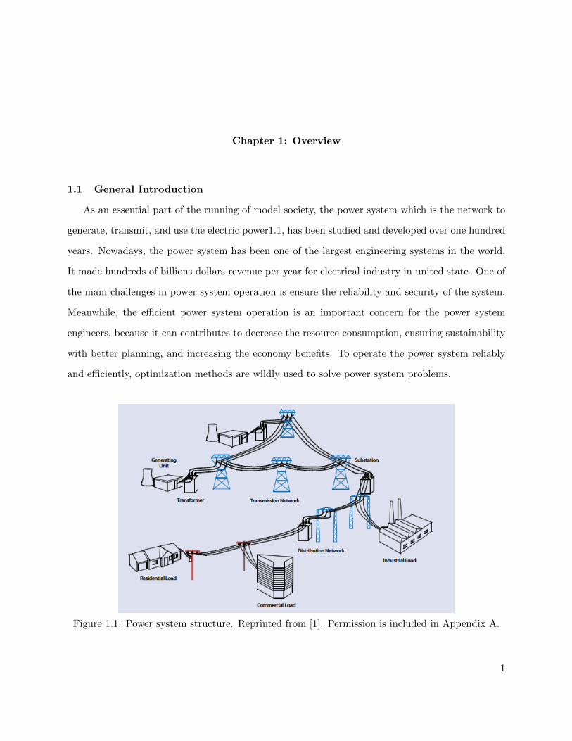
Figure 1.1: Power system structure. Reprinted from [1]. Permission is included in Appendix A.

1

Optimization methods have been used over the years for many power systems planning, oper-

ation, and control problems [2]. An power system optimization problem is a mathematical model

which is proposed to minimize or maximize a objective function, and satisfy some constraints based

on the physical requirements or decision making mechanism. In general, to solve real world power

system problems, the mathematical formulations of problems have to be derived based on some

assumptions, such as the Direct Current Optimal Power Flow (DCOPF) problem. However, even

under these assumptions to simplify problems, it is still not easy to obtain solutions for large size

problems. In general, real world power systems are large size, and complex because it includes

many different units and operation requirements. To solve the power system optimization prob-

lem accurately and efficiently, several optimization methods have been used to deal with different

formulations of problems, such as linear programming (LP), interior point (IP) method, quadratic

programming (QP), decomposition technical, mixed integer programming (MIP) and so on. There

are two methods attract a lot of interests in power system optimization researches. They are convex

relaxation and Benders’ decomposition.

In general, convex relaxation is implemented through relaxing some of the non-convex con-

straints and meanwhile extending the feasible region of the original problem, and the optimal value

of the relaxation problem is a lower bound of the optimal value of the original problem [3]. The

major application of convex relaxation is in Alternating Current Optimal Power Flow (ACOPF)

problems.

As the power flow equations are nonlinear, ACOPF problem is non-convex. Traditionally,

nonlinear programming methods have been applied to solve the problem [4]. The nonlinear pro-

gramming methods essentially find a local optimal solution in the feasible region that satisfies the

first-order optimality condition [5]. Examples presented in [5] indicate that local optima could

occur due to disconnected feasible region, loop flow, an excess of real or reactive power, or large

difference in voltage angles across lines. Thus, different initial point selections can result in different

solutions. As the convex relaxation is guarantee to converge and find the lower bound of original

problem, some new approaches to solve ACOPF can be developed based on it [6].

2

Benders’ decomposition is proposed by J.F.Benders [7] in 1962. The major objective of this

method is to simplify problems with complicating variables. Its fundamental idea is to separate

the problem into a master problem and a subproblem. In the subproblem, complicated variables

are considered as fixed value. Thus the subproblem could be solved easier. Iteratively, the dual

variables which are solved from the subproblem that will be used to generate Benders’ cuts and

add them to the master problem. And then, the solution of the complicated variables is returned

to the subproblem. This iteration process is repeated until the stop criteria is met.

When implementing Benders’ decomposition in power system problems, it is hard to directly

apply the classic Benders’ decomposition formulation which is presented in [7]. In general, we

need to choose the appropriate extended formulation of Benders’ decomposition to accurately and

effectively solve the problems [8]. Another important concern when using Benders’ decomposition

is how to formulate the problem models. Based on the research in [9], the problem formulation can

directly impact the performance of Benders’ decomposition.

This dissertation will cover topics about convex relaxation and Benders’ decomposition. For

convex relaxation, more efficient formulation for ACOPF problem is proposed, and algorithms to

improve the exactness for ACOPF convex relaxation is investigated. For Benders’ decomposition,

two problems are considered: model predict control problem for modular multi-level converter

and security constrained optimal power flow problem. In next sections, some backgrounds will be

provided for motivation of research.

1.2 Alternative Current Optimal Power Flow and Convex Relaxation

The first problem that will be discussed in this dissertation is the ACOPF problem. This

problem is first introduced by Carpentier in 1962 [10]. The objective function is to minimize

generation cost or power loss. The exact AC power flow equations are considered in the problem.

Full constraints are related to power grid physical characteristics, component limits, and network

operation limits. Depending on the practical requirements, some extra constraints may be included,

such as security constraints or stability constraints. As the power flow equations are nonlinear,

ACOPF is non-convex. Traditionally, nonlinear optimization solving methods, such as Newton-

type method [11] and interior point method [12], have been applied to solve the problem. These

3

methods essentially find a local optimal solution in the feasible region that satisfies the first-order

optimality condition. These local optima could occur because of disconnected feasible region, loop

flow, an excess of real or reactive power, or large difference in voltage angles across lines.

Conventionally, to avoid the major disadvantages which is brought by the nonlinear AC power

flow equations, the ACOPF will be simplified to directly current optimal power flow problem

(DCOPF). In DCOPF, the exact AC power flow constraints will be linearized to DC power flow

constraints. This simplification is based on three major assumptions: 1) all bus voltage magnitude

is 1 per unit; 2) all bus voltage angle is very small; 3) the transmission line resistor is ignorable.

DCOPF has better computational efficiency than ACOPF, but it ignored some important propriety

in the real power flow such as the reactive power transmission and might lead big error solutions

for stressed system.

In recent years, convex relaxation has attracted a lot attentions on solving ACOPF problem,

because it is capable to find provable lower bound of the solution to the original ACOPF problem.

The two major relaxation techniques are semi-definite programming (SDP) relaxation and second-

order cone programming (SOCP) relaxation. SDP relaxation was first applied to solve ACOPF in

Bai et al [13]. SOCP was proposed in Jabr for radial networks [14]. SDP relaxation of ACOPF has

shown to be a very strong convex relaxation to be original non-linear formulation. Nevertheless,

the disadvantage of SDP is its expensive computational cost. Comparing with the SDP relaxation,

SOCP has better computational efficiency. But its relaxation gap tend to be higher, especially for

the mesh network.

Find a faster and more accurate method to solve ACOPF problem is important, because it could

efficiently reduce the cost in power system. Based on the study in [15], even a 5% computation

efficiency improvement could lead billions dollars saving in each year. Thus, the first part of this

dissertation will focus on increasing the computation efficiency of the convex relaxation method,

and develop the computational strategy to decreasing the relaxation gap, so that leads to high

quality, near global optimal solutions.

4

1.3 Exactness of Convex Relaxation

Though it has been studied that SDP relaxation can give global optimum for many IEEE test

systems while the solutions are feasible to the original ACOPF problems (termed as “SDP exact”)

in [16], in some other cases, SDP relaxation leads to solutions not feasible or SDP inexact [5,17,18].

Thus, research efforts have been devoted to achieve SDP exactness, e.g., [19, 20].

The exactness conditions for SDP and SOCP relaxations are presented in [6]. Research has been

conducted to achieve exactness for convex relaxation through exploiting the exactness conditions.

In [19,20], objective functions are modified to include penalty related to the rank-1 constraint. [21]

treats an ACOPF problem as an SDP relaxation problem and a non-convex rank-1 feasible region

mapping problem. Alternating direction method of multipliers (ADMM) iterative procedure is then

applied. In [22], the exactness constraint is reformulated as minor constraints and approximated

by convex constraints. A strengthened SOCP relaxation of ACOPF is then solved. [23] proposes

an convex iteration algorithm to solve a convex problem with a regularization term related to

the maximal eigenvalue of the full PSD matrix. With the regularization term achieving zero, the

solution achieves global minimum. In [24], the non-convex OPF branch flow equation is decomposed

into SOCP constraint and a non-convex constraint related to the difference of two convex functions.

The concave term is then approximated by linear functions and updated in each iteration. A

sequential convex optimization method is implemented to carry out the iteration.

The approaches above lead to exact solutions in many cases. However, large gaps are still

observed for special cases [20].

1.4 Model Predict Control for Power Electronic Application

As an advanced control method, MPC is very successful on its application for the control of

power converters [25]. Its basic principle is to generate a system dynamic model based minimizing

optimization problem, and provide the solutions to the controller for driving the system to reach

the control target (Generally will be formulated as the objective function in the MPC optimization

problem). For MPC for power electronics, the switching signals are normally chosen as the decision

variables of the optimization problem. Conventionally, the gate signals are normally generated by

pulse width modulation (PWM). The PWM gate signal generator compares the reference signal

5

with a high frequency carrier waveform. The frequency of the resulting switching signal will be close

to the carrier waveform, which is not necessary at all the time. Furthermore, in real applications,

the power electronics gates are not ideal gate that has zero resistance for turning-on mode, infinite

resistance for turning-off mode, and zero reacting time for switching the gate status. So the higher

switching frequency will results higher switching loss, and the power loss is normally turned into

heat generation, which is unwanted for most of the applications.

The concept of MPC is to predict the switching actions for the next N horizons and apply the

switching action of the current step to the switch gates. With time evolving, the microprocessor

calibrates the actions for the future horizons and sends the control signals related to the current

time step to the switch gates. Therefore the MPC for power electronics should be able to provide

a switching signal with a variable switching frequency. The gates should only switch its status

when necessary. Another difference between MPC and PWM is the input of the modulator. For

conventional PWM method, the input of the modulator is the voltage reference. The current

tracking is achieved by a feedback control loop with vector control. While the MPC control works

as a current regulator in particular. With MPC, the switching signal for the power electronics

is directly generated by the MPC controller with current reference and measurement from the

system [26] [27]. The major difficulty to solve the MPC for power electronic devices is that the

system dynamic model of power electronic devices could be nonlinear with binary terms, such as

the Modular Multi-level Converter (MMC). The dynamic model of the MMC includes a lot integer

variables for each module’s switch status, and bilinear terms about the output current. It means

the MPC problem of MMC is a nonlinear MIP problem which generally hard to obtain the solution

and high computing burden. Thus, it is worth to design a more efficient method to solve the MPC

problem.

1.5 Security Constrained Optimal Power Flow (SCOPF) Problem

Security constrained OPF (SCOPF) is an extension of OPF. Its purpose is to find an operation

point to optimize an objective function at base case, while satisfying all pre-contingency (base

case) and post-contingency constraints. There are two major approaches to formulate the SCOPF

problem, which are preventive approach and corrective approach. In the preventive approach,

6

any undesirable operation conditions will be prevented from the beginning if the contingency hap-

pens. Thus, the re-dispatches are not allowed for the control variables, except those automatically

response to contingencies, such as the primary and secondary frequency response [28]. In the cor-

rective approach, the constraints violations which are caused by the contingency can be removed

within a certain time limits by the predefined corrective actions, such as switching the transmission

lines or generators [29]. It means the SCOPF with corrective approach is easier to get more opti-

mal solution, but has to consider more variables and constraints which will make the system more

difficult to be solved. This dissertation focuses on the preventive-SCOPF (PSCOPF), because in

the industrial application, preventive-SCOPF (PSCOPF) is dominated [30].

The major challenge to solve PSCOPF is the large size of the problem. Even we only consider

the ”N-1” criterion, the computation cost of the SCOPF with all contingencies considered could be

too high. To address this issue, the decomposition technique is implemented to reduce the decom-

position cost. There are two major techniques are implemented in the SCOPF problem, Benders’

decomposition and alternating directions methods of multiplier [31]. In Benders’ decomposition,

the SCOPF problem is decomposed into one master problem and multiple subproblems, each as-

sociated to a contingency. The problem will be solved based on the iteration, and feasibility cuts

generated by subproblems will be added to the master problem in each iteration. The problem

will be considered as solved until the there is no feasibility cut need to be added. In ADMM, the

SCOPF will be decomposed into a number of smaller subproblems related to each contingency. All

subproblems can be solved parallel. ADMM also need to be solved based on the iteration. But

different with Benders’ decomposition, the feasible regions of subproblems have not been changed

during iterations.

Another issue in PSCOPF is about how to formulate the online generator responses for the

generator outage contingencies. A generator’s post-contingency response is illustrated in Fig 1.2,

where Pmaxgi and Pmin

gi are the upper and lower limits of the ith generator’s active power output

respectively; P(0)gi is the power in pre-contingency state; P

(k)gi is the power in post-contingency state;

∆(k) is the active power imbalance in the system right after the contingency before AGC; α(k)i is

the participation factor corresponding to the slope. For each generator, the participation factor is

7

the ratio of the output power response of this generator in the total power deviation. Three feasible

regions are denoted in the Fig. 1.2.

Δ Pgi(k)

Pgimax-Pgi

(0)

(1)

(2)

(3)

Δ(k)

Pgimin-Pgi

(0)

Ɵ

ɑ=tan (Ɵ)

Figure 1.2: Generator post-contingency response.

Considering the generator response is PSCOPF is mathematically challenging because the re-

sponse has to be modeled as an nonlinear, non-convex constraints. In conventional formulation,

the generator outages are ignored in the PSCOPF [32] [33] [34], or the power output of generators

are considered as freezing when the generator outage contingencies happen. However, in practical

situations, generator outage is common and the remaining online generators will try to compensate

the power loss instantaneously because it is governed by the automatic generator control (AGC)

setting.

Modeling the non-convex generator response characteristics has been carried out in the litera-

ture. In [35] and [36], the authors assume that the generator responses in post-contingency always

follow their predefined participation factors, i.e. only region (2) is considered. This formulation

could simplify the problem as the generator responses are defined by a set of linear constraints.

However, due to the inaccurate representation of the feasible region, the solutions are not correct.

Alternatively, mixed integer linear programming (MILP) formulation has been designed in [37]

and [38]. The generator response constraint is formulated as a set of MILP constraints based on

big-M technique. The major disadvantage of this method is the well-known disadvantage related

to big-M formulation , i.e., the difficulty of finding a suitable value M .

8

1.6 Research Objectives

The major research purpose of this dissertation is to study the application for power system

optimization methods. In particular, the dissertation objectives include four major parts:

• Find a more efficient convex relaxation methods to solve the alternative current optimal power

flow problem

• Investigate new algorithms to improve the exactness of the convex relaxation formation for

the ACOPF problem.

• Build the MPC problem model for MMC, and implement Benders’ decomposition method to

solve the problem.

• Develop a new method to solve security constrained optimal power flow problem while con-

sidering the generator response constraints.

The first two objectives plan to enhance the performance of convex relaxation and improve its

exactness, objective 3 and 4 aim to build appropriate problem models for Benders’ decomposition

and improve the computation efficiency for the problems.

1.7 Outline of the Dissertation

The dissertation is organized as follow:

• Chapter 1 Introduces the importance of power system optimization methods, and presents a

brief literature reviews for the problems tackled in this dissertation.

• The proposed convex relaxation method to solve ACOPF will be presented in the Chapter

2. This chapter first introduces the classic formulation of the ACOPF, and the SOCP and

SDP relaxation formulation of ACOPF problem in section 2.2 and 2.3 respectively. In section

2.4 presents the maximal clique- and cycle-based convex relaxation formulations. Finally,

numerical results are presented in section 2.5.

• Chapter 3 investigate two methods to improve the exactness of convex relaxations. The first

method is based on the convex iteration. The second method is based on the Rank-1 PSD

9

Matrix-Based Nonlinear Programming. Section 3.3 presents the principle of the convex itera-

tion and its implementation on the convex relaxed ACOPF problem. The formulation of the

ACOPF which is based on rank-1 PSD Matrix-Based Nonlinear Programming is introduced

in section 3.4. The performance of these two methods on improving the exactness of the

convex relaxation is discussed in the section 3.5.

• Chapter 4 introduce the Benders’ decomposition based MPC for MMC. In section 4.2, the

dynamic model for MMC is derived. Section 4.3 gives the details about the formulation

of the MPC as a nonlinear MIP problem. Section 4.4 gives the Benders’ decomposition

algorithm. The comparison of the performance for nonlinear MIP and Benders’ decomposition

is compared through case study in the section 4.5.

• Chapter 5 presents the proposed method to solve SCOPF with generator response constraints.

In section 5.2, we introduce SCOPF and the MILP formulation of the generator response

constraints. The proposed bilinear formulation and tow Benders’ decomposition strategies

are described in section 5.3. And case study is presented in the section 5.4.

• Chapter 6 concludes the dissertation and proposes future works by extending the research to

more complex and practical power system. And the further study to implement distributed

computation algorithm to solve SCOPF problem.

10

Chapter 2: A Sparse Convex ACOPF Solver Based on 3-node Cycles

2.1 Introduction

1Alternating current optimal power flow (ACOPF) is a classic optimization problem in power

systems [40]. The objective is to minimize generation cost or power loss. Constraints are related to

power grid physical characteristics (e.g., power flow equations), component limits (e.g., generator

capacity limits, transmission line limits) as well as network operation limits (e.g., voltage limits).

Depending on the practical requirements, some extra constraints may be included, such as security

constraint [29], or stability constraint [41,42].

As the power flow equations are nonlinear, ACOPF is non-convex. Traditionally, nonlinear

optimization solving methods, e.g., Newton’s method and interior point method , have been applied

to solve the problem [4]. These methods essentially find a local optimal solution in the feasible

region that satisfies the first-order optimality condition [5]. Examples presented in [5] indicate that

local optima could occur due to disconnected feasible regions, loop flow, an excess of real or reactive

power, or large difference in voltage angles across lines.

Global optimum means guaranteed least cost. In recent years, applying convex relaxation

techniques to solve ACOPF problem and find global minimum has been carried out and a tutorial

can be found in [6, 43]. Relaxation problems find the lower bound of the solution to ACOPF. The

two major relaxation techniques are SDP relaxation, and SOCP relaxation. SDP relaxation was

first applied to solve ACOPF in [13]. SOCP relaxation was proposed in [14] for radial networks.

In radial networks, SOCP relaxation and SDP relaxation are equivalent [6].

SDP relaxation of ACOPF has shown to be a very strong convex relaxation to the original

non-convex formulation [16, 44]. Nevertheless, the disadvantage of SDP relaxation is its expensive

computational cost.

1This chapter was published in Electric Power Systems Research [39]. Permission is included in the Appendix A.

11

For that reason, sparse technique has been exploited for SDP relaxation [19, 45, 46]. The main

theorem is the PSD matrix completion theorem [47], which states that if every submatrix related

to every maximal clique in a chordal graph is PSD, then the partial symmetric matrix Xch corre-

sponding to the chordal graph can be completed as a full PSD matrix X 0. The graph related to

the topology of a power grid is usually not a chordal graph. To obtain a chordal graph, Cholesky

factorization has been used to find chordal extension [45]. Detailed implementation procedure of

Cholesky factorization and sparse SDP relaxation can be found in [46]. Instead of finding maximal

cliques and further a clique tree through Cholesky factorization, tree width decomposition can also

be used to find a clique tree [19]. This method has been implemented in a software package for

SDP relaxation of OPF [48].

The aforementioned researches focus on sparse SDP relaxation. On the other hand, there is

a category of research focusing on strengthening SOCP relaxation [49, 50]. Compared to SDP

relaxation, SOCP relaxation is computationally more efficient. Nevertheless, the feasible region

of SOCP relaxation is less tight. Strengthening SOCP relaxation has been studied in [49, 50] by

implementing cutting plane algorithms, i.e., iteratively adding valid inequalities, including SDP

based ones. The principle of the methods in [49,50] is based on the fact that for a PSD matrix, its

submatrices corresponding to cycles in a cycle basis are PSD. If a submatrix of the solution of the

SOCP is not PSD, a valid inequality can be constructed to reduce the search region. The constraint

can be constructed using duality concept in [49] and shortest Euclidean distance technique in [50].

In this research, we explore an alternative computationally friendly method that can strengthen

SOCP relaxation. Instead of iteratively solving and strengthening the SOCP relaxation by cutting

plane algorithms, we propose to directly add maximal clique-based and cycle-based SDP feasibility

constraints in the SOCP relaxation. Those added constraints enforce the submatrices related to

maximal cliques and cycles to be PSD.

Further, we conduct chordal relaxation for chordless cycles. A chordless cycle of size n can be

decomposed into 3-node cycles or cliques by adding (n− 3) virtual edges. Adding virtual lines has

also been adopted by other researchers. For example, [51] proposed to add virtual lines between

12

the reference bus and all its non-adjacent buses. By enforcing all submatrices related to the virtual

lines PSD, the resulting convex relaxation in [51] is stronger than the original SOCP.

Compared to [51], our method of virtual line addition based on chrodless cycle 3-node decom-

position results in less virtual lines and thus is more efficient. Overall, this method results in a

stronger convex relaxation compare to SOCP relaxation. All 2 × 2 principal submatrices of the

full matrix are guaranteed to be PSD. Further, all maximal cliques with size greater than 2 in

the original power grid graph, and the 3-node cycles constructed from chordless cycles are PSD.

The computing efficiency has been compared with sparse SDP methods [46] [19] and is found to

be higher. Though the graph after chordal extension is not guaranteed to be a chordal graph, the

resulting formulations in many cases are as strong as SDP relaxation.

The major contributions in this chapter is twofold. First, we answer a question naturally arise

from the research results from [49] and [50]: Will a PSD solution be found if its SOCP solution’s

submatrices related to cycles in a cycle basis are PSD? We demonstrate that chordal relaxation

for every cycle in a cycle basis cannot result in a chordal graph. Hence, there is no guarantee that

the strengthened SOCP in [49] and [50] can lead to SDP solution eventually. Second, we propose

a stronger convex relaxation compared to SOCP by enforcing minimal cycles of a cycle basis PSD.

This enforcement can be further replaced by 3-node cycle PSD enforcement. The proposed solver is

implemented in CVX platform and shows higher computing efficiency compared with sparse SDP

methods [46] [19].

2.2 ACOPF Problem

First we describe the original formulation of ACOPF. Considering a power network, we denote

the buses as i ∈ B, the transmission line as (i, j) ∈ L and the generators as i ∈ G. The admittance

matrix is defined as Y where Y = G+jB, G and B are the conductance matrix and the susceptance

13

matrix, respectively. The classic ACOPF problem is formulated as follows.

minV,θ,Pg ,Qg

∑k∈G

C2kP2gk + C1kPgk + C0k (2.1a)

P gi − Pdi =

n∑j∈Adji

ViVj(Gij cos θij +Bij sin θij), i ∈ N (2.1b)

Qgi −Qdi =

∑j∈Adji

ViVj(Gij sin θij −Bij cos θij), i ∈ N (2.1c)

|Sij(V, θ)|≤ Smaxij , (i, j) ∈ L (2.1d)

Pmingi ≤ Pgi ≤ Pmax

gi , i ∈ G (2.1e)

Qmingi ≤ Qgi ≤ Qmax

gi , i ∈ G (2.1f)

V mini ≤ Vi ≤ V max

i , i ∈ N (2.1g)

where C2k, C1k and C0k are the coefficients of the quadratic cost function for the generator k, P gi ,

Qgi are the total generated active and reactive powers from the generators connected at Bus i, P di ,

Qdi are total demanded active and reactive powers at Bus i, Adji is the set of the buses that have

direct connection with Bus i, V ∈ R|N | and θ ∈ R|N | are the voltage magnitude vector and angle

vector, respectively, Sij is the complex power flow on the transmission line from Bus i to Bus j. |.|

notates the cardinality of a set. The decision variables are Pg, Qg, V, θ .

2.3 SOCP and SDP Relaxations of ACOPF

The ACOPF formulation is a non-convex optimization problem. This can be shown by the

power injection equality constraints(2.1b) and (2.1c). Note that the equality constraints of power

injections are nonlinear in terms of V and θ. This yields the ACOPF problem non-convex. Relax-

ations have been developed in the literature to have a convex feasible region. These methods deal

with new sets of decision variables to replace V and θ.

14

In SOCP relaxation [14], a new set of variables cij and sij is used to replace the voltage phasors

Vi 6 θi, i ∈ B.

cii = V 2i , i ∈ B

cij = ViVj cos(θi − θj), (i, j) ∈ L

sij = −ViVj sin(θi − θj), (i, j) ∈ L

where cij = cji and sij = −sji.

It is easy to find the following relationship:

c2ij + s2ij = V 2i V

2j = ciicjj . (2.2)

There will be |L| number cij and sij . If there is no direct connection between Bus i and Bus

j, the power injection equations will not contain cij nor sij . The decision variables V and θ are

replaced by cii, i ∈ B, and cij , sij , (i, j) ∈ L. The dimension of the new set of the variables is

2|G|+|B|+2|L|.

With the new set of variables, power injection equations (2.1b) and (2.1c) are now linear. The

line flow limit constraints become second-order cone constraints. The only constraint that makes

the program non-convex is (2.2). This constraint can be relaxed as a second-order cone:

c2ij + s2ij ≤ ciicjj , (i, j) ∈ L (2.3)

This relaxation was first proposed in [14] for ACOPF and named as SOCP relaxation.

In SDP relaxation proposed by [13], the decision variables related to voltage phasors are replaced

by a matrix X = V VH

, where Xij = V iV∗j = cij− jsij , superscript H denotes Hermitian transpose

for a vector and superscript ∗ means complex conjugate for a scalar.

15

(2.3) can be rewritten as

∣∣∣∣∣∣∣Xii Xij

Xji Xjj

∣∣∣∣∣∣∣ = XiiXjj −XijXji ≥ 0. (2.4)

Based on the definition X = V VH

, it is obvious that X is PSD and rank-1.

X = XH , X 0, and rank(X) = 1 (2.5)

where X 0 means that this matrix is PSD.

The power injection constraints are linear with the elements of X. With the rank-1 constraint

relaxed, the problem is a convex problem: SDP relaxation of ACOPF. For tree networks, SOCP

relaxation and SDP relaxation are equivalent [44]. For meshed network, the SOCP constraint (2.3)

or (2.4) enforces only 2×2 principal submatrices related to lines PSD. For cliques with sizes greater

than 2 and cycles, SOCP relaxation does not guarantee the related submatrices PSD.

2.4 Prposed Sparse Convex Relaxation Formulation

Instead of dealing with a full matrix X for the entire grid, for each maximal clique and each cycle

in the cycle basis of the network, we impose the PSD constraint for the corresponding submatrix

X(i). This is equivalent to first conduct chordal extension to make a chordless cycle of size n a

clique and then enforce the related n × n submatrix PSD. On the other hand, there is a more

efficient way of chordal extension for a chordless cycle: A cycle can be decomposed into 3-node

cycles. This approach can save computing cost due to the reduction of the size of the PSD matrices

(all 3× 3). We further examine if such chordal relaxation can lead to a chordal graph for the entire

power grid. If so, we have a sparse SDP relaxation. If not, we have a stronger convex relaxation

compared to SOCP.

In this section, we first review a few graph theory techniques that will be used to identify

maximal cliques and chordless cycles. We then examine the proposed chordal extension for various

examples and check if they can lead to a chordal graph. Finally, we give the proposed sparse convex

relaxation formulation.

16

2.4.1 Maximal Cliques Identification

Given a graph’s boolean adjacency matrix, all maximal cliques can be identified using Bron-

Kerbosch algorithm [52]. In this project, a MATLAB toolbox [53] based on Bron-Kerbosch algo-

rithm has been used to identify maximal cliques. Table 2.1 presents the size of the largest maximal

cliques in test instances. We may observe that all grids have largest maximal cliques with size 3 or

less, except IEEE 118-bus system. This system has a maximal clique of size 4.

After identifying the maximal cliques in a power grid, the next step is to identify chordless

cycles.

Table 2.1: Size of the largest maximal cliques

Test case size Test case size

nesta case3 lmbd 3 nesta case4 gs 2nesta case5 pjm 3 nesta case14 ieee 3nesta case30 ieee 3 nesta case57 ieee 3nesta case118 ieee 4 nesta case300 ieee 3nesta case1354 pegase 3 nesta case2383wp 3nesta case2736sp mp 3 nesta case2737sop mp 3nesta case2746wop mp 3 nesta case2746wp mp 3nesta case3012wp mp 3 nesta case3120sp mp 3

2.4.2 Minimal Cycles in a Cycle Basis

Cycle basis identification algorithm in [54] is used to identify the cycle basis. A related MATLAB

toolbox is also available [55]. The procedure of cycle basis identification is to first build a spanning

tree. The edges that are not in the spanning tree are identified as the back edges. The number

of back edges is the number of the cycles in a cycle basis. The back edges are added back to the

spanning tree one by one. If a back edge is added, one cycle is identified. The resulting cycles are

not necessarily minimal cycles. In this project, we aim to find minimal cycles. The justification of

minimal cycles is given by the following example.

Fig. 2.1 presents an example graph to illustrate the chordal graph construction and why minimal

chordless cycles are desired. Fig. 2.1(a) presents the original topology of a graph. The definition

of a chordal graph is that all cycles of four or more vertices have a chord. This original graph is

not a chordal graph since there is no chord for cycle 2, 3, 4, 5.

17

1

25

34

1

25

34

1

25

34

(a)

(b) (d)

1

25

34

(c)

Figure 2.1: Chordal graph construction explanation.

As cycle basis identification algorithm does not guarantee minimal chordless cycles, we may

end up with two cycles identified for Fig. 2.1(a): 1, 2, 5 and 1, 2, 3, 4, 5. Suppose that for the

second cycle identified, two lines: 1 − 4 and 1 − 5 are added. The resulting graph shown in Fig.

2.1(b) is not a chordal graph since there is no chord in cycle 2, 3, 4, 5.

On the other hand, if we are able to identify the two minimal chordless cycles as 1, 2, 5 and

2, 3, 4, 5, we may add a chord in the 4-node cycle (line 2− 4 or line 3− 5). The resulting graphs

shown in Fig. 2.1(c)(d) are two chordal graphs.

To find minimal chordless cycle in a cycle basis, we use shortest path algorithm. For every back

edge, first, the entire graph will have this back edge removed. The two nodes of the back edge are

defined as the start node and the destination node. Shortest path in the modified graph from the

start node to the destination node can be found using MATLAB 2017’s graph toolbox.

2.4.3 Chordal Extension

A further graph decomposition strategy is employed to have virtual lines added and have any

minimal chordless cycles with size greater than 3 to be decomposed into cycles with 3 nodes. The

number of virtual lines added is (n− 3) where n is the size.

18

The graph after chordal extension is not necessarily a chordal graph. Though these cycles can

be extended into chordal graphs, the entire grid may still have other cycles with size greater than

3. If a graph is chordal, then there exists a permutation to make the Cholesky factorization with

zero filling. On the other hand, if there exists Cholesky factorization with non-zero filling, then the

graph is not a chordal graph. In this project, we adopt MATPOWER’s SDP toolbox [56] function

”maxcardsearch” written by Dan Molzahn to conduct the check.

IEEE 14-bus system and IEEE 30-bus system are used as two examples in Fig. 2.2 to demon-

strate minimal cycles and 3-node decomposition by adding virtual lines (dotted lines). If the

resulting graph after 3-node decomposition is not a chordal graph, Cholesky factorization is then

conducted. The additional virtual lines will be added as solid magenta lines. We can see that the

14-bus system after 3-node decomposition is a chordal graph while the 30-bus system after 3-node

decomposition is not a chordal graph. Additional lines should be added to achieve a chordal graph.

Two cycles with size greater than 4 are identified for the 14-bus system. They are 4, 5, 6, 13, 14,

9 and 4, 5, 6, 11, 10, 9. Node 6 is used as the starting node to add virtual lines for both cycles.

Total there are 4 virtual lines added to decompose the two cycles into 3-node cycles. The resulting

graph is a chordal graph.

Four cycles with size greater than 4 are identified for the 30-bus system. They are 16, 12, 4, 6, 10,

17, 25, 27, 28, 6, 10, 22, 24, 18, 15, 12, 4, 6, 10, 20, 19, and 23, 15, 12, 4, 6, 10, 22, 24. For the

first cycle, 3 virtual lines are added starting from node 16: 16 − 4, 16 − 6, and 16 − 10. Simi-

larly, virtual lines are also added. The resulting graph, however, is not a choral graph. Cholesky

factorization is then conducted and 5 virtual lines are found: 25 − 23, 6 − 12, 16 − 23, 16 − 18,

23− 18.

We have also conducted chordal extension to make every minimal cycle a clique. The resulting

graphs for systems with size more than 57 are found as not chordal graphs.

This study answers a question naturally arise from the research on cycle-based SDP feasibility

enforcement presented in [49] and [50]: Will a PSD solution be found if its SOCP solution’s sub-

matrices related to cycles in a cycle basis are PSD? We demonstrate that chordal relaxation for

19

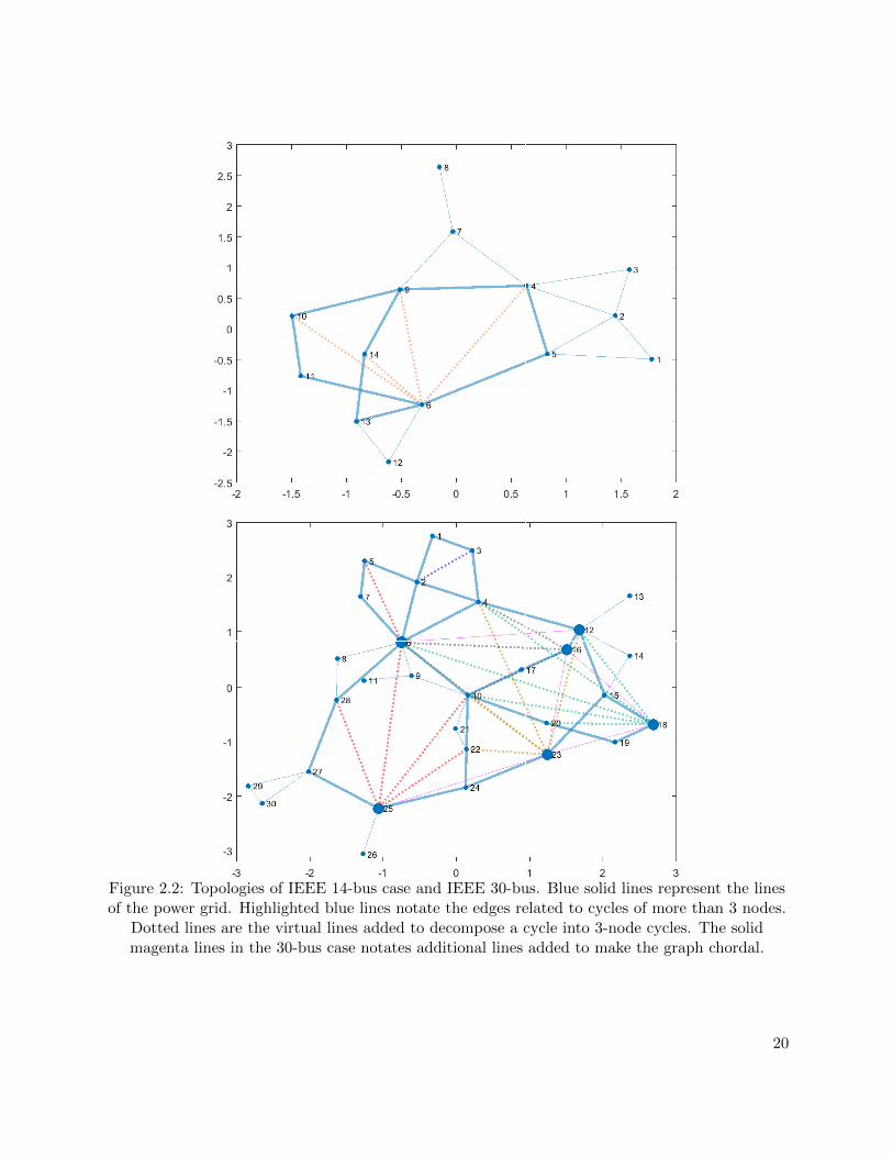
Figure 2.2: Topologies of IEEE 14-bus case and IEEE 30-bus. Blue solid lines represent the linesof the power grid. Highlighted blue lines notate the edges related to cycles of more than 3 nodes.

Dotted lines are the virtual lines added to decompose a cycle into 3-node cycles. The solidmagenta lines in the 30-bus case notates additional lines added to make the graph chordal.

20

each cycle of a cycle basis cannot result in a chordal graph. Hence, there is no guarantee that the

strengthened SOCP in [49] and [50] can lead to SDP solution eventually.

2.4.4 Proposed Sparse Convex Relaxation Formulation

With no guarantee of a chordal graph, the 3-node decomposition leads to a sparse convex

relaxation. The decision variables of the proposed convex relaxation include cii (i ∈ B) and cij , sij

((i, j) ∈ L ∪ V). V notates that the set of virtual lines for 3-node cycles decomposition. Note

that compared to SOCP formulation whose decision variables include cij and sij for every line, the

proposed convex relaxation has additional decision variables related to virtual lines.

Sparse matrix technique is employed in the proposed convex relaxation formulation. A sparse

matrix X is defined to have its diagonal elements and elements related to lines and virtual lines

non zero. The rest elements are all zeros.

Xii = cii, i ∈ B (2.6a)

Xij = cij − jsij , (i, j) ∈ L ∪ V (2.6b)

Xji = cij + jsij , (i, j) ∈ L ∪ V (2.6c)

The sparse convex relaxation enforces all submatrices related to maximal cliques PSD. The maximal

cliques include the maximal cliques with size greater than 2 from the original graph, 3-node cycles

resulting from decomposition, and rest lines. The formulation is presented in (2.7).

In the formulation (2.7), SMC notates the set of maximal cliques and Xi notates the submatrix

of X related to ith maximal clique. gij = real(yij) and bij = imag(yij) and yij is a branch (between

Bus i and Bus j)’s admittance. (2.7b) and (2.7c) represent the net power injection constraints at

each bus. (2.7f) is the line flow limit constraint. (2.7g) is the voltage limit constraint. (2.7h) are the

generator power limit constraints. (2.7i) enforces PSD for submatrices related to maximal cliques.

Formulation (2.7) is a general SOCP/SDP ACOPF solver employing sparse matrix technique.

If chordal extension of a power grid can result in a chordal graph, the above solver is a SDP solver.

On the other hand, if the graph is not a chordal graph, the above solver is a stronger convex

21

relaxation solver than SOCP. For comparison, we have employed Cholesky factorization method to

find a chordal graph (Solver B in section 2.5).

min f(Pg) (2.7a)

s.t. P gi − Pdi =

∑j∈δi

(Gijcij −Bijsij), i ∈ B (2.7b)

Qgi −Qdi =

∑j∈δi

(−Gijsij −Bijcij), i ∈ B (2.7c)

Pij = gij(cii − cij)− bijsij , (i, j) ∈ L (2.7d)

Qij = −bij(cii − cij)− gijsij , (i, j) ∈ L (2.7e)√P 2ij +Q2

ij − Smax ≤ 0, (i, j) ∈ L (2.7f)

(V mini )2 ≤ cii ≤ (V max

i )2, i ∈ B (2.7g)

Pming ≤ Pg ≤ Pmax

g , Qming ≤ Qg ≤ Qmax

g (2.7h)

Constraints (2.6)

For all cliques MC,

X(i) 0, i ∈ SMC (2.7i)

2.5 Case Study

Instances from the NICTA test archive [57] are tested using the proposed formulation. Ad-

ditional instances with large gaps (case9mod, case39mod1, case300mod) are from [5]. We also

implemented the method in [45] and [46] and developed a sparse SDP solver based on a chordal

graph using Cholesky factorization. Cholesky factorization of a Hermitian semi-definite matrix A

is defined as follows. PσAPTσ = LLT , where Pσ is a permutation of the elements in A; L is a

lower triangular matrix which is called Cholesky factor of A. The sparsity pattern for the chordal

extension of A is the same with L+LT [45]. Moreover, to obtain minimal number of virtual lines,

Pσ will permute the indexes of A based on the minimal degree ordering. Using Cholesy factoriza-

22

tion, virtual lines of a power grid graph are found and added to achieve a chordal graph. Maximal

cliques of the chordal graph are then found and the submatrices related to the maximal cliques are

enforced to be PSD.

The cases were first solved by MATPOWER [56] to obtain feasible solutions as upper bounds.

In addition, the cases were solved by the SDP solver developed by Lavaei’s group [48] (Solver A),

the sparse SDP solver based on Cholesky factorization (Solver B), and the proposed solver (Solver

C).

We compare the computing time and solutions of the three solvers to demonstrate that 1)

the gaps from the proposed solver is as tight as those from other sparse SDP solvers; 2) the

computing efficiency is higher compared with the two sparse SDP solvers. The number of virtual

lines required for the three solvers, sizes of maximal cliques, and ranks of submatrices generated

are all compared. To show the proposed relaxation solver is stronger than the SOCP solver, we

compared the optimality gap of the proposed relaxation with one strengthen SOCP solver [50].

Finally, we select a few instances with nonzero gaps to demonstrate that convex iteration based on

3-node cycles can give rank-1 PSD solutions in those instances.

In all tests, the gap is defined as: Gap = UB−LBUB × 100%, where UB is the upper bound which

is calculated through MATPOWER; LB is the lower bound of the objective value. In Table 2.2

and 2.3, LB is calculated by the relaxation solvers; in Table 3.1, LB is calculated by the convex

iteration solver.

2.5.1 Proposed Convex Relaxation

Our numerical experiments are conducted on an Intel(R) Xeon(R) CPU E5-2698 v3 @ 2.30 GHZ

(2 processors) computer. All solvers are implemented in MATLAB 2017a-based CVX platform [58].

Mosek 7.1.0.12 solver is invoked. To achieve the balance between the stability and accuracy, we

adopt the Mosek setting of Solver A(tuned by Lavaei’s group). Although this setting may decrease

the accuracy of the solution for large size cases, it provides the best stability for the Mosek solver

(Mosek with default setting may fail to solve the cases which are larger than 2736 buses). In Table

2.3, we compared the proposed relaxation solver with the strengthen SOCP solver [50]. Because

the test cases of reference [50] also comes from the NICTA test archive, we cited the results of [50]

23

in Table 2.3. The numerical results from two SDP solvers and the proposed solver are listed in

Table 2.2.

Table 2.2: Results comparison

Case UBGap(%) Solver Time Max cliqueSize Max Rank N vline Decomp Time

A B C A B C A B C A B C B C B C

nesta case3 lmbd 5812.64 0.41 0.39 0.39 0.58 0.30 0.48 3 3 3 2 2 2 0 0 0.02 0.02nesta case4 gs 156.43 0.00 0.00 0.00 0.56 0.39 0.39 3 3 3 1 1 1 1 1 0.01 0.03

nesta case5 pjm 17551.89 5.22 5.23 5.22 0.90 0.37 0.45 3 3 3 2 2 2 1 1 0.02 0.02nesta case14 ieee 244.05 0.00 0.00 0.00 0.59 0.42 0.51 3 3 3 1 1 2 4 4 0.01 0.02nesta case30 ieee 204.97 0.00 0.00 0.00 0.58 0.42 0.41 4 4 3 1 1 1 14 14 0.03 0.03nesta case57 ieee 1143.28 0.00 0.00 0.00 0.81 0.95 0.59 6 6 3 2 1 1 59 55 0.05 0.06nesta case118 ieee 3689.92 0.07 0.07 0.09 1.34 1.78 1.34 5 5 4 2 2 3 87 73 0.12 0.33nesta case300 ieee 16891.28 0.08 0.08 0.09 6.92 4.93 3.51 7 7 3 2 2 3 250 193 0.55 0.55

nesta case1354 pegase 74064.11 0.56 0.50 1.20 26.42 20.10 11.53 13 13 3 6 6 3 1020 698 1.13 3.79nesta case2383wp mp 1870807.81 0.96 1.38 1.02 100.04 86.92 35.05 24 25 3 6 6 3 3269 2225 4.23 7.55nesta case2736sp mp 1307961.70 28.01 27.77 27.94 36.53 37.00 11.54 24 25 3 6 6 3 3878 2810 5.79 8.26nesta case2737sop mp 777668.88 11.84 11.37 11.37 23.40 25.07 18.21 24 24 3 6 6 3 3853 2814 5.91 8.22nesta case2746wop mp 1208281.08 15.42 15.44 15.68 46.92 31.98 11.15 24 26 3 6 6 3 4103 2819 6.46 9.33nesta case2746wp mp 1631868.17 28.89 28.92 29.37 47.82 23.07 9.91 25 26 3 6 6 3 3973 2800 6.04 8.57nesta case3012wp mp 2600842.77 0.23 0.27 0.80 124.16 115.29 73.40 26 28 3 6 6 3 4407 3065 7.51 9.58nesta case3120sp mp 2145965.33 0.33 0.86 0.46 172.45 118.98 81.20 29 27 3 6 6 3 4527 3153 7.91 9.74nesta case30 fsr api 372.14 11.08 11.09 11.62 0.53 0.52 0.11 4 4 3 2 2 2 14 14 0.02 0.02

nesta case118 ieee api 6383.57 5.28 5.29 5.56 1.54 1.23 0.06 5 5 4 2 2 3 87 73 0.04 0.34case9mod.m 4267.07 35.48 35.48 35.48 0.48 0.45 0.48 3 3 3 2 2 2 3 3 0.01 0.01case39mod1 11221.00 3.72 3.72 3.72 0.45 0.53 0.04 4 4 3 2 2 2 21 21 0.02 0.06case300mod 378540.50 0.14 0.14 0.14 5.27 4.37 0.06 7 7 3 3 3 3 250 193 0.12 0.66

In Table 2.2, columns A, B, C represent the three solvers; Max cliqueSize is the size of the

largest clique; Max Rank means the maximum rank of submatrices; Solver Time is the optimizer

terminate time of Mosek; N vline means the numbers of the virtual lines; Decomp Time is time

cost on the cliques decomposition.

According to Table 2.2, from nesta case3 lmbd to nesta case300 ieee, Solver C obtains the same

results as both or one of the two SDP solvers for small and median size cases. For large size cases,

Solver C has a gap slightly larger but a much higher computing efficiency. This is due to the

following two facts. 1) The proposed method deals only 3-node cycles while the two SDP solvers

deal with cliques with larger sizes. For example, for case nesta case3120sp mp, the size of the

cliques reach 29 and 27 for Solver A and Solver B. 2) On the other hand, the proposed method

adds less virtual lines compared to SDP solver B. For case nesta case3120sp mp, the number of

virtual lines is 4527 for Solver B while it is 3153 for Solver C.

The proposed relaxation solver is compared with the strengthen SOCP method [50] in Table

2.3. The table shows the optimality gaps for two solvers. We can see performance of the proposed

relaxation solver is better than the strengthen SOCP solver.

24

Table 2.3: Comparison with one strengthened SOCP solver

Case UBGap(%)

Proposed Solver SOCP SDP [50]

nesta case3 lmbd 5812.64 0.39 1.27nesta case4 gs 156.43 0.00 0.00

nesta case5 pjm 17551.89 5.22 9.08nesta case14 ieee 244.05 0.00 0.00nesta case30 ieee 204.97 0.00 0.29nesta case57 ieee 1143.28 0.00 0.00nesta case118 ieee 3689.92 0.09 1.51nesta case300 ieee 16891.28 0.09 0.64

We note that in Table 2.2, there are some cases showing different relaxation gaps between two

SDP solvers, and Solver C showing tighter gaps than one of the SDP solvers. According [44], since

both sparse SDP solver A and B are based on chordal graphs, their solutions are SDP OPF solutions

and should be the same. Moreover, Solver C should have gaps greater than or equal to those from

SDP. In our experiments, the reason of the numerical inconsistency is due to the configuration of

Mosek. We tested some cases by CVX with SDPT3 in default setting, and listed the results in the

Table 2.4. The results show SDP solver A and B, and solver C achieve the same gaps. However,

as SDPT3 is much slower than Mosek, we use Mosek for all case studies.

Table 2.4: SDPT3 results

Case UBGap

A B C

nesta case300 ieee 16891.28 0.08% 0.08% 0.08 %nesta case1354 pegase 74064.11 0.01% 0.01% 0.01 %nesta case2736sp mp 1307961.70 0.00% 0.00% 0.00%nesta case2737sop mp 777668.88 0.00% 0.00% 0.00%

The proposed convex relaxation solver achieves almost the same tightness of SDP solvers with

a much higher computing efficiency. The computing time decreases at least 27% with an average

of 49%. Our method solves the dilemma mentioned in [44] that decreasing the size of submatrices

results in increased virtual lines for sparse SDP. The proposed sparse convex relaxation solver can

achieve almost the same tightness of SDP solvers with much higher computing efficiency.

25

2.6 Conclusion

In this chapter, we proposed a 3-node cycle decomposition based sparse convex relaxation for

ACOPF. We have shown that the 3-node cycle decomposition can not guarantee that the resulting

graph is a chordal graph. However, the proposed relaxation can achieve the close tightness as SDP

OPF solvers. On the other hand, our method has a clearly higher computing efficiency.

26

Chapter 3: Exactness of the Convex Relaxation

3.1 Introduction

2Though it has been studied that SDP relaxation can give global optimum for many IEEE

test systems while the solutions are feasible to the original ACOPF problems (termed as “SDP

exact”) in [16], in some other cases, SDP relaxation leads to inexact solutions for the original

problem [5,17,18]. Thus, research efforts have been devoted to achieve SDP exactness, e.g., [19,20].

The exactness conditions for SDP and SOCP relaxations are presented in [6]. Some researches

have been conducted to achieve exactness for convex relaxation through exploiting the exactness

conditions. In [19, 20], objective functions are modified to include penalty related to the rank-1

constraint. [21] treats an ACOPF problem as an SDP relaxation problem and a non-convex rank-1

feasible region mapping problem. Alternating direction method of multipliers (ADMM) iterative

procedure is then applied. In [22,60], the exactness constraints are reformulated as quadratic minor

constraints. The minor constraints are approximated as convex constraints in [22]. A strengthened

SOCP relaxation of ACOPF is then solved. In [60], the convex-hull descriptions of the minor con-

straints are examined and valid inequalities are added for SDP relaxation. [23] proposes a convex

iteration algorithm to solve a convex problem with a regularization term related to the maximal

eigenvalue of the full PSD matrix. With the regularization term achieving zero, the solution achieves

global minimum. In [24], the non-convex OPF branch flow equation is decomposed into SOCP con-

straint and a non-convex constraint related to the difference of two convex functions. The concave

term is then approximated by linear functions and updated in each iteration. A sequential convex

optimization method is implemented to carry out the iteration. The aforementioned approaches

rely on convex relaxation formulations. In many cases, exact solutions can be found after dealing

2The majority of this chapter was published in Electric Power Systems Research [39] and International Transactionson Electrical Energy Systems [59]. Permissions are included in the Appendix A.

27

the exactness condition. However, large gaps are still observed for special cases [20]. In this chap-

ter, we propose two algorithms to achieve the SDP exactness conditions in ACOPF problem. To

improve the computation efficiency, both of the algorithms are implemented on the sparse convex

ACOPF formulation which is proposed in the Chapter 2.

In the first algorithm, convex iteration is carried out based on 3-node cycles. Convex iteration

based SDP OPF has been implemented in [61] [62]. SOCP exactness condition [63] states that

the exactness condition is for the submatrices related to two nodes of a line PSD and rank-1,

and cycle constraints (sum of the angles across a cycle is zero) satisfied. With every cycle in a

cycle basis has been decomposed into 3-node cycles, the cycle constraints can be replaced by the

cycle constraints of 3-node cycles. The exactness condition thus requires that every submatrix

corresponding to every 3-node cycle is PSD and rank-1. This requirement is further translated to

an equivalent requirement: all 3× 3 submarices corresponding to 3-node cycles should be PSD and

every 2× 2 submatrix corresponding to lines and virtual lines should be rank-1. Convex iteration

is then implemented to enforce those 2× 2 submatrices rank-1. The resulting solution should be a

feasible solution.

In the second algorithm, we rely on nonlinear programming formulation with a PSD matrix as

the decision variable. We reformulate the rank-1 constraint as a set of quadratic minor constraints.

The idea of minor constraints has been mentioned in [22] and [60]. The research in [22,60] obtains

convex constraints to be used to tighten the respective convex relaxation formulations. Different

from the aforementioned research, in this work, we will directly deal with all 2 × 2 minors and

come up with a nonlinear programming formulation. Therefore, we aim to use the same decision

variables of SOCP or SDP relaxation, but to solve a nonlinear optimization problem with exactness

constraints imposed. With the solution from SOCP or SDP relaxation as the starting point,

nonlinear programming solvers may find a feasible solution.

Our contribution is three-fold. First, based on the 3-node cycles sparse convex ACOPF for-

mulation, we implement convex iteration to enforce the submatrices related to the 3-node cycles

PSD and rank-1. An even more efficient rank-1 enforcement is then derived. With the proposed

sparse solver, enforcing all 2 × 2 submatrices related to lines and virtual lines rank-1 will lead to

28

a feasible solution. Second, we formulate a nonlinear programming problem of ACOPF based on

a new set of decision variables instead of voltage phasors. The new set of decision variables align

with those in SDP/SOCP relaxation. In our formulation, rank-1 constraints are replaced by a set

of quadratic equality constraints representing all 2× 2 minors equal to zeros. The challenge of the

formulation is that the number of those minors are very large. For a N -bus power grid, there are

a total C2NC

2N minors. Thus, our third contribution is to employ graph decomposition technique

to significantly reduce computational burden. We first decompose a power network into lines and

3-node cycles. Instead of considering all minors, only those minors related to lines and 3-node

cycles are considered. As a result, an alternative ACOPF formulation are the final outcome.

3.2 Exactness Condition of SDP and SOCP Relaxation

For a relaxation formulation, if its solution is feasible to the original ACOPF problem, then the

solution is exact. The exact conditions of SDP and SOCP have been thoroughly discussed in [6]

and are presented as follows.

The exactness condition for SDP is the rank-1 constraint shown in (3.1).

X 0, rank(X) = 1 (3.1)

For SOCP, the exactness conditions are:

R2ij + I2ij = RiiRjj , or

∣∣∣∣∣∣∣Xii Xij

Xji Xjj

∣∣∣∣∣∣∣ = 0, for (i, j) ∈ L (3.2a)

∑(i,j)∈c

6 Xij = 0, c ∈ Ψ (3.2b)

where Ψ is the set of cycles in the power network.

Note that that the two exactness conditions (3.1) and (3.2) are exchangeable.

3.3 Convex Iteration

3.3.1 Exactness Based on 3-node Cycles

Based on the sparse convex relaxation ACOPF formulation that we proposed in the Chapter 2,

the 3-node cycle decomposition makes computing more efficient. In this section, we claim that if

29

the submatrices related to the 3-node cycles inside each cycle in a cycle basis are PSD and rank-1,

then the full matrix is an exact solution.

As the lower limit of bus voltage is larger than zero in general, the constraint (2.7g) can ensure

Xii is positive for any i ∈ B. Thus, the sufficient and necessary condition for a solution from SOCP

relaxation being feasible or exact is as follows [44].

∣∣∣∣∣∣∣Xii Xij

Xji Xjj

∣∣∣∣∣∣∣ = 0 (3.3a)

∑(i,j)∈c

6 Xij = 0, c ∈ C (3.3b)

where C is the set of cycles in the power network.

(3.3a) guarantees that the submatrix related to two nodes i and j related to a line is rank-1.

Besides (3.3a), (3.3b) guarantees the submatrix related to a cycle is PSD and rank-1.

For any chordless cycle of size n, we may add (n− 3) virtual lines to decompose the cycle into

(n − 2) 3-node cycles. The cycle constraint (3.3b) can then be replaced by the cycle constraints

related to every 3-node cycle.

3.3.2 Mathematical Proof of 3-node Cycles Based Exactness Condition

The mathematical background can be demonstrated by a lemma and a theorem. First, the

lemma can be described as : with every cycle in a cycle basis of a graph decomposed into 3-node

cycles, if all submatrices corresponding to 3-node cycles are PSD and rank-1, the full matrix related

to the entire graph is PSD and rank-1.

This lemma is easy to be proved based on the fundamental knowledge, so we will not discuss it

in this subsection. For convenient, we name this lemma as Lemma 1.

And then, we define the theorem: for a 3× 3 PSD matrix related to a 3-node cycle, given that

all 2× 2 submatrices related to lines are PSD and rank-1, then the 3× 3 matrix is also rank-1.

For convenient, we name this theorem as Theorem 1, and prove it as follows:

30

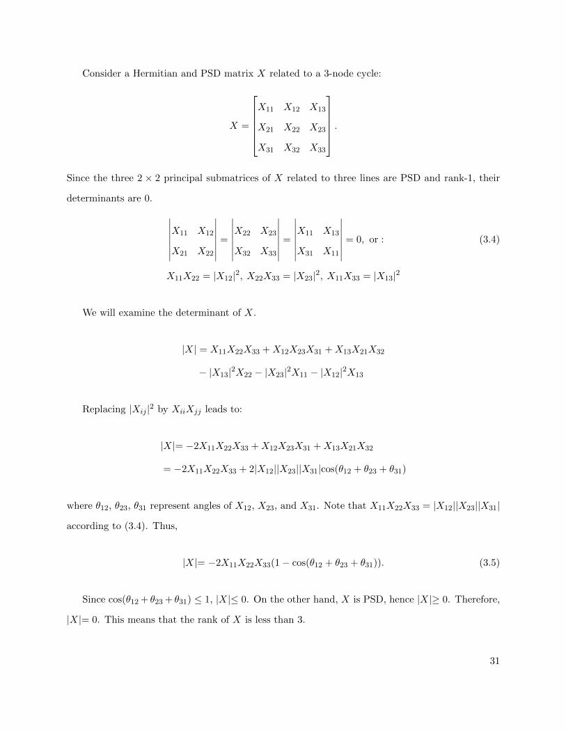
Consider a Hermitian and PSD matrix X related to a 3-node cycle:

X =

X11 X12 X13

X21 X22 X23

X31 X32 X33

.

Since the three 2 × 2 principal submatrices of X related to three lines are PSD and rank-1, their

determinants are 0. ∣∣∣∣∣∣∣X11 X12

X21 X22

∣∣∣∣∣∣∣ =

∣∣∣∣∣∣∣X22 X23

X32 X33

∣∣∣∣∣∣∣ =

∣∣∣∣∣∣∣X11 X13

X31 X11

∣∣∣∣∣∣∣ = 0, or : (3.4)

X11X22 = |X12|2, X22X33 = |X23|2, X11X33 = |X13|2

We will examine the determinant of X.

|X| = X11X22X33 +X12X23X31 +X13X21X32

− |X13|2X22 − |X23|2X11 − |X12|2X13

Replacing |Xij |2 by XiiXjj leads to:

|X|= −2X11X22X33 +X12X23X31 +X13X21X32

= −2X11X22X33 + 2|X12||X23||X31|cos(θ12 + θ23 + θ31)

where θ12, θ23, θ31 represent angles of X12, X23, and X31. Note that X11X22X33 = |X12||X23||X31|

according to (3.4). Thus,

|X|= −2X11X22X33(1− cos(θ12 + θ23 + θ31)). (3.5)

Since cos(θ12 + θ23 + θ31) ≤ 1, |X|≤ 0. On the other hand, X is PSD, hence |X|≥ 0. Therefore,

|X|= 0. This means that the rank of X is less than 3.

31

The sum of angles is found to be 0 since |X|= 0 enforces the following constraint.

cos(θ12 + θ23 + θ31) = 1⇒ θ12 + θ23 + θ31 = 0

This means that cycle (1, 2), (2, 3), (3, 1) satisfies the SOCP exactness condition (3.3b). Therefore,

based on the sparse convex relaxation formulation in (2.7), to have an exact solution, we only need

to enforce 2× 2 submatrices corresponding to all lines rank-1.

We will implement this requirement in convex iteration.

3.3.3 Principle of Convex Iteration

Convex iteration has been applied to SDP OPF to achieve exact solutions in [61, 62]. We will

briefly review convex iteration principle in this section.

For a n× n Hermitian PSD matrix, its trace equals the sum of all its eigenvalues.

Tr(X) =

n∑i=1

λi, λ1 ≥ λ2 ≥ · · · ≥ λn ≥ 0 (3.6)

where λi are the eigenvalues of X; Tr(·) is the “Trace” calculation. If X is rank-1, then all

eigenvalues except λ1 is zero. Thus:

Tr(X)− λ1 = 0. (3.7)

The maximum eigenvalue λ1 can be obtained through the following equation [64]:

λ1 = Tr(Xu1uH1 ) (3.8)

where u1 is the normalized eigenvector correspond to λ1. Thus, combining (3.7) and (3.8) leads to:

Tr(X(I − u1uH1 )) = 0 (3.9)

Define W , I − u1uH1 . If Tr(XW ) = 0, then X is rank-1. Thus by adding Tr(XW ) as a

penalty term on the objective function of the SOCP formulation, we may enforce X to be rank-1.

32

Note that W is also a variable. This makes the problem a bilinear problem. To solve this

bilinear problem, iterative approach can be implemented. Denote the problem including rank-1

penalty term as F (X,W ) whose objective function includes an additional term ωTr(XW ) (ω is

the penalty factor). We may fix W to solve a convex problem and find X. Then for the given X,

we may find W . Below is the iterative procedure:

problem 1: F (X,W ∗) problem 2: F (X∗,W )

where W ∗ is the solution of the problem 2; X∗ is the solution of the problem 1. Consider our

derivation from (3.6) to (3.9), it implies that for a fixed X∗, W can be found through eigenvalue-

based decomposition of X∗.

X∗ = UΛUH (3.10)

where Λ is a diagonal matrix with its elements eigenvalues, U is a unitary matrix, and its columns

are the eigenvectors of X∗, i.e., U = [u1, u2, . . . , un]. Thus, problem 2 for iteration procedure is

equivalent to:

W = UUH − u1uH1 , ⇒W = U(:, 2 : n)U(:, 2 : n)H (3.11)

3.3.4 Sparse Implementation

Further, we seek sparse matrix-based implementation. The sparse convex relaxation solver does

not give the full matrix X. According to Theorem 1, for the 3-node cycle-based convex relaxation,

we only need to enforce all 2× 2 submatrices related to lines and virtual lines rank-1 to achieve the

exactness. Therefore, the rank penalty term Tr(XW ) can be replaced by:

∑i∈AL

Tr(X(i)W (i)) (3.12)

where AL is the set of all lines, including original lines and virtue lines, Xi is the ith 2×2 submatrix

and W i can be found based on Xi using (3.11).

During the iterative procedure, some Tr(X(i)W (i)) term might not keep monotonic decreasing.

This may lead to the increase of the ranks of those submatrices. To keep the submatrices rank-1

33

once they have reached rank-1 during iteration, we implement the following constraints to problem

1:

Tr(X(i)W (i)) ≤ ε i ∈ DL (3.13)

where ε is tolerance, DL is the set for all submatrices that have achieved rank-1. The equivalent

form of this constraint has been adopted in [62].

Our experiments show that this constraint is capable to decrease the iterations for large size

cases. E.g. for nesta case1354 pegase and ω = 1000, with constraint (3.13), convex iteration can

converge at 3 steps; without constraint (3.13), convex iteration can not converge after 10 steps.

The formulation of 3-node based convex iteration is defined as problem 1 and problem 2.

We define the problem 1 as the following equations:

min f(Pg) + ω∑i∈AL

Tr(X(i)W ∗(i)) (3.14)

s.t. Constraints (2.6) (2.7b) ∼ (2.7h)

Tr(X(i)W ∗(i)) ≤ ε i ∈ DL

For all cliques MC

X(i) 0 i ∈ SMC

We define the problem 2 as the following equations:

W ∗(i) = U (i)(:, 2)U (i)(:, 2)H i ∈ AL (3.15)

where U (i) is obtained through the eigenvalue decomposition of X∗(i): X∗(i) = U (i)Λ(i)U (i)H .

The initial values of the iteration can be provided by the solution of Formulation (2.7).

3.4 Nonlinear Rank-1 Formulation

3.4.1 2× 2 Minor-based Rank-1 Constraints

To implement exactness constraints, we convert the constraints in (3.1) to minor constraints [22].

The reformulation is based on Proposition 3.1 in [22]: a PSD matrix X is rank 1 if and only if all

34

its 2× 2 minors are zeros and the diagonal elements of X are non-negative. Note a m×m minor of

the matrix X ∈ Cn×n is defined as the submatrix of X by deleting n−m rows and n−m columns.

For example, suppose that for an Hermitian X, rows except i, l and columns except j, k are

eliminated. The resulting minor constraint is as follows

∣∣∣∣∣∣∣Xij Xik

Xlj Xlk

∣∣∣∣∣∣∣ = 0

⇒ XijXlk −XikXlj = 0

Separating the real and imaginary parts leads to:

⇒

RijRlk − IijIlk −RljRik + IljIik = 0

IijRlk −RijIlk − IljRik −RljIik = 0

(3.16)

Thus we may find all 2×2 minors of the SDP relaxation’s decision variable X. The challenge is

that the number of minors is large. The total number of minor constraints in terms of X is C2nC

2n.

Among them, C2n are the number of the principal minors as shown in (3.2a). These minors can be

expressed in R and I and there are total C2n constraints in the real domain. The rest minors are non-

principal minors and each can be separated into two constraints in the real domain. Considering

the Hermitian matrix’s feature (XT = X∗), we will have C2nC

2n−C2

n2 constraints to represent the

non-principal 2× 2 minors in the complex domain, or C2nC

2n − C2

n non-principal minor constraints

in the real domain. Note that the principal minor constraints include the exactness constraints

for every lines. Therefore, the total number of constraints in real-domain related to all minors is

C2nC

2n. For a 10-node system, this number is 2025.

Instead of dealing with the full matrix X, we now examine the SOCP exactness conditions.

The first condition (3.2a) is related to each line. For a branch connecting Bus i and Bus j, the

exactness condition is to have the principal minor related to i and j be zero. The next condition

(3.2b) is the cycle constraint which should be enforced for every cycles.

In the following, we will show the cycle constraint can be replaced by non-principal minor

constraints of each embedded 3-node cycle. There are three steps to lead to the conclusion. The

35

4

3

2

5

7

9

1

6

8

Figure 3.1: One chordless cycle become 3-node cycles with virtual lines.

first step is to show an n-node cycle can be decomposed into (n− 2) 3-node cycles, the second step

is to show that the exactness conditions in (3.2a) and (3.2b) for a 3-node cycle indeed guarantees a

PSD rank-1 matrix. Hence the conditions can be replaced by a set of 2× 2 minor constraints. The

third step is to show these minor constraints can be expressed as 9 quadratic equality constraints

in the real domain.

3.4.1.1 The First Step: n-node Decomposition

With (n−3) virtual lines, any chordless cycle of n nodes can be decomposed into (n−2) 3-node

cycles. The cycle constraint of the chordless cycle will be replaced by (n − 2) cycle constraints

related to those 3-node cycles.

Fig. 3.1 shows one example power network for the decompose strategy. Three virtual lines are

added in the chordless cycle 4 → 9 → 8 → 7 → 6 → 5 → 4. There are now four 3-node cycles

presented: 4, 5, 6, 4, 6, 7, 4, 7, 8, and 4, 8, 9. In power grids, adding virtual lines is similar

to claim that any two nodes without direct line connection can be viewed as connected through a

line with infinite impedance. The numbers of virtual lines added for a n-node cycle is (n− 3) and

the number of the resulting 3-node cycles is (n− 2).

Obviously, if all 3-node cycles satisfy the cycle constraint (3.2b), the original cycle condition

can also be satisfied.

36

3.4.1.2 The Second Step: Exactness Conditions Conversion

Notate a 3× 3 Hermitian matrix corresponding to a 3-node cycle as Xc. We will show that the

exactness conditions for SOCP relaxation (3.2) related to a 3-node cycle is indeed equivalent to the

corresponding matrix Xc being PSD and rank-1.

Xc =

Xc11 Xc12 Xc13

Xc21 Xc22 Xc23

Xc31 Xc32 Xc33

Its exactness condition is shown as follows.

Xcii ≥ 0, i = 1, 2, 3 (3.17a)

|Xcij |=√XciiXcjj , (i, j) ∈ (1, 2), (2, 3), (3, 1) (3.17b)

6 Xc12 + 6 Xc23 + 6 Xc31 = 0 (3.17c)

(3.17b) indicates that all 2× 2 principal minors equal to 0:

Xc11Xc22 = |Xc12|2= |Xc21|2

Xc22Xc33 = |Xc23|2= |Xc32|2

Xc11Xc33 = |Xc13|2= |Xc31|2

(3.18)

Consider a non-principal minor M in Xc such as:

M = det

Xc21 Xc23

Xc31 Xc33

= Xc21Xc33 −Xc23Xc31

= |Xc21||Xc33|6 Xc21 − |Xc23||Xc31|(6 Xc23 + 6 Xc23)

37

According (3.18) and (3.17c), we can derive:

|Xc21||Xc33|= |Xc23||Xc31|

6 Xc21 = 6 Xc23 + 6 Xc23

⇒ |Xc21||Xc33|6 Xc21 = |Xc23||Xc31|(6 Xc23 + 6 Xc23)

⇒ M = 0

Through the similar processes, we can find all non-principal minors are zeros. Since all 2×2 minors

are 0, the rank of Xc is less than 2. And the diagonal components of Xc are all greater than 0.

Hence Xc is PSD and rank-1.

3.4.1.3 The Third Step: Constraints Reformulation

Basing on the previous step and the Proposition 3.1 [22], for each 3-node cycle, the exactness

condition or Xc is PSD and rank-1 can be replaced by a set of quadratic minor constraints. The

minor constraints of Xc can be expressed as constraints (3.19g).

As a summary, for a power grid that has been decomposed into lines (the set is notated as L),

virtual lines (notated as LV), and 3-node cycles (notated as Ψ), there will be |L|+|LV | constraints

related to the principal minors, and 6 × |Ψ| constraints related to non-principal minors. Take the

example shown in Fig. 3.1, the system has a total 9 lines with one 6-node chordless cycle. Three

virtual lines are added 4 − 6, 4 − 7, 4 − 8 to decompose the chordless cycle into 4 3-node cycles.

The system’s exactness constraints consist of 12 constraints related to the 12 principal minors

corresponding to 12 lines (9 lines and 3 virtual lines) and 6× 4 related to the non-principal minors.

Total, there are 36 quadratic equality constraints.

38

R2ij + I2ij = RiiRjj , (i, j) ∈ (1, 2), (2, 3), (3, 1) (3.19a)

R12R23 − I12I23 −R22R13 = 0, (3.19b)

I12R23 +R12I23 −R22I13 = 0, (3.19c)

R23R13 + I23I13 −R33R12 = 0, (3.19d)

I23R13 −R23I13 +R33I12 = 0, (3.19e)

R13R12 + I13I12 −R11R23 = 0, (3.19f)

I13R12 −R13I12 −R11I23 = 0. (3.19g)

3.4.2 Rank-1 PSD Matrix-Based Nonlinear Programming Formulation

In Section 3.4.1, the exactness conditions have been converted to quadratic equality constraints.

A nonlinear programming problem can now be formulated with those constraints. The next step is

to identify cycles in a power network and decompose any chordless cycle with size greater than 3

into 3-node cycles. With all virtual lines and 3-node cycles identified, the nonlinear programming

formulation can be derived.

3.4.2.1 Cycle Basis Identification

A cycle basis of a graph is the set of cycles with each cycle having only one of its edges common

with the spanning tree of the graph. We use the cycle identification algorithm in [54] to identify

the cycles. A MATLAB based toolbox [55] is applied to find a cycle basis. The algorithm first

searches a minimal spanning tree of the network and then adds the rest of the lines back one by

one. Each added line will be considered as a token to identify one cycle. For example, consider the

five buses network in Fig. 3.2, the set of the lines is L = (1, 2), (2, 3), (3, 4), (4, 5), (5, 1), (4, 1). To

identify its cycles, first the cycle identification algorithm will start from the minimal spanning tree

in Fig. 3.3. This spanning tree contains lines (1, 2), (2, 3), (1, 4), (1, 5). Next, the remaining lines

are added back one by one. After adding (3, 4), we obtain a cycle ca = 1− 2− 3− 4− 1. After

adding (4, 5), we get a cycle cb = 1− 4− 5− 1.

39

1 2 3

45

1

23

4

5

6

Figure 3.2: Five-bus test case with two cycles. Cycle a: nodes 1, 2, 3, 4, lines(1, 2), (2, 3), (3, 4), (4, 1); Cycle b: nodes 1, 4, 5, lines (1, 4), (4, 5), (5, 1).

0.5 1 1.5 2 2.5 3 3.50.5

1

1.5

2

2.5

3

3.5

1

2

3

4 5

Figure 3.3: Spanning tree of the five-bus test system.

3.4.2.2 Nonlinear Programming Problem Formulation

Through the cycle identification algorithm and the graph decomposition process, we obtain a

set of virtual lines and 3-node cycles. The set of all lines including virtual lines are notated as

Lch = LV ∪ L. The proposed rank-1 nonlinear programming formulation is shown in the problem

(3.20).

This problem is a quadratically constrained quadratic program (QCQP) problem with quadratic

equality constraints (3.20h) to (3.20n). The problem can be solved by nonlinear programming

solvers, e.g., IPOPT.

40

Compared with MATPOWER, the decision variables in (3.20) are no longer voltage phasors.

Instead, R and I can be initialized using the solution of the PSD matrix X from a SDP relaxation

ACOPF solver developed in [65].

min∑k∈G

C2kP2gk + C1kPgk + C0k (3.20a)

P gi − Pdi =

∑j∈Adji

(GijRij −BijIij), i ∈ N (3.20b)

Qgi −Qdi =

∑j∈Adji

(−GijIij −BijRij), i ∈ N (3.20c)

|Sij(Rii, Rij , Iij)|≤ Smaxij , (i, j) ∈ L (3.20d)

Pmingi ≤ Pgi ≤ Pmax

gi , i ∈ G (3.20e)

Qmingi ≤ Qgi ≤ Qmax

gi , i ∈ G (3.20f)

(V mini )2 ≤ Rii ≤ (V max

i )2, i ∈ N (3.20g)

R2ij + I2ij = RiiRjj , (i, j) ∈ Lch (3.20h)

For each 3 nodes cycle c = i, j, k ∈ Φ

RijRjk − IijIjk −RjjRik = 0, (3.20i)

IijRjk +RijIjk −RjjIik = 0, (3.20j)

RjkRik + IjkIik −RkkRij = 0, (3.20k)

IjkRik −RjkIik +RkkIij = 0, (3.20l)

RikRij + IikIij −RiiRjk = 0, (3.20m)

IikRij −RikIij −RiiIjk = 0. (3.20n)

3.4.3 Voltage Recover Techniques

The solution from (3.20) is a set of Rii, Rij , and Iij , or partial information of a PSD matrix

X. Voltage vectors can be recovered from the decision variables R and I. Rii will be found for

41

every bus. Rij and Iij are related to all lines and virtual lines. we implement a voltage recovery

method [6] through visiting the spanning tree of the network.

First, we define the phase angle of voltage phasor at the reference node as 0. We identify the

spanning tree of the power network, and define path from the reference node to the node i as Pi.

Then the voltage phasor at any node i can be recovered through the following equations.

Vi =√Rii

θi = −∑

(j,k)∈Pi

6 (Rjk − jIjk)

3.5 Case Studies

In this section, we presented the case studies for the two proposed algorithms. First, the 3-node

cycle-based convex iteration algorithm is tested on some cases which are selected from the Table

2.2. These cases shown relatively large gaps. The converge process of the rank errors are plotted

for the ”case9mod” and ”nesta case300 ieee”. Second, we tested the nonlinear rank-1 formulation

on two sets of cases. The first set of cases are chosen from the NICTA test archive [57]. Gaps

of these cases are small or zeros. The second set of cases are special cases which are modified to

have large gaps. These cases are selected from the test achieves which are provided by [17] and [5].

The related results are listed in the Table 3.2 and 3.3 respectively. Our numerical experiments are

conducted on an Intel(R) Xeon(R) CPU E5-2698 v3 @ 2.30 GHZ (2 processors) computer. All

solvers are implemented in MATLAB 2017a-based CVX platform [58].

3.5.1 Rank-1 Solution Through Convex Iteration

We tested 3-node cycle-based convex iteration method on several non-zero gap cases. In the

experiments, we keep ε = 10−5 used in (3.13) for all cases. Commercial solver Mosek 7.1.0.12 are

called in the script to complete the computation. The results are listed in Table 3.1. Column

Nlines is the sum of the numbers of lines and virtual lines in a graph; Niter is the number of

iterations. In this Table, we apply maximum active and reactive power mismatch to show the

feasibility of the solution, where superscript before means before convex iteration, and after means

after convex iteration. The mismatches are calculated through the power balancing equations using

42

the voltage phasor vector recovered from the solution of a sparse matrix X, where superscript sol

means the solutions directly from Solver C with or without convex iteration; superscript rec means

the solutions obtained through the recovered voltage phasors after the solutions from the proposed

solver. V rec and θrec are the magnitude and angle of the recovered voltage phasor vector. The gap

is defined as: Gap = UB−LBUB × 100%, where UB is the upper bound which is calculated through

MATPOWER; in Table 3.1, LB is calculated by the convex iteration solver.

Table 3.1: Convex iteration results

case UB gap(%) Nlines Niter MaxRank P beforemis Qbefore

mis P aftermis Qafter

mis ω

nesta case5 pjm 17551.89 0.00 7 2 1 0.57 2.17 6.27e-6 1.46e-5 28000nesta case30 fsr api 372.14 0.08 55 5 1 6.89e-2 3.71e-2 3.81e-5 5.54e-5 1210

nesta case118 ieee api 6383.57 0.00 252 6 1 9.26 4.12 4.13e-4 5.25e-4 560nesta case118 ieee 3689.92 0.00 252 4 1 5.80e-1 6.55e-1 2.36e-4 1.90e-4 22nesta case300 ieee 16891.28 0.00 602 6 1 8.12e-1 4.64e-1 1.45e-4 1.87e-4 1000

nesta case1354 pegase 74064.11 0.00 2408 3 1 9.73e-1 6.61e-1 5.27e-4 2.05e-3 821.5case9mod 4267.07 22.89 12 18 1 7.49e-3 2.59e-1 2.66e-9 1.03e-7 1e6

case39mod1 11221.00 0.00 67 19 1 9.92e-2 1.73 1.38e-6 1.53e-5 1.98e5case300mod 378540.50 0.00 602 21 1 7.13 1.79 5.95e-5 5.71e-4 3.91e4

The voltage vector recovering method in [44] is adopted in this project. First, we define the

phase angle of the voltage phasor at the reference node as 0; next, we identify the spanning tree

of the power network, and define the unique path from the reference node to the node i as Pi; then

the voltage phasor at any node i can be recovered through the following equations.

V reci =

√cii, θreci = −

∑(j,k)∈Pi

6 (cjk − jsjk)

The results in Table 3.1 show that the proposed convex iteration is capable of decreasing max-

imum rank of submatrices. In Fig.3.4 we show that the rank error represented by∑Tr(X(i)W (i))

decreasing for two instances. According to Table 3.1, all 9 instances successfully achieve rank-1 , the

power mismatches are close to 0, and gaps are non-negative. It means the recovered voltage vectors

from the convex iteration solutions are feasible for the original ACOPF, and the objective value is

not worse than the MATPOWER. We noted in Table 3.1, the gap for case9mod case is 22.89% while

MaxRank is one. The reason of this situation is that the case9mod case has multi-local optimal

solutions [5]. The MATPOWER which is based on the interior point method obtained one of the

43

local optimal solution, while the convex iteration solver obtained another optimal solution which

is closer to the global optimal.

2 4 6 8 10 12 14 16 18

Iterations

10-6

10-4

10-2

Ran

k E

rror

case9modnesta_case300_ieee

Figure 3.4: Rank error converging for two instances.

3.5.2 Nonlinear Rank-1 Formulation

In this section, we present the case study results for nonlinear rank-1 formulation. The proposed

nonlinear programming ACOPF formulation was implemented in MATLAB using Yalmip and select

IPOPT as the main solver. The configurations of the IPOPT are: convergence tolerance is 1×10−7;

maximum number of iteration is 10000; update strategy for barrier parameter is “adaptive”; Hessian

information is “limit-memory”; and the other configurations are default.

To obtain the initial point for the nonlinear solver, we solve OPF problems first through a

CVX [66] based sparse SOCP/SDP relaxation solver [65]. The objective value of the SOCP/SDP

solver and the maximal rank of the corresponding PSD submatrices will be given for each test case.

MATPOWER with IPOPT as the solver is used for comparison.

In results tables, the column ”Rank” list the maximal rank of all submatrices for each case.

For each submatrix, rank is counted by considering only the eigenvalues that are greater than the

0.001% of the maximal eigenvalue; N vlines is the number of the virtual lines; N lines is the number

of the original lines; N cycle3 is the number of the 3-node cycles based on the decomposition results.

In Table 3.2, the results show that for all tested standard cases, our formulation provides

the same objective values as those from MATPOWER. In Table 3.3, we listed test results on

44

modified cases. From the table, we can see that for cases with large gaps, the proposed formulation

is capable to obtain the same objective value as MATPOWER. These results indicate that the

proposed formulation can provide similar quality results to the original ACOPF formulation that

is implemented in MATPOWER. Moreover, according the number of 3-node cycles, we can see the

improvement on the number of the added equality constraints. For example, in ”nesta case57 ieee”,

N vlines= 55,N lines= 78, N cycle3= 77, which means the number of the added equality constraints

are 77× 6 + 78 + 55 = 595. This number is much less than C257C

257 = 2547216 which is the number

of the added equality constraints without the decomposition. For the cases from ”case9Tree” to

”case57Tree” in table 3.3, as they are radial networks, we do not add any virtual line on them.

Table 3.2: Test case results

SDP Relaxation Matpower Nonlinear Rank 1 Method

Case Obj Rank %Gap Obj Obj %Diff N vlines N lines N cycle3

nesta case3 lmbd 5789.914 2 0.04 5812.643 5812.643 0.00 0 3 1

nesta case5 pjm 16635.76 2 5.22 17551.891 17551.889 0.00 1 6 3

nesta case9 wscc 5296.685 2 0.00 5296.686 5296.686 0.00 3 9 4

nesta case57 ieee 1143.280 2 0.00 1143.283 1143.283 0.00 55 78 77

nesta case89 pegase 5820.217 2 0.00 5820.387 5820.387 0.00 55 206 173

nesta case118 ieee 3689.495 3 0.01 3692.891 3692.891 0.00 73 179 135

Table 3.3: Special test case results

SDP Relaxation Matpower Nonlinear Rank 1 Method

Case Obj Rank %Gap Obj Obj %Diff N vlines N lines N cycle3

WB5 946.530 2 0.01 946.584 946.584 0.00 1 6 3

case9mod 2753.041 2 10.84 3087.842 3087.842 0.00 3 9 4

case39mod1 10804.055 2 3.72 11221.003 11221.003 0.00 21 46 29

case39mod2 940.341 2 0.15 941.738 941.738 0.00 21 46 29

case9Tree 5335.701 2 52.70 11279.476 11279.476 0.00 0 8 0

case14Tree 11861.899 2 0.59 11932.252 11932.252 0.00 0 13 0

case30Tree 4244.549 2 11.47 4794.313 4794.314 0.00 0 29 0

case39Tree 44868.452 2 0.37 45037.039 45037.042 0.00 0 38 0

case57Tree 10458.099 2 13.58 12100.849 12100.856 0.00 0 56 0

3.6 Conclusion

In this chapter, an efficient convex iteration implementation is also investigated for the proposed

sparse convex solver to achieve exactness or rank-1 solutions. Our experiment results show the

feasibility of the implementation. Moreover, we proposed a nonlinear programming formulation for

45

ACOPF. This formulation is based on decision variables that align with SOCP/SDP relaxation.

The proposed formulation exploits power network sparsity feature and employs a small set of minor

constraints related to all 3-node cycles as equality constraints to enforce rank-1 constraint, so the

solution is exact. Case study results demonstrate the correctness of this formulation.

46

Chapter 4: Benders’ Decomposition for MPC of a Modular Multi-level Converter

4.1 Introduction

3Compared with traditional two-level VSC, multilevel voltage-source converters have much lower

harmonic in the output voltage, which significantly reduces the size of grid side filter [68]. Among

the different multilevel converters, MMC has modular topology and the extensibility for several

hundreds of output voltage levels. Therefore, MMC is ideal for high-voltage high-power applica-

tions, such as HVDC transmission [69], high-voltage motor drives [70], and electric railways [71].

Fig. 4.1 is the topology of a three phase MMC. For an N + 1 level MMC, there are N sub-modules

on each arm of the converter. Each sub-module is a half bridge dc-dc converter. Since the current

flows through different sub-modules at different times, the voltages of sub-modules capacitors vary.

4.1.1 State-of-the-art MMC Switching Schemes

MMC control differs from two-level VSC control in two aspects: 1) switching sequence genera-

tion and 2) the inclusion of circulating current mitigation control. In switching sequence generation,

in two-level VSCs, the output from PWM is the switching sequence directly fed to the gates. In

MMCs, due to the large number of sub-modules, the output of pulse-width modulation or other

types of switching schemes is the number of sub-modules to be turned on at each arm. Which

sub-modules to be turned on then depends on additional sub-module voltage balance consideration.

The PWM switching schemes are also very different from that of two-level VSCs. Phase-disposition

(PD)-PWM and Phase shifted-PWM are often adopted [72]. In MMC’s PWM, there are usually

many carrier signals for the reference sinusoidal signal to be compared to; while in two-level VSC’s

PMW, there is usually one triangular carrier signal.

3This Chapter was published in 2017 North American Power Symposium (NAPS) [67]. Permission is included inthe Appendix A.

47

SM1

SM2

SMN SMN SMN

Vgb

+

-

VSM

T1

T2

SM1 SM1

SM2 SM2

SMN SMN SMN

SM2SM2 SM2

SM1 SM1 SM1

Vc_SM

R0

L0

R0

L0RL

R0

L0

R0

L0

R0

L0

Vgc

Vga

R0

L0

R0

L0

Vdc/2

-Vdc/2

Vcu,a

Iu,a

Il,a

Io,a

+

-

Vcl,a

+

-

Figure 4.1: Three phase MMC topology.

MMC PWM gives only the number of modules to be switched on. To determine which modules

to be switched on, another phase is required: capacitor voltage balancing. A capacitor voltage

balancing block selects the proper sub-modules to be switched.

4.1.2 Our Contributions

As an advanced control method, MPC is very successful on its application for the control of

power converters [25]. Its basic principle is to generate a system dynamic model based minimizing

optimization problem, and provide the solutions to the controller for driving the system to reach

the control target (Generally will be formulated as the objective function in the MPC optimization

problem). A major challenge for implementing MPC on MMC is because the system dynamic

model of MMC is nonlinear with binary terms, in other word, the MPC problem of MMC is a

Mix-integer programming problem which generally is difficult to solve precisely.

In this chapter, we adopt Benders’ decomposition to solve the MPC problem. Our major focus

are the derivation for the MPC problem formulation and its Benders’ decomposition format. In

the case study section, the potential and practicability of the this application are verified, but also

48

0 0.002 0.004 0.006 0.008 0.01 0.012 0.014 0.016

−3

−2

−1

0

1

2

3

Seven level PD−PWM

Time (sec)

0 0.002 0.004 0.006 0.008 0.01 0.012 0.014 0.016

−3

−2

−1

0

1

2

3

Switching signal generated by 7−level PD−PWM

Time (sec)

Figure 4.2: Three-level and Seven-level VSC PD-PWM scheme and switching status. (a)Three-level VSC PD-PMW scheme and switching status of a phase.(b) Seven-level VSC

PD-PWM scheme and switching status of a phase.

revealed some limitations of it. The further discussion about how to overcome these limitation will

be the topic of our next chapter, so it is not included in this one.

The rest of the chapter is organized as follows. Section 4.2 gives the dynamic model of MMC.

Section 4.3 gives the details about the formulation of the MPC problem. And then, its Benders’

algorithm format are derived in Section 4.4. Section 4.5 presents the case study and results. Finally,

the chapter are concluded in Section 4.6.

49

4.2 Dynamic Model of MMC

Fig. 4.1 shows the overall structure of a three-phase MMC consisting of six arms. Subscripts u

and l denote upper and lower arms, respectively. There are N sub-modules and one inductor L0

on each arm. A resistor R0 is inserted to represent the switching loss of the IGBTs on each arm.

The output voltage of each sub-module has two values, Uc (when T1 is connected) and 0 (when

T2 is connected). When the number of sub-modules or the switching frequency is high enough,

the voltage across whole sub-modules in each arm can be considered as continuous. Since the dc

side capacitors are usually big enough, the voltage across the arm can be considered as constant dc

voltage sources. Thus, we can express a single phase-equivalent circuit of a MMC as Fig. 4.3.

Vcu

+

-

L0

L0

R0

R0R L

io

il

iu

idiff

Vdc/2

Vdc/2

O

Vcl

+

-

vo vg

Figure 4.3: Single phase equivalent circuit of MMC.

In Fig. 4.3, iu and il are the arm currents for upper and lower arms; io and vo are the converter

output current and voltage respectively. The circulating current flowing within the converter is

denoted as iz. Since the upper and lower arm are symmetric, ideally both lower and upper arm

currents contain half of the converter output current. Therefore, with KCL, we can get following

equations: iu = iz + io

2

il = iz − io2

⇒

iz = iu+il

2

io = iu − il.(4.1)

50

The voltage across the arm resistance and inductance can be expressed by the arm current.

Therefore, with KVL, we can have the voltage relationship as follow:

vu + iuR0 + L0

diudt = Vdc

2 − vo

vl + ilR0 + L0dildt = Vdc

2 + vo

(4.2)

Considering that the output voltage vo can be written as vg+ioR+Ldiodt and (4.1), by subtracting

the two equations from (4.2) we have:

vu − vl2

+

(R+

1

2R0

)io +

(L+

1

2L0

)diodt

+ vg = 0 (4.3)

It is obvious that the term vu−vl2 in (4.3) drives the output current of the converter, therefore

we name this term as e, which is the inner emf of the converter. We can have an equivalent circuit

of MMC as Fig. 4.4, which is the plant model of inner current control loop of an MMC.

R0 L0

R0 L0

R L

Vgea

Figure 4.4: An equivalent circuit of one phase of MMC.

Adding the two equations in (4.2) leads to the plant model of the circulating current control:

izR0 + L0dizdt

=Vdc2− vu + vl

2. (4.4)

51

Considering Fig. 4.1, since vu and vl are the sum of all sub-module voltages on the correspond

arm, we can express vu and vl through the following equations:

vu =

∑Ni=1 VSMi i on the upper arm

vl =∑2N

i=N+1 VSMi i on the lower arm

(4.5)

For convenient, we name the voltage of the capacitor on each sub-module as vc(i), and the state

of the correspond IGBT as u(i). Apparently, VSMi = vc(i)u(i), combine it with the equation (4.5),

then we have: vu =

∑Ni=1 vc(i) i on the upper arm

vl =∑2N

i=N+1 vc(i) i on the lower arm

(4.6)

4.3 Optimization Problem Formulation

We propose to discretize the continuous dynamic model of MMC which described by (4.1) to

(4.6). It means we consider

diodt

=io(k + 1)− io(k)

h(4.7)

dizdt

=iz(k + 1)− iz(k)

h(4.8)

where h is step size of the discretized signal, k ∈ 1, 2, · · · , T is the index of the time step.

Combining (4.7) and (4.8) respectively with (4.3) and (4.4), then we obtain the following equations:

io(k + 1) = io(k) +h

L+ L02

[−(R+

R0

2

)io(k)− vg(k)− vu(k)− vl(k)

2

](4.9)

iz(k + 1) = iz(k) +h

L

[−R0iz(k) +

Vdc2− vu(k) + vl(k)

2

](4.10)

52

where vu(k) =

∑Ni=1 vc(i, k)u(i, k)

vl(k) =∑2N

i=N+1 vc(i, k)u(i, k)

(4.11)

In (4.11), N is the numbers of switches on one arm, i ∈ 1, 2, · · · , 2N is the index of switches.

We expect to control the MMC output current to track the current reference which is a sinusoidal

waveform. This can be expressed by solving the following optimization problem:

min

T∑k=1

[irefo (k)− io(k)

]2(4.12)

subject to (4.9), (4.10),

vu(k) =

N∑i=1

vc(i, k)u(i, k)

vl(k) =

2N∑i=N+1

vc(i, k)u(i, k)

vc(i, k + 1) =

vc(i, k) + hc · u(i, k)

[io(k)2 + iz(k)

],

i = 1, 2, · · · , N.

vc(i, k) + hc · u(i, k)

[− io(k)

2 + iz(k)],

i = N + 1, · · · , 2N2N∑i=1

u(i, k) = N

u(i, k) ∈ 0, 1

where irefo is our desired current, u(i, k) is the state of the ith switch at the kth time step, vc(i, k)

is the voltage on the ith switch capacitor at the kth time step.

If we replace the binary constraint u(i, k) ∈ 0, 1 by an equality constraint u(i, k)(1−u(i, k)) =

0 with u(i, k) as continuous variable, then this problem can be solved by nonlinear programming

solver fmincon using sequential quadratic programming (SQP) algorithm.

53

4.4 Benders’ Decomposition Formulation

To implement Benders’ decomposition for solving the problem (4.12), we separate the problem

to a master problem and a sub-problem. In the sub-problem problem, the binary variable u is

considered as fixed values. Therefore the sub-problem could be solved as a linear programming

problem. Iteratively, the dual variables which are solved from the sub-problem will be used to

generate the Benders’ cuts and add them to the master problem. And then, the solution of u from

the master problem will be returned to the sub-problem. This iteration process will be repeated

until the stop criteria are met.

4.4.1 Subproblem

In our case, decision variables in the sub-problem are: io, iz, vu, vl, and vc, and define any given

u as u, its primal problem could be expressed as follow:

min

T∑k=1

[irefo (k)− io(k)

]2(4.13)

subject to (4.9), (4.10)

vu(k) =

N∑i=1

vc(i, k)u(i, k)

vl(k) =2N∑

i=N+1

vc(i, k)u(i, k)

vc(i, k + 1) =

vc(i, k) + hc · u(i, k)

[io(k)2 + iz(k)

]i = 1, 2, · · · , N.

vc(i, k) + hc · u(i, k)

[− io(k)

2 + iz(k)]

i = N + 1, · · · , 2N.

To generate the Benders’ cuts, we need to find dual variables which correspond with the con-

straints that include u. To achieve this, first we define a Lagrangian function to aggregate the

54

objective function and the constraints that are related to u.

L =

T∑k=1

[irefo (k)−io(k)

]2+∑i

∑k

λ1(i, k)

vc(i, k+1)−vc(i, k)− h

cu(i, k)

[io(k)

2+iz(k)

]+∑i

∑k

λ2(i, k)

vc(i, k+1)−vc(i, k)− h

cu(i, k)

[− io(k)

2+iz(k)

]

+∑k

λ3(k)

[vu(k)−

N∑i=1

vc(i, k)u(i, k)

]

+∑k

λ4(k)

[vl(k)−

2N∑i=1+N

vc(i, k)u(i, k)

].

The partial dual of the original problem could be formulated as follows.

maxλ

minL

subject to (4.9), (4.10)

4.4.2 Cuts Introduced by the Subproblem

We formulate cuts in the following inequality constraint:

µ ≥ vlLB[ul(i, k)

]+∑k

∑i

gl(i, k)[u(i, k)− ul(i, k)

](4.14)

where vLB is the optimal solution of the subproblem while u = u, l is the index of the cuts, matrix

g is defined as:

g =

∂L(λ1,λ2,λ3,λ4)

∂u(1,1) · · · ∂L(λ1,λ2,λ3,λ4)∂u(1,T )

.... . .

...

∂L(λ1,λ2,λ3,λ4)∂u(2N,1) · · · ∂L(λ1,λ2,λ3,λ4)

∂u(2N,T )

Thus

g(i, k) = −λ1(i, k)h

ciu(k)− λ2(i, k)

h

cil(k)

−λ3(k)vci(k)− λ4(k)vc,i+N (k)

55

4.4.3 Master Problem

Associating Benders’ cuts, the master problem can be written as the problem (4.15). Apparently,

problem (4.15) is a mixed integer linear programming problem which can be solved by gurobi or

Mosek. In the Benders’ algorithm, the values of the objective function for the master problem are

the upper bounds of the optimal values for the original problem. And the values of the objective

function for the sub-problem are the lower bounds. Therefore, through the iteration, if the objective

function’s values of the master problem and sub-problem are close enough to reach a stop criteria,

we can consider the optimal solutions are found. Generally, the criteria are defined as:

ε >= |Vmas − Vsub|

where Vmas is the objective function’s value of the master problem, Vsub is the objective function’s

value of the sub-problem, and ε is a fixed small value.

min µ (4.15a)

subject to2N∑i=1

ui(k) = N (4.15b)

ui(k) ∈ 0, 1 (4.15c)

µ ≥ vlLB[ul(i, k)

]+∑k

∑i

gl(i, k)[u(i, k)− ul(i, k)

](4.15d)

4.5 Case Study

In this section, we select a N = 4 MMC as the platform for testing the effectiveness of the

Benders’ algorithm. The parameters of the MMC and MPC time step size are listed in Table 4.1.

Matlab CVX toolbox with Mosek solver are applied to solve its master and sub-problem. Moreover,

we set the stop criteria constant ε = 1×10−5. For comparison, we also develop a group of MATLAB

codes to solve the problem (4.12) via fmincon function based SQP method, and separately list the

56

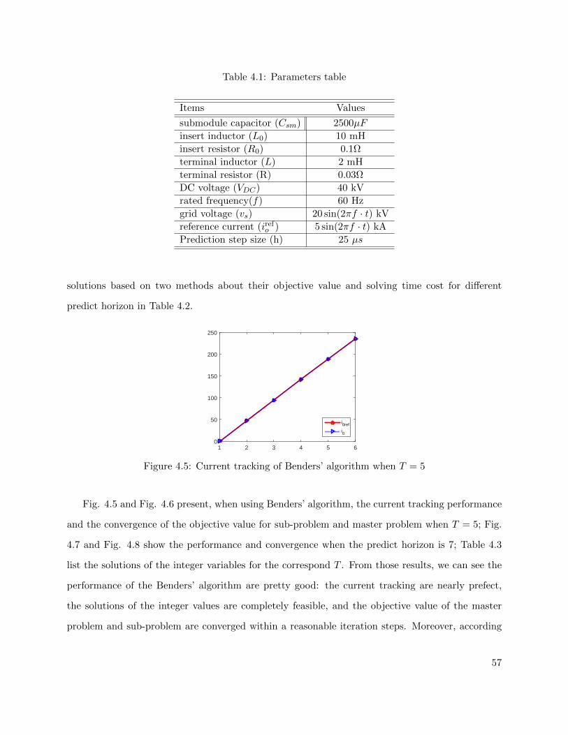
Table 4.1: Parameters table

Items Values

submodule capacitor (Csm) 2500µF

insert inductor (L0) 10 mH

insert resistor (R0) 0.1Ω

terminal inductor (L) 2 mH

terminal resistor (R) 0.03Ω

DC voltage (VDC) 40 kV

rated frequency(f) 60 Hz

grid voltage (vs) 20 sin(2πf · t) kV

reference current (irefo ) 5 sin(2πf · t) kA

Prediction step size (h) 25 µs

solutions based on two methods about their objective value and solving time cost for different

predict horizon in Table 4.2.

1 2 3 4 5 60

50

100

150

200

250

i0ref

i0

Figure 4.5: Current tracking of Benders’ algorithm when T = 5

Fig. 4.5 and Fig. 4.6 present, when using Benders’ algorithm, the current tracking performance

and the convergence of the objective value for sub-problem and master problem when T = 5; Fig.

4.7 and Fig. 4.8 show the performance and convergence when the predict horizon is 7; Table 4.3

list the solutions of the integer variables for the correspond T . From those results, we can see the

performance of the Benders’ algorithm are pretty good: the current tracking are nearly prefect,

the solutions of the integer values are completely feasible, and the objective value of the master

problem and sub-problem are converged within a reasonable iteration steps. Moreover, according

57

1 2 3 4 5-350

-300

-250

-200

-150

-100

-50

0

50

value of subproblemvalue of master problem

Figure 4.6: Convergence of the objective value for the master problem and sub-problem whenT = 5.

the data in Table 4.2, which is proposed to compare the solutions of the problem (4.12) by Benders’

algorithm and SQP method, we can see the Benders’ algorithm has some obvious advantages than

SQP method.

0 1 2 3 4 5 6 7 80

50

100

150

200

250

300

350

i0ref

i0

Figure 4.7: Current tracking of Benders’ algorithm when T = 7.

Table 4.2: Results comparison of Benders’ decomposition and SQP algorithm

T Nonlinear Benders

Obj T (sec) UB LB T (sec)

5 2.90 11.19 1.11e-16 1.11e-16 0.77

7 7.24 39.96 2.80e-6 2.80e-6 1.87

10 22.28 40.70 0.16 -0.72 56.61

58

1 3 6 9 12 15-1200

-1000

-800

-600

-400

-200

0

value of subproblemvalue of master problem

Figure 4.8: Convergence of the objective value for the master problem and sub-problem whenT = 7.

Table 4.3: Binary solution

T = 5 T = 7

0 1 0 0 1 0 1 1 0 0 1 10 0 1 1 0 0 0 0 0 1 1 01 0 0 1 0 1 0 0 1 1 0 10 1 1 0 0 1 0 1 0 1 1 11 0 0 1 0 1 1 1 1 1 0 11 0 1 0 1 1 1 0 0 0 0 01 1 1 1 1 0 1 1 1 0 1 00 1 0 0 1 0 0 0 1 0 0 0

However, from the data in Table 4.2 when T = 10, we can see, after more time cost than the

SQP method, the difference between the master problem and sub-problem still can not reach the

stop criteria. In fact, when T = 10, even spend more than one hour to run the Benders’ algorithm

to 70 iteration steps, the convergence result can not be changed significantly and not reach the stop

criteria. The reasons of this situation are because the optimal value of the sub-problem can not

be guaranteed to decrease during the iteration [73], and complexity of master problem is increased

two much while add too much cuts on it. Fortunately, from Fig. 4.10 and Fig. 4.9, we can see the

tendency of convergence is obvious for the master problem and sub-problem. Thus, we can expect,

if provide longer enough time for iteration, or solve those two problems that we mentioned before,

Benders’ algorithm will be practicable when T ≥ 10.

59

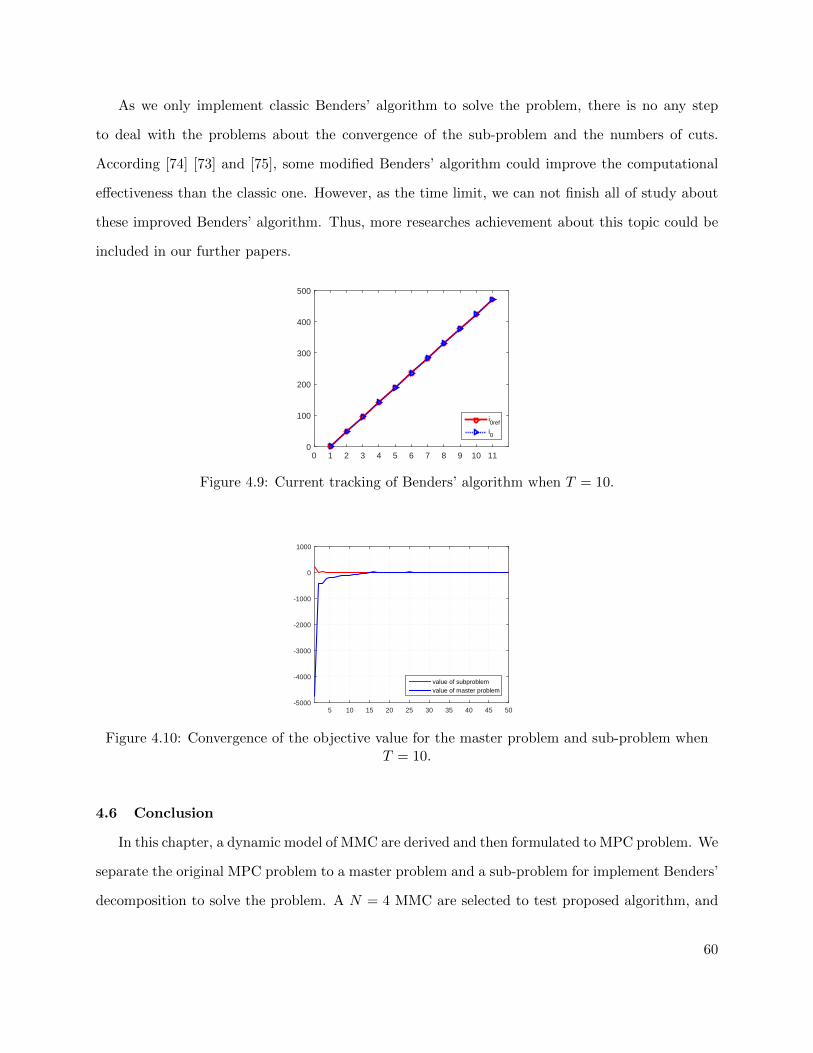
As we only implement classic Benders’ algorithm to solve the problem, there is no any step

to deal with the problems about the convergence of the sub-problem and the numbers of cuts.

According [74] [73] and [75], some modified Benders’ algorithm could improve the computational

effectiveness than the classic one. However, as the time limit, we can not finish all of study about

these improved Benders’ algorithm. Thus, more researches achievement about this topic could be

included in our further papers.

0 1 2 3 4 5 6 7 8 9 10 110

100

200

300

400

500

i0ref

i0

Figure 4.9: Current tracking of Benders’ algorithm when T = 10.

5 10 15 20 25 30 35 40 45 50-5000

-4000

-3000

-2000

-1000

0

1000

value of subproblemvalue of master problem

Figure 4.10: Convergence of the objective value for the master problem and sub-problem whenT = 10.

4.6 Conclusion

In this chapter, a dynamic model of MMC are derived and then formulated to MPC problem. We

separate the original MPC problem to a master problem and a sub-problem for implement Benders’

decomposition to solve the problem. A N = 4 MMC are selected to test proposed algorithm, and

60

the solutions for different predict horizon are displayed and compared with the solutions by SQP.

According the results, Benders’ decomposition has great performance on solving the low horizon

MPC problem and much better than SQP method. But for longer horizon (T ≥ 10), even it has

presented potential to solve the problem, the algorithm still need more improvement to reduce the

computing cost.

61

Chapter 5: Security Constrained DC OPF Considering Generator Responses

5.1 Introduction

4Security constrained OPF(SCOPF) is an extension of OPF considering only pre-contingency or

base case constraints. Its purpose is to find an operation point to optimize an objective function at

base case, while the post-contingency constraints can all be satisfied. The formulation of SCOPF has

two major categories: 1) preventive SCOPF (PSCOPF) [77]; 2) corrective SCOPF (CSCOPF) [29].

In PSCOPF, all control variables are considered without rescheduling except the automatic response

of the system.

In conventional formulation of preventive security constrained OPF, contingencies related to

generator outages are ignored [32] [33] [34]. Or, same operating conditions are assumed for genera-

tors in the pre- and post- contingency [78] [79]. On the other hand, in practical situations, generator

outage is common and the system may assume a very different response compared to the related

to line outages [80]. With generator outages, online generators have to re-dispatch to compensate

the power loss. Their responses are governed by their automatic generator control (AGC) setting.

A generator’s post contingency response is illustrated in Fig. 1.2, where Pmaxg and Pmin

g are

the upper and lower limits of the generator active power output respectively; P(0)gi is the generator

power in pre-contingency state; P(k)g is the generator power in post-contingency state; ∆(k) is the

active power imbalance in the system; α is the participation factor corresponding to the slop; Three

feasible regions are denoted in the figure.

Modeling the non-convex generator response characteristics has been carried out in the liter-

ature. In [81] and [35], the authors assume the generator response in post-contingency always

follow their predefined participation factors, i.e. only region (2) is considered. This formulation

could efficiently simplify the problem, because the generator responses are formulated as a set of

4This Chapter was published in Electric Power Systems Research [76]. Permission is included in the Appendix A.

62

linear constraints. However, due to the omission of feasible regions (1) and (3), the solutions may

be more costly. Alternatively, mixed integer programming (MIP) formulation has been designed

in [37] and [38]. The generator response constraint is formulated as a set of MILP constraints based

on big-M technique. The major disadvantage if this method is well-known disadvantage related to

big-M formulation, i.e., the difficulty of finding a suitable value of M.

Another major challenge to solve SCOPF with generator response constraints is the large size of

the problem. Even we only consider the ”N-1” criterion, the computation cost of the SCOPF with

all contingencies considered could be too high. To address this issue, decomposition techniques

have been implemented to reduce the computing cost. For example, alternating direction method

of multipliers (ADMM)-based decomposition is adopted in [81], [36], [31] to decompose the original

SCOPF problem into one master problem and several sub-problems based on each contingency.

The ADMM methods are heuristic methods to handle non-convexity and the solution from

ADMM dose not guarantee global optimum. Hence, this chapter focuses on investigating a more

efficient MIP and solving strategy.

The contribution of this part is two fold. 1) A bilinear MIP formulation is designed to model

generator post-contingency responses. The proposed model accurately represents the generator

response characteristics. 2) An efficient Benders’ decomposition is designed to decompose the

bilinear MIP problem. Various benders’ decomposition strategies were investigated in this research.

Through preserving bilinear expressions related to the base case power generation while relaxing the

rest bilinear expressions via McCormick envelop, we designed a Benders’ decomposition strategy

that yields to efficient solving.

5.2 DC-PSCOPF Formulation

The mathematical formulation of security constrained DCOPF is as follows:

min f(x(0), u(0)) (5.1a)

s.t. g(k)(x(k), u(k)) = 0 k ∈ C (5.1b)

h(k)(x(k), u(k)) ≤ 0 k ∈ C (5.1c)

63

where x refers to DC power flow state variables: bus voltage phase angles at each scenario,

u refers the control variables: active power dispatch of each generator at each scenario, C =

(0), (1), . . . , (Nc) is the set for the index of scenarios. If k = 0, the correspond constraints and

variables belong to the base case (pre-contingency).

The decision variables of SCOPF are the base case control actions u(0), state variables x(0) and

contingency case state variables x(k).

The objective function is the total operation cost. Denote the cost coefficients as C2i, C1i, C0i,

the objective function could be defined as:

f0 =∑i∈Gon

C2i(P(0)gi )2 + C1iP

(0)gi + C0i

where P(0)gi is the i-th generator’s active power dispatch in base case and Gon notates the set of

online generators. The equality (g) and inequality (h) are explained as follows.

5.2.1 Equality Constraints: Power Flow Equations

The following constraints are enforced on all bus i ∈ N for base case and post-contingency

scenarios:

P(0)gi − Pdi =

∑(i,j)∈L

Bij(θ(0)i − θ

(0)j ) i ∈ N (5.2)

P(k)gi − Pdi =

∑(i,j)∈Lk

Bij(θ(k)i − θ

(k)j ) i ∈ N (5.3)

where L and Lk are the set of transmission lines in base case and post-contingency scenarios; P(k)gi

is the generator active power dispatch in post-contingency scenarios; P(k)di is the load at bus i; Bij

is the susceptance of the transmission line from bus i to bus j; θi is the voltage phase angle of bus

i.

5.2.2 Inequality Constraints: Component Limits

Inequality constraints include transmission line limits, generator power limits, and others. Eqs.

(5.4) and (5.5) notate transmission line flow limits. Eqs. (5.6) and (5.7) notate generator power

64

limits. Eqs. (5.8) and (5.9) enforce the reference bus angle to zero.

|Bij(θ(0)i − θ(0)j )|≤ Fmax

ij (i, j) ∈ L (5.4)

|Bij(θ(k)i − θ(k)j )|≤ Fmax

ij (i, j) ∈ Lk (5.5)

Pmingi ≤ P

(0)gi ≤ P

maxgi i ∈ G (5.6)

Pmingi ≤ P

(k)gi ≤ P

maxgi i ∈ Gk (5.7)

θ(0)ref = 0 (5.8)

θ(k)ref = 0 (5.9)

where G(0)on and G(k)on are the sets of generators in base case and post-contingency scenarios; Fmaxij is

the maximum transmission line capacity; Pmingi and Pmax

gi are the lower and upper limits of generator

active power output; θref means the reference bus voltage phase angle.

5.2.3 Generator Post-contingency Response Constraints

When there is a generator outage, the rest of the generators will adjust their outputs based on

their participation factors to make up the lost power. If the total load keeps constant, the load

variation is zero. Thus, the definition of ∆(k) has to be carefully designed to consider both load

variation contingency and generator outage (while load being constant) contingency.

Hence, ∆(k) is defined as total generation change for the set of online generators at kth contin-

gency.

∆(k) =∑i∈Gon

P(k)gi −

∑i∈Gon

P(0)gi (5.10)

P(k)gi = P

(0)gi + α

(k)i ∆(k) (5.11)

where Gon ⊆ G is the set of all online generators at kth contingency, α is the participation factor

and

∑i∈Gon

α(k)i = 1 (5.12)

65

Considering the output limit of generators, (5.11) can not always be complied by generators.

If P(0)gi + α

(k)i ∆(k) is lower than the minimum limit or greater than the maximum limit, generator

should dispatch at its minimum or the maximum at this contingency. The response of the generator

can be illustrated in Fig. 1.2.

Moreover, according to [82], these three region can be described as a piecewise function:

Region (1) : P(k)gi = Pmax

gi (5.13a)

P(k)gi ≤ P

(0)gi + α

(k)i ∆(k) (5.13b)

Region (2) : Pmingi ≤ P

(k)gi ≤ P

maxgi (5.13c)

P(k)gi = P

(0)gi + α

(k)i ∆(k) (5.13d)

Region (3) : P(k)gi = Pmin

gi (5.13e)

P(k)gi ≥ P

(0)gi + α

(k)i ∆(k) (5.13f)

If all generators comply with the above constraints, the problem may be infeasible. Below is

an example. For a system with more than three generators, assume that the post-contingency

generation of G1 is in region (1), but all the other generators are in Region (2), i.e. P(k)g1 =

Pmaxg1 < P

(0)g1 + α

(k)1 ∆(k), and the other generator follow: P

(k)gi = P

(0)gi + α

(k)i ∆(k). In this situation,

Pmaxg1 −P (0)

g1 +∑

i∈Gon α(k)i ∆(k) < ∆(k). So that the power imbalance can not be fully compensated.

To avoid this situation, we set a reference generator in the system. The generator dose not follow

the constraint (5.13).

5.2.4 The MILP Formulation

The piecewise function (5.13) is non-convex. The set of constraints can be formulated via big-M

technique into an MILP formulation is briefly introduced. Since there are three regions, two binary

variables are introduced: ω(k)1i (1 for max limit hitting; 0 for otherwise) and ω

(k)2i (1 for min limit

hitting; 0 for otherwise).

66

Hence, region (1) is represented by (ω(k)1i , ω

(k)2i ) = (1, 0), region (2) is (ω

(k)1i , ω

(k)2i ) = (0, 0) and

region (3) is (ω(k)1i , ω

(k)2i ) = (0, 1).

Pmingi ≤ P

(k)gi ≤ P

maxgi (5.14a)

Pmaxgi − P (k)

gi ≤ (1− ω(k)1i )M (5.14b)

P(k)gi − P

mingi ≤ (1− ω(k)

2i )M (5.14c)

P(k)gi ≤ P

(0)gi + α

(k)i ∆(k) + ω

(k)2i M (5.14d)

P(k)gi ≥ P

(0)gi + α

(k)i ∆(k) − ω(k)

1i M (5.14e)

ω(k)1i + ω

(k)2i ≤ 1

ω(k)1i , ω

(k)2i ∈ 0, 1

• (ω(k)1i , ω

(k)2i ) : (1, 0), (5.14) equivalent to (5.13a) and (5.13b);

• (ω(k)1i , ω

(k)2i ) : (0, 0), (5.14) equivalent to (5.13c) and (5.13d);

• (ω(k)1i , ω

(k)2i ) : (0, 1), (5.14) equivalent to (5.13e) and (5.13f).

M is a large enough constant number. This method is easy to implement, but there is no guaranteed

way to find a appropriate value for M . If M is too small, the equivalent relation between (5.13)

and (5.14) can not be held. If M is too large, it may cause numerical instability for computation.

Based on the MILP formulation, Benders’ decomposition has been proposed in [38].

5.3 The Proposed the Bilinear Formulation

In this section, we will first provide the bilinear formulation which is equivalent (5.13). Benders’

decomposition strategies are then examined.

5.3.1 Bilinear Formulation for Generator Response

Based on the definition of ω1i and ω2i in (5.14), the bilinear formulation for constraints (5.13)

can be expressed as problem (5.15).

67

Directly solving the SCOPF problem with constraints (5.15) is difficult since there are bilinear

terms consisting of binary variables. Therefore, we seek Benders’ decomposition strategies.

Pmingi ≤ P

(k)gi ≤ P

maxgi (5.15a)

ω(k)1i (P

(k)gi − P

maxgi ) ≥ 0 (5.15b)

ω(k)2i (Pmin

gi − P(k)gi ) ≥ 0 (5.15c)

(1− ω(k)2i )(P

(k)gi − P

(0)gi − α

(k)i ∆(k)) ≤ 0 (5.15d)

(1− ω(k)1i )(P

(k)gi − P

(0)gi − α

(k)i ∆(k)) ≥ 0 (5.15e)

ω(k)1i + ω

(k)2i ≤ 1 (5.15f)

ω(k)1i , ω

(k)2i ∈ 0, 1 (5.15g)

5.3.2 Benders’ Decomposition: Approach 1

The first strategy of Benders’ decomposition follows the decomposition structure shown in

Fig.5.1. The master problem will decide the base case and contingency scenarios. With the binary

variables assigned values, the sub-problems associated with each contingency are linear program-

ming problems with decision variables being continuous variables.

Master problem

Subproblem 1 Subproblem N

Feasibility check

Feasibility check

Cut Cut

Finish

Yes Yes

No No

Pg(0)

λ (1)λ (N)

ω1i(1) ω2i

(1) ω2i(N)ω1i

(N)...

Variable： ω1i

(1) ω2i(1) Pg

(0)

Variable： ω1i

(N) ω2i(N) Pg

(0)

Figure 5.1: Flow chart of Benders decomposition: Approach 1.

68

Compared with the MILP formulation which can be directly solved by off-shelf solvers, Approach

1 shows obvious worse performance on both of the solution quality and computation efficiency. A

brief comparison on the 5-bus system and 39-bus system are shown in Table 5.1.

The disadvantages of Approach 1 appear to be caused by the Benders’ cuts associated with both

of the binary and continuous variables. Sub-problems generate many infeasible solutions and cuts.

So the problem needs many iterations. Moreover, each iteration will add at least one constraint

associated to a binary variable to the master problem. The complexity of the master problem could

be increased significantly along with iterations.

Table 5.1: Comparison Big-M MILP using Mosek and Approach 1.

Big-M Approach 1

Case Num Con Time Obj Time Obj Iterations

Case51 0.25 21703.48 6.09 21703.48 132 0.27 21703.48 9.11 21786.09 17

Case391 0.16 41285.97 5.31 41493.44 102 0.72 41298.97 14.95 41569.21 18

5.3.3 Benders’ Decomposition: Approach 2

5.3.3.1 McCormick Envelopes of the Bilinear Formulation

To avoid the issue of Approach 1, we re-design Benders’ decomposition to reduce the ”coupling”

between the master problem and the sub-problems.

Fig. 5.2 presents the new decomposition method: Approach 2. In this new design, the decision

variables of the master problem are only associated with the base case. The base case power dispatch

P(0)gi will be passed to each sub-problem associated with each contingency. Each sub-problem will

decide the power dispatch and guarantee that the post-contingency generator response constraints

are satisfied.

Examining the bilinear formulation (5.15), it can be found that the sub-problem for k-th con-

tingency has to deal with four constraints with bilinear components: (5.15b)-(5.15e). Four bilinear

expressions exist: ω(k)1i P

(k)gi , ω

(k)2i P

(k)gi , ω

(k)1i ∆(k), and ω

(k)2i ∆(k).

We implement McCormick envelopes to linearize the bilinear term in constraints so that the

sub-problems are MILP problems. According to [83], the linearization based on the McCormick

69

Master problem

Subproblem 1 Subproblem N

Feasibility check

Feasibility check

Cut 1 Cut N

Finish

Yes Yes

No No

Pg(0)

λ (1)λ (N)

Variable： Pg

(0)

Variable: Pg

(0)

Figure 5.2: Flow chart of Benders decomposition: Approach 2.

envelopes should be tighter than the big-M based linearization. Its efficiency has been validated

through implementation on unit commitment and chance constrained problems in [84] and [85].

The process for the bilinear formulation linearization based on the McCormick envelopes is

presented as follow. Considering a general bilinear term xy|xmin ≤ x ≤ xmax, ymin ≤ y ≤ ymax,

its McCormick envelops is:

z = xy

z ≥ xminy + xymin − xminymin (5.16a)

z ≥ xmaxy + xymax − xmaxymax (5.16b)

z ≤ xymax + xminy − xminymax (5.16c)

z ≤ xmaxy + xymin − xmaxymin (5.16d)

Therefore, to linearize (5.15), e first define:

P(k)gi = ω

(k)1i P

(k)gi (5.17)

P(k)gi = ω

(k)2i P

(k)gi (5.18)

∆(k)

= ω(k)1i ∆(k) (5.19)

∆(k) = ω(k)2i ∆(k) (5.20)

70

The upper and lower bound of P(k)gi are Pmaxgi and Pmingi which are given by (5.15a). ω

(k)1i and

ω(k)2i are binary variables which means their upper and lower limit is 1 and 0 respectively. For ∆(k),

we have ∆(k)max = Pmaxgk , ∆min = Pmingk for generator outage scenarios, where Pmaxgk and Pmingk are

the output limits of the failure generator. Assuming Pmingi = 0 in general, the McCormick envelops

for constraint (5.17)-(5.20) can be expressed as follows:

0 ≤ P (k)

gi ≤ ω(k)1i P

maxgi

P(k)gi − (1− ω(k)

1i )Pmaxgi ≤ P (k)

gi ≤ P(k)gi

(5.21)

0 ≤ P (k)

gi ≤ ω(k)2i P

maxgi

P(k)gi − (1− ω(k)

2i )Pmaxgi ≤ P (k)

gi ≤ P(k)gi

(5.22)

0 ≤ ∆

(k) ≤ ω(k)1i ∆

(k)max

∆(k) − (1− ω(k)1i )∆

(k)max ≤ ∆

(k) ≤ ∆(k)

(5.23)

0 ≤ ∆(k) ≤ ω(k)

2i ∆(k)max

∆(k) − (1− ω(k)2i )∆

(k)max ≤ ∆(k) ≤ ∆(k)

(5.24)

Thus, equations (5.15b) to (5.15e) can be expressed as:

ω(k)1i P

maxgi − P (k)

gi ≤ 0 (5.25)

P(k)gi − ω

(k)2i P

maxgi ≤ 0 (5.26)

(P(k)gi − P

(k)gi )− (1− ω(k)

2i )P(0)gi − α

(k)i (∆(k) −∆(k)) ≤ 0 (5.27)

(1− ω(k)1i )P

(0)gi + α

(k)i (∆(k) −∆

(k))− (P

(k)gi − P

(k)gi ) ≤ 0 (5.28)

(5.21) ∼ (5.24)

In the above formulation, we do not linearize terms ω(k)1i P

(0)gi and ω

(k)2i P

(0)gi . The reason is that

P(0)gi will be determined by the master problem. In sub-problems, P

(0)gi is treated as a constant.

71

5.3.3.2 Benders’ Decomposition

Based on aforementioned definition, the sub-problem could be formulated as:

v(k) := min ||[s(k)1i , s(k)2i , s

(k)3 ]|| (5.29a)

s.t. Power flow constraints: (5.3), (5.5), (5.3), (5.9)

Generator limits: (5.15a)

McCormick envelop constraints: (5.21) ∼ (5.26)

(P(k)gi − P

(k)gi )− (1− ω(k)

2i )P(0)gi − αi(∆

(k) −∆(k)) ≤ s(k)1i (5.29b)

(1− ω(k)1i )P

(0)gi + αi(∆

(k) −∆(k)

)− (P(k)gi − P

(k)gi ) ≤ s(k)2i (5.29c)∑

i∈Gon

P(k)gi −

∑i∈Gon

P(0)gi −∆(k) = s

(k)3 (5.29d)

s(k)1i , s

(k)2i ≥ 0 (5.29e)

Binary variable constraints: (5.15f), (5.15g)

where P(0)gi is a known value passed from the master problem, s

(k)1i , s

(k)2i , s

(k)3 are slack variables to

relax region (2) constraints defined by (5.27), (5.28) as well as the ∆k definition constraints.

v(k) is the value of the objective function (5.29a). Obviously when v(k) = 0, the solution of the

master problem P(0)gi is feasible for the contingency cases. In the computing process, we consider

P(0)gi is feasible for the contingency cases if v(k) ≤ ε, where ε is a predefined small constant value.

To generator Benders’ cuts, we need to know the dual variable of constraints (5.29b), (5.29c)

and (5.29d). However, because there are binary variables included in (5.29b) and (5.29c) , we can

not directly obtain dual variable from the sub-problem (5.29).

To Solve this issue, we implement a technique introduced in [86]. The process of this technique

is described as follows.

• First, we solve the sub-problem (5.29) to obtain the value of ω(k)1i , ω

(k)2i , denotes these value

as ω(k)1i and ω

(k)2i .

• Next, replace ω(k)1i and ω

(k)2i by ω

(k)1i and ω

(k)2i in (5.15), and solve the problem.

72

The new formulation of the sub-problem can be expressed as follows.

v(k) := min ||[s(k)1i , s(k)2i , s

(k)3 ]|| (5.30a)

s.t. Power flow constraints: (5.3), (5.5), (5.3), (5.9)

Generator limits: (5.15a) (5.30b)

McCormick envelop constraints: (5.21) ∼ (5.26) (5.30c)

λ(k)1i : (P

(k)gi − P

(k)gi )− (1− ω(k)

2i )P(0)gi − αi(∆

(k) −∆(k)) ≤ s(k)1i (5.30d)

λ(k)2i : (1− ω(k)

1i )P(0)gi + αi(∆

(k) −∆(k)

)− (P(k)gi − P

(k)gi ) ≤ s(k)2i (5.30e)

λ(k)3 :

∑i∈Gon

P(k)gi −

∑i∈Gon

P(0)gi −∆P (k) = s

(k)3 (5.30f)

s(k)1i , s

(k)2i ≥ 0 (5.30g)

Based on the solution of (5.30), the feasibility cut is shown as follows:

0 ≥v(k) − λ(k)3

∑i∈G

(P(0)gi − P

(0)gi )

+∑i∈G−

[(1− ω(k)1i )λ

(k)2i − (1− ω(k)

2i )λ1i](P(0)gi − P

(0)gi ) (5.31)

where G− is the set of online generators excluding the reference bus, λ(k)1i , λ

(k)2i , λ

(k)3 are the dual

variables of constraints (5.30d), (5.30e), (5.30f) respectively. Symbol (·) means the correspond

parameter is a fixed value.

73

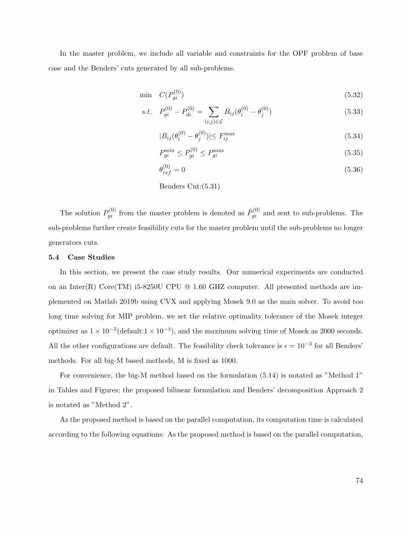
In the master problem, we include all variable and constraints for the OPF problem of base

case and the Benders’ cuts generated by all sub-problems.

min C(P(0)gi ) (5.32)

s.t. P(0)gi − P

(0)di =

∑(i,j)∈L

Bij(θ(0)i − θ

(0)j ) (5.33)

|Bij(θ(0)i − θ(0)j )|≤ Fmax

ij (5.34)

Pmingi ≤ P

(0)gi ≤ P

maxgi (5.35)

θ(0)ref = 0 (5.36)

Benders Cut:(5.31)

The solution P(0)gi from the master problem is denoted as P

(0)gi and sent to sub-problems. The

sub-problems further create feasibility cuts for the master problem until the sub-problems no longer

generators cuts.

5.4 Case Studies

In this section, we present the case study results. Our numerical experiments are conducted

on an Inter(R) Core(TM) i5-8250U CPU @ 1.60 GHZ computer. All presented methods are im-

plemented on Matlab 2019b using CVX and applying Mosek 9.0 as the main solver. To avoid too

long time solving for MIP problem, we set the relative optimality tolerance of the Mosek integer

optimizer as 1× 10−3(default:1× 10−4), and the maximum solving time of Mosek as 2000 seconds.

All the other configurations are default. The feasibility check tolerance is ε = 10−3 for all Benders’

methods. For all big-M based methods, M is fixed as 1000.

For convenience, the big-M method based on the formulation (5.14) is notated as ”Method 1”

in Tables and Figures; the proposed bilinear formulation and Benders’ decomposition Approach 2

is notated as ”Method 2”.

As the proposed method is based on the parallel computation, its computation time is calculated

according to the following equations: As the proposed method is based on the parallel computation,

74

its computation time is calculated according to the following equations:

T =∑i∈l

maxj∈c

(tji )

where, T means the total computation time, c is the set of contingency index, l is the set of iteration

sequence, tji means the time consuming of the jth contingency at the ith iteration.

For an SCOPF problem, some conflicting contingencies may exist. Those contingencies can

not co-exist in the contingencies sets of SCOPF problems [87]. In this chapter, we identified he

removed all conflicting contingencies in the test cases. The identified conflicting contingencies are

list in Table 5.2.

Table 5.2: Conflict contingencies in all cases.

Cases Conflict contingencies

Case3 None

Case5 G3

Case14 None

G31, G32, G33, G34, G35, G36, L1−2

L1−39, L2−30, L4−14, L6−11, L6−31, L10−11

case39 L10−13, L10−32, L13−14, L16−19, L17−18, L19−20

L19−33, L20−34, L21−22, L22−35, L23−36, L25−26

L25−37, L26−27, L29−38

case118 L85−86, L110−111, L68−116, L12−117

5.4.1 Three-bus System

In this subsection, we show that the proposed method (Method 2) is capable of correctly reflect-

ing the generator response based on its post-contingency response constraints (5.13). The testbed

system is a three-bus three-machine system. The topology of the system is presented in Fig. 5.31.

The parameters of the branches and generators are listed in Table 5.3

Table 5.3: 3-bus system parameters.

C2 C1 C0 Pmax Pmin α

G1 0.11 5 150 3000 0 1/30G2 0.085 1.2 100 300 0 1/3G3 0.055 1 50 400 0 19/30

B1,2,3 X = 0.0504(p.u) Fmax = 3(p.u)

In the first experiment, load varying is treated as contingency scenarios. Outage is not consid-

ered. Total 7 contingency scenarios are considered in the SCOPF problem. Fig.5.4 presents the

75

G1 G2

G3

1 2

3

B3

B1

B250MW 170MW

170MW

Figure 5.3: 3 bus system topology

generator post-contingency responses. The x-axis is the load change against the base case load

level. The y-axis notates the variation in generator power against the base case generation. It can

be seen that the response of G2 and G3 comply with the feasible region defined by participation

factor, low and upper bounds. On the other hand, G1 is the reference generator. When either one

of the two generators hit the limit, G1 will no longer assume the designed participation factor of

1/30.

-4 -2 0 2 4 6(k)(p.u)

-2

-1

0

1

2

3

Pg(k

) (p.u

)

Pg1(k) P

g2(k) P

g3(k)

No contingency

(-3.003,-1.001)

(-3.003,-0.1001)

(-3.003,-1.9019)

(3.315,1.105)

(1.17,0.741)

(1.17,0.039)

Figure 5.4: Generators response for load variation. G2 and G3 comply with the feasible regionsdefined by the participation factor, low and upper bounds.

In the second experiment, N-1 contingencies are considered. There are 6 contingencies (3

generator outages, and 3 branch outages). We assume that the reference generator (G1) never fails

in ay scenario, so only 5 contingencies will be considered in this example.

This SCOPF is solved by the proposed method (Method 2) and the off-shelf solver (Mosek) via

big-M formulation (Method 1). Comparison is made on the solution and the computing time. The

76

solution results are listed in Table 5.5. The results show the objective value for two methods are

the same. The computation time of the big-M method is slightly less than the proposed method.

This is due to the small-size of the system. The advantage of the proposed method on computation

efficiency will be demonstrated for larger-scale power grids. This point will be validated using an

118-bus system.

Table 5.4: Comparison of objective values for the Big-M method and the proposed method.

Load Variation N-1 Contingency

Method 1 obj 4946.17 4946.17

Method 2 obj 4946.17 4946.17

Table 5.5 lists the solutions for the second SCOPF problem (the second experiment). In all

branch outage scenarios, the generator power outputs in post-contingency are the same as those in

the base case. In a contingency scenario with G2 outage, the set of the online generators included

G1 and G3. Due to the loss of G2, the change of total is 1.2219 p.u. G1 and G3 now share the

total power generation change according to their participation factors: 1/30 : 19/30 = 5% : 95%.

Hence G1 is expected to share 5% (= 0.8326−0.77151.2219 ) of the total power change, while G3 is expected

to share 95% (= 3.0647−0.77151.2219 ). The solution matches the expected results.

For G3 outage, ∆(k) = 1.9066 p.u. G1 and G2 share the power change according to their

participation factors: 1/30 : 1/3 = 1 : 10. The solution shows that the power increase of G1 is

0.9448 − 0.7715 = 0.1733 and the power increase of G2 is 2.9552 − 1.2219 = 1.7333. Hence, the

generators respond as expected for post contingency.

Table 5.5: Solution for the N-1 contingency SCOPF

Base case Gen 2 outage Gen 3 outage All branch outage

Pg1 0.7715 0.8326 0.9448 0.7715

Pg2 1.2219 − 2.9552 1.2219

Pg3 1.9066 3.0674 − 1.9066

5.4.2 IEEE 118-bus System

Data of the IEEE 118-bus system are from MATPOWER [56]. The line flow limit is set to 500

MVA. In all tests, 100% load means the total load is 42.42 pu. This system consists of 186 branches

and 54 generators. Thus, based on ”N-1” criterion, there could be 240 contingencies. Part of the

77

contingencies are selected for SCOPF. The information of the selected contingencies is listed in

Table 5.6. Eight critical contingencies, identified by [79] and [88], are included in all situations.

The rest are randomly selected.

Table 5.6: 118 bus contingency information.

Number of Number of Number ofselected Branch Generator

contingency contingency contingency

8 4 420 10 1030 15 1540 20 2050 25 25

Critical contingencies

L26−30, L34−37, L38−37, L70−71

G65, G66, G80, G89

Fig. 5.5 presents the lower bound computed by the master problem and maximum of the

solutions from sub-problems associate with contingent scenarios, along with the iteration. It can

be seen that the lower bound converges when all sub-problems become feasible. The tested example

is the 118 bus system with 190% load.

1 2 3 4 5 6 7 82820.6

2820.65

2820.7

2820.75

Low

er b

ound

($)

1 2 3 4 5 6 7 8

Iteraions

0

0.05

0.1

0.15

0.2

Max

imum

infe

asib

ility

(p.

u)

Figure 5.5: Lower bound computed from the master problem converges while an maximum of thesub-problem solutions converges to zero. The test case is the IEEE 118-bus with 190% load.

The computation time of two methods are presented in Figs. 5.6 and 5.7. Fig. 5.6 presents

computing time versus loading level for three SCOPF problems which include 8, 30, 50 contingencies

78

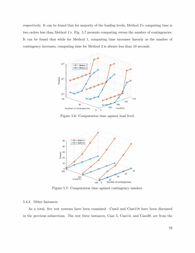
respectively. It can be found that for majority of the loading levels, Method 2’s computing time is

two orders less than Method 1’s. Fig. 5.7 presents computing versus the number of contingencies.

It can be found that while for Method 1, computing time increases linearly as the number of

contingency increases, computing time for Method 2 is always less than 10 seconds.

Figure 5.6: Computation time against load level.

Figure 5.7: Computation time against contingency number.

5.4.3 Other Instances

As a total, five test systems have been examined. Case3 and Case118 have been discussed

in the previous subsections. The rest three instances, Case 5, Case14, and Case39, are from the

79

MATPOWER case library. The total load of Case3 is set as 3.51 p.u. For Case14, line flow limit

100 MW is imposed. For each instance, the participation factors of generators are defined as a set

of fixed positive values with their sum as 1. Table 5.7 presents the information of the three test

cases solved by the two methods. In Table 5.7, the NAN result means that the correspond methods

failed to find reasonable solution within time limit.

For Case3 and Case5, the two methods results the same solution. For Case14, Case39, Case118,

as the problem dimension increases, Method 2 becomes more computing efficient compared to

Method 1. The solution of Case39 is NAN. This means that the big-M formulation and Mosek

solver can not find a reasonable solution within the time limits of 2000 seconds.

Table 5.7: Comparison in different methods

Case # of # of Method Obj Time Iterationcontingencies binary

Case3 5 16Method 1 4128.20 0.14 −Method 2 4128.20 0.55 1

Case5 9 66Method 1 22869.60 1.59 −Method 2 22869.60 2.56 5

Case14 24 184Method 1 8459.71 34.36 −Method 2 8459.71 1.98 3

Case39 27 480Method 1 NAN 2000 −Method 2 41945.24 5.72 5

Case118 235 24804Method 1 130508.80 1143.39 −Method 2 130508.70 3.89 3

5.5 Conclusion

This chapter proposes a bilinear mixed integer programming formulation and an efficient solv-

ing approach for security constrained DCOPF to consider generators’ post-contingency responses.

Through preserving bilinear expressions related to the base case power generation while relaxing

the rest bilinear expressions via McCormick envelops, we designed a Benders’ decomposition strat-

egy that yields to efficient solving. Case study results demonstrate the efficiency of the proposed

formulation compared to the state-of-the-art formulations.

80

Chapter 6: Conclusion and Future Plan

6.1 Conclusion

This dissertation conducted researches about the application of the power system optimization.

It focuses on three major problems: ACOPF, MPC, and SCOPF. For the research about the

ACOPF, we developed an convex relaxation based ACOPF solver which is capable to solve ACOPF

for large size power system. To deal with the exactness issue of the convex relaxation formulation

of ACOPF, two algorithm has been studied. For MPC problem, a Benders’ decomposition based

computational algorithm is implemented on the MMC dynamic model based MPC problem. For

the SCOPF, a new method to solve SCOPF with generator response constraints is investigated.

The benefits of this dissertation research are summarized as follows:

6.1.1 A Sparse Convex ACOPF Solver Based on 3-node Cycles

In the Chapter 2, we proposed a 3-node cycle decomposition based sparse convex relaxation for

ACOPF. We have shown that the 3-node cycle decomposition can not guarantee that the resulting

graph is a chordal graph. However, the proposed relaxation can achieve the close tightness as SDP

OPF solvers. On the other hand, our method has a clearly higher computing efficiency.

6.1.2 Exactness of the Convex Relaxation

In the Chapter 3, an efficient convex iteration implementation is also investigated for the pro-

posed sparse convex solver to achieve exactness or rank-1 solutions. Our experiment results show

the feasibility of the implementation. Moreover, we proposed a nonlinear programming formulation

for ACOPF. This formulation is based on decision variables that align with SOCP/SDP relaxation.

The proposed formulation exploits power network sparsity feature and employs a small set of minor

constrains related to all 3-node cycles as equality constraints to enforce rank-1 constraint, so the

solution is exact. Case study results demonstrate the correctness of this formulation.

81

6.1.3 Benders’ Decomposition for MPC of a Modular Multi-level Converter

In this chapter, a dynamic model of MMC are derived and then formulated to MPC problem. We

separate the original MPC problem to a master problem and a sub-problem for implement Benders’

decomposition to solve the problem. A N = 4 MMC are selected to test proposed algorithm, and

the solutions for different predict horizon are displayed and compared with the solutions by SQP.

According the results, Benders’ decomposition has great performance on solving the low horizon

MPC problem and much better than SQP method. But for longer horizon (T ≥ 10), even it has

presented potential to solve the problem, the algorithm still need more improvement to reduce the

computing cost.

6.1.4 Security Constrained DC OPF Considering Generator Responses

The Chapter 4 proposes a bilinear mixed integer programming formulation and an efficient solv-

ing approach for security constrained DCOPF to consider generators’ post-contingency responses.

Through preserving bilinear expressions related to the base case power generation while relaxing

the rest bilinear expressions via McCormick envelops, we designed a Benders’ decomposition strat-

egy that yields to efficient solving. Case study results demonstrate the efficiency of the proposed

formulation compared to the state-of-the-art formulations.

6.2 Future Work

6.2.1 Security Constrained ACOPF

The new formulation to handle the generator response constraints in preventive DC SCOPF can

be implemented on ACOPF. The Chapter 4 verified the efficiency of the new Benders’ decomposi-

tion based bilinear formulation to solve the generator response integrated preventive DC SCOPF.

Because of the formulation is only related with power, it should be easy to be implemented on the

AC SCOPF. The convex relaxation can be applied to deal with the AC power flow constraints.

6.2.2 OPF in Renewable Energy Source Integrated Power System

In recent years, as the increasing of the renewable energy sources, the uncertainty of the re-

newable energy sources becomes an big challenge for the traditional OPF mechanism. Some new

algorithm, such as the multi-stage stochastic programming, worst case optimization, and chance

constrained optimization are implemented to deal with this issue. However, the complexity of the

82

OPF has been significantly increased, because the new algorithms need to add additional vari-

ables and constraints. Therefore, the method to improve the calculation speed still needs more

investigation.

83

References

[1] M. E. Initiative, “The future of the electric grid,” 2011. [Online]. Available: https://sites.suffolk.edu/mminobe93/2015/09/20/u-s-energy-grid/

[2] R. Bansal, “Optimization methods for electric power systems: An overview,” InternationalJournal of Emerging Electric Power Systems, vol. 2, no. 1, 2005.

[3] L. Li, Convex Relaxation. Berlin, Heidelberg: Springer Berlin Heidelberg, 2015, pp. 115–126.[Online]. Available: https://doi.org/10.1007/978-3-662-46356-7 6

[4] A. Castillo and R. P. O’Neill, “Survey of approaches to solving the acopf (opf paper 4),” USFederal Energy Regulatory Commission, Tech. Rep, 2013.

[5] W. A. Bukhsh, A. Grothey, K. I. McKinnon, and P. A. Trodden, “Local solutions of the optimalpower flow problem,” IEEE Transactions on Power Systems, vol. 28, no. 4, pp. 4780–4788,2013.

[6] S. H. Low, “Convex relaxation of optimal power flow—part i: Formulations and equivalence,”IEEE Transactions on Control of Network Systems, vol. 1, no. 1, pp. 15–27, 2014.

[7] J. BnnoBRs, “Partitioning procedures for solving mixed-variables programming problems ‘,”1962.

[8] R. Rahmaniani, T. G. Crainic, M. Gendreau, and W. Rei, “The benders decomposition algo-rithm: A literature review,” European Journal of Operational Research, vol. 259, no. 3, pp.801–817, 2017.

[9] A. M. Geoffrion and G. W. Graves, “Multicommodity distribution system design by bendersdecomposition,” Management science, vol. 20, no. 5, pp. 822–844, 1974.

[10] J. Carpentier, “Contribution to the economic dispatch problem,” Bulletin de la Societe Fran-coise des Electriciens, vol. 3, no. 8, pp. 431–447, 1962.

[11] D. I. Sun, B. Ashley, B. Brewer, A. Hughes, and W. F. Tinney, “Optimal power flow by newtonapproach,” IEEE Transactions on Power Apparatus and systems, no. 10, pp. 2864–2880, 1984.

[12] G. L. Torres and V. H. Quintana, “An interior-point method for nonlinear optimal power flowusing voltage rectangular coordinates,” IEEE transactions on Power Systems, vol. 13, no. 4,pp. 1211–1218, 1998.

[13] X. Bai, H. Wei, K. Fujisawa, and Y. Wang, “Semidefinite programming for optimal power flowproblems,” International Journal of Electrical Power & Energy Systems, vol. 30, no. 6, pp.383–392, 2008.

84

[14] R. A. Jabr, “Radial distribution load flow using conic programming,” IEEE transactions onpower systems, vol. 21, no. 3, pp. 1458–1459, 2006.

[15] M. B. Cain, R. P. O’neill, and A. Castillo, “History of optimal power flow and formulations,”Federal Energy Regulatory Commission, pp. 1–36, 2012.

[16] J. Lavaei and S. H. Low, “Zero duality gap in optimal power flow problem,” IEEE Transactionson Power Systems, vol. 27, no. 1, pp. 92–107, 2012.

[17] B. Kocuk, S. S. Dey, and X. A. Sun, “Inexactness of sdp relaxation and valid inequalities foroptimal power flow,” IEEE Transactions on Power Systems, vol. 31, no. 1, pp. 642–651, 2016.

[18] B. C. Lesieutre, D. K. Molzahn, A. R. Borden, and C. L. DeMarco, “Examining the limitsof the application of semidefinite programming to power flow problems,” in Communication,Control, and Computing (Allerton), 2011 49th Annual Allerton Conference on. IEEE, 2011,pp. 1492–1499.

[19] R. Madani, M. Ashraphijuo, and J. Lavaei, “Promises of conic relaxation for contingency-constrained optimal power flow problem,” IEEE Transactions on Power Systems, vol. 31,no. 2, pp. 1297–1307, 2016.

[20] D. K. Molzahn, C. Josz, I. A. Hiskens, and P. Panciatici, “A laplacian-based approach for find-ing near globally optimal solutions to opf problems,” IEEE Transactions on Power Systems,vol. 32, no. 1, pp. 305–315, 2017.

[21] S. You and Q. Peng, “A non-convex alternating direction method of multipliers heuristic foroptimal power flow,” in Smart Grid Communications (SmartGridComm), 2014 IEEE Inter-national Conference on. IEEE, 2014, pp. 788–793.

[22] B. Kocuk, S. S. Dey, and X. A. Sun, “Matrix minor reformulation and socp-basedspatial branch-and-cut method for the ac optimal power flow problem,” arXiv preprintarXiv:1703.03050, 2017.

[23] W. Wang and N. Yu, “Chordal conversion based convex iteration algorithm for three-phaseoptimal power flow problems,” IEEE Transactions on Power Systems, 2017.

[24] W. Wei, J. Wang, N. Li, and S. Mei, “Optimal power flow of radial networks and its variations:A sequential convex optimization approach,” IEEE Transactions on Smart Grid, vol. 8, no. 6,pp. 2974–2987, 2017.

[25] P. Cortes, M. P. Kazmierkowski, R. M. Kennel, D. E. Quevedo, and J. Rodriguez, “Predictivecontrol in power electronics and drives,” IEEE Transactions on Industrial Electronics, vol. 55,no. 12, pp. 4312–4324, Dec 2008.

[26] Y. Ma, L. Fan, and Z. Miao, “Realizing space vector modulation in matlab/simulink andpscad,” in 2013 North American Power Symposium (NAPS). IEEE, 2013, pp. 1–6.

[27] S. Kouro, P. Cortes, R. Vargas, U. Ammann, and J. Rodrıguez, “Model predictive control—asimple and powerful method to control power converters,” IEEE Transactions on industrialelectronics, vol. 56, no. 6, pp. 1826–1838, 2008.

85

[28] L. Platbrood, F. Capitanescu, C. Merckx, H. Crisciu, and L. Wehenkel, “A generic approachfor solving nonlinear-discrete security-constrained optimal power flow problems in large-scalesystems,” IEEE Transactions on Power Systems, vol. 29, no. 3, pp. 1194–1203, 2014.

[29] A. Monticelli, M. Pereira, and S. Granville, “Security-constrained optimal power flow withpost-contingency corrective rescheduling,” IEEE Transactions on Power Systems, vol. 2, no. 1,pp. 175–180, 1987.

[30] B. Stott and O. Alsac, “Optimal power flow: Basic requirements for real-life problems andtheir solutions,” in SEPOPE XII Symposium, Rio de Janeiro, Brazil, vol. 11, 2012.

[31] D. Phan and J. Kalagnanam, “Some efficient optimization methods for solving the security-constrained optimal power flow problem,” IEEE Transactions on Power Systems, vol. 29, no. 2,pp. 863–872, 2013.

[32] T. Sennewald, F. Sass, and D. Westermann, “A preventive security constrained optimal powerflow for mixed ac-hvdc-systems,” 2017.

[33] F. Capitanescu, M. Glavic, D. Ernst, and L. Wehenkel, “Applications of security-constrainedoptimal power flows,” in In Proceedings of Modern Electric Power Systems Symposium,MEPS06, 2006.

[34] V. Hinojosa and F. Gonzalez-Longatt, “Preventive security-constrained dcopf formulation us-ing power transmission distribution factors and line outage distribution factors,” Energies,vol. 11, no. 6, p. 1497, 2018.

[35] K. Sundar, H. Nagarajan, L. Roald, S. Misra, R. Bent, and D. Bienstock, “Chance-constrainedunit commitment with n-1 security and wind uncertainty,” IEEE Transactions on Control ofNetwork Systems, 2019.

[36] M. Velay, M. Vinyals, Y. Besanger, and N. Retiere, “Fully distributed security constrainedoptimal power flow with primary frequency control,” International Journal of Electrical Power& Energy Systems, vol. 110, pp. 536–547, 2019.

[37] M. Carrion, Y. Dvorkin, and H. Pandzic, “Primary frequency response in capacity expansionwith energy storage,” IEEE Transactions on Power Systems, vol. 33, no. 2, pp. 1824–1835,2017.

[38] Y. Dvorkin, P. Henneaux, D. S. Kirschen, and H. Pandzic, “Optimizing primary response inpreventive security-constrained optimal power flow,” IEEE Systems Journal, vol. 12, no. 1,pp. 414–423, 2016.

[39] M. Ma, L. Fan, Z. Miao, B. Zeng, and H. Ghassempour, “A sparse convex ac opf solver andconvex iteration implementation based on 3-node cycles,” Electric Power Systems Research,vol. 180, p. 106169, 2020.

[40] H. W. Dommel and W. F. Tinney, “Optimal power flow solutions,” IEEE Transactions onpower apparatus and systems, no. 10, pp. 1866–1876, 1968.

86

[41] F. Milano, C. A. Canizares, and A. J. Conejo, “Sensitivity-based security-constrained opfmarket clearing model,” IEEE Transactions on power systems, vol. 20, no. 4, pp. 2051–2060,2005.

[42] R. Zarate-Minano, F. Milano, and A. J. Conejo, “An opf methodology to ensure small-signalstability,” IEEE Transactions on Power Systems, vol. 26, no. 3, pp. 1050–1061, 2011.

[43] S. H. Low, “Convex relaxation of optimal power flow—part ii: Exactness,” IEEE Transactionson Control of Network Systems, vol. 1, no. 2, pp. 177–189, 2014.

[44] ——, “Convex relaxation of optimal power flow part i: Formulations and equivalence,” IEEETransactions on Control of Network Systems, vol. 1, no. 1, pp. 15–27, 2014.

[45] R. A. Jabr, “Exploiting sparsity in SDP relaxations of the OPF problem,” IEEE Transactionson Power Systems, vol. 27, no. 2, pp. 1138–1139, 2012.

[46] D. K. Molzahn, J. T. Holzer, B. C. Lesieutre, and C. L. DeMarco, “Implementation of a large-scale optimal power flow solver based on semidefinite programming,” IEEE Transactions onPower Systems, vol. 28, no. 4, pp. 3987–3998, 2013.

[47] M. Fukuda, M. Kojima, K. Murota, and K. Nakata, “Exploiting sparsity in semidefinite pro-gramming via matrix completion i: General framework,” SIAM Journal on Optimization,vol. 11, no. 3, pp. 647–674, 2001.

[48] R. Madani, M. Ashraphijuo, and J. Lavaei. (2014) SDP Solver of Optimal Power Flow User’sManual. [Online]. Available: http://ieor.berkeley.edu/∼lavaei/Software.html

[49] B. Kocuk, S. S. Dey, and X. A. Sun, “Strong socp relaxations for the optimal power flowproblem,” Operations Research, vol. 64, no. 6, pp. 1177–1196, 2016.

[50] Z. Miao, L. Fan, H. G. Aghamolki, and B. Zeng, “Least Squares Estimation Based SDP Cutsfor SOCP Relaxation of AC OPF,” IEEE Transactions on Automatic Control, vol. 63, no. 1,pp. 241–248, Jan 2018.

[51] C. Bingane, M. F. Anjos, and S. Le Digabel, “Tight-and-cheap conic relaxation for the acoptimal power flow problem,” IEEE Transactions on Power Systems, vol. 33, no. 6, pp. 7181–7188, 2018.

[52] H. Johnston, “Cliques of a graph-variations on the Bron-Kerbosch algorithm,” InternationalJournal of Parallel Programming, vol. 5, no. 3, pp. 209–238, 1976.

[53] J. Wildman, “Bron-Kerbosch maximal clique finding algorithm,” https://www.mathworks.com/matlabcentral/fileexchange/30413-bron-kerbosch-maximal-clique-finding-algorithm,2011.

[54] K. Mehlhorn and D. Michail, “Implementing minimum cycle basis algorithms,” Journal ofExperimental Algorithmics (JEA), vol. 11, pp. 2–5, 2007.

[55] S. Iglin, “grTheory - Graph Theory Toolbox,” https://www.mathworks.com/matlabcentral/fileexchange/4266-grtheory-graph-theory-toolbox?focused=5177310&tab=function, 2011.

87

[56] R. D. Zimmerman, C. E. Murillo-Sanchez, and R. J. Thomas, “Matpower: Steady-state oper-ations, planning, and analysis tools for power systems research and education,” IEEE Trans-actions on power systems, vol. 26, no. 1, pp. 12–19, 2011.

[57] C. Coffrin, D. Gordon, and P. Scott. (2014) NESTA, the NICTA energy system test casearchive. [Online]. Available: http://arxiv.org/abs/1411.0359

[58] M. Grant, S. Boyd, and Y. Ye, “CVX: Matlab software for disciplined convex programming,”2008.

[59] M. Ma and L. Fan, “Rank-1 positive semidefinite matrix-based nonlinear programming formu-lation for ac opf,” International Transactions on Electrical Energy Systems, vol. 29, no. 10, p.e12095, 2019.

[60] C. Chen, A. Atamturk, and S. S. Oren, “A spatial branch-and-cut method for nonconvex qcqpwith bounded complex variables,” Mathematical Programming, vol. 165, no. 2, pp. 549–577,2017.

[61] W. Wang and N. Yu, “Chordal conversion based convex iteration algorithm for three-phaseoptimal power flow problems,” IEEE Transactions on Power Systems, vol. 33, no. 2, pp.1603–1613, 2018.

[62] Y. Shi, H. Tuan, P. Apkarian, and A. Savkin, “Global optimal power flow over large-scalepower transmission networks,” Systems & Control Letters, vol. 118, pp. 16–21, 2018.

[63] S. Bose, S. H. Low, T. Teeraratkul, and B. Hassibi, “Equivalent relaxations of optimal powerflow,” IEEE Transactions on Automatic Control, vol. 60, no. 3, pp. 729–742, 2015.

[64] J. Dattorro, Convex optimization & Euclidean distance geometry. Lulu. com, 2010.

[65] M. Ma, L. Fan, Z. Miao, B. Zeng, and H. Ghassempour, “Strengthened socp relaxation forac opf and rank-1 computing based on 3 -node cycles,” under review, IEEE Transactions onPower Systems, 2018.

[66] M. Grant, S. Boyd, and Y. Ye, “Cvx: Matlab software for disciplined convex programming,”2008.

[67] M. Ma and L. Fan, “Bender’s decomposition algorithm for model predictive control of a mod-ular multi-level converter,” in 2017 North American Power Symposium (NAPS). IEEE, 2017,pp. 1–6.

[68] L. Franquelo, J. Rodriguez, J. Leon, S. Kouro, R. Portillo, and M. Prats, “The age of multilevelconverters arrives,” Industrial Electronics Magazine, IEEE, vol. 2, no. 2, pp. 28–39, June 2008.

[69] M. Saeedifard and R. Iravani, “Dynamic performance of a modular multilevel back-to-backhvdc system,” Power Delivery, IEEE Transactions on, vol. 25, no. 4, pp. 2903–2912, Oct2010.

[70] M. Hiller, D. Krug, R. Sommer, and S. Rohner, “A new highly modular medium voltageconverter topology for industrial drive applications,” in Power Electronics and Applications,2009. EPE ’09. 13th European Conference on, Sept 2009, pp. 1–10.

88

[71] M. Winkelnkemper, A. Korn, and P. Steimer, “A modular direct converter for transformerlessrail interties,” in Industrial Electronics (ISIE), 2010 IEEE International Symposium on, July2010, pp. 562–567.

[72] B. Li, R. Yang, D. Xu, G. Wang, W. Wang, and D. Xu, “Analysis of the phase-shifted carriermodulation for modular multilevel converters,” Power Electronics, IEEE Transactions on,vol. 30, no. 1, pp. 297–310, Jan 2015.

[73] W. Rei, J.-F. Cordeau, M. Gendreau, and P. Soriano, “Accelerating benders decompositionby local branching,” INFORMS Journal on Computing, vol. 21, no. 2, pp. 333–345, 2009.

[74] T. L. Magnanti and R. T. Wong, “Accelerating benders decomposition: Algorithmic enhance-ment and model selection criteria,” Operations research, vol. 29, no. 3, pp. 464–484, 1981.

[75] G. K. Saharidis, M. Minoux, and M. G. Ierapetritou, “Accelerating benders method usingcovering cut bundle generation,” International Transactions in Operational Research, vol. 17,no. 2, pp. 221–237, 2010.

[76] M. Ma and L. Fan, “Security constrained dc opf considering generator responses,” ElectricPower Systems Research, p. 106920, 2020.

[77] O. Alsac and B. Stott, “Optimal load flow with steady-state security,” IEEE transactions onpower apparatus and systems, no. 3, pp. 745–751, 1974.

[78] Y. Yang and Y. Feng, “Large-scale preventive security constrained optimal power flow basedon compensation method,” in 2015 IEEE Power & Energy Society General Meeting. IEEE,2015, pp. 1–5.

[79] Y. Xu, Z. Y. Dong, R. Zhang, K. P. Wong, and M. Lai, “Solving preventive-corrective scopfby a hybrid computational strategy,” IEEE Transactions on Power Systems, vol. 29, no. 3,pp. 1345–1355, 2013.

[80] Y. Wen and C. Guo, “Discussion on “solving preventive-corrective scopf by a hybrid com-putational strategy”,” IEEE Transactions on Power Systems, vol. 29, no. 6, pp. 3124–3124,2014.

[81] L. Yang, C. Zhang, and J. Jian, “A parallel method for solving the dc security constrainedoptimal power flow with demand uncertainties,” International Journal of Electrical Power &Energy Systems, vol. 102, pp. 171–178, 2018.

[82] G. O. Competition. (2018) SCOPF Problem Formulation: Challenge 1. [Online]. Avail-able: https://gocompetition.energy.gov/sites/default/files/SCOPF Formulation GO Comp20181114.pdf

[83] B. Zeng, Y. An, and L. Kuznia, “Chance constrained mixed integer program: Bilinear andlinear formulations, and benders decomposition,” arXiv preprint arXiv:1403.7875, 2014.

[84] Y. Zhang, J. Wang, B. Zeng, and Z. Hu, “Chance-constrained two-stage unit commitmentunder uncertain load and wind power output using bilinear benders decomposition,” IEEETransactions on Power Systems, vol. 32, no. 5, pp. 3637–3647, 2017.

89

[85] H. Haghighat and B. Zeng, “Stochastic and chance-constrained conic distribution system ex-pansion planning using bilinear benders decomposition,” IEEE Transactions on Power Sys-tems, vol. 33, no. 3, pp. 2696–2705, 2017.

[86] Y. Wen, C. Guo, H. Pandzic, and D. S. Kirschen, “Enhanced security-constrained unit com-mitment with emerging utility-scale energy storage,” IEEE Transactions on power Systems,vol. 31, no. 1, pp. 652–662, 2015.

[87] Q. Jiang and K. Xu, “A novel iterative contingency filtering approach to corrective security-constrained optimal power flow,” IEEE Transactions on Power Systems, vol. 29, no. 3, pp.1099–1109, 2013.

[88] F. Karbalaei, H. Shahbazi, and M. Mahdavi, “A new method for solving preventive security-constrained optimal power flow based on linear network compression,” International Journalof Electrical Power & Energy Systems, vol. 96, pp. 23–29, 2018.

90

Appendix A: Copyright Permissions

The permission below is for the Fig. 1.1.

91

The permission below is for the main contents and results of Chapter 2 and Chapter 3.

92

The permission below is for the main contents and results of Chapter 3.

93

94

The permission below is for the main contents and results of Chapter 4.

95

The permission below is for the main contents and results of Chapter 5.

96

About the Author

Minyue (Matthew) Ma, a Ph.D. majoring in Electrical Engineer at the University of South

Florida. He was an intern-engineer at the National Renewable Energy Laboratory, where he assisted

the NREL-MIDAS solar team to develop a renewable energy simulation software. Dr. Ma’s research

interests include power system analysis, modeling, optimization. He has had articles published in

several peer-reviewed journals. He has also presented his works at international, national, and

regional conferences. He received his Master’s degree in Electrical Engineer from the University of

South Florida, and his Bachelor’s degree in Electrical Engineering from the Huazhong University

of Science and Technology in China.