Power Management and Design Optimization of Fuel … optimization of FCHVs in the literature focused...
30
Journal of Power Sources, Vol.165, issue 2, March 2007, pp.819-832. 1 Abstract— Power management strategy is as significant as component sizing in achieving optimal fuel economy of a fuel cell hybrid vehicle (FCHV). We have formulated a combined power management/design optimization problem for the performance optimization of FCHVs. This includes subsystem-scaling models to predict the characteristics of components of different sizes. In addition, we designed a parameterizable and near-optimal controller for power management optimization. This controller, which is inspired by our Stochastic Dynamic Programming results, can be included as design variables in system optimization problems. Simulation results demonstrate that combined optimization can efficiently provide excellent fuel economy. 1. Introduction Power management strategy and component sizing affect vehicle performance and fuel economy considerably in hybrid vehicles because of the multiple power sources and differences in their characteristics. Furthermore, these two important factors are coupled—different design of component sizing should come with different design of power management strategy. Therefore, to achieve maximum fuel economy for hybrid vehicles, optimal power management and component sizing should be determined as a combined package. Our research has formulated and solved a combined power management/design (i.e., control/plant) optimization problem of a fuel cell hybrid vehicle (FCHV). Development of the power management strategy is one of the important tasks in developing hybrid vehicles and relatively many literatures can be found. Guezennec et al. [1] solved the supervisory control problem of a FCHV as a quasi-static optimization problem and found that hybridization can significantly improve the fuel economy of FCHVs. Rodatz et al. [2] used the equivalent consumption minimization strategy 1 Doctoral Candidate, Department of Mechanical Engineering, University of Michigan, Ann Arbor, MI 48109-2125 (734-936-0352, [email protected] ) 2 Professor, Department of Mechanical Engineering, University of Michigan, Ann Arbor, MI 48109-2125 (734-936-0352) Min-Joong Kim 1 and Huei Peng 2 Power Management and Design Optimization of Fuel Cell/Battery Hybrid Vehicles
-
Upload
dangkhuong -
Category
Documents
-
view
214 -
download
0
Transcript of Power Management and Design Optimization of Fuel … optimization of FCHVs in the literature focused...

Journal of Power Sources, Vol.165, issue 2, March 2007, pp.819-832.
1
Abstract— Power management strategy is as significant as component sizing in achieving optimal fuel economy of a
fuel cell hybrid vehicle (FCHV). We have formulated a combined power management/design optimization problem
for the performance optimization of FCHVs. This includes subsystem-scaling models to predict the characteristics
of components of different sizes. In addition, we designed a parameterizable and near-optimal controller for power
management optimization. This controller, which is inspired by our Stochastic Dynamic Programming results, can
be included as design variables in system optimization problems. Simulation results demonstrate that combined
optimization can efficiently provide excellent fuel economy.
1. Introduction
Power management strategy and component sizing affect vehicle performance and fuel economy
considerably in hybrid vehicles because of the multiple power sources and differences in their characteristics.
Furthermore, these two important factors are coupled—different design of component sizing should come with
different design of power management strategy. Therefore, to achieve maximum fuel economy for hybrid
vehicles, optimal power management and component sizing should be determined as a combined package. Our
research has formulated and solved a combined power management/design (i.e., control/plant) optimization
problem of a fuel cell hybrid vehicle (FCHV).
Development of the power management strategy is one of the important tasks in developing hybrid
vehicles and relatively many literatures can be found. Guezennec et al. [1] solved the supervisory control
problem of a FCHV as a quasi-static optimization problem and found that hybridization can significantly
improve the fuel economy of FCHVs. Rodatz et al. [2] used the equivalent consumption minimization strategy
1 Doctoral Candidate, Department of Mechanical Engineering, University of Michigan, Ann Arbor, MI 48109-2125 (734-936-0352,
[email protected]) 2 Professor, Department of Mechanical Engineering, University of Michigan, Ann Arbor, MI 48109-2125 (734-936-0352)
Min-Joong Kim1 and Huei Peng2
Power Management and Design Optimization of Fuel Cell/Battery Hybrid Vehicles

Journal of Power Sources, Vol.165, issue 2, March 2007, pp.819-832.
2
to determine an optimal power distribution for a fuel cell/supercapacitor hybrid vehicle. The concept of
equivalent factors in hybrid electric vehicles has been described by Sciarretta et al. [3]. In the same research,
they also compared their power management result to deterministic dynamic programming result, which can
lead to a global optimality.
Combined optimization problem of power management and component sizing of hybrid vehicles is
analogous to a combined control/plant optimization problem in control theory. Fathy et al. [4] classified
strategies for combined plant/controller optimization into sequential, iterative, bi-level, and simultaneous
strategies. If a plant is optimized first and a controller is then designed, it often leads to non-optimal overall
system due to the coupling of plant/controller optimization. Developing scalable subsystem models is essential
in this optimization problem. Assanis et al. [5] proposed a design optimization framework to find the best
overall engine size, battery pack, and motor combination in maximizing the fuel economy. For the engine
scaling, in particular, they replaced the linear scaling of experimental engine look-up tables with a high-fidelity
simulation that predicts the nonlinear effects of scaling. Fellini et al. [6] presented an optimization algorithm of
this problem. Their research provides a good framework for component sizing, but the control optimization was
not addressed. Design optimization of FCHVs in the literature focused mostly on the relative size between
battery and fuel cell (sometimes referred as the degree of hybridization). Ishikawa et al. of Toyota Motor
Coporation [7] studied the effect of size ratios using their FCHV, but did not explain their control strategy and
optimization procedure. Atwood et al. [8] used ADVISOR, developed by NREL, to study the degree of
hybridization of a FCHV. They changed the ratio of the fuel cell over a fixed total power of powertrain and
checked how the fuel efficiency varied. In a following paper [9], they included control variables in their
optimization problem formulation. This was one of the earliest publications dealing with sequential
control/plant optimization problem of FCHVs despite that the controller could not guarantee optimality.
Another reference was published from Argonne National Laboratory [10], with an approach similar to [9]. In
addition to component sizing optimization, Markel et al. [11] summarized design issues such as cost and
volume in choosing types and sizes of the energy storage system for FCHVs.
Research in the optimization of hybrid vehicles was predominately conducted independently for either
component sizing or control strategy; in rare cases when the two were considered together, control strategies

Journal of Power Sources, Vol.165, issue 2, March 2007, pp.819-832.
3
were largely based on heuristic rules. This made it impossible to achieve true optimization. This study presents
a combined power management/design optimization of FCHVs. The power management algorithm was
developed from Stochastic Dynamic Programming motivated basis functions. In other words, while the control
is not truly optimal, it is optimal in its sub-class. The overall problem is then recast into an optimal parameter
problem.
2. Fuel Cell Vehicle Model and Optimal Power Management Strategy
To study the combined power management/design optimization problem, we used the fuel cell hybrid
vehicle simulation model (FC-VESIM), which was constructed based on the test data of a DaimlerChrysler
prototype fuel cell vehicle Natrium [12]. The powertrain of Natrium consists of an 82 kW peak electric drive
system, a 40 kW Li-ion battery pack and a 75 kW fuel cell engine. The prototype vehicle was tested in various
conditions to verify its performances in highway driving, city driving, rapid acceleration, and maximum travel
range while experimental data are collected from the vehicle components. During the several tests on proving
ground, more than 200 channels of data were collected and used to build the simulation model. In addition to
the vehicle, a fuel cell hybrid powertrain test bench was built. Each subsystem was tested on the bench to obtain
necessary data to build its dynamic model and efficiency map.
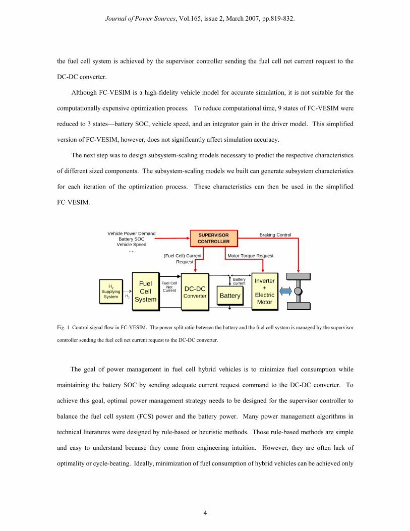
Fig. 1 shows the powertrain schematic of FC-VESIM and key control signals for power management.
FC-VESIM consists of several subsystems: driver, fuel cell system, battery, DC-DC converter, electric drive,
and vehicle dynamics. Considering various vehicle states—such as power demand, battery state of charge
(SOC), and vehicle speed— the supervisor controller sends the fuel cell current request to the DC-DC
converter; sends the motor torque request to the electric drive; and controls the regenerative braking ratio. In
order to generate the motor torque requested from the supervisor controller, the inverter draws current from the
electric DC bus where the battery and the DC-DC converter are connected in parallel. The DC-DC converter
can control the current flow into the DC bus, whereas the battery here is “passively” connected to the DC
bus—the difference between the current draw from the inverter and the current outflow from the DC-DC
converter will be compensated by the passive battery. Therefore, the power split ratio between the battery and
Journal of Power Sources, Vol.165, issue 2, March 2007, pp.819-832.
4
the fuel cell system is achieved by the supervisor controller sending the fuel cell net current request to the
DC-DC converter.
Although FC-VESIM is a high-fidelity vehicle model for accurate simulation, it is not suitable for the
computationally expensive optimization process. To reduce computational time, 9 states of FC-VESIM were
reduced to 3 states—battery SOC, vehicle speed, and an integrator gain in the driver model. This simplified
version of FC-VESIM, however, does not significantly affect simulation accuracy.
The next step was to design subsystem-scaling models necessary to predict the respective characteristics
of different sized components. The subsystem-scaling models we built can generate subsystem characteristics
for each iteration of the optimization process. These characteristics can then be used in the simplified
FC-VESIM.
Batterycurrent
(Fuel Cell) Current Request
SUPERVISOR CONTROLLERSUPERVISOR CONTROLLER
Vehicle Power DemandBattery SOC
Vehicle Speed….
Motor Torque Request
Fuel CellNet
Current DC-DCConverterDC-DCConverter BatteryBattery
Inverter+
ElectricMotor
Inverter+
ElectricMotor
FuelCell
System
FuelCell
System
H2SupplyingSystem
H2SupplyingSystem H2
Braking Control
Fig. 1 Control signal flow in FC-VESIM. The power split ratio between the battery and the fuel cell system is managed by the supervisor
controller sending the fuel cell net current request to the DC-DC converter.
The goal of power management in fuel cell hybrid vehicles is to minimize fuel consumption while
maintaining the battery SOC by sending adequate current request command to the DC-DC converter. To
achieve this goal, optimal power management strategy needs to be designed for the supervisor controller to
balance the fuel cell system (FCS) power and the battery power. Many power management algorithms in
technical literatures were designed by rule-based or heuristic methods. Those rule-based methods are simple
and easy to understand because they come from engineering intuition. However, they are often lack of
optimality or cycle-beating. Ideally, minimization of fuel consumption of hybrid vehicles can be achieved only

Journal of Power Sources, Vol.165, issue 2, March 2007, pp.819-832.
5
when the driving scenario is known a priori. The deterministic dynamic programming technique can
accomplish this global optimum. Then again, the result cannot be realized as a power management scheme
because it is not possible to predict the future driving scenario.
The power management strategy designed by the stochastic dynamic programming (SDP) approach can
overcome these limitations of existing algorithms [12]. The idea of the infinite horizon SDP is that if the
overall power demand is modeled as a stochastic process, an optimal controller can be designed based on the
stochastic model. First, the driver power demand is modeled as a discrete-time stochastic dynamic process by
using a Markov chain model, which is constructed from standard driving cycles. In other words, the power
demand from the drive at the next time step depends on the current power demand and vehicle speed:
{ }, Pr ,
for , 1, 2,..., , 1,2,...,
j i lil j dem dem dem wh wh
p
p w P P P
i j N l Nω
ω ω= = = =
= = (1)
where the power demand demP and the wheel speed whω are quantized into grids of pN and Nω respectively.
Then, for the discretized state vector, ( , , )wh demx SOC Pω= , corresponding optimal fuel cell current request
command, , ,fc net requ I= , is determined to minimize the expected cost of hydrogen consumption and battery
energy usage over infinite horizon:
( )2
1
,0
limk
Nk
H rct socN w kJ E W Wγ
−
→∞=
⎧ ⎫= +⎨ ⎬
⎩ ⎭∑ (2)
where 0< γ <1 is the discount factor, 2 ,H rctW is the reacted hydrogen mass, and Wsoc penalizes the battery energy
use based on the SOC value. This SDP problem can be either solved by a policy iteration or value iteration
process. The resulting SDP control strategy generates optimal fuel cell current request as a function of battery
SOC, wheel speed, and power demand. The control strategy achieves high fuel economy while successfully
maintaining battery SOC.
Despite the advantages of the SDP approach, it is computationally expensive to build tables and get a
corresponding optimal control for complex dynamic systems. Moreover, component design variables cannot
be included in a standard SDP problem formulation. The iterative algorithms solving SDP problems need a cost
table and a transition probability table, but those tables can be constructed only by a vehicle model with fixed

Journal of Power Sources, Vol.165, issue 2, March 2007, pp.819-832.
6
component sizes—if we want to change component sizes in optimization process, we end up getting double
loop of time consuming iteration process (Fig. 2). This makes iterations for different system designs even more
difficult. These limitations of the SDP approach, therefore, make it unsuitable for combined power
management/design optimization problems.
To overcome these limitations of the SDP approach, we developed a near-optimal controller for
optimization process. This controller has an advantage over the SDP—it can be included as several design
variables in the standard optimization process because it is parameterized. On the other hand, because of its
similarity to the SDP result, the controller has advantage over heuristic methods in that it is near-optimal.
Satisfy operating
constraints?
Satisfy operating
constraints?
Get optimal control/plantGet optimal control/plant
YES
NO
Meet optimizationconvergence criteria?
Meet optimizationconvergence criteria?
Changeplant variables/ cost function
Changeplant variables/ cost function
NO
YES
Initialize parametersand variables
Initialize parametersand variables
Build Markov chain modelBuild Markov chain model
Build cost tableBuild cost table
Solve optimal controlSolve optimal control
Run simulationRun simulation
Modifycost function
Modifycost function
PowerManagementOptimization
Power Management/DesignOptimization
ComputationallyExpensive Steps
Fig. 2 Flowchart of combined power management/design optimization problem if SDP process is applied. Double loops of
computationally expensive steps in the SDP make this process infeasible.
3. Methods
This Section describes how the combined power management/design optimization problem was
formulated. Section 3.1 explains how the fuel cell system and the battery are scaled, and how the concept of
degree of hybridization places restriction on the amount of active materials in fuel cells and battery. In Section
3.2, the optimal controller result based on the stochastic dynamic programming is parameterized, so that the

Journal of Power Sources, Vol.165, issue 2, March 2007, pp.819-832.
7
power management strategy can be included as design variables in the optimization process. The final form of
problem statement is made in Section 3.3.
3.1. Subsystem-scaling Models of Fuel Cell Hybrid Powertrain
Although linear scaling is appropriate for predicting system characteristics when size deviations from
the baseline design are small, it becomes less accurate when the deviations are large, especially for highly
nonlinear systems. Therefore, we found it necessary to develop subsystem scaling models for fuel cell hybrid
powertrains that could predict the sizing effects of components including the number of fuel cells, compressor
diameter and battery capacity.
3.1.1. Fuel Cell System Scaling Model
We developed a static FCS scaling model to predict how the design variables—number of fuel cells and
compressor diameter scale—affect the efficiency characteristics of the fuel cell system. The fuel cell system
consists of the fuel cell stack, which is a serially layered pack of fuel cells, and the system auxiliary components,
which include compressor, cooling/heating devices, and water management systems. For the fuel cell stack,
because change in the active cell area requires the complete redesign of flow channels, we chose the number of
fuel cells as a design variable. Among the auxiliary components, we chose the compressor diameter scale as a
design variable because the compressor power is the biggest draw on fuel cell auxiliary powers.
Since the fuel cell system is the primary power source of fuel cell hybrid vehicles, the fuel cell stack is
the core of the powertrain—it is comparable to the cylinders of the combustion engine. Possible design changes
of the fuel cell stack are the number of fuel cells and the active cell area. By changing them, we can obtain
different characteristics of the fuel cell stack current and voltage relation. To build the current-voltage relation
model, we collected data from the fuel cell system on a test bench [12], did the curve-fitting, and obtained the
polarization curve, which is shown in Fig. 3. Here, we assumed that the temperature is maintained at the
operating condition (around 75~80°C) and ignored the effect of the pressure difference between the cathode
and the anode. As a result, the cell voltage (Vcell) is denoted by the current density (ist) and the system pressure
(psys): Vcell = f (ist, psys). We used this equation as the reference of fuel cell stack scaling because the polarization
curve is the property of the fuel cell, which remains unaffected by the fuel cell stack design. Theoretically, if

Journal of Power Sources, Vol.165, issue 2, March 2007, pp.819-832.
8
the number of fuel cells is changed, the y-axis of the polarization curve is scaled because the cells are serially
connected. It is easy to change the number of fuel cells because fuel cell units can be easily stacked. On the
other hand, if the fuel cell active area is changed, we should get the x-axis scaled because the unit of the x-axis
is the current density (A/cm2). However, in practice, it is not simple to modify the active cell area because it
requires re-design of the reactant flow channel, which is a complicated and time-consuming process. Moreover,
the re-design of the reactant flow channel can influence the humidity and thermal characteristics of the stack,
and consequently it may not be guaranteed that the same polarization curve can be used for the scaled design.
Therefore, for practical design purpose, only the number of fuel cells (nfc) is chosen as a design variable for the
fuel cell stack in this study.
0.55
0.6
0.65
0.7
0.75
0.8
0.85
0.9
0.95
1
Current Density [A/cm2]
Cel
l Vol
tage
[V
]
0 0.1 0.2 0.3 0.4 0.5 0.6 0.7
0.45
0.5
0.55
0.6
0.65
0.7
0.75
0.8Fuel Cell Polarization Curves / Pressure Effects
Cel
l Effic
ienc
y
Fig. 3 Fuel cell polarization curve with respect to different levels of cathode pressure. Changes in the fuel cell stack design do not affect this
curve since it is the property of the cell.
Among the fuel cell auxiliary components, the compressor draws our most attention in terms of system
efficiency, because the compressor is the most energy-consuming component. From our data shown in Fig. 4,
the compressor power can be up to 30% of the fuel cell system stack power, whereas power consumption by
other auxiliary components is relatively not as significant as that of the compressor. Similar observation was
reported by Boettner et al. [13], where the compressor power is up to 93.5% of the total auxiliary power
consumption. Therefore, we chose the compressor diameter scale as a design variable because the compressor

Journal of Power Sources, Vol.165, issue 2, March 2007, pp.819-832.
9
is the major draw on auxiliary power, whereas power consumptions of other auxiliaries are linearly scaled by
the number of fuel cells.
0 50 100 150 200 250 3000
10
20
30
40
50
60
70
80
FC stack current [A]
Pow
er [K
W]
FC stack power
FC net powerCompressor power
Other auxiliary power
Fig. 4 Comparison of fuel cell stack power, net power, and auxiliary power versus fuel cell stack current. The compressor auxiliary power
is most influential determining the fuel cell net power and fuel cell system efficiency because it dominates the fuel cell auxiliary power.
We developed a static FCS model based on the model parameters of our test data and previous study
[14]. To reduce the computational time of the optimization process, the FCS scaling model eventually will
build simple static maps, which relate the fuel cell net current to the fuel cell stack voltage, auxiliary power, and
hydrogen fuel consumption. The static FCS scaling model takes the stack current as the system input. Since the
stack current determines the amount of reacted oxygen, we can calculate the required amount of air inflow to
the cathode by assuming constant excess ratio and mass fraction of the oxygen. In reality, before we draw net
current from the fuel cell system and the internal controller starts to drive the compressor motor, we cannot
estimate the fuel cell stack current in advance. However, since there is no dynamics involved in this scaling
model, causality is not an issue because all the input-output relations are stationary one-to-one
correspondences.

Journal of Power Sources, Vol.165, issue 2, March 2007, pp.819-832.
10
Fig. 5 Air supplying subsystem of fuel cell system. Static compressor model determines the amount of the air supply by the compressor
from the amount of oxygen reacted in the fuel cell cathode.
Fig. 5 illustrates the air supplying system for the fuel cell cathode. No sizing issue is involved in the
anode side because a pressurized tank and a control valve are typically used to supply hydrogen fuel. In this
scaling model, therefore, only the air supplying subsystem will be considered. For a given stack current level,
the inlet air to the cathode is inversely calculated by assuming constant mass fraction of the oxygen inside the
cathode:
2
2 , 4fc O st
O rct
n M IW
F= , 2 2 2 2
2 2
,, ,
, 4O O rct O fc O st
a ca inO ca O
W n M IW
y y Fλ λ
= = (3)
where F is the Faraday number, fcn is the number of fuel cells, and 2OM is the molar mass of oxygen, and
2Oλ is the oxygen excess ratio which is assumed to be maintained as the desired level (2
2Oλ = ). By the
conservation of mass, the dry air mass flow at the cathode inlet, supply manifold outlet, and the compressor
outlet should be maintained ( , , , , ,a ca in a sm out a cpW W W= = ), and the water vapor mass flow at the supply manifold
outlet and the compressor outlet should be the same as well ( , , ,v sm out v cpW W= ). The ideal humidifier provides
the water vapor hmW to the inlet air such that the relative humidity in the cathode is 100% at 80°C. After these
assumptions, the compressor outlet flow can be denoted as:
( ) 2 2
2
, ,, , , , ,
, ,
1 1 14
O fc O stv amb sat amb v amb sat ambcp a cp v cp amb a cp a ca in
a a amb a a amb O
n M IM p M pW W W W W
M p M p y Fλφ φ
ψ⎛ ⎞ ⎛ ⎞
= + = + = + = +⎜ ⎟ ⎜ ⎟⎜ ⎟ ⎜ ⎟⎝ ⎠ ⎝ ⎠
, (4)
,amb
amb
Tψ
compressor
supplymanifold fuel cell
cathode
humidifier/ cooler
, ,a sm outW,a cpW
, ,v ca inW
fuel cellanode
2 ,O rctW
,v cpW , ,v sm outW, ,a ca inW
hmW

Journal of Power Sources, Vol.165, issue 2, March 2007, pp.819-832.
11
where ambψ is the humidity ratio of the atmospheric air, aM and vM are the dry air molar mass and vapor
molar mass, respectively, ambφ is the relative humidity of the ambient air (assumed to be 0.5), ,sat ambp is the
vapor saturation pressure at ambient temperature, ,a ambp is the pressure of the dry atmospheric air.
0 0.01 0.02 0.03 0.04 0.05 0.06 0.07 0.081
1.5
2
2.5
3
3.5Compressor Operating Line On Efficiency Map
Baseline Compressor Corrected Flow [kg/sec]
Pre
ssur
e R
atio
Surge Line
Static CompressorOperating Line
Minimum Flow Rate
Fig. 6 Compressor operating line on efficiency map. The compressor is operated following a static operating line, and minimum flow rate
is determined to prevent compressor surging phenomenon and to prepare sudden vehicle acceleration.
The key of fuel cell system scaling model lies in the compressor model. In this scaling model, the
compressor is assumed to operate following a steady-state operating trajectory on the compressor map as shown
in Fig. 6. This compressor model is non-causal in that the pressure ratio and the compressor speed are obtained
backwards from the given flow rate. The figure also suggests that there exists a minimum air flow rate to avoid
compressor surging. The compressor torque is derived by using the thermodynamic equation:
1
1p amb smcp cp
cp cp amb
C T pW
p
γγ
τω η
−⎡ ⎤⎛ ⎞⎢ ⎥= −⎜ ⎟⎢ ⎥⎝ ⎠⎢ ⎥⎣ ⎦
, (5)
where the compressor efficiency cpη information is given from the efficiency map, and the compressor speed
cpω and pressure ratio ( /sm ambp p ) can be obtained by the assumption of a static operating compressor.
Attaining these two values will yield the compressor power consumption,

Journal of Power Sources, Vol.165, issue 2, March 2007, pp.819-832.
12
cpcm cm cm cm
cm t
P V I Vk
τη
= = , (6)
where cmη is the compressor motor efficiency and tk is the motor constant. After getting the compressor power
consumption, it is subtracted from the FC stack power to obtain the FC net power and net current:
( )st cm aux cm aux
net stst st
P P P P PI I
V V− + +
= = − , (7)
where other auxiliary power consumption auxP is linearly scaled by the number of fuel cells from the baseline
FCS. On the other hand, from the stack current we can calculate the hydrogen fuel consumption:
2
2 , 2fc H st
H rct
n M IW
F= . (8)
By repeating this procedure for different FC stack current levels, we can obtain simple static maps,
which relate the stack current to the FC net current, the FC stack voltage, and the hydrogen fuel consumption.
Since all these relations are stationary one-to-one correspondences, we can take the FC net current as the input
of these static maps, so that they can be used in the two-state FC-VESIM model for iteration.
The compressor sizing effect is nonlinear due to its dynamic and nonlinear characteristics of compressor
map and efficiency. As explained above, the compressor dynamics is ignored by using the static operating
trajectory in Fig. 6. For the compressor scaling, it is assumed that the normalized compressor flow rate Φ is
constant for a specific compressor design regardless of its diameter scale, and that the range of the pressure ratio
does not change. The normalized compressor flow rate can be expressed [15] as:
2
, ,2
4
cpcrcp cp
a cp cp
dW Ud U
ωπ ρΦ = = (9)
where Wcr, ρa, dcp are the corrected compressor flow, the air density, and the compressor diameter, respectively.
Ucp is the compressor blade tip speed, which is proportional to the compressor speed ωcp. Consequently, Eq.(9)
becomes:
3
.
8
cr
a cp cp
W
dπ ρ ωΦ = (10)
Since we assumed a constant normalized flow rate Φ, the following relation is obtained:

Journal of Power Sources, Vol.165, issue 2, March 2007, pp.819-832.
13
3
,, 3
, , ,cp scaledcr scaled
cpcr baseline cp baseline
dWx
W d
⎛ ⎞= =⎜ ⎟⎜ ⎟
⎝ ⎠ (11)
where cpx denotes the compressor diameter scale. As a result, it is possible to obtain a new flow rate map of the
scaled compressor by scaling the x axis, i.e., the corrected flow indexes of the baseline compressor flow map by
3cpx . This approach can be applied to scale the compressor efficiency map as well.
0 10 20 30 40 50 600
10
20
30
40
50
FC Net Power [KW]
FCS
Effi
cien
cy [%
]
CP Scale: 0.9
CP Scale: 1
CP Scale: 1.1
Fig. 7 Compressor size effect on fuel cell system efficiency. As the compressor diameter increases, maximum fuel cell net power is
increased while the system efficiency is decreased especially in the low power region.
Fig. 7 shows the compressor diameter sizing effect on the system efficiency map when the number of
fuel cells and other system parameters are fixed. The trade-off of compressor sizing is as follows: a fuel cell
system with a smaller compressor has better efficiency in the low power range, however, the maximum fuel cell
net power is decreased. On the other hand, a fuel cell system with a larger compressor loses efficiency in the
lower power range, but it can achieve more maximum fuel cell net power. The maximum fuel cell net power is
determined by the fuel cell net current, which is limited by the compressor size and characteristics:
,max max max, , , , , ,
,
=min ( ) , ( ) , 0 ,fc netfc net fc net ca fc net ca fc net cr fc net cr fc net
fc net
PI I p I p I W I W I
I
⎧ ⎫Δ⎪ ⎪= = <⎨ ⎬Δ⎪ ⎪⎩ ⎭ (12)

Journal of Power Sources, Vol.165, issue 2, March 2007, pp.819-832.
14
where pca, Wcr, ,fc netP are the cathode pressure, the corrected compressor flow, and the fuel cell net power,
respectively.
3.1.2. Battery Scaling Model
A propulsion battery system consists of serially connected battery cells. The battery system is relatively
simple, compared to a fuel cell system, which has substantial number of auxiliary components and requires a
controller to supply hydrogen and oxygen fuels.
A battery pack can be scaled simply according to its number of cells and the cell capacity, but we chose
only the capacity as a design variable in this study. This allows us to sustain the nominal voltage of the inverter
side. In the configuration of DaimlerChrysler Natrium FCHV (Fig. 1), the battery pack terminals are directly
connected to the electric DC bus, so the battery terminal voltage becomes the electric DC bus voltage. This
means that the inverter side voltage will change with the changes in the number of battery cells. Since the
inverter voltage should be maintained in the operating range, it is undesirable to change the number of cells
without an extra DC-DC converter for the battery side. The extra DC-DC converter will decrease the
powertrain efficiency and lead to a complex control problem of the DC bus voltage and the battery SOC. We
avoid these consequences by fixing the number of battery cells.
We developed a resistance battery model for scaling and optimization purposes using the SAFT
Lithium-Ion battery test data. The one-state battery model is an equivalent circuit model with a voltage source
and an internal resistance (Fig. 2). The terminal voltage of the battery pack, Vbatt, can be denoted by:
( ) ,batt batt oc batt battV n V R I= − ⋅ (13)
where nbatt is the number of battery cells; Voc is the open circuit voltage, which is a nonlinear function of battery
SOC and temperature; Rbatt is the battery internal resistance, which is a function of battery SOC, temperature,
and the current direction (charge/discharge). Following the battery test profile [16], the open circuit voltage
was measured and battery resistance was calculated for different levels of battery SOC. The battery
temperature was assumed to be room temperature, i.e., 25°C. The battery SOC is defined as:
1( 1) ( ) ( )battbatt
SOC k SOC k I kC
+ = − (14)

Journal of Power Sources, Vol.165, issue 2, March 2007, pp.819-832.
15
where Cbatt denotes the battery cell capacity and k is the time step.
ocV
+_
battR
tV
Cell
battI
Fig. 8 One resistance battery model. It is simple and enables fast simulation for optimization process.
The characteristics of a battery pack change as its battery capacity scale xBattCap changes:
,
, .batt scaled
battCapbatt baseline
Cx
C= (15)
Because the active material of the cells has the maximum current density limit and the battery cells are
connected in series, the battery pack power and current limits are proportional to xBattCap, whereas the pack
voltage limits remain the same. The scaled limits are:
{ } { }{ } { }
max min max min, , , ,
max min max min, , , ,
, ,
, ,
batt scaled batt scaled BattCap batt baseline batt baseline
batt scaled batt scaled BattCap batt baseline batt baseline
P P x P P
I I x I I
= ⋅
= ⋅, (16)
where Pmax and Pmin are maximum discharging and charging power limits. The battery capacity scaling changes
the battery pack resistance. For the same amount of discharging current, the cell current density decreases as
xBattCap increases, thus the cell voltage drop decreases. This is represented by the following:
{ } { }, , , ,1, ,batt scaled batt scaled batt baseline batt baseline
BattCapR R R R
x+ − + −= ⋅ , (17)
where R+ and R- denote discharging and charging resistance respectively. The battery should work within its
power, current, and voltage limits, which are
{ } { } { }min min min max max max, , < , , < , ,batt batt batt batt batt batt batt batt battP I V P I V P P P (18)
3.1.3. Degree of Hybridization
In a typical process of vehicle powertrain design, the maximum peak power to satisfy vehicle
performance requirements (drivability) is determined first. For hybrid vehicles, the degree of hybridization

Journal of Power Sources, Vol.165, issue 2, March 2007, pp.819-832.
16
(DOH) should then be determined. For HEVs, the DOH is the ratio of the combustion engine power to the total
powertrain power, and for FCHVs, it would be the ratio of the FCS net power to the total powertrain power. In
this study however, we need a different definition of DOH because the FCS net power depends not only on the
FC stack size but also on the flow capacity of its compressor. Since fuel cells and battery cells are much more
expensive than compressors, the DOH definition should focus on the active materials.
To define the DOH, we started from the baseline 60KW fuel cell system with 381 cells and the baseline
60KW Li-Ion battery pack with 7.035 Ah. Since these two components have the same maximum power rate,
their combination builds a 0.5 DOH fuel cell hybrid powertrain. Then, focusing on the active materials, the
degree of hybridization is defined as follows:
max, ,,
, max max, , , , , ,
1, , where .1
fc scaled fcNet baselinebatt scaledDOH DOHnfc battCap DOH baseline
fc baseline DOH baseline batt baseline DOH baseline fcNet baseline Batt baseline
n PCx xx x xn x C x P P
−= = = = =
− + (19)
Note that one xDOH value determines both nfc and xBattCap at the same time. For example, if DOH is 0.6,
the number of fuel cells increases by 0.6/0.5=1.2 times the baseline number of cells (nfc,baseline), while the battery
capacity decreases by 0.4/0.5=0.8 times the baseline capacity (Cbatt,baseline). If DOH=1, the powertrain becomes
a “pure fuel cell vehicle” without battery, and if DOH=0, then it becomes a “pure battery electric vehicle.”
One of our optimization goals is to find an optimal “active material distribution” between 0 and 1 of
DOH. If xDOH increases, the number of fuel cells will increase. The FCS can take advantages of the higher
voltage—for the same FC power demand, the FCS can be operated in a lower current region where the FCS
efficiency is higher. The increase of xDOH, however, results in a decrease of battery capacity. This may reduce
the amount of regenerative braking energy due to the decreased power limits, and the battery may not be able to
assist with enough power during rapid acceleration. Such a tradeoff of DOH leads to the existence of bounded
optimal solutions.
3.2. Power Management Controller—Parameterized “Pseudo SDP Controller”
In this study, we used “Pseudo SDP controller” for the combined power management/design
optimization. The pseudo SDP controller is a near-optimal controller inspired by the SDP control results.
Unlike the original SDP controller, the pseudo SDP controller uses basis functions observed from SDP control

Journal of Power Sources, Vol.165, issue 2, March 2007, pp.819-832.
17
laws and can be represented with a few variables such that they can be used as optimization design variables.
Unlike other heuristic rule-based algorithms, the pseudo SDP controller generates near-optimal results because
its topology (basis function) is from the optimal SDP controller. The combined power management/design
optimization problem becomes a standard nonlinear optimization problem with several design variables and
constraints (Fig. 9).
Fig. 9 Proposed optimization process using pseudo SDP controller. Power management strategy and component sizes are represented as
design variables in a standard form of nonlinear optimization process.
In the stochastic dynamic programming, problem formulation starts from probability modeling of future
power demand by observing standard driving cycles. The idea is to minimize the cost function over a class of
trajectories from an underlying Markov chain driving cycle generator. Unlike deterministic dynamic
programming (DDP), whose result is a set of control trajectories over the time horizon, the SDP produces a set
of optimal controls for each state and can be implemented as a fuul-state feedback lookup table. Whereas
changes in the vehicle power demand or the battery SOC directly influence the required FC power, the vehicle
speed variable influences only the probability distribution of the future vehicle power demand. Therefore, the
three-state optimal controller can be simplified by eliminating the vehicle speed state as in
*, 1( , , ) ( , ).fc req veh dem demI f SOC v P f SOC P= ≈ (20)
The SDP controller consists of “layers” of vehicle speed levels. Our original design [12] used fifteen
levels of vehicle speeds ranging from 0 to 80 mph. Interestingly, as seen in Fig. 10, it was noted that contour
Satisfyconvergence criteria?
Satisfyconvergence criteria?
Get optimal control/plantGet optimal control/plant
Initializeparameters and variables
Initializeparameters and variables
Run simulation andget objective function value
Run simulation andget objective function value
YES
NO
Change control/plant variables
Change control/plant variables

Journal of Power Sources, Vol.165, issue 2, March 2007, pp.819-832.
18
shapes are very similar to each other with the exception of layers near zero. The 20mph layer was used as a
standard map in designing a near-optimal “pseudo SDP controller.”
Fig. 10 Original SDP controller for vehicle speed levels of 6.8, 18.1, 29.4, and 40.7 mph. Unless the vehicle speed is near zero, the shape
of control contour is very similar to each other regardless of vehicle speed levels.
20
2040
80100120140160
Vehicle Speed = 6.8[mph]
SOC
Pow
er D
eman
d [K
W]
0.5 0.6 0.7-80
-60
-40
-20
0
20
40
60
80
20
20
406080
100
00
Vehicle Speed = 18.1[mph]
SOC
Pow
er D
eman
d [K
W]
0.5 0.6 0.7-80
-60
-40
-20
0
20
40
60
80
2040
60
60
80
80
100
100120
20
140160
180
Vehicle Speed = 29.4[mph]
SOC
Pow
er D
eman
d [K
W]
0.5 0.6 0.7-80
-60
-40
-20
0
20
40
60
80
20
20
40
406080
0
100
120
1140
0
60
Vehicle Speed = 46.3[mph]
SOC
Pow
er D
eman
d [K
W]
0.5 0.6 0.7-80
-60
-40
-20
0
20
40
60
80

Journal of Power Sources, Vol.165, issue 2, March 2007, pp.819-832.
19
0.01
0.01
0.01
0.01
0.12
0.12
0.12
0.12
0.24
0.24
0.24
0.24
0.36
0.36
0.36
0.36
0.47
0.47
0.47
0.470.59
0.59
0.59
SOC
Pow
er D
eman
d [K
W]
Optimal Current Density Map
0.45 0.5 0.55 0.6 0.65 0.7 0.75-100
-80
-60
-40
-20
0
20
40
60
80
100
(with zero power demand)
sensitivity slope
imaxx
xα
stableSOCx
maximum current density
exponential level profilexσ
Fig.11 Pseudo SDP controller. Four design variables—xα, xσ, ximax, xstableSOC—uniquely determine one power management strategy.
At a fixed vehicle speed, the SDP controller is parameterized using four variables. Fig.11 illustrates how
the original contour is simplified as a set of straight lines. The x and y axes represent the battery SOC and
vehicle power demand, respectively. As the battery SOC decreases—or the vehicle power demand increases, it
is apparent that the optimal current request will increase. The maximum FC current density request (ximax),
therefore, takes place at the intersection between the lower bound of the SOC and the upper bound of the
vehicle power demand, i.e. the upper left corner of Fig.11. The profile of the straight-lined contour is
parameterized as an exponential curve with a constant (xσ) so that the current density command reaches
exponentially from 0 to ximax. xσ can be optimized considering the FCS efficiency characteristics, which is
described in the following section. The sensitivity slope (xα) is another variable that affects the sensitivity of the
control map to the unit changes in the battery SOC and vehicle power demand. xα is also subject to change
largely by the power ratio between the FCS and the battery pack, i.e. degree of hybridization. The unit of xα is
radian, based on the normalized SOC and vehicle power demand (both range from -1 to 1). Another variable
that frames the pseudo SDP controller is the battery SOC value when the vehicle power demand is zero
(xstableSOC). If an FCHV stops and its engine keeps idling, the battery will be charged until it reaches xstableSOC.
Therefore, it will be the initial battery SOC value of a starting vehicle. xstableSOC plays a significant role in
managing the battery SOC because it is the target SOC value, to which the near-optimal controller tends to

Journal of Power Sources, Vol.165, issue 2, March 2007, pp.819-832.
20
charge the battery back. As a result, the values of these four variables—ximax, xσ, xα, xstableSOC—can determine a
unique pseudo SDP controller.
(a) (b)
Fig. 12 Extreme cases of pseudo SDP controller. The controller shape can vary flexibly such that it can generate from (a) “fuel cell only”
controller, which operates mainly fuel cell system to follow vehicle power demand (xα=0, xσ=1) to (b) “On/Off” controller, which switch the
fuel cell system by battery SOC (xα=π/2, xσ=100).
Two extreme cases of the pseudo SDP controller are shown in Fig. 12. If xα is near zero, the FCS will
mainly follow the vehicle power demand as in Fig. 12 (a). If, on the other hand, xα is near π/2, it will try to keep
only the battery SOC. Moreover, as xσ becomes large, the controller characteristics will be similar to those of an
“On/Off” controller. Fig. 12 (b) shows an example of an on/off type controller switched by the battery SOC
level.
3.3. Optimization Problem Statement
We developed subsystem-scaling models and parameterized power management strategy, and they all
can be included in the combined power management/design optimization problem statement as follows:
Minimize: ( )( )= fuel consumptionf x (21)
where { }max= , , , , ,i stableSOC DOH cpx x x x x xα σx
subject to: max1( )= max{ ( )}/ 1 0
kg SOC k SOC − ≤x
min2 ( )= / min{ ( )} 1 0
kg SOC SOC k − ≤x

Journal of Power Sources, Vol.165, issue 2, March 2007, pp.819-832.
21
max3( )= (1) ( ) / 1 0g SOC SOC N SOC− Δ − ≤x
max4 ( )= max{ ( )}/ 1 0fcNet fcNet
kg P k P − ≤x
max5( )=max{ ( )}/ 1 0fcNet fcNet
kg P k PΔ Δ − ≤x
The first four design variables are assigned for the near-optimal controller, as explained in section III. A.
The degree of hybridization xDOH determines both the number of fuel cells and the battery capacity. Since the
number of fuel cells is in the order of hundreds, so its value is assumed continuous. The active area of the FC is
assumed fixed to avoid dealing with modified flow channel design. The electric motor size is an important
design variable for a HEV, but not for a FCHV. Whereas HEVs use two propulsion sources—conventional
engine transmission and electric motor— FCHVs use the electric motor as the only source. The motor size is,
therefore, set at the early stage of powertrain design process to satisfy the peak power requirements. The battery
SOC limit is given by the battery management system. As a conservative target, 0.5 and 0.7 are used for lower
and upper bounds of SOC. The difference between initial and final SOC of time horizon (ΔSOC) is limited up
to 1.5%. After each simulation, the fuel consumption is adjusted by ΔSOC assuming linear system charging
efficiency. The FC net power during driving cycles is obtained from the non-causal FCS model. Last but not
the least, we impose a limit for the changing rate of the FC power. The FCS model used in our study is static,
and it does not capture dynamic problems such as oxygen starvation or compressor choke. Thus, the net power
rate is limited to 12KW/s, at which value the baseline design will reach its maximum net power within 5
seconds.
The objective function of this problem depends on nonlinear maps, which are somewhat noisy. It is
difficult to use gradient-based optimization algorithms. Therefore, DIRECT algorithm [17] is used. DIRECT
is a sampling algorithm, which can reduce possibility of converging to local minima in a noisy response surface.
4. Optimization Results
Table I summarizes the optimization results in MPGGE (miles per gallon gasoline equivalent) for three
driving cycles: FTP-72 (city), HWFET (highway), and ECE-EUDC. Here “power management only”
optimization means that only the pseudo SDP controller is optimized at fixed baseline component sizes whereas

Journal of Power Sources, Vol.165, issue 2, March 2007, pp.819-832.
22
“power management and design” includes the optimization of component sizing in addition to the power
management strategy. The “power management and design” optimization result shows 17% better fuel
economy than the “power management only” optimization result for the city cycle.
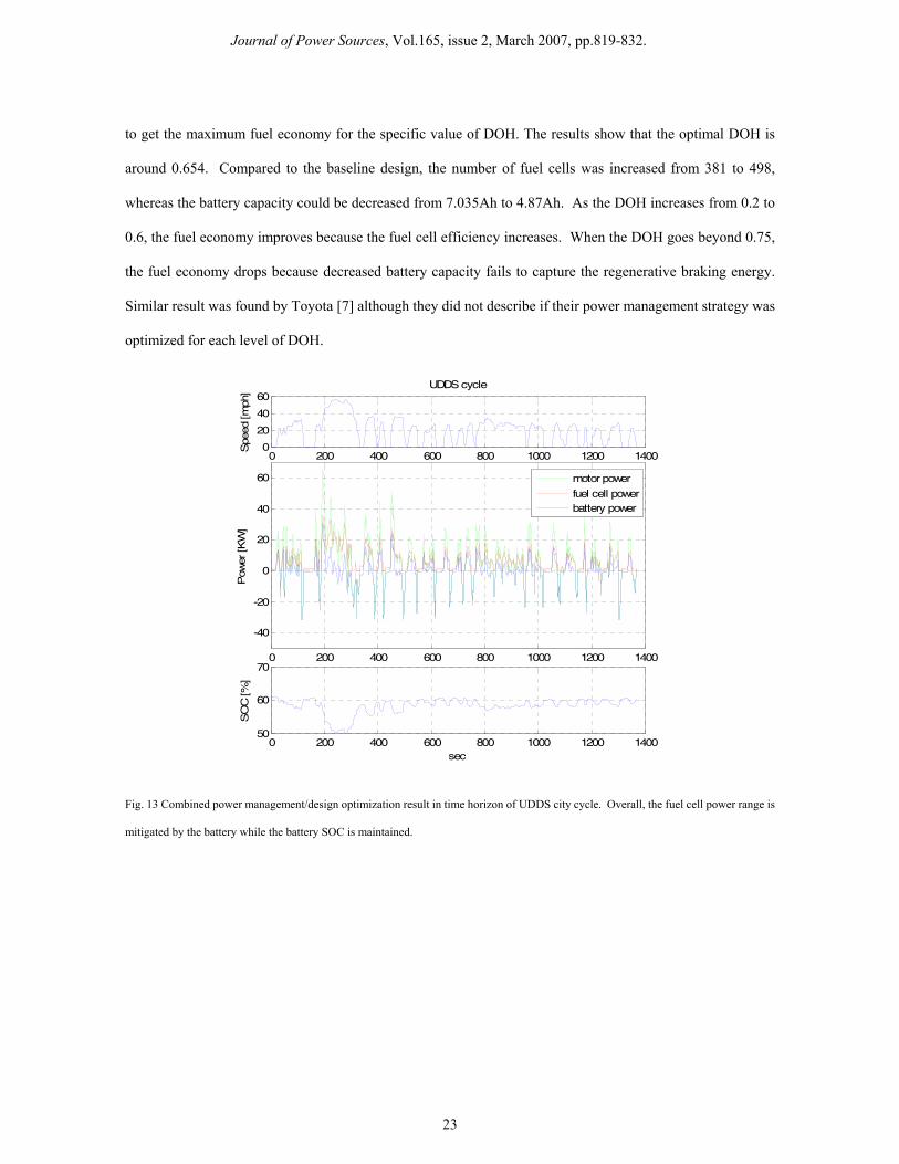
Unlike some strategies that depletes or overcharge the battery, our controller demonstrates that it can
maintain the battery SOC within limited operating range. In Fig. 13, the optimization result in time horizon of
UDDS city cycle was shown. Similar to the original SDP controller, the pseudo SDP controller split the
required motor power to the fuel cell and the battery and maintains the battery SOC.
In Fig. 14, optimization results for city and highway cycles are compared. The city cycle of Fig. 14 (a)
has more accelerations/decelerations so the vehicle can capture more regenerative braking energy. Therefore,
the optimized sensitivity slope of the city cycle is relatively flat compared to that of the highway cycle, i.e.,
* *, ,city highwayx xα α< (Fig. 15). Fig. 14 (b) shows the results for the first 200 seconds of highway cycle, in which the
vehicle is launching and then cruising at 50 mph. When the vehicle first launched, the power demand suddenly
increases and the battery helps to assist power for the FCS, of which the net power rate is limited. When the
vehicle cruises, the pseudo SDP controller runs the FCS “slow and steady” while the battery operates as an
energy buffer to cover the fast dynamics of power demand.
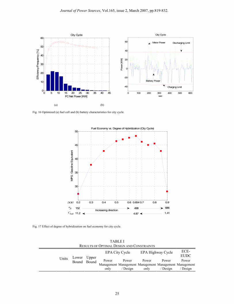
The optimization process downsizes the compressor and increases the DOH. Thus, the FCS efficiency
increases in the lower net power range from 0 to 25KW, where the optimized FC engine primarily operates
(Fig. 16). The maximum efficiency of the optimized FC engine is around 55% where that of the baseline design
in Fig. 7 is around 50%. Although the downsized compressor here reduces the maximum net power of the FCS,
the optimized pseudo SDP controller successfully runs the FCS within the reduced maximum net power limit.
Fig. 16 (b) shows that even though the increased DOH reduces the battery size, the optimized battery design can
still capture the majority of regenerative braking energy within its reduced power limit.
If fuel cell vehicles go into production in the near future, their degree of hybridization will significantly
impact the vehicle price due to high manufacturing and material costs of fuel cells and batteries. Therefore, by
examining the effect of DOH on fuel economy, car manufacturers can determine the trade-off between fuel
savings and manufacturing costs. Fig. 17 illustrates the effect of the DOH on fuel economy for the city cycle.
To obtain each point of the graph, the DOH value is first set, and then other five design variables are optimized
Journal of Power Sources, Vol.165, issue 2, March 2007, pp.819-832.
23
to get the maximum fuel economy for the specific value of DOH. The results show that the optimal DOH is
around 0.654. Compared to the baseline design, the number of fuel cells was increased from 381 to 498,
whereas the battery capacity could be decreased from 7.035Ah to 4.87Ah. As the DOH increases from 0.2 to
0.6, the fuel economy improves because the fuel cell efficiency increases. When the DOH goes beyond 0.75,
the fuel economy drops because decreased battery capacity fails to capture the regenerative braking energy.
Similar result was found by Toyota [7] although they did not describe if their power management strategy was
optimized for each level of DOH.
0 200 400 600 800 1000 1200 14000
20
40
60UDDS cycle
Spe
ed [m
ph]
0 200 400 600 800 1000 1200 1400
-40
-20
0
20
40
60
Pow
er [K
W]
motor power
fuel cell powerbattery power
0 200 400 600 800 1000 1200 140050
60
70
sec
SO
C [%
]
Fig. 13 Combined power management/design optimization result in time horizon of UDDS city cycle. Overall, the fuel cell power range is
mitigated by the battery while the battery SOC is maintained.

Journal of Power Sources, Vol.165, issue 2, March 2007, pp.819-832.
24
350 400 450 500 5500
20
40City cycle
Spe
ed [m
ph]
350 400 450 500 550
-40
-20
0
20
40
60P
ower
[K
W]
350 400 450 500 55055
60
65
sec
SO
C
Motor
Battery
Fuel Cell
(a)
0 50 100 150 2000
20
40
60Highway cycle
Spe
ed [m
ph]
0 50 100 150 200
-40
-20
0
20
40
60
Pow
er [K
W]
motor power
fuel cell powerbattery power
0 50 100 150 20050
55
60
secS
OC
Motor Fuel Cell
Battery
(b)
Fig. 14 Comparison of optimization results for 200 seconds of (a) city cycle (b) highway cycle
18e-006 3.65218e-0063.65218e-006 3.65218e-006
6.866.86
6.86
12.7912.79
12.7912
218.42
18.4218.42
24.1624.16
24.16
30.2130.21
30.21
36.4336.43
SOC
Pow
er D
eman
d [K
W]
City cycle
0.5 0.55 0.6 0.65 0.7-60
-40
-20
0
20
40
60
FC Net Power contour
Vehicle State
4.381
53e-
006
4.381
53e-
006
8.25
8.25
15.17
15.17
21.85
28.83
SOC
Pow
er D
eman
d [K
W]
Highway Cycle
0.5 0.55 0.6 0.65 0.7-60
-40
-20
0
20
40
60
FC Net Power contour
Vehicle State
(a) (b)
Fig. 15 Optimized controller map and vehicle state trajectories (a) city cycle (b) highway cycle. The optimal controller runs the fuel cell
system mostly in the more efficient low power range. The city cycle generates more regenerative braking energy, so its SOC sensitivity
slope of the controller is not as steep as that of the highway cycle.
Journal of Power Sources, Vol.165, issue 2, March 2007, pp.819-832.
25
0 5 10 15 20 25 30 35 40 450
10
20
30
40
50
60
FC Net Power [KW]
Effic
ienc
y/Fre
quen
cy [%
]City Cycle
0 100 200 300 400 500 600
-40
-20
0
20
40
60
sec
Pow
er [K
W]
City Cycle
Discharging Limit
Charging Limit
Battery Power
Motor Power
(a) (b)
Fig. 16 Optimized (a) fuel cell and (b) battery characteristics for city cycle.
0.2 0.3 0.4 0.5 0.6 0.7 0.8 0.90.654
30
35
40
45
50
MP
G G
asol
ine
Equ
ival
ent
Fuel Economy vs. Degree of Hybridization (City Cycle)
DOH
152 686nfc
Cbatt 11.2 1.414.87
498Increasing direction
Fig. 17 Effect of degree of hybridization on fuel economy for city cycle.
TABLE I RESULTS OF OPTIMAL DESIGN AND CONSTRAINTS
EPA City Cycle EPA Highway Cycle ECE- EUDC
Units Lower Bound
Upper Bound Power
Managementonly
Power Management
/ Design
Power Management
only
Power Management
/ Design
Power Management
/ Design

Journal of Power Sources, Vol.165, issue 2, March 2007, pp.819-832.
26
*maxix A/cm2 0.1 2 0.466 0.525 0.521 0.525 0.525 *xα rad 0 1.57 0.238 0.295 0.748 0.954 0.356 *xσ - 0 10 1.25 0.266 2.31 1.25 1.71
*stableSOCx SOC 0.45 0.75 0.625 0.611 0.581 0.582 0.604
*DOHx - 0.2 0.95 0.5# 0.654 0.5# 0.550 0.622
*CPx - 0.5 1.5 1# 0.750 1# 0.866 0.867
g1 max SOC -0.097 -0.127 -0.149 -0.147 -0.114
g2 min SOC -0.024 0 -0.048 -0.026 0
g3 ΔSOC -0.027 -0.367 -0.002 -0.017 -0.001
g4 KW -0.445 -0.011 -.433 -0.260 -0.031
g5 KW/sec -0.051 0 0 0 -0.113
f* MPGGE 41.35 48.35 42.90 44.56 47.56
# : fixed parameters of the baseline design
5. Conclusions
We suggested a comprehensive and systematic framework that makes it possible to optimize power
management and component sizing simultaneously for the future design of FCHVs. To achieve that, we
essentially formulated a combined power management/design optimization problem of a FCHV. To reduce
computational requirement of optimization process, we designed a near-optimal “pseudo SDP controller.”
Unlike heuristic rule-based algorithms, this pseudo SDP controller can generate near-optimal results due to its
similarity to our optimal SDP controller. Because the pseudo SDP controller can be represented with only a few
variables, it can be therefore easily included as design variables in the optimization process. We also presented
subsystem-scaling models that can predict the effect of sizing parameters on the system efficiency
characteristics. Because the compressor size significantly influences the overall efficiency of a fuel cell system,
we mainly focused on it for the fuel cell system scaling model. The combined optimization results show that the
optimality lies in: 1) downsizing the fuel cell compressor; 2) increasing degree of hybridization without
compromising regenerative braking; and 3) employing corresponding control strategy.
REFERENCES

Journal of Power Sources, Vol.165, issue 2, March 2007, pp.819-832.
27
[1] Y. Guezennec, T.-Y. Choi, G. Paganelli, G. Rizzoni , Supervisory Control of Fuel Cell Vehicles and its Link
to Overall System Efficiency and Low-Level Control Requirements, Proceedings of the American Control
Conference, Denver, CO, 2003
[2] P. Rodatz, G. Paganelli, A. Sciarretta, L. Guzzella, Optimal Power Management of an Experimental Fuel
Cell/Supercapacitor-powered Hybrid Vehicle, Control Engineering Practice, Vol. 13, 2005, pp.41-53
[3] A. Sciarretta, L. Guzzella, C. H. Onder, On the Power Split Control of Parallel Hybrid Vehicles: from
Global Optimization towards Real-time Control, Automatisierungstechnik, Vol. 51, 2003, pp.195-203
[4] H. Fathy, J. Reyer, P. Papalambros, A. Ulsoy, On the Coupling between the Plant and Controller
Optimization Problems, Proceedings of the American Control Conference, Arlington, VA, 2001
[5] D. Assanis, G. Delagrammatikas, R. Fellini, Z. Filipi, J. Liedtke, N. Michelena, P. Papalambros, D. Reyes,
D. Rosenbaum, A. Sales, and M. Sasena, An Optimization Approach to Hybrid Electric Propulsion System
Design, Mechanics of Structures and Machines, Vol. 27, No. 4, 1999, pp. 393-421.
[6] R. Fellini, N. Michelena, P. Papalambros, M. Sasena, Optimal Design of Automotive Hybrid Powertrain
Systems, Proceedings of the First International Symposium on Environmentally Conscious Design and
Inverse Manufacturing, Tokyo, Japan, February 1-3, 1999, IEEE Comput. Soc, Los Alamitos, CA, pp.
400-405.
[7] T. Ishikawa, S. Hamaguchi, T. Shimizu, T. Yano, S. Sasaki, K. Kato, M. Ando, H. Yoshida, Development of
Next Generation Fuel-Cell Hybrid System—Consideration of High Voltage System, SAE Paper No.
2004-01-1304
[8] P. Atwood, S. Gurski, D. Nelson, K. Wipke, T. Markel, Degree of Hybridization Modeling of a Hydrogen
Fuel Cell PNGV-Class Vehicle, SAE Paper No. 2002-01-1945
[9] K. Wipke, T. Markel, D. Nelson, Optimizing Energy Management Strategy and Degree of Hybridization for
a Hydrogen Fuel Cell SUV, Proceedings of the 18th Electric Vehicle Symposium, Berlin, Germany, 2003
[10] A. Rousseau, P. Sharer, R. Ahluwalia, Energy Storage Requirements for Fuel Cell Vehicle, SAE Paper No.
2004-01-1302

Journal of Power Sources, Vol.165, issue 2, March 2007, pp.819-832.
28
[11] T. Markel, M. Zolot, K.B. Wipke, A.A. Pesaran, Energy Storage System Requirements for Hybrid Fuel
Cell Vehicles, Proceeding of Advanced Automotive Battery Conference, Nice, France, June, 2003
[12] M.-J. Kim, H. Peng, C.-C. Lin, E. Stamos, D. Tran, Testing, Modeling, and Control of a Fuel Cell Hybrid
Vehicle, Proceedings of the American Control Conference, Portland, OR, 2005
[13] D. D. Boettner, G. Paganelli, Y.G. Guezennec, G. Rizzoni, M.J. Moran, “Proton Exchange Membrane
Fuel Cell System Model for Automotive Vehicle Simulation and Control,” ASME Journal of Energy
Resources Technology, Vol. 124, Issue 1, 2002, pp.20-27
[14] C.-C. Lin, M.-J. Kim, H. Peng, J. Grizzle, System-Level Model and Stochastic Optimal Control for a PEM
Fuel Cell Hybrid Vehicle, ASME Journal of Dynamic Systems, Measurement, and Control (to be appeared)
[15] J.P. Jensen, A.F. Kristensen, S.C. Sorenson, N. Houbak, E. Hendricks, Mean Value Modeling of a Small
Turbocharged Diesel Engine, SAE910070
[16] USDOE, FreedomCAR Battery Test Manual for Power-Assist Hybrid Electric Vehicles, DOE/ID-11069,
Contract DE-AC07-99-ID13727, October, 2003
[17] D.R.Jones, C.D. Perttunen, B.E. Stuckman, Lipschitzian Optimization Without the Lipschitz Constant,
Journal of Optimization Theory and Application, 79(1), pp.157-181, October 1993.
Nomenclature
C = capacity of battery
d = diameter
F = Faraday’s number
I = current (A) k = motor parameter
m = mass (kg)
M = molecular mass (kg/mol)
fcn = number of fuel cells
P = Power (Watt) p = pressure (Pa) or probability

Journal of Power Sources, Vol.165, issue 2, March 2007, pp.819-832.
29
R = gas constant or resistance ( Ω )
T = temperature (K)
y = mole fraction η = efficiency
u = control input
V = voltage (V)
v = longitudinal speed (m/s)
Vol = volume (m3)
W = mass flow rate (kg/s)
w = random parameter
x = design variable
α = sensitivity slope in controller
Φ = non-dimensional compressor diameter
ω = rotational speed (rad/s)
λ = excess ratio φ = relative humidity
ψ = humidity ratio
τ = torque (N-m) γ = air specific heat ratio or discount factor
ρ = density (kg/m3)
Subscripts:
a = air
amb = ambient
an = anode
aux = auxiliary
batt = battery
ca = cathode
cm = compressor motor cp = compressor
cr = corrected
dcdc = DC/DC converter fc = fuel cell

Journal of Power Sources, Vol.165, issue 2, March 2007, pp.819-832.
30
hm = humidifier
in = inlet
m = traction motor
out = outlet
oc = open circuit
rct = reacted req = requested
sat = saturation
sm = supply manifold
st = fuel cell stack
t = terminal
v = vapor
veh = vehicle
wh = wheel
Acronyms:
DC/DC = Direct Current to Direct Current converter
FCHV = Fuel Cell Hybrid Vehicle
FC-VESIM = Fuel Cell Hybrid Vehicle Simulation Model
HEV = Hybrid Electric Vehicle
PEM = Proton Exchange Membrane
PWM = Pulse Width Modulator
SDP = Stochastic Dynamic Programming
SOC = State of Charge