Power Laws and Preferential...
122
. . . . . . . . . . . . . . . . . . . . . . . . . . . . . . . . . . . . . . . . Power Laws and Preferential Attachment Web Science (VU) (707.000) Denis Helic KTI, TU Graz June 1, 2017 Denis Helic (KTI, TU Graz) PL-PA June 1, 2017 1 / 111
Transcript of Power Laws and Preferential...

...
.
...
.
...
.
...
.
...
.
...
.
...
.
...
.
...
.
...
.
Power Laws and Preferential AttachmentWeb Science (VU) (707.000)
Denis Helic
KTI, TU Graz
June 1, 2017
Denis Helic (KTI, TU Graz) PL-PA June 1, 2017 1 / 111

...
.
...
.
...
.
...
.
...
.
...
.
...
.
...
.
...
.
...
.
Outline
1 Popularity
2 A Simple Hypothesis
3 Log-normal Distributions
4 Power Laws
5 Rich-Get-Richer Models
6 Preferential Attachment
7 Multiplicative Random Processes
8 Self-Organized Criticality
9 Optimization Processes
Denis Helic (KTI, TU Graz) PL-PA June 1, 2017 2 / 111

...
.
...
.
...
.
...
.
...
.
...
.
...
.
...
.
...
.
...
.
Popularity
Popularity
Denis Helic (KTI, TU Graz) PL-PA June 1, 2017 3 / 111

...
.
...
.
...
.
...
.
...
.
...
.
...
.
...
.
...
.
...
.
Popularity
Popularity
Popularity is a phenomenon characterized by extreme imbalancesAlmost everyone is known only to people in their immediate socialcirclesA few people achieve wider visibilityA very few attain global name recognitionAnalogy with books, movies, scientific papersEverything that requires an audience
Denis Helic (KTI, TU Graz) PL-PA June 1, 2017 4 / 111

...
.
...
.
...
.
...
.
...
.
...
.
...
.
...
.
...
.
...
.
Popularity
Popularity: questions
How can we quantify imbalances?
Analyze distributionsWhy do these imbalances arise?What are the mechanisms and processes that cause them?Are they intrinsic (generalizable, universal) to popularity?
Denis Helic (KTI, TU Graz) PL-PA June 1, 2017 5 / 111
...
.
...
.
...
.
...
.
...
.
...
.
...
.
...
.
...
.
...
.
Popularity
Popularity: questions
How can we quantify imbalances?Analyze distributionsWhy do these imbalances arise?What are the mechanisms and processes that cause them?Are they intrinsic (generalizable, universal) to popularity?
Denis Helic (KTI, TU Graz) PL-PA June 1, 2017 5 / 111

...
.
...
.
...
.
...
.
...
.
...
.
...
.
...
.
...
.
...
.
Popularity
Web as an example
To begin the analysis we take the Web as an exampleOn the Web it is easy to measure popularity very accuratelyE.g. it is difficult to estimate the number of people worldwide whohave heard of Bill GatesHow can we achieve this on the Web?
Take a snapshot of the Web and count the number of in-links to BillGates homepageCalculate the authority score of Bill Gates homepageCalculate the PageRank of Bill Gates homepageWe will learn how to calculate these quantities later in the course
Denis Helic (KTI, TU Graz) PL-PA June 1, 2017 6 / 111

...
.
...
.
...
.
...
.
...
.
...
.
...
.
...
.
...
.
...
.
Popularity
Web as an example
To begin the analysis we take the Web as an exampleOn the Web it is easy to measure popularity very accuratelyE.g. it is difficult to estimate the number of people worldwide whohave heard of Bill GatesHow can we achieve this on the Web?Take a snapshot of the Web and count the number of in-links to BillGates homepageCalculate the authority score of Bill Gates homepageCalculate the PageRank of Bill Gates homepageWe will learn how to calculate these quantities later in the course
Denis Helic (KTI, TU Graz) PL-PA June 1, 2017 6 / 111

...
.
...
.
...
.
...
.
...
.
...
.
...
.
...
.
...
.
...
.
Popularity
The popularity question: a basic version
As a function of 𝑘, what fraction of pages on the Web have 𝑘 in-linksLarger values of 𝑘 indicate greater popularityTechnically, what is the question about?
Distribution of the number of in-links (in-degree distribution) over aset of Web pagesWhat is the interpretation of this question/answer?Distribution of popularity over a set of Web pages
Denis Helic (KTI, TU Graz) PL-PA June 1, 2017 7 / 111

...
.
...
.
...
.
...
.
...
.
...
.
...
.
...
.
...
.
...
.
Popularity
The popularity question: a basic version
As a function of 𝑘, what fraction of pages on the Web have 𝑘 in-linksLarger values of 𝑘 indicate greater popularityTechnically, what is the question about?Distribution of the number of in-links (in-degree distribution) over aset of Web pagesWhat is the interpretation of this question/answer?
Distribution of popularity over a set of Web pages
Denis Helic (KTI, TU Graz) PL-PA June 1, 2017 7 / 111

...
.
...
.
...
.
...
.
...
.
...
.
...
.
...
.
...
.
...
.
Popularity
The popularity question: a basic version
As a function of 𝑘, what fraction of pages on the Web have 𝑘 in-linksLarger values of 𝑘 indicate greater popularityTechnically, what is the question about?Distribution of the number of in-links (in-degree distribution) over aset of Web pagesWhat is the interpretation of this question/answer?Distribution of popularity over a set of Web pages
Denis Helic (KTI, TU Graz) PL-PA June 1, 2017 7 / 111

...
.
...
.
...
.
...
.
...
.
...
.
...
.
...
.
...
.
...
.
A Simple Hypothesis
A Simple Hypothesis
Denis Helic (KTI, TU Graz) PL-PA June 1, 2017 8 / 111

...
.
...
.
...
.
...
.
...
.
...
.
...
.
...
.
...
.
...
.
A Simple Hypothesis
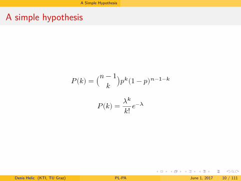
A simple hypothesis
Before trying to resolve the questionWhat do we expect the answer to be?What distribution do we expect?What was the degree distribution in the random graph 𝐺(𝑛, 𝑝)?
Binomial and approximation was Poisson
Denis Helic (KTI, TU Graz) PL-PA June 1, 2017 9 / 111

...
.
...
.
...
.
...
.
...
.
...
.
...
.
...
.
...
.
...
.
A Simple Hypothesis
A simple hypothesis
Before trying to resolve the questionWhat do we expect the answer to be?What distribution do we expect?What was the degree distribution in the random graph 𝐺(𝑛, 𝑝)?Binomial and approximation was Poisson
Denis Helic (KTI, TU Graz) PL-PA June 1, 2017 9 / 111
...
.
...
.
...
.
...
.
...
.
...
.
...
.
...
.
...
.
...
.
A Simple Hypothesis
A simple hypothesis
𝑃(𝑘) = (𝑛 − 1𝑘 )𝑝𝑘(1 − 𝑝)𝑛−1−𝑘
𝑃(𝑘) = 𝜆𝑘
𝑘! 𝑒−𝜆
Denis Helic (KTI, TU Graz) PL-PA June 1, 2017 10 / 111

...
.
...
.
...
.
...
.
...
.
...
.
...
.
...
.
...
.
...
.
A Simple Hypothesis
Degree distribution (Binomial)
0 1 2 3 4 5 6 7 8 9 10 11 12 13 14 15 16 17 18 19 20k
0.00
0.05
0.10
0.15
0.20
0.25
0.30p(k
)Degree distribution random graph (n= 21); differing p values
p= 0. 10
p= 0. 40
Denis Helic (KTI, TU Graz) PL-PA June 1, 2017 11 / 111

...
.
...
.
...
.
...
.
...
.
...
.
...
.
...
.
...
.
...
.
A Simple Hypothesis
Degree distribution (Poisson)
0 1 2 3 4 5 6 7 8 9 10 11 12 13 14 15 16 17 18 19 20k
0.00
0.05
0.10
0.15
0.20
0.25
0.30p(k
)Degree distribution random graph (n= 21); differing λ values
λ= 2. 0
λ= 8. 0
Denis Helic (KTI, TU Graz) PL-PA June 1, 2017 12 / 111

...
.
...
.
...
.
...
.
...
.
...
.
...
.
...
.
...
.
...
.
A Simple Hypothesis
Degree distribution (Poisson approximation)
0 1 2 3 4 5 6 7 8 9 10 11 12 13 14 15 16 17 18 19 20k
0.00
0.02
0.04
0.06
0.08
0.10
0.12
0.14
0.16
0.18p(k
)Degree distribution random graph (n= 21); Poisson approx. binomial
p= 0. 40
λ= 8. 0
Denis Helic (KTI, TU Graz) PL-PA June 1, 2017 13 / 111

...
.
...
.
...
.
...
.
...
.
...
.
...
.
...
.
...
.
...
.
A Simple Hypothesis
A simple hypothesis
From our experience how are some typical quantities distributed inour world?People’s height, weight, and strengthIn engineering and natural sciencesErrors of measurement, position and velocities of particles in variousphysical processes, etc.Continuous approximation of Binomial and Poisson: NormalDistribution
Denis Helic (KTI, TU Graz) PL-PA June 1, 2017 14 / 111

...
.
...
.
...
.
...
.
...
.
...
.
...
.
...
.
...
.
...
.
A Simple Hypothesis
Normal (Gaussian) distribution
It occurs so often in nature, engineering and society: NormalCharacterized by a mean value 𝜇 and a standard deviation around themean 𝜎
𝑓(𝑥) = 1√2𝜋𝜎2 𝑒− (𝑥−𝜇)2
2𝜎2
CDF
𝐹(𝑥) = Φ(𝑥 − 𝜇𝜎 ), Φ(𝑥) = 1√
2𝜋 ∫𝑥
−∞𝑒− 𝑥′2
2 𝑑𝑥′
Denis Helic (KTI, TU Graz) PL-PA June 1, 2017 15 / 111

...
.
...
.
...
.
...
.
...
.
...
.
...
.
...
.
...
.
...
.
A Simple Hypothesis
Normal (Gaussian) distribution
10 5 0 5 10x
0.00
0.05
0.10
0.15
0.20
0.25
0.30
0.35
0.40pr
obab
ility
of x
PDF of a Normal random variable; differing µ and σ values
µ=0.0,σ=1.0
µ=−2.0,σ=2.0
Denis Helic (KTI, TU Graz) PL-PA June 1, 2017 16 / 111

...
.
...
.
...
.
...
.
...
.
...
.
...
.
...
.
...
.
...
.
A Simple Hypothesis
Standard normal distribution
If 𝜇 = 0 and 𝜎 = 1 we talk about standard normal distribution
𝑓(𝑥) = 1√2𝜋𝑒− 𝑥2
2
Please note, that you can always standardize a random variable 𝑋with:
Standardizing
𝑍 = 𝑋 − 𝜇𝜎
Denis Helic (KTI, TU Graz) PL-PA June 1, 2017 17 / 111

...
.
...
.
...
.
...
.
...
.
...
.
...
.
...
.
...
.
...
.
A Simple Hypothesis
Normal (Gaussian) distribution
The basic fact: the probability of observing a value that exceed meanby more than 𝑐 times the standard deviation decreases exponentiallyin 𝑐
𝑟(1) = 𝑓(1)𝑓(0) = �
��1√2𝜋 𝑒−1/2
���1√2𝜋
= 1√𝑒 ≈ 0.6
𝑟(𝑐𝜎) = 𝑟(𝑐) = 𝑓(𝑐)𝑓(0) = �
��1√2𝜋 𝑒−𝑐2/2
���1√2𝜋
= 𝑒−𝑐2/2 = 𝑂(𝑒−𝑐)Denis Helic (KTI, TU Graz) PL-PA June 1, 2017 18 / 111

...
.
...
.
...
.
...
.
...
.
...
.
...
.
...
.
...
.
...
.
A Simple Hypothesis
Normal (Gaussian) distribution
Why is normal distribution so ubiquitousTheoretical result: Central Limit Theorem provides an explanationInformally, we take any sequence of small independent and identicallydistributed (i.i.d) random quantitiesIn the limit of infinitely long sequences their sum (or their average)are distributed normally
Denis Helic (KTI, TU Graz) PL-PA June 1, 2017 19 / 111
...
.
...
.
...
.
...
.
...
.
...
.
...
.
...
.
...
.
...
.
A Simple Hypothesis
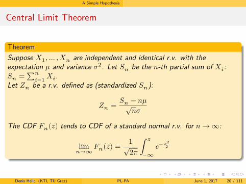
Central Limit Theorem
TheoremSuppose 𝑋1, … , 𝑋𝑛 are independent and identical r.v. with theexpectation 𝜇 and variance 𝜎2. Let 𝑆𝑛 be the 𝑛-th partial sum of 𝑋𝑖:𝑆𝑛 = ∑𝑛
𝑖=1 𝑋𝑖.Let 𝑍𝑛 be a r.v. defined as (standardized 𝑆𝑛):
𝑍𝑛 = 𝑆𝑛 − 𝑛𝜇√𝑛𝜎
The CDF 𝐹𝑛(𝑧) tends to CDF of a standard normal r.v. for 𝑛 → ∞:
lim𝑛→∞
𝐹𝑛(𝑧) = 1√2𝜋 ∫
𝑧
−∞𝑒− 𝑥2
2
Denis Helic (KTI, TU Graz) PL-PA June 1, 2017 20 / 111

...
.
...
.
...
.
...
.
...
.
...
.
...
.
...
.
...
.
...
.
A Simple Hypothesis
Central Limit Theorem
10 5 0 5 100.00
0.05
0.10
0.15
0.20
0.25
0.30
0.35
0.40
0.45
µ= 0. 0, σ= 1. 0
Z30
Central limit theorem with unif. dist. and Z30: µ= − 0. 007, σ2 = 1. 00474
Denis Helic (KTI, TU Graz) PL-PA June 1, 2017 21 / 111

...
.
...
.
...
.
...
.
...
.
...
.
...
.
...
.
...
.
...
.
A Simple Hypothesis
Central Limit Theorem
10 5 0 5 100.00
0.05
0.10
0.15
0.20
0.25
0.30
0.35
0.40
0.45
µ= 0. 0, σ= 1. 0
Z100
Central limit theorem with unif. dist. and Z100: µ= 0. 001, σ2 = 0. 99159
Denis Helic (KTI, TU Graz) PL-PA June 1, 2017 22 / 111

...
.
...
.
...
.
...
.
...
.
...
.
...
.
...
.
...
.
...
.
A Simple Hypothesis
Central Limit Theorem: Proof
Now we present a proof sketch (to better understand the assumptionsthat CLT makes)For the proof we need some preliminaries
DefinitionCharacteristic function of a real valued r.v. 𝑋 is defined as expectation ofthe complex function 𝑒𝑖𝑡𝑋:
𝜑𝑋(𝑡) = 𝐸[𝑒𝑖𝑡𝑋] = ∫∞
−∞𝑒𝑖𝑡𝑥𝑓(𝑥)𝑑𝑥,
where 𝑡 is the parameter and 𝑓(𝑥) is PDF of r.v. 𝑋.
A characteristic function completely defines PDF of a r.v.
Denis Helic (KTI, TU Graz) PL-PA June 1, 2017 23 / 111

...
.
...
.
...
.
...
.
...
.
...
.
...
.
...
.
...
.
...
.
A Simple Hypothesis
Central Limit Theorem: Proof
To calculate characteristic function we typically apply Taylorexpansion:
𝑒𝑖𝑡𝑋 =∞∑𝑛=0
(𝑖𝑡𝑥)𝑛
𝑛!
= 1 + 𝑖𝑡𝑥 − (𝑡𝑥)2
2 + 𝑂(𝑡3)
Denis Helic (KTI, TU Graz) PL-PA June 1, 2017 24 / 111

...
.
...
.
...
.
...
.
...
.
...
.
...
.
...
.
...
.
...
.
A Simple Hypothesis
Central Limit Theorem: Proof
Substituting the expansion into the integral:
𝜑𝑋(𝑡) = ∫∞
−∞𝑓(𝑥)𝑑𝑥 + ∫
∞
−∞𝑖𝑡𝑥𝑓(𝑥)𝑑𝑥 − ∫
∞
−∞
(𝑡𝑥)2
2 𝑓(𝑥)𝑑𝑥 + 𝑂(𝑡3)
= 1 + 𝑖𝑡𝐸[𝑋] − (𝑡𝑥)2
2 𝐸[𝑋2] + 𝑂(𝑡3)
Now suppose that we have a r.v. 𝑋 with 0 mean and variance 1(which can be always achieved by standardizing a r.v. with finitemean and variance):
𝜑𝑋(𝑡) = 1 − (𝑡𝑥)2
2 + 𝑂(𝑡3)
Denis Helic (KTI, TU Graz) PL-PA June 1, 2017 25 / 111

...
.
...
.
...
.
...
.
...
.
...
.
...
.
...
.
...
.
...
.
A Simple Hypothesis
Central Limit Theorem: Proof
Another important fact of the characteristic functionsSuppose 𝑋 and 𝑌 are two independent r.v.We want to calculate the characteristic function of r.v. 𝑍 = 𝑋 + 𝑌 :
𝜑𝑋+𝑌 (𝑡) = 𝐸[𝑒𝑖𝑡(𝑋+𝑌 )] = 𝐸[𝑒𝑖𝑡𝑋𝑒𝑖𝑡𝑌 ] = 𝐸[𝑒𝑖𝑡𝑋]𝐸[𝑒𝑖𝑡𝑌 ]= 𝜑𝑋(𝑡)𝜑𝑌 (𝑡)
Last equality in the first row follows from the independenceThe last fact that we need: if 𝑍 ∼ 𝑁(0, 1) then 𝜑𝑍(𝑡) = 𝑒−𝑡2/2
Denis Helic (KTI, TU Graz) PL-PA June 1, 2017 26 / 111

...
.
...
.
...
.
...
.
...
.
...
.
...
.
...
.
...
.
...
.
A Simple Hypothesis
Central Limit Theorem: Proof
Suppose now we have a set of random variables with individual𝑋𝑖 ∼ (𝜇, 𝜎2) which are all independent and identically distributed(i.i.d.)Note that we do not make assumptions on the distribution of 𝑋𝑖 justthat they have finite 𝜇 and 𝜎2
We build a new r.v. 𝑆𝑛 = ∑𝑛𝑖=1 𝑋𝑖 as the 𝑛-th partial sum
𝐸[𝑆𝑛] =𝑛
∑𝑖=1
𝐸[𝑋𝑖] =𝑛
∑𝑖=1
𝜇 = 𝑛𝜇
𝑉 𝑎𝑟(𝑆𝑛) =𝑛
∑𝑖=1
𝑉 𝑎𝑟(𝑋𝑖) =𝑛
∑𝑖=1
𝜎2 = 𝑛𝜎2
Denis Helic (KTI, TU Graz) PL-PA June 1, 2017 27 / 111

...
.
...
.
...
.
...
.
...
.
...
.
...
.
...
.
...
.
...
.
A Simple Hypothesis
Central Limit Theorem: Proof
Now we standardize 𝑆𝑛 to obtain 𝑍𝑛:
𝑍𝑛 = 𝑆𝑛 − 𝐸[𝑆𝑛]√𝑉 𝑎𝑟(𝑆𝑛)
= 𝑆𝑛 − 𝑛𝜇√𝑛𝜎 =∑𝑛
𝑖=1(𝑋𝑖 − 𝜇)√𝑛𝜎
By introducing 𝑌𝑖 = 𝑋𝑖−𝜇𝜎 (please note that 𝑌𝑖 is standardization of
𝑋𝑖, i.e. 𝑌𝑖 ∼ (0, 1):
𝑍𝑛 =∑𝑛
𝑖=1 𝑌𝑖√𝑛
Denis Helic (KTI, TU Graz) PL-PA June 1, 2017 28 / 111

...
.
...
.
...
.
...
.
...
.
...
.
...
.
...
.
...
.
...
.
A Simple Hypothesis
Central Limit Theorem: Proof
Now let us calculate 𝜑𝑍𝑛(𝑡) (where we use the fact that characteristic
function of the sum equals to the product of characteristic functionsif r.v. are independent and we scale the parameter 𝑡 with 1/√𝑛):
𝜑𝑍𝑛=
𝑛∏𝑖=1
𝜑𝑌𝑖(𝑡/√𝑛) = [𝜑𝑌 (𝑡/√𝑛)]𝑛
= [1 − 𝑡2
2𝑛 + 𝑂((𝑡/√𝑛)3)]𝑛
Denis Helic (KTI, TU Graz) PL-PA June 1, 2017 29 / 111

...
.
...
.
...
.
...
.
...
.
...
.
...
.
...
.
...
.
...
.
A Simple Hypothesis
Central Limit Theorem: Proof
Now we are interested what happens when 𝑛 → ∞Obviously 𝑂((𝑡/√𝑛)3) → 0Thus, we have:
lim𝑛→∞
𝜑𝑍𝑛= lim
𝑛→∞[1 − 𝑡2
2𝑛]𝑛 = 𝑒−𝑡2/2
We obtain the characteristic function of standard normal and thuslim𝑛→∞ 𝑍𝑛 ∼ 𝑁(0, 1)
Denis Helic (KTI, TU Graz) PL-PA June 1, 2017 30 / 111

...
.
...
.
...
.
...
.
...
.
...
.
...
.
...
.
...
.
...
.
A Simple Hypothesis
Central Limit Theorem
How can we interpret this result?
Any quantity that can be viewed as a sum of many small independentrandom effects will have a normal distributionE.g. we take a lot of measurements of a fixed physical quantityVariations in the measurements across trials are cumulative results ofmany independent sources of errorsE.g. errors in the equipment, human errors, changes in externalfactorsThen the distribution of measured values is normally distributed
Denis Helic (KTI, TU Graz) PL-PA June 1, 2017 31 / 111

...
.
...
.
...
.
...
.
...
.
...
.
...
.
...
.
...
.
...
.
A Simple Hypothesis
Central Limit Theorem
How can we interpret this result?Any quantity that can be viewed as a sum of many small independentrandom effects will have a normal distributionE.g. we take a lot of measurements of a fixed physical quantityVariations in the measurements across trials are cumulative results ofmany independent sources of errorsE.g. errors in the equipment, human errors, changes in externalfactorsThen the distribution of measured values is normally distributed
Denis Helic (KTI, TU Graz) PL-PA June 1, 2017 31 / 111

...
.
...
.
...
.
...
.
...
.
...
.
...
.
...
.
...
.
...
.
A Simple Hypothesis
Central Limit Theorem
Can you explain why examination grades tend to be normallydistributed?
Each student is a small “random factor”The points for each question are a random variable, which are i.i.dThen the sum (average) of the points will be according to CLTnormally distributedIf the distribution of exam grades for a course is not normal what canbe going on?Too strict, too loose, discrimination, independence is broken, notidentically distributed, etc.
Denis Helic (KTI, TU Graz) PL-PA June 1, 2017 32 / 111
...
.
...
.
...
.
...
.
...
.
...
.
...
.
...
.
...
.
...
.
A Simple Hypothesis
Central Limit Theorem
Can you explain why examination grades tend to be normallydistributed?Each student is a small “random factor”The points for each question are a random variable, which are i.i.dThen the sum (average) of the points will be according to CLTnormally distributedIf the distribution of exam grades for a course is not normal what canbe going on?
Too strict, too loose, discrimination, independence is broken, notidentically distributed, etc.
Denis Helic (KTI, TU Graz) PL-PA June 1, 2017 32 / 111

...
.
...
.
...
.
...
.
...
.
...
.
...
.
...
.
...
.
...
.
A Simple Hypothesis
Central Limit Theorem
Can you explain why examination grades tend to be normallydistributed?Each student is a small “random factor”The points for each question are a random variable, which are i.i.dThen the sum (average) of the points will be according to CLTnormally distributedIf the distribution of exam grades for a course is not normal what canbe going on?Too strict, too loose, discrimination, independence is broken, notidentically distributed, etc.
Denis Helic (KTI, TU Graz) PL-PA June 1, 2017 32 / 111

...
.
...
.
...
.
...
.
...
.
...
.
...
.
...
.
...
.
...
.
A Simple Hypothesis
How to apply this on the Web?
If we model the link structure by assuming that each page decidesindependently at random to which page to link toThen the number of in-links for any given page is the sum of manyi.i.d quantitiesHence, we expect it to be normally distributedIf we believe that this model is correct:Then the number of pages with 𝑘 in-links should decreaseexponentially in 𝑘 as 𝑘 grows
Denis Helic (KTI, TU Graz) PL-PA June 1, 2017 33 / 111

...
.
...
.
...
.
...
.
...
.
...
.
...
.
...
.
...
.
...
.
Log-normal Distributions
Log-Normal Distribution
Denis Helic (KTI, TU Graz) PL-PA June 1, 2017 34 / 111

...
.
...
.
...
.
...
.
...
.
...
.
...
.
...
.
...
.
...
.
Log-normal Distributions
Log-Normal Distribution
If 𝑋 is log-normally distributed ⇔ 𝑌 = 𝑙𝑛(𝑋) is normally distributedIf 𝑌 is normally distributed ⇔ 𝑋 = 𝑒𝑌 is log-normally distributedCharacterized by a mean value 𝜇 and a standard deviation around themean 𝜎
𝑓(𝑥) = 1𝑥𝜎
√2𝜋𝑒− (𝑙𝑛(𝑥)−𝜇)2
2𝜎2
Denis Helic (KTI, TU Graz) PL-PA June 1, 2017 35 / 111

...
.
...
.
...
.
...
.
...
.
...
.
...
.
...
.
...
.
...
.
Log-normal Distributions
Log-Normal Distribution
0 1 2 3 4 5x
0.0
0.2
0.4
0.6
0.8
1.0
1.2
1.4
1.6
1.8p(x
)PDF of a Log-Normal random variable; differing µ and σ values
µ= 0. 00, σ= 0. 25
µ= 0. 00, σ= 1. 00
Denis Helic (KTI, TU Graz) PL-PA June 1, 2017 36 / 111

...
.
...
.
...
.
...
.
...
.
...
.
...
.
...
.
...
.
...
.
Log-normal Distributions
Multiplicative random processes
Multiplicative random processes lead to log-normal distributionsSuppose we have a set of random variables with individual𝑋𝑖 ∼ (𝜇, 𝜎2) which are all independent and identically distributed(i.i.d.)Note that we do not make assumptions on the distribution of 𝑋𝑖 justthat they have finite 𝜇 and 𝜎2
We build a new r.v. 𝑃𝑛 = ∏𝑛𝑖=1 𝑋𝑖 as the 𝑛-th partial product
We claim that lim𝑛→∞ 𝑃𝑛 is log-normally distributed
Denis Helic (KTI, TU Graz) PL-PA June 1, 2017 37 / 111

...
.
...
.
...
.
...
.
...
.
...
.
...
.
...
.
...
.
...
.
Log-normal Distributions
Multiplicative random processes
𝑃𝑛 =𝑛
∏𝑖=1
𝑋𝑖
𝑙𝑛(𝑃𝑛) =𝑛
∑𝑖=1
𝑙𝑛(𝑋𝑖)
From the CLT we now that 𝑙𝑛(𝑃𝑛) tends to standard normalThus, 𝑃𝑛 tends to log-normal distribution
Denis Helic (KTI, TU Graz) PL-PA June 1, 2017 38 / 111

...
.
...
.
...
.
...
.
...
.
...
.
...
.
...
.
...
.
...
.
Power Laws
Power Laws
Denis Helic (KTI, TU Graz) PL-PA June 1, 2017 39 / 111

...
.
...
.
...
.
...
.
...
.
...
.
...
.
...
.
...
.
...
.
Power Laws
Power Laws
When people measured the distribution of links on the Web theyfound something very different to Normal distributionIn all studies over many different Web snapshots:The fraction of Web pages that have 𝑘 in-links is approximatelyproportional to 1/𝑘2
More precisely the exponent on 𝑘 is slightly larger than 2
Denis Helic (KTI, TU Graz) PL-PA June 1, 2017 40 / 111

...
.
...
.
...
.
...
.
...
.
...
.
...
.
...
.
...
.
...
.
Power Laws
Power Laws
What is the difference to the normal distribution?1/𝑘2 decreases much more slowly as 𝑘 increasesPages with large number of in-links are much more common than wewould expect with a normal distributionE.g. 1/𝑘2 for 𝑘 = 1000 is one in millionOne page in million will have 1000 in-linksFor a function like 𝑒−𝑘 or 2−𝑘 this is unimaginably smallNo page will have 1000 in-links
Denis Helic (KTI, TU Graz) PL-PA June 1, 2017 41 / 111

...
.
...
.
...
.
...
.
...
.
...
.
...
.
...
.
...
.
...
.
Power Laws
Power Laws
A function that decreases as 𝑘 to some fixed power 1/𝑘𝑐, e.g. 1/𝑘2 iscalled power lawThe basic property: it is possible to see very large values of 𝑘This is a quantitative explanation of popularity imbalanceIt accords to our intuition for the Web: there is a reasonable largenumber of extremely popular Web pagesWe observe similar power laws in many other domainsThe fraction of books that are bought by 𝑘 people: 1/𝑘3
The fraction of scientific papers that receive 𝑘 citations: 1/𝑘3, etc.
Denis Helic (KTI, TU Graz) PL-PA June 1, 2017 42 / 111

...
.
...
.
...
.
...
.
...
.
...
.
...
.
...
.
...
.
...
.
Power Laws
Power Laws
The normal distribution is widespread in natural sciences andengineeringPower laws seem to dominate whenever popularity is involved, i.e.(informally) in social sciences and/or e.g. psychologyConclusion: if you analyze the user data of any kindE.g. the number of downloads, the number of emails, the number oftweetsExpect to see a power lawTest for power law: histogram + test if 1/𝑘𝑐 for some 𝑐If yes estimate 𝑐
Denis Helic (KTI, TU Graz) PL-PA June 1, 2017 43 / 111

...
.
...
.
...
.
...
.
...
.
...
.
...
.
...
.
...
.
...
.
Power Laws
Power Law Histogram
0 1 2 3 4 5 6 7 8 9 10 11 12 13 14 15 16 17 18 19k
0.0
0.1
0.2
0.3
0.4
0.5
0.6
0.7
0.8
0.9p(k
)PMF of a power law r. v.; differing c values
c= 2. 0
c= 3. 0
Denis Helic (KTI, TU Graz) PL-PA June 1, 2017 44 / 111

...
.
...
.
...
.
...
.
...
.
...
.
...
.
...
.
...
.
...
.
Power Laws
Power Law check: a simple method
A simple visual methodLet 𝑓(𝑘) be the fraction of items that have value 𝑘We want to know id 𝑓(𝑘) = 𝑎/𝑘𝑐 approximately holds for someexponent 𝑐 and some proportion constant 𝑎Let us take the logarithms of both sides
𝑙𝑛(𝑓(𝑘)) = 𝑙𝑛(𝑎) − 𝑐 ⋅ 𝑙𝑛(𝑘)
Denis Helic (KTI, TU Graz) PL-PA June 1, 2017 45 / 111

...
.
...
.
...
.
...
.
...
.
...
.
...
.
...
.
...
.
...
.
Power Laws
Power Law Log-Log Plot
0 1 2 3 4 5 6 7 8 9k
10-3
10-2
10-1
100p(k
)PMF of a power law r. v.; differing c values
c= 2. 0
c= 3. 0
Denis Helic (KTI, TU Graz) PL-PA June 1, 2017 46 / 111

...
.
...
.
...
.
...
.
...
.
...
.
...
.
...
.
...
.
...
.
Power Laws
Power Law check: a simple method
If we plot 𝑓(𝑘) on a log-log scale we expect to see a straight line−𝑐 is the slop and 𝑙𝑛(𝑎) will be the 𝑦-interceptThis is only a simple check to see if there is an apparent power lawbehaviorDo not use this method to estimate the parameters!There are statistically sound methods to thatWe discuss them in some other courses e.g. Network Science
Denis Helic (KTI, TU Graz) PL-PA June 1, 2017 47 / 111

...
.
...
.
...
.
...
.
...
.
...
.
...
.
...
.
...
.
...
.
Power Laws
Power Law check: a simple method546 CHAPTER 18. POWER LAWS AND RICH-GET-RICHER PHENOMENA
Figure 18.2: A power law distribution (such as this one for the number of Web page in-links,from Broder et al. [80]) shows up as a straight line on a log-log plot.
in total is roughly proportional to 1/k3; and there are many related examples [10, 320].
Indeed, just as the normal distribution is widespread in a family of settings in the natural
sciences, power laws seem to dominate in cases where the quantity being measured can be
viewed as a type of popularity. Hence, if you are handed data of this sort — say, for example,
that someone gives you a table showing the number of monthly downloads for each song at
a large on-line music site that they’re hosting — one of the first things that’s worth doing
is to test whether it’s approximately a power law 1/kc for some c, and if so, to estimate the
exponent c.
There’s a simple method that provides at least a quick test for whether a dataset exhibits
a power-law distribution. Let f(k) be the fraction of items that have value k, and suppose you
want to know whether the equation f(k) = a/kc approximately holds, for some exponent
c and constant of proportionality a. Then, if we write this as f(k) = ak−c and take the
logarithms of both sides of this equation, we get
log f(k) = log a− c log k.
This says that if we have a power-law relationship, and we plot log f(k) as a function of log k,
then we should see a straight line: −c will be the slope, and log a will be the y-intercept.
Such a “log-log” plot thus provides a quick way to see if one’s data exhibits an approximate
power-law: it is easy to see if one has an approximately straight line, and one can read off
the exponent from the slope. For example, Figure 18.2 does this for the fraction of Web
pages with k in-links [80].
But if we are going to accept that power laws are so widespread, we also need a simple
explanation for what is causing them: just as the Central Limit Theorem gave us a very
Figure: From Broder et al. (Graph Structure in the Web)
Denis Helic (KTI, TU Graz) PL-PA June 1, 2017 48 / 111

...
.
...
.
...
.
...
.
...
.
...
.
...
.
...
.
...
.
...
.
Power Laws
Why Power Law?
We need a simple explanation for what causes Power Laws?Central Limit Theorem gives us a basic reason to expect the normaldistributionTechnically, we also need to find out why CLT does not apply in thiscaseWhich of its assumptions are broken?Sum of independent random effectsWhat is broken?
Independence assumption
Denis Helic (KTI, TU Graz) PL-PA June 1, 2017 49 / 111

...
.
...
.
...
.
...
.
...
.
...
.
...
.
...
.
...
.
...
.
Power Laws
Why Power Law?
We need a simple explanation for what causes Power Laws?Central Limit Theorem gives us a basic reason to expect the normaldistributionTechnically, we also need to find out why CLT does not apply in thiscaseWhich of its assumptions are broken?Sum of independent random effectsWhat is broken?Independence assumption
Denis Helic (KTI, TU Graz) PL-PA June 1, 2017 49 / 111

...
.
...
.
...
.
...
.
...
.
...
.
...
.
...
.
...
.
...
.
Power Laws
Why Power Law?
Power Laws arise from the feedback introduced by correlateddecisions across a populationIn networks person’s decisions depend on the choices of other peopleE.g. peer influence/pressureE.g. success, activity, but also examples of bad influence
Denis Helic (KTI, TU Graz) PL-PA June 1, 2017 50 / 111

...
.
...
.
...
.
...
.
...
.
...
.
...
.
...
.
...
.
...
.
Power Laws
Why Power Law?
In an information network you are exposed to the information by theothers, not necessarily only peersE.g. reply, retweet, post, etc.An assumption: people tend to copy the decisions of people who actbefore themE.g. people tend to copy their friends when they buy books, go tomovies, etc.
Denis Helic (KTI, TU Graz) PL-PA June 1, 2017 51 / 111

...
.
...
.
...
.
...
.
...
.
...
.
...
.
...
.
...
.
...
.
Power Laws
Why Power Law?
Many different possibilities to generate power laws1 Rich-get-richer models, aka preferential attachment, aka correlated
models2 Multiplicative random processes3 Self-organized criticality4 Optimization processes
Denis Helic (KTI, TU Graz) PL-PA June 1, 2017 52 / 111

...
.
...
.
...
.
...
.
...
.
...
.
...
.
...
.
...
.
...
.
Rich-Get-Richer Models
Rich-Get-Richer Models
Denis Helic (KTI, TU Graz) PL-PA June 1, 2017 53 / 111

...
.
...
.
...
.
...
.
...
.
...
.
...
.
...
.
...
.
...
.
Rich-Get-Richer Models
Simple copying model
Creation of links among Web pages1 Pages are created in order and named 1, 2, 3, … , 𝑁2 When page 𝑗 is created it produces a link to an earlier Web page
(𝑖 < 𝑗) with 𝑝 being a number between 0 and 1:(a) With probability 𝑝, page 𝑗 chooses a page 𝑖 uniformly at random and
links to 𝑖(b) With probability 1 − 𝑝, page 𝑗 chooses a page 𝑖 uniformly at random
and creates a link to the page that 𝑖 points to(c) The step number 2 may be repeated multiple times to create multiple
links
Denis Helic (KTI, TU Graz) PL-PA June 1, 2017 54 / 111

...
.
...
.
...
.
...
.
...
.
...
.
...
.
...
.
...
.
...
.
Rich-Get-Richer Models
Simple copying model
Part 2(b) is the keyAfter finding a random page 𝑖 in the population the author of page 𝑗does not link to 𝑖Instead the author copies the decision made by the author of 𝑖The main result about this model is that if you run it for many pagesThe fraction of pages with 𝑘 in-links will be distributed approximatelyas a 1/𝑘𝑐
The exponent 𝑐 depends on the choice of 𝑝Intuition: if 𝑝 gets smaller what do you expect
More copying makes seeing extremely popular pages more likely
Denis Helic (KTI, TU Graz) PL-PA June 1, 2017 55 / 111

...
.
...
.
...
.
...
.
...
.
...
.
...
.
...
.
...
.
...
.
Rich-Get-Richer Models
Simple copying model
Part 2(b) is the keyAfter finding a random page 𝑖 in the population the author of page 𝑗does not link to 𝑖Instead the author copies the decision made by the author of 𝑖The main result about this model is that if you run it for many pagesThe fraction of pages with 𝑘 in-links will be distributed approximatelyas a 1/𝑘𝑐
The exponent 𝑐 depends on the choice of 𝑝Intuition: if 𝑝 gets smaller what do you expectMore copying makes seeing extremely popular pages more likely
Denis Helic (KTI, TU Graz) PL-PA June 1, 2017 55 / 111

...
.
...
.
...
.
...
.
...
.
...
.
...
.
...
.
...
.
...
.
Rich-Get-Richer Models
Rich-get-richer dynamics
The copying mechanism in 2(b) is an implementation of the following“rich-get-richer” mechanismWhen you copy the decision of a random earlier page what is theprobability of linking to a page ℓ
It is proportional to the total number of pages that currently link to ℓ
(a) …(b) With probability 1 − 𝑝, page 𝑗 chooses a page ℓ with probability
proportional to ℓ’s current number of in-links and links to ℓ(c) ...
Denis Helic (KTI, TU Graz) PL-PA June 1, 2017 56 / 111

...
.
...
.
...
.
...
.
...
.
...
.
...
.
...
.
...
.
...
.
Rich-Get-Richer Models
Rich-get-richer dynamics
The copying mechanism in 2(b) is an implementation of the following“rich-get-richer” mechanismWhen you copy the decision of a random earlier page what is theprobability of linking to a page ℓIt is proportional to the total number of pages that currently link to ℓ
(a) …(b) With probability 1 − 𝑝, page 𝑗 chooses a page ℓ with probability
proportional to ℓ’s current number of in-links and links to ℓ(c) ...
Denis Helic (KTI, TU Graz) PL-PA June 1, 2017 56 / 111

...
.
...
.
...
.
...
.
...
.
...
.
...
.
...
.
...
.
...
.
Preferential Attachment
Preferential Attachment
Denis Helic (KTI, TU Graz) PL-PA June 1, 2017 57 / 111

...
.
...
.
...
.
...
.
...
.
...
.
...
.
...
.
...
.
...
.
Preferential Attachment
Preferential attachment
Why do we call this “rich-get-richer” rule?The probability that page ℓ increases its popularity is directlyproportional to ℓ’s current popularityThis phenomenon is also known as preferential attachmentE.g. the more well known someone is, the more likely likely you are tohear their name in conversationsA page that gets a small lead over others tends to extend that leadOn contrary, the idea behind CLT is that small independent randomvalues tend to cancel each other out
Denis Helic (KTI, TU Graz) PL-PA June 1, 2017 58 / 111

...
.
...
.
...
.
...
.
...
.
...
.
...
.
...
.
...
.
...
.
Preferential Attachment
Arguments for simple models
The goal of simple models is not to capture all the reasons whypeople create links on the WebThe goal is to show that a simple principle leads directly to observableproperties, e.g. Power LawsThus, they are not as surprising as they might first appear“Rich-get-richer” models suggest also a basis for Power Laws in otherareas as wellE.g. the populations of cities
Denis Helic (KTI, TU Graz) PL-PA June 1, 2017 59 / 111

...
.
...
.
...
.
...
.
...
.
...
.
...
.
...
.
...
.
...
.
Preferential Attachment
Analytic handling of simple models
Simple models can be sometimes handled analyticallyThis allows also for prediction of how networks may evolveWe can also easily cover extensions of the modelPredict consequences of these extensions
Denis Helic (KTI, TU Graz) PL-PA June 1, 2017 60 / 111

...
.
...
.
...
.
...
.
...
.
...
.
...
.
...
.
...
.
...
.
Preferential Attachment
Simple “rich-get-richer” model
Creation of links among Web pages1 Pages are created in order and named 1, 2, 3, … , 𝑁2 When page 𝑗 is created it produces a link to an earlier Web page
(𝑖 < 𝑗) with 𝑝 being a number between 0 and 1:(a) With probability 𝑝, page 𝑗 chooses a page 𝑖 uniformly at random and
links to 𝑖(b) With probability 1 − 𝑝, page 𝑗 chooses a page ℓ with probability
proportional to ℓ’s current number of in-links and links to ℓ(c) The step number 2 may be repeated multiple times to create multiple
links
Denis Helic (KTI, TU Graz) PL-PA June 1, 2017 61 / 111

...
.
...
.
...
.
...
.
...
.
...
.
...
.
...
.
...
.
...
.
Preferential Attachment
Analysis of the simple “rich-get-richer” model
We have specified a randomized process that runs for 𝑁 stepsWe want to determine the expected number of pages with 𝑘 in-linksat the end of the processIn other words, we want to analyze the distribution of the in-degreeMany possibilities to approach thisWe will make a continuous approximation to be able to useintroductory calculus
Denis Helic (KTI, TU Graz) PL-PA June 1, 2017 62 / 111

...
.
...
.
...
.
...
.
...
.
...
.
...
.
...
.
...
.
...
.
Preferential Attachment
Properties of the original model
The number of in-links to a node 𝑗 at time 𝑡 ≥ 𝑗 is a random variable𝑋𝑗(𝑡)Two facts that we know about 𝑋𝑗(𝑡):
1 The initial condition: node 𝑗 starts with no in-links when it is created,i.e. 𝑋𝑗(𝑗) = 0
2 The expected change to 𝑋𝑗(𝑡) over time, i.e. probability that node 𝑗gains an in-link at time 𝑡 + 1:(a) With probability 𝑝 the new node links to a random node – probability
to choose 𝑗 is 1/𝑡, i.e. altogether 𝑝/𝑡(b) With probability 1 − 𝑝 the new node links proportionally to the current
number of in-links – probability to choose 𝑗 is 𝑋𝑗(𝑡)/𝑡, i.e. altogether(1 − 𝑝)𝑋𝑗(𝑡)/𝑡
3 The overall probability that node 𝑡 + 1 links to 𝑗: 𝑝𝑡 + (1−𝑝)𝑋𝑗(𝑡)
𝑡
Denis Helic (KTI, TU Graz) PL-PA June 1, 2017 63 / 111

...
.
...
.
...
.
...
.
...
.
...
.
...
.
...
.
...
.
...
.
Preferential Attachment
Approximation
We have now an equation which tells us how the expected number ofin-links evolves in discrete timeWe will approximate this function by a continuous function of time𝑥𝑗(𝑡) (to be able to use calculus)The two properties of 𝑋𝑗(𝑡) now translate into:
1 The initial condition: 𝑥𝑗(𝑗) = 0 since 𝑋𝑗(𝑗) = 02 The expected gain in the number of in-links now becomes the growth
equation (which is a differential equation):
𝑑𝑥𝑗𝑑𝑡 = 𝑝
𝑡 + (1 − 𝑝)𝑥𝑗𝑡
Now by solving the differential equation we can explore theconsequences
Denis Helic (KTI, TU Graz) PL-PA June 1, 2017 64 / 111

...
.
...
.
...
.
...
.
...
.
...
.
...
.
...
.
...
.
...
.
Preferential Attachment
Solution
For notational simplicity, let 𝑞 = 1 − 𝑝The differential equation becomes:
𝑑𝑥𝑗𝑑𝑡 = 𝑝 + 𝑞𝑥𝑗
𝑡Separate variables (𝑥 on the left side, 𝑡 on the right side):
𝑑𝑥𝑗𝑝 + 𝑞𝑥𝑗
= 𝑑𝑡𝑡
Denis Helic (KTI, TU Graz) PL-PA June 1, 2017 65 / 111

...
.
...
.
...
.
...
.
...
.
...
.
...
.
...
.
...
.
...
.
Preferential Attachment
Solution
Integrate both sides:
∫ 𝑑𝑥𝑗𝑝 + 𝑞𝑥𝑗
= ∫ 𝑑𝑡𝑡
We obtain:
𝑙𝑛(𝑝 + 𝑞𝑥𝑗) = 𝑞𝑙𝑛(𝑡) + 𝑐
Denis Helic (KTI, TU Graz) PL-PA June 1, 2017 66 / 111

...
.
...
.
...
.
...
.
...
.
...
.
...
.
...
.
...
.
...
.
Preferential Attachment
Solution
Exponentiating both sides (and writing 𝐶 = 𝑒𝑐):
𝑝 + 𝑞𝑥𝑗 = 𝐶𝑡𝑞
Rearranging:
𝑥𝑗(𝑡) = 1𝑞 (𝐶𝑡𝑞 − 𝑝)
Denis Helic (KTI, TU Graz) PL-PA June 1, 2017 67 / 111

...
.
...
.
...
.
...
.
...
.
...
.
...
.
...
.
...
.
...
.
Preferential Attachment
Solution
We can determine 𝐶 from the initial condition (𝑥𝑗(𝑗) = 0):
0 = 1𝑞 (𝐶𝑗𝑞 − 𝑝)
𝐶 = 𝑝𝑗𝑞
Final solution:
𝑥𝑗(𝑡) = 1𝑞 ( 𝑝
𝑗𝑞 𝑡𝑞 − 𝑝) = 𝑝𝑞 [( 𝑡
𝑗)𝑞
− 1]
Denis Helic (KTI, TU Graz) PL-PA June 1, 2017 68 / 111

...
.
...
.
...
.
...
.
...
.
...
.
...
.
...
.
...
.
...
.
Preferential Attachment
Identifying a power law
Now we know how 𝑥𝑗 evolves in timeWe want to answer question: for a given value of 𝑘 and a time 𝑡 whatfraction of nodes have at least 𝑘 in-links at time 𝑡In other words what fraction of functions 𝑥𝑗(𝑡) satisfies: 𝑥𝑗(𝑡) ≥ 𝑘
𝑥𝑗(𝑡) = 𝑝𝑞 [( 𝑡
𝑗)𝑞
− 1] ≥ 𝑘
Rewriting in terms of 𝑗:
𝑗 ≤ 𝑡 [𝑞𝑝𝑘 + 1]
−1/𝑞
Denis Helic (KTI, TU Graz) PL-PA June 1, 2017 69 / 111
...
.
...
.
...
.
...
.
...
.
...
.
...
.
...
.
...
.
...
.
Preferential Attachment
Identifying a power law
The fraction of values 𝑗 that satisfy the condition is simply:
1𝑡 𝑡 [𝑞
𝑝𝑘 + 1]−1/𝑞
= [𝑞𝑝𝑘 + 1]
−1/𝑞
This is the fraction of nodes that have at least 𝑘 in-linksIn probability this is complementary cumulative distribution function(CCDF) 𝐹(𝑘)The probability density 𝑓(𝑘) (the fraction of nodes that has exactly 𝑘in-links) is then 𝑓(𝑘) = −𝑑𝐹(𝑘)
𝑑𝑘
Denis Helic (KTI, TU Graz) PL-PA June 1, 2017 70 / 111

...
.
...
.
...
.
...
.
...
.
...
.
...
.
...
.
...
.
...
.
Preferential Attachment
Identifying a power law
Differentiating:
𝑓(𝑘) = −𝑑𝐹(𝑘)𝑑𝑘 = 1
𝑞𝑞𝑝 [𝑞
𝑝𝑘 + 1]−1−1/𝑞
= 1𝑝 [𝑞
𝑝𝑘 + 1]−1−1/𝑞
The fraction of nodes with 𝑘 in-links is proportional to 𝑘−(1+1/𝑞)
It is a power law with exponent:
1 + 1𝑞 = 1 + 1
1 − 𝑝
Denis Helic (KTI, TU Graz) PL-PA June 1, 2017 71 / 111

...
.
...
.
...
.
...
.
...
.
...
.
...
.
...
.
...
.
...
.
Preferential Attachment
Discussion of the results
What happens with the exponent when we vary 𝑝When 𝑝 is close to 1 the links creation is mainly randomThe power law exponent tends to infinity and nodes with largenumber of in-links are increasingly rareWhen 𝑝 is close to 0 the growth of the network is strongly governedby “rich-get-richer” behaviorThe exponent decreases towards 2 allowing for many nodes with largenumber of in-links2 is natural limit for the exponent and this fits very well in what hasbeen observed on the Web (exponents are slightly over 2)Simple model but extensions are possible
Denis Helic (KTI, TU Graz) PL-PA June 1, 2017 72 / 111

...
.
...
.
...
.
...
.
...
.
...
.
...
.
...
.
...
.
...
.
Multiplicative Random Processes
Multiplicative Random Processes
Denis Helic (KTI, TU Graz) PL-PA June 1, 2017 73 / 111

...
.
...
.
...
.
...
.
...
.
...
.
...
.
...
.
...
.
...
.
Multiplicative Random Processes
Multiplicative random processes
Multiplicative random processes lead to log-normal distributionsWith a small modification of the process we can also obtain powerlaw distributionsSuppose we have a set of random variables with individual𝑋𝑖 ∼ (𝜇, 𝜎2) which are all independent and identically distributed(i.i.d.)Note that we do not make assumptions on the distribution of 𝑋𝑖 justthat they have finite 𝜇 and 𝜎2
We build a new r.v. 𝑃𝑛 = ∏𝑛𝑖=1 𝑋𝑖 as the 𝑛-th partial product
We also introduce a threshold that defines a minimal value for theproductIf the product falls below the threshold we reset it to the thresholdThis results in a power law distribution
Denis Helic (KTI, TU Graz) PL-PA June 1, 2017 74 / 111

...
.
...
.
...
.
...
.
...
.
...
.
...
.
...
.
...
.
...
.
Self-Organized Criticality
Self-Organized Criticality
Denis Helic (KTI, TU Graz) PL-PA June 1, 2017 75 / 111

...
.
...
.
...
.
...
.
...
.
...
.
...
.
...
.
...
.
...
.
Self-Organized Criticality
Self-Organized Criticality
Some systems undergo phase transitions such as e.g. percolation,random graphs, small world models, etc.The phase transitions occur at some critical settings of the systemparametersOften distribution of some quantities in systems that are configuredat the critical points are power lawsFor example, in percolation models that are at critical points thedistribution of the cluster sizes follows a power law
Denis Helic (KTI, TU Graz) PL-PA June 1, 2017 76 / 111

...
.
...
.
...
.
...
.
...
.
...
.
...
.
...
.
...
.
...
.
Optimization Processes
Optimization Processes
Denis Helic (KTI, TU Graz) PL-PA June 1, 2017 77 / 111

...
.
...
.
...
.
...
.
...
.
...
.
...
.
...
.
...
.
...
.
Optimization Processes
Optimization processes
All other power-law models were probabilisticPower-laws emerged by accumulating a large number of randomeventsOptimization process follow a different philosophyImagine a system trying to accomplish a task in an optimal wayWe have a cost (objective) function and minimizing (maximizing)that cost (objective) function can yield a power-law
Denis Helic (KTI, TU Graz) PL-PA June 1, 2017 78 / 111

...
.
...
.
...
.
...
.
...
.
...
.
...
.
...
.
...
.
...
.
Optimization Processes
Optimization of distribution networks
Distribution networks are transportation systems, e.g. trains, planes,water distributionThere are two thing that we want to optimize in such networks andwe will need to make trade-offsWe want to transport people, water with minimal number of stops(intermediaries)On the other hand, we want to minimize the length (total distance)of the connections
Denis Helic (KTI, TU Graz) PL-PA June 1, 2017 79 / 111

...
.
...
.
...
.
...
.
...
.
...
.
...
.
...
.
...
.
...
.
Optimization Processes
Optimization of distribution networks
Mittwoch, 31. Mai 2017 09:20
Neuer Abschnitt 4 Seite 1
Denis Helic (KTI, TU Graz) PL-PA June 1, 2017 80 / 111

...
.
...
.
...
.
...
.
...
.
...
.
...
.
...
.
...
.
...
.
Optimization Processes
Optimization of distribution networks
Mittwoch, 31. Mai 2017 09:24
Neuer Abschnitt 5 Seite 1
Denis Helic (KTI, TU Graz) PL-PA June 1, 2017 81 / 111

...
.
...
.
...
.
...
.
...
.
...
.
...
.
...
.
...
.
...
.
Optimization Processes
Optimization of distribution networks
Mittwoch, 31. Mai 2017 09:26
Neuer Abschnitt 6 Seite 1
Denis Helic (KTI, TU Graz) PL-PA June 1, 2017 82 / 111

...
.
...
.
...
.
...
.
...
.
...
.
...
.
...
.
...
.
...
.
Optimization Processes
Zipf’s Law
Zipf’s Law connects the frequency of word occurrences with thewords rank in the sorted frequency listLet 𝑓(𝑤) be the frequency of occurrence of word 𝑤 in a naturallanguageWe sort 𝑓(𝑤) according to the decreasing frequency and define 𝑟(𝑤)to be the rank of word 𝑤 in this sorted listThe simple form of the Zipf’s Law states:
𝑓(𝑤)𝑟(𝑤) = 𝐶
𝐶 is a constantEmpirical results from Zipf: this law holds for all natural languages(that he investigated) and 𝐶 ≈ 0.1 in all natural languages
Denis Helic (KTI, TU Graz) PL-PA June 1, 2017 83 / 111

...
.
...
.
...
.
...
.
...
.
...
.
...
.
...
.
...
.
...
.
Optimization Processes
Zipf’s Law
More general formulation of the Zipf’s law:
𝑓(𝑤)𝑟(𝑤)𝛿 = 𝐶𝑓(𝑤) = 𝐶𝑟(𝑤)−𝛿 (1)
In other words, the functional dependency of frequency of a word andits rank follows a power-law
Denis Helic (KTI, TU Graz) PL-PA June 1, 2017 84 / 111

...
.
...
.
...
.
...
.
...
.
...
.
...
.
...
.
...
.
...
.
Optimization Processes
Zipf’s Law
Mittwoch, 31. Mai 2017 10:08
Neuer Abschnitt 7 Seite 1
Denis Helic (KTI, TU Graz) PL-PA June 1, 2017 85 / 111

...
.
...
.
...
.
...
.
...
.
...
.
...
.
...
.
...
.
...
.
Optimization Processes
Zipf’s Law
This is famous rank-frequency plot aka Zipf plotWhat this plot depicts?If we calculate 𝑅
#𝑤𝑜𝑟𝑑𝑠 this gives us the probability that a word has arank less than or equal to 𝑅
𝑟#𝑤𝑜𝑟𝑑𝑠 = 𝑃(𝑟(𝑤) ≤ 𝑅), i.e. it is CDF of 𝑟(𝑤)Rank smaller or equal to 𝑅 is same as having a frequency higher thanfrequency 𝐹 of the word with rank 𝑅
𝑟#𝑤𝑜𝑟𝑑𝑠 = 𝑃(𝑟(𝑤) ≤ 𝑅) = 𝑃(𝑓(𝑤) > 𝐹), i.e. it is CCDF of 𝑓(𝑤)
Denis Helic (KTI, TU Graz) PL-PA June 1, 2017 86 / 111

...
.
...
.
...
.
...
.
...
.
...
.
...
.
...
.
...
.
...
.
Optimization Processes
Zipf’s Law
Mittwoch, 31. Mai 2017 10:19
Neuer Abschnitt 8 Seite 1
Denis Helic (KTI, TU Graz) PL-PA June 1, 2017 87 / 111

...
.
...
.
...
.
...
.
...
.
...
.
...
.
...
.
...
.
...
.
Optimization Processes
Number-frequency dependency
Let us now calculate the number of words 𝑘 that occur 𝑓 timesIn other words we are interested in the functional dependencebetween the number of words and their frequency 𝑘(𝑓)Let us take two words 𝑤1 and 𝑤2 with their corresponding ranks 𝑓1and 𝑓2, with 𝑓2 > 𝑓1The difference in their frequencies Δ𝑓 = 𝑓2 − 𝑓1 (a positive number)The difference in their ranks Δ𝑟 = 𝑟2 − 𝑟1 (a negative number)
Denis Helic (KTI, TU Graz) PL-PA June 1, 2017 88 / 111

...
.
...
.
...
.
...
.
...
.
...
.
...
.
...
.
...
.
...
.
Optimization Processes
Number-frequency dependency
−Δ𝑟 tells us how many words are their between 𝑓2 and 𝑓1Then the average number of words per frequency is given by𝑘(𝑓) = − ∆𝑟
∆𝑓If we let Δ𝑓 → 0: 𝑘(𝑓) = − 𝑑𝑟
𝑑𝑓
𝑓(𝑤)𝑟(𝑤)𝛿 = 𝐶𝑟(𝑤) = 𝐶1/𝛿𝑓(𝑤)−1/𝛿 = 𝐶1𝑓(𝑤)−1/𝛿
𝐶1 = 𝐶1/𝛿 is a new constant
Denis Helic (KTI, TU Graz) PL-PA June 1, 2017 89 / 111

...
.
...
.
...
.
...
.
...
.
...
.
...
.
...
.
...
.
...
.
Optimization Processes
Number-frequency dependency
𝑘(𝑓) = − 𝑑𝑟𝑑𝑓
= − [−1𝛿 𝐶1𝑓−1/𝛿−1]
= 𝐶2𝑓−(1/𝛿+1)
𝐶2 = 𝐶1/𝛿 is a new constantNumber-frequency dependency is a power law with the originalexponent increased by 1: 1
𝛿 + 1Normalizing 𝑘(𝑓) would give as 𝑝(𝑓), i.e. PDF of 𝑓(𝑤)
Denis Helic (KTI, TU Graz) PL-PA June 1, 2017 90 / 111

...
.
...
.
...
.
...
.
...
.
...
.
...
.
...
.
...
.
...
.
Optimization Processes
Optimization of human communication
Let us now think about the power-laws that we observe in naturallanguages as the results of some optimization processes that includetrade-offsWe transmit information with words to other peopleWe want on one hand to maximize the information content that wetransmitOn the other hand we want to minimize the cost of the transmissionThese are the opposing criteria for optimization and similarly todistribution networks we may expect to see a power-law emerging
Denis Helic (KTI, TU Graz) PL-PA June 1, 2017 91 / 111

...
.
...
.
...
.
...
.
...
.
...
.
...
.
...
.
...
.
...
.
Optimization Processes
Optimization of human communication: formalization
Each word 𝑤 is a sequence of symbols delimited by a special symbolcalled spaceLet 𝑞 be the number of symbols (without space), let 𝑝𝑖 be theprobability of symbol 𝑖’s occurrence in a natural language and let 𝑐𝑖be the cost of transmitting the symbol 𝑖To be a proper PMF we have ∑𝑖 𝑝𝑖 = 1The information content can be measured with entropy:
𝐻 = − ∑𝑖
𝑝𝑖𝑙𝑛(𝑝𝑖)
The total cost of communication can be calculated as 𝐶 = ∑𝑖 𝑐𝑖𝑝𝑖
Denis Helic (KTI, TU Graz) PL-PA June 1, 2017 92 / 111

...
.
...
.
...
.
...
.
...
.
...
.
...
.
...
.
...
.
...
.
Optimization Processes
Optimization of human communication: formalization
Maximizing information content and simultaneously minimizing costsis equivalent to maximizing 𝑓(𝑝) = 𝐻
𝐶Maximization is a subject to ∑𝑖 𝑝𝑖 = 1, i.e. we accept only solutionsfor 𝑝𝑖 that represent probability distributionsFunction 𝑓(𝑝) is subject to constraint: constrained optimization
Objective function: 𝑓(𝑝) = 𝐻𝐶
Subject to: ∑𝑖 𝑝𝑖 = 1
Denis Helic (KTI, TU Graz) PL-PA June 1, 2017 93 / 111

...
.
...
.
...
.
...
.
...
.
...
.
...
.
...
.
...
.
...
.
Optimization Processes
Optimization of human communication: formalization
Typically solved by the method of Lagrange multipliersFor each constraint we need one Lagrange multiplier, e.g. 𝜆Lagrange formulation of the optimization problem will be a newobjective function that is a function of 𝑝 and 𝜆
Objective function: ℒ(𝑝, 𝜆) = 𝐻𝐶 − 𝜆(∑
𝑖𝑝𝑖 − 1)
Denis Helic (KTI, TU Graz) PL-PA June 1, 2017 94 / 111

...
.
...
.
...
.
...
.
...
.
...
.
...
.
...
.
...
.
...
.
Optimization Processes
Lagrange multipliers
Mittwoch, 31. Mai 2017 11:12
Neuer Abschnitt 9 Seite 1
Denis Helic (KTI, TU Graz) PL-PA June 1, 2017 95 / 111

...
.
...
.
...
.
...
.
...
.
...
.
...
.
...
.
...
.
...
.
Optimization Processes
Lagrange multipliers
Mittwoch, 31. Mai 2017 11:17
Neuer Abschnitt 10 Seite 1
Denis Helic (KTI, TU Graz) PL-PA June 1, 2017 96 / 111

...
.
...
.
...
.
...
.
...
.
...
.
...
.
...
.
...
.
...
.
Optimization Processes
Optimization of human communication: solution
To simplify calculation let us assume that the cost of transmittingeach symbol are identical, i.e. 𝑐𝑖 = 𝑐
𝐶 = ∑𝑖
𝑐𝑖𝑝𝑖 = ∑𝑖
𝑐𝑝𝑖 = 𝑐 ∑𝑖
𝑝𝑖 = 𝑐
ℒ = −1𝑐 ∑
𝑖𝑝𝑖𝑙𝑛(𝑝𝑖) − 𝜆(∑
𝑖𝑝𝑖 − 1)
We need to solve ▽ℒ = 0 ∶
𝜕ℒ𝜕𝑝𝑖
= 0, ∀𝑖
𝜕ℒ𝜕𝜆 = 0
Denis Helic (KTI, TU Graz) PL-PA June 1, 2017 97 / 111

...
.
...
.
...
.
...
.
...
.
...
.
...
.
...
.
...
.
...
.
Optimization Processes
Optimization of human communication: solution
𝜕ℒ𝜕𝜆 = 0 give back the constraints (sanity check!)
𝜕ℒ𝜕𝑝𝑖
= −1𝑐 (𝑙𝑛(𝑝𝑖) + ��𝑝𝑖
1��𝑝𝑖
) − 𝜆
−1𝑐 (1 + 𝑙𝑛(𝑝𝑖)) − 𝜆 = 0
−(1 + 𝑙𝑛(𝑝𝑖)) − 𝜆𝑐𝑐 = 0
−(1 + 𝑙𝑛(𝑝𝑖)) = 𝜆𝑐−𝑙𝑛(𝑝𝑖) = 1 + 𝜆𝑐
𝑝𝑖 = 𝑒−(1+𝜆𝑐)
Denis Helic (KTI, TU Graz) PL-PA June 1, 2017 98 / 111

...
.
...
.
...
.
...
.
...
.
...
.
...
.
...
.
...
.
...
.
Optimization Processes
Optimization of human communication: solution
Please note that our solution does not depend on 𝑖
∑𝑖
𝑝𝑖 = 1
∑𝑖
𝑒−(1+𝜆𝑐) = 1
𝑞𝑒−(1+𝜆𝑐) = 1𝑒−(1+𝜆𝑐) = 1
𝑞𝑝𝑖 = 1
𝑞
Uniform distribution of symbols results in maximal informationcontent with minimal costs
Denis Helic (KTI, TU Graz) PL-PA June 1, 2017 99 / 111

...
.
...
.
...
.
...
.
...
.
...
.
...
.
...
.
...
.
...
.
Optimization Processes
Optimization of human communication: solution
Space delimits words and comes with probability 𝑝𝑠𝑝 and costs𝑐𝑠𝑝 = 𝑐To model the space symbol we need update the probabilities of singlesymbols to 𝑝𝑖 = 1−𝑝𝑠𝑝𝑞Now we can calculate the probability (relative frequency) that a word𝑤 has exactly 𝑛 symbols:
𝑝(𝑛) = 𝑝𝑛𝑝𝑠𝑝 = (1 − 𝑝𝑠𝑝𝑞 )
𝑛𝑝𝑠𝑝
Denis Helic (KTI, TU Graz) PL-PA June 1, 2017 100 / 111

...
.
...
.
...
.
...
.
...
.
...
.
...
.
...
.
...
.
...
.
Optimization Processes
Optimization of human communication: solution
Another quantity that we are interested in is 𝑘(𝑛), i.e. the totalnumber of words that have exactly 𝑛 symbols
𝑘(𝑛) = 𝑞𝑛
We are in fact interested in 𝑘(𝑝), that is number of words with agiven frequencyThat would be our number-frequency dependency
Denis Helic (KTI, TU Graz) PL-PA June 1, 2017 101 / 111

...
.
...
.
...
.
...
.
...
.
...
.
...
.
...
.
...
.
...
.
Optimization Processes
Optimization of human communication: solution
We have now: PDF 𝑝(𝑛) and 𝑘(𝑛) and want to obtain 𝑘(𝑝)This can be calculated as 𝑘(𝑝) = 𝑘(𝑛(𝑝))𝑑𝑛
𝑑𝑝The last term comes from the transformation involving a PDF (whichneeds to integrate to 1)
𝑝(𝑛) = 𝑝𝑠𝑝 (1 − 𝑝𝑠𝑝𝑞 )
𝑛
𝑙𝑛( 𝑝𝑝𝑠𝑝
) = 𝑛 ⋅ 𝑙𝑛 (1 − 𝑝𝑠𝑝𝑞 )
𝑛 = 𝑙𝑛( 𝑝𝑝𝑠𝑝
)𝑙𝑛(1−𝑝𝑠𝑝𝑞 )
Denis Helic (KTI, TU Graz) PL-PA June 1, 2017 102 / 111

...
.
...
.
...
.
...
.
...
.
...
.
...
.
...
.
...
.
...
.
Optimization Processes
Optimization of human communication: solution
𝑑𝑛𝑑𝑝 = 1
𝑙𝑛(1−𝑝𝑠𝑝𝑞 )⋅ 1
𝑝
𝑘(𝑝) = 𝑘(𝑛(𝑝))𝑑𝑛𝑑𝑝
= 𝑞𝑙𝑛( 𝑝
𝑝𝑠𝑝 )
𝑙𝑛( 1−𝑝𝑠𝑝𝑞 ) ⋅ 1
𝑙𝑛(1−𝑝𝑠𝑝𝑞 )⋅ 1
𝑝
= ( 𝑝𝑝𝑠𝑝
)𝑙𝑛(𝑞)
𝑙𝑛( 1−𝑝𝑠𝑝𝑞 ) ⋅ 1
𝑙𝑛(1−𝑝𝑠𝑝𝑞 )⋅ 1
𝑝
Denis Helic (KTI, TU Graz) PL-PA June 1, 2017 103 / 111

...
.
...
.
...
.
...
.
...
.
...
.
...
.
...
.
...
.
...
.
Optimization Processes
Optimization of human communication: solution
𝑘(𝑝) = 1𝑙𝑛(1−𝑝𝑠𝑝𝑞 )
( 𝑝𝑝𝑠𝑝
)− 𝑙𝑛(𝑞)
𝑙𝑛( 𝑞1−𝑝𝑠𝑝 ) ⋅ 1
𝑝
= 1𝑙𝑛(1−𝑝𝑠𝑝𝑞 )
( 𝑝𝑝𝑠𝑝
)−( 𝑙𝑛(𝑞)
𝑙𝑛( 𝑞1−𝑝𝑠𝑝 )
+1)
Denis Helic (KTI, TU Graz) PL-PA June 1, 2017 104 / 111

...
.
...
.
...
.
...
.
...
.
...
.
...
.
...
.
...
.
...
.
Optimization Processes
Optimization of human communication: solution
This is a power-law with exponent 𝑙𝑛(𝑞)𝑙𝑛( 𝑞
1−𝑝𝑠𝑝 )+ 1
Then the rank-frequency exponent 𝛿 satisfies 1 + 1/𝛿 = 𝑙𝑛(𝑞)𝑙𝑛( 𝑞
1−𝑝𝑠𝑝 )+ 1
This leads to 𝛿 = 𝑙𝑛( 𝑞1−𝑝𝑠𝑝 )
𝑙𝑛(𝑞) = 1 − 𝑙𝑛(1−𝑝𝑠𝑝)𝑙𝑛(𝑞)
We got an expression for the power-law exponent of therank-frequency dependency of words in a natural languageInserting empirical values for 𝑞 and 𝑝𝑠𝑝 we can calculate 𝛿 for alanguageThese theoretical results follow very close the empirical results
Denis Helic (KTI, TU Graz) PL-PA June 1, 2017 105 / 111

...
.
...
.
...
.
...
.
...
.
...
.
...
.
...
.
...
.
...
.
Optimization Processes
Optimization of human communication: solution
Further readingsBenoit Mandelbrot: An Informational Theory of the Statistical Structureof the Language
Denis Helic (KTI, TU Graz) PL-PA June 1, 2017 106 / 111

...
.
...
.
...
.
...
.
...
.
...
.
...
.
...
.
...
.
...
.
Optimization Processes
Optimization of monkey typed text :)
A monkey sitting at a typewriter is randomly hitting keysThe monkey produces a language optimal for communication(uniform distribution of 𝑞 = 26 symbols)The space key is as big as 6 other keys, 𝑝𝑠𝑝 = 6
6+26This gives 𝛿 = 1.06, which is in good agreement with experimentaldataThus, a monkey hitting keys at random would produce an optimallanguageHumans do not produce an optimal language (the distribution ofsymbols is skewed)Why do you think is that?
Denis Helic (KTI, TU Graz) PL-PA June 1, 2017 107 / 111

...
.
...
.
...
.
...
.
...
.
...
.
...
.
...
.
...
.
...
.
Optimization Processes
Optimization of monkey typed text :)
Further readingsGeorge A. Miller: Some Effects of Intermittent SilenceSimkin & Roychowdhury: Re-inventing Willis (Chapter 13)
Denis Helic (KTI, TU Graz) PL-PA June 1, 2017 108 / 111

...
.
...
.
...
.
...
.
...
.
...
.
...
.
...
.
...
.
...
.
Optimization Processes
Summary
We have learned about:Popularity as a network phenomenonCLT and sums of independent random quantitiesPower Laws“Rich-get-richer” and preferential attachmentMultiplicative random processesPower laws as consequences of optimization
Denis Helic (KTI, TU Graz) PL-PA June 1, 2017 109 / 111

...
.
...
.
...
.
...
.
...
.
...
.
...
.
...
.
...
.
...
.
Optimization Processes
Some Practical Examples
The long tail in the media industrySelling “blockbusters” vs. selling “niche products”Various strategies in recommender systemsE.g. recommend “niche products” to make money from the long tailWe can either reduce or amplify “rich-get-richer” effects
Denis Helic (KTI, TU Graz) PL-PA June 1, 2017 110 / 111

...
.
...
.
...
.
...
.
...
.
...
.
...
.
...
.
...
.
...
.
Optimization Processes
Thanks for your attention - Questions?
Slides use figures from Chapter 18, Crowds and Markets by Easley andKleinberg (2010)http://www.cs.cornell.edu/home/kleinberg/networks-book/
Denis Helic (KTI, TU Graz) PL-PA June 1, 2017 111 / 111