Power ENO methods: a ﬁfth-order accurate Weighted Power ...

Journal of Computational Physics 194 (2004) 632–658

www.elsevier.com/locate/jcp

Power ENO methods: a fifth-order accurate Weighted PowerENO method

Susana Serna *,1, Antonio Marquina 1

Applied Mathematics, University of Valencia, Dr. Moliner, 50 Burjassot 46100, Spain

Received 4 December 2002; received in revised form 24 September 2003; accepted 24 September 2003

Abstract

In this paper we introduce a new class of ENO reconstruction procedures, the Power ENO methods, to design high-

order accurate shock capturing methods for hyperbolic conservation laws, based on an extended class of limiters,

improving the behavior near discontinuities with respect to the classical ENO methods. Power ENO methods are

defined as a correction of classical ENO methods [J. Comput. Phys. 71 (1987) 231], by applying the new limiters on

second-order differences or higher. The new class of limiters includes as a particular case the minmod limiter and the

harmonic limiter used for the design of the PHM methods [see SIAM J. Sci. Comput. 15 (1994) 892]. The main features

of these new ENO methods are the substantially reduced smearing near discontinuities and the good resolution of

corners and local extrema. We design a new fifth-order accurate Weighted Power ENO method that improves the

behavior of Jiang–Shu WENO5 [J. Comput. Phys. 126 (1996) 202]. We present several one- and two-dimensional

numerical experiments for scalar and systems of conservation laws, including linear advections and one- and two-di-

mensional Riemann problems for the Euler equations of gas dynamics, comparing our methods with the classical and

weighted ENO methods, showing the advantages and disadvantages.

� 2003 Elsevier Inc. All rights reserved.

AMS: 65M06; 35L65; 76N15

Keywords: Conservation law; ENO; Weighted ENO; Total variation bounded

1. Introduction

In this paper, we shall consider numerical approximations to nonlinear conservation laws of the form:

ou

otþXd

i¼1

of iðuÞoxi

¼ 0; ð1Þ

*Corresponding author. Tel.: +34-96-354-4358.

E-mail addresses: [email protected] (S. Serna), [email protected] (A. Marquina).1 Research supported by DGICYT project BFM2001-2814.

0021-9991/$ - see front matter � 2003 Elsevier Inc. All rights reserved.

doi:10.1016/j.jcp.2003.09.017

mail to: [email protected]

S. Serna, A. Marquina / Journal of Computational Physics 194 (2004) 632–658 633

where u is a m-dimensional vector of unknowns and f iðuÞ are d vector-valued functions called fluxes. We

assume strong hyperbolicity, i.e., the Jacobian matrices of the former system

Ai ¼of iðuÞou

ð2Þ

locally diagonalize with real eigenvalues and a complete system of eigenvectors. The one-dimensional case

of the system will be in the form

ut þ ðfðuÞÞx ¼ 0; ð3Þ

with the initial value condition

uðx; 0Þ ¼ u0ðxÞ: ð4Þ

Weak solutions of nonlinear conservation laws are piecewise smooth with jump discontinuities. High-order accurate numerical approximations to these functions are such that they achieve high accuracy on

smooth regions and sharpen profiles of discontinuities, without spurious oscillations. Essentially non os-

cillatory (ENO), polynomial reconstruction procedures were designed to accomplish this purpose [4]. ENO

methods are high-order accurate on smooth regions and appear to be very robust on shocks. However,

several drawbacks became relevant after some experimentation with ENO methods took place, from which

we mention:

1. Loss of accuracy on smooth regions with specific input data [14].

2. Smearing of certain discontinuities [5].3. Smoothing up of corners. (discontinuities of the first derivative) [10].

4. Too wide stencil to get high-order accuracy [5].

In order to overcome those difficulties (see [14]), several remedies were proposed. Shu [17] proposed a

more centered ENO selection to reduce the loss of accuracy. PHM methods were introduced to improve the

resolution of corners. WENO methods were designed to get optimal accuracy for a specific stencil, de-

generating to a classical ENO method at discontinuities.

In this paper we introduce a new class of parabolic ENO methods, we call the Power ENO methods,

based on a class of limiters that contains minmod and ENO limiters as a particular case, as well as thelimiters based on the harmonic mean, used to design the PHM methods and Harmonic ENO methods (see

[1,7,10,11]). We focus our study on ENO parabolas and we apply the limiters on neighboring second-order

differences in order to retain more information of fine scales. The main advantage of those methods with

respect to the classical ENO methods is the improved behavior near discontinuities. In particular, we

propose a new fifth-order accurate weighted ENO method with a better behavior near jumps and corners

than the Jiang and Shu WENO5 described in [5]. A disadvantage of applying limiters on second-order

differences is that there is a loss of accuracy near smooth inflection points.

The paper is organized as follows: In Section 2 we describe and discuss the new family of limiters.Section 3 is focused on our new Power ENO method, discussing the advantages and disadvantages,

compared to the parabolic ENO method. In particular, we discuss the third-order accurate Power ENO3

method. In Section 4, we propose a new fifth-order accurate Weighted Power ENO method, designed as

a convex combination of the three parabolas used to define the third-order accurate Power ENO

method, following a similar procedure to the one used by Jiang and Shu [5]. In Section 5, we test our

Power ENO and Weighted Power ENO methods on several one- and two-dimensional model problems,

for scalar and systems of conservation laws, and we compare them with ENO3 and WENO5 schemes, to

analyze their ability in resolving shocks and complex flow problems. Finally, we draw our conclusions inSection 6.

634 S. Serna, A. Marquina / Journal of Computational Physics 194 (2004) 632–658

2. An extended class of limiters

The ENO, minmod and harmonic limiters were introduced to control the behavior of reconstructions

around discontinuities, in order to avoid the Gibbs� phenomena and over/under-shoots. We want to get

high-order accurate reconstruction methods without spurious oscillations near discontinuities. The limiters

are usually based on a mean of two nonnegative numbers. Indeed,

minmodðx; yÞ ¼ ðsignðxÞ þ signðyÞÞ2

minðjxj; jyjÞ; ð5Þ

minenoðx; yÞ ¼ minsignðx; yÞminðjxj; jyjÞ; ð6Þ

harmodðx; yÞ ¼ ðsignðxÞ þ signðyÞÞ2

2jxjjyjjxj þ jyj ; ð7Þ

harenoðx; yÞ ¼ minsignðx; yÞ 2jxjjyjjxj þ jyj ; ð8Þ

where signðxÞ is the sign function, and

minsignðx; yÞ ¼ signðxÞ; jxj <¼ jyj;signðyÞ; otherwise:

�

These limiters are based on the min and harmonic mean, respectively, between two nonnegative

numbers.

We shall explore a wide class of averages, bounded above by the arithmetic mean, containing theharmonic mean and the minimum as particular cases. Indeed, if x > 0 and y > 0, then, for a natural number

p, we define the power-p mean, powerpðx; yÞ as:

powerpðx; yÞ ¼ðxþ yÞ

21

�� x� y

xþ y

��p�

: ð9Þ

The function powerpðx; yÞ is homogeneous of degree 1 as a function of two variables. It is easy to see

that

powerpðx; yÞ ¼ minðx; yÞ 1

"þ y � x

y þ x

��þ � � � þ y � x

y þ x

��p�1

#: ð10Þ

In particular, if 0 < x < y then

powerpðx; yÞ ¼ x 1

"þ y � x

y þ x

� �þ � � � þ y � x

y þ x

� �p�1#: ð11Þ

This is a truncated geometric series with ratio r ¼ ðy � xÞ=ðy þ xÞ > 0 and r < 1.The infinite series converges to ðxþ yÞ=2. Then, the following inequalities are satisfied for any x > 0 and

y > 0:

minðx; yÞ6 powerpðx; yÞ6 powerqðx; yÞ6xþ y2

for 0 < p < q.


Moreover, for any x > 0 and y > 0, we have

power1ðx; yÞ ¼ minðx; yÞ; ð12Þ

power2ðx; yÞ ¼2xyxþ y

: ð13Þ

The above identities are very useful to compute the discrepancy between the arithmetic mean and the

power-p means, in order to get simple expressions of the truncation errors, as we will see in the following

section.

The following proposition describes a necessary condition for an average to be useful to design limiters

in the reconstruction procedures that are piecewise smooth and its total variation in cells next to discon-

tinuities is bounded. This property is not satisfied for the arithmetic mean, nor the geometric mean.

Proposition 1. If xðhÞ > 0 and yðhÞ > 0 are functions of the real parameter h > 0, such that xðhÞ ¼ Oð1Þ andyðhÞ ¼ Oð1=hÞ, then powerpðxðhÞ; yðhÞÞ ¼ Oð1Þ.

This assertion follows easily from the identity (11).

Next, we discuss the above-defined means in order to know its scope, when used in the design of limiters.Thus, we can define the corresponding limiters:

powermodpðx; yÞ ¼ðsignðxÞ þ signðyÞÞ

2powerpðjxj; jyjÞ; ð14Þ

powerenopðx; yÞ ¼ minsignðx; yÞpowerpðjxj; jyjÞ: ð15ÞThe following identities show that minmod, ENO and harmonic limiters are particular cases of the

power-p limiters:

powermod1ðx; yÞ ¼ minmodðx; yÞ; ð16Þ

powereno1ðx; yÞ ¼ minenoðx; yÞ: ð17Þ

powermod2ðx; yÞ ¼ harmodðx; yÞ; ð18Þ

powereno2ðx; yÞ ¼ harenoðx; yÞ: ð19ÞWe use the example of a scalar conservation law to settle our notation and computational framework:

vt þ f ðvÞx ¼ 0; ð20Þ

vðx; tÞ ¼ v0ðxÞ; ð21Þwhere v0 is a periodic or compactly supported piecewise smooth function.

We consider the following computational grid: xj ¼ jh (h is the spatial step), tn ¼ nDt, is the time dis-

cretization (Dt is the time step), Ij ¼ ½xj�12; xjþ1

2� is the spatial cell, where xjþ1

2¼ xj þ h

2is the cell interface

and Cnj ¼ ½xj�1

2; xjþ1

2� � ½tn; tnþ1� is the computational cell. Let vnj be an approximation of the mean value in Ij,

ð1=hÞR x

jþ12

xj�1

2

vðx; tnÞdx, of the exact solution vðx; tnÞ of the initial value problem (20) and (21), obtained from a

finite volume scheme in conservation form:

vnþ1j ¼ vnj �

Dthð ~fjþ1

2� ~fj�1

2Þ; ð22Þ


where the numerical flux, ~f , is a function of k þ l variables

~fjþ12¼ ~f ðvnj�kþ1; . . . ; v

njþlÞ; ð23Þ

which is consistent with the flux of the Eq. (20),

~f ðv; . . . ; vÞ ¼ f ðvÞ: ð24Þ

Following Harten [3], a consistent numerical scheme in conservation form (22) is TVD (total variation

diminishing), if

TVðvnþ1Þ6TVðvnÞ; ð25Þ

where TVðvnÞ ¼P

j jvnjþ1 � vnj j is the total variation of the discrete solution.

Next, we will analyze our limiters in terms of the classical flux limiter schemes which are TVD. We will

focus our attention on the one-dimensional linear advection with constant wave speed a > 0:

vt þ avx ¼ 0; ð26Þ

and, we consider a flux limiter scheme based on the Lax–Wendroff scheme applied to the above equation as

the scheme in conservation form defined from the following numerical flux:

~fjþ12¼ avnj þ

a2ð1� mÞðvnjþ1 � vnj Þ/j; ð27Þ

where /j represents the flux limiter, i.e., it is a function /j ¼ /ðhjÞ, with

hj ¼vnj � vnj�1

vnjþ1 � vnjð28Þ

and m ¼ aðDt=hÞ. If /ðhÞ is bounded, /ð1Þ ¼ 1 and it is Lipschitz continuous at h ¼ 1, then, the scheme is

second-order accurate in space and time, except at local extrema where it degenerates to first order, (see[8,13]). For the sake of simplicity in our discussion on TVD property we assume that

/ðhÞ ¼ 0 if h6 0: ð29Þ

From a theorem by Harten (see [3]) if a flux limiter function / satisfies:

06/ðhÞh

6 2 and 06/ðhÞ6 2 for all h; ð30Þ

then, the scheme (27) is TVD. If we define a flux limiter function from a limiter as

/pðhÞ ¼ powermodpð1; hÞ; ð31Þ

we have that /p satisfies (29). The following lemma follows easily from the definition of the powermodp

limiters:

Proposition 2.

06/pðhÞh

6 p and 06/pðhÞ6 p for all h:

Thus, for p ¼ 1; 2, the /p function defines a TVD scheme, under the CFL restriction jmj6 1: On the other

hand, for p > 2, it is not true that the flux limiter Lax–Wendroff scheme described above is TVD, under the

Fig. 1. TVD region and /3ðhÞ.


same CFL restriction (see Fig. 1). In fact, for p ¼ 3, we have the restriction 13< jmj < 2

3, which is not useful.

Thus, for p > 2 the powermodp and powerenop limiters should not be used for the schemes described above.

This behavior can be observed in Fig. 1, where we represent /3ðhÞ over the second-order TVD region (see

[8] for details on TVD regions).

However, for methods of order of accuracy larger than two (and then, excluding Lax–Wendroff), sec-

ond-order differences need to be limited like in ENO methods. When limiting second-order differences,

small scales may be destroyed by using a very strong limiter like the one used for ENO methods. The‘‘smearing effect’’ of ENO methods of order larger than 2 is, in part, due to the above reason. Here, we

propose the powereno limiters for pP 2 to be applied to the second-order differences in order to retain

(along the evolution) more information of fine scales.

In this paper we focus our study on the Power limiters for p ¼ 3, based on the Power3 mean, since it

behaves essentially nonoscillatory near discontinuities (see Proposition 3), and it allows simple expressions

of the local truncation errors when used as a limiter of second-order differences.

Formally, Power3 mean can be written in the more convenient form:

Power3ðx; yÞ ¼ minðx; yÞ x2 þ y2 þ 2 maxðx; yÞð Þ2

ðxþ yÞ2: ð32Þ

3. Piecewise polynomial reconstructions: Power ENO methods

We will use the notation introduced at the end of the above section.

For our purposes, a reconstruction procedure is an algorithm to obtain point values at the cell interfaces

from cell averages and their differences corresponding to a set of discrete variables or fluxes, up to a degree

of accuracy.


We want to reconstruct a function uðxÞ from its mean values given at cells:

vj ¼1

h

Z xjþ1

2

xj�1

2

uðxÞdx ð33Þ

such that u is a piecewise smooth function associated to the spatial grid defined above, i.e., u restricted to

each cell Ij is smooth, and, therefore, possible jump discontinuities are located at cell interfaces. We denote

by rj :¼ ujIj, i.e., the restriction of u to Ij. Following (see [10, Definition 2.2, p. 897]), we say that a re-

construction procedure is local total variation bounded if TVðrjÞ ¼ OðhÞ, for all j, where TV denotes the

total variation of the function rj.Our grid data are:

• (i) for every j the mean value of uðxÞ in Ij, vj is given to satisfy (33).

• (ii) for every j, djþ12is given by the undivided first-order difference:

djþ12¼ vjþ1 � vj: ð34Þ

All the polynomial reconstruction methods analyzed in this paper have the same stencil as the classical

ENO3 method and based on parabolas of the form:

pjðxÞ ¼ aj þ ðx� xjÞ bjh

þ cj2ðx� xjÞ

ið35Þ

defined on Ij, where aj, bj and cj are determinated from the grid data.

We use the following notations:

dj ¼djþ1

2þ dj�1

2

2; ð36Þ

Dj ¼ djþ12� dj�1

2: ð37Þ

The classical ENO3 method is based on a selection procedure that chooses one parabola from three

candidates:

pj�1ðxÞ ¼ vj �Dj�1

24þ x� xj

hdj�1

2

�þ Dj�1

2þ Dj�1

2

x� xjh

� ��; ð38Þ

pjðxÞ ¼ vj �Dj

24þ x� xj

hdj

�þ Dj

2

x� xjh

� ��; ð39Þ

pjþ1ðxÞ ¼ vj �Djþ1

24þ x� xj

hdjþ1

2

�� Djþ1

2þ Djþ1

2

x� xjh

� ��; ð40Þ

which correspond to the left-, central- and right-hand side choice, respectively. The ENO3 selection pro-

cedure to get the ENO parabola for the computational cell Cj ¼ ½xj�12; xjþ1

2� reads as follows:

if jdj�12j6 jdjþ1

2j then

if jDj�1j6 jDjj thenpj�1ðxÞ

elsepjðxÞ

end


else

if jDjj6 jDjþ1j thenpjðxÞ

elsepjþ1ðxÞ

end

end

To explore new ways to design ENO methods such that we get better behavior near discontinuities, we

make to play in our study two new parabolas instead of the left and right choices used in ENO3. We

construct these new parabolas using an intermediate value between two neighboring second-order differ-

ences:

pMj�12ðxÞ ¼ vj �

Mj�12

24þ x� xj

hdj�1

2

�þMj�1

2

2þMj�1

2

2

x� xjh

� ��; ð41Þ

pMjþ12ðxÞ ¼ vj �

Mjþ12

24þ x� xj

hdjþ1

2

��Mjþ1

2

2þMjþ1

2

2

x� xjh

� ��; ð42Þ

where Mj�12:¼ meanðDj�1;DjÞ and Mjþ1

2:¼ meanðDj;Djþ1Þ, where ‘‘mean’’ is an intermediate value that

eventually may be a limiter.

Next, we introduce the third-order accurate Power ENO method. We will use the powereno3 or

powermod3 limiters (the limiters based on the mean power3), computed at two neighboring second-orderdifferences, at the place of the mean M , mentioned above. For the sake of simplicity, we refer to those

limiters as powereno and powermod avoiding the subindex.

We will use the following three parabolas:

pPj�12ðxÞ ¼ vj �

Pj�12

24þ x� xj

hdj�1

2

�þPj�1

2

2þPj�1

2

2

x� xjh

� ��; ð43Þ

pjðxÞ ¼ vj �Dj

24þ x� xj

hdj

�þ Dj

2

x� xjh

� ��; ð44Þ

pPjþ12ðxÞ ¼ vj �

Pjþ12

24þ x� xj

hdjþ1

2

��Pjþ1

2

2þPjþ1

2

2

x� xjh

� ��; ð45Þ

which correspond to the left-, central- and right-hand side choice, respectively and Pj�12¼ powerenoðDj�1;DjÞ

and Pjþ12¼ powerenoðDj;Djþ1Þ. Powermod limiter might be used instead, being less oscillatory, but we did not

find significant computational differences.

Then, the Power-ENO3 method is defined choosing one of the above parabolas following the selection

procedure of the classical ENO3 method. If we use the powereno1 limiter instead of powereno, we recover

the ENO3 method.In [10], it was shown that ENO3 method is local total variation bounded. Following analogous argument

it is easy to show that:

Proposition 3. The Power ENO3 method is local total variation bounded, i.e., TVðrÞ ¼ OðhÞ, where rj is thereconstruction for the cell Cj and h is the spatial step.


4. A fifth-order accurate Weighted Power ENO method

In order to show the prospective interest of our Power ENO method, we shall construct a new weighted

ENO method as a convex combination of the three parabolas (43)–(45) used for our Power-ENO3 method.

Then, in order to compute the optimal linear weights for this method we need to know simple expressions

of the truncation errors for the above mentioned parabolas. We can obtain simple expressions using the

arithmetic mean, instead of our nonlinear limiter.

Proposition 4. If we use the arithmetic mean A, i.e., Aðx; yÞ :¼ xþy2, for the parabolas (41) and (42), then, we

have the following truncation error expressions at the right interface, xjþ12:

pAj�12ðxjþ1

2Þ � u ¼ �4

h2

� �3 u000

6þ 256

5

h2

� �4 uðivÞ

24þOðh5Þ; ð46Þ

pAjþ12ðxjþ1

2Þ � u ¼ � 64

5

h2

� �4 uðivÞ

24þOðh6Þ: ð47Þ

Proof. The Taylor expansion of uðxÞ is

uðxÞ ¼ uðxjÞ þ u0ðxjÞðx� xjÞ þ u00ðxjÞðx� xjÞ2

2þ u000ðxjÞ

ðx� xjÞ3

6þ uðivÞðxjÞ

ðx� xjÞ4

24þOðh5Þ:

Then, by computing (33) we get the Taylor expansions of the cell averages:

vj ¼ uðxjÞ þ1

6

h2

� �2

u00ðxjÞ þ1

120

h2

� �4

uðivÞðxjÞ þOðh6Þ: ð48Þ

We want to obtain the Taylor expansions, located at the right interface xjþ12, thus, for simplicity we

denote by u, u0, u00, u000, uðivÞ, uðvÞ, the values of those functions evaluated at xjþ12.

uðxjÞ ¼ u� h2u0 þ h

2

� �2 u00

2� h

2

� �3 u000

6þ h

2

� �4 uðivÞ

24þOðh5Þ;

u00ðxjÞ ¼ u00 � h2u000 þ h

2

� �2 uðivÞ

2þOðh3Þ;

uðivÞðxjÞ ¼ uðivÞ � h2uðvÞ þOðh2Þ:

Therefore, the Taylor expansion of vj at xjþ12will be

vj ¼ u� h2u0 þ 4

3

h2

� �2 u00

2� 2

h2

� �3 u000

6þ 16

5

h2

� �4 uðivÞ

24þOðh5Þ: ð49Þ

The corresponding expressions for vjþ1; vj�1; vjþ2 and vj�2, are obtained in a similar way and read as

follows:


vjþ1 ¼ uþ h2u0 þ 4

3

h2

� �2 u00

2þ 2

h2

� �3 u000

6þ 16

5

h2

� �4 uðivÞ

24þOðh5Þ;

vj�1 ¼ u� 3h2u0 þ 28

3

h2

� �2 u00

2� 30

h2

� �3 u000

6þ 496

5

h2

� �4 uðivÞ

24þOðh5Þ;

vjþ2 ¼ uþ 3h2u0 þ 28

3

h2

� �2 u00

2þ 30

h2

� �3 u000

6þ 496

5

h2

� �4 uðivÞ

24þOðh5Þ;

vj�2 ¼ u� 5h2u0 þ 76

3

h2

� �2 u00

2� 130

h2

� �3 u000

6þ 3376

5

h2

� �4 uðivÞ

24þOðh5Þ:

Thus, after a straightforward computation, we obtain

pAjþ12ðxjþ1

2Þ ¼ u� 64

5

h2

� �4 uðivÞ

24þOðh6Þ; ð50Þ

i.e., pjþ12is fourth-order accurate at xjþ1

2, and

pAj�12ðxjþ1

2Þ ¼ u� 4

h2

� �3 u000

6þ 256

5

h2

� �4 uðivÞ

24þOðh5Þ: ð51Þ

We need to use other limiters, at the place of the arithmetic mean, to get total variation stable recon-

structions, in a way that, the truncation error expressions above are valid up to the highest possible order.

We apply our limiters on neighboring second-order central differences. Thus, if x and y are neighboringsecond-order central differences computed on a smooth region, we have that x ¼ Oðh2Þ, y ¼ Oðh2Þ and

x� y ¼ Oðh3Þ and, therefore,

Proposition 5.

xþ y2

� powerpðx; yÞ ¼ Oðhpþ2Þ:

Proof. It follows easily from

xþ y2

� powerpðx; yÞ ¼xþ y2

1

�� 1þ x� y

xþ y

��p�

¼ xþ y2

x� yxþ y

��p

¼ Oðh2þpÞ: ð52Þ

Thus, the next theorem follows from Proposition 5.

Theorem 1. The following statements are true:

1. The truncation error expressions of the arithmetic mean are valid up to third-order terms for the harmod

and hareno limiters (the powerp limiters with p ¼ 2).

2. The truncation error expressions of the arithmetic mean are valid up to fourth-order terms for the powermod

and powereno limiters.

From Proposition 4 and Theorem 1, the following truncation error expressions at the right interface are

valid:


pPj�12ðxjþ1

2Þ � u ¼ �4

h2

� �3 u000

6þ 256

5

h2

� �4 uðivÞ

24þOðh5Þ;

pjðxjþ12Þ � u ¼ 4

h2

� �3 u000

6� 64

5

h2

� �4 uðivÞ

24þOðh5Þ;

pPjþ12ðxjþ1

2Þ � u ¼ � 64

5

h2

� �4 uðivÞ

24þOðh6Þ:

Thus, from the above expressions we can reach fifth-order accuracy at smooth regions, obtaining the

optimal degree of accuracy, using an analogous procedure to the one used in [5] (see also [9]).

Indeed, in this case the optimal linear weights Ck to get this accuracy are uniquely defined, at the right

interface, as the convex combination:

w0 � pPj�12ðxjþ1

2Þ þ w1 � pjðxjþ1

2Þ þ w2 � pPjþ1

2ðxjþ1

2Þ; ð53Þ

where

wk ¼ak

a0 þ a1 þ a2ð54Þ

for k ¼ 0; 1; 2, and

ak ¼Ck

ð�þ ISkÞ2; ð55Þ

where C0 ¼ 0:2, C1 ¼ 0:2 and C2 ¼ 0:6 are the optimal weights (we remind that the corresponding linear

optimal weights for the WENO5 method are C0 ¼ 0:1, C1 ¼ 0:3 and C2 ¼ 0:6, see [5]).Now, we use the L2-norm of the derivatives of the polynomials involved (formula originally proposed by

Jiang and Shu, see [5]), to get the smoothness indicators, that reach the optimal degree of accuracy, for this

case. We obtain the following expressions:

IS0 ¼13

12Pj�1

2

� �2

þ 1

42vj

�� 2vj�1 þ Pj�1

2

�2

; ð56Þ

IS1 ¼13

12vj�1

� 2vj þ vjþ1

2 þ 1

4vj�1

� vjþ1

2; ð57Þ

IS2 ¼13

12Pjþ1

2

� �2

þ 1

42vjþ1

�� 2vj � Pjþ1

2

�2

; ð58Þ

where P is the powereno or powermod limiter, computed for the two neighboring second-order differences.Thus, the resulting method is a fifth-order accurate Weighted Power ENO method, we will call Weighted

Power-ENO5.

We can compare with the indicators obtained for the Jiang–Shu WENO5 method (see [5]):

IS0WENO5¼ 13

12vj�2

� 2vj�1 þ vj

2 þ 14vj�2

� 4vj�1 þ 3vj

2;

IS ¼ 13 v

� 2v þ v2 þ 1 v

� v

2;
1WENO5 12 j�1 j jþ1 4 j�1 jþ1


IS2WENO5¼ 13

12vj

� 2vjþ1 þ vjþ2

2 þ 143vj

� 4vjþ1 þ vjþ2

2;

and we remark that the central one is exactly the same.

The Taylor expansions of (56)–(58) in smooth regions are:

IS0 ¼ 1312

u00h2 2 þ 1

4ð2u0h� u00h2 þ 1

6u000h3Þ2 þOðh6Þ;

IS1 ¼ 1312

u00h2 2 þ 1

4ð2u0hþ 1


IS2 ¼ 1312

u00h2 2 þ 1

4ð2u0h� u00h2 þ 1


and, therefore, we have the same advantages than the ones obtained for the Jiang–Shu WENO5 method.

We compare the behavior of the smoothness measurement for our Weighted Power-ENO5 and the Ji-

ang–Shu WENO5 in smooth regions and near critical points (jump discontinuities, discontinuities in de-

rivative, etc.). First, we compute the weights w0, w1 and w2 for the following function (proposed by Jiang

and Shu [5]), at all right interfaces xjþ12, xj ¼ jh, h ¼ 1

40

uðx; 0Þ ¼ sin 2px; 06 x6 0:5;1� sin 2px; 0:5 < x6 1:

�

We display the weights w1 and w2 in Fig. 2 for both methods. We observe that for the smooth region, both

measurements behave similarly, that is, they achieve the optimal weights for fifth-order accuracy. Both

methods degenerate to the corresponding digital ENO method (ENO3 or Power ENO3) at the points of

discontinuity. However, at the points next to the discontinuity, our method get optimal weights of accuracyand the WENO5 weights degenerates to third-order accuracy.

Secondly, we compute the weights w0, w1 and w2 for the function, u, defined on ½�1; 1�, with two dis-

continuities in the first derivative, at all right interfaces xjþ12, with xj ¼ �1þ jh and h ¼ 1

40:

uðx; 0Þ ¼ sin p xþ0:61:2

; �0:66 x6 0:6;

0; otherwise:

�

We display the weights w1 and w2 in Fig. 3 for both methods. We observe that our method only degenerates

to the digital Power ENO3 at one point to resolve each critical point, while WENO5 degenerates to third

order at two points next to each critical point.

Next, we focus our attention on testing the accuracy of our Weighted Power-ENO5 method on the linear

advection initial value problem:

ut þ ux ¼ 0; ð59Þ

uðx; 0Þ ¼ 12

12

þ sinð2pxÞ

: ð60Þ

We have implemented a third-order Runge–Kutta method [18] integration in time using a time step

Dt � ðDxÞ5=3 so that we reach fifth-order accuracy in time.

The use of nonsmooth limiters as, in our case, the powereno limiter, makes the numerical conver-

gence noisier. The nonsmooth behavior of powereno limiter follows easily from (32) written in terms of

the max and min functions. From the Taylor expansions discussed above it follows that when the

second-order differences does not change sign the powereno is enough smooth to reach optimal ac-

curacy, but at the smooth inflection points, the lack of regularity of the limiter makes our scheme lessaccurate.

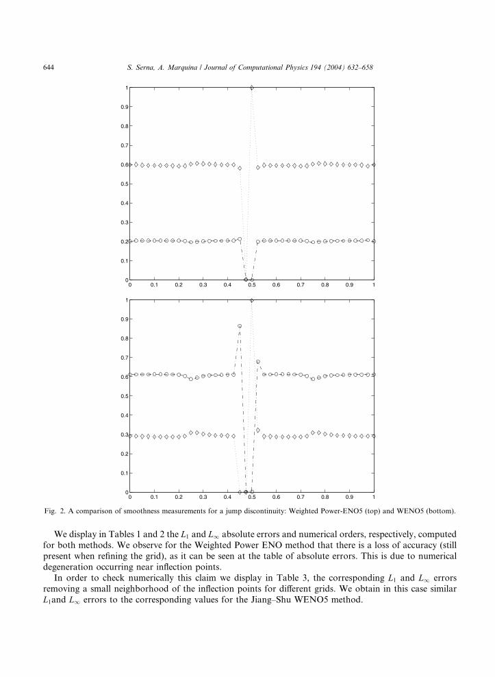
Fig. 2. A comparison of smoothness measurements for a jump discontinuity: Weighted Power-ENO5 (top) and WENO5 (bottom).


We display in Tables 1 and 2 the L1 and L1 absolute errors and numerical orders, respectively, computed

for both methods. We observe for the Weighted Power ENO method that there is a loss of accuracy (still

present when refining the grid), as it can be seen at the table of absolute errors. This is due to numerical

degeneration occurring near inflection points.

In order to check numerically this claim we display in Table 3, the corresponding L1 and L1 errors

removing a small neighborhood of the inflection points for different grids. We obtain in this case similar

L1and L1 errors to the corresponding values for the Jiang–Shu WENO5 method.

Fig. 3. A comparison of smoothness measurements for two discontinuities in derivative: Weighted Power-ENO5 (top) and WENO5

(bottom).


5. Numerical experiments

We start our calculations with the linear advection of signals. We will consider the following

problems:

Table 2

Numerical orders for Weighted Power-ENO5 and WENO5 methods

N L1-order L1-order

WPower-ENO5 WENO5 WPower-ENO5 WENO5

160 – – – –

320 4.22 4.99 3.86 5.04

640 4.97 4.99 4.46 5.08

1280 4.80 5.01 4.68 5.04

Table 1

Absolute errors for Weighted Power ENO5 and WENO5 methods

N L1-error L1-error

Weighted Power-ENO5 WENO5 WPower-ENO5 WENO5

80 1:75� 10�5 7:17� 10�7 1:53� 10�4 1:37� 10�6

160 9:40� 10�7 2:24� 10�8 9:58� 10�6 4:18� 10�8

320 3:09� 10�8 7:08� 10�10 6:27� 10�7 1:23� 10�9

640 1:40� 10�9 2:29� 10�11 6:86� 10�8 4:02� 10�11

1280 5:01� 10�11 7:03� 10�13 2:67� 10�9 1:06� 10�12

Table 3

Absolute errors for Weighted Power ENO5 and WENO5, excluding inflection points

N L1-error L1-error

WPower-ENO5 WENO5 WPower-ENO5 WENO5

80 4:17� 10�6 8:76� 10�7 1:62� 10�5 1:35� 10�6

160 9:85� 10�8 2:72� 10�8 6:88� 10�7 4:18� 10�8

320 2:00� 10�10 8:27� 10�10 9:84� 10�10 1:23� 10�9

640 6:89� 10�12 2:46� 10�11 4:81� 10�11 4:01� 10�11


5.1. Example 1: Linear advection

We solve the linear equation

ut þ ux ¼ 0; a6 x6 b;

with uðx; 0Þ ¼ u0ðxÞ periodic in ½a; b�, for the cases:

5.1.1. Example 1.1

½a; b� ¼ ½0; 1� and

u0ðxÞ ¼1; 0:356 x6 0:65;0; otherwise:

�

5.1.2. Example 1.2

½a; b� ¼ ½�1; 1� and

u0ðxÞ ¼ sin p xþ0:30:6

; �0:36 x6 0:3;

0; otherwise:

�


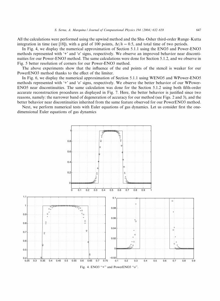
All the calculations were performed using the upwind method and the Shu–Osher third-order Runge–Kutta

integration in time (see [18]), with a grid of 100 points, Dt=h ¼ 0:5, and total time of two periods.

In Fig. 4, we display the numerical approximation of Section 5.1.1 using the ENO3 and Power-ENO3methods represented with �+� and �o� signs, respectively. We observe an improved behavior near disconti-

nuities for our Power-ENO3 method. The same calculations were done for Section 5.1.2, and we observe in

Fig. 5 better resolution of corners for our Power-ENO3 method.

The above experiments show that the influence of the end points of the stencil is weaker for our

PowerENO3 method thanks to the effect of the limiter.

In Fig. 6, we display the numerical approximation of Section 5.1.1 using WENO5 and WPower-ENO5

methods represented with �+� and �o� signs, respectively. We observe the better behavior of our WPower-

ENO5 near discontinuities. The same calculation was done for the Section 5.1.2 using both fifth-orderaccurate reconstruction procedures as displayed in Fig. 7. Here, the better behavior is justified since two

reasons, namely: the narrower band of degeneration of accuracy for our method (see Figs. 2 and 3), and the

better behavior near discontinuities inherited from the same feature observed for our PowerENO3 method.

Next, we perform numerical tests with Euler equations of gas dynamics. Let us consider first the one-

dimensional Euler equations of gas dynamics

Fig. 4. ENO3 ‘‘+’’ and PowerENO3 ‘‘o’’.

Fig. 5. ENO3 ‘‘+’’ and PowerENO3 ‘‘o’’.

Fig. 6. WENO5 ‘‘+’’ and WPower-ENO5 ‘‘o’’.


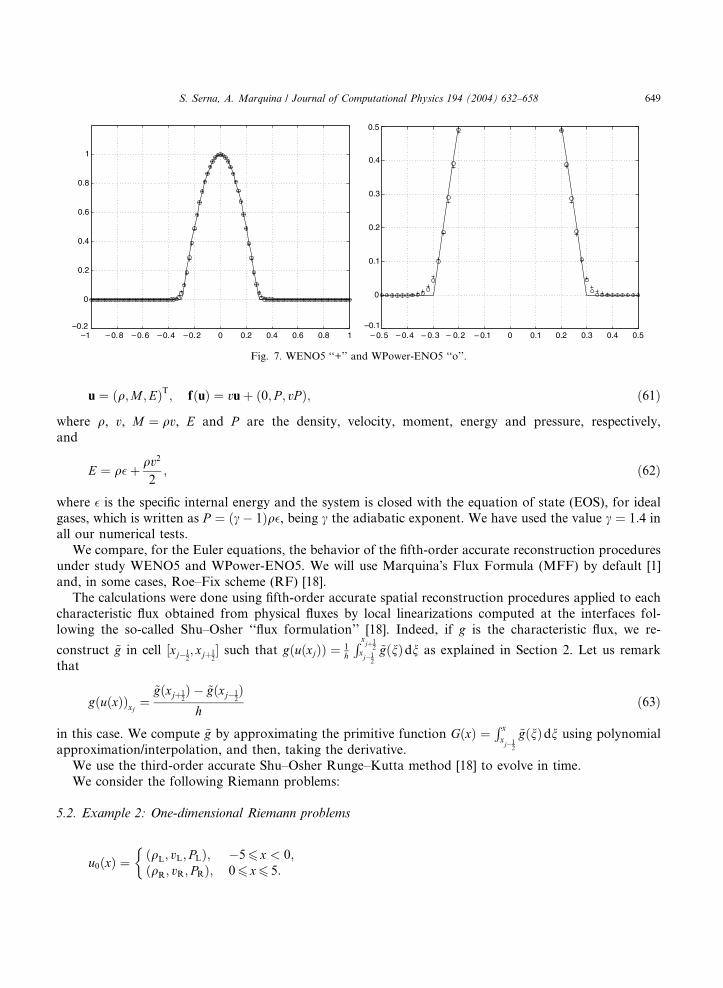
Fig. 7. WENO5 ‘‘+’’ and WPower-ENO5 ‘‘o’’.


u ¼ ðq;M ;EÞT; fðuÞ ¼ vuþ ð0; P ; vP Þ; ð61Þ

where q, v, M ¼ qv, E and P are the density, velocity, moment, energy and pressure, respectively,

and

E ¼ q�þ qv2

2; ð62Þ

where � is the specific internal energy and the system is closed with the equation of state (EOS), for ideal

gases, which is written as P ¼ ðc� 1Þq�, being c the adiabatic exponent. We have used the value c ¼ 1:4 inall our numerical tests.

We compare, for the Euler equations, the behavior of the fifth-order accurate reconstruction procedures

under study WENO5 and WPower-ENO5. We will use Marquina�s Flux Formula (MFF) by default [1]

and, in some cases, Roe–Fix scheme (RF) [18].

The calculations were done using fifth-order accurate spatial reconstruction procedures applied to each

characteristic flux obtained from physical fluxes by local linearizations computed at the interfaces fol-

lowing the so-called Shu–Osher ‘‘flux formulation’’ [18]. Indeed, if g is the characteristic flux, we re-

construct ~g in cell ½xj�12; xjþ1

2� such that gðuðxjÞÞ ¼ 1

h

R xjþ1

2xj�1

2

~gðnÞdn as explained in Section 2. Let us remark

that

gðuðxÞÞxj ¼~gðxjþ1

2Þ � ~gðxj�1

2Þ

hð63Þ

in this case. We compute ~g by approximating the primitive function GðxÞ ¼R xxj�1

2

~gðnÞdn using polynomial

approximation/interpolation, and then, taking the derivative.

We use the third-order accurate Shu–Osher Runge–Kutta method [18] to evolve in time.

We consider the following Riemann problems:

5.2. Example 2: One-dimensional Riemann problems

u0ðxÞ ¼ðqL; vL; PLÞ; �56 x < 0;ðqR; vR; PRÞ; 06 x6 5:

�

Fig. 8. WENO5-MFF ‘‘+’’ and WPower-ENO5-MFF ‘‘o’’.

Fig. 9. WENO5-MFF ‘‘+’’ and WPower-ENO5-MFF ‘‘o’’.


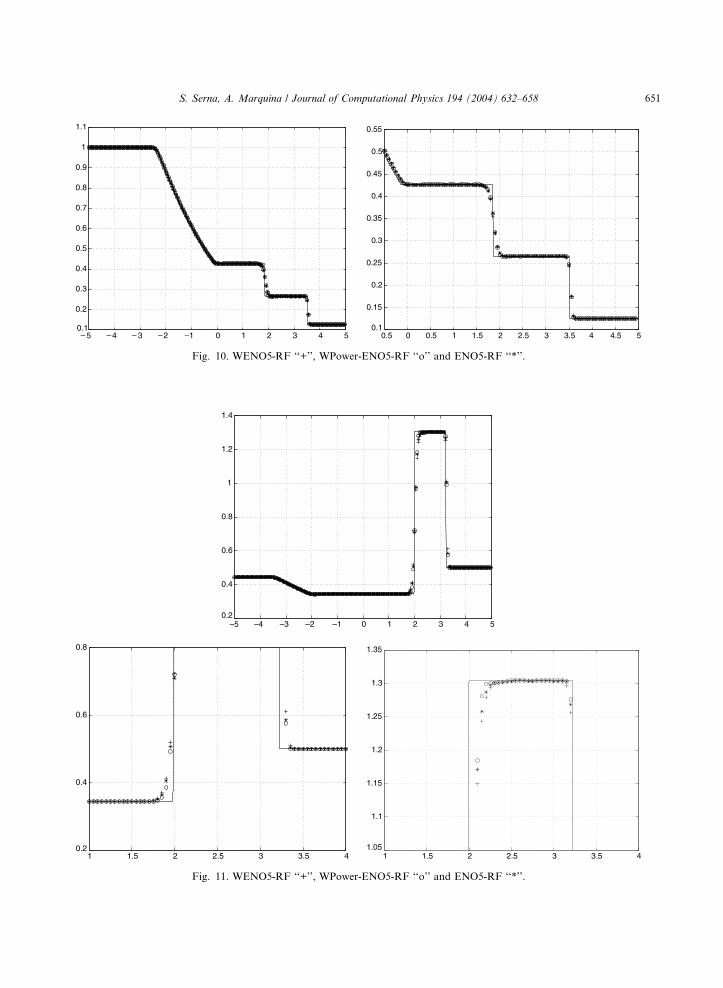
Fig. 10. WENO5-RF ‘‘+’’, WPower-ENO5-RF ‘‘o’’ and ENO5-RF ‘‘*’’.

Fig. 11. WENO5-RF ‘‘+’’, WPower-ENO5-RF ‘‘o’’ and ENO5-RF ‘‘*’’.



5.2.1. The Sod’s problem [19]

ðqL; vL; PLÞ ¼ ð1; 1; 1Þ;

ðqR; vR; PRÞ ¼ ð0:125; 0; 0:1Þ:

5.2.2. Lax’s problem [6]

ðqL; vL; PLÞ ¼ ð0:445; 0:698; 3:528Þ;

ðqR; vR; PRÞ ¼ ð0:5; 0; 0:571Þ:

The computations for both cases were done using 200 equal spaced grid points with a constant ratio

Dt=h ¼ 0:2 until time 2 for the Sod�s Tube and Dt=h ¼ 0:1 until time 1.3 for the Lax�s Tube. The solid lines

represent the exact solution evaluated in 5000 points, see [16].

Fig. 12. zoomed regions of density profile, WENO5 ‘‘+’’, WPower-ENO5 and ‘‘o’’.


In Figs. 8 and 9, we display the numerical results of the density profile. The better behavior near dis-

continuities for our WPower-ENO5 method is more conspicuous for the Lax�s Tube experiment (see

zoomed regions at the bottom of Fig. 9).In order to appreciate the behavior of the fifth-order Weighted ENO reconstruction methods with re-

spect to the classical fifth-order ENO method, we have also computed both Riemann problems using Roe–

Fix scheme. Indeed, we have implemented WENO5-RF, WPower-ENO5-RF and the classical ENO5-RF

schemes using the Shu–Osher flux formulation.

In Figs. 10 and 11, we observe that WPower-ENO5-RF scheme resolves better the contact discontinuity

than ENO5-RF and WENO5-RF schemes.

In what follows, we only use Marquina�s Flux Formula as approximate Riemann solver.

5.3. Example 3: One-dimensional shock entropy wave interaction

Next, we consider a moving Mach 3 shock interacting with sine waves in density, used as a benchmark inShu–Osher ([18], see also [12]).

Fig. 13. WENO5 left pictures with 400 and 800 points, WPower-ENO5 right pictures with 400 and 800 points.


We consider the initial data:

u0ðxÞ ¼ðqL; vL; PLÞ; �56 x < �4;ðqR; vR; PRÞ; �46 x6 5

�

ðqL; vL; PLÞ ¼ ð3:85714; 2:62936; 10:33333Þ and ðqR; vR; PRÞ ¼ ð1þ 0:2 sinð5xÞ; 0; 1Þ.The numerical results of the density profile are displayed in Fig. 12. Solid line correspond to the nu-

merical solution by WENO5 with 1600 points, that can be seen as the ‘‘exact’’ solution. We compute thenumerical approximation for 400 points at time¼ 1.8 and Dt=h ¼ 0:1 for WENO5 and WPower-ENO5, �+�and �o� signs, respectively. We observe in Fig. 12 that fine structure in the density profile makes our

WPower-ENO5 method to perform better than the WENO5 one. This feature is a consequence of the fact

that the WPower-ENO5 method is more compressive (it produces more total variation in cell) than

WENO5 method. On the other hand, we observe again a reduced smearing near shocks (see zoomed re-

gions at the bottom of Fig. 12).

Fig. 14. WENO5 (left), WPower-ENO5 (right).


5.4. Example 4: Two interacting blast waves

This experiment was originally proposed as a benchmark by Woodward and Colella [20]

u0ðxÞ ¼ðqL; vL; PLÞ; 06 x < 0:1;ðqM; vM; PMÞ; 0:16 x < 0:9;ðqR; vR; PRÞ; 0:96 x6 1:

8<:

ðqL; vL; PLÞ ¼ ð1; 0; 103Þ, ðqM; vM; PMÞ ¼ ð1; 0; 10�2Þ and ðqR; vR; PRÞ ¼ ð1; 0; 102Þ.We display in Fig. 13 the density component computed with 400 and 800 grid points (top and bottom,

respectively). We evolved until time 0.038 with Dt=h ¼ 0:01 for WENO5 (left) and WPower-ENO5 (right).We observe that the local extrema are better resolved for our WPower-ENO5 method. We did com-

putations with different number of grid points and we observe good convergence rate to the ‘‘exact’’ so-

lution (computed by WENO5 with 2000 points).

Finally, we will present two numerical experiments for the two-dimensional Euler equations for gas

dynamics.

0 0.1 0.2 0.3 0.4 0.5 0.6 0.7 0.8 0.9 10.2

0.4

0.6

0.8

1

1.2

1.4

1.6

1.8

0.4

0.6

0.8

1

1.2

1.4

0.4

0.5

0.6

0.7

0.8

0.9

1

1.1

1.2

1.3

Fig. 15. Top, section of density profile at x ¼ 0:2575. Bottom, zoomed regions of the x-section. WENO5 ‘‘+’’ and WPower-ENO5 ‘‘o’’.

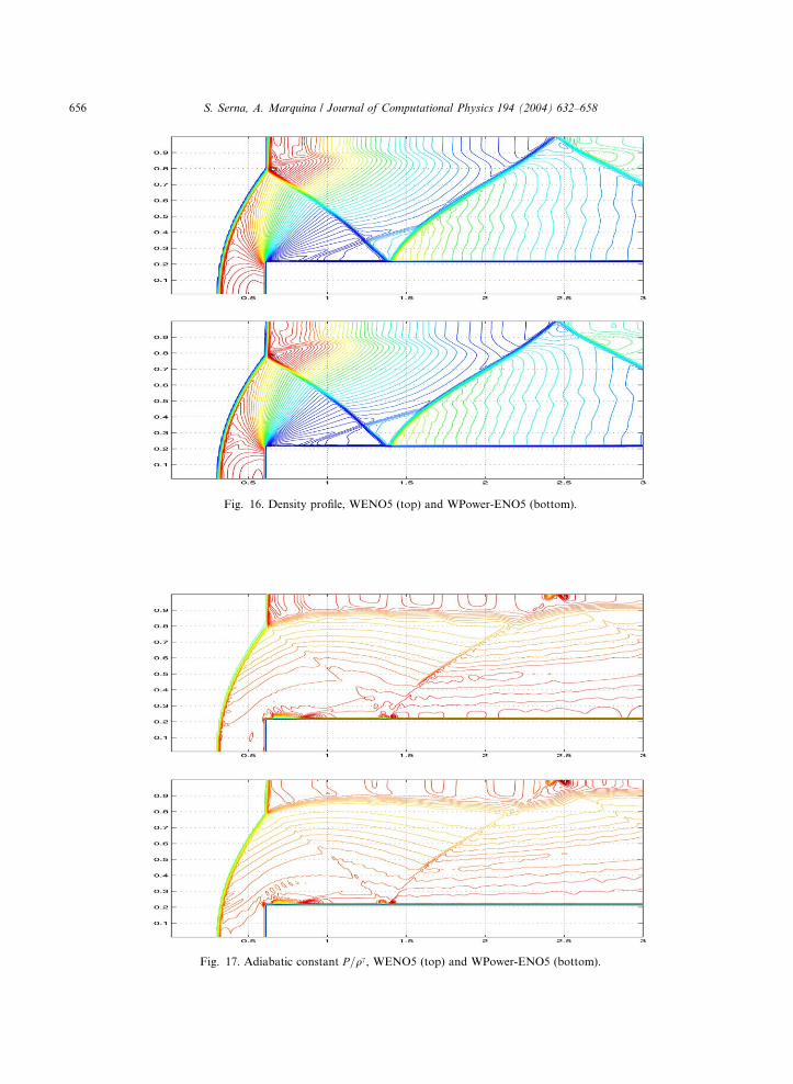
Fig. 16. Density profile, WENO5 (top) and WPower-ENO5 (bottom).

Fig. 17. Adiabatic constant P=qc, WENO5 (top) and WPower-ENO5 (bottom).


0

1

2

3

4

5

0.5

1

1.5

2

2.5

3

3.5

4

4.5

5

Fig. 18. Sections of density profile at x ¼ 0:8 (left) and y ¼ 0:5 (right), WENO5 �+� and WPower-ENO5 �o�.


5.5. Example 5: Two-dimensional Riemann problem

A two-dimensional Riemman problem consists in an initial data defined as constants states on each of

the four quadrants. We consider the four contacts Riemann problem defined in [15] and we evolve this

initial data until time 1.6, with a CFL factor of 0.8 for a grid of 400� 400 points for WENO5 and WPower-

ENO5 methods. We observe a better resolved vortex at the top for our WPower-ENO5 method at Fig. 14.

Also, we displayed at Fig. 15 a x-section, that traverses the vortex, showing the better resolution of thecontact discontinuities of our WPower-ENO5 method versus WENO5 method (see the fine structure of the

vortex region at the bottom of the figure).

5.6. Example 6: Mach 3 wind tunnel with a step

This test problem, introduced by Emery [2], has been carefully analyzed in [1,20]. The problem is ini-

tialized by a uniformMach 3 flow in a tunnel containing a step. The tunnel is 1 length unit wide and 3 length

units long. The step is 0.2 length units high and is located 0.6 units from the left-hand end of the tunnel.

Inflow boundary conditions are applied at the left-hand end and outflow boundary conditions are ap-

plied at the right-hand end of the computational domain. Reflective boundary conditions are applied along

the walls of the tunnel. We use at the corner of the step the boundary entropy and enthalpy correctionsdiscussed in detail in [1]. We use this example to test the robustness of our method in presence of reflective

boundary conditions.

We evolve the initial data until time 4 for a grid of 240� 80 grid points with a CFL factor of 0.8 . We

display the contour lines of the density profiles in Fig. 16, and the adiabatic constant profiles in Fig. 17. We

observe good resolution and location of the strong reflective waves appearing in this test and we have

slightly better resolution at the contact line for our scheme.

In Fig. 18, we display sections of the density component. The left picture is the x-section at x ¼ 0:8,where we observe better resolution of the weak contact for our WPower-ENO5 method.

6. Conclusions

We have introduced an extended class of limiters that includes the ENO limiters as particular case. These

limiters are used to design total variation stable polynomial reconstructions when applied to second-order


differences. In this paper, we have proposed a new weighted ENO method, based on the extended limiters,

that reaches optimal accuracy on smooth regions and improves the behavior of WENO methods near

discontinuities. We presented several one- and two-dimensional numerical experiments for scalar andsystems of conservation laws to show the evidence of the above features.

We remark that in numerical experiments where fine structures appear to be important (e.g., vortex

regions), the Weighted Power ENO method shows substantial improvements in resolving fine scales, in

spite of the improvements observed in standard numerical tests might seem to be minor.

References

[1] R. Donat, A. Marquina, Capturing shock reflections: an improved flux formula, J. Comput. Phys. 125 (1996) 42–58.

[2] A.F. Emery, J. Comput. Phys. 2 (1968) 306.

[3] A. Harten, High resolution schemes for hyperbolic conservation laws, J. Comput. Phys. 49 (1983) 357–393.

[4] A. Harten, B. Engquist, S. Osher, S. Chakravarthy, Uniformly high order accurate essentially non-oscillatory schemes III, J.

Comput. Phys. 71 (2) (1987) 231–303.

[5] G.S. Jiang, C.W. Shu, Efficient Implementation of weighted ENO schemes, J. Comput. Phys. 126 (1996) 202–228.

[6] P.D. Lax, Weak solutions of nonlinear hyperbolic equations and their numerical computation, Commun. Pure Appl. Math. 7

(1954) 159–193.

[7] S. Li, L. Petzold, Moving mesh methods with upwinding schemes for time-dependent PDEs, J. Comput. Phys. 131 (1997) 368–377.

[8] R.J. LeVeque, Numerical Methods for Conservation Laws, Birkhauser Verlag, Zuerich, 1990.

[9] X-D. Liu, S. Osher, T. Chan, Weighted essentially non-oscillatory schemes, J. Comput. Phys. 115 (1994) 200–212.

[10] A. Marquina, Local piecewise hyperbolic reconstructions for nonlinear scalar conservation laws, SIAM J. Sci. Comput. 15 (1994)

892–915.

[11] A. Marquina, S. Serna, Afternotes on PHM: harmonic ENO methods, in: Proceedings of the Ninth International Conference on

Hyperbolic Problems: Theory, Numerics, Applications, HYP2002, Caltech, Pasadena, CA, Springer, 2002.

[12] J. McKenzie, K. Westphal, Interaction of linear waves with oblique shock waves, Phys. Fluids 11 (1968) 2350–2362.

[13] S.J. Osher, S. Chakravarty, High resolution schemes and the entropy condition, SIAM J. Numer. Anal. 21 (1984) 955–984.

[14] A. Rogertson, E. Meiburg, A numerical study of the convergence of ENO schemes, J. Sci. Comput. 5 (1990) 151–167.

[15] C.W. Schulz-Rinne, J.P. Collins, H.M. Glaz, Numerical solution of the Riemann problem for two-dimensional gas dynamics,

SIAM J. Sci. Comput. 14 (1993) 1394–1414.

[16] J. Smoller, Shock Waves and Reaction–Diffusion Equations, Springer Verlag, New York, 1983.

[17] C.W. Shu, Numerical experiments on the accuracy, J. Sci. Comput. 5 (1990) 127–150.

[18] C.W. Shu, S.J. Osher, Efficient implementation of essentially non-oscillatory shock capturing schemes II, J. Comput. Phys. 83

(1989) 32–78.

[19] G. Sod, A survey of several finite difference methods for systems of nonlinear hyperbolic conservation laws, J. Comput. Phys. 27

(1978) 1–31.

[20] P. Woodward, P. Colella, The numerical simulation of two-dimensional fluid flow with strong shocks, J. Comput. Phys. 54 (1984)

115–173.

Power ENO methods: a ﬁfth-order accurate Weighted Power ...

Documents

Transcript of Power ENO methods: a ﬁfth-order accurate Weighted Power ...