POVERTY ESCAPE ROUTES IN CENTRAL TANZANIA: COPING ...
50
Transcript of POVERTY ESCAPE ROUTES IN CENTRAL TANZANIA: COPING ...


ii
POVERTY ESCAPE ROUTES IN CENTRAL TANZANIA: COPING STRATEGIES IN
SINGIDA AND DODOMA REGIONS
VOL. I
By
Dr. Flora Kessy
Dr. Oswald Mashindano
Mr. Dennis Rweyemamu
Mr. Prosper Charle
ESRF Discussion Paper No. 38
PUBLISHED BY: The Economic and Social Research Foundation (ESRF)
51 Uporoto Street (Off Ali Hassan Mwinyi Road), Ursino Estate
P.O. Box 31226
Dar es Salaam, Tanzania.
Tel: (+255) 22 2760260, 2760751/52
Mobile: (+255) 754 280133
Fax: (+255) 22 2760062
Email: [email protected]
Website: www.esrftz.org
ISBN 978-9987-610-68-6
© 2011 Economic and Social Research Foundation

iii
TABLE OF CONTENTS
TABLE OF CONTENTS ................................................................................................................... III
LIST OF TABLES ............................................................................................................................ V
LIST OF ACRONYMS ..................................................................................................................... VI
ABSTRACT .................................................................................................................................... 1
1.0 INTRODUCTION ................................................................................................................. 2
1.1 BACKGROUND TO THE STUDY .......................................................................................................... 2
1.2 GROWTH AND POVERTY STATUS IN SINGIDA REGION .......................................................................... 3
1.2.1 Growth and non-income indicators ................................................................................... 3
1.2.2 Assessment by Human Development Index and Human Poverty Index ............................ 3
1.2.3 Combining Household Budget Survey Data with Census Information .............................. 4
1.2.4 Assessment by District Level Poverty Estimates ................................................................ 5
1.3 OBJECTIVES OF THE STUDY .............................................................................................................. 6
1.4 RESEARCH QUESTIONS ................................................................................................................... 7
2.0. METHODOLOGY ................................................................................................................. 8
2.1 QUALITATIVE METHODS ................................................................................................................. 8
2.2 THE QUANTITATIVE SURVEY .......................................................................................................... 10
2.3 SAMPLING FRAME ....................................................................................................................... 10
2.4 PROFILES OF THE SAMPLED COMMUNITIES ...................................................................................... 10
2.4.1 Muhalala Community ...................................................................................................... 10
2.4.2 Makale Community ......................................................................................................... 11
2.4.3 Kidarafa Community ....................................................................................................... 11
2.4.4 Kinalilya Community ........................................................................................................ 11
3.0 DATA ANALYSIS ............................................................................................................... 13
3.1 QUALITATIVE ANALYSIS ................................................................................................................ 13
3.2 QUANTITATIVE ANALYSIS .............................................................................................................. 13
3.2.1 Descriptive Statistics........................................................................................................ 13
3.2.2 Descriptive Statistics of the Variables Used in the Analyses ........................................... 13
3.3 TRIANGULATING QUALITATIVE WITH QUANTITATIVE DATA ................................................ 14
3.4 REGRESSION ANALYSIS MODELS .................................................................................................... 15
3.5 TRIANGULATING THE REGRESSION RESULTS WITH QUALITATIVE INFORMATION ..................................... 16
4.0 COMMUNITY AND HOUSEHOLD FACTORS AFFECTING MOBILITY ....................................... 20
4.1 CHANGES IN INCOME OPPORTUNITIES ............................................................................................ 20
4.2 AGRICULTURE AND LIVESTOCK DEVELOPMENT ................................................................................. 20
4.3 HOUSEHOLD MOBILITY: THE LADDER OF LIFE................................................................................... 21
4.3.1 Downward Movement to Chronic Poverty ...................................................................... 22
5.0 FACTORS FOR UPWARD MOVEMENT (POVERTY ESCAPE ROUTES) ..................................... 24
5.1 GOVERNANCE AND MOBILITY ........................................................................................................ 24
5.2 PUBLIC SOCIO-ECONOMIC SERVICES AND MOBILITY.......................................................................... 27
5.2.1 Un-met Needs to Access to Services ................................................................................ 28

iv
5.2.2 Adequacy and Reliability of Services ............................................................................... 29
5.2.3 Key Players of Service Providers ...................................................................................... 29
5.2.4 Community Participation in Services ............................................................................... 30
6.0 CONCLUSIONS AND POLICY IMPLICATIONS ....................................................................... 32
REFERENCES .............................................................................................................................. 33
ESRF PUBLICATIONS ................................................................................................................... 34
APPENDIX I: DETAILS OF REGRESSION RESULTS FOR VOL. I & II ................................................ 38

v
LIST OF TABLES
Table 1: Non Income Indicators based on 2000/01 Household Budget Survey ....................... 3
Table 2: Percent of Households below Poverty Line ................................................................... 4
Table 3: Selected Poverty Estimates at District Level .................................................................. 5
Table 4: Major Crops Grown in Singida Region ........................................................................ 20

vi
LIST OF ACRONYMS
AFNET Anti-Female Genital Mutilation Network
AMSDP Agricultural Marketing System Development Program
ATTT Association of Tanzania Tobacco Traders
BCU Biharamulo Cooperative Union
CBOs Community Based Organizations
CSOs Civil Service Organizations
FGD Focus Group Discussion
HBS Household Budget Survey
HDI Human Development Index
HIPC Highly Indebted Poor Countries
HPI Human Poverty Index
ITI International Trachoma Initiative
KCU Kagera Cooperative Union
KDCU Karagwe Development Cooperative Union
MBICU Mbinga Cooperative Union
MCH Maternal and Child Health
MDGs Millennium Development Goals
MMA Mixed Method Approach
NACP National AIDS Control Program
NPES National Poverty Eradication Strategy
NSGRP National Strategy for Growth and Reduction of Poverty
OLS Ordinary Least Square
PEDP Primary Education Development Plan
PLHA People Living with HIV/AIDS
PRSP Poverty Reduction Strategy Paper
SACCOS Savings and Credit Cooperative Societies
SAFE Surgery, Antibiotics, Facial Cleanliness and Environment
TASAF Tanzania Social Action Fund
TCRS Tanzania Christian Refugees Services
THIS Tanzania HIV Indicators Survey
TLTC Tanzania Leaf Tobacco Company
TzPPA Tanzania Participatory Poverty Assessment
TZS Tanzania Shillings
URT United Republic of Tanzania
VEO Village Executive Officer

1
ABSTRACT
This report is organized in three volumes as follows: Volumes I and II examines Poverty Escape
Routes and Factors Affecting Mobility in Singida and Dodoma regions respectively, whereas Volume
III focuses on the Coping Strategies used in Singida and Dodoma regions. The series provide an
overview of poverty status in the respective regions, objectives of the study, the methodology used in
carrying out the study, including the data collection and analysis techniques. The findings of this
study focus on Singida region and are divided into community and household factors affecting
mobility.
Data on these volumes complement each other in the final analysis and therefore the conclusions and
policy implications are combined and should be read in conjunction to reflect a comprehensive picture
of poverty escape routes in the Central Zone of Tanzania. Conclusion and policy recommendations
provided accentuate the importance of agriculture for both income and food poverty escape routes as it
was observed that households in the study area rely on planting of sunflower, groundnuts, and
tobacco as cash crops and maize, millet, sorghum, and cassava as main food crops. Production of cash
crops that have reliable market such as tobacco contributes to households’ upward mobility. On the
other hand, the role of the private sector in providing agricultural inputs, extension services, and
reliable market for cash crops has been vividly portrayed as the perfect poverty escape route. In
addition, formal organizations such as Primary Cooperative Societies are instrumental in providing
loans for investing in agriculture.

2
1.0 INTRODUCTION
1.1 Background to the Study
Since independence in 1961, the Government of Tanzania has been preoccupied with
combating poverty. National efforts to tackle the problem were initially channeled through
centrally directed, medium-term and long-term development plans, and resulted in a
significant improvement in per capita income and access to education, health and other
social services until 1970s. Thereafter, these gains could not be sustained because of various
domestic and external shocks, and policy weaknesses.
After a decade of preoccupation with re-establishing macro-economic stability and
structural reforms aimed at creating an enabling environment, Tanzania has resumed its
focus on poverty reduction. This renewal is part of a global effort for a sustained exit from
the poverty trap. The Government has been undertaking various initiatives towards poverty
reduction and attainment of social and economic development. Those efforts are found
within a broad policy framework, the Tanzania Development Vision 2025, which stipulates
the vision, mission, goals and targets to be achieved with respect to economic growth and
poverty eradication by the year 2025. As an effort to operationalize the Tanzania
Development Vision 2025, the Government formulated the National Poverty Eradication
Strategy (NPES), which provides overall guidance to all stakeholders and provides a
framework for co-ordination and supervision of the implementation of policies and
strategies of poverty eradication.
The Poverty Reduction Strategy Paper (PRSP) was thereafter formulated as a Medium-Term
Strategy of poverty reduction, in the context of the enhanced Highly Indebted Poor
Countries (HIPC) initiative. Initially, the country implemented a three year PRS I, (2000/01 –
2003/04). Thereafter, the Government approved the PRS II popular by the name of
MKUKUTA (National Strategy for Growth and Reduction of Poverty - NSGRP) in early
2005. The NSGRP keeps in focus the aspirations of Tanzania’s Development Vision 2025 for
high quality livelihood, good governance and rule of law, strong and competitive economy.
It is committed to the Millennium Development Goals (MDGs), as internationally agreed
targets for reducing poverty, hunger, diseases, illiteracy, environmental degradation and
discrimination against women by 2015.
The implementation of NSGRP and the broader Vision 2025 at the lower level is done across
sectors and regions, and districts. It is within this context that the Economic and Social
Research Foundation (ESRF) in 2005/06 conducted a study on poverty escape routes in
Central Tanzania which aimed at soliciting data and information on factors for upward and
downward mobility of different households and individuals in Singida region. The study
has strong relevance for policy design and monitoring of poverty reduction strategies and
policies in Tanzania because, it provides policy insights based on the experiences of those

3
who have actually moved out of poverty and stayed out of poverty over time, those who
have maintained their wealth over time, and those who have fallen down and / or stayed
trapped in chronic poverty. The study focuses on a wide range of social, political,
institutional and economic mechanisms that hinder or facilitate poor people’s access to
economic opportunities and movement out of poverty.
1.2 Growth and Poverty Status in Singida Region
1.2.1 Growth and non-income indicators
Since late 1990s, Singida region has been experiencing positive per capita income growth.
Data from the National Bureau of Statistics show that, in early 20th century, Singida region
experienced per capita income growth of about 8 percent. However, the recorded growth
has not adequately translated into improved wellbeing, as indicated by the information from
the Household Budget Survey (HBS) (Table 1). In comparison with other regions, the non-
income indicators reveal a mixed picture as quite a number of them show that Singida
region is relatively performing better than other regions, while other indicators show
otherwise.
Table 1: Non Income Indicators based on 2000/01 Household Budget Survey
Indicator Dodoma Singida DSM Rukwa Arusha Lindi
% of Adults without education 31 27 8 30 20 44
% of Household using piped or protected source
of drinking water
65
61
94
55
59
24
% of Households within 1 km of drinking water
in the dry season
49
51
84
63
49
47
% of Households within 2 km of primary school
49
56
81
75
54
79
% of Households within 6 km of dispensary
and/or health center
49
82
98
82
73
68
% of Individuals below the food poverty line
13
27
8
19
25
33
% of Individuals below the basic needs poverty
line
34
55
18
31
39
53
Source URT (2002)
1.2.2 Assessment by Human Development Index and Human Poverty Index1
The 2005 Poverty and Human Development Report classified the Tanzania regions
according to their performance based on Human Development Index (HDI) and Human
Poverty Index (HPI). The report groups the regions into three categories: High HDI regions,
Medium HDI regions, and Low HDI regions. The Report shows that 5 regions with High
1The Human Development Index (HDI) is a summary measure of human development using the average
achievements in three basic dimensions of Human Development namely (1) Long and Healthy life (measured by
life expectance at birth); (2) Knowledge (Measured by literacy rate) and (3) Decent Standard of Living (Measured
by per capita income). On the other hand, Human Poverty Index (HPI) measures the extent of human poverty as
portrayed by lack of these three dimensions of human development, i.e., lack of long and healthy life, lack of
knowledge, and lack of decent standard of living.

4
Human Development Index as Dar es Salaam (0.746), Kilimanjaro (0.620), Arusha (0.555),
Mbeya (0.551), and Iringa (0.524). The medium Human Development Index category is
occupied by ten regions, while 5 regions are classified under Low Human Development
Index. Singida is categorized under Medium Human Development Index (0.483)
performing much better than Dodoma (0.432), however, both Singida has HDI below the
average for Mainland Tanzania index of (0.495).
On the other hand, the HPI shows that 5 regions namely Dar es Salaam (7.9), Kilimanjaro
(12.4), Mbeya (14.8), Ruvuma (18.2) and Morogoro (19.2) are best performers, followed by 10
regions with Medium Human Poverty Index, while 5 regions are classified as worst
performers. Singida region is classified under the Medium Human Poverty Index of (21.3)
performing much better than Dodoma (22.9). Again, the HPI values for Singida are worse
than the average HPI for Mainland Tanzania (22.1).
1.2.3 Combining Household Budget Survey Data with Census Information
The 2005 Poverty and Human Development Report combined the 2001 Household Budget
Survey with the 2002 Census data to derive new regional poverty estimates with much
smaller standard errors (Table 2). The derived estimates of regional poverty were more
precise than the previously available estimates. As indicated in table 2 below, Singida ranks
second as the most deprived region out of the then 20 mainland regions.
Table 2: Percent of Households below Poverty Line
Sn Region Percent of Households Below Poverty Line Rank2
1 Kagera 29 11
2 Kigoma 38 6
3 Singida 49 2
4 Dodoma 32 9
5 Kilimanjaro 28 12
6 Tanga 26 13
7 Mara 50 1
8 Coast 38 6
9 Morogoro 28 12
10 Mtwara 38 6
11 Lindi 39 5
12 Mbeya 23 14
13 Tabora 40 4
14 Mwanza 43 3
15 Shinyanga 43 3
16 Ruvuma 37 7
17 Iringa 28 12
18 Arusha 21 15
19 Rukwa 36 4
20 Dar es Salaam 19 16
Source: URT, (2005).
2 Rank 1 depicts the most deprived region

5
1.2.4 Assessment by District Level Poverty Estimates
Using the poverty mapping techniques, it has been possible to estimate poverty at district
level. Because districts are smaller, and with corresponding smaller sample sizes than
regions, standards errors are higher but, in more than 90 percent of the cases, standard
errors of the resulting district estimates were below the standard errors of the HBS’s regional
estimates (URT, 2005). Table 3 shows selected indicators in Singida districts, together with
Mara (worst values category) and Arusha (best values category). For most of the indicators,
the districts in Singida region are moderate performers.
Table 3: Selected Poverty Estimates at District Level
District
Populatio
n per
health
facility
(2002)
Primary
Net
Enrolment
(2004)
Primary
Pupil-
Class
Ratio
(2004)
% of HH
using
Piped or
Protected
Water
Source
(2002)
% of
HH
Owning
a Radio
(2002)
% of
HH
Owning
a
Bicycle
(2002)
Infant
Mortality
Rate (per
1,000 live
births)
(2002)
Under
five
Mortality
Rate (per
1,000 live
births)
(2002)
Singida
Iramba 7647 82 76 30 34 31 79 125
Singida (R) 9100 85 105 39 31 26 79 126
Manyoni 5527 82 76 36 44 28 100 165
Singida (U) 6756 98 87 61 39 23 69 108
Dodoma
Kondoa 7381 88 72 39 45 31 70 110
Mpwapwa 6340 79 78 65 39 19 128 217
Kongwa 9209 72 87 74 49 39 116 195
Dodoma (R) 6095 66 68 51 31 22 142 299
Dodoma (U) 5869 75 88 64 60 32 94 153
Mara
Tarime 9088 100 80 22 45 35 123 207
Serengeti 5502 - 74 47 45 36 109 181
Musoma (R) 7329 100 100 17 52 44 115 191
Bunda 8929 100 77 51 61 44 102 166
Musoma (U) 4148 100 - 92 64 41 84 134
Arusha
Monduli 4393 71 66 49 35 15 35 48
Arumeru 7352 99 75 85 70 24 41 58
Arusha (U) 4542 93 87 99 79 19 39 55
Karatu 5932 100 69 64 44 27 61 93
Ngorongoro 7187 71 77 34 76 3 31 40
Source: URT, (2005).
However, the assessment of this region using individual indicators reveals that poverty is
still prevalent. The review of available data also suggests that some areas within the Central
Tanzania have experienced growth without a commensurate reduction in poverty, which
implies that pockets of poverty persist. This is a typical scenario observed at national level;

6
where the change in economic growth since the 1990s hasn’t proportionally been translated
into poverty reduction.
Two important lessons can therefore be drawn: Firstly, there is a notable evidence of
mismatch between economic growth and grassroots changes in welfare and overall living
standards, judging from individual indicators of growth and poverty. While economic
growth has been positive over time, performance of most of the welfare indicators in the
region does not support this trend. It is therefore important to understand the reasons and
factors behind this puzzle. It is possible that while growth is evident, equity is not
guaranteed due to inefficient system and lack of infrastructure for distribution. It is also
possible that the findings are premised on weak methodologies, which omit non-income
variables. This drives the study objectives underneath.
1.3 Objectives of the Study
This study aimed at deepening the understanding of the key characteristics of the poor in
Singida region and the changes in the conditions and characteristics of poverty and income
generation. Also, the study sheds light on barriers, shocks and opportunities that drive
mobility out of poverty. The study identifies interventions of public or private for reducing
household susceptibility to shocks and enhancing opportunities for economic advancement.
The study draws from earlier studies such as Kagera Health and Development Survey
(qualitative component), the Ruvuma Moving Out of Poverty Study, and work carried out in
the context of the Tanzania Participatory Poverty Assessment (TzPPA), which collected a
great body of information about impoverishing forces including environment/weather
related, macro-economic, governance, ill health, life cycle related and cultural beliefs.
Relative to the TzPPA, the study takes a broader perspective by dealing with impoverishing
forces and economic opportunities.
The following were the objectives of this study:
(a) To understand the importance of risk and shocks in relation to poverty, and the
adequacy of employed coping mechanisms.
(b) To understand the constraints and opportunities that determine upward and
downward mobility in rural areas, and in particular potential routes out of poverty
through farm or non-farm activities.
(c) To assess the role and impact of basic services (health, education, water, extension,
credit), public infrastructure (roads, markets) and government (and donor) programs
in facilitating improvements in peoples’ well-being.
(d) To generate new information on poverty in Singida region in terms of (i) key
characteristics of the poor and (ii) changes in the conditions and characteristics of the
poor and the causes and implications of these changes.

7
1.4 Research Questions
(a) The study addresses a number of questions related to the persistence of poverty, the
role of shocks, possible avenues of escape from poverty and the contribution of
public interventions in the two regions.
(b) How risks and shocks affect moving out of poverty?
(c) What constraints and opportunities determine upward and downward mobility in
rural areas?
(d) What role and impact do basic services (health, education, water, extension, credit),
public infrastructure (roads, markets) and government (and donor) programs do
play on peoples’ well-being?
(e) What new information on poverty can be generated from Singida region?

8
2.0. METHODOLOGY
The study used triangulation approach that combines both quantitative and qualitative
methods. It combines both qualitative and quantitative data to better capture the
complexities of poverty dynamics. Both qualitative and quantitative data shown strengths
and weaknesses, but each method can be strengthened by using the intrinsic qualities of the
other. When quantitative data and qualitative data are integrated into a single analysis, they
can complement each other, inform each other, and they can provide a more complete
picture than if each were analyzed separately. Thus, in poverty analysis the issue has been
how to tap the potentials of each method rather than determining which is better or more
important. In several other studies where qualitative and quantitative data are integrated,
the former is used to set hypotheses, which are then tested by the latter (Rao, 1998; Temu
and Due, 2000). In this study, the qualitative component was crucial in identifying causes for
stagnating in poverty and poverty escape routes. The quantitative part collected the
household and community variables that may have had impact on mobility. The qualitative
data was therefore used to corroborate the quantitative data.
Coded questionnaires were used to collect quantitative data from individual households
and the community, whereas interview guides/checklists were used to collect qualitative
data.
2.1 Qualitative Methods
The qualitative component of the study was designed to be exploratory. In particular, the
qualitative methods at identifying factors linked to (i) the perpetuation of poverty, (ii)
downward mobility and (iii) economic growth, which are known to the poor themselves but
may not be fully reflected in household and community surveys. It also aimed at identifying
major risks and shocks and how they relate to poverty, and identifying coping strategies
adopted in the study area; as well as providing an understanding of the specific mechanisms
through which poverty arises and is maintained. A series of instruments and exercises were
used to capture the views from a wide range of respondents from the sampled villages
and/or communities — poor, middle income, and well-off, young and old, male and female.
The instruments and techniques that were used to collect data for this study include:
Interviews with Key Informant: Before entering the village, the study team studied the
available social economic data for the respective district. Upon entry in the village, the team
met with the village leaders and prominent individuals, to collect data and other
information for the community profile. The team obtained a general overview characteristics
and history of the village.
(ii) Constructing the Ladder of Life: The study intended to understand how households in a
community move out of poverty, remain trapped in chronic poverty, maintain wealth, or fall

9
into deep poverty. The Ladder of Life was designed to anchor and facilitate this exploration.
The research team introduced the top and bottom steps as the richest and the poorest
respectively. Once the characteristics of the two categories at the top and bottom were
defined, the respondents were asked to identify the category or step just above the bottom
step, and the key features of households at that step. Then they identified each of the
additional steps or categories, and their characteristics until the top step was reached.
Factors that cause or prevent movement on the Ladder of Life were explored.
(iii) Focus Group Discussions (FGDs): Through focus group interviews the role of groups,
associations, networks and interpersonal relationships in enhancing economic progress was
investigated. Participants were asked to describe their membership in local groups,
associations, to elicit joint actions that are undertaken, and to tell how these are beneficial for
household well-being and income generation. Participants were also asked about other
potential joint activities that are currently not undertaken but that, if carried out, would be
economically beneficial to all. Subsequently the reasons for the absence of these joint
activities were explored.
Further, FGDs determined the steps at and below where a household was no longer
considered poor. The FGD concluded with sorting 100 individual households in the
community on the Ladder of Life according to their current status and their status ten years
ago to determine the change in status over time. The FGDs explored the importance of
social capital for economic progress of individuals and of the community as a whole; why
certain types of social capital are feasible and others not and how social capital changes over
time.
(iv) Life Histories: In each village/community at least 14-16 life history interviews were
carried out. The participants were selected basing on the poverty status (experienced
substantial upward or downward mobility, or because they were trapped in poverty over
the past 10 years). The interviews sought the actual events as they have unfolded in the lives
of the informants over the past 10 years, for instance, household size and composition, birth,
marriage, death and migration, ownership of land, livestock and other assets, income
opportunities, shocks and coping strategies. The descriptions also focused on household
decision-making regarding income in the face of changes in the external economic
environment (shocks and government services and interventions). The areas covered
included; i) access to formal labor markets, ii) access to non-farm income generating
activities, profitability and entry barriers, iii) marketing opportunities of livestock, food and
cash crops (co-ops, traders, prices), iv) availability, use, provision and price of inputs, v)
access to credit, formal and informal, vi) use of agricultural extension, vii) use, access and
quality of education facilities, viii) use of health care (private, traditional and public health
facilities), ix) government rules and regulations affecting household income decisions,
marketing, x) land pressure, changes in land quality, environmental degradation, xi) shocks
(drought, health—including malaria and HIV/AIDS, governance, conflict), xii) access, use

10
and effectiveness of formal and informal coping mechanisms (credit, cash savings, grain
stores, livestock, informal insurance networks, and xiii) evidence of poverty traps and
reasons why it is difficult to escape them.
2.2 The Quantitative Survey
Quantitative data were collected using structured questionnaires. Both community and
household questionnaires were administered. Both questionnaires collected data reflecting
the current situation and the situation during the past 10 years. These two instruments
collected detailed information on demographic characteristics; economic characteristics;
access to social services such as education, health, and markets; community shocks; social
capita including formation of associations; and governance issues such as security, crime,
violence etc.
2.3 Sampling Frame
On the basis of community characteristics obtained from the Social Economic Profile and
Census Data, the survey covered communities in two districts of Singida Region – Manyoni
and Iramba. Sampling of the communities was done to include one community that is close
to the district headquarters and another community that is relatively far from the district
headquarters. The villages included Muhalala and Makale in Iramba district; Kidarafa and
Kinalilya in Iramba district.
2.4 Profiles of the Sampled Communities
2.4.1 Muhalala Community
Muhalala Community is located about 8 kilometers from Manyoni District Headquarters,
along the highway to Dodoma. At the time of survey this village had 360 households with a
total population of about 2493 individuals. The dominant ethnic group in Muhalala is
Wagogo, which accounts for about 70 percent of the village population. The other ethnic
groups in the community are Wamang`ati, accounting for about 30 percent and Wasukuma,
who account for about 10 percent of the total village population. With respect to religious
beliefs, majority of the Muhalala community members belong to the Christian community,
of which about 85 percent of believers are Protestants, largely Lutherans and Assemblies of
God. About 10 percent of the believers are Roman Catholics, and Muslims make up for
about 5 percent of the village population. The village had 2 primary schools and a
dispensary. The community relies on deep well as the major water source. The main
economic activities in Muhalala are crop farming and animal keeping. There is some form of
‚specialization‛ among the major ethnic groups in key economic activities in Muhalala.
Wagogo and Wasukuma are predominantly crop growers, keeping livestock as well—
especially cattle; while Wamang’ati are purely pastoralists.

11
2.4.2 Makale Community
Makale Village is located in Mgandu Ward, Itigi Division, Manyoni District, Singida Region.
The village is found 112 Km South-west of Manyoni town along the main road from
Dodoma to Mbeya. The village was established in 1974, with Registration Number 188, as a
result of the National Villagization operation that was undertaken in the late 1960s and early
1970s. Villagers were shifted from different villages, including: Chabutwa, Ukimbu, Batala
and Kilulumo. At the time of the survey, the village had 525 households with a total
population of 2573 individuals. Female-headed households were about 25 percent. The
inhabitants of the village are mostly the migrated Nyakyusa, who are about 75 percent of all
villagers. The second most numerous ethnic group is the Nyamwezi who are about 20
percent. The rest 5 percent include the Kimbu and others. With regard to religion, the
Anglicans and Moravians dominate, being about 40 percent and 20 percent, respectively.
This is because most Nyakyusa (who are the majority in the village) belong to the two
denominations. The Roman Catholics are about 15 percent; the Muslims are about 20
percent, and about 5 percent of the villagers have no religion.
2.4.3 Kidarafa Community
Kidarafa Village is located about 103 km from Iramba district headquarters, and therefore, as
far as 200 kilometers from the Singida Regional Headquarters. The village is in Mwanga
Ward, which is along the road connecting Singida and Manyara regions. The closest
township to Kidarafa village is Haydom, which is in Manyara region. Haydom town is
about 13 kilometers from Kidarafa village. The village is a home to about 584 households,
and during the survey it had a total population of about 3484 people. The major ethnic
groups in the community are Wanyiramba (the natives of Iramba district) and Wairaq (the
natives of Haydom district, Manyara region). Other ethnic groups are Wabarbeigh and
Wanyisanzu. This mixture of ethnicity in the community is a result of its location, at the
border between Manyara region (Haydom district) and Singida region (Iramba district).
Kidarafa, like many other rural societies, is an agricultural society; where both crop farming
and livestock keeping are carried out. The village relies entirely on wells as the main water
source. There are three primary schools in Kidarafa, but there is no any health facility. The
closest health facility is in Haydom town (Manyara Region), about 13 kilometers from the
village.
2.4.4 Kinalilya Community
Kinalilya village is located about 10 kilometers to the west of the small town of Kiomboi, the
headquarters for Iramba district. During the time of survey, Kinalilya was a home to about
300 households. There is one primary school in Kinalilya, but the community does not have
a health center or a dispensary. The main economic activity in Kinalilya is agriculture, which
involves both crop farming and animal keeping. Wanyiramba are the dominant (and almost
only) ethnic group in Kinalilya, making up for more than 98 percent of the village
population. The other minority ethnic groups are Wanyaturu and Wanyisanzu, who are
very few in Kinalilya. With regard to religion, the majority of the villagers are Christians,

12
with few Islam and traditional believers. The community depends entirely on shallow wells
as the major water source, and there are no deep water wells in the village.
Selection of households was based on the sorting done by members of focus group. For
villages with more than 100 households, a random sampling of about 100 households was
done. Purposive sampling was done to capture households that had moved out of poverty,
remained chronically poor, and those that had remained chronically rich. Participants were
identified from the interviewed households (to enhance comparability of qualitative with
quantitative data). Efforts were made to sample both men and women, and a total of 10
focus groups of participants between 8 and 12 were conducted in the sampled communities.

13
3.0 DATA ANALYSIS
3.1 Qualitative Analysis
Although focus group data can provide rich insight into the phenomena under study,
coding is a time consuming and sometimes an ambiguous task (Hughes and DuMont, 1993).
Coding of the focus group data was not done, but themes and transcripts obtained from
respondents have been triangulated with the quantitative data. The interpretative model of
analysis proposed by Krueger (1994) was adopted. This mode of analysis gives the summary
description with illustrative quotes whenever necessary, followed by an interpretation.
3.2 Quantitative Analysis
3.2.1 Descriptive Statistics
Descriptive statistics such as averages, minimum, maximums, and frequencies were
generated from the collected quantitative data.
3.2.2 Descriptive Statistics of the Variables Used in the Analyses3
The discussion in this subsection presents a summary of descriptive statistics of the variables
used in the specified regression models. The details of the variable frequencies and other
descriptive statistics for all the variables used in the regression analysis are presented in
Tables A-1 and A-2 in the appendix, at the end of this report.
Although a total of 367 households were interviewed, cleaning of the variables for
regression purposes resulted to only 309 households with desired data. Cleaning of the data
set entailed dropping of households with incomplete data set. Of the 309 households in the
larger linked data file (data file containing household and community data) 86.8 percent of
the respondents were male head of households. A good number of respondents have
completed primary education (56.6 percent) whereas 15.9 percent had no school and they
were illiterate. Only a fraction of respondents had completed secondary education, or
having university education. Majority of respondents were farmers; only 10.7 percent
indicated trade as their primary occupation.
The average size of the household was found to be 5.7 (this is above the national average
which stands at 5.0 individuals) but the range was as low as 1 to as high as 21 members of
the household. Although there are households which do not own any land (3.5 percent of
the households surveyed) majority own between 2 to 3 acres (27 percent). However, on
average the size of land owned is 9.3 acres (range 0 to 127 acres).
3 These descriptive statistics represent 309 households with complete data set, and that have been used in the
analysis. Note that the total sample for other statistics reported in this report is 367.

14
A good number of households (46.5 percent) owned houses roofed by concrete or iron
sheets. However, few of these houses were made of bricks or concrete walls (29.5 percent).
The major asset owned by a large number of households is radio (64.2 percent) followed by
bicycle 59 percent. The major type of toilet used by majority is pit latrine (85.1 percent).
Using the individual household placement on the ladder of life, a household was defined to
be poor or non poor depending on the cut-off point (poverty line) defined by the members
of the focus group discussions. For example, if the household placed itself on the 5th step of
the ladder of life, and the community placed the poverty line on the 6th step of the ladder of
the life, then they said household was categorized as being poor. Based on these criteria, 36.4
percent of all surveyed household was said to be non poor.
Community members were found to be members in different economic and social
organizations. The largest number belongs to political organizations (30.4 percent) followed
by Religious organizations (18.1 percent).
Access to public services was not wide with only 37.1percent and 45.6 percent of the
communities having daily and periodic markets in their communities respectively.
Dispensary was located in the village in only 47.8 percent of the community and health
centre in 33.7. Fifty percent of the community had a health worker based in the community.
The households owned a wide range of livestock. These include oxen, cow, goat, sheep,
mules, chicken etc. As mentioned earlier, ownership of oxen was particularly important for
ploughing given the fact that modern tractors are not available in the village. The maximum
number of oxen owned by any particular household in the eight surveyed communities was
8. On average 100 household owned 30 oxen at the time of survey. Average number of cows
owned was 2.3 (range 0 to 60). Small animals like goats and chicken were also reared in
good numbers; average of 2.6 (range 0 to 32) for goats and chicken 6.3 (range 0 to 84).
Distance to the nearest hospital is considered as a facility attribute as perceived by
community. This is because the reported distance is not the distance as perceived by
individual households, but the distance as perceived by community knowledgeable
informants, and the views of the knowledgeable informants are assumed to represent
households’ views. The same distance is assigned to households residing in the same village.
The mean distance to the nearest hospital was 22.8 km (range 5 to 50 km). Distance to the
market is another community variable defined by community key informants. The average
distance to the daily market was found to be 10.0 km (range 0 to 36 km).
3.3 Triangulating Qualitative with Quantitative Data
Having discussed the results from the qualitative data in sections 3.0, this section augments
the qualitative findings with quantitative results using regression analysis. Several

15
regression analyses were executed to indicate the impact of selected independent variables
on poverty variables. The following subsection defines the variables that were used in the
regression models.
There were two dependent variables: a continuous variable measuring the status of
wellbeing of the household based on the 10 steps on the ladder of life, and a dichotomous
variable measuring whether the household is poor or not poor. Explanatory variables
include characteristics of household, household shocks and characteristics of community.
The choice of household and community variables is based on their theoretical as well as
practical relevance to the subject matter. Table 11 shows how the household and community
variables have been defined as:
The household characteristics such as education, age, household size, assets (wealth
indicators), and availability of several amenities in the households. The effect of education
was examined by several dummy variables that show the level of education of head of the
household. A continuous variable representing the age of the household head and the age
squared variable were used to capture life cycle effects such as most productive age.
Dummies of several assets and amenities were created but an aggregate index was also
created for assets, amenities, and livestock unit. A variable representing the aggregate
measure of wealth ranged from 0-9—zero means that the household did not have any of the
nine wealth indicators and 9 means that the household had all the wealth indicators. For
amenities, an index composed of 5 variables was created. Computation of livestock unit was
based on tropical livestock conventions factors proposed by Jahnke, (1982) whereby
different livestock are weighted depending on their usefulness in the household (Table 7).
They are also categorized in terms of explanatory variables. These include accessibility to
public services such as health facilities, and markets. Accessibility is measured by
availability and distance to such services. The distance variable show the extent to which
appropriate package of services can be obtained by individuals in a given location.
3.4 Regression Analysis Models
Regression analysis has been used to quantify variables impacting poverty situation of
surveyed communities. Regression analysis allows us to control simultaneously for the
effect of household and community-level determinants. This is especially important when
looking at the status of poverty, as there are likely many determinants of such conditions.
Several variables were selected from the data sets to test the following hypotheses: i)
household demographic characteristics affect the probability of being poor. We expect that
big households will likely be poor because of many dependants to feed, ii) households
whose heads have more human and physical capital are more likely to be non poor. Human
and physical capital were proxied by education, land, and assets. We also include age and
age squared as controls for life-cycle effects. Social capital was proxied by membership to
organizations and availability of credit, iii) having power to decide on social and economic

16
development issues contributes to poverty status. Some community-level determinants were
collected to determine changes in poverty.
Therefore, Ordinary Least Square (OLS) and Logistic regression models were used to assess
the effects of household and community variables on the likelihood of being non poor as
follows:
Model 1:
StatusN = 0 + 1Age + 2Agesq + 3Sex+ 4Hhsize+ 5EdD + 6Trader + 7AssetD + 8AssetI
+ 9AmmenD + 10AmmenI + 11HealthN + 12AssocD + 13AssocI + 14LivestV +
15LivestI + 16StatusNP + 17StatusNH + 18Creditcons + 19CommV+
<<<<<<<<<<<<< (1)
Model 2:
StastusN = 0 + 1Age + 2Agesq + 3Sex + 4Hhsize + 5EdD + 6Trader + 7AssetI +
8AmmenI + 9AssocI+ 10LivestI + 11StatusNP + 12StatusNH + 13Creditcons +
14CommV + ...<<<<<<<<<<<<<..< (2)
Model 3:
(StatusN)dicot = 0 + 1Age + 2Agesq + 3Sex+ 4Hhsize+ 5EdD + 6Trader + 7AssetD +
8AssetI + 9AmmenD + 10AmmenI + 11HealthN + 12AssocD + 13AssocI +
14LivestV + 15LivestI + 16StatusNP + 17StatusNH + 18Creditcons +
19CommV+ <<<<<<<<<<<<<<< (1)
Model 4:
(StatusN)dicot = 0 + 1Age + 2Agesq + 3Sex + 4Hhsize + 5EdD + 6Trader + 7AssetI +
8AmmenI + 9AssocI+ 10LivestI + 11StatusNP + 12StatusNH + 13Creditcons +
14CommV + ...<<<<<<<<<<<<<..< (2)
Logistic regression models assessed the effects of household and community variables on
the likelihood of being non poor were also specified in the same manner. For that matter the
dependent variable is a dichotomous variable representing poverty of the household, that is,
poor or non poor.
3.5 Triangulating the Regression Results with Qualitative Information
Where the StatusN is the poverty status of the household, and the other variables remain
constant(StatusN)dicot in models 3 and 4 stand for sets of dichotomous variables that
represent being poor or non poor (as specified in the methodology chapter, subsection 2.4.2).
The next section presents a discussion of the findings from estimation of regression models 1
to 4. The detailed and complete results for regression models 1, 2, 3, and 4 are presented in
tables A-3; A-4; A-5; and A-6 in the Appendix I. For the OLS results, the coefficients show
the magnitude and the direction of the impacts whereas for logistic regressions, the

17
estimated coefficients/betas are converted to odds ratio, which shows the increase or
decrease in probabilities of being non-poor due to increase/decrease in the specified
variables.
Three education related variables have a positive and significant impact on the well being of
households (Model 1). These are: complete primary education, complete secondary
education and university education. The no school but literate variable has a weak but
significant impact on the well being. This is expected given the fact that some successful
businessmen in rural areas have not gone to school but they can manage business arithmetic.
The university education has highest impact on the well being. This is expected given the
high correlation between higher education and earning of the households. In model 3,
secondary complete and university education variables maintained the positive and
significant impact; no school but literate became highly significant. A continuous variable
measuring the number of years of the head of the household has a positive and significant
impact in model 2.
Of the household asset, only ownership of milling machine has a significant and positive
impact on the well being of households (Model 1). Even qualitatively in the focus groups
discussions, ownership of milling machine was mentioned as one factor for placement on
higher categories on the ladder of life. This technology is important given the type of cereals
produced in the study area and the old technology of grinding the cereals whereby a
significant amount of women’s productive time was used. Ownership of goat was also
significantly important for well being of households; ownership of sheep has a significant
but weak relationship. These small ruminants play crucial role in emergency situation as
they are easy to sell; provide food for households; and are used in household and
community ceremonies. The aggregate measure of ownership of livestock (livestock units)
shows a positive and significant impact on well being of households in Models 2 and 4.
Good roof and floor have also been positively associated with well being of the household.
This is corroborated with qualitative results. Results show that type of roof is one of the
major criteria for placement of a household in a certain step of the ladder of life.
As portrayed above, water is one of the major social problems in the central Tanzania. Thus,
having tape water in the house has a significant impact on the well being of the households.
This is not only because the household becomes water secure, but because selling water in
water scarce areas is a lucrative business.
On understanding that poverty means more than income4, new non-income non-
conventional measures of poverty have been evolving. These include measures like
governance, that is, participation in decision making at community levels, inclusiveness of
4 See Laderchi et al., (2003) on four approaches for measuring poverty: Monetary Approach; Capability
Approach; Social Exclusion; and Participatory Methods.

18
all community members, etc. In capturing these, we included two variables in the regression
one measuring power, whether the household head had power and rights to do things, and
another one measuring happiness. In all the 4 models, both variables are highly positively
related to the well being of the households. What these results entail is that measuring
poverty is complex as there are several variables impacting on poverty—non-income
measures being equally instrumental.
The community variables were also found to impact on the well being of the households. In
Models 1 and 2, having a health centre in the community was found to be positively linked
with the welfare of the households, but having a dispensary have mixed impacts (from the 4
models) which are nevertheless not significant. In the Tanzanian health care hierarchy,
health centers are between hospitals and dispensaries. Health centers offer superior services
to dispensaries, but fewer services compared to hospitals. Given that a nearby hospital in the
survey community is located at an average of 22.8 km (range 5 to 50 km), communities
expect the health centers to provide even the services that are meant to be provided by the
hospital.
In all the models, distance to the market has a negative and significant impact on the well
being of the households. As noted in descriptive statistics, the average distance to the nearby
market is 10 km (range 0 to 36km). Thus, people have to walk long distance to the market
and they have to sell on loss because the distance reduces their bargaining power, that is,
they cannot carry the unsold goods back home. This finding is further substantiated with the
variable measuring availability of market in the community. Results from Models 3 and 4
indicate that the presence of periodic market in the community is positively and
significantly related to the well being of the households. This fact is substantiated by
experiences from Mongoroma village where a daily market was closed, affecting the welfare
of the community badly. This contributes significantly to downfall of the welfare of
households.
The total land owned was found to have negative relationship with the well being of the
household but the relationship is not significant. This result is counterintuitive as we expect
more land to be a prerequisite for increased agricultural production given that the major
occupation of majority of households in the study area is agriculture. However, the
relationship is not significant. Nevertheless, in Models 2 to 4, ownership of land has a
positive but insignificant impact on the well-being. We however note that in model 3,
ownership of a bicycle has a negative and significant coefficient, implying that ownership of
a bicycle actually leads to ‘downward mobility’. The possible explanation for this seemingly
unusual result could relate to the sacrifice that the households have to make to acquire the
bicycle. The assessment and asset ranking in the surveyed communities show that, a bicycle
is one of the important and high-ranking assets, which also take a huge proportion of the
household accumulated savings. Thus, when a household buys a bicycle, it almost depletes
the long awaited and gradual accumulated savings thus pushing the household back to the

19
previous status and/or down in terms of reduced capacity to access multiple livelihood
sources and other economic opportunities; and reduced ability to manage shocks.
Membership to organizations was expected to have positive impact on well-being.
Nevertheless, membership to associations did not show any significant impact on the well
being in all the 4 Models, whether entered as individual entry or as aggregated index. This
may be associated with lack of strong associations, which can support members materially.
The availability of credit for consumption was negatively related to wellbeing in all the 4
Models although the results are not significant. What the negative sign portrays is that credit
is used to finance short-term consumption instead of long-term investment on income
generating activity that could yield income for credit repayment.
It is worth noting that the variables included in models 1 and 2 explain only 57 percent and
52 percent (Adjusted R-squared) respectively of the variation in poverty status of the
households. Nevertheless, with cross-sectional data, that is, data from surveys these are
significant results. Poverty status is affected by many factors beyond those, which were
captured in the models as independent variables. The unexplained variation is therefore
due to the fact that there are many factors that affect the dependent variable that were not
included in the model.

20
4.0 COMMUNITY AND HOUSEHOLD FACTORS AFFECTING
MOBILITY
4.1 Changes in Income Opportunities
The surveyed communities were requested to discuss changes in income opportunities over
the 10 years period (1995 to 2005). The aim was to identify changes in income opportunities
since 1995 and causes of the changes. The key informants and focus group discussants
indicated that of the 4 communities surveyed 3 have experienced improvements in economic
and social conditions: Makale (Manyoni District), Kidarafa (Iramba District), Kinalilya
(Iramba District), whereas one community experienced a downward fall in Muhalala
(Manyoni District).
Essentially, the sampled communities have remained predominantly agricultural societies,
dealing largely with crop production, while animal husbandry becoming a secondary
activity. Despite the fact that a diverse range of crops is found in every village, there is no
significant difference on food crops grown in different villages (Table 4). Whereas tobacco is
a major cash crop that contributed significantly to the well being of tobacco farmers in
Makale village, other villages depend mainly on sunflower and groundnuts as major cash
crops.
Table 4: Major Crops Grown in Singida Region
Name of the Village Major Food Crops Major Cash Crops
Makale Maize, beans Tobacco, sunflower, groundnuts
Kidarafa Maize, millet, wheat, onions, beans, dengu Sunflower, groundnuts
Muhalala Maize, beans, sorghum, sunflower, sesame Sunflower, groundnuts
Kinalillya Maize, beans, bulrush millet, cassava,
simsim, sweet potatoes, onions
Sunflower, groundnuts
4.2 Agriculture and Livestock Development
Given the underdevelopment of the infrastructure in the zone which is essential in attracting
development of other livelihood avenues, respondents see agriculture as the major poverty
escape route if improved. Improvement in agricultural practices was cited in the areas such
as extension services, availability of farm implements including oxen, availability of farm
inputs such as fertilizers and new improved seed varieties, reliable markets for agricultural
produce, access to loan for agricultural production, and accessibility to veterinary services.
In Makale village, production of tobacco and maize as well as livestock keeping were
mentioned to have prospered over the period of study. This was mainly due to increased
extension services, use of fertilizers, reliable market for agricultural produce, loan to
purchase agricultural implements, and introduction of new tobacco and maize varieties. The

21
reason for more livestock production was increased due to accessibility to veterinary
extension services. The on farm activities had increased villagers’ purchasing capacity due to
income increase.
Accessibility to loan and readily market from Tanzania Leaf Tobacco Company (TLTC) via
Makale Primary Cooperative Society was mentioned as one reason that makes tobacco
production attractive. The price for tobacco has increased from TZS 771 per kilogram (kg) in
1995 to TZS 1400 per kg in 2005. These observations were made from the research
informants saying; ‚foreign companies such as DIMON, STANCOM, TLTC, and INTERBEX
started supporting tobacco farmers, particularly in terms of input supply on credit. Every
tobacco farmer gets the amounts of fertilizers of various types and other agrochemicals
equal to what he/she applies for‛. In fact, about 80 percent of all tobacco growers are getting
profit from tobacco farming which has helped many villagers to build modern houses. In
1995, only about 10 percent of the houses in this village had iron sheets roofs, but now (2005)
about 45 percent of the houses have such roofs‛ (Key Informants, Makale Village, August
2005).
Increased Importance of Vegetable Production
Another change in activity possibility set in the villages studied was the increased
importance of vegetable growing especially among youths. As a response to climatic
changes that affected other cash crops, notably sunflower and wheat, Kidarafa villagers
found ways to stabilize their earnings to keep the life going through vegetable growing
(horticulture) because they are grown over a relatively short period of time. Onions and
tomatoes have become popular cash crops in the lowland areas.
4.3 Household Mobility: The Ladder of Life
In understanding household mobility over the past 10 years, the focus groups were
requested to sort a total of 100 household per village and place them on the economic ladder
of life. The ladder had 10 steps with the lowest step representing the poorest community
groups and the highest step (step 10) representing the wealthiest group in the community.
Focus group members were also requested to provide the reasons for each placement, that
is, characteristics of each group on the ladder of life.
Different categories based on possession of economic assets (including houses, farm area,
number/type of livestock, and business entities) were used to determine household mobility.
However, based on experience from other studies, the study prepared other instruments to
elucidate other important factors for growth such as governance issues, availability of public
services, and potential for economic and social organizations. Table 5 shows households in
the upper right box have moved up; upper left box have remained chronically poor; lower

22
right box have remained chronically rich; and lower left box have moved down the ladder of
life.
Table 5: Summary of Positions of the Sample Households on the Ladder of Life
Village
Status of Households (%)
Chronically
Poor
Downward
Movers
Upwards
Movers Chronically Rich
Makale 42 17 19 22
Kidarafa 42 9 21 29
Muhalala 20 60 9 11
Kinalilya 40 18 21 22
It is evident from Table 5 that although upward movement was observed in all the
communities surveyed, it is only at Kidarafa, Makale, and Kinalilya communities where
upward movement superseded the observed downward fall. Further, majority of
households in Makale, Kinalilya and Kidarafa villages have stagnated in poverty, that is,
have remained trapped in chronic poverty for the past ten years, though they could have
moved one or two steps on the ladder, but they generally remained in the category
considered as poor by the community members. The participants in all focus group
discussions cited a number of reasons for movement up and down the ladder by the
identified households/individuals over the past ten years. Some factors were related to
positive and negative exogenous shocks, which were outside individuals’ capacity to
contain, and some factors were actually related to the efforts made by individuals
themselves, in taking the opportunities or failure to do so. The household and individual
level factors and processes which are important in terms of moving out of poverty,
maintaining wealth or keeping people trapped in the community can be summarized as:
4.3.1 Downward Movement to Chronic Poverty
Households that were said to have moved down the ladder had lost a bread- earner either
through death or divorce, or the income earners either aged or lost their productivity. Thus
labor constrained households are likely to remain poor since labor is a key input in
agricultural productivity and thus household mobility in rural areas. Land disputes are
another important mobility factor.
In addition, excessive drinking of alcohol also appeared as one of the critical factors that pull
households down. This is because it erodes the resource base of the consumer and the cereal
base of households. This has necessitated villages like Muhalala to institute by laws whereby
local brewing using cereals is prohibited. Local brewers are now brewing different type of
brew known as wanzuki that use water and sugar as main ingredients.

23
Theft, especially cattle rustling was mentioned to be frequent in Kidarafa village. This is
among the factors that pushed the families down to poverty. In some cases falling down the
ladder was due to selling of assets particularly livestock.
Households that relied entirely on agriculture moved down due to low produce prices
coupled by high input prices. Laziness was also recognized as among the factors that keep
households poor. Community members believe that some of the poor could change their
status if only they changed their behavior towards working hard.
Bad weather (also community-wide) was another adverse variable leading to low
agricultural output, low incomes, and food shortage in the community. For instance, the
hunger that followed the late 1990s tragedies of floods and drought seriously pushed a
number of households back to poverty, as the households tried to exchange anything for
food, to cope.

24
5.0 FACTORS FOR UPWARD MOVEMENT (POVERTY ESCAPE ROUTES)
Use of better farm tools and fertilizers was considered the main avenue for exiting poverty.
In some cases, movement up has been a result of doing things differently in farming. For
instance, using improved seeds and fertilizers for producing profitable cash crops such as
tobacco and sunflower were mention as crucial means for upward mobility. Investing one's
earnings in livestock or other income-earning assets/ventures rings through was a key factor
for upward household mobility. It was also apparent that those that had a chance to earn
money and re-investing the earned money increased chances of moving out of poverty.
Diversifying the crops, for example, growing vegetables instead of depending entirely on
the traditional cash crops such as sunflower was an important factor for movement out of
poverty
Remittances from relatives were also said to have moved some households up the ladder of
life when the money was invested in agriculture. It was said that children who went to
school were responsible for the remittances.
5.1 Governance and Mobility
For broad based growth and improvement of quality of life take place in rural areas, good
governance has to prevail. The focus on governance centers on the political system and
democracy, public resource management and accountability, participation in decision-
making such as through the decentralization process and fighting corruption.
As part of the emerging issues, good governance was mentioned a prerequisite for sound
rural development management. The devolution of power to sub-national governments has
been popularized and promoted by development partners. This is expected to enhance
opportunities for participation by placing more power and resources closer to people that
would in turn lead to improvement in the quality and availability of services provided by
local government authorities.
In theory, decentralization is a means of enabling communities to take opportunity to
participate in most spheres of decision-making, to enable them increase their political, social
and economic citizenship and to ensure they enjoy their social, political and economic rights
as subjects and not objects of governance and development. For the majority of the people
anywhere, decision-making is more meaningful if it enables them to expand their scope of
knowledge and information and provides them with the means to establish and maintain a
stable, secure and peaceful environment. It is also more meaningful if it strengthens their
institutions of power and production and enhances their rights to interact and transact
equitably with other communities. Decentralization therefore, should aim at creating
25
dynamic and participatory systems that can make a value added contribution to the systems
of governance at national level.
The policy process in Tanzania has strategically gone through changes to allow for civil
society participation in all aspects of creating development policies in the country5. These
aspects include policy formulation, implementation, monitoring and evaluation. The initial
steps to involve CSOs in policy dialogues began in the mid-1980s when the government
started to relax the suppression of civil society. However, major changes began in mid 1990s
when the civil society was for the first time recognized as the major stakeholder in policy
process in Tanzania.
Since then CSOs has actively participated in different frameworks of the National Poverty
Eradication Strategy (NPES), Poverty Reduction Strategy (PRS) Paper; the Tanzania
Assistance Strategy (TAS); the Public Expenditure Reviews (PER). Since then, various
mechanisms have been institutionalized at different levels i.e. from the grassroots to the
national level (village, municipal, district, regional and national levels) to provide room for
civil society access and participation in policy process in Tanzania.
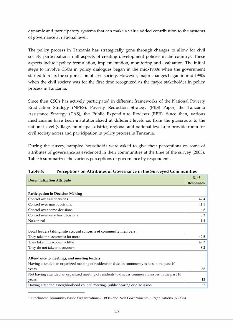
During the survey, sampled households were asked to give their perceptions on some of
attributes of governance as evidenced in their communities at the time of the survey (2005).
Table 6 summarizes the various perceptions of governance by respondents.
Table 6: Perceptions on Attributes of Governance in the Surveyed Communities
Decentralization Attribute % of
Responses
Participation in Decision Making
Control over all decisions 47.4
Control over most decisions 41.1
Control over some decisions 6.8
Control over very few decisions 3.3
No control 1.4
Local leaders taking into account concerns of community members
They take into account a lot more 42.5
They take into account a little 49.3
They do not take into account 8.2
Attendance to meetings, and meeting leaders
Having attended an organized meeting of residents to discuss community issues in the past 10
years
88
Not having attended an organized meeting of residents to discuss community issues in the past 10
years
12
Having attended a neighborhood council meeting, public hearing or discussion 62
5 It includes Community Based Organizations (CBOs) and Non Governmental Organizations (NGOs)

26
Decentralization Attribute % of
Responses
Not having attended a neighborhood council meeting, public hearing or discussion 38
Having met a local politician, called him/her, or sent a letter 48
Not having met a local politician, called him/her, or sent a letter 52
Having met a national politician, called him/her, or sent a letter 23
Not having met a national politician, called him/her, or sent a letter 77
Having signed a petition to make a demand from local or national government 6
Not having signed a petition to make a demand from local or national government 94
Participated in a protest or demonstration 9
Not having participated in a protest or demonstration 91
Participated in an information or election campaign 39
Not having participated in an information or election campaign 61
Interests of National and Local Leaders
The county (Tanzania) is run for all the people 75
The country (Tanzania) is run by a few for their own interests 25
The local government is run for all the people 76
The local government is run by a few for their own interests 24
Democracy and Elections
Voted in the last state/national/presidential elections 91
Did not vote in the last state/national/presidential elections 9
Perceived the elections to be fair and free 89
Did not perceive the elections to be fair and free 11
Very satisfied with the way democracy woks in this country 55
Somewhat satisfied with the way democracy woks in this country 40
Somewhat dissatisfied with the way democracy woks in this country 4
Very dissatisfied with the way democracy woks in this country 1
Corruption
Almost no government official is involved in bribe taking and corruption 16
A few government officials are involved in bribe taking and corruption 57
Most government officials are involved in bribe taking and corruption 19
Almost all government official are involved in bribe taking and corruption 8
Confidence with officials/leaders
Confidence with local government officials 80
No confidence with local government officials 20
Confidence with national government officials 92
No confidence with national government officials 8
Confidence with doctors and nurses in health clinics 88
No confidence with doctors and nurses in health clinics 12
Confidence with teachers and school officials 91
No confidence with teachers and school officials 9
Confidence with the police 62
No confidence with the police 38
Confidence with Judges and staff of the court 62
No confidence with Judges and staff of the court 38
Confidence with staff of NGOs 90
No confidence with staff of NGOs 10

27
Judging from the perceptions of the sampled individuals in the surveyed communities, it
was evident that there has been substantial improvement in the level of participation of the
people at the grassroots in decision-making. Many of the individuals interviewed believed
that they had control in most of the decisions reached in the communities. It was also highly
perceived that local leaders take into account the concerns of community members. The level
of participation in meetings, and contacts between community members and their leaders
was high. Community members had confidence in their leaders both at national and local
government levels. Participation in elections, which were perceived by the majority to be
free and fair, was also high, and generally, community members were satisfied with the way
democracy was working. As for corruption, it was perceived by more than half of the
sampled individuals that only a few government officials are involved in bribe taking and
corruption.
Despite the above achievements in terms of participation in decision-making and high level
of commitment on the part of local leaders, the governance weakness in the study areas
centers was more evident on lack of facilities and the neglect of the local leadership by the
centre. It was also evident that the working methods in the administration and management
of public functions are normally unreliable and have not been adjusted to global changes.
Local leaders do not have the necessary support to enable them undertake their duties
effectively. Apart from the Village Executive Officers (VEOs), the rest do not get paid wages
and they therefore end up misusing rent from their fellow villagers or charging for their
services. As a result, such incidences push people back into poverty.
Lack of access to external information (including market information) is a critical constraint
in the rural. Community members rely mostly on their leaders, relatives, friends and
neighbors for update information. During the survey, when asked how many times any
member of the sampled households had read a newspaper in the past one month, 70 percent
responded that no one had. Only about 10 percent had read a newspaper once in the entire
month. As a result of poor access to information, in some cases there is a big time lag
between the time when decisions are taken at the centre and when the information reaches
the implementers or the people at the grassroots. Thus, it seems as though, despite efforts to
transfer powers to the grassroots, there has been no transfer of capabilities required to
control local resources and use them to transform rural communities, and therefore, good
governance that seems to prevail in the study area has yet to contribute substantially
towards mobility out of poverty.
5.2 Public Socio-Economic Services and Mobility
First, in-access to public services (including education; health; water; infrastructure particularly
roads, markets and market information about demand for crop products, supply/availability
of inputs, and prices; financial services such as banking facilities, or credit facilities
(including input credit) and informal financial services; security; and information

28
particularly awareness about various community wide issues), availability of the services to
the community members and gender dimensions in services were mentioned as critical
bottlenecks of mobility out of poverty.
Second, reliability and adequacy of the services; largely focusing on the quality of services and
effectiveness in service delivery; third; source/origin of services; essentially, who provides
which services? Is it the government, private operators, or other non-state actors?; and
fourth; involvement of communities and their participation in public services delivery;
with particular emphasis on the aspect of community participation as an essential element of
sustainability.
5.2.1 Un-met Needs to Access to Services
With regard to health, there have also been major improvements over the past decade, but
there are some gaps still to be worked out. For example some communities had health
facility (dispensary) within their villages, while others had no health facilities within their
localities. Traditional healers still play an important role in the communities, and traditional
birth attendants are still popular in these communities as well.
The major gap identified with regard to health services in the studied communities is the
issue of proximity, and affordability, which entails, not only the medication costs, but also
the other related costs – particularly transport, especially where the patient has to be taken
to a hospital – and not a dispensary or a health centre. About 33.2 percent of the interviewed
households indicated that it was difficult for them to get the medical services because the
services are too expensive. On the other hand, 28.9 percent of the respondents indicated that
it was difficult to get health services because the medical facilities are too far. Only 2.7
percent of the respondents pointed to poor quality of the medical facilities in this regard.
Transport cost was noted as a significant barrier to accessing health services in all
communities, especially in the focus group discussions. The respondents indicated that,
even in the cases where the household was not supposed to bear much of the treatment costs
– as for the case of TB for instance, transport costs and other related costs were very
significant, and were hampering access to health services.
The major problem in all the studied communities was access to clean water. The problem of
water in these communities had explicit gender dimension to it, since the burden was
largely born by women and children. Shortage of water affects other important economic
activities in the communities, especially agriculture, by using many hours of the important
labor force in the households. Besides, lack of enough water in some communities was also
among the factors contributing to the problems of diseases, particularly trachoma. Water
shortage in the communities has been a contributing factor to the growing problem of
trachoma in some parts of central Tanzania (FGD, Muhalala Village).

29
The problem of water was also linked to domestic violence in some communities. This is
particularly the case because of the gender dimensions involved in it. Women and children
are the ones responsible for collection of water, usually from long distances, and could take
several hours. And when it becomes too long, men become suspicious that their wives are
not just fetching water, but up to something else. The following experiences from Makale
Village indicate the severity of the water problem, its gender dimension and associated
domestic conflict (Zenaida, 45 years, Women FGD – Makale Village, August, 2005).
Access to infrastructure and other important economic services was a serious problem in the
studied communities. Due to poor roads, and limited capacity of the private sector service
providers in the respective villages, public transport remains one of the major constraints in
the studied communities (Perhaps, the private investors are also discouraged by low
effective demand by the villagers due to low incomes in these villages).
Another important aspect with regard to information is awareness about HIV/AIDS issues.
Still, in those communities, AIDS related deaths are linked to witchcraft beliefs. The
following quote from Makale community exemplifies the situation ‚<<.Many people are
not well informed about HIV/AIDS in this community. There is this belief that people dying
of AIDS in this village are bewitched. Someone could die of AIDS today, and in few days,
his or her spouse, who has been left behind, would be dated by some other person in the
village‛ (FGD, Makale Village):
5.2.2 Adequacy and Reliability of Services
The major challenge that exists is the inadequacy of basic social service provision i.e quality
of basic education. While there are efforts to build classrooms and desks through the
Primary Education Development Plan (PEDP), there are still no enough teachers in the
schools. For instance, during the study period, Kidarafa village had three primary schools,
but one of the schools had only one teacher. With regard to health, it is appreciated by the
communities that the government has constructed dispensaries and introduced mobile
clinics to meet growing need for maternal and child health in the villages. About 53.7
percent of the interviewed households indicated that the health situation in their
communities had improved whereas 32 percent of the respondents indicated that there has
been no change in health situation over the past decade in their communities. Further, 13.9
percent thought that the situation had deteriorated. However, at individual level, only 30
percent of the respondents indicated that their health conditions had improved over the past
ten years. It is obvious that one major challenge in addressing the quality of health services.
5.2.3 Key Players of Service Providers
One aspect that was noted in the study is the limited number of players in the rural settings.
Generally, most services are provided by the government, with very limited
supplementation from other players particularly the private sector. For each of the studied
villages, the nearest secondary school was actually a public school, signaling limited

30
participation of private providers in secondary education in the rural areas. With regard to
health services, the nearest reliable health facilities to the communities were either owned by
the government or religious organizations. Religious organizations have been playing
important role in reducing the gap in health services between what the government delivers
to the community members and the actual needs of the communities. So the same for water
services, TCRS installed a windmill in Kidarafa community, the only reliable source of water
in the village.
5.2.4 Community Participation in Services
Community participation is an important attribute for sustainability of social services
projects – particularly water and education. One remarkable achievement of the Primary
Education Development Plan (PEDP) was the involvement of the communities, and
subsequent community participation in the actual implementation on the ground. In all the
studied communities, the villagers considered themselves as the ‘effective owners’ of the
schools, since they participated in the re-structuring, and had much say in the day to day
running of the schools.
Table 7: Definition of Community and Household Variables
Dependent Variables Definition of the Variables
Status A continuous variable measuring the poverty status/welfare of the household in
relation to the step on the ladder which the household was at the time of survey
Non-poor = 1 if the status of household is above the cutoff point (poverty line) defined by
respondents in a focus group discussions in every community; else = 0
Independent Variables
Household Characteristics
Age Age of the head of the household
Agesq The square of the age of the head of the household
Sex = 1 if male; else = 0
Hhsize Household size
NoschIL = 1 if has no school and illiterate; else = 0
NoschLI = 1 if has no school but literate; else = 0
Primcomp = 1 if has completed primary school; else = 0
Secincomp = 1 if has incomplete secondary education; else = 0
Seccopm = 1 if has completed secondary education; else = 0
Univ = 1 if has university education; else = 0
Trader = 1 if the respondent was a trader; else = 0
Land Land owned (acres)
Oxen =1 if owns oxen; else = 0
Cow =1 if owns cow; else = 0
Mule =1 if owns mule; else = 0
Goat =1 if owns goat; else = 0
Pig =1 if owns pig; else = 0
Chicken =1 if owns chicken; else = 0
Animcar =1 if owns animal driven car; = 0
Bicy =1 if owns bicycle; else = 0
Radio =1 if owns radio; else = 0
Kerosene =1 if owns kerosene cooker; else = 0

31
Dependent Variables Definition of the Variables
Sewing =1 if owns sewing machine; else = 0
Tapin =1 if have tap water connection in the house; else = 0
Privwell =1 if have a private well; else = 0
Rooms Number of rooms in the main house
Latrine =1 if own a latrine; else = 0
Wall =1 if wall made of brick or concrete; else = 0
Roof =1 if roof made of concrete or irons sheets; else = 0
Econassoc =1 if member of any economic association; else = 0
Creditassoc =1 if member of any credit association; else = 0
Politassoc =1 if member of any political association; else = 0
Religassoc =1 if member of any Religious association; else = 0
Creditcons =1 if received credit for consumption; else = 0
StatusNP Step on the ladder of life in relation to power
StatusNH Step on the ladder of life in relation to happiness
Asset Aggregate measure of asset
Ammen Aggregate measure of amenities
Livest Aggregate measure of livestock measured in livestock units
Household Shocks
Health = 1 if experienced a health shock; else = 0
Community Characteristics
Dailymak = 1 if there is daily market in the community; else = 0
Transmark = 1 if there is transport through the daily market; else = 0
Distmark Distance to the daily market (km)
Periodmark = 1 if there is periodic market in the community; else = 0
Disp = 1 if there is dispensary in the community; else = 0
HealthC = 1 if there is health centre in the community; else = 0
Disthosp Distance to the nearby hospital (km)
Healthworker = 1 if there is a health worker based in the community; else = 0

32
6.0 CONCLUSIONS AND POLICY IMPLICATIONS
One can therefore see clearly that poverty shocks are real factors affecting mobility of
members of the communities in Tanzania. While a few shocks are desirable in that they
promote community prosperity, many of them are obstacles to community economic and
social development. They impose serious intricacies to development and welfare of the
people. This is particularly so because most of the people in the study area were vulnerable
to shocks given their limited risk management potentials. Climatic change, economic
hardships, and health related problems are among the key mentioned shocks prohibiting out
of poverty escape routes.
The major identified gaps with regard to poverty escape routes include inadequate health
services, lack of access to clean water, quality of basic education, and limited number of
players in the rural settings. It is important that pro-poor policies are implemented to
alleviate health service, clean water, quality of education, and transport problems. The fact
that the government alone can’t afford overcoming the shortcomings, other development
stakeholders should consider refocusing resources in rural areas.
As part of the emerging issues, good governance was mentioned a prerequisite for sound
rural development management. The devolution of power to sub-national governments has
been popularized and promoted by development partners. Promoting good governance at
all levels in the policy implementation will accelerate poverty upward mobility in the
region.

33
REFERENCES
Economic and Social Research Foundation (ESRF) (2006). ‚Private Sector Development Strategy for
Tanzania: Diagnostic Analysis and Outline of the Proposed Development Strategy‛ Draft, ESRF, Dar-
es-Salaam
Hughes, D and K. DuMont. 1993. ‚Using Focus Groups to Facilitate Culturally Anchored Research.‛
American Journal of Community Psychology 21(6):775-806.
Jahnke. H. E. (1982). Livestock Production Systems and Livestock Development in Tropical Africa. Kieler
Wissenschaftsverlag Vauk.
Krueger, A. R. 1994. Focus Groups: A Practical Guide for Applied Research. SAGE Publications. London.
Laderchi, C. R., R. Saith and F. Stewart. (2003). ‚Does it Matter that We Do Not Agree on the Definition of
Poverty? A Comparison of Four Approaches.‛ Oxford Development Studies, 31 (3): 243-274.
Msambichaka, L. A., N. E. Mwamba and O. J. Mashindano (2005). Poverty in Tanzania: Situation,
Perception and Escape Routes, Tanzania Journal of Population Studies, Vol. No. Dar-es-Salaam
Rao, V. (1998). ‚Wife-Abuse, its Causes and its Impact on Intra-Household Resource Allocation in Rural
Karnataka: A ‘Participatory Econometric Analysis’.‛ In Gender, Population and Development. Delhi: Oxford
University Press.
Temu, A.E and J. M. Due.2000. ‚Participatory Appraisal Approaches versus Sample Survey Data
Collection: A Case of Smallholder Farmers Well-being Ranking in Njombe District, Tanzania.‛ Journal
of African Economies 19(1): 44-62.
URT . 1998. ‚Participatory Poverty Assessment—Shinyanga Region.‛ Dar es Salaam: UNDP.
URT . 1999. ‚Poverty and Welfare Monitoring Indicators.‛ Dar es Salaam: Vice Presidents Office.
URT . 2000. ‚Poverty Reduction Strategy Paper.‛ Dar es Salaam: Vice President’s Office.
URT . 2002. ‚Household Budget Survey – 2000/2001.‛ Dar es Salaam: National Bureau of Statistics and
Presidents Office-Planning and Privatization.
URT . 2004a. National AIDS Control Program: HIV/AIDS/STI Surveillance Report – Report No 18. Dar es
Salaam: Ministry of Health.
URT . 2004b. ‚Vulnerability and Resilience to Poverty in Tanzania: Causes, Consequences and Policy
Implications.‛ TzPPA Main Report. Dar es Salaam: Vice President’s Office.
URT . 2004c. ‚Agricultural Marketing in Tanzania: Sector Position Paper‛, Ministry of Cooperatives and
Marketing, Dodoma
URT . 2005. ‚Poverty and Human Development Report-2005.) Dar es Salaam: Research and Analysis
Working Group.

34
ESRF PUBLICATIONS
Discussion Papers
1. The Role of Mobile Phones on Sustainable Livelihood. A.K. Hassan and Dora
Semkwiji, August 2011
2. Inter Household Private Income Transfers and Poverty in Tanzania. Nassoro Hussein
and John Kajiba. September 2011
3. Improving Public Private Partnership (PPP) in Health Services Delivery in Tanzania:
Successes and Constraints. Dr. O.Mashindano, Dr. F Kessy and Prof. Josephat Itika,
September 2011
4. Poverty Escape Routes in Central Tanzania: Coping Strategies in Singida and
Dodoma Regions (Volume 1). Dr. O. Mashindano; Dr. F. Kessy; Prosper Charles and
Dennis Rweyemamu, September 2011.
5. Poverty Escape Routes in Central Tanzania: Coping Strategies in Singida and
Dodoma Regions (Volume 2). Dr. O. Mashindano; Dr. F. Kessy; Prosper Charles and
Dennis Rweyemamu, September 2011.
6. Poverty Escape Routes in Central Tanzania: Coping Strategies in Singida and
Dodoma Regions (Volume 3). Dr. O. Mashindano; Dr. F. Kessy; Prosper Charles and
Dennis Rweyemamu, September 2011.
7. Aligning and Harmonizing the Livestock and Land Policies in Tanzania. Dr. Furaha
Lugoe, September 2011
8. The Impact of Globalization on the Labour Market: A Case Study of Tanzania.
Working Paper Series No. 18. Beatrice Kalinda Mkenda. September 2006.
9. Capital Markets: The Case of Tanzania. Working Paper Series No. 19. Allan Syril
Mlulla. October 2006.
10. Globalization and Rural Household Welfare in Tanzania. Working Paper Series No.
15. Beatrice Kalinda Mkenda. August 2005.
11. Agricultural Marketing and Supply Chain Management in Tanzania: A Case Study.
Working Paper Series No. 16. Elina Eskola 2005.
12. Analysis of Factors Hindering FDI Flow into the Agricultural Sector in Tanzania.
Working Paper Series No. 17. David A. Nyange. 2005.

35
Policy Dialogue Series
1 Strengthening Microenterprises in Tanzania: The Case of Small Scale Vegetables in
Arusha Dr. O. Mashindano; Dr. B. Mkenda and Vivian Kazi, September 2011
2 Experience of Tanzania and Uganda in the use of Research based Evidence to
Influence Policy Vivian Kazi, September 2011
3 Trade, Development and Poverty: The Case of the Textile Industry, by Dr. Josaphat
Kweka and George Kabelwa (2006).
4 Trade, Development and Poverty: The Case of the Fishery Industry, by Dr.
Josaphat Kweka and George Kabelwa (2006).
5 Measuring the Impact of HIV/AIDS on the Electoral Process in Tanzania, by Flora
Kessy, Ernest Mallya and Dr. Oswald Mashindano (2006).
Quarterly Economic Reviews (QER)
1. QER Volume 10 Issue 3 for July – Sept, 2010
2. QER Volume 10 Issue 2 for Apr – Jun, 2010
3. QER Volume 10 Issue 1 for Jan – Mar, 2010
4. QER Volume 9 Issue 4 for Oct Dec, 2009
Annual Reports
1. ESRF Annual Report, 2010
2. ESRF Annual Report, 2009
3. ESRF Annual Report, 2008
4. ESRF Annual Report, 2007
5. ESRF Annual Report, 2006
6. ESRF Annual Report, 2005
Newsletters
1. Newsletter Volume 10 – Issue 1, 2011
2. Newsletter Volume 9 – Issue 2, 2010
3. Newsletter Volume 9 – Issue 1, 2010
4. Newsletter Volume 8 – Issue 2, 2009
5. Newsletter Volume 8 – Issue 1, 2009

36
Policy Brief Series
1 The Land Factor in Mining Gold Reserves in Tanzania. Dr Furaha Lugoe, September
2011
2 Governance Breakdown in the Urban Malaria Control: Policy Reflections in the
Outburst of Msimbazi Valley Mosquito, Dar es Salaam. Dr. Francis Mwaijande,
September 2011
3 Value Chain Analysis of Grapes Sub-sector. Vivian Kazi and Dr. O. Mashindano,
September 2011
TAKNET Policy Brief Series
1. Growth and Poverty Reduction in Tanzania: Why such a mismatch? Moderated by
Dr. Oswald Mashindano – 2009.
2. The Impact of Information and Communication Technology (ICT) on Rural
Livelihoods. Moderated by Abdallah K. Hassan – 2009.
3. Foreign Direct Investment Incentive Package in Tanzania. Moderated by Festo Maro
– 2009
4. Tatizo la Walemavu wa Ngozi (Albino) Tanzania: Nini Kifanyike? Synthesized by
Dora Semkwiji, 2009
5. Petroleum Policy and Constitutional Paradox in the United Republic of Tanzania.
Moderated by Festo Maro, 2009
6. Social Welfare and Aging in Tanzania: Moderated by Festo Maro and Synthesized
by Deogratias Mutalemwa
7. Tanzanian Cultural Environment and Economic Development: Moderated by Festo
Maro and Views summarized by Deogratias Mutalemwa
8. School Competition and Student Learning Rights: Moderated by Dr. Donatilla
Kaino and views synthesized by Joseph Ibreck
9. Informal Sector Taxation in Tanzania: Moderated by Apronius Mbilinyi;
Synthesized by: Deogratias Mutalemwa

37
10. Msongamano wa Magari Jijini Dar es Salaam, Nini kifanyike? Moderated and
sythesized by Boniface Makene
11. Importation of Counterfeit Products: What should be done? Moderated by
Deogratias Kishombo, Synthesized by: Deogratias Mutalemwa
12. Vifo vya Akina mama kutokana na matatizo ya ujauzito (maternal mortality) ni
tatizo kubwa Tanzania: nini kifanyike kutatua tatizo hili? Moderated by Dr. Tausi
Kida and Dr. Riziki Ponsiano
13. Tanzania National Poverty Reduction Framework – MKUKUTA what are the
lessons: Moderated by Dr. O. Mashindano and views synthesized by Apronius
Mbilinyi
14. The Effect of the Global Financial crisis and the Way Forward for Tanzania.
Moderated by Dr. Donatila Kaino, 2009
15. What will be the Impact of the 2009/2010 Government Budget to Economic Growth
and Poverty Reduction? Moderated by Dr. H. Bohela Lunogelo, 2009
16. Social Protection and Ageing in Tanzania. Moderated by Festo Maro, 2009
17. What Benefits can Tanzania Derive from the East African Common Market (EACM)
arrangement: Moderated by Festo Maro and Monica Hangi

38
APPENDIX I: DETAILS OF REGRESSION RESULTS FOR VOL. I & II
Table A- 1: Frequencies of the Variables used in Regression Analysis
Variables Percent (N=309)
Male head of the household 86.8
Non poor households 36.4
No school and illiterate 15.9
No school but literate 2.8
Completed primary school 56.6
Completed secondary education 2.5
University education 2.5
Trader as a primary occupation 10.7
Animal car 8.2
Bicycle 59.1
Radio 64.2
Milling machine 3.3
Kerosene 5.5
Sewing 4.6
Private well 1.2
Latrine 85.1
Flush toilet 4.6
Type of wall 29.5
Type of roof 46.5
Member to economic associations 14.9
Member to credit associations 5.2
Member to political associations 30.4
Member to Religious associations 18.1
Aggregate measure of asset 77.1
Aggregate measure of amenities 94.9
Aggregate measure of membership to associations 41.1
Health shock 51.4
Received credit for consumption 24.5
Daily market in the community 37.1
Daily transport past the market 89.3
Period market in the community 45.6
Dispensary located in the community 47.8
Health Centre located in the community 33.7
Health worker based in the community 50.0
Table A- 2: Descriptive Statistics of the Variables used in the Analysis
Variables N = 309
Mean Minimum Maximum
Step on the ladder of life in relation to welfare 4.0 (2.1) 1 10
Step on the ladder of life in relation to power 4.9 (2.6) 1 10
Step on the ladder of life in relation to happiness 5.2 (2.5) 1 10
Age of the head of household 44.4 (13.6) 12 97
Household size 5.7 (2.7) 1 21
Land owned (acres) 9.3 (14.8) 0 127

39
Variables N = 309
Mean Minimum Maximum
Oxen 0.3 (1.0) 0 8
Cow 2.2 (6.5) 0 60
Mules 0.1 (0.7) 0 7
Goats 2.6 (4.9) 0 32
Sheep 0.6 (2.3) 0 27
Pigs 0.3 (1.7) 0 15
Chicken 6.3 (8.9) 0 84
Number of rooms in the main house 3.0 (1.8) 0 16
Aggregate measure of livestock/Livestock units 2.4 (5.4) 0 45
Distance to the daily market (km) 10.0 (11.6) 0 36
Distance to the nearby hospital (km) 22.8 (15.9) 5 50
(a) Standard deviations are in parenthesis.
Table A- 3: Regression Analysis Results (Model 1)
Variables Coefficient Standard Error t-statistic
Household size -0.025 0.044 -0.57
Sex 0.192 0.286 0.67
Age -0.044 0.041 -1.07
Agesqr 0.000 0.000 1.25
NoschIL 0.166 0.382 0.44
NoschLI 1.385* 0.786 1.76
Primcomp 0.589** 0.293 2.00
Secincomp 0.618 0.746 0.83
Seccomp 1.431** 0.653 2.19
Univ 1.887*** 0.565 3.33
Yearedu 0.026 0.057 0.46
Trader -0.014 0.280 -0.05
Animcar 0.033 0.335 0.10
Bicy -0.339 0.243 -1.40
Radio 0.408 0.271 1.50
Kerosi 0.388 0.413 0.94
Sewing -0.008 0.513 -0.02
Milling 1.253** 0.557 2.25
Oxen 0.046 0.104 0.44
Cow 0.011 0.032 0.35
Mule -0.088 0.160 -0.56
Goat 0.066*** 0.022 2.91
Sheep 0.071* 0.040 1.76
Pig -0.019 0.057 -0.34
Chick -0.010 0.133 -0.81
Land -0.000 0.007 -0.12
Tapin 2.449** 1.161 2.11
Privwell 0.118 1.319 0.09
Rooms -0.033 0.063 -0.53
Flutoil 0.114 0.474 0.24
Latrine 0.134 0.310 0.43

40
Variables Coefficient Standard Error t-statistic
Wall 0.633*** 0.221 2.86
Roof 0.584*** 0.208 2.80
Creditcons -0.126 0.197 -0.64
Health 0.001 0.002 0.54
Econassoc -0.236 0.454 -0.52
Creditassoc -0.230 0.492 -0.47
Politassoc 0.490 0.340 1.44
Religassoc 0.386 0.289 1.33
StatusNP 0.195*** 0.043 4.47
StatusNH 0.195*** 0.041 4.70
Distmark -0.035 0.016 -2.12
Periodmark 0.385 0.321 1.20
Transmark 0.468 0.677 0.69
Disp -0.954 0.701 -1.36
HeaC 1.564*** 0.501 3.12
Disthosp -0.003 0.003 -1.07
Heaworker -0.513 0.362 -1.42
Asset -0.028 0.355 -0.08
Ammen -0.325 0.494 -0.66
Assoc 0.473 0.396 1.20
Livest 0.027 0.041 0.67
R-squared = 0.65, Adjusted R-squared = 0.56, observations=309.
* shows significance at 10% level
** shows significance at 5% level
*** shows significance at 1% level

41
Table A- 4: Regression Analysis Results (Model 2)
Variables Coefficient Standard Error t-statistic
Household size 0.005 0.039 0.14
Sex 0.245 0.290 0.85
Age -0.058 0.041 -1.41
Agesq 0.000 0.000 1.54
Yearsedu 0.079** 0.038 2.05
Trader 0.130 0.276 0.47
Creditcons -0.195 0.197 -0.99
Health 0.000 0.002 0.38
StatusNP 0.193*** 0.042 4.53
StatusNH 0.255*** 0.041 6.15
Distmark -0.028* 0.162 -1.73
Periodmark 0.372 0.316 1.18
Transmark 0.447 0.663 0.67
Disp -0.633 0.585 -1.08
HeaC 1.367*** 0.334 4.09
Disthosp -0.001 0.003 -0.39
Heaworker -0.393 0.332 -1.18
Asset 0.337 0.225 1.50
Ammen 0.228 0.382 0.60
Assoc 0.084 0.231 0.37
Livest 0.068*** 0.016 4.06
R-squared = 0.55, Adjusted R-squared = 0.52, observations=309;
* shows significance at 10% level
** shows significance at 5% level
*** shows significance at 1% level
Table A- 5: Regression Analysis Results (Model 3)
Variables Odds Ratio Robust Standard Error Z
Household size 0.845 0.102 -1.38
Sex 0.338 0.242 -1.51
Age 0.907 0.075 -1.17
Agesq 1.001 0.001 1.38
NoschIL 0.768 0.736 -0.28
NoschLI 30.522** 40.423 2.58
Primcomp 1.768 1.185 0.85
Secincomp 8.373* 11.082 1.61
Seccomp 22.601** 26.906 2.62
Univ 57.677*** 56.921 4.11
Yearsedu 1.035 0.111 0.32
Trader 0.548 0.352 -0.93
Animcar 0.843 0.912 -0.16
Bicy 0.119*** 0.070 -3.61
Radio 1.673 1.242 0.69
Kerosi 1.079 0.817 0.10
Sewing 0.367 0.3555 -1.03
Milling 4.240 3.899 1.57
Oxen 0.884 0.223 -0.49
Cow 0.951 0.075 -0.64

42
Variables Odds Ratio Robust Standard Error Z
Mule 0.413* 0.202 -1.80
Goat 1.335*** 0.116 3.34
Sheep 0.898 0.160 -0.60
Pig 1.076 0.173 0.46
Chick 0.967 0.034 -0.95
Land 1.026 0.021 1.23
Privwell 9.993 25.585 0.90
Rooms 0.967 0.174 -0.18
Flutoil 0.587 0.531 -.059
Latrine 0.487 0.489 -0.72
Wall 1.998 1.067 1.30
Roof 3.313** 1.586 2.50
Creditoons 0.981 0.459 -0.04
Health 1.007 0.005 1.32
Econassoc 0.937 1.118 -0.05
Creditassoc 4.716 7.969 0.92
Politassoc 1.290 0.912 0.36
Religassoc 1.473 0.986 0.58
StatusNP 1.278** 0.130 2.41
StatusNH 1.705*** 0.207 4.39
Distmark 0.871** 0.050 -2.38
Periodmark 35.248** 44.994 2.79
Transmark 53.763 141.416 1.51
Disp 7.673 17.767 0.88
HeaC 0.898 1.272 -0.08
Disthosp 1.009 0.011 0.94
Heaworker 0.333 0.303 -1.21
Asset 1.906 1.754 0.70
Ammen 2.286 3.477 0.54
Assoc 0.623 0.639 -0.46
Livest 1.074 0.085 0.90
Pseudo R-squared = 0.51, observations=307, Log pseudo-likelihood = -97.4485;
* shows significance at 10% level
** shows significance at 5% level
*** shows significance at 1% level
Table A- 6: Regression Analysis Results (Model 4)
Variables Odds Ratio Robust Standard Error Z
Household size 0.927 0.058 -1.21
Sex 0.452 0.257 -1.40
Age 0.938 0.062 -0.96
Agesq 1.001 0.001 1.10
Yearsedu 1.108 0.080 1.41
Trader 0.609 0.296 -1.2
Creditcons 0.938 0.343 -0.17
Health 1.004 0.004 1.01
StatusNP 1.197** 0.093 2.32
StatusNH 1.621*** 0.134 5.85

43
Variables Odds Ratio Robust Standard Error Z
Distmark 0.911** 0.033 -2.56
Periodmark 9.969*** 7.304 3.14
Transmark 7.069 11.460 1.21
Disp 2.763 3.256 0.86
HeaC 0.983 0.619 -0.03
Disthosp 1.011 0.007 1.59
Heaworker 1.049 0.736 0.07
Asset 1.537 0.773 0.85
Ammend 1.386 0.909 0.50
Assoc 1.129 0.494 0.28
Livest 1.068** 0.032 2.18
Land 1.105 0.017 0.93
Pseudo R-squared = 0.35, observations=309, Log pseudo-likelihood = -131.2101;
* shows significance at 10% level
** shows significance at 5% level
*** shows significance at 1% level

44