Potential economic effects of TTIP for the Netherlandsand the EU

Hugo Rojas-Romagosa

CPB Discussion Paper | 331

Potential economic effects of TTIP for the Netherlandsand the EU

Hugo Rojas-Romagosa*

CPB Netherlands Bureau for Economic Policy Analysis

June 2016

Abstract

The Transatlantic Trade and Investment Partnership (TTIP) is a comprehen-sive preferential trade agreement that is expected to have a significant effect inEU and US bilateral trade and investment relations. Negotiations are ongoing,so we use a scenario analysis to estimate the potential effects of TTIP underlikely negotiated outcomes. In our main scenario, we assume a final trade dealwhere current tariffs are eliminated and non-tariff barriers are significantly re-duced. Using a CGE model (WorldScan) we simulate the potential economiceffects for the Netherlands. We find that US-Dutch bilateral trade doubles andthis is translated into a positive but moderate effect on income of 1.7% for theNetherlands by the year 2030. These potential gains are higher than those forthe EU and the US (both around 1%).

Keywords: TTIP, preferential trade agreements, CGE modelsJEL Classification: F13, F17, C68

1 IntroductionThe Transatlantic Trade and Investment Partnership (TTIP) is currently being ne-gotiated between the European Union (EU) and the United States (US). This deepintegration agreement consists of three main pillars: eliminating tariffs, regulatorycooperation to reduce non-tariff barriers (NTBs)1, and other behind the borderrules. Of these, the first two components will have direct economic impacts, and itis expected that the NTB reductions related to TTIP will yield the most economicimpact (Francois et al., 2013; Egger et al., 2015).

*I would like to thank Joseph Francois and Miriam Manchin for providing me with the STATAcode for the NTB estimations; Albert van der Horst, Clemens Kool and Gerdien Meijerink forvaluable comments, and Emelie Walraven for research assistance.

1NTBs are also referred to as non-tariff measures (NTMs) and/or technical barriers to trade(TBTs).

1

Since the EU and the US economies account for roughly half of world outputand world trade, the scope and international impact of TTIP is considerable. Therelatively large integration of both blocs has been the result of the post-war tradeliberalisation process, which also included a significant increase in transatlantic in-vestments – both blocs are also each other’s most important investment partners.2This trade liberalisation process, however, has been mostly driven by the reductionof tariff rates. With relatively low tariffs levels at present, the economic focus ofTTIP has shifted to the reduction of the biggest remaining hurdles in transatlantictrade: non-tariff barriers (NTBs). Thus, a comprehensive agreement that includesNTBs is expected to provide the most economic impact.

Much of the general debate on TTIP, however, has focused on the desirability ofregulatory convergence and other political topics. Although these issues are centralto the negotiations on TTIP, and the political aftermath of the negotiations, in thispaper we focus our analysis exclusively on the economic perspective.3

The main objective of this paper, therefore, is to analyse the potential eco-nomic effects of TTIP for the Netherlands. To achieve this goal we start by a shortdescription of the main economic elements being negotiated under TTIP and theirpotential economic effects. We then summarise the main studies that have estimatedthe economic effects of TTIP. However, these previous TTIP studies have focusedon the overall gains for the EU and some of the larger EU countries.4 Therefore, inthis study we use WorldScan –the CPB in-house computational general equilibrium(CGE) model– to assess the potential economic effects of TTIP for the Netherlands.As part of the TTIP simulations, we have two main policy shocks: elimination oftariffs between the US and all EU countries and reduction in NTB costs. For thesecond shock, we follow the recent methodological approach in Egger et al. (2015)to estimate the expected NTB reductions associated from TTIP. In our "full" TTIPsimulation we combine the previous two policy shocks to have both the tariff elimi-nation and the NTB cost reductions.

We find macroeconomic effects for the US and for the aggregated EU regionthat are similar to previous CGE studies (Francois et al., 2013; Egger et al., 2015).For the Netherlands, we find that GDP and consumption per capita increase bythe year 2030 by more than the EU average, by 1.7% and 3.1% respectively. ThisGDP increase is driven by a strong surge of bilateral trade between the US and theEU, which is expected to double: EU exports to the US increase by 111%, while USexports to the EU raise by 119%. Dutch exports to the US increase by 95%, but totalexports (to all destinations) increase by a more moderate 4%. TTIP also creates,therefore, strong trade diversion patterns and Dutch exports to other EU countries

2When each individual EU country is analysed separately, however, intra-EU trade representsthe majority of EU countries’ trade flows. For the Netherlands, intra-EU trade represents around70% of total trade and US trade is around 7%.

3See Ecorys (2016) for the potential environmental and social effects of TTIP.4Studies that analysed the specific results for The Netherlands are Ecorys (2012, 2016). These

studies are based on the same CGE modelling as in Francois et al. (2013) and another methodologyto estimate NTB reductions associated with TTIP, which yields NTB information for a limitednumber of sectors (cf. Berden and Francois, 2015).

2

decreases by 2% and to third regions by roughly 3%. These trade diversion effectsalso result in a relatively small decrease in trade and GDP for non-TTIP regions.

With respect to the labour market, our simulations show that with a full TTIPscenario that eliminates tariffs and reduces NTBs, Dutch average wages will increaseby more than 2%. More importantly, the wages of both low- and high-skill workersare expected to rise. This implies that TTIP will not significantly affect wage norincome inequality. The sectoral reorganisation of production, however, implies thatworkers in declining sectors will need to relocate to other sectors. This labourdisplacement will have short term adjustment costs for those workers that need tochange employment. However, these additional costs are relatively small, since onlya small proportion of workers would have to change jobs and move from one sectorto another, in comparison to the job creation and destruction that occurs on a yearlybasis. In particular, we expect that about 1.5% of total jobs (around 114,000 jobs)will be reallocated to other sectors in a 13 year period, while on a yearly basis,13% of total jobs (around one million jobs) are either created or destroyed in theNetherlands (Brull et al., 2010).5

Finally, it is important to mention that these potential effects are likely to under-estimate the full economic effects of TTIP, since our methodology does not analyseadditional economic effects of TTIP related to public procurement provisions, in-creased FDI and dynamic effects from trade.

This paper proceeds as follows. We first explain in Section 2 the main character-istics of TTIP and we list the potential economic effects. In Section 3 we summarisethe main results of the economic studies that have analysed TTIP. We then explainin Section 4 the WorldScan CGE model, how the TTIP experiment is modelled andwhat are the main economic results for the Netherlands. In Section 5 we discusssome additional economic effects related to TTIP and we conclude in Section 6.

2 TTIP and its potential economic outcomes

2.1 What is TTIP?

The setup of TTIP is to become a deep and comprehensive preferential trade agree-ment (PTA) between the European Union and the United States of America. Assuch, TTIP is part of a broader trend of mega-regional arrangements and a number ofother "deep integration" PTAs that go beyond tariff reductions and are characterisedby behind-the-border measures and new rules for important trade-related issues.6Recent "deep" PTAs include the Trans-Pacific Partnership (TPP), the freshly ne-gotiated treaty between the EU-Canada (the Comprehensive Economic and Trade

5This is an indicator of job turnover, where both the newly created and the jobs that no longerexist (destroyed) are summed together and compared to the total number of jobs.

6These measures apply to a broad set of topics, such as increased cooperation and harmonisa-tion of regulations, open services markets, technical and regulatory barriers to trade, investmentand competition, access to public contracts and (i.e public procurement), and investor protectionlegislation, among others.

3

Agreement, CETA) and the recently launched trade negotiations between the EUand Japan.7 By contrast, most "common" PTAs are focused on preferential marketaccess by decreasing tariffs and streamlining customs rules.

The main economic features of the TTIP negotiations are usually grouped intothree components (cf. Hamilton and Pelkmans, 2015). First, eliminating the re-maining market access restrictions (i.e. tariffs and quotas). The current tariffsbetween the EU and the USA are already relatively low –at around 3% in average8,so eliminating these remaining tariffs is expected to only increase trade slightly.

Second, regulatory cooperation that is expected to reduce NTB costs. This effectgenerates a direct trade cost reduction that has an unambiguous economic effectthrough increased bilateral trade flows. There is empirical evidence that the tradecosts associated with NTBs are significantly more important than those associatedwith tariffs (cf. Ecorys, 2009). This component has received the most attention inthe economic literature so far and we analyse the different aspects of regulatorycooperation in the following sections.

Finally, the third component groups other behind the border rules.9 These otherrules are primarily concerned with legal issues that do not have a direct economy-wide economic impact and as such, are not included in our main economic studieson TTIP.10

2.2 Regulatory cooperation and NTBs

2.2.1 What is regulatory cooperation?

In the current Transatlantic setting, different historical and institutional approachesto similar regulatory challenges have generated two distinct regulatory environmentsin the US and the EU. This development has had the unintended consequence of in-creasing costs for export firms, which have to comply with each region’s regulations.These increased costs are what we refer to –in a generic way– as non-tariff barriers(NTBs).

The TTIP negotiations have pursued consultative mechanisms among regulatoryagencies to achieve regulatory convergence and cooperation. This process shouldpartially eliminate redundant regulations, identify more efficient procedures, and

7There are also differences in scope between these deep trade agreements. Some are morecomprehensive or "broad" –including a larger number of topics, while others go "deeper" in thedegree of integration. For example, TPP is a broad agreement, while CETA is both broad and hasdeeper integration provisions.

8Although still important for some specific sectors, such as agriculture, textiles and apparel,footwear and processed foods.

9Which include: competition rules, intellectual property rights (IPRs), investment protection,investor-state dispute settlements (ISDS) and Government-to-Government dispute settlements,among others.

10Negotiating priorities are: public procurement, rules of origin, rules for administered protection(e.g. anti-dumping and countervailing duties), intellectual property (including geographical indica-tions), and financial regulations. For instance, see Poulsen et al. (2015) and Baetens (2015) for anin-depth analysis on ISDS issues.

4

improve regulatory transparency (Chase and Pelkmans, 2015). The most importantpoint, however, is that this regulatory cooperation procedure will be done whilekeeping intact the high levels of safety, health, environment, investor/saver, labour,and consumer protection already in existence in both the EU and US (Hamiltonand Pelkmans, 2015). In general, protection levels are policy objectives that re-flect fundamental societal preferences that are upheld by constitutional and legalconstraints. For instance, the upholding of these protection levels is an explicitcondition required by the European Parliament (July 8th 2015) for the future ap-proval of TTIP. Thus, regulatory cooperation under TTIP will not change labourstandards, environmental legislation, consumer protection rules, human health andsafety, food safety standards, and other protection levels (see also SER, 2016).

To sum up, the aim of TTIP negotiations is to keep the existing EU- and US-specific protection levels intact, while the regulations and procedures that are usedto ensure and evaluate these protection levels (i.e. the means to achieve currentprotection levels) are harmonised and/or mutually recognised. Given that there willnot be any protection level convergence, then the scope of regulatory cooperationwill be effectively bounded. This means that it will not be feasible to achieve abroad nor complete regulation harmonisation, and some of the existing regulatorydivergences will remain. In the economic analysis below, this fact is reflected onthe common assumption that only a fraction –usually 50% or less– of the non-tariffbarriers costs currently associated with regulatory divergences could be removed aspart of the TTIP agreement.11

2.2.2 NTBs and trade effects of regulatory cooperation

The process of regulatory cooperation within TTIP is expected to reduce NTBcosts. In other words, the improved transparency and cooperation on regulationsis expected to reduce cross-border trade barriers and additional costs between bothblocs. In practice, however, there are a vast number of such regulations and pro-cedures. In general, regulatory cooperation encompasses a very extensive rangeof different types of technical regulations, sector- and product-specific regulations,and the cooperation of several regulatory agencies.12 For instance, harmonisationand/or recognition of technical requirements and procedures on product testing,inspection and certification, and labelling regulations, among others. Egan andPelkmans (2015) explain why these regulations are central to TTIP negotiationsand why they are also difficult to address directly. They also argue that regulatoryequivalence (cross-recognition of procedures) is a more viable option in many casesthan regulatory convergence (harmonisation).

Even though this process of regulatory cooperation is expected to be significantunder TTIP, the actual possibilities to reduce costs associated with regulation is

11See Section 4.3 for further details.12See Egan and Pelkmans (2015) for an in-depth analysis of domestic regulation in both the

US and the EU, current international regulatory cooperation topics, and the possible channels ofregulatory cooperation within TTIP.

5

limited by legal and political constraints (Chase and Pelkmans, 2015). Unlike tariffs,many regulations (and their associated NTB costs) cannot simply be removed, asthey often serve important and legitimate domestic objectives like product safetyand environmental protection. Differences in the social and political approach to riskand consumer protection make even the obvious regulation a complex issue.13 Asexplained in Egger et al. (2015) NTBs are adopted for a wide variety of reasons –onlysome of which have anything to do with their effects on trade– and removing NTBscan simply not be possible because of existing legal and institutional structures. Forexample, reducing NTBs may require constitutional changes, unrealistic legislativechanges, or unrealistic technical changes.14

Given the broad range of regulations it is an enormous task to directly evaluatethe economic impact of individual regulations and procedures.15 Moreover, it istechnically difficult to obtain accurate estimations of current country- and sector-specific NTB cost levels.16 Most economic studies, therefore, have devised indirectmethods to estimate how regulatory cooperation can translate into specific NTBcost decreases. Berden and Francois (2015), in particular, review the most recentmethods that have been employed to quantify NTBs within TTIP.

Even under the limitations expressed above and the mandate on TTIP negotia-tions –to yield regulatory convergence without lowering protection levels– the processof regulatory cooperation can still yield significant economic benefits. In many casesthe potential costs associated with NTBs may still be mitigated or reduced throughpartial regulatory convergence and mutual recognition. While this is likely to bea difficult process, the potential benefits in terms of productivity and incomes aresubstantial (Berden and Francois, 2015). For example, the safety and consumerprotection levels of the automobile industry in both regions are very similar, but di-vergent regulations require that European car manufacturers crash over a hundredcustom-made models –in addition to those already crashed to meet the Europeanregulations– to meet the different safety, testing, and certification requirements inthe US. This procedure costs large firms hundreds of millions of euros, and makesit near impossible for smaller European firms to sell in the US market (Chase andPelkmans, 2015). If regulatory cooperation under TTIP can partially reduce someof these costs –while keeping the safety and consumer protection levels intact– thiswill translate into lower NTB costs that would allow a larger variety of automobilessold in both regions, besides improving competition and final consumer prices.

13For specific examples see the firm survey responses to regulation in the Ecorys (2009) annexmaterial, "Annex VI Business survey results". This annex provides examples on an industry basisof sources of cost differences when the same firms operate in multiple regulatory regimes.

14See Egger et al. (2015) for more on the relation between NTB cost reduction and politicaleconomy issues. They also analyse three specific cases of relevance to TTIP: regulation of culturalgoods, food safety regulation, and financial regulation.

15In addition, there are still no concrete negotiated issues to this date that can be thoroughlyanalysed. As explained above, negotiations are still on-going without an official end date.

16By their nature, NTBs are seldom directly observable –in contrast to tariffs, and as such mustbe estimated as ad-valorem equivalents (AVEs) that can be used in economic policy simulationsand analysis.

6

Most TTIP studies, therefore, assume that a partial reduction of NTB costs,which maintains the current levels of protection can be achieved. Moreover, theseNTB cost reductions will still be significant enough to generate important economicgains from TTIP.

2.3 What are the potential economic effects from TTIP?

Traditional PTAs and trade policy experiments are mainly concerned with tariffreductions. In this context, the changes in relative prices associated with sector-specific changes in tariffs will translate into changes in bilateral trade flows: it isexpected that lower sectoral tariffs will increase sectoral trade. In turn, these changesin relative prices and bilateral sectoral trade flows will create general equilibriumeffects: broader macroeconomic shifts in production, consumption, employment, andwelfare. It is also expected that the changes in bilateral trade flows will affect thirdcountries as well, as long as these initial effects are relatively large.

As mentioned above, the current average tariff level between the USA and EU isalready relatively low, so no substantial economic effects are expected from eliminat-ing bilateral tariffs. The main economic effects of deep preferential trade agreements,such as TTIP, are driven by the potential impact of reduced NTB cost levels (Berdenand Francois, 2015; Egger et al., 2015). It is expected that NTB cost reductions, ifsignificant, can also be translated into significant economic effects. Moreover, theseNTB cost reductions will not only affect those sectors where the barriers are re-duced, but as with tariff reductions they will also have a direct effect on trade andan indirect general equilibrium effect.

In general, both regions are already highly integrated, so no broad economy-wide changes are expected. The combination of tariff elimination and NTB costreductions, however, can create positive but limited welfare gains. Although theseeconomy-wide changes are expected to be relatively small, there are some significantshocks in particular sectors, affecting production and consumption in these sectorsand requiring workers to shift to those sectors that will expand.

3 Review of economic studies on TTIPThere have been several studies that have analysed the economic effects of TTIP.17

The best known analysis is the CEPR study by Francois et al. (2013). This is thereference study by the European Commission and DG Trade (European Commission,2013) and the study used by most commentators.18 This is a CGE-based analysisthat uses previously estimated NTB levels (Ecorys, 2009) to construct a series of

17In a companion document (Bekkers and Rojas-Romagosa, 2016), we present an in-depth analysisof the various studies that have evaluated the economic impact of TTIP. In this section we presenta summary of this survey.

18 See for example, The Economist (2013), Rodrik (2015), Wolf (2015), and The Guardian (2015).The importance of this study is highlighted by the request of the European Parliament to conductan independent evaluation, which was done by Pelkmans et al. (2014).

7

TTIP scenarios that combine tariff elimination, NTB reductions and spillover effectsto third countries. This study, as well as other CGE-based analyses, find positivebut limited real income and welfare effects.

Even though CGE models are considered to be the state of the art approachin assessing TTIP (Pelkmans et al., 2014; Mustilli, 2015), a set of papers based onnew quantitative trade models have also been used to estimate the economic effectsof TTIP. Even though these new methodological approach enhances the availabletools to analyse trade policy, this new crop of structural gravity (SG) models havenot yet created an established "standard" in the methodology. As such, the intrinsiccharacteristics of these models can change drastically from study to study and thisis reflected in a wide array of predicted economic impacts from TTIP. Nevertheless,two main issues can explain the main different outcomes between CGE and SGmodels: the estimation and assumed level of NTB cost reductions, and particularmodelling features.19

We find that the hybrid study by Egger et al. (2015) provides the most up-to-date, detailed and reliable results on the potential effects of TTIP. It provides areliable combination of NTB level estimations using gravity equations and incorpo-rates them into a standard CGE model. As with other studies, it finds a substantialincrease in bilateral trade flows between the US and the EU of 80%. In general,total trade for both regions is expected to increase at around 5%. These increasedbilateral and total trade flows generate positive real income gains of around 1 to 2%for the EU and the US, while third-countries remain broadly unaffected, with theexception of some particular countries that currently trade more intensively withthe TTIP countries. The changes in trade flows, in addition, are associated withmoderate inter-sectoral changes in production and employment. Labour displace-ment caused by TTIP will, however, be well within the range of current year-on-yearlabour market mobility.

4 Using WorldScan to assess TTIP

4.1 What is WorldScan?

WorldScan is a computational general equilibrium model for the world economy(Lejour et al., 2006). The CGE modelling framework allows for economy-wide anal-ysis and is the standard tool for trade policy analysis. Given that the WorldScanmodel is similar to the standard GTAP-class CGE models,20 we are using the samemodelling techniques to assess TTIP as in the CEPR study (Francois et al., 2013),the CEPII study (Fontagné et al., 2013), and the study by Egger et al. (2015).

The key features of a CGE framework include the model that describes economicactivity and behaviour, the underlying database that accounts for initial equilibrium

19See Section 6 in Bekkers and Rojas-Romagosa (2016) for a detailed analysis.20The main characteristics and references to the standard GTAP model can be found at:

www.gtap.agecon.purdue.edu/models/current.asp, while Hertel (2013) and Rutherford and Palt-sev (2000) provide a detailed discussion of the GTAP-class models.

8

of the global economy (e.g. the GTAP database), as well as a set of parameters thatdrive responses of agents to any given perturbation to the initial equilibrium. Byemploying a balanced and internally consistent global database, in tandem with aneconomic model that describes economic activity for a variety of sectors and agents inthe global economy, any change in exogenous variables can be assessed to understandthe effects on endogenous variables in the model. For example, preferential tradeagreements (PTAs) are usually assessed by imposing a trade policy shock (changingbilateral tariffs and NTBs) to a baseline scenario. The resulting counterfactualscenario is then compared with the baseline to obtain the potential economic effectsof the PTA.21

The particular WorldSan model employed in this paper uses the latest versionof the GTAP database (version 9 with base-year 2011) and distinguishes 21 goodsand services sectors (see Table 8 in the Appendix), and 33 countries and regions.All EU countries are modelled separately, except for Belgium and Luxembourg, thethree Baltic States, and Croatia, Cyprus and Malta (see Table 9 in the Appendix).

4.2 Trade cost reductions associated with TTIP

In this section we calculate and estimate the different trade costs reductions that areexpected to occur once the TTIP agreement is applied. These trade cost reductionvalues will then be used as the inputs into the CGE model to simulate the TTIPexperiment.

4.2.1 Tariffs

The most straightforward trade cost change within TTIP is the elimination of thecurrent remaining tariffs within the US and the EU. The tariff levels are takendirectly from the GTAP database.

As shown in Table 1, the current tariffs levels between the US and the EU arerelatively low at an average of around 3%. Some sectors, however, present above-average levels: e.g. processed foods and motor vehicles.

4.2.2 Estimating NTBs in goods

Translating the NTB reductions associated with the expected regulatory cooperationwithin TTIP is a technically difficult task (see Section 2.2.2 above). In general,obtaining accurate estimations of current country- and sector-specific NTB levels isa complicated process. Berden and Francois (2015) review the most recent methodsthat have been employed to quantify NTBs within TTIP.

In this study, we employ the NTB estimation methodology from Egger et al.(2015), although using a different sectoral aggregation.22 They estimate NTB cost

21A more detailed and technical explanation of the WorldScan CGE model is provided in Ap-pendix A.1.

22We consider that this is the best available top-down approach, and as such, it is does not requirethe time-consuming firm-level data from bottom-up methodologies.

9

Table 1: Applied tariffs in transatlantic trade in goods, 2011

Sector code US tariffs EU tariffsAgriculture AGR 2.9% 3.8%Primary energy and mining OMI 0.3% 0.1%Energy ENG 1.4% 1.3%Processed foods PFO 3.7% 12.3%Low-tech manufacturing LTM 3.3% 2.2%Metals and minerals MEM 2.0% 2.4%Chemical, rubber and plastics CRP 1.4% 2.5%Motor vehicles and parts MVH 1.0% 6.7%Other transport equipment OTN 0.5% 1.4%Electronic equipment ELE 0.3% 0.6%Other machinery and equipment OME 1.0% 1.4%

Source: GTAP-9 database.

reductions in manufacturing goods using as reference the impact of deep PTAs ontrade. This is done using a gravity model of bilateral trade, where bilateral tradeflows are a function of (exporter- and importer-) country-specific fixed effects, a setof bilateral non-policy variables (e.g. geographical, cultural, historical), and twopolicy variables: the log tariff margin and a PTA depth measure. The NTB effectof trade agreements corresponds to the joint impact of PTAs conditional on tariffsand the depth of PTAs. Hence, NTB effects of PTAs must be associated with andcan be estimated as effects beyond tariff reductions (Egger and Larch, 2011).

We follow Egger et al. (2015) and use the same econometric estimations and theGTAP-9 database.23 This implies that we estimate existing NTB levels by 2011,and partially reduce these NTBs with the TTIP simulations.24 Even though we usethe same estimation technique and data, our results are slightly different due to thedifferent sectoral aggregation we use.25

Once the parameters from gravity equation are estimated (i.e. the trade elastici-ties with respect to the tariff margin and the FTA-depth variables) these coefficientsneed to be translated into trade costs estimates as an ad-valorem equivalent (AVE).These AVEs are necessary to shock the CGE model. We follow the same formulaused in Egger et al. (2015) to obtain the AVEs of NTBs. The estimated values areshown in Table 2. From this table we observe that our overall (total manufacturing)NTB estimations are close to those from Egger et al. (2015), although we have some-what a lower value. This also applies to those sectors that are comparable betweenboth studies.

23For technical details on the precise two-stage econometric estimations see Section 3.2 in Eggeret al. (2015).

24In particular, the TTIP shock is simulated for 2017 and this also implies that the estimatedNTB levels for 2011 remain constant until that date.

25Also, there are some minor differences on how the GTAP data was processed.

10

Table 2: Estimated transatlantic NTB costs in manufacturing, ad valorem equiva-lents

Sector code Egger et al. 2015 own estimatesAgriculture AGR 15.8 15.4Primary energy and mining OMI 16.1 16.1Energy ENG n.a. 17.8Processed foods PFO 33.8 32.0Low-tech manufacturing LTM 3.6 5.4Metals and minerals MEM 16.7 10.2Chemical, rubber and plastics CRP 29.1 24.1Motor vehicles and parts MVH 19.3 17.1Other transport equipment OTN n.a. 12.4Electronic equipment ELE 1.8 0.4Other machinery and equipment OME 6.2 5.8Total manufacturing 13.7 12.6

Notes: We have a different sectoral aggregation than in Egger et al. 2015. The sectors with valuesfor Egger et al. 2015 roughly correspond to our own sectoral definitions.

4.2.3 NTBs in services

To obtain AVE for NTBs in services, we also follow Egger et al. (2015) and use themarket access restrictions in services taken directly from the World Bank’s STRIdatabase (Jafari and Tarr, 2015). The corresponding AVE values are presented inTable 3. Note that the estimated NTBs levels in services are different by region–i.e. NTBs to enter the US market have different values than those for entering theEU market. This is not the case in the estimated NTBs for manufacturing goodsin Table 2, where the econometric technique employed does not allow to distinguishregion-specific NTB levels.

Table 3: Estimated transatlantic NTB costs in services, ad valorem equivalents

Sector code EU NTBs US NTBsConstruction CNS 4.6 2.5Air transport ATP 25.0 11.0Water transport WTP 1.7 13.0Other transport OTP 29.7 0.0Communication CMN 1.1 3.5Finance OFI 1.5 17.0Insurance ISR 6.6 17.0Other commercial services OCS 35.4 42.0Recreational and other services ROS 4.4 2.5Government and public services OSR n.a. n.a.

Sources: Egger et al. (2015) and Jafari and Tarr (2015).

11

4.3 TTIP simulations using WorldScan

In this section we present the results of our TTIP simulations using using our World-Scan model. We construct three scenarios using the information on trade cost re-ductions associated with TTIP:

1. Tariffs only (A): In our first scenario transatlantic tariffs are fully eliminated

2. NTBs only (B): In our second scenario NTBs for manufacturing and servicesare partially reduced. As in Egger et al. (2015), we assume that 50% of theestimated manufacturing and services NTB costs are cut, which reflects theassociated trade cost reductions of moving into a deep preferential trade agree-ment.26

3. Full TTIP experiment (C): The third scenario combines the two previous sce-narios to include both the tariff elimination and the NTB cost reductions.

It is important to note that contrary to the CEPR study (Francois et al., 2013)and the study by Egger et al. (2015), we do not assume that the final regulationcooperation agreements under TTIP will create positive spillovers for third countries.In this context, if the new regulation framework agreed by TTIP becomes the newregulation standard, then these studies assume that third countries will indirectlybenefit from a reduction in NTBs, since the new international regulation frameworkcould reduce the associated costs to trade with the EU and the US. However, it ishard to envisage what the end-product of the negotiations on regulation cooperationunder TTIP will achieve, and if these sets of new regulations will become the newinternational regulation norm.

The model is simulated between 2011 and 2030, with all the TTIP shocks sched-uled for 2017. The results presented in Table 4 show the long-term effects of TTIPas the difference between the simulated path of the economy and the baseline for2030.

From Table 4 we observe that the first scenario with tariff eliminations doesnot generate much GDP nor consumption per capita gains, with values for theNetherlands being close to zero. In the second scenario with NTB reductions, wedo observe significant gains in GDP and consumption, with values of around onepercentage point for the EU and the US. The economic gains for the Netherlandsare higher than the EU average with a GDP increase of 1.5% and a 2.8% increase inconsumption. Finally, the full TTIP scenario shows economic gains that are higherthan the NTB reduction scenario. In the full TTIP scenario the Netherlands has a1.7% GDP increase, which is again higher than the EU average.27

26This 50% share is taken from the study by Ecorys (2009), where half of the estimates NTB costsare considered to be "actionable" or possible to reduce, while the other half of these NTB costs arenot possible to reduce due to legal, institutional and/or political constraints. See Section 2.1.2 inBekkers and Rojas-Romagosa (2016) for a detailed description. In addition, following Egger et al.(2015) we also assume that NTBs for financial and insurance services will not be reduced underTTIP.

27Note that the full TTIP scenario for the EU28 has lower GDP gains than in the NTBs onlyscenario. This particular result can be explained by the EU28 being an aggregate of country-specific

12

Table 4: TTIP simulation results, for each scenario, percentage changes with respectto the baseline in 2030

A. Tariffs only B. NTBs only Full (A+B)NLD EU28 USA NLD EU28 USA NLD EU28 USA

GDP 0.01 0.02 0.10 1.52 1.27 0.81 1.69 1.19 0.94consumption per capita 0.01 0.01 0.09 2.79 2.15 1.74 3.11 2.16 1.93export volume 0.21 0.35 1.45 3.43 5.41 18.28 3.94 6.24 21.45import volume 0.25 0.35 1.15 6.57 7.88 20.88 7.50 8.99 23.85real average wage 0.01 0.02 0.10 2.10 1.60 1.38 2.13 1.66 1.59

Notes: The scenario A simulates full elimination of bilateral tariffs. Scenario B simulates 50% cutsin manufacturing and services NTBs, except on Finance and Insurance.Source: Own WorldScan estimations using GTAP9 database.

The results for the EU and the US are in line with other CGE studies on TTIP,where most of the gains from TTIP are mainly derived from the reduction of NTBs,while the GDP increases are positive and significant for both economic blocs andwithin the range of one to two percentage point gains.28 In addition, we run alterna-tive simulations with different NTB reductions than in the main full TTIP scenario.We find that there is a roughly linear relation between NTB cuts and GDP increases:half the reduction in NTBs, with respect to the full TTIP scenario, is associatedwith around half the GDP changes.29

These GDP gains are directly related to increased trade, reflected in the rise intrade volumes (exports and imports). We also find that the average (i.e. for bothhigh- and low-skill workers) real wages increase significantly in the Netherlands(2.1%). In addition, the wage increase is more pronounced for high-skill workers(2.4%) than for low-skill workers (1.8%), which will generate relatively small rise inwage inequality.

Trade volumes increase mainly due to the significant expansion of bilateral tradebetween the EU and the US. This is shown in Table 5 where the value of EU exportsto the US increase by 111% and from the US to the EU by 119%. The Netherlandsexperiences an export increase with the US of 95%. These significant trade increasesbetween the EU and the US are reflected in higher total exports for both regions,while there is a decrease of trade with third regions.30 In other words, TTIP will

results, with sector-specific trade cost changes, some of which can offset each other and lower theoverall results when both tariffs and NTBs are reduced.

28When comparing our results with those from Ecorys (2016) we obtain larger GDP effects forthe Netherlands. The reason is that Ecorys (2016) follow the estimation technique for NTB costsfrom Francois et al. (2013), who in general have lower real income effects than the simulations donein Egger et al. (2015), which we follow to estimate NTB costs. See Bekkers and Rojas-Romagosa(2016) for a detailed comparison between the methodologies in Francois et al. (2013) and Eggeret al. (2015).

29These additional results are presented in Appendix A.2.30Note that the total increase in US exports (19.1%) is much higher than that of the EU (6.2%)

due to the US initial export level being significantly lower than that for the EU. So despite of arelative balanced increase in bilateral exports, the impact on total US exports is then higher.

13

generate trade diversion effects. The Netherlands, for instance, increases its totalexports by around 4% but given the strong increase of exports to the US, this comesat the cost of lower exports to other EU countries and to the rest of the World(RoW), which in this table is defined as all the other regions except the US and theEU.

Table 5: Export values in full TTIP scenario, percentage changes with respect tothe baseline in 2030

Total to EU to US to RoWEU 6.2 -3.2 111.4 -0.3US 19.1 119.0 0.0 -0.3NLD 4.3 -2.0 95.4 -2.8

Note: Percentage changes are for export values, while Table 4 shows changes in export volumes.Source: Own WorldScan estimations using GTAP9 database.

Table 6 presents the sectoral effects for the third scenario (full TTIP) simula-tions. Here we find that even though overall GDP levels are increasing only byaround 1%, there are significant variations in the sectoral output. These divergentsectoral patterns can be explained by initial tariff differentials, but more importantly,because of sector-specific divergence in NTB cost reductions. While some sectorsexperience significant expansions (e.g. processed foods and most services sectors),other sectors will contract (metals and minerals, and other transport equipment).These output changes are linked to export changes, where in general sectors thatare expanding are also exporting more, while contracting sectors are exporting less.The exception is the other transport equipment, that has an output contraction butexpands its exports significantly, which means that there is a sharp reorientation ofthe lower production from the domestic to the foreign market. Moreover, the sectorsthat are increasing exports are also sectors that were relatively important in totalexports, such as: energy, processed foods, chemical, rubber and plastics, and othercommercial services.

In general, the shift in relative importance of different sectors generates labourand capital displacement. Sectors that are expanding will attract more workersand investments, while contracting sectors will reduce employment levels. In thiscontext, it is of particular importance that the increased labour demand is reflectedin a rise in average wages for both low- and high-skill workers. This result is notsurprising given that both the EU and the US have similar high-skilled workingpopulations, and both regions are preponderant in technology-intensive sectors andrelatively high-skill levels.31

Labour displacement, however, will have short term adjustment costs for thoseworkers that need to change employment. These adjustment costs are not accounted

31If trade was being increased, on the contrary, with a country with relatively more lower-skillworkers than the EU –for example with China or India– then the effect on low and high-skill wageswill be expected to work differently, with high-skill EU workers benefiting with respect to low-skillworkers.

14

for in the CGE model but are expected to be low. The required labour mobility fromTTIP is expected to be well within normal labour market movements (job creationand destruction) in any given year. For instance, in our full TTIP simulation labourreallocation across sectors is estimated to by 1.4% of the total employed population.With an estimated 8.8 million employed workers in 2014 in the Netherlands32, thenan estimated 114,000 workers will need to be reallocated to another sector in a 13year period (between 2017 to 2030). This figure, however, is relatively low comparedto the normal job reallocation in the Netherlands, where an estimated 13% of jobsare created and destroyed in a single year (Brull et al., 2010) – i.e. around onemillion jobs are reallocated yearly.33 Part of the low overall employment impact ofTTIP is that most of the production and employment changes are concentrated inmanufacturing sectors, which account for only around 15% of total employment. Tosum up, relatively few workers would have to change jobs and move from one sectorto another.

Finally, the trade diversion effects of TTIP will have an impact on third regions.In Table 7 we show the percentage changes in GDP and exports for non-TTIPregions in our full simulation scenario. We find, however, that these impacts arerelatively small. Total export decreases are less than a percentage point for allregions, with even smaller GDP effects. The "other OECD countries" and the "Sub-Saharan Africa" regions will be the most affected with an overall decrease in exportsof around one percentage point and a reduction in GDP of around a quarter of apercentage point.

5 Additional economic effects from TTIPThe analyses to estimate the potential economic effects of TTIP, so far, has beenfocused on what are called the "static" gains from trade. These gains are based onclassical comparative advantage theory, where the reduction of trade costs (i.e. tariffsand NTBs) is translated into increased trade for those sectors in which the countryhas a comparative advantage. These comparative advantages can be explained byrelative technological levels and endowments, and by sector-specific differences inefficiency. In this context, the reduction in trade costs from TTIP is associated witha one-off (static) gain that stems from a better reallocation of resources to the mostefficient sectors in each economy. This is the basic mechanism behind the CGEmodel analysis.

32CBS Open data StatLine website.33It is important to note, however, that this last figure includes mainly within-sector job real-

locations, but the case remains that the number of workers that needs to reallocate to anothersector is still relatively small in comparison. On the other hand, sectoral job reallocation is alsoa characteristic feature of the Dutch economy, where in particular, the share of agricultural andmanufacturing jobs has been steadily declining over the years, and the share of services jobs hasincreased. This trend, moreover, is expected to continue in the future (Huizinga and Smid, 2005).

15

Table 6: Netherlands, sectoral percentage changes in the full TTIP scenario, withrespect to the baseline in 2030

Output ExportsSector Code 2011 shares % change 2011 shares % changeAgriculture AGR 1.99 0.11 4.63 2.34Oil and other mining OMI 0.20 -0.01 0.18 4.70Energy ENG 6.50 0.85 13.37 4.92Processed foods PFO 5.41 5.36 11.51 10.88Low-tech manufacturing LTM 3.88 0.60 5.38 1.56Metals and minerals MEM 3.90 -3.26 8.23 -1.88Chemical, rubber and plastics CRP 4.49 4.68 17.72 7.32Motor vehicles and parts MVH 1.03 1.88 3.30 3.16Other transport equipment OTN 1.00 -6.68 1.25 22.68Electronic equipment ELE 1.50 0.76 2.87 1.32Other machinery and equipment OME 2.79 1.31 9.07 3.17Construction OTP 3.27 0.44 2.00 -0.59Other transport ATP 1.11 1.05 2.29 2.21Air transport WTP 1.29 1.14 0.85 -0.01Water transport CNS 9.21 2.18 0.76 1.18Communication CMN 2.39 1.22 1.37 1.39Finance OFI 2.76 1.11 0.41 1.03Insurance ISR 1.46 2.20 0.46 1.18Other commercial services OCS 20.99 1.77 11.92 9.38Recreational and other services ROS 3.73 1.49 0.72 2.46Government and public services OSR 21.09 1.71 1.72 0.57

Total 100.00 1.69 100.00 4.34Notes: Export figures are in monetary values, and not in volumes like in Table 4.

Source: Own WorldScan estimations using GTAP9 database.

Table 7: TTIP full scenario, percentage changes with respect to the baseline in 2030

Region Code GDP ExportsOther OECD countries ROE -0.21 -0.89Rest of East Europe EER 0.01 -0.16China and Hong Kong CHH 0.01 -0.15ASEAN countries ASE -0.05 -0.26India IND 0.01 -0.20Middle East and North Africa MNA -0.02 -0.09Sub-Saharan Africa SSA -0.16 -0.96Latin America and the Caribbean LAC -0.11 -0.63Rest of the World ROW 0.02 -0.27

Source: Own WorldScan estimations using GTAP9 database.

Economic theory, however, also predicts that increased trade and exposure tointernational competition has positive "dynamic" effects on income.34 There areseveral theoretical mechanisms where trade can increase income growth and pro-

34These dynamic gains from trade refer to changes in the economy associated with the increasein the growth of income over time.

16

ductivity: changes in factor accumulation of human and physical capital due to alarger market size (Baldwin, 1992; Wacziarg, 1998), reallocation of resources to firmswith higher productivity levels (Melitz, 2003; Bernard et al., 2003), and productiv-ity gains linked to trade-induced innovation.35 There is empirical evidence thatfirm-level productivity increases due to higher returns to innovation (see Melitz andTrefler, 2012, for an overview). In addition, increased trade flows can also be asso-ciated with technological spillovers and learning effects that can indirectly increaseinnovation and productivity.36

These theoretical dynamic gains from trade, nevertheless, are much harder toestimate empirically. There is a large literature that has estimated the relationshipbetween increased trade (or changes in trade policy) and economic growth (see forexample Baldwin, 2002). In general, most studies find a positive relationship, butthe magnitude of the effect and the underlying driving factors differ between stud-ies.37 More recently, the studies by Feyrer (2009, 2011) find positive and sizeabledynamic gains from trade. For instance, Feyrer (2011) uses the "natural experi-ment" of the Suez canal closure in 1967 to overcome the methodological limitationsin other studies, and finds that trade has a significant impact on income. However,these studies are highly time and event specific, and as such, do not provide reliableestimations on the link between trade flows and productivity or income growth thatcan be widely used in broad CGE applications. This is the main reason that such"dynamic" mechanisms are usually not included in standard CGE models. Never-theless, even if it is hard to estimate the dynamic gains from larger Transatlantictrade, it is expected that there will be positive additional dynamic gains from TTIP.

The TTIP negotiations also include public procurement and investment pro-visions. Correspondingly, TTIP is also expected to increase FDI bilateral flowsbetween both regions. For instance, Francois et al. (2012) also estimate the incomegains for MNEs if NTBs associated with investment are lowered as a result of TTIP.Since the US and the EU are the largest recipients of FDI flows between both re-gions, they find that the simple size of the US market implies large potential gainseven if relatively small barriers are removed. Thus, improvements in market accessassociated with TTIP are likely to imply substantial changes in FDI levels.

Therefore, the potential effects estimated in Section 4.3 are likely to underes-timate the full economic effects of TTIP, since our methodology does not analyse

35In particular, increased innovation and R&D investments lead to constant improvements overtime in productivity and income (Keller, 2002; Bloom et al., 2015). Moreover, there are several linkson how increased trade flows can affect innovation levels. For example, more intense competition andhigher income prospects from bigger international markets may increase the incentives to innovate,and/or increase the importance of more innovative firms.

36An important indirect effect of innovation is that there are considerable (national and interna-tional) spillovers from R&D investments (e.g. Coe and Helpman, 1995; Coe et al., 2009).

37There are also serious data and methodological issues involved. In particular, there are econo-metric problems with identification (due to the lack of exogenous variation in trade or trade policies)and omitted variables bias. One of the most contentious issues is the identification of trade policychanges, since in many countries broader economic reforms where introduced simultaneously withtrade openness measures (Rodríguez and Rodrik, 2001).

17

additional economic effects from TTIP related to public procurement provisions,increased FDI flows and dynamic gains from trade.

Finally, the Netherlands is a relatively small and open economy, and the impor-tance of international trade is higher than for economies that are larger and rely lesson trade (i.e. the US). Under these circumstances, any change in trade flows andtheir associated economic (static and dynamic) gains have a larger impact than forother countries. This is reflected on the higher potential gains that the Netherlandswill have from TTIP with respect to other EU countries.

6 ConclusionsTTIP is an ambitious and comprehensive preferential trade agreement that is ex-pected to have a significant effect in EU and US trade and investment relations.Following several studies and our own CGE simulations, it is predicted that bilat-eral trade between both regions will roughly double. For the Netherlands, this istranslated into a positive but moderate effect on income of 1.7% by the year 2030.These potential gains are higher than those for the EU and the US (both around1%). Moreover, there are potential average real wage gains of more than 2%, whilethe associated labour movement between contracting and expanding sectors is ex-pected to be within yearly labour market mobility flows. Increased transatlantictrade will also generate trade diversion effects, where bilateral trade between theUS and the EU increases, while intra-EU trade and trade with third countries de-creases. However, the overall export and income effects on these third countries willbe relatively small, with export decreases well below one percentage point and withpotential GDP reductions close to zero.

These expected results, nevertheless, are conditional on the final negotiatedagreement. Most CGE studies use as benchmark an "ambitious" deal that will sig-nificantly reduce current NTB levels, which are the most important remaining tradecosts in transatlantic integration. Given the lack of concrete intermediate negotiatedoutcomes, this is the best approach that can be taken for now. On the other hand,the potential economic effects are only a tentative estimation of the impact of TTIP,and a more detailed economic analysis should be done once the final outcome of thenegotiations is known.

ReferencesBaetens, F. (2015). “Transatlantic Investment Treaty Protection – A Response to

Poulsen, Bonnitcha and Yackee,” in Rule-Makers or Rule-Takers? Exploringthe Transatlantic Trade and Investment Partnership, ed. by D. S. Hamilton andJ. Pelkmans, Centre for European Policy Studies (CEPS) and Center for Transat-lantic Relations (CTR).

Baldwin, R. (1992). “Measurable Dynamic Gains from Trade,” Journal of PoliticalEconomy, 100(1): 162–174.

18

Baldwin, R. E. (2002). “Openness and Growth: What’s the Empirical Relationship?”in Challenges to Globalization: Analyzing the Economics, ed. by R. E. Baldwinand L. A. Winters, University of Chicago Press.

Bekkers, E. and H. Rojas-Romagosa (2016). “Literature survey on the economicimpact of TTIP,” CPB Background Document, CPB Netherlands Bureau forEconomic Policy.

Berden, K. and J. Francois (2015). “Quantifying Non-Tariff Measures for TTIP,” inRule-Makers or Rule-Takers? Exploring the Transatlantic Trade and InvestmentPartnership, ed. by D. S. Hamilton and J. Pelkmans, Centre for European PolicyStudies (CEPS) and Center for Transatlantic Relations (CTR).

Bernard, A. B., J. Eaton, J. B. Jensen, and S. Kortum (2003). “Plants and Produc-tivity in International Trade,” American Economic Review, 93(4): 1268–1290.

Bloom, N., M. Draca, and J. Van Reenen (2015). “Trade Induced TechnicalChange?” Review of Economic Studies, 83(4): 87–117.

Brull, A., F. A. den Butter, and P. Kee (2010). “The Definition of a Job and the FlowApproach to the Labour Market: A Sensitivity Analysis for the Netherlands,”Discussion Paper 10011, Statistics Netherlands (CBS).

Chase, P. and J. Pelkmans (2015). “This Time It’s Different: Turbo-Charging Regu-latory Cooperation,” in Rule-Makers or Rule-Takers? Exploring the TransatlanticTrade and Investment Partnership, ed. by D. S. Hamilton and J. Pelkmans, Cen-tre for European Policy Studies (CEPS) and Center for Transatlantic Relations(CTR).

Coe, D. and E. Helpman (1995). “International R&D Spillovers,” European Eco-nomic Review, 39(5): 859–887.

Coe, D., E. Helpman, and A. Hoffmaister (2009). “International R&D Spillovers andInstitutions,” European Economic Review, 53(7): 723–741.

de Bruijn, R. (2006). “Scale Economies and Imperfect Competition in WorldScan,”CPB Memorandum 140, CPB Netherlands Bureau for Economic Policy Analysis.

Ecorys (2009). “Non-Tariff Measures in EU-US Trade and Investment: An Eco-nomic Analysis,” Report prepared by Koen G. Berden, Joseph F. Francois, SaaraTamminen, Martin Thelle, and Paul Wymenga for the European Commission,Reference OJ 2007/S180-219493, ECORYS Nederland BV.

Ecorys (2012). “Study on EU-US High Level Working Group,” Final Report for theDutch Ministry of Economic Affairs, Agriculture and Innovation.

Ecorys (2016). “Trade SIA on the Transatlantic Trade and Investment Partnership(TTIP) between the EU and the USA,” Draft Interim Technical Report, EuropeanCommission, Directorate-General for Trade.

19

Egan, M. and J. Pelkmans (2015). “TTIP’s Hard Core; Technical Barriers to Tradeand Standards,” in Rule-Makers or Rule-Takers? Exploring the TransatlanticTrade and Investment Partnership, ed. by D. S. Hamilton and J. Pelkmans, Cen-tre for European Policy Studies (CEPS) and Center for Transatlantic Relations(CTR).

Egger, P., J. Francois, M. Manchin, and D. Nelson (2015). “Non-tariff Barriers,Integration, and the Transatlantic Economy,” Economic Policy, 30(83): 539–584.

Egger, P. and M. Larch (2011). “An Assessment of the Europe Agreements’ Effectson Bilateral Trade, GDP, and Welfare,” European Economic Review, 55(2): 263–279.

European Commission (2013). “Transatlantic Trade and Investment Partnership:The Economic Analysis Explained,” Technical Report, European Commission.

Feyrer, J. (2009). “Trade and Income: Exploiting Time Series in Geography,” NBERWorking Paper 14910.

Feyrer, J. (2011). “Distance, Trade, and Income: The 1967 to 1975 Closing of theSuez Canal as a Natural Experiment,” NBER Working Paper 15557.

Fontagné, L., J. Gourdon, and S. Jean (2013). “Transatlantic Trade: Whither Part-nership, which Economic Consequences?” CEPII Policy Brief No. 1, CEPII.

Francois, J., M. Manchin, H. Norberg, O. Pindyuk, and P. Tomberger (2013). “Re-ducing Transatlantic Barriers to Trade and Investment: An Economic Assess-ment,” Final Project Report, prepared under implementing Framework ContractTRADE10/A2/A16, CEPR, London.

Francois, J. F., M. Manchin, and W. Martin (2012). “Market Structure in CGEModels of International Trade,” in Handbook of Computable General EquilibriumModeling, ed. by P. Dixon and D. Jorgenson, Amsterdam: Elsevier.

Francois, J. F. and D. Nelson (2002). “A Geometry of Specialization,” EconomicJournal, 112(481): 649–678.

Francois, J. F. and D. Roland-Holst (1997). “Scale Economies and Imperfect Com-petition,” in Applied Methods for Trade Policy Analysis: A Handbook, ed. by J. F.Francois and K. A. Reinert, Cambridge: Cambridge University Press, 331–362.

Hamilton, D. S. and J. Pelkmans (2015). “Rule-Makers or Rule-Takers? An Intro-duction to TTIP,” in Rule-Makers or Rule-Takers? Exploring the TransatlanticTrade and Investment Partnership, ed. by D. S. Hamilton and J. Pelkmans, Cen-tre for European Policy Studies (CEPS) and Center for Transatlantic Relations(CTR).

20

Hertel, T. (2013). “Global Applied General Equilibrium Analysis Using the GlobalTrade Analysis Project Framework,” in Handbook of Computable General Equilib-rium Modeling, ed. by P. Dixon and D. Jorgenson, Amsterdam: Elsevier.

Huizinga, F. and B. Smid (2005). “Four Futures of the Netherlands: Production,Labour and Sectoral Structure in Four Scenarios until 2040,” CPB MemorandumApril 15th, CPB Netherlands Bureau for Economic Policy Analysis.

Jafari, Y. and D. G. Tarr (2015). “Estimates of Ad Valorem Equivalents of Bar-riers Against Foreign Suppliers of Services in Eleven Services Sectors and 103Countries,” World Economy, doi: 10.1111/twec.12329.

Keller, W. (2002). “Trade and the Transmission of Technology,” Journal of EconomicGrowth, 7(1): 5–24.

Lane, P. and G. Milesi-Ferreti (2001). “Long-Term Capital Movements,” NBERWorking Paper 8366.

Lejour, A. M., P. Veenendaal, G. Verweij, and N. van Leeuwen (2006). “WorldScan:A Model for International Economic Policy Analysis,” CPB Document 111.

Melitz, M. (2003). “The Impact of Trade on Intra-Industry Reallocations and Ag-gregate Industry Productivity,” Econometrica, 71(6): 1695–725.

Melitz, M. and D. Trefler (2012). “Gains from Trade When Firms Matter,” Journalof Economic Perspectives, 26(2): 91–118.

Mustilli, F. (2015). “Estimating the Economic Gains of TTIP,” Intereconomics,50(6): 321–327.

Narayanan, B. G., A. Aguiar, and R. McDougal, eds. (2015). Global Trade, Assis-tance, and Production: The GTAP 9 Data Base, Center for Global Trade Analysis:Purdue University.

Pelkmans, J., A. Lejour, L. Schrefler, F. Mustilli, and J. Timini (2014). “EU-USTransatlantic Trade and Investment Partnership: Detailed Appraisal of the Euro-pean Commission’s Impact Assessment,” Ex-Ante Impact Assessment Unit Study,European Parliamentary Research Service, European Parliament.

Poulsen, L., J. Bonnitcha, and J. Yackee (2015). “Transatlantic Investment TreatyProtection,” in Rule-Makers or Rule-Takers? Exploring the Transatlantic Tradeand Investment Partnership, ed. by D. S. Hamilton and J. Pelkmans, Centre forEuropean Policy Studies (CEPS) and Center for Transatlantic Relations (CTR).

Rodríguez, F. and D. Rodrik (2001). “Trade Policy and Economic Growth: A Skep-tic’s Guide to the Cross-NationalEvidence,” in Macroeconomics Annual 2000, ed.by B. Bernanke and K. Rogoff, Cambridge, USA: MIT Press.

21

Rodrik, D. (2015). “The War of Trade Models,” Dani Rodrik’s weblog (ro-drik.typepad.com), May 4th.

Rutherford, T. F. and S. V. Paltsev (2000). “GTAPinGAMS and GTAP-EG: GlobalDatasets for Economic Research and Illustrative Models,” Working paper, Uni-versity of Colorado, Boulder.

SER (2016). “Key Points of SER’s Advisory Report on TTIP,” Advies TTIP, Socialand Economic Council of the Netherlands (SER).

The Economist (2013). “Transatlantic Trade Talks: Opening Shots,” July 6th, PrintEdition.

The Guardian (2015). “What is TTIP? The Controversial Trade Deal Proposal Ex-plained,” July 3rd, Print Edition.

UN (2015). “World Population Prospects: The 2015 Revision, Methodology of theUnited Nations Population Estimates and Projections.” Tech. rep., United Na-tions, Department of Economic and Social Affairs, Population Division.

Wacziarg, R. (1998). “Measuring the Dynamic Gains from Trade,” Policy ResearchWorking Paper Series 2001, World Bank.

Wolf, M. (2015). “The Embattled Future of Global Trade Policy,” May 12th, TheFinancial Times.

22

A Appendix

A.1 Technical specifications of the WorldScan CGE model

A computational general equilibrium (CGE) model consists of three main elements.The underlying general equilibrium economic model, the multi-regional input-outputdata and a set of exogenous parameters (being the most import the elasticities).The combination of these three elements yields a general equilibrium (calibrated)baseline in which all the accounting and market clearing conditions are met. Policyexperiments consist of a shock to one or several exogenous variable (e.g. tariffs) thatgenerate changes in the price and quantities of the endogenous variables such thata new general equilibrium is reached: the counterfactual scenario. The behaviouralequations in the economic model determine how the endogenous variables react,while the underlying baseline data and the exogenous parameters (i.e. the variouselasticities in the model) determine the size and scope of the adjustments.

Economic model

General equilibrium models describe supply and demand relations in markets. Inthese models, prices and quantities of goods and factor inputs (i.e. labour and capi-tal) adjust, such that demand and supply become equal at an equilibrium price andquantity level. These models also describe the interactions between several markets.For instance, firms must determine the factor inputs necessary to produce a finalgood, given the price and demand of that good. Firms’ supply decisions, therefore,depend on the equilibrium product price and in turn they determine the demandfor the necessary intermediate and factor inputs required. Consumers preferencesand budget constrains will determine the demand for final goods and the supply offactor inputs (mainly labor). The interaction of the optimisation decisions by firmsand consumers will ultimately determine the equilibrium prices and quantities ofgoods and factor inputs.

Therefore, the core elements of all CGE models are the micro-economic foundedneo-classical conditions: consumer and producer optimisation under budgetary con-straints. Hence, economic behaviour drives the adjustment of quantities and pricesgiven that consumers maximise utility given the price of goods and the consumers’budget constraints, while producers minimise costs, given input prices, the level ofoutput and production technology.

These optimisation conditions are linked with market clearing conditions in theproducts markets (i.e. equating demand and supply for each production sector).The number of product markets is defined by the number of economic sectors inthe database. For instance, the GTAP database identifies 57 sectors. Ina additionthere are also market clearing conditions for the factor markets. Following theexample above, the supply of low- and high-skill labour by households must equalthe demand of these factor inputs by firms. There are five different factor types

23

in GTAP: unskilled and skilled labour, capital, land and natural resources.38 Forinstance, the demand of labour (determined from the profit maximisation conditionsof firms) must equal the labour supply by households (which in turn is a functionof economically active population and labour participation rates.)

Consumption is modelled as non-homothetic demand system using the linearexpenditure system (LES). All partial elasticities of substitution for composite com-modities as well as price and income elasticities drive demand responses to economicshocks. Production is modelled as a nested structure of constant elasticities of sub-stitution (CES) functions. The values of the substitution parameters reflect thesubstitution possibilities between intermediate inputs and production factors.

We employ the WorldScan version with monopolistic competition and increas-ing returns to scale (de Bruijn, 2006). This version of the model is based on aDixit-Stiglitz-Armington demand specification. In particular, it uses the love-of-variety –i.e. Dixit-Stiglitz (DS)– preferences for intermediate and final goods fornon-agricultural sectors. Within a representative firm, individual varieties are sym-metrical in terms of selling at the same price and quantity, but that increases inthe number of varieties yield economic benefits because they are perceived to bedifferent by intermediate and final demand agents. This DS approach is then nestedwithin a basic CES demand system that includes both Armington- and DS-typedemand systems for individual sectors using Ethier and Krugman-type monopolis-tic competition models –i.e. differentiated intermediate and differentiated consumergoods.39

This DS-Armington structure is combined with a monopolistic competition set-ting with economies of scale. While firms behave as monopolists, the existence offree entry drives economic profits to zero, so that pricing is at average cost, as is thecase in the perfect competition specification. Economies of scale are then modelledusing the concept of variety-scaled goods. We can define ’variety-scaled output’,which refers to physical quantities, with a ’scaling’ or quality coefficient that reflectsthe varieties embodied on total physical output. This variety-scaled output can besubstituted directly into an Armington-type demand system. The precise modellingin the CGE-GTAP code is done by means of a closure swap that yields output leveland variety scaling effects at the sectoral level. This implies that sectoral productiv-ity is now endogenous in the model and it adjusts to capture the output scale andvariety effects.

Finally, the model provides an explicit and detailed treatment of internationaltrade, international transport margins and other trade costs (e.g. tariffs, NTBs,export subsidies). Bilateral trade is handled via CES (constant elasticity of substi-tution) preferences for intermediate and final goods, using the so-called Armingtonassumption, where the substitution of domestics and imports –as well as product

38The most recent GTAP-9 version identifies five different labour types, but these can be aggre-gated to the common two labour types used in most CGE models.

39This can be done because one can reduce Ethier-Krugman-models algebraically to Armington-type demand systems with external scale economies linked to a variety of effects (Francois andRoland-Holst, 1997; Francois and Nelson, 2002).

24

differentiation– is driven by the region of origin (i.e. by import source). This as-sumption is generic to most CGE models as it is a simple device to account for"cross-hauling" of trade (i.e. the empirical observation that countries often simulta-neously import and export goods in the same product category).

A summary of the general equilibrium equations of WorldScan is provided inAppendix A in Lejour et al. (2006)

Underlying data and calibration

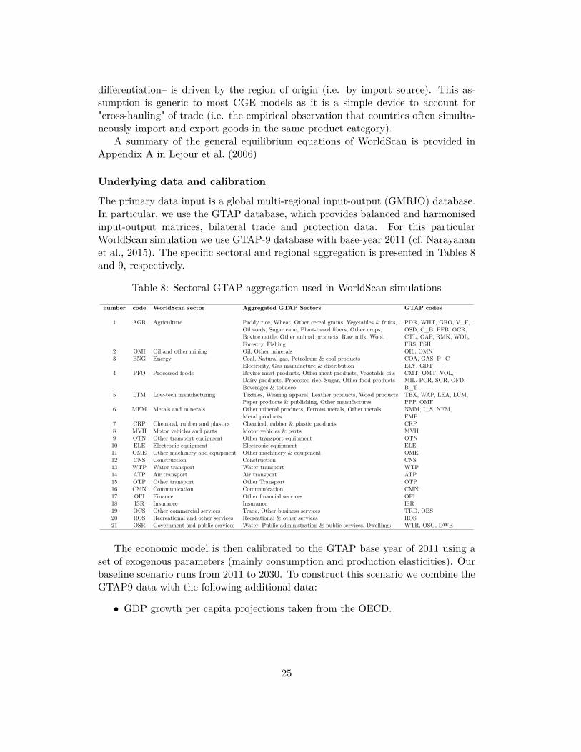
The primary data input is a global multi-regional input-output (GMRIO) database.In particular, we use the GTAP database, which provides balanced and harmonisedinput-output matrices, bilateral trade and protection data. For this particularWorldScan simulation we use GTAP-9 database with base-year 2011 (cf. Narayananet al., 2015). The specific sectoral and regional aggregation is presented in Tables 8and 9, respectively.

Table 8: Sectoral GTAP aggregation used in WorldScan simulations

number code WorldScan sector Aggregated GTAP Sectors GTAP codes

1 AGR Agriculture Paddy rice, Wheat, Other cereal grains, Vegetables & fruits, PDR, WHT, GRO, V_F,Oil seeds, Sugar cane, Plant-based fibers, Other crops, OSD, C_B, PFB, OCR,Bovine cattle, Other animal products, Raw milk, Wool, CTL, OAP, RMK, WOL,Forestry, Fishing FRS, FSH

2 OMI Oil and other mining Oil, Other minerals OIL, OMN3 ENG Energy Coal, Natural gas, Petroleum & coal products COA, GAS, P_C

Electricity, Gas manufacture & distribution ELY, GDT4 PFO Processed foods Bovine meat products, Other meat products, Vegetable oils CMT, OMT, VOL,

Dairy products, Processed rice, Sugar, Other food products MIL, PCR, SGR, OFD,Beverages & tobacco B_T

5 LTM Low-tech manufacturing Textiles, Wearing apparel, Leather products, Wood products TEX, WAP, LEA, LUM,Paper products & publishing, Other manufactures PPP, OMF

6 MEM Metals and minerals Other mineral products, Ferrous metals, Other metals NMM, I_S, NFM,Metal products FMP

7 CRP Chemical, rubber and plastics Chemical, rubber & plastic products CRP8 MVH Motor vehicles and parts Motor vehicles & parts MVH9 OTN Other transport equipment Other transport equipment OTN10 ELE Electronic equipment Electronic equipment ELE11 OME Other machinery and equipment Other machinery & equipment OME12 CNS Construction Construction CNS13 WTP Water transport Water transport WTP14 ATP Air transport Air transport ATP15 OTP Other transport Other Transport OTP16 CMN Communication Communication CMN17 OFI Finance Other financial services OFI18 ISR Insurance Insurance ISR19 OCS Other commercial services Trade, Other business services TRD, OBS20 ROS Recreational and other services Recreational & other services ROS21 OSR Government and public services Water, Public administration & public services, Dwellings WTR, OSG, DWE

The economic model is then calibrated to the GTAP base year of 2011 using aset of exogenous parameters (mainly consumption and production elasticities). Ourbaseline scenario runs from 2011 to 2030. To construct this scenario we combine theGTAP9 data with the following additional data:

∙ GDP growth per capita projections taken from the OECD.

25

Table 9: Regional GTAP aggregation used in WorldScan simulations

Number Code Country/Region description1 AUT Austria2 BAL Baltic countries3 BGR Bulgaria4 BLU Belgium and Luxembourg5 CCM Croatia, Cyprus and Malta6 CZE Czech Republic7 DNK Denmark8 FIN Finland9 FRA France10 DEU Germany11 GRC Greece12 HUN Hungary13 IRL Ireland14 ITA Italy15 NLD Netherlands16 POL Poland17 PRT Portugal18 ROU Romania19 SVK Slovakia20 SVN Slovenia21 ESP Spain22 SWE Sweden23 GBR United Kingdom24 USA United States25 ROE Rest of OECD26 EER Rest of East Europe27 CHH China and Hong Kong28 ASE ASEAN29 IND India30 MNA Middle East and North Africa31 SSA Sub-Saharan Africa32 LAC Latin America and the Caribbean33 ROW Rest of the World

∙ Total labour supply (𝐿𝑆𝑢𝑝) is built using a combination of demographic andlabour data projections, as:

𝐿𝑆𝑢𝑝𝑡 = 𝑃𝑜𝑝𝑡 * 𝑃𝑅𝑡 * (1 − 𝜇𝑡) (1)

where 𝑃𝑜𝑝𝑡 is total population in year 𝑡 with projections taken from theMedium Variant of projections by the United Nations (UN, 2015) (for non-EU countries) and EuroStat population projections for EU countries. Labourparticipation rates (PR) are taken from ILO projections.40 Long-term unem-ployment rates (𝜇) are taken from from EuroStat and World Bank projections.

∙ Trade balances are projected to gradually decrease over time. As an initialbenchmark we use the updated 2011 net foreign assets data from Lane andMilesi-Ferreti (2001).

40From the Economically Active Population Estimates and Projections (EAPEP).

26

The initial (calibrated) condition of the model is that supply and demand arein balance at some equilibrium set of prices and quantities; where workers are sat-isfied with their wages and employment, consumers are satisfied with their basketof goods, producers are satisfied with their input and output quantities and savingsare fully expended on investments. Adjustment to a new equilibrium, governed bybehavioural equations and parameters in the model, are largely driven by price link-age equations that determine economic activity in each product and factor market.For any perturbation to the initial equilibrium, all endogenous variables (i.e. pricesand quantities) adjust simultaneously until the economy reaches a new equilibrium.Constraints on the adjustment to a new equilibrium include a suit of accounting re-lationships that dictate that in aggregate, the supply of goods equals the demand forgoods, total exports equals total imports, all (available) workers and capital stock isemployed, and global savings equals global investment; unless adjustments to theseassumptions are modified for a particular application.

A.2 TTIP simulations with different NTB reductions

Table 10 presents the main macroeconomic results of TTIP with different NTBreductions than those presented in the main scenario (Table 4). We observe thatthere is a quasi-linear relation between NTB cuts and GDP gains: i.e. reducing theNTB reductions by half, also reduced the GDP gains by roughly half.

Table 10: TTIP simulation results using different NTB reductions, percentagechanges with respect to the baseline in 2030

Full TTIP 50% NTB reduction 25% NTB reductionNLD EU28 USA NLD EU28 USA NLD EU28 USA

GDP 1.69 1.19 0.94 0.81 0.59 0.55 0.39 0.30 0.33consumption per capita 3.11 2.16 1.93 1.33 0.89 0.86 0.61 0.41 0.44export volume 3.94 6.24 21.45 1.80 2.81 9.95 0.94 1.47 5.33import volume 7.50 8.99 23.85 3.11 3.70 10.16 1.51 1.82 5.12real average wage 2.13 1.66 1.59 0.91 0.68 0.73 0.42 0.32 0.39

Notes: The 50 and 25% NTB reduction are relative to the NTB reductions in the full TTIPscenario.Source: Own WorldScan estimations using GTAP9 database.

27

Publisher:

CPB Netherlands Bureau for Economic Policy AnalysisP.O. Box 80510 | 2508 GM The Haguet (070) 3383 380

July 2016 | ISBN 978-90-5833-738-2