Potential Anthropogenic Pollution of High-technology ...
40
1 Reviews 1 Potential Anthropogenic Pollution of High-technology 2 Metals with a Focus on Rare Earth Elements in 3 Environmental Water 4 5 Akihide ITOH,* , † Akane YAIDA,** and Yanbei ZHU*** 6 7 * Department of Environmental Science, School of Life and Environmental Science, 8 Azabu University, 1-17-71 Fuchinobe, Chuo-ku, Sagamihara, Kanagawa 252-5201, 9 Japan 10 ** Graduate School of Environmental Health Sciences, Azabu University, 1-17-71 11 Fuchinobe, Chuo-ku, Sagamihara, Kanagawa 252-5201, Japan 12 *** National Metrology Institute of Japan (NMIJ), National Institute of Advanced 13 Industrial Science and Technology (AIST), 1-1-1 Umezono, Tsukuba, Ibaraki 305- 14 8563, Japan 15 16 Contents 17 1. Introduction 18 2. REEs in environmental water 19 2.1 Analytical methods 20 2.2 REE concentration anomalies 21 2.3 Comparison of the degree of Gd anomalies 22 2.4 Chemical speciation of Gd compounds 23 2.5 Ecotoxicology and bioavailability of anthropogenic REEs 24 3. Multielement analysis of high technology metals as well as REEs 25 4. Conclusion 26 5. Acknowledgements 27 6. References 28 29 † To whom correspondence should be addressed. 30 E-mail: [email protected] 31 32 Analytical Sciences Advance Publication by J-STAGE Received September 19, 2020; Accepted November 2, 2020; Published online on November 6, 2020 DOI: 10.2116/analsci.20SAR16
Transcript of Potential Anthropogenic Pollution of High-technology ...
1
Reviews 1
Potential Anthropogenic Pollution of High-technology 2
Metals with a Focus on Rare Earth Elements in 3
Environmental Water 4
5
Akihide ITOH,*, † Akane YAIDA,** and Yanbei ZHU*** 6
7
* Department of Environmental Science, School of Life and Environmental Science,8
Azabu University, 1-17-71 Fuchinobe, Chuo-ku, Sagamihara, Kanagawa 252-5201,9
Japan10
** Graduate School of Environmental Health Sciences, Azabu University, 1-17-71 11
Fuchinobe, Chuo-ku, Sagamihara, Kanagawa 252-5201, Japan 12
*** National Metrology Institute of Japan (NMIJ), National Institute of Advanced 13
Industrial Science and Technology (AIST), 1-1-1 Umezono, Tsukuba, Ibaraki 305-14
8563, Japan 15
16
Contents 17
1. Introduction18
2. REEs in environmental water19
2.1 Analytical methods 20
2.2 REE concentration anomalies 21
2.3 Comparison of the degree of Gd anomalies 22
2.4 Chemical speciation of Gd compounds 23
2.5 Ecotoxicology and bioavailability of anthropogenic REEs 24
3. Multielement analysis of high technology metals as well as REEs25
4. Conclusion26
5. Acknowledgements27
6. References28
29
† To whom correspondence should be addressed. 30
E-mail: [email protected]
32
Analytical SciencesAdvance Publication by J-STAGEReceived September 19, 2020; Accepted November 2, 2020; Published online on November 6, 2020DOI: 10.2116/analsci.20SAR16

2
Abstract 33
34
In recent years, utilization of high technology metals such as rare earth elements 35
(REEs), whose abundance are extremely low in the earth, has rapidly increased with 36
development of new types of industrial materials and pharmaceutical products. This 37
review overviews a new type of potential anthropogenic pollution of the high-technology 38
metals with a focus on REEs released in environmental water from a waste treatment 39
facility. In this paper, potential anthropogenic pollution was defined as pollution caused 40
by metals gradually enriched in the environment by human activity, although standard 41
and guideline concentrations of these elements are not regulated by environmental quality 42
standards for water pollution. We review the analytical methods of REEs and the potential 43
anthropogenic pollution of REEs with a focus on Gd in the viewpoints of comparison of 44
degree of Gd anomaly, chemical speciation, ecotoxicology, and bioaccessibility. 45
Moreover, we also highlight the comprehensive analysis based on multielement analysis 46
of high technology metals as well as REEs for the further screening of a potential 47
anthropogenic pollution. 48
49
50
Key words: ICP-MS; trace metal, REEs; Gadolinium, river water; coastal seawater; 51
ecotoxicology; bioaccessibility; speciation; concentration anomaly. 52
53
54
55
56
57
58
Analytical SciencesAdvance Publication by J-STAGEReceived September 19, 2020; Accepted November 2, 2020; Published online on November 6, 2020DOI: 10.2116/analsci.20SAR16

3
1. Introduction 59
The presence of excessive heavy metals in the environment has negatively affected 60
the health of humans, animals, and plants. Hence, at present, in a general water quality 61
investigation of the environmental, the concentrations of many trace metals in 62
environmental water are controlled to monitor its quality as well as to protect human 63
health and/or aquatic life.1-3 For example, in Japan, Cd, Pb, Cr(VI), As, Hg (total and 64
alkyl-), Se, Ni, Mo, Sb, Mn, and U are regulated in the Environmental Quality Standards 65
for Water Pollution of Japan,1 while Al, Sb, As, Ba, Be, Cd, Cr (III and VI), Cu, Fe, Pb, 66
Mn, Hg (total and methyl-), Ni, Se, Ag, Tl, Sn (tributyltin) and Zinc are regulated in the 67
National Recommended Water Quality Criteria of the United States of America.2,3 Many 68
studies concerning the analysis of these elements have been reported.4-11 The 69
concentrations required for regulation are generally at mg L-1 to μg L-1 levels, and their 70
determination can be accomplished using inductively coupled plasma mass spectrometry 71
(ICP-MS), inductively coupled plasma optical emission spectrometry (ICP-OES), and 72
atomic absorption spectrometry (AAS). Various studies for heavy metals in 73
environmental waters such as rivers, lakes, and coastal seawater has been performed not 74
only for concentration,12-26 but also for speciation,27-29 environmental toxicology,30-34 and 75
assessment of aquatic ecosystem.35-37 76
In recent years, utilization of high technology metals such as rare earth elements 77
(REEs), whose abundance are extremely low in the earth, has rapidly increased with 78
development of new types of industrial materials and pharmaceutical products.38,39 In 79
Japan, the Ministry of Economy, Trade and Industry, defined these elements as “rare 80
metal”. 40 These include 31 mineral species and 47 elements. If materials including these 81
elements were disposed without appropriate control, a new type of environmental 82
Analytical SciencesAdvance Publication by J-STAGEReceived September 19, 2020; Accepted November 2, 2020; Published online on November 6, 2020DOI: 10.2116/analsci.20SAR16

4
pollution may occur. Thus, we became interested in the research for a new type of 83
potential anthropogenic pollution of high-technology metals with a focus on REEs in 84
environmental water. In this paper, potential anthropogenic pollution was defined as 85
pollution caused by metals gradually enriched in the environment by human activity, 86
although standard and guideline concentrations of these elements are not regulated by 87
environmental quality standards for water pollution. In particular, many researches for 88
anthropogenic REEs in environmental water have been reported worldwide. The 89
significant increase in the use of REEs in high technology products and processes has led 90
to an increased release of these metals into the environment. Hence, the determination of 91
REEs in the environment have been performed not only from the viewpoint of 92
geochemistry and geoscience, but also from the environmental concern. The first report 93
of the anthropogenic REEs in the environmental water was published in 1996,41 when the 94
concentration anomaly of Gd was identified in the Havel River in Germany. Nowadays, 95
it is widely known that the relative abundance of Gd in the river water and coastal 96
seawater around large metropolitan areas is typically higher than those of its neighboring 97
REEs, i.e. Eu and Tb.15,39,41-64 This was artificially caused by anthropogenic sources 98
mainly due to use of Gd compounds used as a contrast reagent for magnetic resonance 99
imaging (MRI) in medical diagnosis. 100
In this paper, we review the analytical methods of REEs and the potential 101
anthropogenic pollution of REEs with a focus on Gd in the viewpoints of comparison of 102
degree of Gd anomaly, chemical speciation, ecotoxicology, and bioaccessibility. 103
Moreover, we also highlight the comprehensive analysis based on multielement analysis 104
of high technology metals as well as REEs for the further screening of a potential 105
anthropogenic pollution. 106
Analytical SciencesAdvance Publication by J-STAGEReceived September 19, 2020; Accepted November 2, 2020; Published online on November 6, 2020DOI: 10.2116/analsci.20SAR16
5
107
2. REEs in environmental water 108
2.1 Analytical methods 109
Nowadays, ICP-MS is the dominating approach for the determination of REEs in 110
environmental water.43, 49, 50, 65-96 Other works reported the determination of REEs using 111
neutron activation analysis (NAA)97,98 and thermal ionization mass spectrometry 112
(TIMS).51,99,100 The increasing application of ICP-MS in the determination of REEs can 113
be attributed to increasing availability of ICP-MS in the laboratories for analysis, as well 114
as to the capability of ICP-MS for simultaneous determination of REEs at pg mL-1 level. 115
A comparison of analytical performance of ICP-MS-based techniques for 116
determination of REEs in environmental water is summarized in Table 1. As can be seen 117
from Table 1, the lowest value of detection limit obtained by direct measurement with 118
ICP-MS varied from 0.003 pg mL-1 for Tm to 1.9 pg mL-1 for Dy.49,75,76, 78, 85 The detection 119
limits would depend both on the model of ICP-MS instrument and on the operating 120
conditions. A sample volume not more than 10 mL can be processed for the determination 121
of REEs by ICP-MS when a preconcentration factor under 10-fold is enough.49,77 A 122
preconcentration factor more than 30-fold are usually obtained with a sample volume 123
from 40 to 5000 mL.66,-69, 80, 81, 90, 94-96 The lowest value of detection limit reported for 124
REEs determined by ICP-MS varied from 0.001 pg mL-1 to approximately 2 pg mL-1. The 125
reported analytical performances in Table 1 might indicate that the lowest value of 126
detection limit for measurement of REEs in environmental water by ICP-MS with 127
preconcentration depends on both the operating conditions and the pretreatment 128
techniques.49, 65- 71, 73, 75-78, 80, 81, 85 90, 94-96 129
In order to evaluate the anomaly of some REEs, scientists often attempt to determine 130
the whole group of REEs instead of selected ones that can be determined directly with 131
Analytical SciencesAdvance Publication by J-STAGEReceived September 19, 2020; Accepted November 2, 2020; Published online on November 6, 2020DOI: 10.2116/analsci.20SAR16

6
ICP-MS. However, in this case, some REEs are often near or below the detection limit 132
of an ICP-MS instrument. Consequently, preconcentration of REEs must be carried out 133
prior to the ICP-MS measurement. In addition, removal of high contents of salt (ca. 3.5 %) 134
is often required for measuring REEs in seawater samples so as to reduce the burden to 135
the introduction system (e.g., torch, cones, and ion-lens, etc.) of an ICP-MS instrument. 136
There are multiple approaches reported for the preconcentration of REEs prior to the 137
measurement, including coprecipitation with Fe(OH)3,51, 65, 95, 100 coprecipitation with 138
Mg(OH)2,81 solid phase extraction (SPE) with chelating resin, 67, 69, 70, 72, 80, 87, 89, 93, 96-97 139
cation exchange,71 chromatography,73,74 solvent extraction,78 magnetic SPE with 140
nanoparticles,90 and extraction with calcium alginate microparticles.94 141
The majority of studies employed the SPE with chelating resins for 142
preconcentration of REEs prior to the measurement by ICP-MS. It can be attributed to 143
the merits of the good selection for REEs without introduction of a new metal-matrix as 144
well as the relatively simpler operations than cation exchange. Laboratory-modified C18 145
cartridge, on which the complexing agent composed of a mixture of bis(2-ethylhexyl) 146
dihydrogen phosphate (HDEHP) and 2-ethylhexyl dihydrogen phosphate (H2MEHP) was 147
loaded, was also reported as an effective SPE for preconcentration of REEs in seawater 148
samples.66 This preconcentration method was either performed by utilizing the complex 149
formation between REEs and chelating resin or reagent. They have often been applied to 150
the determination of all REEs in environmental water including seawater by many 151
research groups to investigate the concentration anomalies.41, 42, 44-46, 48 However, due to 152
increasing availability of commercial chelating resins, in recent years, they become a 153
popular choice for SPE processes and concentration of REEs. 154
It is remarkable that the presence of organic compounds (e.g., 155
Analytical SciencesAdvance Publication by J-STAGEReceived September 19, 2020; Accepted November 2, 2020; Published online on November 6, 2020DOI: 10.2116/analsci.20SAR16

7
ethylenediaminetriacetic acid at nmol L-1 level) in environmental water samples affects 156
the recovery of REEs during the preconcentration process involving the complex 157
formation of REEs,47, 96 despite acidification of filtered water samples to pH 1 by the 158
addition of HNO3 or HCl. The reason for this phenomenon can be attributed to the 159
competition between refractory organic anions and functional groups of chelating resin 160
(e.g., carboxyl group) and reagents in adsorbing of REEs in environmental water samples. 161
Hence, decomposition of organic compounds by acid treatment with HNO3 and H2O2 at 162
170 ℃ for 4 h was proposed prior to the SPE operation with chelating resin to improve 163
the recovery of REEs.96 164
Polyatomic spectral interferences must also be considered for accurate determination 165
of REEs by ICP-MS. Typical polyatomic spectral interferences are summarized in Table 166
S1. Typical polyatomic spectral interferences and the resolution required for separation 167
in Table S1 are estimated from the isotopic mass of each element.102 In most of the 168
reported works, corrections of such polyatomic spectral interferences were carried out 169
based on mathematic calculations of the production rates of these interfering species. It 170
is notable that the removal of Ba from the sample during the preconcentration process for 171
REEs helps to reduce spectral polyatomic interferences with the measurement of 139La 172
(138Ba1H) and 151Eu(135Ba16O), and 153Eu (137Ba16O). This is especially important because 173
the concentration of Ba in environmental water samples is usually much higher than those 174
of La and Eu by three-to-four orders of magnitudes. Thus, spectral interferences can be 175
problematic, even if the ICP-MS measurement is performed under beneficial conditions 176
of very low ratio of BaH+/Ba+ and BaO+/Ba+. 177
Fortunately, the availability of tandem quadrupole ICP-MS with a reaction cell (also 178
known as ICP-QQQ) permitted the complete separation of polyatomic spectral 179
Analytical SciencesAdvance Publication by J-STAGEReceived September 19, 2020; Accepted November 2, 2020; Published online on November 6, 2020DOI: 10.2116/analsci.20SAR16

8
interferences from isotopes of REEs by using oxygen as the reaction gas and measuring 180
the REEs as their mono-oxide ions.103 In the near future, there may be more applications 181
by this type of ICP-MS instrument to the determination of REEs in environmental water. 182
The precision for the results of REEs might depend on the instrument for 183
determination, preconcentration technique, and preconcentration factor. When the 184
concentrations of REEs in the measured solutions are sufficient for determination, a 185
typical relative standard deviation around 1% to 5% can be achieved.66, 76, 96 Such 186
precision is no problem for the evaluation of anomalies of REEs in natural water samples, 187
because the concentration anomalies in the REE patterns are often illustrated as logarithm 188
scale. Isotope dilution analysis had also been reported for the determination of REEs in 189
natural water samples and contributed to improving the accuracy of the results with 190
precisions comparable to those obtained by calibration curve methods.104, 105 The 191
application of multi-collector (MC-) ICP-MS to isotope dilution analysis of REEs might 192
help to improve the precision of measurement. However, there is few reports about 193
concentrations of REEs in natural water obtained by isotope dilution MC-ICP-MS, 194
Moreover, it is difficult to investigate concentration anomalies of REEs using the isotope 195
dilution-ICP-MS, because mononuclidic REEs such as Pr, Tb, Ho, and Tm can not be 196
determined. Procedure blank values for the determination of REEs in natural water are 197
usually controlled at a sufficiently lower level in comparison to those in the samples. 198
199
2.2 Concentration anomaly of REEs 200
It is widely known that the concentration distributions of REEs in environmental 201
water typically show zig-zag patterns, according to the Oddo-Harkins rule.106 This 202
indicates that the concentration of REEs with even atomic numbers are higher than those 203
of the neighboring REEs with odd atomic numbers. Thus, REE patterns, normalized by 204
Analytical SciencesAdvance Publication by J-STAGEReceived September 19, 2020; Accepted November 2, 2020; Published online on November 6, 2020DOI: 10.2116/analsci.20SAR16
9
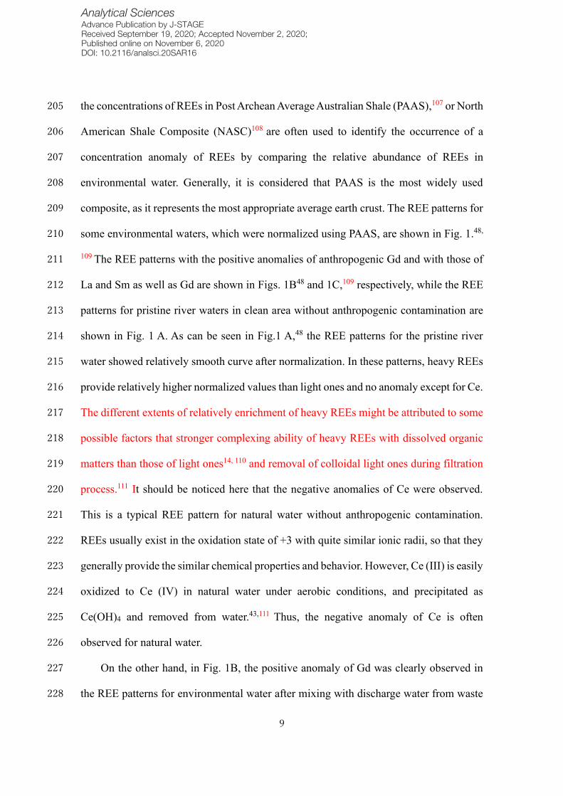
the concentrations of REEs in Post Archean Average Australian Shale (PAAS),107 or North 205
American Shale Composite (NASC)108 are often used to identify the occurrence of a 206
concentration anomaly of REEs by comparing the relative abundance of REEs in 207
environmental water. Generally, it is considered that PAAS is the most widely used 208
composite, as it represents the most appropriate average earth crust. The REE patterns for 209
some environmental waters, which were normalized using PAAS, are shown in Fig. 1.48, 210
109 The REE patterns with the positive anomalies of anthropogenic Gd and with those of 211
La and Sm as well as Gd are shown in Figs. 1B48 and 1C,109 respectively, while the REE 212
patterns for pristine river waters in clean area without anthropogenic contamination are 213
shown in Fig. 1 A. As can be seen in Fig.1 A,48 the REE patterns for the pristine river 214
water showed relatively smooth curve after normalization. In these patterns, heavy REEs 215
provide relatively higher normalized values than light ones and no anomaly except for Ce. 216
The different extents of relatively enrichment of heavy REEs might be attributed to some 217
possible factors that stronger complexing ability of heavy REEs with dissolved organic 218
matters than those of light ones14, 110 and removal of colloidal light ones during filtration 219
process.111 It should be noticed here that the negative anomalies of Ce were observed. 220
This is a typical REE pattern for natural water without anthropogenic contamination. 221
REEs usually exist in the oxidation state of +3 with quite similar ionic radii, so that they 222
generally provide the similar chemical properties and behavior. However, Ce (III) is easily 223
oxidized to Ce (IV) in natural water under aerobic conditions, and precipitated as 224
Ce(OH)4 and removed from water.43,111 Thus, the negative anomaly of Ce is often 225
observed for natural water. 226
On the other hand, in Fig. 1B, the positive anomaly of Gd was clearly observed in 227
the REE patterns for environmental water after mixing with discharge water from waste 228
Analytical SciencesAdvance Publication by J-STAGEReceived September 19, 2020; Accepted November 2, 2020; Published online on November 6, 2020DOI: 10.2116/analsci.20SAR16

10
treatment facility (WWTF). It is well known that this was caused by environmental 229
outflow of Gd compounds used as contrast reagent for MRI in medical diagnosis, 230
although Gd is also used as the manufacture and polishing of glass products, the 231
phosphors in computer monitor, and color television tubes and the nuclear reactor control 232
rod etc. The Gd compounds are administrated to patients in a hospital and are then 233
excreted as waste and transported into environmental water via WWTP. They are directly 234
released into river water from the discharging water without eliminating during the waste 235
treatment process in WWTF. Consequently, Gd anomalies were observed in 236
environmental water around large metropolitan area. The concentration anomalies due to 237
the anthropogenic Gd have been reported for all kind of environmental waters including 238
river waters, lake waters, groundwater, and coastal seawater all over the world since the 239
mid-1990s.41-64 In addition, the Gd anomalies in the REE patterns were observed in tap 240
water sampled in Berlin along the Havel River and other German cities along the Rhine 241
River as well as in the environmental water.107 The anthropogenic Gd was also found in 242
tap water and tap water-based beverages from fast-food franchises in six major Germany 243
cities.108 244
In recent years, the positive concentration anomalies of La, Sm, Ce, Eu as well as Gd 245
have been reported.109, 112 The occurrence of a positive Ce anomaly is influenced by its 246
redox state in the environmental water; therefore, it is not necessarily caused by 247
anthropogenic micro-contamination. However, other anomalies for REEs would be 248
caused by anthropogenic micro-contaminant. As shown in Fig. 1C, Kulaksiz and Bau109 249
reported that anthropogenic Sm and La as well as anthropogenic Gd was detected in the 250
Rhine River near the border between Germany and the Netherlands. Based on analysis 251
using ultrafiltration, it is suggested that while the anthropogenic Gd is not particle-252
Analytical SciencesAdvance Publication by J-STAGEReceived September 19, 2020; Accepted November 2, 2020; Published online on November 6, 2020DOI: 10.2116/analsci.20SAR16

11
reactive and thus exclusively present in the truly dissolved REE fraction (<10 kDa), the 253
anthropogenic La and Sm are present in the colloidal/nanoparticulate REE fraction (10 254
kDa-0.2 m). Although the origin of Sm was unclear, it is considered that La was derived 255
from a point source where industrial cracking catalysts for petroleum refining were 256
produced. However, there is no obvious reason why chemical speciation of Sm should 257
differ from that of anthropogenic La. Their analytical results indicate that anthropogenic 258
Sm might originate from the same industrial cracking catalyst production effluent that 259
causes the La positive anomaly. Sm compounds are utilized in a high-strength permanent 260
magnet to control rods in nuclear reactors. They are also employed as catalysts in the 261
decomposition of plastics, dichlorination of polychlorinated biphenyls (PCBs), and 262
dehydration and dehydrogenation of ethanol. Furthermore, SmI2 is commonly used as 263
reducing and coupling reagents in organic synthesis. On the other hand, as it can be seen 264
from Fig. 1 C, positive anomaly of Pr as well as Gd, La, and Sm was observed in the 265
samples form the industrial cracking catalyst production effluent pipe at Rhine River. 266
However, this was not mentioned in the report by Kulaksiz and Bau.109 267
The Eu anomaly can be caused by the presence of Eu-enriched minerals in the 268
vicinity of environmental water and/or the result of the unique redox behavior. 269
Specifically, Eu3+ can be reduced to Eu2+, which exhibits increased solubility. The 270
reduction of this element occurs more readily than it does in the case of other REEs. Thus, 271
the anomaly of Eu due to naturally-occurring Eu were often observed in the samples from 272
the upstream river water to estuarine water.113 On the other hand, when the river water 273
samples are measured in the quadrupole ICP-MS, 151Eu and 153Eu is often interfered with 274
135Ba16O and 137Ba16O formed at the relatively high concentration of Ba in the samples. 275
Hence, in the case of direct ICP-MS measurement, the Eu anomaly has sometimes been 276
Analytical SciencesAdvance Publication by J-STAGEReceived September 19, 2020; Accepted November 2, 2020; Published online on November 6, 2020DOI: 10.2116/analsci.20SAR16

12
observed in the REE patterns as a result of spectral interference. In contrast, Itoh et al. 277
reported that the concentration anomaly of anthropogenic Eu in the Sakai-River was 278
caused by the effluent of a specific WWTF, even after the removal of a large proportion 279
of Ba by SPE with chelating resin and correction by spectral interference coefficient 280
method.112 Nowadays, the main origin of Eu is unknown, although Eu is used in liquid 281
crystal displays, fluorescent lighting, glass additives etc. 282
283
2.3 Comparison of the degree of Gd anomalies 284
To compare the Gd concentrations in samples from various environmental waters 285
around the world, it is important that the degree of the positive anthropogenic Gd 286
anomaly is objectively evaluated. However, when such comparisons are made, it should 287
be considered that the Gd concentrations are influenced by rainfall or naturally-288
occurring REEs in rocks and soils in the vicinity of the river water. Thus, a conversion 289
of the positive Gd anomaly into numerals is performed for each REE pattern using two 290
indexes. One index is the Panomaly (%), which indicates the percentages of the 291
anthropogenic Gd to the naturally-occurring one. It was defined by Zhu et al.43 and Yaida 292
et al.47 using the following equation (1): 293
𝑃anomaly = GdSN−GdSN∗
GdSN∗× 100(%) (1) 294
where GdSN is the shale (PAAS)-normalized concentration of Gd observed in 295
environmental water, and GdSN* is the theoretical shale-normalized concentration of Gd 296
when the positive anomaly is not observed in the REE patterns. GdSN* is approximated 297
from the straight line obtained from PAAS-normalized concentrations of Sm, Tb, and Dy 298
using the least square method. When Panomaly shows higher values (i.e., > 100%), it 299
suggested that the contribution rate of anthropogenic Gd to naturally occurring Gd is 300
Analytical SciencesAdvance Publication by J-STAGEReceived September 19, 2020; Accepted November 2, 2020; Published online on November 6, 2020DOI: 10.2116/analsci.20SAR16

13
larger. 301
Another index is GdSN/GdSN*, which was defined by the first reports for the positive 302
Gd anomalies in river waters by Bau and Dulski using the following equation (2) 303
GdSN/Gd*SN = GdSN/(0.33Sm SN + 0.67TbSN) (2) 304
However, Gd*SN was often estimated by employing other extrapolation methods. For 305
example, Kulaksiz and Bau proposed that Gd*SN was extrapolated using the shale-306
normalized values of Pr, Nd, and Sm in the REE pattern. In any case, a value of 307
GdSN/Gd*SN larger than 1.0 indicates the presence of an anthropogenic Gd in the 308
environmental water. 309
The Gd concentration and GdSN/Gd*SN index for natural land water, such as river 310
water, and for seawater samples obtained in various parts of the world are summarized in 311
Tables 2 and 3, respectively. The values of GdSN/Gd*SN were estimated from the 312
previously reported analytical data. Gd*SN was extrapolated using the shale-normalized 313
values of Sm, Tb, and Dy. It is noteworthy that the Panomaly and GdSN/Gd*SN index are 314
similar. The former is calculated by subtracting 1 from the value of GdSN/Gd*SN and 315
multiplying by 100. GdSN/Gd*SN was employed as the index in Tables 2 and 3, in which 316
the highest Gd concentrations were shown when several Gd concentrations were reported 317
for the same environmental waters. The GdSN/Gd*SN index values is considered to show 318
objectively the degree of Gd anomalies to some extent, while they are governed by the 319
mixing ratio of the river water and the discharge water from WWTF. In Tables 2 and 3, 320
the data for each natural land water and seawater are arranged in descending order of the 321
GdSN/Gd*SN index values. 322
As can be seen in Table 2, many studies on the Gd anomaly in natural land waters 323
such as river waters, have been reported so far. The reported concentrations of Gd ranged 324
Analytical SciencesAdvance Publication by J-STAGEReceived September 19, 2020; Accepted November 2, 2020; Published online on November 6, 2020DOI: 10.2116/analsci.20SAR16

14
from 1 ng L-1 to several hundred ng L-1. In addition, the GdSN/Gd*SN index ranged from 325
1.1 to more than 2.0 in large metropolitan areas. This indicates that some parts of Gd 326
dissolved in natural land water have the anthropogenic origin, even in river water in the 327
suburb area. The Gd concentration and the GdSN/Gd*SN index in Havel River (Germany) 328
in 2009 were 492 ng L-1 and 653, respectively. Notably, these were the highest values 329
among all reported for natural land waters. This data indicates that the concentration of 330
anthropogenic Gd were more than 650-fold higher than the concentration of naturally-331
occurring Gd in the Haver River in 2009. Especially, larger values of GdSN/Gd*SN over 332
10 were seen in the river water samples in Germany, Japan, Brazil, and Poland. Most of 333
these reports was published after 2010. Incidentally, the owned number of MRI was in 334
order of the United States, Japan, and Germany. 335
On the other hand, the concentrations and the index values for the seawater were shown 336
in Table 3. As can be seen in Table 3, the Gd concentrations for seawater are generally 337
lower than those for natural land water, even in coastal seawater. This is because their Gd 338
concentrations were diluted by large amounts of seawater. The Gd concentration and 339
GdSN/Gd*SN index value were the highest for the coastal seawater in Tokyo Bay in 2008 340
among all reports. The Gd concentration and GdSN/Gd*SN index obtained from the same 341
sampling sites reported more than twice in different years are summarized in Table 4. As 342
can be seen in Table 4, for the Havel, Rhine, Elbe, and Tama Rivers as well as for the San 343
Francisco and Tokyo Bays, the values of the Gd concentration and GdSN/Gd*SN obtained 344
in recent years are larger than those determined in the past. Hence, it is suggested that 345
degree of Gd anomaly has been increasing annually in most of environmental water. 346
It is considered that the ecotoxicological effects would be not so high because the Gd 347
concentration level is very low under 1 g L-1, even in the Havel River showing the 348
Analytical SciencesAdvance Publication by J-STAGEReceived September 19, 2020; Accepted November 2, 2020; Published online on November 6, 2020DOI: 10.2116/analsci.20SAR16
15
highest value. Nevertheless, considering that the concentrations of anthropogenic Gd 349
have been gradually increasing in many river waters and coastal seawaters, environmental 350
monitoring must be performed to assess the risk to the aquatic ecosystem and human 351
health. 352
353
2.4 Chemical speciation of Gd compounds 354
It is important to elucidate the chemical species of Gd as well as the total Gd 355
concentration to investigate the ecotoxicological influences of the anthropogenic Gd on 356
the aquatic animals and plants and to assess its risk to human health. To evaluate the 357
chemical speciation of Gd in environmental water, the separation of Gd compounds used 358
as the contrast agents were attempted employing various analytical methods. However, 359
this process is extremely challenging due to the low concentrations of such species. The 360
main Gd compounds used as the contrast agent of MRI, which are all Gd complexes, are 361
summarized in Fig. 2.114 362
The hyphenation of separation techniques such as HPLC with ICP-MS have been 363
employed for speciation analysis of Gd in the environmental water.114-121 The ion 364
chromatography (IC)115 and the size exclusion chromatography (SEC)116, 117 were used as 365
separation method to separate Gd compounds used as the contrast agents and the Gd3+, 366
which is the most toxic species. In the IC/ICP-MS, Gd-DTPA (Magnevist) and Gd3+ could 367
be separated using the cation exchange separation column. The SEC/ICP-MS enabled the 368
separation of several Gd complexes and Gd3+ to some extent. Nevertheless, the 369
differences in the sizes of Gd complexes are too small for efficient SEC separation. On 370
the other hand, a hyphenation of hydrophilic interaction liquid chromatography (HILIC) 371
and ICP-MS has been employed as highly sensitive method for speciation analysis of 372
several Gd-based contrast agents in hospital effluents, river waters, WWTP effluents and 373
Analytical SciencesAdvance Publication by J-STAGEReceived September 19, 2020; Accepted November 2, 2020; Published online on November 6, 2020DOI: 10.2116/analsci.20SAR16

16
tap water. Birka et al. reported the sensitive quantification of the Gd-based contrast 374
reagents in river water samples using HILIC/ICP-MS.118-120 In their studies, this river 375
water sample was collected from a nature reserve in the city of Münster in Germany, 376
where the effluent from the city’s main WWTP enters the environment. Three kinds of 377
contrast agents, namely Gd-DTPA, Gd-DOTA (Dotarem) and Gd-BT-DO3A (Gadovist), 378
were identified and quantified in the obtained samples. The concentrations ranged from 379
0.59 nmol L-1 for Gd-DOTA up to 3.55 nmol L-1 for Gd-BT-DO3A. As a result of mass 380
balancing, the concentration of the Gd-based contrast agents was found to account for 74-381
89% of the total Gd concentration, thus indicating the presence of other Gd species. 382
Lindner et al. used a new zwitterionic HILIC column (ZIC-cHILIC) for speciation of Gd-383
containing contrast agents in tap water.120 ZIC-cHILIC contained a phosphorylcholine 384
moiety instead of a sulfobetaine group on the ZIC-HILIC. The positively charged head 385
group of the phosphorylcholine functionality in ZIC-cHILIC produced more surface 386
charges, which could interact with the negatively charged contrast agents more efficiently. 387
Overall, the more effective separation of negatively charged Gd-based contrast agents 388
from the new stationary phase was performed using ZIC-cHILIC. ZIC-cHILIC-ICP-MS 389
makes it possible to separate and determine the five contrast agents, i.e., Gd-BOPTA 390
(Multhiance), GD-DTPA, Gd-DOTA, Gd-DTPA-BMA (Omniscan), and Gd-BT-DO3A. 391
The chromatogram for Gd compounds in tap water samples obtained in Berlin (Germany) 392
measured by ZIC-cHILIC-ICP-MS are illustrated in Fig. 3. As shown in Fig. 3, three Gd 393
species, specifically Gd-BT-DO3A, Gd-DOTA and Gd-BOPTA, were found in tap water 394
samples at concentrations of approximately 10-20 ng L-1. It is noteworthy that these were 395
the same Gd species that had been previously detected in the surface waters, such as rivers 396
and lakes, in the western part of Berlin.45 This implies that the contrast agents were 397
Analytical SciencesAdvance Publication by J-STAGEReceived September 19, 2020; Accepted November 2, 2020; Published online on November 6, 2020DOI: 10.2116/analsci.20SAR16

17
transported from the surface waters through the bank filtration water into the tap; 398
therefore, it is possible that they entered the food chain. 399
400
2.5 Ecotoxicology and bioaccessibility of anthropogenic REEs 401
As described in Section 2.3, recent studies have showed that the concentrations of 402
Gd and some other REEs levels continue to increase in the environmental water and/or in 403
tap water. Nonetheless, their ecotoxicological effects as well as their influence on the 404
aquatic life and human health remain poorly understood. REEs are considered of minor 405
environmental concern due to their low toxicity to mammals.34 Although REEs have 406
received attention as environmental micro-contaminant in recent years, little is known 407
about their influences on aquatic organisms. Despite being considered as safe for many 408
years, in 2006, it was found that administration of Gd-based contrast agents led to serious 409
side effects, nephrogenic systemic fibrosis (NSF).122 It is speculated that the toxicity of 410
Gd-based contrast agents was predominantly caused by Gd3+ dissociated from them. The 411
ionic radius of Gd3+ is roughly equal to Ca2+, resulting in the blockage of the calcium ion 412
channels in the cells.64 Moreover, Gd3+ regularly binds with a higher affinity than Ca2+ 413
and completes with it during physiological processes.39 Hence, it is essential to further 414
investigate the bioaccessibility and ecotoxicological impact of anthropogenic REEs. 415
Studies on bioaccumulation and bioaccessibility of REEs have been performed mainly 416
using fishes, bivalves and algae.34 In this review, we introduce the studies using bivalves 417
for assessment of the influences of REEs on aquatic organism. 418
Merschel and Bau examined the bioaccessibility of anthropogenic La, Sm, and Gd in 419
river water by analyzing the aragonitic shell of freshwater mussel Corbicula fluminea.123 420
The shale (PAAS)- normalized REE patterns for Corbicula fluminea is illustrated in Fig. 421
Analytical SciencesAdvance Publication by J-STAGEReceived September 19, 2020; Accepted November 2, 2020; Published online on November 6, 2020DOI: 10.2116/analsci.20SAR16

18
4. The results in Fig. 4B indicate that all shells sampled at sites downstream of the 422
industrial point source of anthropogenic La and Sm in the Rhine River (at Worms) show 423
the positive La and Sm anomalies (the industrial point source of anthropogenic Sm was 424
situated only at Leverkusen). On the other hand, anomalous enrichment of Gd was not 425
observed in any of the analyzed shells. Hence, it was suggested that anthropogenic La 426
and Sm, which were detected in tap water as well as in river water, are bioaccessible. In 427
contrast, the anthropogenic Gd was not incorporated into the shells. The outcomes 428
regarding the incorporation of anthropogenic Gd in the Corbicula fluminea shells were 429
consistent with previous evidence concerning the long environmental half-life of Gd-430
based compounds used as contrast agents. Additionally, the results of this study further 431
implied that the conservative behavior of anthropogenic Gd makes it a useful tracer of 432
WWTP effluent mixed in river, lake, ground and tap waters. It is noticeable that the PAAS 433
normalized REE patterns of shells showed apparently relative depletion of heavy REEs 434
in comparison to those of water samples plotted in Fig. 1. This characteristic of PAAS 435
normalized REE patterns of shells might reflect the initial components of REEs in 436
particulates taken by the Corbicula fluminea or more favorable intake of heavy REEs 437
than light ones during the shell formation process. 438
On the other hand, Perrat et al. investigated the bioaccumulation of Gd in the tissues 439
(the digestive gland and the gill) in two kinds of freshwater bivalves (Dressena 440
rostriformis bugenisis and Corbicula fluminea) by in situ and in laboratory experiment.124 441
The data obtained in the laboratory experiment suggest that the bioaccumulation of Gd in 442
the digestive grand of the bivalves was observed when they were exposed to 1 and 10 443
g/L of Gd-DOTA during 7 and 21 days. These results demonstrated that Gd could 444
bioaccumulate in bivalve tissues even in the form of Gd-based contrast agents. In the 445
Analytical SciencesAdvance Publication by J-STAGEReceived September 19, 2020; Accepted November 2, 2020; Published online on November 6, 2020DOI: 10.2116/analsci.20SAR16

19
same study, it is confirmed that biomarkers such as glutathione-S-transferase, lipid 446
peroxidation, and electron transport system in C. fluminea were disturbed by the exposure 447
of Gd-DOTA. However, a return to the basic activities was observed within 21 days of 448
exposure. This indicates that C. fluminea was acclimated to the presence of Gd-DOTA 449
within 21 days. Moreover, Parant et al. studied the impact of Gd-based contrast agents 450
(Gd-DOTA and Gd-DTA-BMA) on the growth of the Zebra fish cell line (ZF4; ATCC 451
GRL-2050) under environmental concentrations.125 The toxicity of Gd-DOTA was not 452
observed; however, it was measured that the cell growth was decelerated. The same effect 453
was noted for a different fish cell line and another contrast agent (GD-DTPA-BMA). 454
Nevertheless, it is not clear whether the slower cell growth was caused by the Gd3+ or the 455
chelating structure of the contrast agent. 456
The above-mentioned studies about bivalves indicate that the Gd-based complexes 457
used for MRI are bioaccessibility and can be observed in the tissues of the organism. 458
However, such intake of Gd-based complexes might not result in the generation of Gd3+ 459
in the tissue of bivalves and did not lead to accumulation of Gd in the bivalve shells. The 460
intake of Gd-based complexes in the tissues of bivalves suggests a relatively shorter 461
biological half-life of the compounds in comparison to the natural-occurring Gd3+, which 462
compete with Ca2+ and can be accumulated in the bivalve shells in spite of extremely low 463
concentration. 464
465
3. Multielement analysis of high technology metals as well as REEs 466
In recent years, in addition to REEs, platinum group elements (PGEs), mainly Pt, Pd, 467
and Rh) has been increasingly reported in water environment.126-134 The increase of PGEs 468
in the environment can be attributed to the increasing use of these elements in the modern 469
Analytical SciencesAdvance Publication by J-STAGEReceived September 19, 2020; Accepted November 2, 2020; Published online on November 6, 2020DOI: 10.2116/analsci.20SAR16

20
industries related to autocatalytic converters, medical devices, and solar energy.135-140 In 470
addition, metal product processing of Ni and Cr smelters as well as medical applications 471
of Pt-containing drugs (e.g., cisplatin and carboplatin) have been considered as sources 472
of PGEs.140 There is currently no evidence regarding the discharge of PGEs by solar 473
energy products. However, the consumption of PGEs in solar energy industry implies that 474
it can be another source for PGEs discharge to the environment.140 There is also indication 475
of toxicity of PGEs to animals depending on the chemical species and the concentration 476
of the elements.129 Hence, further studies on the determination of PGEs in the water 477
environment are required. 478
The concentrations of PGEs in the industrial discharge water could be tens of ng L-479
1.126 The specific levels of the elements can be determined directly with analytical 480
instruments such as ICP-MS. However, spectral interference is one of the important issues 481
in the measurement of PGEs by ICP-MS. SPE with an alumina column was reported as 482
an effective approach for separation from spectral interferences as well as for the 483
preconcentration of PGEs prior to analysis by ICP-MS. A nominal enrichment factor of 484
PGEs up to 100-fold was achieved using only 30 mL of water sample and provided a 485
detection limit of 1 ng L-1.129 Furthermore, dispersive liquid-liquid microextraction 486
providing a nominal enrichment factor of 27- to 75-fold with 35 mL of water sample was 487
also reported for the measurement of PGEs by ICP-MS.131 It is notable that typical 488
concentrations of PGEs in unpolluted environment waters are less than 1 ng L-1.126 489
Quantitative analysis of such small amounts is challenging, even with an ICP-MS 490
instrument after preconcentration with a factor of 100-fold. This fact may be the major 491
reason for that PGEs in unpolluted environmental water have been rarely reported so far. 492
Several studies on the comprehensive determination of trace metals including high-493
Analytical SciencesAdvance Publication by J-STAGEReceived September 19, 2020; Accepted November 2, 2020; Published online on November 6, 2020DOI: 10.2116/analsci.20SAR16

21
technology metals as well as REEs were also performed for the screening of a potential 494
anthropogenic pollution in addition to the geochemical concern.15, 141-144 It is remarkable 495
that Vriens et. al reported a national survey of 69 element fluxes in wastewaters from 64 496
municipal WWTP and river waters in Switzerland.141 They showed average per capita 497
fluxes of each elements discharged from WWTP on addition to the spatial distribution of 498
many individual elements. The average per capita (population-weighted) fluxes of 62 499
elements discharged by wastewater from WWTF are shown in Fig. 5. Per-capita element 500
fluxes ranged from <10 g day-1 (e.g., for Au, In, and Lu) to1mg day-1 (e.g. for Zn, Sc, Y, 501
Nb, and Gd) and > 1 g day-1 (e.g. for P, Fe, and S). Effluent loads of some elements 502
contributed significantly to riverine budgets (e.g. 24% for Zn, 50% for P, and 83% for 503
Gd), indicating large anthropogenic inputs via the wastewater stream. 504
In recent decades, the development and availability of high-performance multi-505
elemental measurement instruments, particularly ICP-MS, has enabled the analysis of all 506
natural elements in the periodic table. Meanwhile, the industrial and medical application 507
of increasing amounts of elements may lead to anthropogenic pollution of the natural 508
water environment. Thus, comprehensive monitoring of almost all natural elements in the 509
periodic table, including high-technology metals, is required to trace and evaluate the 510
potential input of anthropogenic pollution from WWTF. 511
512
4. Conclusion513
In this review, the anthropogenic Gd outflowed into the environmental water was514
overviewed from various points of view. Studies on these potential anthropogenic 515
pollutions of Gd originated from MRI contract agents have been increasing annually 516
worldwide. They are also important as one of the PPCPs (Pharmaceutical and Personal 517
Analytical SciencesAdvance Publication by J-STAGEReceived September 19, 2020; Accepted November 2, 2020; Published online on November 6, 2020DOI: 10.2116/analsci.20SAR16

22
Care Products) pollutions for inorganic medical agents. In Germany, it is confirmed that 518
these Gd-based contrast agents were mixed in the tap waters of main cities as well as in 519
river waters. On the other hand, considering that the concentrations of anthropogenic Gd 520
have been gradually increasing in some river water and costal seawater near large 521
metropolitan area in Germany, Japan, and the United State, environmental monitoring 522
must be performed to assess the risk to the aquatic ecosystem. As the human health risk 523
of anthropogenic Gd as well as the ecotoxicology and the bioavailability were still unclear, 524
they have to be elucidated with chemical speciation and environmental dynamics of 525
anthropogenic Gd in near future. Moreover, the potential anthropogenic pollution of other 526
high technology metals in addition to Gd and other REEs in environmental water should 527
be surveyed to prevent the expansion of environmental pollution. 528
529
5. Acknowledgements530
The present work was supported by JSPS KAKENHI Grant Numbers JP19K12300.531
532
6. References533
1. “Environmental Quality Standards for Water Pollution”, Ministry of the Environment534
Government of Japan, https://www.env.go.jp/en/water/index.html, accessed 21 May 2020.535
2. “National Recommended Water Quality Criteria - Human Health Criteria Table”, United536
States Environmental Protection Agency, https://www.epa.gov/wqc/national-recommended-537
water-quality-criteria-human-health-criteria-table, accessed 21 May 2020.538
3. “National Recommended Water Quality Criteria - Aquatic Life Criteria Table”, United States539
Environmental Protection Agency, https://www.epa.gov/wqc/national-recommended-water-540
quality-criteria-aquatic-life-criteria-table, accessed 21 May 2020.541
4. H. Hou, T. Takamatsu, M.K. Koshikawa, and M. Hosomi, Atmospheric Environ., 2005, 39,542
3583.543
5. S.-R. Lim, D. Kang, O. A. Ogunseitan, and J. M. Schoenung, Environ. Sci. Technol., 2013,544
47, 1040.545
6. I. Thornton, D. Butler, P. Docx, M. Hession, C. Makropoulos, M. McMullen, M.546
Analytical SciencesAdvance Publication by J-STAGEReceived September 19, 2020; Accepted November 2, 2020; Published online on November 6, 2020DOI: 10.2116/analsci.20SAR16

23
Nieuwenhuijsen, A. Pitman, R. Rautiu, R. Sawyer, S. Smith, D. White, P. Wilderer, S. Paris, 547
D. Marani, C. Braguglia, and J. Palerm, “Pollutants in urban waste water and sewage sludge”, 548
Luxembourg: Office for Official Publications of the European Communities, 2001. 549
7. K. H. Vardhan, P. S. Kumar, and R. C. Panda, J. Mol. Liq., 2019, 290, 111197-1. 550
8. B. S. Choudri and M. Baawain, Water Environ. Res., 2016, 88, 1672. 551
9. K. J. Rader, R. F. Carbonaro, E. D. van Hullebusch, S. Baken, and K. Delbeke, Environ. 552
Toxicol. Chem., 2019, 38, 1386. 553
10. R. A. A. Meena, P. Sathishkumar, F. Ameen, A. R. M. Yusoff, and F.-L. Gu, Environ. Sci. 554
Pollut. Res., 2018, 25, 4134. 555
11. L. Eddaif, A. Shaban, and J. Telegdi, Int. J. Environ. Anal. Chem., 2019, 99, 824. 556
12. H. Haraguchi, Bull. Chem. Soc. Jpn., 1999, 72, 1163. 557
13. T. Yabutani, S. Ji, F. Mouri, H. Sawatari, A.Itoh, K. Chiba, H. Haraguchi: Bull. Chem. Soc. Jpn., 558
1999, 72, 2253. 559
14. Y. Zhu, A. Itoh, and H. Haraguchi, Bull. Chem. Soc. Jpn., 2005, 78, 107. 560
15. T. Yabutani, F. Mouri, A. Itoh, and H. Haraguchi, Anal. Sci., 2001, 17, 399. 561
16. D. Rahmi, Y. Zhu, T. Umemura, H. Haraguchi, A. Itoh, and K. Chiba, Anal. Sci., 2008, 24, 562
1513. 563
17. A. Itoh, T. Ishigaki, T. Arakaki, A. Yamada, M. Yamaguchi, and N. Kabe, Bunseki Kagaku, 564
2009, 58, 257. 565
18. A. Itoh, S. Ganaha, Y. Nakano, and Y. Zhu, Estuar. Coast. Shelf Sci., 2020, 240, 106779. 566
19. B. Wu, D.Y. Zhao, H.Y. Jia, Y. Zhang, X.X. Zhang, and S.P. Cheng, Bull. Environ. Contami. 567
Toxico., 2009, 82, 405. 568
20. D.K. Nordstrom, Appl. Geochem., 2011, 26, 1777. 569
21. R.F.C. Mantoura, A. Dickson, and J.P. Riley, Estuar. Coast. Mar. Sci., 1978, 6, 387. 570
22. K. W. Warnken, A. J. Lawlor, S. Lofts, E. Tipping, W. Davison, and H. Zhang, Environ. Sci. 571
Technol., 2009, 43, 7230. 572
23. E. Muñoz, S. Palmero, and M. A. G.-Garcıa, Talanta, 2002, 57, 985. 573
24. W. Shotyk, B. Bicalho, C. W. Cuss, M. W. Donner, I. G.-Weaver, S. H.-Neill, M. B. Javed, M. 574
Krachler, T. Noernberg, R. Pelletier, and C. Zaccone, Sci. Total Environ., 2017, 580, 660. 575
25. F. Thevenon, S. B. Wirth, M. Fujak, J. Pote, and S. Girardclos, Aquat. Sci., 2013, 75, 413. 576
26. J.-H. Yang, S.-Y. Jiang, X.-R. Wang, and Y. Wang, J. Coast. Res., 2004, 43, 171. 577
27. E. R. Unsworth, K. W. Warnken, H. Zhang, W. Davison, F. Black, J. Buffle, J. Cao, R. Cleven, 578
J. Galceran, P. Gunkel, E. Kalis, D. Kistler, H. P. van Leeuwen, M. Martin, S. Noël, Y. Nur, 579
N. Odzak, J. Puy, W. van Riemsdijk, L. Sigg, E. Temminghoff, M.-L. T.-Waeber, S. 580
Toepperwien, R. M. Town, L. Weng, and H. Xue, Environ. Sci. Technol. 2006, 40, 1942. 581
28. T. M. Florence, Water Res., 1977, 11, 681. 582
Analytical SciencesAdvance Publication by J-STAGEReceived September 19, 2020; Accepted November 2, 2020; Published online on November 6, 2020DOI: 10.2116/analsci.20SAR16

24
29. A. Tessier, P. G. C. Campbell, and M. Bisson, Can. J. Earth Sci., 1980, 17, 90. 583
30. E. Bonnail, A. M. Sarmiento, T. A. DelValls, J. M. Nieto, and I. Riba, Sci. Total Environ.,584
2016, 544, 1031.585
31. M. Parant, B. Sohm, J. Flayac, E. Perrat, F. Chuburu, C. Cadiou, C. Rosin, and C. C.-Leguille,586
Ecotoxicol. Environ. Saf., 2019, 182, 109385.587
32. J. Pinto, M. Costa, C. Leite, C. Borges, F. Coppola, B. Henriques, R. Monteiro, T. Russo,588
A. D. Cosmo, A. M. V. M. Soares, G. Polese, E. Pereira, and R. Freitas, Aqua. Toxicol., 2019,589
211, 181. 590
33. J. Rogowska, E. Olkowska, W. Ratajczyk, and L. Wolska, Environ. Toxicol. Chem., 2018, 37,591
1523.592
34. V. Gonzalez, D. A. L. Vignati, C. Leyval, and L. Giamberini, Environ. Inter., 2014, 71, 148.593
35. A. Rasool and T. Xiao, Environ.Sci. Pollut Res., 2019, 26, 3706.594
36. H. Zhang, Y. Jiang, M. Wang, P. Wang, G. Shi, and M. Ding, Environ. Sci. Pollut. Res., 2017,595
24, 2890.596
37. E. K. Atibu, N. Devarajan, A. Laffite, G. Giuliani, J. A. Salumu, R. C. Muteb, C. K. Mulaji,597
J.-P. Otamonga, V. Elongo, P. T. Mpiana, and J. Poté, Geochemistry, 2016, 76, 353.598
38. E. Alonso, A. M. Sherman, T. J. Wallington, M. P. Everson, F. R. Field, R. Roth, and599
R.E. Kirchain, Emviron. Sci. Technol., 2013, 46, 3406.600
39. P. Ebrahimi and M. Barbieri, Geoscience, 2019, 9, 93.601
40. Ministry of Economy, Trade and Industry, Japan,602
http://www.meti.go.jp/policy/nonferrous_metal/rareearth/, June 20, 2020 accessed.603
41. M. Bau and P. Dulski, Earth Planet. Sci. Lett., 1996, 143, 245.604
42. P. Möller, G. Morteani, and P. Dulski, Acta hydrochim. hydrobiol., 2003, 31, 225.605
43. Y. Zhu, M. Hoshino, H. Yamada, A. Itoh, and H. Haraguchi, Bull. Chem. Soc. Jpn., 2004, 77,606
1835.607
44. S. Kulaksiz and M. Bau, Earth Planet. Sci. Lett., 2007, 260, 361.608
45. S. Kulaksız and M. Bau, Appl. Geochem., 2011, 26, 1877.609
46. F.F. de Campos and J. Enzweiler, Environ. Monit. Assess., 2016, 188, 281.610
47. A. Yaida, R. Otsuka, A. Yamada, K. Nakano, K. Matsui, M. Sekimoto, and A. Itoh, Bunseki611
Kagaku, 2020, 69, 341.612
48. S. Kulaksiz and M. Bau, Earth Planet. Sci. Lett., 2013, 362, 43.613
49. S. Mito, M. Ohata, and N. Furuta, Bunseki Kagaku, 2003, 52, 575.614
50. A. Tsuneto, Y. Suzuki, Y. Furusho, and N. Furuta, Bunseki Kagaku, 2009, 58, 623.615
51. T. Ogata and Y. Terakado, Geochemical J., 2006, 40, 463.616
52. I. Kim and G. Kim, Mar. Chem., 2011, 127, 12.617
53. Z.M. Migaszewski and A. Galuszka, Geol. Quart., 2016, 60, 65.618
Analytical SciencesAdvance Publication by J-STAGEReceived September 19, 2020; Accepted November 2, 2020; Published online on November 6, 2020DOI: 10.2116/analsci.20SAR16

25
54. M.G. Lawrence, S.D. Jupiter, and B.S. Kamber, Mar. Freshw. Res., 2006, 57, 725. 619
55. V. Hatje, K.W. Bruland, and A.R. Flegal, Environ. Sci. Technol., 2016, 50, 4159.620
56. J. Zhang, Z. Wang, Q. Wu, Y. An, H. Jia, and Y. Shen, Int. J. Environ. Res. Public Health,621
2019, 16, 4052.622
57. A.M. Amorim, F.F. Sodré, T.C.C. Rousseau, and P.D. Maia, Microchem.l J., 2019, 148, 27.623
58. Y. Nozaki, D. Lerche, D. Sotto Alibo, and M. Tsutsumi, Geochim. Cosmochim. Acta, 2000,624
64, 3975.625
59. J. Zhang and Y. Nozaki, Geochim. Cosmochim. Acta, 1998, 62, 1307.626
60. P. Möller, T. Paces, P. Dulski, and G. Morteani, Environ. Sci. Technol., 2002, 36, 2387.627
61. C. Smith and X. M. Liu, Chem.l Geol., 2018, 488, 34.628
62. E.P. Giraud, G. Klaver, and P. Negrel, J. Hydrol., 2009, 369, 336.629
63. K.H. Johannesson, C.D. Palmore, J. Fackrell, N.G. Prouty, P.W. Swarzenski, D.A. Chevis, K.630
Telfeyan, C.D. White, and D.J. Burdige, Geochimica et Cosmochimica Acta, 2017, 198, 229.631
64. R.M.A. Pedreira, K. Pahnke, P. Böning, and V. Hatje, Water Res., 2018, 145, 62.632
65. J. A. Fee, H. E. Gaudette, W. B. Lyons, and D. T. Long, Chem. Geol., 1992, 96, 67.633
66. M.B. Shabani, T. Akagi, A. Masuda, Anal. Chem., 1992, 64, 737.634
67. H. Sawatari, T. Toda, T. Saizuka, A. Itoh, H. Haraguchi: Bull. Chem. Soc. Jpn., 1995, 68, 3065.635
68. H. Sawatari, T. Asano, X. Hu, T. Saizuka, A. Itoh, A. Hirose, H. Haraguchi: Bull. Chem. Soc. Jpn.,636
1995, 68, 898.637
69. A. Itoh, K. Iwata, S. Ji, T. Yabutani, C. Kimata, H. Sawatari, and H. Haraguchi, Bunski638
Kagaku, 1998, 47, 109639
70. Y. Takaku, Y. Kudo, J. Kimura, T. Hayashi,I. Ota,H. Hasegawa, and S. Ueda, Bunseki Kagaku,640
2002, 51, 539.641
71. M. Astrom and N. Corin, Water Res., 2003, 37, 273.642
72. Y. Zhu, A. Itoh, E. Fujimori, T. Umemura, H. Haraguchi, J. Alloys and Compounds, 2006, 408-643
412, 985.644
73. R. Rengarajan and M. M. Sarin, Geochem. J., 2004, 38, 551.645
74. K. Hennebruder, W. Engewald, H. J. Stark, and R. Wennrich, Anal. Chim. Acta, 2005, 542,646
216.647
75. K. H. Johannesson, D. L. Hawkins, and A. Cortes, Geochim. Cosmochim. Acta, 2006, 70, 871.648
76. M. G. Lawrence, A. Greig, K. D. Collerson, B. S. Kamber, Appl. Geochem., 2006, 21, 839.649
77. M. G. Lawrence and B. S. Kamber, Geostand. Geoanal. Res., 2007, 31, 95.650
78. C.-H. Chung, C.-F. You, and H.-Y. Chu, J. Mar. Sys., 2009, 76, 433.651
79. S. Ji, T. Yabutani, A. Itoh, H. Haraguchi: Bull. Chem. Soc. Jpn., 2000, 73, 1179.652
80. M. Iwashita, A. Saito, M. Arai, Y. Furusho, and T. Shimamura, Geochem. J., 2011, 45, 187.653
81. H.-F. Hsieh, Y.-H. Chen, and C.-F. Wang, Talanta, 2011, 85, 983.654
Analytical SciencesAdvance Publication by J-STAGEReceived September 19, 2020; Accepted November 2, 2020; Published online on November 6, 2020DOI: 10.2116/analsci.20SAR16

26
82. D. Yeghicheyan, C. Bossy, M. Bouhnik Le Coz, C. Douchet, G. Granier, A. Heimburger, F.655
Lacan, A. Lanzanova, T. C. C. Rousseau, J. L. Seidel, M. Tharaud, F. Candaudap, J.656
Chmeleff, C. Cloquet, S. Delpoux, M. Labatut, R. Losno, C. Pradoux, Y. Sivry, and J. E.657
Sonke, Geostand. Geoanal. Res., 2013, 37, 449.658
83. E. V. Elovskiy, J. Anal. Chem., 2015, 70, 1654.659
84. J.-M. Luo, Y.-W. Huo, Y.-J. Shen, J. W. Hu, and H.-B. Ji, Environ. Earth Sci., 2016, 75, 81-1.660
85. J. Petersen, D. Profrock, A. Paschke, J. A. C. Broekaert, and A. Prange, Environ. Sci.: Water661
Res. Technol., 2016, 2, 146.662
86. E. Pignotti, E. Dinelli, and M. Birke, Rend. Fis. Acc. Lincei, 2017, 28, 265.663
87. A. H. Osborne, B. A. Haley, E. C. Hathorne, Y. Plancherel, and M. Frank, Mar. Chem., 2015,664
177, 172.665
88. A. M. Khan, I. Yusoff, N. K. Abu Bakar, A. F. Abu Bakar, and Y. Alias, Environ. Sci. Pollut.666
Res., 2016, 23, 25039.667
89. X.-X. Zhu, J.-J. Lin, A.-G. Gao, D.-H. Wang, and M. Zhu, At. Spectrosc., 2017, 38, 77.668
90. P. Yan, M. He, B.-B. Chen, and B. Hu, Spectrochim. Acta B, 2017, 136, 73.669
91. J. M. Santos-Neves, E. D Marques, V. T. Kutter, L. D. Lacerda, C. J. Sanders, S. M. Sella,670
and E. V. Silva, Carpath. J. Earth Environ. Sci., 2018, 13, 453.671
92. T. O. Soyol-Erdene, T. Valente, J. A. Grande, and M.L. de la Torre, Chemosphere, 2018, 205,672
317.673
93. L. D. Luong, R. Shinjo, N. Hoang, R. B. Shakirov, and N. Syrbu, Mar. Chem., 2018, 205, 1.674
94. G. G. A. de Carvalho, D. F. S. Petri, and P. V. Oliveira, Anal. Method., 2018, 10, 4242.675
95. P. Censi, F. Sposito, C. Inguaggiato, P. Zuddas, S. Inguaggiato, and. M. Venturi, Sci. Total676
Environ., 2018, 645, 837.677
96. E. Fujimori, S. Nagata, H. Kumata, and T. Umemura, Chemosphere., 2019, 214, 288.678
97. S. Kayasth and K. Swain, J. Radioanal. Nucl. Chem., 2004, 262, 191.679
98. J. L. Graf Jr., E. A. O'Connor, and P. Van Leeuwen, J. South Am. Earth Sci., 1994, 7, 115.680
99. E. R. Sholkovitz, H. Elderfield, R. Szymczak, and K. Casey, Mar. Chem., 1999, 68, 39.681
100. T. Nakajima and Y. Terakado, Geochem. J., 2003, 37, 181.682
101. Y. Zhu, S. Nishigori, N. Shimura, T. Nara, and E. Fujimori, Anal. Sci., 2020, 36, 621.683
102. Y. Zhu, Talanta, 2020, 209, 120536.684
103. H.Kominami and Y.Suzuki, Bunseki Kagaku, 2017, 66, 825.685
104. T. J. Shaw, T. Duncan and B. Schnetger, Anal. Chem., 2003, 75, 3396.686
105. T. C. C. Rousseau, J. E. Sonke, J. Chmeleff, F. Candaudap, F. Lacan, G. Boaventura, P. Seyler,687
C. Jeandel, J. Anal. At. Spectrom., 2013, 28, 573.688
106. J.D. Lee,”Concise Inorganic Chemistry”, 1991, Chapmann and Hall, London.689
107. S. M. MacLennan, Rev. Mineral. Geochem., 1989, 21,169.690
Analytical SciencesAdvance Publication by J-STAGEReceived September 19, 2020; Accepted November 2, 2020; Published online on November 6, 2020DOI: 10.2116/analsci.20SAR16
27
108. S. R.Taylor, S. M. MacLennan, “The Continental Crust: Its Composition and Evolution”, 691
1985, Blackwell, Boston. 692
109. S. Kulaksız and M. Bau, Environ. Intern., 2011, 37, 973. 693
110. H. Haraguchi, A. Itoh, C. Kimata, and H. Miwa, Analyst, 1998, 123, 773. 694
111. H. Elderfield, R. Upstill-Goddard, and E. R. Sholkovitz, Geochem. Cosmochim. Acta, 1990, 695
54, 971. 696
112. A. Itoh, T. Kodani, M. Ono, K. Nakano, T. Kunieda, Y. Tsuchida, K. Kaneshima, Y. Zhu, E. 697
Fujimori, Chem. Lett., 2017, 46, 1327. 698
113. Z. M. Migaszewski, A. Gałuszka, Geol. Quarterly, 2016, 60, 67. 699
114. M. Birka, C.A. Wehe, L. Telgmann, M. Sperling, U. Karst, J Chromatogr. A, 2013, 1308, 700
125. 701
115. P. Pfundstein, C. Martin, W. Schulz, K. M. Ruth, A. Wille, T. Moritz, A. Steinbach, D. 702
Flottmann, LC GC N. Am., 2011, 29, 27. 703
116. V. Loreti and J. Bettmer, Anal. Bioanal. Chem., 2004, 379, 1050. 704
117. R. Krüger, K. Braun, R. Pipkornc, W.D. Lehmann, J. Anal. At. Spectrom., 2004, 19, 852 705
118. C.S. Kesava Raju, A. Cossmer, H. Scharf, U. Panne, D. Lück, J. Anal. At. Spectrom., 2010, 706
25, 55. 707
119. M. Birka, C.A. Wehe, O. Hachmöller, M. Sperling, U. Karst, J. Chromatogr. A, 2016, 708
1440, 105. 709
120. U. Lindner, J. Lingott, S. Richter, W. Jiang, N. Jakubowski, U. Panne, Anal. Bioanal. 710
Chem., 2015, 407, 2415. 711
121. U. Lindner, J. Lingott, S. Richter, N. Jakubowski, U. Panne, Anal. Bioanal. Chem., 2013, 712
405, 1865. 713
122. T. Grobner: Nephrol. Dial. Transplant, 2006, 21, 1104. 714
123. G.Merschel and M. Bau, Sci. Total Environ., 2015, 533, 91. 715
124. E. Perrat, M. Parant, J.-S. Py, C. Rosin, C. Cossu-Leguille, Environ. Sci. Pollut. Res., 716
2017, 24, 12405. 717
125. M. Parant, B. Sohm, J. Flayac, E. Perrat, F. Chuburu, C. Cadiou, C. Rosin, C. Cossu-718
Leguille, Ecotoxicol. Environ. Saf., 2019, 182, 109385. 719
126. N. Haus, S. Zimmermann, and B. Sures, “Precious Metals in Urban Aquatic Systems: 720
Platinum, Palladium and Rhodium: Sources, Occurrence, Bioavailability and Effects”, In: 721
D. Fatta-Kassinos, K. Bester, K. Kümmerer (eds) Xenobiotics in the Urban Water Cycle, 722
Environmental Pollution, vol 16. Springer, Dordrecht, 2010. 723
127. M. Abdou, “Platinum biogeochemical cycles in coastal environments”, Ecotoxicology. 724
Université de Bordeaux, 2018. 725
128. C. Fortin, F.-Y. Wang, and D. Pitre, “Critical Review of Platinum Group Elements (Pd, Pt, 726
Analytical SciencesAdvance Publication by J-STAGEReceived September 19, 2020; Accepted November 2, 2020; Published online on November 6, 2020DOI: 10.2116/analsci.20SAR16
28
Rh) in Aquatic Ecosystems,” Research Report No R-1269, Science and Technology Branch727
Environment Canada, 2011. 728
129. P. Sobrova, J. Zehnalek, V. Adam, M. Beklova, and R. Kizek, Cent. Eur. J. Chem., 2012, 10,729
1389.730
130. M. Moldovan, M. M. Gómez, and M. A. Palacios, Anal. Chim. Acta, 2003, 478, 209.731
131. T.-O. Soyol-Erdene, Y.-S. Huh, S.-M. Hong, and S.-D. Hur, Environ. Sci. Technol., 2011, 45,732
5929.733
132. K. Chandrasekaran and D. Karunasagar, J. Anal. At. Spectrom., 2016, 31, 1131.734
133. D. K. Essumang and C. K. Adokoh, Maejo Int. J. Sci. Technol., 2011, 5, 331.735
134. S. Zimmermann, U. Baumann, H. Taraschewski, and B. Sures, Environ. Pollut., 2004, 127,736
195.737
135. C. van der Horst, B. Silwana, E. Iwuoha, and V. Somerset, MDPI Environments, 2018, 5,738
120-1.739
136. V. Balaram, “Environmental Impact of Platinum, Palladium, and Rhodium Emissions from740
Autocatalytic Converters – A Brief Review of the Latest Developments”, In: Hussain C. (eds)741
Handbook of Environmental Materials Management, 2020, Springer, Cham.742
137. K. E. Jarvis, S. J. Parry, and J. M. Piper, Environ. Sci. Technol., 2001, 35, 1031.743
138. F. Zereini, C. Wiseman, and W. Puttmann, Environ. Sci. Technol., 2007, 41, 451.744
139. S. Rauch and G. M. Morrison, Elements, 2008, 4, 259.745
140. L. Grandell and M. Hook, Sustainability, 2015, 7, 11818.746
141. B. Vriens, A. Voegelin, S.J. Hug, R. Kaegi, L.H.E. Winkel, A.M. Buser, and M. Berg, Environ.747
Sci. Technol., 2017, 51, 10943.748
142. A. Rasool, T. Xiao, Environ,.Sci. Pull. Res., 2019, 26, 3706.749
143. T.P. Ouyang, Z.Y. Zhu, Y.Q. Kuang, N.S. Huang, J.J. Tan, G.Z. Guo, L.S. Gu, and B. Sun,750
Environ. Geol., 2006, 49, 733.751
144. H. Kominami and Y. Suzuki, Bunseki Kagaku, 2017, 66, 825.752
753
754
755
Analytical SciencesAdvance Publication by J-STAGEReceived September 19, 2020; Accepted November 2, 2020; Published online on November 6, 2020DOI: 10.2116/analsci.20SAR16

Table 1 A comparison of analytical performance of ICP-MS based techniques for determination of REEs in natural water samples
Samples Pretreatment ICP-MS Va)/ mL PFb) Lowest value of detection
limit / pg mL-1 Year Reference
Groundwater Fe(OH)3 coprecipitation VG 12-12S NAc) NAc) 1 for Pr, Tb, Ho, Tm, Lu 1992 65
Seawater SPE with modified C18 resin VG Plasma Quad 1000, 5000 200-1000 NAc) 1992 66
Seawater SPE with chelating resin SPQ-8000 1000 100 0.002 for Tb and Lu 1995 67
Seawater Mg(OH)2, Al2(OH)3
coprecipitation SPQ-8000 500 10-20 0.13 for Tm 1996 68
River water SPE with chelating resin SPQ-8000A 500 50 0.003 for Tm 1998 69
Stream water Cation-exchange Elan 6000 NAc) NAc) 1 2003 71
River water SPE with chelating resin HP 4500 10 6.7 0.002 for Lu 2003 49
River water LC preconcentration Elan 6000 2 2 0.2 for Tm 2004 73
Groundwater Direct Element II NAc) NAc) 0.007 for Ho 2006 75
River water, seawater
Direct Thermo X-series NAc) NAc) 0.05 for La 2006 76
Seawater, river water
Solvent extraction Thermo X-series 10 8 0.03 for Tb 2007 77
River water Direct Element II NAc) NAc) 0.01 for Pr, Tb, Ho, Er, Tm 2009 78
Rainwater SPE with Chelating resin HP 4500 300 30 0.0017 for Ho 2011 80
Lake water, synthetic seawater
Mg(OH)2 coprecipitation/LA d) Agilent 7500a 40 8-88 0.03 for La, Ce, Pr, Tb 2011 81
Seawater Direct with HMI e) Agilent 8800 NAc) NAc) 1.94 for Dy 2016 85
Analytical SciencesAdvance Publication by J-STAGEReceived September 19, 2020; Accepted November 2, 2020; Published online on November 6, 2020DOI: 10.2116/analsci.20SAR16

Lake water, river water, seawater
Magnetic SPE with Fe3O4@TiO2@P2O4
nanoparticles f) Agilent 7500a 50 100 0.01 for Tm 2017 90
Tap water, river water
Calcium alginate microparticlesg) Agilent 7900 100 100 0.01 for Tb, Ho, Er, Tm 2018 94
River water Fe(OH)3 precipitation Agilent 7500cc 1000 33 2.1 for Ho 2018 95
River water SPE with chelating resin Agilent 7700x 50 40 0.001 for Tb and Yb 2019 96
a), Typical sample volume; b), Typical preconcentration factor; c), Not available; d) Measurement of REEs in Mg(OH)2 precipitates by LA-ICP-MS; e)
Measured directly by ICP-MS with high matrix introduction (HMI) mode; f) Lab-prepared Fe3O4@TiO2@P2O4 used as the solid phase for magnetic SPE
preconcentration of REEs, a compound with “@” symbol indicates the surface modification by another compound following the “@” symbol, e.g. “A@B”,
the surface of A modified by B; g) Calcium alginate microparticles used as the solid phase of cation exchange column, which was applied to
preconcentration of REEs
Analytical SciencesAdvance Publication by J-STAGEReceived September 19, 2020; Accepted November 2, 2020; Published online on November 6, 2020DOI: 10.2116/analsci.20SAR16

Table 2 The Gd concentration and GdSN/Gd*SN index for natural land water reported in various part of the world.
Natural land water
Year a) Gd
concentration
/ng L-1
GdSN/Gd*SN b) Reference
Name Collected site Country
Havel River Downstream Germany 2009 492 653 45
Tama River Middlestream Japan 2018 141 116 47
Paranoá Lake Branch Brazil 2017 34.4 67.6 57
Jinzhong River Downstream China 2018 86.7 48.4 56
Sakai River Middlestream Japan 2017 36.6 31.6 47
Wupper River Downstream Germany 1995 32.6 30.0 41
Kanda River Middlestream Japan 2002 35.0 28.8 50
Anhumas Creek Middlestream Brazil 2013 56.0 23.6 46
Bobrza River Downstream Poland 2014 46.0 15.3 53
Rhine River Downstream Germany 2011 16.4 15.1 48
Eindergatloop Upstream Belgium 2006 93.0 8.13 62
Weser River Downstream Germany 2005 20.6 8.06 44
Tempaku River Downstream Japan 2001 14.0 7.62 43
Neuse River Upstream United States 2016 97.4 7.11 61
Sagami River Estuarine Japan 2017 5.60 6.14 47
Honokohau Harbor Well Groundwater United States 2012 30.1 5.20 63
Dommel River Upstream Belgium 2007 62.0 4.78 62
Elbe River Downstream Germany 2005 14.9 3.90 44
Yodo River Middlestream Japan 2002 16.6 3.23 51
Kyjsky Pond Czech 2000 4.33 3.14 60
Thames River Middlestream England 2009 4.40 2.90 45
Danube River Upstream Austria 2005 7.63 2.71 45
Atibaia River Downstream Brazil 2013 7.40 2.65 46
Nida River Downstream Poland 2014 19.0 2.24 53
Ems River Downstream Germany 2005 24.2 2.16 44
Vltava river Downstream Czech 2000 6.45 2.13 60
Riacho Fundo Creek Middlestream Brazil 2017 9.54 2.09 57
Jaguari River Downstream Brazil 2013 5.00 2.06 46
Ara River Downstream Japan 1996 4.12 2.04 58
Shonai River Downstream Japan 2001 8.90 1.92 43
Adige River Downstream Italy 2003 4.30 1.89 42
Rokytka Creek Upstream Czech 2000 5.60 1.85 60
Jeju Island Groundwater Korea 2009 68.0 1.59 52
Ibi River Downstream Japan 2001 3.53 1.38 43
Nagara River Downstream Japan 2001 3.87 1.38 43
Tone River Downstream Japan 1996 1.62 1.37 58
Uneticky Creek Upstream Czech 2000 2.87 1.28 60
Wiembach Creek Downstream Germany 2012 34.8 1.25 48
Kiso River Downstream Japan 2001 5.29 1.24 43
Owence Creek Middlestream Australia 2005 10.7 1.18 54
Pioneer River Middlestream Australia 2005 2.89 1.18 54
Hind Well Groundwater United States 2012 6.47 1.13 63
Ueda River Upstream Japan 2001 10.8 1.12 43
a) The year when the samples were collected.
b) The values of GdSN/Gd*SN were estimated form the previously reported analytical data. GdSN is the shale (PAAS)-
normalized value of Gd observed in natural land water, Gd*SN is approximated from the straight line obtained from PAAS-
normalized concentrations of Sm, Tb, and Dy using the least square method.
Analytical SciencesAdvance Publication by J-STAGEReceived September 19, 2020; Accepted November 2, 2020; Published online on November 6, 2020DOI: 10.2116/analsci.20SAR16

Table 3 The Gd concentration and GdSN/Gd*SN index for seawater reported.
Seawater
Year a)
Gd
concentration
/ ng L-1
GdSN/Gd*SN b) Reference
Name Collected site Country
Tokyo Bay Coastal Japan 2008 9.10 5.93 49
Osaka Bay Coastal Japan 2002 5.99 4.38 51
San Francisco Bay Coastal United States 2013 26.9 2.87 55
Bahia Coast Coastal Brazil 2016 1.04 1.84 64
North Sea Coastal Germany 2005 2.04 1.79 44
Jade Bay Coastal Germany 2005 2.81 1.63 44
North Pacific Open 2012 6.78 1.59 63
Ise Bay Coastal Japan 2001 2.20 1.53 43
Bangdu Bay Offshore Korea 2009 3.14 1.25 52
Hwasun Bay Offshore Korea 2009 3.30 1.21 52
Antarctic Ocean Open 1995 1.07 1.14 43
Sagami Bay Offshore Japan 1993 1.00 1.14 59
East-China Sea Open 1998 0.38 1.05 15
Japan Sea Coastal Japan 1998 1.90 1.03 79
a) The year when the samples were collected.
b) The values of GdSN/Gd*SN were estimated form the previously reported analytical data. GdSN is the shale (PAAS)-
normalized value of Gd observed in natural land water, Gd*SN is approximated from the straight line obtained from
PAAS-normalized concentrations of Sm, Tb, and Dy using the least square method.
Analytical SciencesAdvance Publication by J-STAGEReceived September 19, 2020; Accepted November 2, 2020; Published online on November 6, 2020DOI: 10.2116/analsci.20SAR16

Table 4 The concentration of Gd and GdSN/Gd*SN index from the same sampling sites reported more than twice in different years.
Index
Natural land water Coastal seawater
Havel River Rhine River Tama River San Francisco Bay Tokyo Bay
(Downstream) (Downstream) (Middlestream)
1995a) 2009b) 1995a) 2011c) 1995d) 2018e) 1993f) 2013f) 1996d) 2008g)
Gd concentration
(ng L-1) 106 492 8.60 16.4 21.8 141 3.64 26.9 2.64 9.10
GdSN/Gd*SN 122 653 2.67 15.1 1.80 116 1.36 2.87 3.96 5.93
a) Cited from Ref. 41, b) Cited from Ref. 45, c) Cited from Ref. 48, d) Cited from Ref. 58, e) Cited from Ref. 47, f) Cited from Ref. 55, g)
Cited from Ref. 50.
Analytical SciencesAdvance Publication by J-STAGEReceived September 19, 2020; Accepted November 2, 2020; Published online on November 6, 2020DOI: 10.2116/analsci.20SAR16
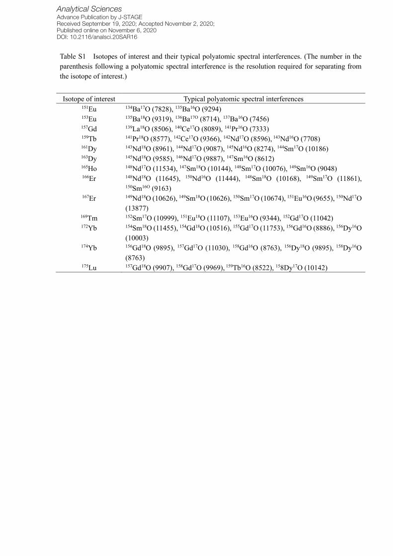
Table S1 Isotopes of interest and their typical polyatomic spectral interferences. (The number in the
parenthesis following a polyatomic spectral interference is the resolution required for separating from
the isotope of interest.)
Isotope of interest Typical polyatomic spectral interferences 151Eu 134Ba17O (7828), 135Ba16O (9294) 153Eu 135Ba18O (9319), 136Ba17O (8714), 137Ba16O (7456) 157Gd 139La18O (8506), 140Ce17O (8089), 141Pr16O (7333) 159Tb 141Pr18O (8577), 142Ce17O (9366), 142Nd17O (8596), 143Nd16O (7708) 161Dy 143Nd18O (8961), 144Nd17O (9087), 145Nd16O (8274), 144Sm17O (10186) 163Dy 145Nd18O (9585), 146Nd17O (9887), 147Sm16O (8612) 165Ho 148Nd17O (11534), 147Sm18O (10144), 148Sm17O (10076), 149Sm16O (9048) 166Er 148Nd18O (11645), 150Nd16O (11444), 148Sm18O (10168), 149Sm17O (11861),
150Sm16O (9163) 167Er 149Nd18O (10626), 149Sm18O (10626), 150Sm17O (10674), 151Eu16O (9655), 150Nd17O
(13877) 169Tm 152Sm17O (10999), 151Eu18O (11107), 153Eu16O (9344), 152Gd17O (11042) 172Yb 154Sm18O (11455), 154Gd18O (10516), 155Gd17O (11753), 156Gd16O (8886), 156Dy16O
(10003) 174Yb 156Gd18O (9895), 157Gd17O (11030), 158Gd16O (8763), 156Dy18O (9895), 158Dy16O
(8763) 175Lu 157Gd18O (9907), 158Gd17O (9969), 159Tb16O (8522), 158Dy17O (10142)
Analytical SciencesAdvance Publication by J-STAGEReceived September 19, 2020; Accepted November 2, 2020; Published online on November 6, 2020DOI: 10.2116/analsci.20SAR16

Figure Captions
Fig. 1 Shale (PAAS)-normalized REE patterns for river waters.
A: REE patterns for pristine river waters without any anthropogenic anomalies of
REEs.
B: REE patterns for German river waters with positive anthropogenic Gd anomaly.
C: REE patterns for Rhine river waters with positive anthropogenic La and Sm in
addition to Gd.
A and B were cited from Ref. 48. C was cited from. Ref.109.
Fig. 2 Structures of the main Gd compounds used as the contrast agent of MRI .
Cited from Ref. 114.
Fig. 3 Chromatogram for Gd compounds in the tap water of Berlin in Germany measured by
ZIC-cHILIC-ICP-MS. Cited from Ref. 120.
Fig. 4 Shale (PAAS)-normalized REE patterns for the shell of freshwater mussel Corbicula
fluminea. Cited from Ref. 123.
A : REE patterns for the shells collected in the Wester River, where there is no industrial
point source, and, in the Rhine River upstream of Worms, where is situated in the
industrial point source.
B : REE patterns for the shells collected in downstream of Worms.
Fig. 5 The average per capita (polulation-weighted) fluxes of 62 elements discharged by
wastewater from WWTF in Switzerlamd. The range of the element fluxes is illustrated
by the color scaling of the periodic table. Cited from Ref. 141.
Analytical SciencesAdvance Publication by J-STAGEReceived September 19, 2020; Accepted November 2, 2020; Published online on November 6, 2020DOI: 10.2116/analsci.20SAR16

Fig. 1
C
Analytical SciencesAdvance Publication by J-STAGEReceived September 19, 2020; Accepted November 2, 2020; Published online on November 6, 2020DOI: 10.2116/analsci.20SAR16

Fig. 2
Analytical SciencesAdvance Publication by J-STAGEReceived September 19, 2020; Accepted November 2, 2020; Published online on November 6, 2020DOI: 10.2116/analsci.20SAR16

Fig.3
Analytical SciencesAdvance Publication by J-STAGEReceived September 19, 2020; Accepted November 2, 2020; Published online on November 6, 2020DOI: 10.2116/analsci.20SAR16
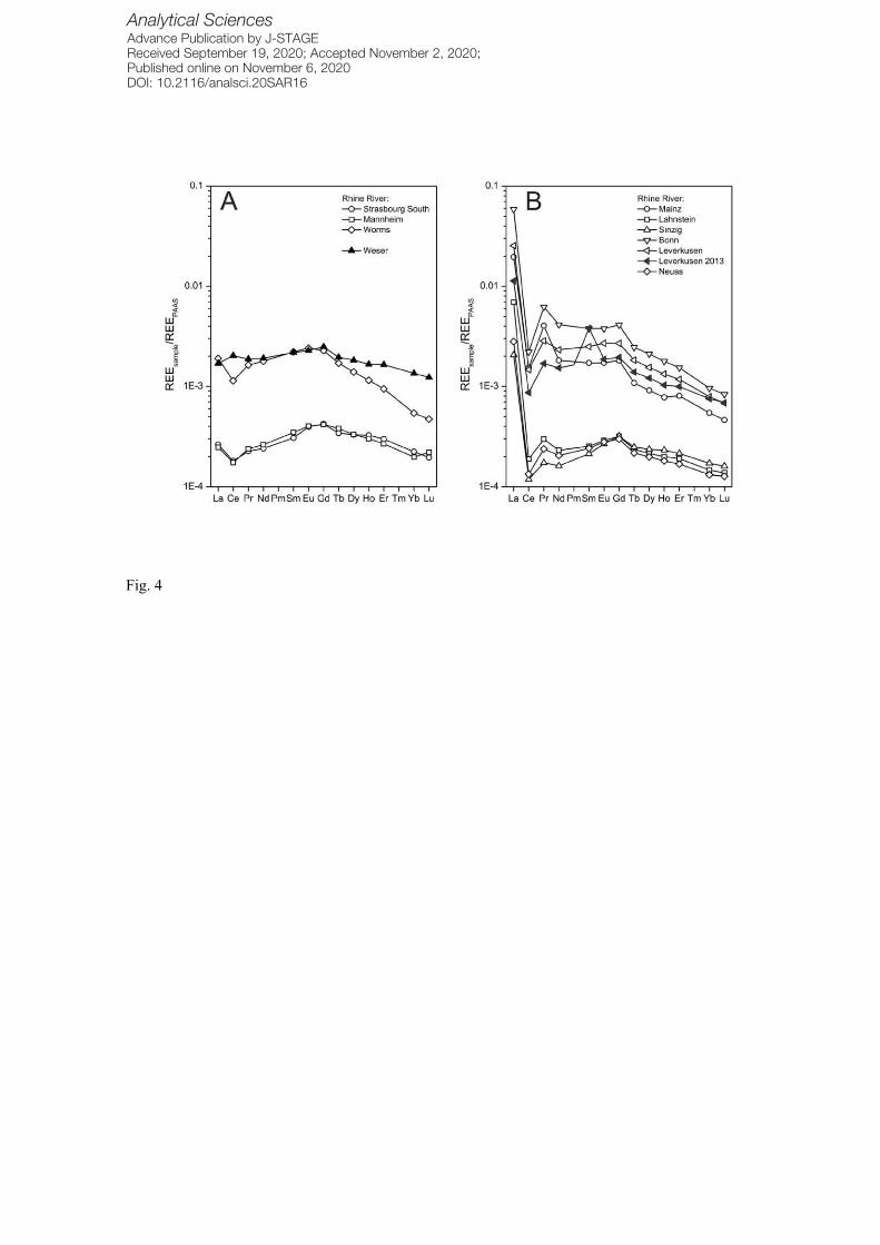
Fig. 4
Analytical SciencesAdvance Publication by J-STAGEReceived September 19, 2020; Accepted November 2, 2020; Published online on November 6, 2020DOI: 10.2116/analsci.20SAR16

Fig. 5
Analytical SciencesAdvance Publication by J-STAGEReceived September 19, 2020; Accepted November 2, 2020; Published online on November 6, 2020DOI: 10.2116/analsci.20SAR16