Postwar Slowdowns and Long-Run Growth: A Bayesian Analysis ...

Postwar Slowdowns and Long-Run Growth:

A Bayesian Analysis of Structural-Break Models

Yi-Chi Chen Eric Zivot

Department of Economics, National Cheng Kung University, Tainan, Taiwan 701, ROC

Department of Economics, University of Washington, Seattle, WA 98195, USA

corresponding author: Yi-Chi Chen, +886-6-2757575 ext. 50228

+886-6-2766491

[email protected]

Abstract Using Bayesian methods, we re-examine the empirical evidence from Ben-David,

Lumsdaine and Pappell (“Unit Roots, Postwar Slowdowns and Long-Run Growth: Evidence from Two

Structural Breaks”, Empirical Economics, 28, 2003) regarding structural breaks in the long-run growth

path of real output series for a number of OECD countries. Our Bayesian framework allows the number

and pattern of structural changes in trend and variance to be endogenously determined. We find little

evidence of postwar growth slowdowns across countries, and we find smaller output volatility for most

of the developed countries after the end of World War II. Our empirical findings are consistent with

neoclassical growth models, which predict increasing growth over the long run. The majority of the

countries we analyze have grown faster in the postwar era as opposed to the period before the first

break.

JEL classification C11, E32

Keywords Trend breaks, Growth, Gibbs sampler, Multiple structural breaks

1

1 Introduction

In this paper we re-examine the empirical findings of Ben-David, Lumsdaine and

Pappell (2003), hereafter BLP, regarding structural changes in the long-run trend of

output series using a Bayesian approach.1 They extended the one break model of

Ben-David and Papell (1995) to two structural breaks, and rejected the unit root

hypothesis in aggregate and per capita GDP for more than half of 16 OECD countries.

The two structural break model allowed them to discuss the causes of the postwar

growth slowdowns. They found that while most countries experienced postwar

slowdowns in output, they also exhibited faster growth following the second structural

break. Such increasing growth over the long run is consistent with the predictions of

Romer-type endogenous growth models. The analysis in BLP is conditional on

imposing two structural breaks and on the form of the broken trend function.2

However, they provided no formal justification for why output should only experience

exactly two breaks over the last century or why the specification of the trend functions

for certain output series should be different. In addition, they did not consider the

possibility that the variability of aggregate output may have changed over time.

Indeed, several studies (e.g. Wang and Zivot, 2000; Murray and Nelson, 2002) have

documented volatility changes in output series and have shown that changes in output

volatility can be confused with changes in trend. Our goal in this paper is to see if the

main results of BLP remain intact if we let the data determine the number and form of

the breaks in the output series.

1 See Perron (2006) for an extensive review of structural break models. 2 The criticism also applies to Ben-David and Papell (1995, 1998, 2000) in that the number of breaks is

fixed a priori.

2

We use the Bayesian methodology developed in Wang and Zivot (2000), hereafter

WZ,3 which is different in spirit than the methodology used by BLP and has several

advantages.4 First, the Bayesian approach simplifies the often complicated estimation

and inference procedures in multiple structural change models, is the same for

nonstationary and trend stationary data, and allows for exact finite-sample inferences.

Second, Bayesian inference allows for non-nested model comparisons in a

straightforward way which can be used to determine the number and form of

structural changes appropriate for a given series. Finally, the Bayesian methodology

incorporates model and parameter uncertainty explicitly.

Our empirical analysis gives comparable results to BLP’s regarding multiple breaks

in the long-run growth paths of countries. The most important distinction is the

number and form of the breaks in the output series adopted for analysis. We find

various numbers of structural breaks ranging from one to five in our Bayesian

approach, whereas BLP fixed the number of breaks at two. Furthermore, unlike in

BLP who assumed a constant variance for each output series, we find that the

majority of countries have undergone breaks in variance as well as in level and trend.

Our results agree with the findings in BLP that all of the countries have at least one

break associated with a World War or the Depression, but we provide stronger

evidence for the interruption of growth paths among the OECD countries by both

wars. Also, we do not find evidence of postwar slowdowns caused by oil price shocks

in the 1970s. Only one of the postwar breaks falls within the period of 1973-75 while

the rest occur earlier. In general, we find little evidence of postwar growth slowdowns

across countries and we find smaller output volatility for most of the developed

countries after the end of World War II. Regarding long-run growth paths, our results 3 A recent application of WZ approach to OECD unemployment rates can be seen in Summers (2004). 4 More detailed advantages of the Bayesian approach over the classical counterpart in Raftery (1994).

3

confirm the findings in BLP that most of the industrialized countries experienced

faster growth in the latter years of the sample than during the early years. These

results on sustained increasing growth are compatible with the predictions of Romer

(1986).

The remainder of our paper is organized as follows. Sections 2 and 3 review the

Bayesian methodology of WZ that we use to model multiple structural breaks in level,

trend and variance of international output series. Section 4 provides our empirical

findings on the growth path of aggregate and per capita real GDP among 16 OECD

industrialized countries and compares these results to those from BLP and other

studies. Section 5 summarizes our estimates of the long-run growth behavior of the

countries and gives a comparative analysis of the cross-country experience. Section 6

offers some concluding remarks.

2 Econometric Methodology

We assume the series of interest yt is regime-wise trend stationary and is modeled

using:5

1,

r

t t t j t j t tj

y a b t y s uφ −=

= + + +∑ (1)

| ~ (0,1) for 1,2, ,t tu iid N t TΩ = K

where tΩ denotes all available information up to time t. The model (1) allows for up

to m < T changes in level, at, trend, bt, and volatility, st. The break dates are denoted

by k1, k2,..., km such that 1 < k1 < k2 < ... < km ≤ T giving m+1 possible regimes in T

observations. Each regime i is characterized by at, bt and st which are given by the

5 Ben-David and Papell (1995) and BLP have provided strong evidence on the rejection of the unit

root null in favor of a broken trend stationary alternative for long-term output data.

4

values αi, βi and σi for i = 1, 2, ..., m+1 and ki-1 ≤ t < ki with k0 = 1 and km+1 = T+1. As

in BLP, the autoregressive parameters jφ are assumed to be identical across

regimes.6

The most general model, which we call Design I, allows for unrestricted structural

changes in level, trend and volatility such that 1 2 1, , ,t ma α α α += K ,

1 2 1, , ,t mb β β β += K and 1 2 1, , ,t ms σ σ σ += K .7 Design II only allows for structural

changes in level and trend, holding the volatility constant across regimes:8

1, 1, 2, , ,

r

t t t j t j tj

y a b t y u t Tφ σ−=

= + + + =∑ K (2)

Equations (1) and (2) can be expressed in a matrix form as:

,t t t ty x s u′= +B (3)

where 1 1i i i it k t k k t k t jx I t I y− −≤ ≤ ≤ ≤ −⎡ ⎤′ = •⎣ ⎦ , IE is an indicator variable for the event E, and

( ), ,i i iα β φ=B for i = 1, 2,..., m+1 and j = 1, 2,..., r. The vector of unknown

parameters is denoted ( ), ,′ ′ ′=θ B σ k . Given the normality assumption and the

observed data ( )1, , Ty y=Y K , the likelihood function of (3) is:

( )21

211

1( | ) exp .2

T Tt t

ttt t

y xL s

sθ

−

==

⎧ ⎫′−⎛ ⎞ ⎪ ⎪∝ −⎨ ⎬⎜ ⎟⎝ ⎠ ⎪ ⎪⎩ ⎭

∑∏B

Y (4)

6 One can adopt the Bayesian framework in Levin and Piger (2008) allowing the subset of parameters,

including the autoregressive parameters, to undergo structural breaks. 7 Other designs are also possible, such as only allowing a change in slope (kinked trend model),

restricting the trend function slope to be the same before the first break and after the second break, etc. 8 The specification is similar to ‘Model CC’ of BLP, which allows two breaks in both the intercept and

the slope of the trend function.

5

3 Bayesian Inference

In this section, we briefly describe the Bayesian framework of WZ adopted in this

study.

3.1 Prior Specification

We assume that the vectors k, B and σ2 are mutually independent and that the

elements of σ2 are independent. For the specification of the prior beliefs about

unknown parameters, we use proper priors for k, B and σ2. The break points, k, are

assumed to follow a discrete uniform distribution over all ordered subsequences of

(2,3,...,T) of length of m. This is a diffuse prior which does not impose any

information about the location of the break dates. With regard to the remaining

parameters, we employ natural conjugate priors. The prior distribution of B in

equation (3) is given by a multivariate normal (MVN) distribution,

),(~ 0 BMVN ΣBB , where B0 and ΣB are the prior mean and prior covariance matrix

of B, respectively. The prior for σ2 specifies that each element follows an independent

inverted Gamma (IG) distribution. That is, for each regime i (i = 1,..., m+1),

),(~ 002 δσ vIGi . To represent a diffuse prior, we set B0 = 0, ν0 = 1.001, δ0 = .001, and

ΣB equal to a diagonal matrix with each diagonal element equal to 1,000.

3.2 Gibbs-Sampling Algorithm

The posterior distributions of the parameters are derived using the Gibbs sampler

(Geman and Geman 1984; Gelfand and Smith 1990; Gelfand et al. 1990; Casella and

George 1992; Gelman et al. 1995; Chib and Greenberg 1996). The basic idea of the

Gibbs sampler is to approximate the joint and marginal posterior distributions by

sampling from conditional distributions. Given the full conditionals ( | , )i if θ θ− Y ,

6

where θ-i denotes the vector of θ excluding the element θi, the Gibbs-sampling

algorithm allows us to draw samples of θ iteratively from the full conditional densities.

After sufficient iteration, the draws of these random variables will converge to the

target posterior distribution ( | )f θ Y , and the marginal distribution of θi can be

approximated by the empirical distribution of the draws.

To ensure that a chain has converged, we follow the guidelines of McCulloch and

Rossi (1994), who demonstrated that the posterior distributions with trace plots can be

said to converge if the estimated densities do not vary substantially after an initial

burn-in period (so that the starting point has less influence on the chain). In our study,

these diagnostics show that convergence can be reached after a burn-in period of 500

iterations.

Before proceeding with the Gibbs sampler, we first describe the full conditionals of

the unknown parameters. WZ show that for a given break date, ki, the sample space

only depends on the neighboring break points ki-1 and ki+1. Accordingly, the posterior

conditional density of ki is of the form:

1 1( | , ) ( | , , , , )ii k i i if k f k k kθ− − +∝Y B σ Y (5)

where i = 1,..., m. The breakpoint ki can be drawn from a multinomial distribution

with a sample size parameter equal to the number of dates between ki-1 and ki+1 and

probability parameter proportional to the likelihood function. For the posterior

conditional distribution of B, the normal prior for B combined with the normal

likelihood of (4) yields a MVN conditional posterior:

( )| , ~ ,MVNθ− ΣB BB Y B %% (6)

where ( )1 20

− −′= Σ Σ +BBB B X S Y%% and ( ) 11 2 −− −′Σ = Σ +BB X S X% . Here, S is a diagonal

matrix with (s1,..., sT) along the diagonal. Finally, with the natural conjugate IG prior

7

for 2iσ and the normal likelihood (4), the posterior conditional for 2

iσ also follows

an IG distribution:

22 | , ~ ( , )

ii i iIG

σσ θ ν δ

−Y (7)

where 0 2i inν ν= + , ni represents the number of observations in regime i,

( ) ( )012

i i i iiδ δ ′= + − −Y X B Y X B , Yi is the vector of yt values and Xi is the matrix of

xt values in regime i.

Given the full conditionals (5)-(7), the Gibbs-sampling algorithm can be iterated J

times to obtain a vector sample of size J such that ( )( ) ( ) ( ) ( ), ,j j j j=θ k B σ , j = 1,..., J.9

3.3 Posterior Estimation

In order to generate the simulated draws from the Gibbs sampler, we use the method

of one long run in the MCMC algorithm suggested by Geyer (1992). Specifically,

given N = n0 + n1 iterations in the Markov chain, we only keep n1 simulated samples

for further inference by discarding the first n0 sample as a burn-in. However, the

output of the Gibbs sampler is a dependent sequence of parameter values forming a

Markov chain. As a result, the series is serially correlated but stationary and ergodic.10

Then given ),,,( )()2()1( 1niii θθθ K post-convergent sample draws, the sample mean of

these values can be used to estimate the posterior mean:

9 Details of the Gibbs sampler for the structural break models are described in WZ. The C and Gauss

codes for implementing Gibbs sampler were kindly provided by Jiahui Wang and Eric Zivot. 10 In practice there are two other remedies to produce independent sequence. The first method is to thin

the chain by taking every kth sample to reach approximate independence. However, this approach can

result in sub-optimal output (MacEachern and Berliner 1994). Another way is to batch the standard

error estimates (Ripley 1987; Geyer 1992). Although the batching provides better estimates, it is

complicated to implement in the context of time series.

8

1( )

11

1 .n

ji i

jnθ θ

=

≡ ∑ (8)

In addition, the Newey-West covariance matrix estimator that is consistent in the

presence of both heteroskedasticity and autocorrelation:

$ $0

12 1 ,

1

q

jj

jq=

⎛ ⎞Γ + − Γ⎜ ⎟+⎝ ⎠

∑ (9)

where $ jΓ is the jth-order sample autocovariance of θi from n1 simulated draws and q

is an integer of the truncation lag such that q = 4(n1 / 100)1/4, can be used to estimate

the variance of the posterior mean.

3.4 Model Selection

The Bayesian framework provides a natural way of determining the number and form

of structural breaks as a model selection problem. WZ used several model selection

criteria to determine the number and type of structural changes. Specifically, they

used marginal likelihoods, posterior odds ratios and Schwarz’s Bayes information

criterion (BIC) to select the model with the most appropriate pattern of structural

breaks that best describes the data-generating process of the series. Based on a set of

Monte Carlo experiments they found that model selection based on maximizing the

BIC performed the best,11 and so we use the BIC to select the best structural change

model for the aggregate output series.

The BIC for a model with m breaks is defined as:

ˆBIC( ) 2 ln ( | ) ln( ).m L Tλ= × −θ Y (10)

11 BIC is shown to be consistent and has good finite sample performance in selecting the number and

the type of multiple structural changes (Liu et al. 1997; Wang 2006).

9

where the likelihood function of L(⋅|⋅) is equation (4) evaluated at the posterior mean

of θ based on the output of the Gibbs sampler, λ denotes the number of estimated

parameters in model with m structural breaks, and T denotes the effective number of

observations. By the definition of (10), the model with the highest posterior

probability has the largest BIC value.12

4 Empirical Findings

The data used in this paper are based on the output series compiled by Maddison

(1991).13 The dataset contains annual GDP data for 16 industrialized countries

ranging from 1860 to 1989, and annual per capital GDP data beginning in 1870 due to

the availability of the population data.14 All the series are log transformed for the

analysis. Since output is clearly trending, two designs of structural break models

(Designs I and II) which involve breaks in the linear deterministic trend are

considered for this study.

We first present the empirical evidence for structural breaks in U.S. real GDP as an

example.15 The number of lags for the estimation of (1) and (2) is chosen based on

the BIC criterion from an ordinary least squares estimation without assuming

structural breaks. For most series, the BIC indicates one lag models.16 In order to 12 Notice that our definition of the BIC is different from that used in WZ; in other words, the BIC they

defined was the negative version of ours. Therefore, they selected the model with the smallest BIC

value. 13 The dataset was kindly provided by David Papell. 14 With availability of the country data, several countries have different beginning periods. For GDP

data, both Austria and Canada start 1870, Italy 1861, Japan 1885, Netherlands 1900, Norway 1865,

Switzerland 1899, and the United States 1869. For per capital GDP data, Japan begins 1885,

Netherlands 1900, and Switzerland 1899. 15 The detailed results of model selection and estimation for other countries are available upon request. 16 The exceptions are Netherlands real GDP and Austria per capita real GDP in which two lags are

dominant.

10

determine the number and the pattern of the structural breaks, we estimate the models

of Design I with m breaks (m = 0,1,...,4),17 and then choose the model that maximizes

the BIC criterion. Inferences are based on 2,000 draws of Gibbs sampler, after

dropping the first 500 simulations as the burn-in period. The logarithm of the

marginal likelihood and the BIC values for each model with m breaks are summarized

in Table 1. Obviously, the model with no structural breaks is not supported by the

BIC criterion. Among the competing models, the model with m = 2 breaks is favored

by the BIC. To ensure that the form of the structural breaks in variance is robust, we

also estimate the model with two breaks in level but with a constant variance over

time (Design II). For this model, the logarithm of the marginal likelihood is 197.96

and the BIC is 348.04 as shown in Table 1. Thus, the evidence is still in favor of the

model with two structural breaks in mean and variance over the model with constant

variance. Table 2 displays the results of Bayesian estimation of Design I based on the

preferred model with two structural breaks. The second column of Table 2 shows the

posterior means of the estimated parameters, followed by the unconditional means

based on the estimates in the second column using the autoregressive parameter. The

fourth and fifth columns summarize the standard deviations and medians associated

with the estimates, respectively. The last two columns report the 2.5% and 97.5%

posterior quantiles of the parameters. The last row presents the posterior mode for the

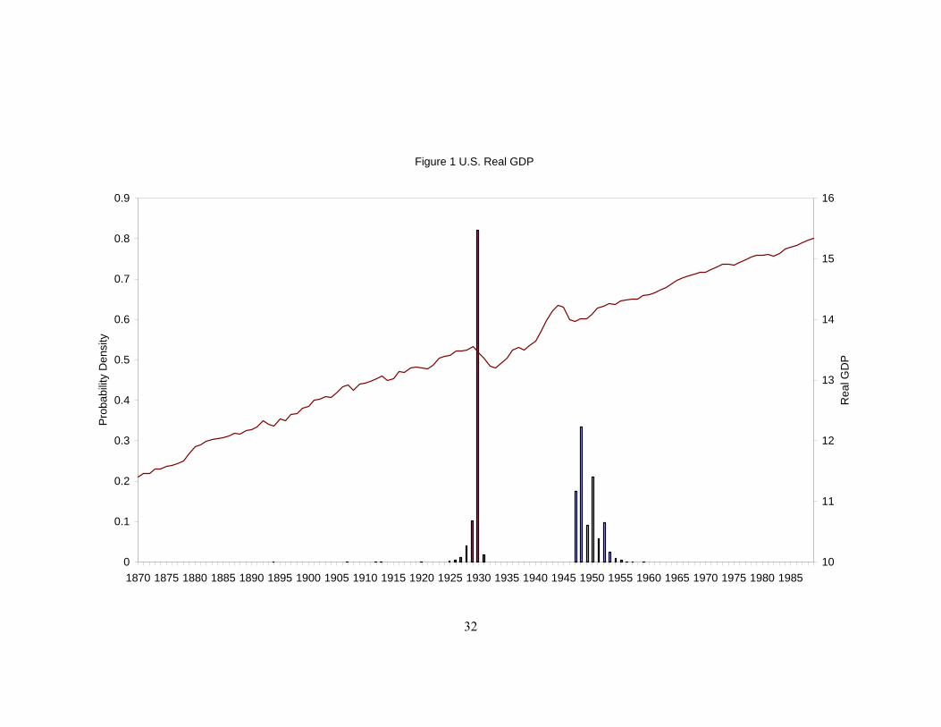
break years. Finally, Figure 1 plots the posterior distribution of the break years with

the real GDP series superimposed. As can be readily seen from the plot, the two

structural breaks most likely occurred in 1930 and in 1948 with the highest posterior

probability being around .82 and .33, respectively. The parameter estimates suggest a

takeoff in the growth rate after the break associated with the Great Depression and 17 In some occasions, the pool of candidate models has to extend to those with more than 4 breaks to

ensure the robustness of the chosen model through the model selection process.

11

that higher growth is associated with higher volatility. During the post-WWII period,

there was a significant decline in volatility of the U.S. real GDP, as the posterior mean

of σ3 was nearly one-quarter of σ2.18 These results echo those reported by Murray and

Nelson (2000, 2002) on the same data, where they showed the U.S. output swung in

1930 and then switched off in 1946, heterogeneity due to the volatile period of the

Depression followed by the fading-out phase of the post WWII was governed by a

Markov process.

With regard to the U.S. per capita real GDP, the same procedures are applied as

described above. The BIC also selects the m=2 model of Design I over the other

competing models. Again, this choice of model is warranted by comparing the model

with the same number of breaks but restricting the variance to be constant. The break

years estimated by the two-break model are similar to the case of real GDP series.

For all countries, the most preferred structural break models for real GDP and real

per capita GDP are summarized in Table 3. For the real GDP series, while Design I is

appropriate for most of countries, Design II assuming constant variance over time

better describes the dynamics of aggregate data for Finland, Japan, Sweden and

Switzerland. Similarly, for the per capita real GDP, Design I is predominant for 10

out of 16 countries, whereas Design II is appropriate for the rest. The results show

that the output series for each country underwent different structure of dynamics over

the long time horizon. In addition to breaks in level and trend, structural change in

variance is also found.

The number and the timing of structural breaks over the long-term output data vary

among the 16 countries. For real GDP, not all the aggregate data have the two-break 18 It should be noted that fixingσdoes not substantially alter the characteristics of the break model. The

segmented trends are quite similar for both designs except the second break detected by Design II

occurs three years earlier in 1945.

12

model as the preferred model. The exceptions are Australia and Canada (one break),

Austria, Belgium and Sweden (three breaks), Germany and Switzerland (four breaks),

and Japan (five breaks). Similar results are also found in the per capita series although

several countries have different numbers of structural breaks from the aggregate

data.19 These results suggest that the assumption of two breaks used by BLP is too

restrictive for some countries.

It is of interest to compare our findings on the timing of breaks with BLP, who

estimated endogenous two-break models, which only allow breaks in the intercept and

the slope of the trend function, on the same data we use.20 In their study, the wars are

the major events to cause the breaks for most of the OECD countries (especially for

all of the continental European countries).21 The United States was the only country

severely affected by the Great Depression. On the other hands, our results indicate

Canada was also plagued by the economic downturn. In fact, both North American

countries seem to share common shocks as the occurrence of their breaks were during,

or in close proximity to, the Great Depression and World War II. Furthermore, our

empirical findings provide stronger evidence for the interruption of growth paths

among the OECD countries by both wars. For example, with regard to per capita real

GDP, two-thirds of countries were affected by both World War I and II, whereas only

less than half (the Group B countries) were found in BLP.22 BLP also find a number

of post World War II breaks in the Group A countries.23 In contrast, we find little 19 In the case of the per capita output, Canada (two breaks), Germany (three breaks), Italy (five

breaks), Japan (four breaks), Netherlands (three breaks), and Sweden (two breaks). 20 The ensuing discussions mainly draw from the results of the per capita series. 21 The wars-related breaks are corroborated by the single break study of Raj (1992), Perron (1994) and

Ben-David and Papell (1995). 22 The countries of Group B are Belgium, Norway, Finland, Switzerland, and the United Kingdom. 23 The category of Group A countries in BLP includes the United States, Germany, Austria, Sweden,

Italy, Japan, Netherlands, Denmark and France.

13

evidence of postwar breaks. Only 3 out of the 16 cases did countries experience a

postwar break in the sixties and seventies.

For some countries, interesting distinctions in the timing of breaks from BLP can be

highlighted. Our results show that the only break in Australia occurred after the

Second World War, while BLP detect two breaks in 1891 and 1928 long before the

onset of the war. For Canada, our results suggest that, in addition to the Depression,

WWII also played a crucial role in the country’s growth path, but a fixed two-break

model was unable to recognize the importance of the second war. Contrary to the

view that the Crash of 1929 had exclusive impact on North America, our results

suggest that the shocks spilled over to other economies, such as Switzerland,24 where

one of the breaks over the long-term output data occurred in 1930. Also, we find

different results regarding the impact of the OPEC oil embargo during the early

1970s. BLP suggested that Denmark, France, Japan and Netherlands were severely

affected by such exogenous shocks; however, our empirical evidence does not support

such a claim. Instead, only Switzerland exhibited an oil-shock break in the mid

1970s.25 The break point was not captured by the fixed two-break model in BLP.

Finally, one of the break years in Italy’s per capita real GDP that disappeared from

BLP was associated with 1897. It represented the stage of the economic takeoff in

Italy where growth rates during the two decades prior to 1897 averaged just 0.4%

annually. During the subsequent two decades, the figure increased to nearly 4%

annually. The finding is consistent with the 4-break model of Ben-David and Papell

(2000).26

24 One of breaks in Japan’s aggregate output was associated with the Depression. 25 Japan had a oil-related break in the real GDP. 26 Nevertheless, the break that Ben-David and Papell (2000) estimated is 6 years earlier than what we

found in this study.

14

We give some explanations for the differences in results between the classical and

Bayesian methodologies. First, we do not require breaks be separated by at least five

years in the search for potential break dates and we allow for the possibility that an

outlier observation can be detected.27 Second, our model allows changes in variance

and this can affect the number and form of structural breaks.

The break points determined by our Bayesian analysis accord closely with intuition

and are more objective than the fixed two-break model used in BLP and other studies.

The posterior estimates of the preferred structural break models for aggregate and per

capita real GDP are used in the next sub-section to analyze takeoffs and slowdowns.

5 Growth Implications

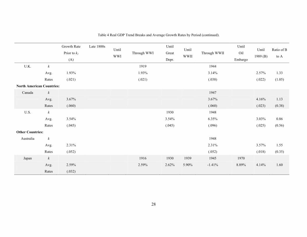
Based on the empirical evidence of the structural breaks, the growth implications of

the OECD countries can be analyzed to address some common features in terms of the

timing of the breaks, regional characteristics and severity of the slowdowns.

From the estimated break dates across 16 countries, the past 130 years (120 years in

the case of per capita real GDP) can distinguish eight distinct regimes by the major

events in history (Tables 4 and 5).28 Each country experienced a subset period of

these regimes as the first period begins in 1860 for the aggregate data (1870 for the

per capita data) and ends in 1989.29 The timing and the frequency of the breaks can

be used to delineate the 16 industrialized countries into three regional groups, with the

twelve countries in continental Europe in one group, two countries in North America

and the two remaining countries in the other.

27 A potential outlier is identified by two break dates next to each other. 28 Ben-David and Papell (2000) used the similar partition over the period. 29 Some countries begin with a different year depending on the data availability. See footnote 8.

15

The columns of Tables 4 (the aggregate data) and 5 (the per capita data) summarize

the characteristics across the various regimes. The break years for each country are

shown in the first row for the specific country. The numbers below the break year are

the estimated average annual growth rates and the estimated volatilities for the period

(in parentheses).

Figures 2 and 3 outline the relationship between the time spans of each period for

each of the countries and the average growth and the volatility exhibited by each

country during the time spans. For per capita real GDP among the 16 countries, only

Italy, Switzerland and Japan exhibited a significant postwar break, and their

slowdowns began in close proximity to the OPEC oil embargo.30 For example, Japan

had an average annual growth rate of more than 7% prior to 1970 and then dropped to

3% after the break. In that sense, we confirm the finding in BLP that the oil shock was

not the leading cause of the postwar slowdowns from the long-run perspective.31 As

is addressed in Ben-David and Papell (2000), the collapse of the Bretton Woods

system during the early 1970s, along with the concurrent oil price shocks, might

jointly contribute to postwar slowdowns. It is also worthwhile to note that the

slowdowns in the growth rate do not affect the volatility across the regimes. In fact,

for those countries that experienced postwar slowdowns, the volatility in their output

tends to remain constant over the long-term time spans.

The evidence on the growth slowdown in our study is consistent with the findings in

Ben-David and Papell (2000) for the G7 countries, where only two cases of postwar

growth slowdowns were observed. In addition, our analysis extends beyond the G7

countries and shows that most OECD countries do not exhibit a significant postwar

30 For the aggregate cases, the postwar breaks were present in Sweden, Switzerland and Japan. 31 However, the countries and the timing of postwar beaks in our analysis are different from BLP (One

exception is Japan, still the timing is different).

16

break in their growth rates, and finds higher postwar growth for most of the countries

than its initial rate prior to the first break. The last column in Table 5 indicates the

extent of the postwar slowdowns from the long-run perspective. 32 After the

post-WWII slowdown, all of these countries experienced higher average growth rates

than they had exhibited prior to their first breaks. In the case of Italy, average final

period growth rate was 711 percent of first period rate. Also, final period growth rate

in Switzerland was 142 percent of first period rate, and 222 percent higher than

prebreak rate in Japan. In general, postwar growth for each of the OECD countries is

considerably higher than the growth rate prior to the first break.

In terms of volatility across regimes, we find strong evidence of a more stabilized

economy during the postwar era. Contrary to the common perception that the U.S.

economy stabilized in the early 1980’s (see McConnell and Perez-Quiros 2000;

Warnock and Warnock 2000; and Kim et al. 2004), when the postwar volatility

reduction issue is examined from the long-run perspective of 120 years of the

aggregate data rather than just postwar data alone, there is evidence of a significant

reduction in postwar volatility.33 Our results show that the volatility reduction in

output started as early as the end of WWII. From Figures 2 and 3, except for three

continental European countries, postwar volatility for the rest of the 13 countries has

fallen considerably, or at least remained steady, as opposed to its multidecade initial

period.

Focusing on per capita output levels and growth rates, the Second World War had a

worldwide impact on the major industrialized countries. Each of the countries (other

than Finland and Sweden) experienced a significant structural change after the end of

32 Less evidence of postwar slowdowns was observed in the aggregate series (Table 6). 33 The studies referred in this paragraph only limit to the U.S. case. In addition, these studies based on

postwar data cannot reflect the magnitude of the volatility reduction from a long-run perspective.

17

the war. 34 The new postwar per capita growth rates of these countries were

considerably higher than the baseline rates of growth. In the meantime, there is a

significant volatility reduction during the postwar era compared to the baseline levels

of volatility. While World War I severely affected the continental European countries

(and Japan), the Great Depression resulted in a significant structural break in only two

North American countries and Switzerland. The Great Depression regime for both the

United States and Canada was characterized by level drops but trend increases during

the following period. In the case of the United States, the drop in level following the

1930 break came along with the average annual growth rate of 6.4% between 1931

and 1947. In the case of Canada, the drop in level boosted the economy to a higher

growth rate that averaged 11.6% between 1932 through 1945. Furthermore, the two

economies had a distinct reaction to the Great Depression shock. While Canada

experienced a lower volatility after the shock, the economic downturn has brought

about twice as much as the pre-break level of the variance in the U.S. economy.

6 Conclusions

Using Bayesian methods we search for the most appropriate structural break

specification to model the changes in the growth processes of 16 OECD countries

using up to 130 years of annual aggregate and per capita GDP data. Our analysis

focuses on three aspects of the structure change models. First, we characterize

distinct regimes based on changes in the level, the trend and the variance. Second, we

conduct a comparative study of the cross-country experience to establish stylized

facts of growth rates. Finally, we make comparisons of empirical findings between

34 Ben-David and Papell (2000) find that the three continental European countries (France, Germany

and Italy) experienced trend breaks before and after World War II.

18

previously published results using classical procedures and our results based on a

Bayesian procedure in order to present different views on long-run growth paths

under alternative methodologies.

Using long spans of data, we find that the countries under study underwent between

two and five different periods of development in which the major events such as the

wars and the Great Depression have played a crucial role in explaining the breaks in

the growth path. Depending on the patterns of the dynamics in the series, each regime

can differ in level, growth rate, variance, and all three types of changes are observed

in the majority of cases. The results from the model selection in our study suggest

that the two-break models in BLP impose undue restrictions on the underlying

structure of dynamics in the long-term output series. Without any prior assumptions

on the number of structural breaks, our Bayesian approach sheds different light on the

progress of output across the major industrialized countries.

Our empirical evidence on postwar growth slowdowns further supports the findings

of Ben-David and Papell (2000) in which no strong indication of the slowdowns

occurred across countries. Furthermore, we document some stylized facts regarding

the volatility reduction in the aggregate and per capita real GDP. The trend towards

less volatile economies for most of the developed countries is observed after the end

of World War II, when examined from the long-run perspective of more than 120

years. By comparing the postwar growth rate with the baseline rate, we find that

growth rates increased over extended periods of time. In this sense, the evidence of

the high postwar growth reflected the high transitional high growth and is compatible

with the prediction of the endogenous growth models.

19

Acknowledgments

The first author gratefully acknowledges financial support from the National Science Council in

Taiwan, under Contract NSC 93-2415-H-006-003. The second author gratefully acknowledges

financial support from the Gary Waterman Distinguished Scholar Fund.

20

References

Ben-David D, Pappell DH (1995) The great wars, the great crash, and steady state growth: some new

evidence about an old stylized fact. J Monet Econ 36:453–475

Ben-David D, Pappell DH (1998) Slowdowns and meltdowns: postwar growth evidence from 74

countries. Rev Econ Stat 80:561–571

Ben-David D, Pappell DH (2000) Some evidence on the continuity of the growth process among the

G7 countries. Econ Inq 38:320–330

Ben-David D, Lumsdaine RL, Papell DH (2003) Unit roots, postwar slowdowns and long-run growth:

evidence from two structural breaks. Empir Econ 28:303–319

Casella G, George EI (1992) Explaining the Gibbs sampler. Am Stat 46:167–174

Cheung YW, Chinn MD (1996) Deterministic, stochastic, and segmented trends in aggregate output: a

cross-country analysis. Oxf Econ Pap 48:134–162

Chib S, Greenberg E (1996) Markov Chain Monte Carlo simulation methods in econometrics. Econ

Theory 12:409–431

Gelfand AE, Smith AFM (1990) Sampling-based approaches to calculating marginal densities. J Am

Stat Assoc 85:398–409

Gelfand AE, Hills SE, Racine-Poon A, Smith AFM (1990) Illustration of Bayesian inference in normal

data models using Gibbs sampling. J Am Stat Assoc 85:972–985

Gelman A, Carlin JS, Stern HS, Rubin DB (1995) Bayesian data analysis. Chapman and Hall, London

Geman S, Geman D (1984) Stochastic relaxation, Gibbs distributions and the Bayesian restoration of

images,” IEEE Trans on Pattern Anal Mach Intell 6:721–741

Geyer CJ (1992) Practical Markov Chain Monte Carlo. Stat Sci, 7:473–483

Kim C-J, Nelson C, Piger J (2004) The less volatile U.S. economy: a Bayesian investigation of timing,

breadth, and potential explanations. J Bus Econ Stat 22:80–93

21

Levin AT, Piger JM (2008) Bayesian model selection of structural break models. Available at SSRN:

http://ssrn.com/abstract=1132463

Liu J, Wu S, Zidek JV (1997) On segmented multivariate regressions. Stat Sin 7: 497-525.

MacEachern SN, Berliner LM (1994) Subsampling the Gibbs sampler. Am Stat 48:188–190

Maddison A (1991) Dynamic forces in capitalist development: a long-run comparative view. Oxford

University Press, Oxford

Murray C, Nelson CR (2000) The uncertain trend in US GDP. J Monet Econ 46:79-95

Murray C, Nelson CR (2002) The great depression and output persistence. J Money Credit Bank

34:1090-1098

McConnell MM, Perez-Quiros G (2000) Output fluctuations in the United States: what has changed

since the early 1980’s? Am Econ Rev 90:1464–1476

McCulloch R, Rossi PE (1994) An exact likelihood analysis of the multinomial probit model. J Econ

64: 207–240

Perron P (1994) Trend, unit root and structural change in macroeconomic time series. In: Rao BB (ed)

Cointegration for the applied economist. Macmillan Press, Basingstoke, pp 113–146

Perron P (2006) Dealing with structural breaks. In: Patterson K, Mills TC (eds) Palgrave Handbook of

Econometrics, vol. 1, Palgrave Macmillan, New York, pp 278–352

Raftery AE (1994) Changepoint and change curve modeling in stochastic processes and spatial

statistics. J Appl Stat Sci 1:403–424

Raj B (1992) International evidence on persistence in output in the presence of an episodic change. J

Appl Econ 7:281–293

Ripley BD (1987) Stochastic Simulation. Wiley, New York

Romer PM (1986) Increasing returns and long run growth. J Political Econ 94:1002–1038

Summer PM (2004) Bayesian evidence on the structure of unemployment. Econ Letters 83: 299-306.

Wang J, Zivot E (2000) A Bayesian time series model of multiple structural changes in level, trend,

and variance. J Bus Econ Stat 18:374–386

22

Wang, Z (2006). The joint determination of the number and the type of structural changes. Econ

Letters, 93:222-227

Warnock MV, Warnock FE (2000) The declining volatility of U.S. employment: was Arthur Burns

right? Board of Governors of the Federal Reserve System International Finance Discussion Papers.

23

Table 1 Model Selection for US Real GDPa

Design I

mb m=0 m=1 m=2 m=3 m=4

LLKc 176.192 174.530 206.056 212.628 209.653

BICd 333.235 310.760 354.663 348.656 323.557

Design II

LLK 173.760 197.959 201.188 189.799

BIC 314.008 348.044 340.137 302.998

Note:

a. This table summarizes the results of the choice of model based on the Schwarz’s Bayesian

Information Criterion (BIC). The specifications for each candidate design are given by

equations (1) and (2), respectively.

b. The number of breaks in the model.

c. The marginal log-likelihood value.

d. The Schwarz’s BIC is calculated by 2*LLK- λ*log(T) where LLK is the marginal likelihood

value evaluated at the posterior mean of the parameter, λ is the number of parameters with m

structural breaks and T is the number of observations.

24

Table 2 Parameter Estimates for U.S. Real GDP

(1860~1989, annually)

parameter mean implied meanstd.

deviation median

posterior quantiles

2.5% 97.5%

α1 3.271 11.541 .669 3.260 1.951 4.667

α2 2.638 9.309 .710 2.648 1.319 4.035

α3 3.337 11.774 .684 3.334 2.020 4.732

β1 .010 .035 .002 .010 .006 .014

β2 .018 .063 .007 .018 .008 .030

β3 .009 .030 .002 .009 .005 .012

φ1 .717 .059 .718 .593 .832

σ1 .045 .005 .044 .037 .054

σ2 .096 .019 .094 .070 .134

σ3 .025 .004 .025 .020 .032

k1 =1930 k2 =1948

Note: the parameter estimates are corresponding to those in equation (1) and k indicates the break

years.

25

Table 3 Summary of Break Years

Real GDP

Country Design k1 k2 k3 k4 k5

Australia I 1948

Austria I 1914 1945 1946

Belgium I 1914 1919 1944

Canada I 1947

Denmark I 1915 1947

Finland II 1917 1919

France I 1917 1947

Germany I 1862 1914 1945 1947

Italy I 1943 1948

Japan II 1916 1930 1939 1945 1970

Netherlands I 1944 1947

Norway I 1912 1945

Sweden II 1917 1918 1964

Switzerland II 1917 1930 1945 1975

U.K. I 1919 1944

U.S. I 1930 1948

Per Capita Real GDP

Country Design k1 k2 k3 k4 k5

Australia I 1947

Austria I 1914 1945 1946

Belgium I 1914 1919 1944

Canada I 1931 1945

Denmark I 1915 1947

Finland II 1917 1919

France I 1917 1947

Germany I 1914 1945 1948

Italy II 1897 1919 1943 1946 1968

Japan II 1916 1939 1945 1969

Netherlands II 1919 1944 1947

Norway I 1917 1949

Sweden II 1917 1918

Switzerland II 1917 1930 1945 1975

U.K. I 1919 1944

U.S. I 1930 1947

26

Table 4 Real GDP Trend Breaks and Average Growth Rates by Period

Growth Rate

Prior to k1

(A)

Late 1800s Until

WWI Through WWI

Until

Great

Depr.

Until

WWII Through WWII

Until

Oil

Embargo

Until

1989 (B)

Ratio of B

to A

Continental European Countries:

Austria k 1914 1945, 1946

Avg.

Rates

2.49%

(.022)

2.49%

(.022)

2.82%, 4.38%

(.067), (.056)

3.26%

(.031)

1.31

(1.41)

Belgium k 1914, 1919 1944

Avg.

Rates

1.99%

(.013)

1.99%, -37.75%

(.013), (.091)

-3.75%

(.044)

3.05%

(.021)

1.53

(1.62)

Denmark k 1915 1947

Avg.

Rates

2.90%

(.020)

2.90%

(.020)

2.48%

(.062)

2.14%

(.025)

0.74

(1.25)

Finland k 1917, 1919

Avg.

Rates

2.62%

(.036)

2.62%, -8.00%

(.036)

3.78%

1.44

France k 1917 1947

Avg.

Rates

1.22%

(.051)

1.22%

(.051)

71.15%

(.120)

2.39%

(.019)

1.96

(0.37)

27

Growth Rate

Prior to k1

(A)

Late 1800s Until

WWI

Through WWI Until

Great

Depr.

Until

WWII Through WWII

Until

Oil

Embargo

Until

1989 (B)

Ratio of B

to A

Germany k 1862 1914 1945, 1947

Avg.

Rates

369.40%

(.060)

369.40%

(.060)

2.72%

(.023)

5.26%, -194.07%

(.073), (.053)

2.41%

(.020)

0.01

(0.33)

Italy k 1943, 1948

Avg.

Rates

2.04%

(.047)

2.04%, 119.18%

(.047), (.159)

2.85%

(.022)

1.40

(0.47)

Netherlands k 1944, 1947

Avg.

Rates

-0.04%

(.055)

-0.04%, 994.82%

(.055), (.039)

1.90%

(.024)

49.50

(0.44)

Norway TB 1912 1945

Avg.

Rates

1.81%

(.019)

1.81%

(.019)

2.51%

(.056)

3.96%

(.018)

2.19

(0.95)

Sweden k 1917, 1918 1964

Avg.

Rates

2.10%

(.027)

2.10%, 9.01%

(.027)

3.22%

2.20%

1.05

Switzerland k 1917 1930 1945 1975

Avg.

Rates

2.18%

(.023)

2.18%

(.023)

5.14%

0.80%

4.28%

2.07%

0.95

Table 4 Real GDP Trend Breaks and Average Growth Rates by Period (continued).

28

Growth Rate

Prior to k1

(A)

Late 1800s Until

WWI Through WWI

Until

Great

Depr.

Until

WWII Through WWII

Until

Oil

Embargo

Until

1989 (B)

Ratio of B

to A

U.K. k 1919 1944

Avg.

Rates

1.93%

(.021)

1.93%

(.021)

3.14%

(.038)

2.57%

(.022)

1.33

(1.05)

North American Countries:

Canada k 1947

Avg.

Rates

3.67%

(.060)

3.67%

(.060)

4.16%

(.023)

1.13

(0.38)

U.S. k 1930 1948

Avg.

Rates

3.54%

(.045)

3.54%

(.045)

6.35%

(.096)

3.03%

(.025)

0.86

(0.56)

Other Countries:

Australia k 1948

Avg.

Rates

2.31%

(.052)

2.31%

(.052)

3.57%

(.018)

1.55

(0.35)

Japan k 1916 1930 1939 1945 1970

Avg.

Rates

2.59%

(.032)

2.59%

2.62%

5.90%

-1.41%

8.89%

4.14%

1.60

Table 4 Real GDP Trend Breaks and Average Growth Rates by Period (continued).

29

Table 5 Per Capita Real GDP Trend Breaks and Average Growth Rates by Period

Growth Rate

Prior to k1 (A)

Late

1800s

Until

WWI Through WWI

Until Great

Depr.

Until

WWII Through WWII

Until

Oil Embargo

Until

1989

(B)

Ratio of B

to A

Continental European Countries:

Austria k 1914 1945, 1946

Avg. Rates 1.60%

(.021)

1.60%

(.021)

2.27%, 22.94%

(.063), (.076)

3.28%

(.030)

2.05

(1.43)

Belgium k 1914, 1919 1944

Avg. Rates 0.99%

(.014)

0.99%, -24.47%

(.014), (.089)

-2.52%

(.042)

2.90%

(.021)

2.93

(1.50)

Denmark k 1915 1947

Avg. Rates 1.88%

(.018)

1.88%

(.018)

1.43%

(.062)

2.33%

(.024)

1.24

(1.33)

Finland k 1917, 1919

Avg. Rates 1.45%

(.035)

1.45%, 12.23%

(.035)

3.10%

2.14

(1.00)

France k 1917 1947

Avg. Rates 0.95%

(.041)

0.95%

(.041)

2.32%

(.120)

2.30%

(.018)

2.42

(0.44)

30

Growth Rate

Prior to k1 (A)

Late

1800s

Until

WWI Through WWI

Until Great

Depr.

Until

WWII Through WWII

Until

Oil Embargo

Until

1989 (B)

Ratio of B

to A

Germany k 1914 1945, 1948

Avg. Rates 1.64%

(.022)

1.64%

(.022)

4.41%, 170.56%

(.069), (.420)

2.37%

(.019)

1.45

(0.86)

Italy k 1897 1919 1943, 1946 1968

Avg. Rates 0.37%

(.029)

0.37%

(.029)

3.51%

1.36%, -27.33%

5.14%

2.63%

7.11

(1.00)

Netherlands k 1919 1944, 1947

Avg. Rates -1.22%

(.036)

-1.22%

(.036)

-3.12%, 323.40%

2.06%

3.33

(1.00)

Norway k 1917 1949

Avg. Rates 1.09%

(.019)

1.09%

(.019)

2.13%

(.058)

3.40%

(.018)

3.12

(0.95)

Sweden k 1917, 1918

Avg. Rates 1.33%

(.027)

1.33%, 29.82%

(.027)

2.84%

2.14

(1.00)

Switzerland k 1917 1930 1945 1975

Avg. Rates 1.11%

(.021)

1.11%

(.021)

4.80%

0.31%

2.87%

1.58%

1.42

(1.00)

Table 5 Per Capita Real GDP Trend Breaks and Average Growth Rates by Period (continued).

31

Growth Rate

Prior to k1 (A)

Late

1800s

Until

WWI Through WWI

Until Great

Depr.

Until

WWII Through WWII

Until

Oil Embargo

Until

1989 (B)

Ratio of B

to A

U.K. k 1919 1944

Avg. Rates 1.07%

(.021)

1.07%

(.021)

2.18%

(.037)

2.15%

(.018)

2.01

(0.86)

North American Countries:

Canada k 1931 1945

Avg. Rates 2.08%

(.053)

2.08%

(.053)

11.62%

(.049)

2.84%

(.024)

1.37

(0.45)

U.S. k 1930 1947

Avg. Rates 1.69%

(.044)

1.69%

(.044)

6.38%

(.090)

1.90%

(.027)

1.12

(0.61)

Other Countries:

Australia k 1947

Avg. Rates 0.55%

(.053)

0.55%

(.053)

2.20%

(.017)

4.00

(0.32)

Japan k 1916 1939 1945 1969

Avg. Rates 1.49%

(.037)

1.49%

(.037)

1.44%

-1.15%

7.69%

3.31%

2.22

(1.00)

Table 5 Per Capita Real GDP Trend Breaks and Average Growth Rates by Period (continued).

32

Figure 1 U.S. Real GDP

0

0.1

0.2

0.3

0.4

0.5

0.6

0.7

0.8

0.9

1870 1875 1880 1885 1890 1895 1900 1905 1910 1915 1920 1925 1930 1935 1940 1945 1950 1955 1960 1965 1970 1975 1980 1985

Prob

abilit

y D

ensi

ty

10

11

12

13

14

15

16

Rea

l GD

P

33

Figure 2 Average Annual Real GDP Growth Rates Each Period

Continental European Countries

1860 1870 1880 1890 1900 1910 1920 1930 1940 1950 1960 1970 1980 1990

YEAR

Austria

Belgium

Finland

Denmark

France

Germany

Italy

Netherlands

Norway

Sweden

Switzerland

U.K.

2.49%(.022) 2.82%(.067) 3.26%(.031)

1.99%(.013) -37.75%(.091) 3.05%(.021)

2.90%(.020) 2.48%(.062) 2.14%(.025)

2.62%(.036) -8.00% 3.78%

1.22%(.051) 71.15%(.120) 2.39%(.019)

369.40%(.060) 2.72%(.023) 5.26%(.073) -194.07%(.053) 2.41%(.020)

-0.04%(.055)

119.18%(.159) 2.85%(.022)

994.82%(.039) 1.90%(.024)

1.81%(.019) 2.51%(.056) 3.96%(.018)

2.10%(.027) 3.22% 2.20%

2.18%(.023) 5.14% 0.80% 4.28% 2.07%

1.93%(.021) 3.14%(.038) 2.57%(.022)

2.04%(.047)

-3.75%(.044)

Note: the horizontal line indicates time span of period with average growth. Volatility is in parentheses and for those without

breaks in variance volatility is specified in the first period only. Outliers identified are not appeared on the time line.

34

Figure 2 Average Annual Real GDP Growth Rates Each Period (continued)

Other Countries

1860 1870 1880 1890 1900 1910 1920 1930 1940 1950 1960 1970 1980 1990

Year

Canada

U.S.

Australia

Japan

3.67%(.060) 4.16%(.023)

3.54%(.045) 6.35%(.096) 3.03%(.025)

2.31%(.052) 3.57%(.018)

2.59%(.032) 2.62% 5.90% -1.41% 8.89% 4.14%

North American Countries



35

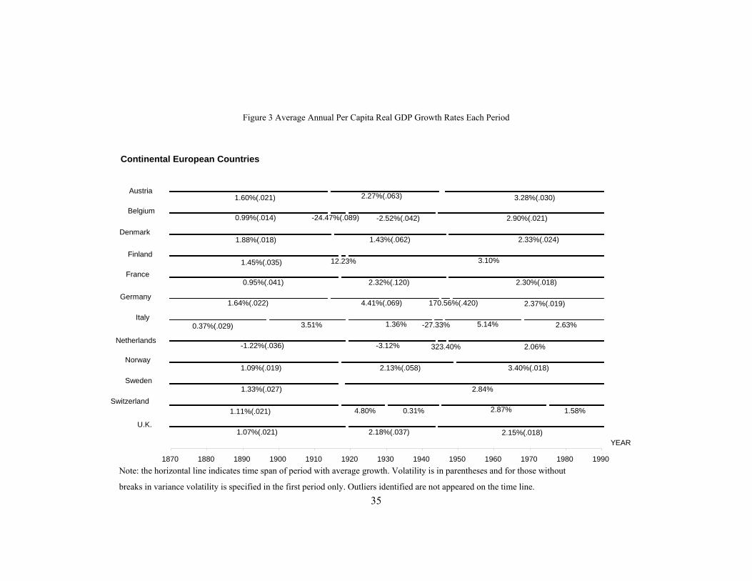
Figure 3 Average Annual Per Capita Real GDP Growth Rates Each Period

Continental European Countries

1870 1880 1890 1900 1910 1920 1930 1940 1950 1960 1970 1980 1990

YEAR

Belgium

Denmark

Finland

France

Germany

Italy

Netherlands

Norway

Sweden

Switzerland

U.K.

Austria1.60%(.021) 2.27%(.063) 3.28%(.030)

0.99%(.014) -24.47%(.089) -2.52%(.042) 2.90%(.021)

1.88%(.018) 1.43%(.062) 2.33%(.024)

1.45%(.035) 12.23% 3.10%

0.95%(.041) 2.32%(.120) 2.30%(.018)

1.64%(.022) 4.41%(.069) 170.56%(.420) 2.37%(.019)

0.37%(.029) 3.51% 1.36% -27.33% 5.14% 2.63%

-1.22%(.036) -3.12% 323.40% 2.06%

1.09%(.019) 2.13%(.058) 3.40%(.018)

1.33%(.027) 2.84%

1.11%(.021) 4.80% 0.31% 2.87% 1.58%

1.07%(.021) 2.18%(.037) 2.15%(.018)



36

Figure 3 Average Annual Per Capita Real GDP Growth Rates Each Period (continued)

Other Countries

1870 1880 1890 1900 1910 1920 1930 1940 1950 1960 1970 1980 1990

Year

Canada

U.S.

Australia

Japan

2.08%(.053) 11.62%(.049) 2.84%(.024)

1.69%(.044) 6.38%(.090) 1.90%(.027)

0.55%(.053) 2.20%(.017)

1.49%(.037) 1.44% -1.15% 7.69% 3.31%

North American Countries



Postwar Slowdowns and Long-Run Growth: A Bayesian Analysis ...

Documents

Transcript of Postwar Slowdowns and Long-Run Growth: A Bayesian Analysis ...