http://www.diva-portal.org

Postprint

This is the accepted version of a paper presented at GPC 2017 : The 12th InternationalConference on Green, Pervasive and Cloud Computing, Cetara, Amalfi Coast, Italy.

Citation for the original published paper:

García Martín, E., Lavesson, N., Grahn, H. (2017)Identification of Energy Hotspots: A Case Study of the Very Fast Decision Tree.In: Au M., Castiglione A., Choo KK., Palmieri F., Li KC. (ed.), GPC 2017: Green,Pervasive, and Cloud Computing (pp. 267-281). Cham, Switzerland: SpringerLecture Notes in Computer Sciencehttps://doi.org/10.1007/978-3-319-57186-7_21

N.B. When citing this work, cite the original published paper.

Permanent link to this version:http://urn.kb.se/resolve?urn=urn:nbn:se:bth-15490

Identification of Energy Hotspots:A Case Study of the Very Fast Decision Tree

Eva Garcia-Martin�, Niklas Lavesson, and H̊akan Grahn

Blekinge Institute of Technology, Karlskrona, Sweden.eva.garcia.martin@bth.se

Abstract. Large-scale data centers account for a significant share ofthe energy consumption in many countries. Machine learning technol-ogy requires intensive workloads and thus drives requirements for lots ofpower and cooling capacity in data centers. It is time to explore greenmachine learning. The aim of this paper is to profile a machine learningalgorithm with respect to its energy consumption and to determine thecauses behind this consumption. The first scalable machine learning al-gorithm able to handle large volumes of streaming data is the Very FastDecision Tree (VFDT), which outputs competitive results in comparisonto algorithms that analyze data from static datasets. Our objectives areto: (i) establish a methodology that profiles the energy consumption ofdecision trees at the function level, (ii) apply this methodology in an ex-periment to obtain the energy consumption of the VFDT, (iii) conducta fine-grained analysis of the functions that consume most of the energy,providing an understanding of that consumption, (iv) analyze how differ-ent parameter settings can significantly reduce the energy consumption.The results show that by addressing the most energy intensive part ofthe VFDT, the energy consumption can be reduced up to a 74.3%.

Keywords: machine learning · big data · Very Fast Decision Tree · greenmachine learning · data mining · data stream mining

1 Introduction

Current advancements in hardware together with the availability of large vol-umes of data, have inspired the field of machine learning into developing state-of-the-art algorithms that can process these volumes of data in real-time. For thatreason, many machine learning algorithms are being implemented in big dataplatforms and in the cloud [22]. Examples of such applications are Apache Ma-hout and Apache SAMOA [4], frameworks for distributed and scalable machinelearning algorithms.

There are several desired properties for an algorithm to handle large vol-umes of data: processing streams of data, adaptation to the stream speed, anddeployment in the cloud. The Very Fast Decision Tree (VFDT) algorithm [6] isthe first machine learning algorithm that is able to handle potentially infinitestreams of data, while obtaining competitive predictive performance results in

II

comparison to algorithms that analyze static datasets. Since these algorithms of-ten run in the cloud, an energy efficient approach to the algorithm design couldsignificantly affect the overall energy consumption of the cluster of servers.

The VFDT and other streaming algorithms are only evaluated in terms ofscalability and predictive performance. The aim of this paper is to profile theVery Fast Decision Tree algorithm with respect to its energy consumption andto determine the causes behind this consumption. Our objectives are to: (i) es-tablish a methodology that profiles the energy consumption of decision treesat the function level, (ii) apply this methodology in an experiment with fourlarge datasets (10M examples) to obtain the energy consumption of the VFDT,(iii) conduct a fine-grained analysis of the functions that consume most of theenergy, providing an understanding of that consumption, (iv) analyze how dif-ferent parameter settings can significantly reduce the energy consumption. Wehave identified the part of the algorithm that consumes the most amount of en-ergy, i.e. the energy hotspot. The results suggest that the energy can be reducedup to a 74.3% by addressing the energy hotspot and by parameter tuning thealgorithm.

The paper is organized as follows. In Section 2 we give a background expla-nation of decision trees and the VFDT, continuing with a review of related work.In Section 3 we explain the proposed method to profile energy consumption andhow to apply it to the VFDT. Sections 4 and 5 present the experiment and theresults and analysis of the experiment. Finally, we present the conclusions andpointers to future work in Section 6.

2 Background

2.1 Decision Trees and Very Fast Decision Tree (VFDT)

In a classification problem, we have a set of examples in the form (x, y). x repre-sents the features or attributes, and y represents the label to be predicted. Thegoal is to find the function, or model, that predicts y given x (y = f(x)) [6].Decision trees are a common type of algorithms used in machine learning thatrepresent f in the form of a tree. A node in the tree represents a test on an at-tribute, and the branches of such node, known as literals, represent the attributevalues. The leaves represent the labels y. When the model is built, in order topredict the label of a new example xi, the example passes through the nodesbased on the different attribute values, until it reaches a leaf. That leaf will bethe label y. In order to build the model, the algorithm uses a divide-and-conquerapproach. The dataset is passed to the first node, and based on that data chunk,the attribute with the highest information gain is chosen as the root node. Thedataset is then split based on that attribute choice, and each chunk of data ispassed to the corresponding child. The process is repeated recursively on eachnode, until the information is homogeneous enough, then the leaf is labeledwith the appropriate class.

Very Fast Decision Tree (VFDT) [6] is a decision tree algorithm that buildsa tree incrementally. The data is analyzed sequentially and only once. The al-

III

gorithm analyzes the first n instances of the data stream, and chooses the bestattribute as the root node. This node is updated with the literals, each beinga leaf. The following examples will be passed to the next leaves and follow thesame procedure of replacing leaves by decision nodes. On each iteration, thestatistics on each leaf are updated with the new example values. This is doneby first sorting an example to a leaf l, based on the attribute values of thatexample and on the parent nodes, and then updating the times each attributevalue is observed in l. After a minimum number of examples n are seen in l,the algorithm calculates the two attributes with the highest information gain(G). Let ∆G = G(Xa) −G(Xb) be the difference between the information gainof both attributes. If ∆G > ε the leaf is substituted by an internal node withthe attribute with highest G. ε represents the Hoeffding Bound [10], shown inEq.1. This bound states that the chosen attribute at a specific node after seeingn number of examples, will be the same attribute as if the algorithm had seeninfinite number of examples, with probability 1-δ.

ε =

√R2 ln(1/δ)

2n(1)

2.2 Related Work

This section focuses on two areas. The first area regarding energy efficiencyin computing and the second relating machine learning, big data and energyefficiency.

Many energy-aware hardware solutions have been implemented. For instance,the Dynamic Voltage Frequency Scaling (DVFS) power saving technique is usedin many contemporary processors. Several energy-saving approaches present en-ergy efficient solutions for computation [21]. Regarding green computing at thesoftware level, several publications [19, 11, 8] address the importance of develop-ing energy-aware solutions, applications and algorithms. One of the key pointsis that still there is a very abstract-level research that aims at making energyefficient computations. Companies such as Google, Microsoft, and Intel, are com-mitted to build software, hardware and data centers that are sustainable, energyefficient and environmentally friendly1. The Spirals2 research group builds en-ergy efficient software, showing different factors that affect energy consumptionat the processor level [20].

Moving on to machine learning, there have been different approaches andstudies to evaluate machine learning algorithms on large scale datasets. We haveidentified three studies that we consider to be the most relevant in terms oflarge scale experiments that follow a fine-grained analysis. The first comparisonbetween different algorithms on large scale datasets was conducted in terms ofpredictive performance [13] in 1995. This study empirically compares 17 ma-chine learning algorithms across 12 datasets using time and accuracy. More than

1 http://www.theverge.com/2016/7/21/12246258/google-deepmind-ai-data-center-cooling

2 https://team.inria.fr/spirals/

IV

a decade later, a study was conducted that empirically compared ten supervisedlearning algorithms across 11 different datasets [3] by using eight accuracy-basedperformance measures. While these studies analyzed the total or average algo-rithm performance, another study was presented that evaluated algorithms interms of time, by using a more detailed approach [1]. More specifically, theauthors empirically compare eight machine learning algorithms for time seriesprediction and with respect to accuracy and the computation time for every func-tion per time series. In the past years there has been an increase in designingmachine learning algorithms in distributed systems that are able to analyze bigdata streams [4, 18]. The Vertical Hoeffding Tree (VHT) [15] algorithm has beenrecently implemented to extend the VFDT. It is the first distributed stream-ing algorithm for learning decision trees. There is also a different perspectiveon how to use machine learning to make cloud computing environments moreenergy efficient [5].

There is a current increase of interest on energy efficiency algorithm designstarting from the deep learning community, where they try to reduce the overallconsumption of a neural network by pruning several nodes in the different layerswhile minimizing the error [23]. In the field of data stream mining, althoughthey have published several algorithms that can handle large amounts of data,such as the VFDT [6] and it’s extensions, we have yet to find an empiricalevaluation of these algorithms with respect to energy consumption at the samedetailed level. We believe that reducing the energy consumption of these kindof algorithms will have a significant impact in the overall consumption of datacenters. In a previous work [16], we evaluated the impact on energy consumptionof tuning the parameters of the VFDT. This work was extended [17] to choosemore relevant parameters that could impact energy consumption based on atheoretical analysis of such parameters. For this paper, we focus on investigatingthe causes behind the energy consumption, by doing a fine-grained analysis ofthe energy consumption at the function level of the same algorithm.

3 Energy Profiling of Decision Trees

In order to analyze the energy consumption of the VFDT, we present a method-ology to profile the energy consumption of decision tree learners at the functionlevel. This approach allows us to: identify the energy hotspot of the algorithm,by discovering which functions are consuming most of the energy; and comparethe energy consumption of different algorithms of the same class. The goal is tobreak down a specific algorithm into its specific functions, to then map them tothe generic functions of the same algorithm class. We apply this to the VFDTin the following subsections. The method is divided in the following four steps:

1. Identification of the generic functions of a decision tree.2. Identification of the specific functions of the algorithm to be profiled.3. Mapping the specific functions of step 2 to generic functions of step 1.4. Energy consumption measurement of the specific functions, to then ag-

gregate those values into the generic functions.

V

3.1 Generic Decision Tree Breakdown

This is the first step in the proposed methodology where we identify the genericfunctions of a decision tree obtained from analyzing the GrowTree algorithmpresented by Peter Flach [7]. Flach has identified four key functions: homoge-neous(), label(), bestSplit() and split(). The homogeneous() function returns trueif all the instances of the tree can be labeled with a single class. The label() func-tion returns the label for the leaf node. There are different techniques to predictthe value of the leaf node, e.g. using the majority class observed. The bestSplit()function returns the best attribute to split on. This can be achieved in differentways, such as using the information gain function. The split() function coversall the functions that are responsible for making the split of an internal nodeinto different children.

3.2 Specific Function Breakdown

In the second step of the methodology we identify the specific functions of theVFDT. Specifically, we study the VFDT implementation from MOA (MassiveOnline Analysis) [2] version 2014.11. We have identified the structure of functionspresented in Figure 1.

trainOnInstance()

filterInstanceToLeaf()

learnFromInstance()

newNominalClassObserver()

newNumericClassObserver()

attemptToSplit()

observedClassDistributionIsPrune()

getBestSplitSuggestion()

computeHoeffdingBound()

newLearningNode()

newSplitNode()

setChild()

Fig. 1. Functions structure of the VFDT implementation.

The training phase starts by calling the function trainOnInstance(), whichreads each instance sequentially, and updates the tree by updating the statisticsat the leaf after reading the instance. To do so, it calls filterInstanceToLeaf(),which sorts the instance to the leaf by following the tests at the nodes. Then,

VI

the function learnFromInstance() updates the statistics and labels the leafbased on the option set by the user (Majority class, Naive Bayes or a hy-brid between both). Depending on the type of attribute (numerical or nominal)newNominalClassObserver() or newNumericClassObserver() will be used tokeep track of the attribute values at that leaf. attemptToSplit() will then de-cide between substituting the leaf with an internal node or keeping the leaf withthe previously predicted class.

Inside attemptToSplit(), they first calculate if all instances observed so farbelong to the same class with observedClassDistributionIsPrune(). If theydo not belong to the same class, the Hoeffding Bound [10] is computed, by callingcomputeHoeffdingBound(). The two best attributes are obtained by calling thefunction getBestSplitSuggestion(). The difference between those attributesis compared with the Hoeffding Bound previously calculated. Thus, if such dif-ference is higher than the Hoeffding Bound, there will be a split on the tree byreplacing the leaf with a new internal node with the best attribute. This internalnode is created by calling newSplitNode() and updated with the literals by cre-ating new leaves calling newLearningNode() and setChild(). There are somefunctions specific to the MOA implementation that were not measured since weconsider them a baseline: estimateModelByteSizes(), calculateByteSizes(),findLearningNodes(), enforceTrackerLimit().

3.3 Specific To Generic Function Mapping

The third step, shown in Table 1, is to map each function of the VFDT tothe functions of the generic decision tree. Most functions map to the split()and label() functions, since a significant part of the VFDT algorithm and im-plementation addresses different ways and functions on how to efficiently splitthe nodes. Both the homogeneous() and bestSplit() functions are used as in thegeneric decision tree.

3.4 Energy Measurement

To estimate the energy consumption at the function level of the VFDT algo-rithm, we use the tool Jalen [20]. This tool accepts a Java or jar file as input,and outputs the energy consumption (in joules) of each function. Jalen outputsenough granularity to understand the energy consumed at the function level.The main limitation of the tool is the inability to estimate the energy consump-tion of programs that run during a short period of time, e.g. 5 seconds. Weaggregate and combine the energy consumption of the specific VFDT functionsto understand where the energy is being consumed in the generic decision treefunctions.

4 Experimental Design

This experiment has been designed with two objectives:

VII

Table 1. Mapping of functions between the generic decision tree and the VFDT algo-rithm. First column=implementation functions (section 3.2). Second column=functionsof the VFDT original algorithm [6]. Third column=generic functions of the decisiontree (section 3.1).

VFDT Implementation VFDT algorithm Decision Tree

filterInstanceToLeaf() Sort (x,y) into a leaf l ... label()

learnFromInstance() Label l and update statistics label()

newNominalClassObserver() Update statistics label()

newNumericClassOsserver() Update statistics label()

observedClassDistributionIsPrune() If the examples seen so far ... homogeneous()

getBestSplitSuggestions() Comp. Gl(Xi). Let Xb be the attribute... bestSplit()

computeHoeffdingBound() Compute ε using Equation 1 split()

newSplitNode() Replace l by an internal node split()

newLearningNode() Add a new leaf lm ... split()

setChild() Add a new leaf lm ... split()

– To understand which functions of the VFDT (mapped to generic decisiontree functions) consume more energy than others.

– To understand the links between parameter configurations and the energyconsumption, distributed across the generic functions. For instance, therecould be some cases in which modifying the tie threshold parameter willaffect the energy consumption of one specific function, and this function isthe one that consumes more energy on average.

This knowledge makes it possible to make informed choices regarding parametertuning to reduce energy consumption while retaining the same level of predictiveaccuracy.

4.1 Experimental Setup

The experiment is conducted as follows: The VFDT algorithm has been tunedwith a total of 14 parameters setups (labeled A-N) and tested in four differentdatasets. Each configuration is an execution of the VFDT algorithm with sucha parameter configuration. All 14 configurations have been tested on all fourdatasets. Therefore, there have been a total of 14 × 4 = 56 executions. Eachexecution has been repeated 5 times and averaged. The datasets and parametertuning are further explained in Sections 4.2 and 4.3.

We evaluate the predictive performance and energy consumption of the VFDTunder the different parameter setups and datasets. The training and testing ofthe algorithm are carried out in MOA (Massive Online Analysis) [2], and theenergy is measured with Jalen (explained in Section 3.4). The experiment is runon a Linux machine with an i7@2.70 GHz and 8 GB of RAM.

VIII

4.2 Datasets

Our experiment features four different datasets, summarized in Table 2. Thedatasets have been synthetically generated from MOA. The Random Tree gener-ator creates a tree, following the explanation from the VFDT original authors [6].We consider this dataset as the default behavior of the algorithm. The Hyper-plane generator uses a function to generate data that follows a plane in severaldimensions [12]. This dataset is often used to test algorithms that can handleconcept drift, making it a more challenging synthetic dataset in comparison tothe first one. The LED generator predicts the digit displayed on a LED dis-play. Each attribute has a 10% chance of being inverted, and there a total of 7segments in the display. Finally, the Waveform generator creates three differenttypes of waves as a combination of two or three base waves. The goal is that thealgorithm should be able to differentiate between these three types of waves [2].

Table 2. Dataset summary.

Dataset Name Type Instances Attributes Numeric Nominal

1 Random Tree Synthetic 10,000,000 10 5 5

2 Hyperplane Synthetic 10,000,000 10 10 -

3 LED Synthetic 10,000,000 24 - 24

4 Waveform Synthetic 10,000,000 21 21 -

4.3 Parameter Tuning

The parameters that have been varied are shown in Table 3. The nmin parameterrepresents the number of instances that the algorithm observes before calculatingwhich attribute has the highest information gain. Theoretically, increasing thisvalue will speed up the computations and lower the accuracy [6]. The τ param-eter represents the tie threshold. Whenever the difference between the two bestattributes is calculated, if this difference is smaller than τ , then there will be asplit on the best attribute since the attributes are equally good. The absence ofthis parameter slows down the computation and decreases accuracy in theory [6].The δ parameter represents one minus the confidence to make a split. In theory,the higher the confidence the higher the accuracy. The Memory parameter rep-resents the maximum memory the tree can consume. When the memory limit isreached, the algorithm will deactivate less promising leaves. The last parameteris the leaf prediction parameter. This parameter was introduced in the VFDTc,an extension of the VFDT [9] that is able to handle numeric attributes and thatfeatures a Naive Bayes classifier to label the leaves. We test between majorityclass, Naive Bayes, or a hybrid between both (Naive Bayes Adaptive [14]). Thehybrid calculates both the majority class and the Naive Bayes prediction, andchooses the one that outputs higher predictive performance. The goal is to dis-cover if the extra computation done by calculating both Naive Bayes and the

IX

majority class in comparison to calculating only one of them, trades-off with asignificant increase in accuracy.

Table 3. Parameter configuration index. Different configurations of the VFDT. Theparameters that are changed are represented in bold.

IDX nmin τ δ Memory Leaf prediction

A 200 0.05 10−7 30MB NBA

B 700 0.05 10−7 30MB NBA

C 1,200 0.05 10−7 30MB NBA

D 1,700 0.05 10−7 30MB NBA

E 200 0.01 10−7 30MB NBA

F 200 0.09 10−7 30MB NBA

G 200 0.13 10−7 30MB NBA

H 200 0.05 10−1 30MB NBA

I 200 0.05 10−4 30MB NBA

J 200 0.05 10−10 30MB NBA

K 200 0.05 10−7 100KB NBA

L 200 0.05 10−7 2GB NBA

M 200 0.05 10−7 30MB NB

N 200 0.05 10−7 30MB MC

NB -Naive Bayes. NBA -NB Adaptive. MC -Majority Class.

5 Results and Analysis

The results of the experiment are shown in Tables 4 and 5. These values arepresented per parameter setup and in average. The values with higher accuracyand lower energy consumption are shown in bold. Setup K is not considered asthe one with the lowest energy since its accuracy is significantly lower than therest. Table 6 summarizes Tables 4 and 5 by averaging all setups. Each setup anddataset consume different amounts of energy. By comparing the parameters withthe highest energy consumption and the lowest, we can have an energy savingof 52.18%, 47.76%, 74.22%, 76.24%, respectively per dataset.

Figure 4 shows the trade-off between accuracy and energy. The correlationbetween these two variables is of −0.79, which suggests that the higher theaccuracy the lower the energy consumption, calculated from Table 6. The reasonfor this correlation is that datasets such as the LED dataset are complicated toanalyze, thus consuming a lot of energy and obtaining low accuracy results. Theopposite occurs in the Random Tree, that is easy to analyze, thus consumingless energy to do so, outputting higher accuracy results.

5.1 Energy Hotspot

The aim of this paper is to profile the energy consumption of the VFDT byshowing which part of the algorithm is consuming most of the energy. Fig-

X

Table 4. Results for dataset 1 (random tree) and dataset 2 (hyperplane). In bothdatasets the energy is consumed in labeling (E1). The setup with lowest energy con-sumption and high accuracy is N: labeling with majority class. The random tree datasetoutputs high accuracy in almost all setups.

Random tree dataset Hyperplane dataset

I ACC #Leaves E1 E2 E3 ET ACC #Leaves E1 E2 E3 ET

A 99.82 11,443 96.11 0.01 1.70 97.83 91.40 22,429 230.58 1.10 18.67 250.36

B 99.78 8,061 98.48 0.02 0.36 98.85 91.38 21,331 235.61 0.86 5.46 241.93

C 99.73 6,746 101.09 0.02 0.21 101.33 91.47 20,433 238.90 0.80 3.24 242.94

D 99.69 5,832 97.83 0.01 0.19 98.03 91.73 19,366 256.26 0.65 2.59 259.51

E 99.50 7,518 99.83 0.02 3.57 103.42 91.82 1,854 231.76 0.00 35.03 266.79

F 99.87 13,372 86.41 0.01 0.81 87.24 89.33 44,817 199.80 9.01 8.99 217.81

G 99.88 15,734 80.54 0.14 0.62 81.30 88.90 60,398 197.61 19.61 6.39 223.62

H 99.90 16,920 76.12 0.01 0.62 76.75 88.93 60,911 195.29 19.59 6.06 220.96

I 99.87 12,928 88.04 0.03 1.02 89.09 90.18 31,316 202.99 3.08 12.45 218.52

J 99.78 10,368 102.70 0.02 1.44 104.15 92.04 18,723 258.59 0.02 22.79 281.42

K 94.94 806 10.89 0.00 0.00 10.89 83.06 524 15.14 0.00 0.00 15.14

L 99.82 11,444 100.99 0.01 1.21 102.20 92.29 33,549 420.43 0.05 35.38 455.87

M 99.67 11,443 49.49 0.01 1.22 50.72 87.41 22,442 128.49 1.06 17.47 147.04

N 99.83 11,443 48.52 0.02 1.27 49.81 91.41 22,442 132.57 1.06 16.74 150.39

AVG 99.43 10,289 81.22 0.02 1.02 82.26 90.10 27,181 210.29 4.06 13.66 228.02

E1(J) = Energy in label(), E2(J) = Energy in split(), E3(J) = Energy in bestSplit(), E4(J) =Energy in homogeneous(), ET(J) = E1+E2+E3+E4. E4'0 across all setups, thus it’s omission.

ure 3 shows the functions that consume the most amount of energy in thealgorithm. These functions, mapped to generic functions, are shown in Fig-ure 2. The energy hotspot of the VFDT is learnFromInstance(), that mapsto the labeling phase of the algorithm. This function has two objectives. Thefirst one, represented by learnFromInstance UpStatistics() in the mentionedfigure, updates the statistics of every leaf. The second one, represented bylearnFromInstance NBA(), predicts the class at the leaf on every iteration ofthe algorithm applying Naive Bayes and the majority class, to keep count ofwhich one is giving a better predictive performance. The second function is onlyactive when the parameter NBA (Naive Bayes Adaptive) is set (by default inthe implementation). Based on the results, it is more energy efficient to spliton a node rather than to delay the splitting, because updating the statistics ata leaf and applying Naive Bayes is more expensive on leaves that have alreadyseen many examples. This phenomena can be observed in datasets 1,2 and 3.

Dataset 4 has a different behavior than datasets 1-3 because it containsonly numeric attributes whose values are not close to each other. The energyconsumed in the labeling phase of this dataset is mainly done by the functionnewNumericClassObserver(), because updating the statistics of such attributesis quite expensive. However, this function consumes less energy when there areless splits on the leaves, as opposed to the behavior of learnFromInstance().That is why in dataset 4, more splits lead to a higher energy consumption.

In summary, updating the statistics and setting the leaf prediction to NaiveBayes Adaptive are the energy hotspots of the algorithm. They are very ex-

XI

Table 5. Results for dataset 3 (LED) and dataset 4 (waveform). In the LED dataset,accuracy is constant and the energy consumption very high, most of it consumed inlabeling when there are less splits on the nodes. In the Waveform dataset energy isconsumed between labeling (E1) and calculating the best split (E3).

LED dataset Waveform dataset

I ACC #Leaves E1 E2 E3 ET ACC #Leaves E1 E2 E3 ET

A 74.02 2,789 835.91 0.01 35.38 871.31 84.98 11,852 30.98 0.02 41.13 72.14

B 74.02 2,788 836.07 0.01 10.09 846.17 85.04 11,262 29.35 0.00 12.09 41.44

C 74.01 2,772 832.26 0.01 6.20 838.47 85.06 10,794 29.38 0.00 6.85 36.23

D 74.02 2,780 833.92 0.01 4.37 838.31 85.04 10,377 27.70 0.01 5.02 32.73

E 74.03 176 490.50 0.00 45.32 535.81 85.42 868 6.77 0.01 90.33 97.11

F 74.00 7,437 549.87 0.01 19.71 569.59 84.45 24,557 58.23 0.00 21.57 79.81

G 74.02 13,337 388.73 0.01 12.00 400.75 84.25 36,935 81.10 0.00 13.36 94.46

H 74.00 13,498 384.36 0.02 11.58 395.97 84.24 37,839 79.86 0.00 13.20 93.05

I 74.00 4,466 720.77 0.01 27.44 748.23 84.74 17,027 43.52 0.01 31.08 74.62

J 74.02 2,331 831.28 0.00 37.33 868.60 85.24 9,035 25.08 0.01 52.41 77.50

K 74.02 285 17.73 0.00 0.06 17.79 81.12 438 0.39 0.00 0.08 0.48

L 74.02 2,789 860.54 0.01 36.19 896.75 85.59 19,029 58.56 0.04 79.16 137.75

M 74.01 2,789 186.68 0.00 37.97 224.65 83.58 11,866 28.83 0.01 39.04 67.89

N 74.01 2,789 204.14 0.00 37.40 241.54 84.95 11,866 30.10 0.23 38.88 69.21

AVG 74.01 4,359 569.48 0.01 22.93 592.42 84.55 15,267 37.85 0.02 31.73 69.60

E1(J) = Energy in label(), E2(J) = Energy in split(), E3(J) = Energy in bestSplit(), E4(J) =Energy in homogeneous(), ET(J) = E1+E2+E3+E4. E4'0 across all setups, thus it’s omission.

pensive operations, and their energy consumption is higher when the splits onthe leaves are delayed. There is a trade-off regarding the numeric estimator,since it consumes less energy whenever the splits are delayed. So, if the datahas numeric attributes that are complicated to keep track of, it might be bet-ter to have smaller trees, since this can reduce the energy of the numeric esti-mator, and this function might be consuming more energy than the others inlearnFromInstance().

5.2 Parameter Analysis

We focus the parameter analysis on such parameters that can reduce the energyconsumption of the labeling phase, and in particular of learnFromInstance(),

Table 6. Averaged accuracy, leaves and energy results, from executing the VFDTalgorithm in the four datasets shown in Table 2. Averaged from Tables 4 and 5.

Dataset ACC(%) #Leaves E1(J) E2(J) E3(J) E4(J) ET(J)

Random Tree 99.43 10,289 81.22 0.02 1.02 0.00 82.26

Hyperplane 90.10 27,181 210.29 4.06 13.66 0.01 228.02

LED 74.01 4,359 569.48 0.01 22.93 0.00 592.42

Waveform 84.55 15,267 37.85 0.02 31.73 0.00 69.60

E1 = Energy in label(), E2 = Energy in split(), E3 = Energy in bestSplit(),E4 = Energy in homogeneous(), ET = E1+E2+E3+E4.

XII

Label Split BestSplit HomogeneousFunction

0

100

200

300

400

500

600

Ene

rgy

(J)

Random treeHyperplaneLEDWaveform

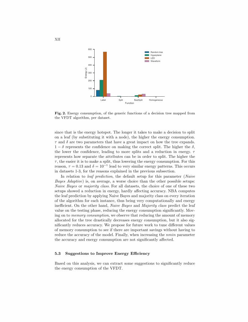
Fig. 2. Energy consumption, of the generic functions of a decision tree mapped fromthe VFDT algorithm, per dataset.

since that is the energy hotspot. The longer it takes to make a decision to spliton a leaf (by substituting it with a node), the higher the energy consumption.τ and δ are two parameters that have a great impact on how the tree expands.1 − δ represents the confidence on making the correct split. The higher the δ,the lower the confidence, leading to more splits and a reduction in energy. τrepresents how separate the attributes can be in order to split. The higher theτ , the easier it is to make a split, thus lowering the energy consumption. For thisreason, τ = 0.13 and δ = 10−1 lead to very similar energy patterns. This occursin datasets 1-3, for the reasons explained in the previous subsection.

In relation to leaf prediction, the default setup for this parameter (NaiveBayes Adaptive) is, on average, a worse choice than the other possible setups:Naive Bayes or majority class. For all datasets, the choice of one of these twosetups showed a reduction in energy, hardly affecting accuracy. NBA computesthe leaf prediction by applying Naive Bayes and majority class on every iterationof the algorithm for each instance, thus being very computationally and energyinefficient. On the other hand, Naive Bayes and Majority class predict the leafvalue on the testing phase, reducing the energy consumption significantly. Mov-ing on to memory consumption, we observe that reducing the amount of memoryallocated for the tree drastically decreases energy consumption, but it also sig-nificantly reduces accuracy. We propose for future work to tune different valuesof memory consumption to see if there are important savings without having toreduce the accuracy of the model. Finally, when increasing the nmin parameterthe accuracy and energy consumption are not significantly affected.

5.3 Suggestions to Improve Energy Efficiency

Based on this analysis, we can extract some suggestions to significantly reducethe energy consumption of the VFDT.

XIII

learnFromInstance_NBA()

filterInstanceToLeaf()

newNumericClassObserver()

learnFromInstance_UpStatistics()

getBestSplitSuggestions()

0

50

100

150

200

Ene

rgy

(J)

Fig. 3. Five functions with highest energy consumption.

– Avoiding using the parameter Naive Bayes Adaptive since it marginally in-creases accuracy and it consumes a lot of energy. The reason is that NaiveBayes and majority class are computed every time an instance is processed.

– Splitting the leaf into a node is more energy efficient than delaying the split,since updating the statistics at the leaves that have already observed manyinstances is very expensive.

– Increasing the δ and τ has positive effects on energy consumption, creatingmore splits and avoiding delaying the splits.

– If the data is numerical and complicated to keep track of, delaying the splitscan be more energy efficient.

6 Conclusions and Future Work

The aim of this paper is to profile the energy consumption of the Very FastDecision Tree algorithm. To achieve that, we have presented the following: (i)a methodology that profiles the energy consumption of decision trees at thefunction level, (ii) an experiment that uses this methodology to discover the mostenergy consuming functions of the VFDT, (iii) a thorough analysis to understandthe reasons behind the functions energy consumption, and (iv) which parametersettings decrease the energy consumption of such functions.

The analysis of the results show that the functions responsible for the labelingof the decision tree are the main energy hotspots. Specifically, updating thestatistics in the leaves and predicting the class at the leaf with parameter NBAare the main reasons for the amount of energy consumed in the algorithm. Theenergy consumption in labeling is significantly reduced if there are more splitson the leaves, rather than delaying the splitting to gain a higher confidence.Additionally, the results show that the energy can be reduced up to a 74.3% bytuning the parameters of the VFDT.

XIV

0 200 400 600 800 1000Energy (J)

75

80

85

90

95

100

Acc

urac

y (%

)

DatasetRandom treeHyperplaneLEDWaveform

Fig. 4. Trade-off between accuracy and energy for all setups and datasets. Each datasethas a different pattern of energy consumption. The random tree has the highest accu-racy and lowest energy consumption.

The planned future work is to make an energy efficient extension of the VFDTwith the knowledge extracted from this study. We will also investigate in moredepth different parameter combinations to see if energy can be reduced further.We also plan to compare the predictive performance and the energy consumptionof other tree learners with the VFDT.

Acknowledgments. This work is part of the research project ”Scalable resource-efficient systems for big data analytics” funded by the Knowledge Foundation(grant: 20140032) in Sweden.

References

1. Ahmed, N.K., Atiya, A.F., Gayar, N.E., El-Shishiny, H.: An empirical comparisonof machine learning models for time series forecasting. Econometric Reviews 29(5-6), 594–621 (2010)

2. Bifet, A., Holmes, G., Kirkby, R., Pfahringer, B.: MOA: Massive online analysis.The Journal of Machine Learning Research 11, 1601–1604 (2010)

3. Caruana, R., Niculescu-Mizil, A.: An empirical comparison of supervised learn-ing algorithms. In: Proceedings of the 23rd international conference on Machinelearning. pp. 161–168. ACM (2006)

4. De Francisci Morales, G.: Samoa: A platform for mining big data streams. In:Proceedings of the 22nd International Conference on World Wide Web. pp. 777–778. ACM (2013)

XV

5. Demirci, M.: A survey of machine learning applications for energy-efficient resourcemanagement in cloud computing environments. In: IEEE 14th International Con-ference on Machine Learning and Applications (ICMLA). pp. 1185–1190 (2015)

6. Domingos, P., Hulten, G.: Mining high-speed data streams. In: Proceedings ofthe 6th ACM SIGKDD international conference on Knowledge discovery and datamining. pp. 71–80 (2000)

7. Flach, P.: Machine learning: the art and science of algorithms that make sense ofdata. Cambridge University Press (2012)

8. Freire, A., Macdonald, C., Tonellotto, N., Ounis, I., Cacheda, F.: A self-adaptinglatency/power tradeoff model for replicated search engines. In: 7th ACM interna-tional conference on Web search and data mining. pp. 13–22 (2014)

9. Gama, J., Rocha, R., Medas, P.: Accurate decision trees for mining high-speed datastreams. In: Proceedings of the ninth ACM SIGKDD International Conference onKnowledge Discovery and Data Mining. pp. 523–528. ACM (2003)

10. Hoeffding, W.: Probability inequalities for sums of bounded random variables.Journal of the American statistical association 58(301), 13–30 (1963)

11. Hooper, A.: Green computing. Communication of the ACM 51(10), 11–13 (2008)12. Hulten, G., Spencer, L., Domingos, P.: Mining time-changing data streams. In:

Proceedings of the seventh ACM SIGKDD international conference on Knowledgediscovery and data mining. pp. 97–106 (2001)

13. King, R.D., Feng, C., Sutherland, A.: Statlog: comparison of classification algo-rithms on large real-world problems. Applied Artificial Intelligence an InternationalJournal 9(3), 289–333 (1995)

14. Kirkby, R.B.: Improving hoeffding trees. Ph.D. thesis, The University of Waikato(2007)

15. Kourtellis, N., Morales, G.D.F., Bifet, A., Murdopo, A.: VHT: Vertical HoeffdingTree. arXiv preprint arXiv:1607.08325 (2016)

16. Mart́ın, E.G., Lavesson, N., Grahn, H.: Energy efficiency in data stream mining.In: Proceedings of the 2015 IEEE/ACM International Conference on Advances inSocial Networks Analysis and Mining 2015. pp. 1125–1132. ACM (2015)

17. Mart́ın, E.G., Lavesson, N., Grahn, H.: Energy efficiency analysis of the VeryFast Decision Tree algorithm. In: Missaoui, R., Abdessalem, T., Latapy, M. (eds.)Trends in Social Network Analysis - Information Propagation, User Behavior Mod-elling, Forecasting, and Vulnerability Assessment. (To appear in April 2017) (2016)

18. Murdopo, A.: Distributed decision tree learning for mining big data streams (2013)19. Murugesan, S.: Harnessing green it: Principles and practices. IT professional 10(1),

24–33 (2008)20. Noureddine, A., Rouvoy, R., Seinturier, L.: Monitoring energy hotspots in software.

Automated Software Engineering 22(3), 291–332 (2015)21. Reams, C.: Modelling energy efficiency for computation. Ph.D. thesis, University

of Cambridge (2012)22. Wu, X., Zhu, X., Wu, G.Q., Ding, W.: Data mining with big data. IEEE Transac-

tions on Knowledge and Data Engineering 26(1), 97–107 (2014)23. Yang, T.J., Chen, Y.H., Sze, V.: Designing energy-efficient convolutional neural

networks using energy-aware pruning. arXiv preprint arXiv:1611.05128 (2016)