
Post- and Pre-stack attribute analysis and inversion of...
154
Post- and Pre-stack attribute analysis and inversion of Blackfoot 3Dseismic dataset A Thesis Submitted to the College of Graduate Studies and Research in Partial Fulfillment of the Requirements for the degree of MASTER OF SCIENCE in Geophysics Department of Geological Sciences University of Saskatchewan Saskatoon by Abdulsalam Swisi © Copyright 2009 Abdulsalam Swisi, October 2009. All Rights Reserved
Transcript of Post- and Pre-stack attribute analysis and inversion of...

Post- and Pre-stack attribute analysis and inversion of
Blackfoot 3Dseismic dataset
A Thesis Submitted to the College of
Graduate Studies and Research
in Partial Fulfillment of the
Requirements for the degree of
MASTER OF SCIENCE
in
Geophysics
Department of Geological Sciences
University of Saskatchewan
Saskatoon
by
Abdulsalam Swisi
© Copyright 2009 Abdulsalam Swisi, October 2009. All Rights Reserved

i
PERMISSION TO USE
In presenting this thesis in partial fulfillment of the requirements for a postgraduate degree
from the University of Saskatchewan, I agree that the libraries of this University may make
it freely available for inspection. I further agree that permission for copying of this thesis in
any manner, in whole or in part, for scholarly purposes may be granted by the professor
who supervised my thesis work or, in his absence, by the department Head of the Depart-
ment or the Dean of the College in which my thesis work was done. It is understood that
any copy or publication or use of this thesis or parts thereof for financial gain shall not be
allowed without my written permission. It is also understood that due recognition shall be
given to me and to the University of Saskatchewan in any use which may be made of any
material in my thesis.
Request for permission to copy or to make other use of material in this thesis in whole
or part should be addressed to:
Head of the Department of Geological Sciences
114 Science Place
University of Saskatchewan
Saskatoon, Saskatchewan S7N 5E2

ii
Abstract
The objective of this research is comparative analysis of several standard and one
new seismic post- and pre-stack inversion methods and Amplitude Variation with Offset
(AVO) attribute analysis in application to the CREWES Blackfoot 3D dataset. To prepare
the data to the inversion, I start with processing the dataset by using ProMAX software.
This processing, in general, includes static and refraction corrections, velocity analysis and
stacking the data. The results show good quality images, which are suitable for inversion.
Five types of inversion methods are applied to the dataset and compared. Three of
these methods produce solutions for the post-stack Acoustic Impedance (AI) and are per-
formed by using the industry-standard Hampson-Russell software. The fourth method uses
our in-house algorithm called SILC and implemented in IGeoS seismic processing system.
In the fifth approach, the pre-stack gathers are inverted for elastic impedance by range-
limited stacking of the common-midpoint (CMP) gathers in offsets and/or angles and then
performing independent inversion of angle stack. Further, simultaneous inversion is ap-
plied to pre-stack seismic data to invert for both the P- and S-wave impedances. These im-
pedances are used to extract the Lamé parameters multiplied by density (LMR), and used
to extract the ratios between the P- and S-wave velocities. In addition, CMP gathers are
used to produce AVO attribute images, which are good indicators of gas reservoirs. Fi-
nally, the results of the different inversion techniques are interpreted and correlated with
well-log data and used to characterize the reservoir.
The different inversion results show clearly the reservoir with its related low im-
pedance within the channel. The post-stack inversion gives the best results; in particular,
the model-based inversion shows smoothed images of it while SILC provides a different,
higher-resolution image. The elastic impedance also gives results similar to the post-stack
inversion. Pre-stack inversion and AVO attributes give reasonable results in cross sections
near the center of study area. In other areas, performance of pre-stack inversion is poorer,
apparently because of reflection aperture limitations.

iii
ACKNOWLEDGMENTS
This research was made possible through financial support from the Libyan Gov-
ernment. I express my gratitude to my thesis supervisor Dr. Igor Morozov for his invalu-
able advice, encouragement, support, and guidance. My thanks also go to committee mem-
bers Drs. Kevin Ansdell, Jim Merriam, Samuel Butler and the external examiner Dr. Brian
Russell. Thanks also extend to Dr. JingFeng Ma for his advice, encouragement and sup-
port. I also would like to thank Brian Reilkoff for computing services. This work was fa-
cilitated by software grants from Landmark Graphics Corporation (Halliburton) and
Hampson-Russell Limited (CGG/Veritas). I am particularly grateful to Hampson-Russell
for providing data examples and organizing training in seismic inversion at the University
of Saskatchewan.

iv
SYMBOLS AND ABBREVIATIONS
Symbol Definition
2D, 2-D
3C
3D, 3-D
A
AGC
AI
AVA
AVO
B
C
CCP
CMP
DMO
EI
F/X
FF
FK, f-k
FXY
GLI3D
IGeoS
H-R
LMR
LR
MR
NMO
QC
R
RMS
SILC
VP
Two-Dimensional
Three-Component
Three-Dimensional
Intercept (AVO attribute)
Automatic Gain Control (trace equalization proce-
dure)
Acoustic Impedance; in simultaneous inversion, also
denoted ZP
Amplitude Variation with Angle
Amplitude Variation with Offset
Gradient (AVO attribute)
Curvature (AVO attribute)
Common Conversion Point
Common Mid- Point
Dip Move-Out
Elastic Impedance
Frequency-space (in 2D)
Fluid Factor
Frequency-wavenumber
Frequency-space (in 3D)
Generalized Linear Inverse 3D (refraction statics
program by Hampson-Russell)
Integrated GeoScience (software package)
Hampson-Russell
Lambda, Mu, -Rho (, , ) –Lamé parameters
attribute
attribute
Normal Move-Out
Quality Control
Reflectivity
Root-Mean-Square
Poisson‟s ratio
Seismic Inversion of by well-Log Calibration
P-wave velocity

v
VS
VSP
ZP
ZS
Ρ
S-wave velocity
Vertical Seismic Profiling
P-wave (acoustic) impedance, also denoted AI
S-wave impedance
Density

vi
CONTENTS
PERMISSION TO USE .......................................................................................................... i
Abstract ............................................................................................................................. ii
ACKNOWLEDGMENTS..................................................................................................... iii
SYMBOLS AND ABBREVIATIONS ................................................................................ iv
LIST OF TABLES............................................................................................................... viii
1 Introduction ....................................................................................................................... 1
1.1 Use of impedance and AVO attributes in interpretation ...................................... 1
1.2 Objectives and structure of this thesis ................................................................... 3
1.3 Blackfoot 3C-3D dataset overview ....................................................................... 4
Source Parameters .................................................................................................. 8
Receiver parameters ............................................................................................... 8
1.4 Geological background ........................................................................................ 10
1.5 Seismic data processing ....................................................................................... 12
2 Methods ........................................................................................................................... 22
2.1 Pre-stack AVO attributes ..................................................................................... 22
2.2 Post-stack seismic inversion ................................................................................ 31
2.3 Elastic Impedance ................................................................................................. 45
2.4 Pre-stack inversion (simultaneous) ..................................................................... 48
3 Inversion and AVO attributes in Blackfoot 3D seismic dataset .................................. 51
3.1 Inversion of post-stack seismic data.................................................................... 52
3.2 Inversion for Elastic Impedance .......................................................................... 76
3.3 Inversion of pre-stack seismic data (“simultaneous inversion”) ....................... 88
3.4 Elastic rock parameters (, , ρ) and VP/VS ratios .............................................. 98
3.5 AVO attributes from Blackfoot CMP gathers .................................................. 101
4 Results and discussion.................................................................................................. 107

vii
4.1 Conclusions ......................................................................................................... 130
4.2 Suggestions for future research ......................................................................... 133
REFERENCES ............................................................................................................. 135

viii
LIST OF TABLES
Table 1.3.1. Pulsonic‟s vertical processing flow ...................................................................... 6
Table 1.3.2. Pulsonic‟s radial flow processing ......................................................................... 6
Table 1.3.3. Blackfoot 3D acquisition parameters (Glauconitic patch) .................................. 8
Table 1.5.1 Seismic data processing steps .............................................................................. 13
Table 3.1. Table of the Blackfoot area wells with, P-wave log, S-wave log and density logs
.................................................................................................................................................... 51
Table 3.2. Correlation between the synthetic trace and real trace at well locations using the
statistical and full wavelets ...................................................................................................... 54
LIST OF FIGURES
Figure 1.3.1. Location of Blackfoot area .................................................................................. 5
Figure 1.3.2. Map of Blackfoot surveys showing shot points of the full 3C-3D survey,
selected wells and a previous broad-band line (Zhang, 1996). ................................................ 7
Figure 1.3.3. Base map of shots (*), receivers (+) and CMP (×) used in the Blackfoot area.
...................................................................................................................................................... 9
Figure 1.3.4. CDP fold map. The fold number is the largest (142) at the centre and
decreases to the edges............................................................................................................... 10
Figure 1.4.1. Stratigraphic column of Cretaceous rocks in the Blackfoot area. ................... 12
Figure 1.5.1. Weathering layer with static corrections for cross line (145). Blue colour
shows the weathering layer model in the earth model. In upper plot, pink line shows the
receiver statics, and light blue – shot statics derived from this model. ................................. 14
Figure 1.5.2. Selected shot record before and after band-bass filter. Note the low-frequency
ground-roll waves are attenuated by this filtering. ................................................................. 15
Figure 1.5.3. Velocity analysis of a CMP gather. Left: velocity spectrum; middle: CMP
gather with offset; right: velocity analysis functions. ............................................................ 16
Figure 1.5.4. CDP gathers before (left) and after the NMO correction (right). .................... 17
Figure 1.5.5. Base map of the area sorted into in-line and cross-line sections, In-line
numbers range from 47 to 126 and cross-line numbers range from 88 to 205. .................... 18

ix
Figure 1.5.6. In-line and cross-line sections crossing the channel where the reservoir is
expected. The position of the Glauconitic channel is indicated. ........................................... 19
Figure 1.5.7. RMS Amplitude map at time slice of 1065 ms. Note the change from high
positive amplitude to high negative amplitude in the Glauconitic channel. ......................... 20
Figure 1.5.8. Time structure map of two horizons. Left: the top Manville above the
reservoir; right: the Mississippian carbonate beneath the reservoir. Locations of the wells
are also shown. .......................................................................................................................... 21
Figure 2.1.1 Notation used in eq. (2. 1.1). .............................................................................. 23
Figure 2.1.2 Amplitudes extracted from CMP gather are positive and is increasing with
offset for Class III gas sandstone. A and B are the intercept and slope of the amplitude
dependence on sin2, respectively. ........................................................................................ 24
Figure 2.1.3 Rutherford/Williams AVO classifications for the top of gas sands modified
from (Rutherford/Williams (1989)) ......................................................................................... 27
Figure 2.1.4 Mudrock lines for a range of values of the Vp/Vs ratio and Gardner‟s equation
on AVO intercept (A) and gradient (B) cross plot modified from (Castagna, 1998). .......... 28
Figure 2.1.5 Four possible anomalous classes in an AVO intercept (A) and gradient (B)
cross-plot. Reflections from the top of a gas-sand reservoir tend to fall below the
background trend, while bottom of the gas-sand reflections tend to fall above the
background trend redraw from (Castagna, 1998). .................................................................. 28
Figure 2.1.6. Interpretation of and cross plot is improved in gas well modified from
(Goodway,1997) ....................................................................................................................... 31
Figure 2.2.1. Concept of the Acoustic Impedance inversion. Red arrows show the forward
modelling while black arrows indicate the inversion. ............................................................ 32
Figure 2.2.2. Initial model derived from an AI log by using high-cut filtering. ................... 36
Figure 2.2.3. The inverted band-limited trace is added to the filtered model to obtain the
final inversion. .......................................................................................................................... 37
Figure 2.2.4. Blocky model derived from an impedance log................................................. 38
Figure 2.2.5. Convolution between a wavelet and blocky model to produce synthetic trace
and compare it with seismic trace. ........................................................................................... 39
Figure 2.2.6. AI from all wells (blue), one selected well (pink) and frequency on log-log
scale. .......................................................................................................................................... 40

x
Figure 2.2.7. Seismic spectra near the wells (blue). Red line corresponds to the f-𝜃 AI
spectrum derived in Figure 2.6. The operator spectrum (black) is the ratio of these two
spectra. ....................................................................................................................................... 41
Figure 2.2.8. Frequency spectrum of the operator (right) and its time response (left). ........ 41
Figure 2.2.9. Schematic diagram of the SILC inversion method in application to AI. ........ 43
Figure 2.2. 10. Principles of the scaling in the SILC inversion between seismic band and
well log band. ............................................................................................................................ 44
Figure 2.2. 11. SILC inversion steps from building AI, filtering AI and calculate time-
variant amplitude scale. ............................................................................................................ 44
Figure 2.3.1. Compared to AI, EI (30) shows a steeper decrease with increasing oil ........ 46
Figure 2.4.1. Cross plot between ln (ZP) and ln(ZS) (right) and ln(ZP) and ln(ρ). It indicate
that ZS and ρ are the linearly related to Zp; ∆𝑙𝑆 𝑎𝑛𝑑 ∆𝑙𝐷 indicate the devitation away from
background trend(red line) in case of fluid anomalies (CGG VERITAS workshop, 2008).
.................................................................................................................................................... 49
Figure 2.4.2. CMP gather showing the amplitude as a function of angle as described in
Fatti‟s ......................................................................................................................................... 50
Figure 3.1.1. Statistical wavelet extracted from seismic data in the time domain (left) and
frequency domain (right). Note that the wavelet is symmetrical in time and has zero phase.
.................................................................................................................................................... 53
Figure 3.1.2. Correlation at well 1-8 by using the statistical wavelet. The correlation level
is 84%. ....................................................................................................................................... 55
Figure 3.1.3. Full wavelet in the time (left) and frequency (right) domains extracted by
using well 14-9 and seismic data. Compare to Figure 3.1.1. ................................................. 56
Figure 3.1.4. Correlation at well 1-8 using the full wavelet. The correlation coefficient is
88%. Compare to Figure 3.1.2. ................................................................................................ 57
Figure 3.1.5. Seismic section showing the horizons used for interpolations and inversion.59
Figure 3.1.6. Stacked seismic section (left) and its frequency spectrum (right). Note that
there is no data below 10 Hz. ................................................................................................... 59
Figure 3.1.7. Cross section of unfiltered initial model impedance derived from well-log
interpolation. ............................................................................................................................. 60

xi
Figure 3.1.8. Cross-section of filtered initial model impedance derived from well-log
interpolation. ............................................................................................................................. 60
Figure 3.1.9. RMS average impedance of initial model indicated in slice at time 1065 ms,
for unfiltered (left) and filtered (right). ................................................................................... 61
Figure 3.1.10. Inverted result (red) using the band-limited algorithm compared with the
original log (blue) at the well 1-17. Note that the impedance of the log is filtered using a
high-cut filter (50-60 Hz). ........................................................................................................ 63
Figure 3.1.11. Inverted synthetic traces correlated with seismic data (top) and the average
RMS errors between the original logs and inverted result (bottom). .................................... 64
Figure 3.1.12. Cross-section of band-limited inversion results. Note the low impedance
around 1065 ms (ellipse). ......................................................................................................... 64
Figure 3.1.13. Time slice of the RMS average impedance result at 1065 ms from the band-
limited inversion. ...................................................................................................................... 65
Figure 3.1.14. Inverted result using H-R model-based algorithm compared to the original
log at well 4-16. ........................................................................................................................ 67
Figure 3.1.15. Top: Correlation of the inverted synthetic and real seismic trace.
Bottom:RMS errors between the original logs and inverted results for all wells.......68
Figure 3.1.1. Cross-section of model based-inversion results. Note the low impedances
around 1065 ms (ellipse)......................................................................................................69
Figure 3.1.17. Slice at time 1065 ms from the model-based inversion in the study area. .. 69
Figure 3.1.18. Operator used in coloured inversion in the time (left) and frequency (right)
domains. .................................................................................................................................... 70
Figure 3.1.19. Inverted result using coloured algorithm compared with the original log at
well 1-17. ................................................................................................................................... 71
Figure 3.1.20. Inverted synthetic correlation and errors between the original logs and
inverted results from all wells. ................................................................................................. 72
Figure 3.1.21. Cross-section of the coloured inversion result. Note the low impedances
around 1065 ms. ........................................................................................................................ 72
Figure 3.1.22. Slice at time 1065 ms across the coloured-inversion result for the study area.
.................................................................................................................................................... 73
Figure 3.1.23. Cross-section of the SILC inversion result. .................................................... 74

xii
Figure 3.1.24. Slice of the RMS average impedance of the SILC AI at time 1065 ms. ...... 75
Figure 3.2.1. CMP gathers shown as offset gathers (top) and angle gathers (bottom). ....... 77
Figure 3.2.3. Statistical wavelets constructed from near angle section stack (left) and far
angle section stack (right). ....................................................................................................... 79
Figure 3.2.4. Initial models constructed from wells and seismic horizons: near-angle (left)
and far-angle (right). ................................................................................................................. 80
Figure 3.2.5. Quality control at well location to compare the band-limited EI result the
well: left: near-offset, right: far-offset. Curves and notation as in Figure 3.1.10. .............. 81
Figure 3.2.6. For the band-limited near-angle inversion: red: correlation coefficients of the
inversion result to to seismic traces; blue: errors between the original logs and inverted
results for all wells (blue). ........................................................................................................ 82
Figure 3.2.7. For the band-limited far-angle inversion: red: correlation coefficients of the
inversion result to to seismic traces; blue: errors between the original logs and inverted
results for all wells (blue). ........................................................................................................ 82
Figure 3.2.8. Two cross-sections of the EI using band limited method: near inversion (top)
and far inversion (bottom). ....................................................................................................... 83
Figure 3.2.9. Slices of EI are taken at time 1065 ms for band-limited method: near-angle
(left) and far-angle (right). ....................................................................................................... 84
Figure 3.2.10. Quality control applied at well location to compare elastic impedance result
to elastic at the well using model-based method, near elastic impedance (left) and far
elastic impedance (right). ......................................................................................................... 85
Figure 3.2.11. Quality control of the near-angle, model-based EI inversion: Top:
correlation of the predicted and real seismic reflectivity; Bottom: RMS errors between the
well--log and inverted EI.......................................................................................................... 86
Figure 3.2.12. Quality control of the far-angle, model-based EI inversion: Top: correlation
of the predicted and real seismic reflectivity; Bottom: RMS errors between the well--log
and inverted EI. ......................................................................................................................... 86
Figure 3.2.13. EI cross-sections of the EI using the model-based method: near-angle (top)
and far-angle (bottom). P-wave log in well 8-8 is shown in black. ....................................... 87
Figure 3.2.14. Slices of EI at time 1065 ms for model-based inversion: near-angle (left)
and far-angle (right). ................................................................................................................. 88

xiii
Figure 3.3.1. Top: CMP gathers; bottom: the initial AI model for inversion. ...................... 90
Figure 3.3.2. Well-log data (coloured dots) and the interpreted background relationships
between ln(ZP), ln(ZS), and ln() (lines) using all wells in the area. These trends were used
to calculate the coefficients (k, kc, m, and mc)......................................................................... 91
Figure 3.3.3. Left: quality control applied to compare the inverted of P-impedance, S-
impedance and VP/VS ratio to the corresponding parameters of the well. Right:
comparison of the CMP gather data to the synthetic CMP gather constructed from the
inversion result, and the prediction error. ............................................................................... 93
Figure 3.3.4. Red: correlation coefficients between the synthetic seismic traces using the
inversion result and the corresponding gathers in the seismic data. Blue: RMS errors in ZP
between the original logs and inverted results for all wells, ZP; purple: similar errors for ZS.
.................................................................................................................................................... 94
Figure 3.3.5. Cross-sections of the P-impedance (ZP; top) and S-impedance (ZS; bottom)
inversion results. ....................................................................................................................... 96
Figure 3.3.6. Top: Selected NMO-corrected CMP gathers from the seismic data; Middle:
Synthetic gathers constructed from the inversion result; Bottom: the error (differences)
between the real and synthetic CMP gathers. Red line shows the p-wave log in well # 8-8.
.................................................................................................................................................... 97
Figure 3.3.7. Time-slice of ZP (left) and ZS (right) inversion at 1065 ms. Ellipse shows the
channel with low P- impedance and relatively high S-impedance. ....................................... 98
Figure 3.4.1. Cross-section of the LR attribute resulting from the simultaneous inversion.
Cross-section of the MR attribute. ........................................................................................... 99
Figure 3.4.2. Cross-section of the VP/VS ratio derived from simultaneous inversion......... 100
Figure 3.4.3. Left: Time slice of LR inversion at 1065 ms. Right: time slice of MR
inversion at 1065 ms. The ellipse show the low LR (left) and high MR in the channel. ... 100
Figure 3.4.4. Time slice of VP/VS inversion result at 1065 ms time. The ellipse shows a
zone of low VP/VS within the channel. .................................................................................. 101
Figure 3.5.1. CMP gathers (top) and the variation of reflection amplitude with angles
(bottom) at horizon a1. Horizons are shown in Figure 3.1.5. .............................................. 102
Figure 3.5.2. Intercepts A (top) and gradients B (bottom) in a line crossing gas well #1-17.
Black line shows the P-wave log in the well. ....................................................................... 103

xiv
Figure 3.5.3. The same section as in Figure 3.5.2 showing product AB. ............................ 104
Figure 3.5.4. Poisson‟s ratio A+B section at the gas well # 1-17. ....................................... 104
Figure 3.5.5. Scaled S-wave reflectivity A-B section near gas well # 1-17. ....................... 105
Figure 3.5. 6 P-wave reflectivities (RP) , used to extract the Fluid Factor (FF) near gas well
#1-17. ....................................................................................................................................... 105
Figure 3.5.7. S-wave reflectivities (RS) , used to extract the Fluid Factor (FF) near gas well
#1-17. ....................................................................................................................................... 106
Figure 3.5.8. Fluid factor section near gas well # 1-17. ....................................................... 106
Figure 4.1. Cross-section of the AI across the channel, by using the band-limited (left) and
model-based (right) inversion. Ovals indicate the interpreted zone of low AI related to the
reservoir. .................................................................................................................................. 109
Figure 4.2. Cross-section of the AI across the channel, by using coloured (left) and SILC
(right) inversion. Ovals indicate the zone of low AI related to the reservoir. ................... 109
Figure 4.3. Impedance slices at 1070 ms time depth: band-limited (left) and model-based
(right). The low-impedance zone is seen clearly in the channel. Purple colour corresponds
to the Mississippian carbonates. ............................................................................................ 111
Figure 4.4. Impedance slices at 1070 ms time depth: coloured (left) and SILC (right). The
low-impedance zones are shown clearly in the channel. Purple colour corresponds to the
Mississippian carbonates. ....................................................................................................... 112
Figure 4. 5. Cross-section of the AI across the channel with average values from 8300
(m/s)·(g/cc) to (m/s)·(g/cc)11800. .......................................................................................... 113
Figure 4. 6. Impedance slices with new average impedance values: at 1065 ms time depth
with average of 10 ms time window (left) and 1070 ms time depth (right). The low-
impedance zones are shown more clearly in the channel..................................................... 114
Figure 4.7. Cross-sections of the near-offset (left) and far-offset (right) EI across the
channel, using the band-limited inversion method ............................................................... 115
Figure 4.8. Cross-section of the EI across the channel using the model-based method at
near (left) and far angles (right). ............................................................................................ 116
Figure 4.9. Near-offset (left) and far-offset (right) Elastic Impedance slice at 1070 ms time
depth using the band-limited inversion. The low-impedance areas in the channel are
indicated by ellipses................................................................................................................ 117

xv
Figure 4.10. Elastic impedance slice at 1070 ms time depth using mode-based, near (left)
and far (right). The low-impedance zones in the channel are seen clearly (ellipses). ........ 118
Figure 4.11. P-impedance (top) and S-impedance (bottom) near the gas reservoir. Ellipses
indicate the zone of low P-impedances related to the gas reservoir (above) and relatively
high S-impedance (bottom). ................................................................................................... 119
Figure 4.12. P-impedance (left) and S-impedance (right) slices at 1070 ms time depth. The
ellipse indicates the channel. The low P-impedance and relatively high S-impedance are
visible in the channel. ............................................................................................................. 121
Figure 4.13. (top) and (bottom) attributes near the reservoir. Ellipses indicate the gas
reservoir. .................................................................................................................................. 122
Figure 4.14. VP/VS ratios appear to emphasize the reservoir best. Ellipse indicates the gas
reservoir. .................................................................................................................................. 123
Figure 4.15. Slices of LMR parameters 1070-ms time-depth: (left) and (right). The
ellipses indicate the channel area. The low- and high- anomalies are shown clearly
within the channel. .................................................................................................................. 124
Figure 4.16. VP/VS ratio distribution at 1070-ms time-depth. Note the low VP/VS ratio
within the channel. .................................................................................................................. 125
Figure 4.17. The AVO intercept A (top) and gradient B (bottom) sections indicate the gas
reservoir. Note that the gradient appears to show a better result (more localized
horizontally) than the intercept. ............................................................................................. 127
Figure 4.18. AVO product (AB) indicates the top and the base of the reservoir. ............... 128
Figure 4.19. Poisson‟s ratio at the top and base of the gas reservoir. ................................. 128
Figure 4.20. S-wave reflectivity (A-B) indicates the top and bottom of the reservoir........ 129
Figure 4.121. Fluid factor (FF) indicates the deviation from Castagna‟s equation at top and
bottom of the reservoir. .......................................................................................................... 129
Figure 4. 22. Valley of the Blackfoot area extracted from well information (Lawton, 1995).
.................................................................................................................................................. 131

1
1 Introduction
1.1 Use of impedance and AVO attributes in interpretation
Since the 1970‟s, Acoustic Impedance (AI) has become a primary quantity used in
seismic reflectivity inversion and interpretation (Lindseth, 1979). The key attractive prop-
erty making AI so useful is its direct correlation with rock properties measured in the labo-
ratory and in the field, since it is the product of density and acoustic velocity. By contrast
to seismic reflectivity, which occurs at the contacts of contrasting strata, AI takes on con-
stant values within rock layers, allowing a straightforward and intuitive correlation with
geology and stratigraphy.
The impedance is extracted from seismic reflection data by a process usually called
inversion. Seismic inversion tries to transform the spiked seismic reflectivity at geological
boundaries (caused by changes in the lithology or physical state) into meaningful mechani-
cal layer properties (impedances). In the acoustic (P-wave) case, the inversion algorithm
transforms the reflection amplitudes into AI, which is the product of density and P-wave
velocity, AI= ρVP. In well-log measurements, both of these properties can be measured, and
therefore impedance logs can be obtained and directly compared to the seismic AI.
Through the process of seismic inversion, we can transform seismic sections to AI sec-
tions, which represent the lithological properties of the layers rather than interface proper-
ties. Therefore, transformation to AI simplifies the lithological and stratigraphic interpreta-
tion and plays an important role in seismic interpretation and reservoir characterization,
such as identification of fluid-filled and porous zones.
The AI is typically inverted from stacked seismic data, which approximate the
normal-incidence reflectivity. However, pre-stack Amplitude Variations with incidence
Angle (AVA) also contain a wealth of information about the mechanical properties of the
reflector. Ostrander (1982) sparked the initial interest in pre-stack seismic attributes when
he pointed out that gas-sand reflection coefficients change in an anomalous manner with
increasing offsets and showed how to utilize this behaviour as a direct hydrocarbon indica-
tor. The AVA method is generally, the Amplitude Variation with Offset (AVO) method,
and was further developed (Ostrander, 1982) to assist in identifying the fluid content of the

2
reservoir. The AVO method started with production of models and comparison of these
models to the common-offset stacks gathered from real seismic data (Russell and
Hampson, 1991). The Aki and Richards‟ (2002) equation for seismic reflectivity was com-
bined by Smith and Gidlow (1987) with mudrock line (Castagna et al., 1985) to emphasize
the anomalies in seismic data that could be useful indicators of hydrocarbon reservoirs.
Today, AVO analysis and inversion of seismic data are routinely used to derive
seismic attributes which are used as hydrocarbon indicators. Such attributes usually are:
the acoustic impedance (ZP = AI= ρVP), shear impedance (ZS = ρVS), elastic impedance
(EI), Lamé parameters (LMR) and the ratio of compressional- and shear-wave velocities
(VP/VS) (Singh, 2007). The elastic impedance is defined as an extension of the convolu-
tional model to non-zero incident angles (Connolly, 1999). The LMR attributes attempt
capturing the intrinsic mechanical properties of the rock, such as the products of their elas-
tic modules ( and ) with density (). From these attributes, we can derive the P- and S-
wave velocities and densities which can be further used to describe the properties of rock
matrix and pore fluid. Thus, from true-amplitude processing of seismic traces, we can ex-
tract the reflectivities and impedances, and by adding the measured velocities, the densi ty
can be further estimated.
In the AVO analysis, pre- and post-stack techniques should be carefully differenti-
ated (Russell, 1988). Post-stack seismic inversion methods use stacked (zero-offset) seis-
mic data to produce images of the AI in depth or time. Pre-stack (AVO) inversion uses the
variations of reflection amplitudes within the individual Common Midpoint Gathers
(CMP) in order to determine the complete set of elastic properties (VP, VS, ρ), or equiva-
lently, elastic constant properties (λ, μ, ρ) of the subsurface. From these properties, the
petrophysical properties and fluid/gas saturation may be further inferred. In addition, CMP
gathers can be used to directly invert for the P- and S-wave impedances and to extract
other attributes such as VP/VS ratios. Both of these methods depend on the theoretical rela-
tionships between the physical properties and the seismic amplitudes. In summary, varia-
tions of the amplitudes of post and pre-stack seismic data are valuable for hydrocarbon in-
vestigation, especially in relation to gas reservoirs.

3
1.2 Objectives and structure of this thesis
This project focuses on comparing several techniques used to identify and charac-
terize a thin reservoir in Blackfoot area by using 3D seismic dataset and geophysical logs
from eleven wells in the area. A new impedance inversion technique recently proposed by
Morozov and Ma (in press) called Seismic Inversion by well-Log Calibration (SILC) is
also applied to the seismic data and compared to the conventional techniques. The specific
objectives of this study are:
1. Process the seismic data and prepare them to inversion and AVO analysis. This re-
sults in:
a. Stacked data;
b. Range-limited stacked data;
c. CMP gathers for pre-stack inversion.
2. Identify and pick horizons.
3. Use correlation to tie between seismic and wells in the area.
4. By using post-stack data, apply inversion methods to extract the AI by using:
a. Model-based inversion;
b. Band-limited inversion (also called iterative or recursive);
c. Coloured inversion;
d. Seismic Inversion by well-Log Calibration (SILC).
5. From range-limited stacked data:
a. Perform elastic impedance for near and far angle stack.
6. From CMP gathers:
a. Apply simultaneous inversion to extract the P-impedance, S-impedance, VP/VS ratio
and LMR parameters;
b. Create volumes of attributes such as the AVO intercept (A), gradient (B) and Fluid
Factor (FF).
7. Visualize and interpret the images, correlate with the available well logs and known
gas reservoirs within the area.

4
Based on this comparative analysis, I make conclusions and recommendations re-
garding the effectiveness of the different attributes for identifying the gas reservoir and for
measuring its parameters.
This thesis is organized as follows. In Chapter 1, I give an introduction to the use of
impedance and AVO attributes in interpretation, as well as detailed objectives of the study,
an overview the Blackfoot 3C-3D dataset, and a description describe the geological back-
ground and a brief outline of the seismic data processing. Chapter 2 discusses the methods
and theories used in this research, such as the AVO attributes, post-stack inversion, elastic
impedance, pre-stack inversion and elastic parameters (λ, μ and ρ). Chapter 3 gives a fur-
ther discussion of the implementation of the methods and their parameters for the Blackfoot
3D dataset. Four post-stack AI methods and one pre-stack EI inversion methods are applied
to our seismic data in this Chapter. EI, AVO, and LMR attributes are also discussed in
Chapter 3. In Chapter 4, I present the results and discussions, as well as make conclusions
from this study and offer some suggestions for future research.
1.3 Blackfoot 3C-3D dataset overview
The Blackfoot field is located south-east of Strathmore, Alberta, Canada in Town-
ship 23, Range 23W4 (Figure1.3.1). Extensive seismic work has been done in this field by
Pan Canadian Petroleum and the CREWES (the Consortium for Research in Elastic-Wave
Exploration Seismology) project at the University of Calgary. The 3C-3D seismic dataset
was recorded in October 1996. The goal of this experiment was to demonstrate that 3C-3D
seismic data (P-P, P-S) can be used to enhance the conventional 3D P-wave structural and
stratigraphic images, to discriminate the lithology, and to study anisotropy (Lawton, 1996).
This survey was recorded in two overlapping patches: the first patch targeted the clastic
Glauconitic channel, and the second one went deeper to consider the reef-prone Beaverhill
lake carbonate. In the present study, we only consider the first patch, which focused on the
Glauconitic channel.

5
Figure 1.3.1. Location of Blackfoot area
The Blackfoot dataset was processed by Pulsonic Geophysical and Sensor Geo-
physical. Filtering and deconvolution was the initial test done on the data; and the band-
width of the data was found to be 5-90 Hz for the vertical-component data and 5-50 Hz for
horizontal data. The following two processing flows show the processing steps for the ver-
tical and horizontal data (Simin et al, 1996).

6
Table 1.3.1. Pulsonic’s vertical processing flow
SEG-D reformatted demultiplex input
Component separation
3D geometry assignment
Trace edits
Surface-consistent amplitude balance
Surface consistent deconvolution
Horizontal component rotation
Elevation and refraction statics
Residual surface-consistent statics
Asymptotic CCP macro-bin sort
Velocity analysis
3D NMO correction
Velocity specific filter
FK median filter
Trace mute
3D converted wave DMO
3D CCP bin stack
F/X migration
Spectral balance
FXY deconvolution
Band-pass filter
Time-variant scaling
Table 1.3.2. Pulsonic’s radial flow processing
SEG-D reformatted demultiplex input
Component separation
3D geometry assignment
Trace edits
Surface-consistent amplitude balance
Surface consistent deconvolution
Horizontal component rotation
Elevation and refraction statics
Residual surface-consistent statics
Asymptotic CCP macro-bin sort
Velocity analysis
3D NMO correction
Velocity-specific filter
FK median filter
Trace mute
3D converted wave DMO
3D CCP bin stack
F/X migration
Spectral balance
FXY deconvolution
Band-pass filter
Time-variant scaling
7
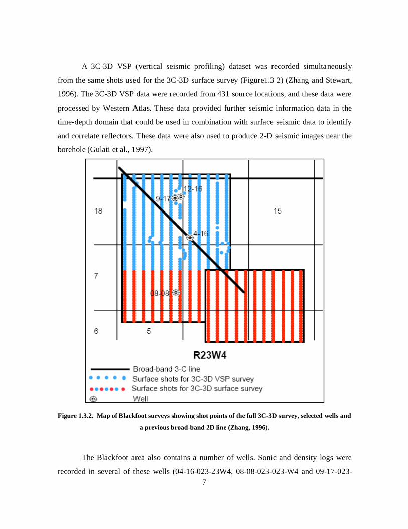
A 3C-3D VSP (vertical seismic profiling) dataset was recorded simultaneously
from the same shots used for the 3C-3D surface survey (Figure1.3 2) (Zhang and Stewart,
1996). The 3C-3D VSP data were recorded from 431 source locations, and these data were
processed by Western Atlas. These data provided further seismic information data in the
time-depth domain that could be used in combination with surface seismic data to identify
and correlate reflectors. These data were also used to produce 2-D seismic images near the
borehole (Gulati et al., 1997).
Figure 1.3.2. Map of Blackfoot surveys showing shot points of the full 3C-3D survey, selected wells and
a previous broad-band 2D line (Zhang, 1996).
The Blackfoot area also contains a number of wells. Sonic and density logs were
recorded in several of these wells (04-16-023-23W4, 08-08-023-023-W4 and 09-17-023-

8
23W4). Well 08-08-023-023-W4 is a multi zone-gas producer from the top channel and oil
from the base. Well-log data were used to correlate the seismic data and to guide the AVO
analysis and inversion.
From 1995, extensive research work was done on the Blackfoot field, primarily by
members of the CREWES project. Using the Blackfoot data, CREWES has produced sev-
eral reports in different research areas, such as AVO analysis, simultaneous P-P and P-S
inversion, processing, 3C-3D VSP and converted-wave seismic exploration (Xu and Ban-
croft, 1997; Larsen et al., 1998; Simin et al, 1996; Gulti et al., 1997; and Stewart et al.,
1999).
In this study, I only utilize the conventional (vertical-component) 3D seismic data
and eleven well-log datasets. Figure 1.3.3 shows the base map of the shots, receivers and
CMP of the Blackfoot area used in this study. The dataset contains 708 shots into a fixed
recording spread of 690 channels. The fold is 140 at the centre of the spread, as shown in
Figure 1.3.4. Acquisition parameters used in this patch are described in Table 1.3.3.
Table 1.3.3. Blackfoot 3D acquisition parameters (Glauconitic patch)
Source Parameters
Line orientation
Source interval
Source line interval
Number of source lines
Total number of source points
Source depth
North-South
60m
210m
12
708
18m
Receiver parameters
Line orientation
Receiver interval
Receiver line interval
Number of receiver lines
Total number of receiver points
Receiver depth
East-West
60m
255m
15
690
0.5m

9
Figure 1.3.3. Base map of shots (*), receivers (+) and CMPs (×) used in the Blackfoot area.

10
Figure 1.3.4. CDP fold map. The fold number is the largest (142) at the centre and decreases to the
edges of the survey.
1.4 Geological background
The following is a brief review of the geology in Blackfoot area. Our target is the
Glauconite Formation of the Lower Cretaceous which represents: sediment filled incised
valley. Glauconite Formation of the Lower Cretaceous represent the upper Manville Group

11
The thickness of the Glauconite sand varies up to 35meter at encounter depth 1550m where
is the reservoir depth. The grain size of the Glauconite Formation varies from fine to me-
dium.
In this field, eroded Mississippian carbonates are covered with Lower Cretaceous
sediments. These sediments are the Detrital member of variable thickness, while above this
Detrital member there are sheet and ribbon Sunburst sands. At a later time (Cretaceous),
marine transgression deposited brackish shales, limestones and quartz sands and silts to
build the Ostracod member. The Glauconitic member consists of shales and sands of lacus-
trian and channel origin. Within the channel, the sediments are subdivided into three units
corresponding to three phases of valley incision with different quality of sand deposited.
These three units may are not be encountered everywhere in the area. The reservoir in the
Blackfoot field is producing from the Glauconitic sand of the Lower Cretaceous Glauco-
nitic Formation, in which the porosities are up to 18% . Figure 1.4.1 (Margrave et al.,
1998) shows the stratigraphic column of the Blackfoot area. This field mainly produces oil
and gas in some wells. In more detail, the geology of the Blackfoot Field was well dis-
cussed by Miller et al. (1995).

12
Figure 1.4.1. Stratigraphic column of Cretaceous rocks in the Blackfoot area (Margrave et al., 1997).
1.5 Seismic data processing
ProMAX software was used for processing the Blackfoot 3D seismic data. The ini-
tial data loading and geometry set up was performed by Dr. Ma prior to the beginning of
this study. After this, trace editing was applied to remove bad traces and to correct traces
with reverse polarities. In addition, true amplitude recovery was performed to compensate
for the loss of amplitudes caused by wave divergence away from the sources. The remain-
ing seismic processing steps were: inversion for statics correction, noise filtering, velocity
analysis and stacking, as shown in Table 1.5.1.

13
Table 1.5.1. Seismic data processing steps
# Operation Purpose
1 3D GEOMETRY ASSIGNMENT
(performed by Dr. Jinfeng Ma)
Providing the geographic reference.
2 TRACE EDITS Removing bad traces, reversing polarity as necessary,
and muting.
3 TRUE AMPLITUDE RECOVERY To recover the loss of amplitude as the wave divergence
4 ELEVATION AND REFRACTION STAT-
ICS
Time correction for shallow subsurface
5 BAND-PASS FILTER Attenuating the ground roll in shot gathers
6 VELOCITY ANALYSIS Extract RMS velocity for NMO correction
7 3D NMO CORRECTION Removal of reflection time moveout.
8 3D CMP stack Increasing signal to noise ratio.
9 AGC ( Automatic gain control) and DIS-
PLAY
Increase the amplitude for display
10 F-X deconvolution Reducing random noise and improving image coherency
First, elevation and refraction static corrections were applied by using the GLI3D
program by Hampson-Russell. First-arrival picking was performed for each of the 15 lines
in 708 shots, and the first-arrival travel times were transferred to GLI3D. The program
built a model of the weathering layer (Figure 1.5.1) and predicted the static corrections for
all sources and receivers. These statics were applied to the seismic data in ProMAX soft-
ware.
In the second step, band-pass filtering was used to remove the ground roll. I found
frequency filtering was sufficiently effective for ground-roll removal in this dataset and no
velocity-selective (e.g., f-k) filtering was required. Examples of the filtered sections are
shown in Figures 1.5.2.
Next, stacking velocity analysis was performed on the CMP gathers by using a
180 m by 300 m grid (Figure 1.5.3). These stacking velocities were used to determine the
normal moveout (NMO) corrections. Figure 1.5.4 illustrates selected CMPs gathers before
and after application of the NMO corrections.
Finally, 3D stacked sections were obtained by stacking the traces within each CMP
gather. These stacked sections were sorted into in-line and cross-line sections (Figure

14
1.5.5). F-X deconvolution was applied to the stacked seismic data to reduce random noise
and improve image coherency. Figures 1.5.6 show selected in-line and cross-line stacked
sections in the study area. In addition, an amplitude map was taken at a 1065-ms time slice,
where the reservoir channel was expected (Figure 1.5.7).
As a guide to interpretation, several stratigraphic horizons were picked in the re-
sulting 3D stacked volume. These horizons were later used to tie the reflectivity volume to
the well logs, and also to control the inversion. Two of the most important time-structure
maps of Manville above the reservoir and Mississippian carbonate beneath the reservoir
are shown in Figures 1.5.8. Note that there is an increase in reflection times (cool colours)
within the area of the channel.
Figure 1.5.1. GLI3D static inversion results for cross-line 145. Blue colour shows the weathering layer.
In upper plot, pink line shows the receiver statics, and light blue – shot statics derived from this model.

15
Figure 1.5.2. Selected shot records before and after applying the band-bass filter. Note the low-
frequency ground-roll waves are attenuated by this filtering.
Ground roll waves

16
Figure 1.5.3. Velocity analyses in a CMP gather. Left: velocity spectrum; middle: CMP gather with
offset; right: velocity analysis functions.

17
Figure 1.5.4. CMP gathers before (left) and after the NMO correction (right).

18
Figure 1.5.5. Base map of the area sorted into in-line and cross-line sections. The in-line numbers
range from 47 to 126, and cross-line numbers range from 88 to 205.

19
Figure 1.5.6. In-line and cross-line sections crossing the channel where the reservoir is expected. The
position of the Glauconitic channel is indicated.
Channel

20
Figure 1.5.7. RMS Amplitude map at time slice of 1065 ms. Note the change from high positive ampli-
tude to high negative amplitude in the Glauconitic channel.

21
Figure 1.5.8. Time structure map of two horizons. Left: the top Manville above the reservoir; right: the
Mississippian carbonate beneath the reservoir. Scheme is the location of the channel based on the wells
according to Crews report. Locations of the wells is also shown.

22
2 Methods
2.1 Pre-stack AVO attributes
The relationship between the incident and reflection/transmission amplitudes for
plane waves at an elastic interface is described by the Zoeppritz equations. These equations
(eq2.1.1) give us the exact amplitudes as functions of the incidence angle. Figure 2.1.1 ex-
plains the notation used in equation (2.1.1).
𝑅𝑃(𝜃₁)
𝑅𝑆(𝜃₁)𝑇𝑃(𝜃₁)
𝑇𝑆(𝜃₁)
=
−𝑠𝑖𝑛𝜃₁𝑐𝑜𝑠𝜃₁
−𝑐𝑜𝑠𝜙₂−𝑠𝑖𝑛𝜙₁
𝑠𝑖𝑛𝜃₂ 𝑐𝑜𝑠𝜙₂𝑐𝑜𝑠𝜃₂ −𝑠𝑖𝑛𝜙₂
𝑠𝑖𝑛2𝜃₁𝑉𝑃1
𝑉𝑆1𝑐𝑜𝑠2𝜙₁
𝜌2𝑉2𝑆2𝑉𝑃 2
𝜌1𝑉2𝑆𝑉𝑃2
𝑐𝑜𝑠2𝜙₁ 𝜌2𝑉𝑆2 𝑉𝑃1
𝜌2𝑉2𝑆1
𝑐𝑜𝑠2𝜙₂
−𝑐𝑜𝑠2𝜙₁𝑉𝑆1
𝑉𝑃1𝑠𝑖𝑛2𝜙₁
𝜌2𝑉𝑃2
𝜌1𝑉𝑃1𝑐𝑜𝑠2𝜙₂ −
𝜌2𝑉𝑆2
𝜌1𝑉𝑃1𝑠𝑖𝑛2𝜙₂
𝑠𝑖𝑛𝜃₁𝑐𝑜𝑠𝜃₁𝑠𝑖𝑛2𝜃₁𝑐𝑜𝑠2𝜙₁
. (2.1.1)

23
Figure 2.1.1. Notation used in eq (2. 1.1).
The AVA/AVO analysis typically uses the small-contrast approximations to Zoeppritz
equations, given by Aki and Richards (2002). The first equation above was further lin-
earized in respect to small variations of elastic parameters across the boundary, yielding an
approximation of the full Zoeppritz equations (Aki and Richards, 2002):
𝑅 𝜃 = 𝑎∆𝑉𝑃
𝑉𝑃+ 𝑏
∆𝑉𝑆
𝑉𝑆+ 𝑐
∆𝜌
𝜌, (2.1.2)
where: 𝑎 =1
2𝑐𝑜𝑠²𝜃 , (2.1.3)
𝑏 = 0.5 − 𝑉𝑆
𝑉𝑃
2𝑠𝑖𝑛²𝜃, (2.1.4)
and 𝑐 = 4 𝑉𝑆
𝑉𝑃
2𝑠𝑖𝑛²𝜃. (2.1.5)
Wiggins et al. (1983) separated the three terms related to perturbations in the elastic pa-
rameters of interest (Russell, 1988):
𝑅 𝜃 = 𝐴 + 𝐵𝑠𝑖𝑛²𝜃 + 𝐶𝑡𝑎𝑛²𝜃𝑠𝑖𝑛²𝜃, (2.1.6)

24
where:
𝐴 =1
2 ∆𝑉𝑃
𝑉𝑃+
∆𝜌
𝜌 , (2.1.7)
𝐵 =1
2
∆𝑉𝑃
𝑉𝑃− 4
𝑉𝑆
𝑉𝑃
2 ∆𝑉𝑆
𝑉𝑆− 2
𝑉𝑆
𝑉𝑃
2 ∆𝜌
𝜌 , (2.1.8)
𝐶 =1
2
∆𝑉𝑃
𝑉𝑆. (2.1.9)
These equations predict an approximately linear relationship between the amplitude
and sin²𝜃 (Aki and Richards, 2002). In equations 2.1.(6-9), the intercept (A) is the zero-
offset reflection coefficient, which is a function of the P-wave velocity and density. The
AVO gradient (B) depends on the P- and S-wave velocities and density. The gradient has
the largest effect on the amplitude variation with offset. The curvature factor (C) has only a
very small effect on the amplitudes at incidence angles below 30. By using the two terms
of the Aki and Richards equation, one can extract them at different reflection times from
the seismic amplitudes in CMP gathers. As a result, the intercept and gradient seismic at-
tributes, A(t) and B(t) are produced (Figure 2.1. 2).
Figure 2.1.2. Amplitudes extracted from CMP gather are positive and is increasing with offset for
Class III gas sandstone. A and B are the intercept and slope of the amplitude dependence on sin2, re-
spectively.

25
Another useful simplification of Zoeppritz equation was proposed by Shuey (1985), who
decomposed the reflectivity into the normal-incidence term and corrections principally de-
pending on the Poisson‟s ratio and density variations across the boundary:
𝑅 𝜃 ≈ 𝑅0 + 𝐴0𝑅0 +∆𝜎
1−𝜎 2 𝑠𝑖𝑛2𝜃 +
1
2
∆𝑉𝑃
𝑉𝑃(𝑡𝑎𝑛2𝜃 − 𝑠𝑖𝑛2𝜃), (2.1.10)
where 𝑅0 =1
2 ∆𝑉𝑃
𝑉𝑃+
∆𝜌
𝜌 , (2.1.11)
𝐴0 = 𝐵 − 2(1 + 𝐵)1−2𝜎
1−𝜎, (2.1.12)
𝐵 =∆𝑉𝑃
𝑉𝑃
∆𝑉𝑃𝑉𝑃
+∆𝜌𝜌 . (2.1.13)
The first term in eq 2.1.10 describes the amplitude at 𝜃=0, the second term repre-
sents an amplitude correction at intermediate angles, and the third term describes the am-
plitude at wide angles. For a rock sample under unidirectional pressure, the Poisson‟s ratio
is the ratio of the transverse expansion to the longitudinal compression, or the ratio of
shear strain to principal strain (Yilmaz, 2006). For isotropic rock, can be expressed
through the ratio of the P- and S-wave velocities:.
𝜎 = 𝑉𝑃𝑉𝑆
²−2
2 𝑉𝑃𝑉𝑆
²−2 (2.1.14)
Thus, the Poisson‟s ratio increases when VP/VS increases, and vice versa, and therefore this
ratio is typically low for gas reservoirs (Ostandard, 1982). It typically equals to 0.1, for gas
sands, for which while p- VP/VS 1.5. Changes in gas or fluid saturation change the Pois-
son‟s ratio significantly because of the changes in rock bulk modulus and consequently in
the P-wave velocity. At the same time, the shear modulus changes only slightly, and there-
fore fluid saturation has little effect on the S-wave velocity (Gassmann, 1951). Therefore,
an increase in fluid saturation decreases the P-wave reflectivity and the Poisson‟s ratio.
In 3D seismic datasets, attributes A and B above can be used to produce attribute
volumes. However, such volumes are rarely used singly because they still do not provide
unambiguous indicators of reservoir properties. Different combinations of these parameters
are used to produce secondary attributes, such as given below:

26
1. AVO product: A∙B. This is a good indicator of the classical bright spots, in which high
amplitudes (A) and increased gradients (B) occur simultaneously (Castagna and Smith,
1994). For example, class III gas sandstones have low impedance, and therefore both A
and B are negative at its top and positive at the bottom (Figure 2.1.2). Consequently, the
product (A∙B) shows large positive values for both the top and bottom of such reservoir.
2. Scaled Poisson‟s Ratio Change: A+B. This attribute relies on the assumption that the
background Poisson‟s Ratio is approximately 1/3, and therefore A+B = (9/4) ∆σ by us-
ing the Shuey‟s approximation (Shuey, 1985). Therefore, this attribute is proportional
to the change in the Poisson‟s Ratio, and consequently reflects the changes in the VP/VS
ratio. In case of gas sand, σ decreases at the top and increases at the bottom of the res-
ervoir, as a result of strong variations in the P-wave velocities combined with only
slightly changes in S-wave velocities.
3. Shear Reflectivity: A-B. If we approximate, as it is commonly done, that VP/VS = 2,
(corresponding to the Poisson‟s ratio of 1/3), and use equations 2.1.7 and 2.1.8, then
this attribute (A-B) is proportional to the shear-wave reflectivity: A-B = 2RS.
Cross-plotting of the intercept (A) against gradient (B) is an efficient interpretation
technique helping to identify the AVO anomalies. This method was developed by Castagna
et al. (1998). It is based on two ideas: 1) the Rutherford and Williams (1989) AVO classi-
fication scheme described below and 2) the so-called Mudrock Line. The Rutherford-
Williams classification subdivides the various amplitude-offset patterns into four classes
(Figure 2.1 3):
Class 1: High-impedance contrast with decreasing AVO;
Class 2: Near-zero impedance;
Class 2p: Same as class 2, but with polarity change;
Class 3: Low impedance with increasing AVO;
Class 4: Low impedance with decreasing AVO.

27
If we assume that Vp= cVS, which means that the Poisson‟s ratio is constant, and use the
Gardner‟s equation relating the P-wave velocity to density: ∆𝜌
𝜌=
1
4
∆𝑉𝑝
𝑉𝑝 ,
then Aki and Richards (2002) equations 2.1.(7, 8 and 9) lead to the following relationship
between the intercept (A) and gradient (B):
𝐵 =4
5 𝐴 1 −
9
𝑐² . (2.1.15)
where c is a constant.
Using different values of c results in straight lines shown on the intercept/gradient cross-
plots (Figure 2.1.4). By taking c = 2 for the approximate background, we obtain the com-
monly used B = -A trend (also referred to as the “wet trend”; Castagna et al., 1998). This
mudrock line on a cross-plot connects such P- and S-wave velocities that water-sands,
shale and siltstones lie on this line, but gas-sands, igneous rocks, and carbonates lie off it
(Fatti et al., 1994). Mudrock lines can be used to identify gas-sands in clastic sediments
where there is no carbonate or igneous layers. Anomalous classes (deviations from this
trend) can be plotted in different parts of the intercept/gradient cross-plot area (Figure
2.1.5). In the cases of limited time windows, shales and brine sand are likely to fall along
the background trend. Gas sandstone tends to fall below the background trend (Castagna et
al., 1998).
Figure 2.1.3. Rutherford/Williams AVO classifications for the top of gas sands modified from (Ruther-
ford/Williams (1989))

28
Figure 2.1.4 . Mudrock lines for a range of values of the Vp/Vs ratio and Gardner’s equation on AVO
intercept (A) and gradient (B) cross plot modified from (Castagna et al., 1998).
Figure 2.1.5. Four possible anomalous classes in an AVO intercept (A) and gradient (B) cross-plot. Re-
flections from the top of a gas-sand reservoir tend to fall below the background trend, while bottom of
the gas-sand reflections tend to fall above the background trend redraw from (Castagna et al., 1998).

29
An alternate form of the Aki and Richards‟s equation was given by Fatti et al.
(1994):
𝑅 𝜃 = 𝑐₁𝑅𝑃 + 𝑐₂𝑅𝑆 + 𝑐₃𝑅𝐷 , (2.1.16)
where:
𝑐₁ = 1 + 𝑡𝑎𝑛²𝜃 , 𝑐₂ = −8𝛾𝑠𝑖𝑛²𝜃, 𝛾 = 𝑉𝑃
𝑉𝑆
2, and 𝑐3 = −
1
2𝑡𝑎𝑛²𝜃 + 2𝛾²𝑠𝑖𝑛²𝜃,
and RP and RS are the P- and S-wave reflectivities:
𝑅𝑃 =1
2[∆𝑉𝑃
𝑉𝑃+
∆𝜌
𝜌], (2.1.17)
𝑅𝑆 =1
2[∆𝑉𝑆
𝑉𝑆+
∆𝜌
𝜌], (2.1.18)
𝑅𝐷 =∆𝜌
𝜌. (2.1.19)
Equation (2.1.16) allows us to calculate RP and RS from seismic data. The difference
between the P-wave and S-wave reflectivities, (RP - RS), can be used as an indicator differ-
entiating the shale over brine-sand and shale over gas-sand cases. RP - RS values are nega-
tive for shale over gas-sand and always more negative in the case of shale over brine-sand
(Castagna and Smith, 1994). The RP - RS tend to be constant and near zero for non-pay res-
ervoirs. The reflectivities RP and RS can also be transformed into two new attributes: the
Fluid Factor (FF) and Lambda-Mu-Rho (LMR).
In a clastic sedimentary sequence, the Fluid Factor is defined so that it is high-
amplitude for reflectors that lie far from the mudrock line and low-amplitude for all reflec-
tors on the mudrock line. The equation defining the FF, according to Fatti et al. (1994) is:
∆𝐹 =∆𝑉𝑃
𝑉𝑃− 1.16
𝑉𝑆
𝑉𝑃
∆𝑉𝑆
𝑉𝑆, (2.1.20)
or:
∆𝐹 = 𝑅𝑃 − 1.16𝑉𝑆
𝑉𝑃𝑅𝑆 . (2.1.21)
The FF equals zero when layers both above and below the reflecting boundary lie on the
mudrock line, such as shale over brine sand. By contrast, the FF is nonzero when one of the
layers lies on the mudrock line and the other one lies away from it (Fatti et al., 1994). In
cases of gas sands, the FF will be non zero at both the top and bottom of gas.

30
The Lambda-Mu-Rho attributes (LMR) are defined so that the Lame‟s elastic pa-
rameters and are combined with density in the form of and , as was first pro-
posed by Goodway et al. (1997). Pre-stack seismic CMP gathers are inverted to extract the
P-impedance and S-impedance, and from these impedances, the and products are
extracted. Starting from the equations for wave velocities:
𝑉𝑃 = 𝜆+2𝜇
𝜌, (2.1.22)
𝑉𝑆 = 2𝜇
𝜌, (2.1.23)
we have:
𝜇𝜌 = 𝑉𝑆𝜌 2 = 𝑍𝑆2, (2.1.24)
𝑉𝑃𝜌 2 = 𝑍𝑃2 = 𝜆 + 2𝜇 𝜌 , (2.1.25)
and therefore:
𝜆𝜌 = 𝑍𝑃2 − 2𝑍𝑆 . (2.1.26)
The parameter, or incompressibility, is sensitive to pore fluid, whereas the fac-
tor, or rigidity, is sensitive to the rock matrix. Goodway et al. (1997) shows a cross plot
between and which indicates that the clean gas sand usually has low (below 20
GPa) and quite high (Figure 2.1.6). The interpretation of gas sand is improved by using
LMR technique, which essentially correlates the P- and S-wave impedances. In order to
create LMR volumes, one needs to start from P and S-impedances and use equations
(2.1.24-26).

31
Figure 2.1.6. Interpretation of and cross plot is improved in gas well (modified from Goodway et
al., 1997)
2.2 Post-stack seismic inversion
Seismic inversion is the procedure for extracting underlying models of the physical
characteristics of rocks and fluids. Generally, it is used to estimate the physical properties
of the rocks by combining seismic and well-log data. In many cases, the physical parame-
ters of interest are the impedance, velocity and density. Attributes based on inversion are
also utilized to improve the interpretation of seismic sections.
Usually, the inversion procedure depends on some form of forward modeling gen-
erating the earth‟s response to a set of model parameters by using mathematical relation-
ships. For example, we can produce a synthetic seismogram by using an elastic wave equa-
tion and a model with known parameters (velocity and density). For a known data set, the
inversion consists in finding the model which reproduces the observed data set.
The post-stack AI inversion method started in the early 80‟s when algorithms of
wavelet amplitude and phase spectra extraction became available (Lindseth, 1979). Inver-
sion results showed high resolution, enhanced the interpretation, and reduced drilling risk

32
(Pendrel, 2006). Figure 2.2.1 illustrates the general principle of the post-stack AI inversion.
In practice, many methods are used to perform post-stack AI inversion. Post-stack inver-
sion can be subdivided into two main approaches: band-limited (iterative) inversion and
broad-band inversion, which in its turn includes the model-based and sparse-spike ap-
proaches (Russell and Hampson, 1991).
Unfortunately, seismic AI inversion has several limitations. First, the seismic fre-
quency band is limited to about 20 – 120 Hz, and therefore, the low- and high-frequency
input data for inversion are missing. Well-log data provide the information at these missing
frequencies. Non-uniqueness of the solution is another problem, and seismic data can lead
to multiple possible geologic models which are consistent with the observations. In addi-
tion, in the inversion method itself, multiple reflections, transmission loss, geometric
spreading and frequency-dependent absorption are ignored. The common way to reducing
these uncertainties is to use additional information (mostly coming from well logs) which
contains low and high frequencies and constrains the deviations of the solution from the
initial-guess model. The final result therefore relies on the seismic data as well as on this
additional information, and also on the details of the inversion methods themselves.
Figure 2.2.1. Concept of the Acoustic Impedance inversion. Red arrows show the forward modelling
while black arrows indicate the inversion.

33
Knowledge of the wavelet and initial model are required in most of AI inversion
algorithms. This information is extracted from the seismic and well-log data. The wavelet
is the key element of the convolutional model describing the response of the subsurface to
seismic sounding (Figure 2.2.1). In the frequency domain, the wavelet is defined by its am-
plitude and phase spectra, and therefore two tasks need to be performed in order to estimate
the wavelet from seismic data:
Determine the wavelet‟s amplitude spectrum;
Determine its phase spectrum.
The amplitude spectrum is determined from the autocorrelation function of the data, under
the usual assumption of “random” (or “white”) reflectivity (Sheriff and Geldart, 1995). The
phase spectrum is more difficult to determine. Two methods described below are usually
used to extract the wavelet. In addition, VSP data and direct picks of strong reflections can
also be useful for extracting wavelets.
The “statistical wavelet” extraction method allows obtaining the wavelet from
seismic data alone. The phase spectrum is not reliably determined by this method, and it
should be added as a separate parameter. Phase-correction methods need to be applied in
conjunction with this approach, so that the phase of the seismic data is changed to zero-
phase, constant-phase, minimum-phase or any other desired phase.
Once the phase is transformed, the amplitude spectrum is established as follows:
Chose a time window;
Compute the autocorrelation over the window;
Compute the amplitude spectrum of the autocorrelation;
Calculate the square root of the autocorrelation spectrum which approximates the
amplitude spectrum of the wavelet;
Apply the phase (zero, constant, minimum);
Calculate the inverse FFT to produce the wavelet;
Average the wavelet with wavelets calculated from other traces.
In contrast to the statistical wavelet, the well-log wavelet is extracted by correlating
the log and seismic data and using a Wiener-Levinstson algorithm. This method provides
accurate phase information at the well locations. It depends on the tie between the log and
seismic data. The depth-to-time conversion also can cause misties which can affect the re-
sults. The wavelet extracted by using the well can be a “full” (meaning with the phase spec-

34
trum estimated from the data) or a constant-phase wavelet. Full-wavelet inversion requires
density and sonic logs for each trace analyzed. This is provided by extrapolation and inter-
polation of the wells for each trace analyzed within the area.
In the H-R STRATA software, the procedure for well-log wavelet extraction is integrated
with the inversion, and performed as follows:
Extract sonic, density and seismic data analysis window;
Calculate the impedance, from which calculate the reflectivities;
Calculate the least-squares shaping wavelet which solves the following convolu-
tional equation:
S =W * R +n, (2.2.1)
where S denotes the seismic trace, W is the wavelet, R is the reflectivity, n is the random
noise, and „*‟ denotes convolution in time. After estimating the wavelet, the inversion con-
tinues:
Calculate the amplitude envelope of the wavelet by using the Hilbert transform;
Sum the wavelet with the wavelets derived from other traces;
Stabilize the calculated wavelet by removing the high-frequency spectral ampli-
tudes whose amplitudes are less than ¼ of the maximum amplitude.
The constant-phase wavelet is a mixture of the statistical and full wavelets. Logs are used
only to calculate a single constant phase. Such wavelet is calculated as follows:
Calculate the amplitude spectrum using seismic data alone;
Apply a series of constant-phase rotations to the wavelet;
Calculate the synthetic trace for each phase rotation and correlate it with the seismic
trace;
Select the phase which produces the maximum correlation of the synthetics with the
data.
Iterative AI inversion usually requires an initial model. This initial model provides
the low- and high-frequency components missing from the seismic data, and it is also used
to reduce the non-uniqueness of the solution. This model usually incorporates the inter-
preted seismic horizons and well-log data from all wells within the study area. In the H-R
software, this model is created by using the following steps:
Calculate the AI at well locations using the well-log data;
Pick horizons to control the interpolation and to provide structural information for
the model between the wells in the area;

35
Use interpolation along the seismic horizons and between the well locations to ob-
tain the initial AI model.
The spatial interpolation method used in the H-R software uses inverse-distance
weighting and works as follows. Denoting any attribute (for example, the imped-
ance) at well number i as Li, the corresponding attribute Lout calculated at any loca-
tion near the wells is given by the following equation:
𝐿𝑜𝑢𝑡 = 𝐿𝑖 ∗ 𝑊𝑖 , (2.2.2)
where the weights Wi are:
𝑊𝑖 =𝑑𝑖
−2
𝑑𝑖−2 . (2.2.3)
and di is the distance between well #i and the location of interest. Power „-2‟ used in this
weighting ensures that weights stay constant and equal 1 in the vicinity of each well. An-
other possible approach to well interpolation, which is more complex but is likely better
justified geologically, uses Delaunay triangulations (Morozov and Ma, in press).
Once the wavelet and initial impedance model are estimated, the inversion can be
performed. However, before the inversion, seismic amplitudes need to be scaled in order to
represent the true reflectivities. In H-R STRATA software, scalars to scale the seismic am-
plitudes are calculated by using synthetics in the initial model, and measuring the average
RMS (root-mean square) amplitudes for both synthetic and seismic amplitudes over the
analysis window. The desired scalar is measured as the ratio of the RMS synthetic to seis-
mic amplitudes, which is then used to multiply the traces.
In the following, three seismic inversion methods are applied to Blackfoot data set
using the H-R STRATA software: band-limited (iterative), model-based and coloured in-
version and Seismic inversion by well-Log Calibration (SILC). These methods are summa-
rized below.
The first type of post-stack inversion that was developed was the band-limited re-
cursive (iterative) inversion (Lindseth, 1979). This technique relies on the assumption that
the seismic trace represents an approximation to the earth reflectivities:
𝑅𝑖 =𝑍𝑖+1−𝑍𝑖
𝑍𝑖+1 +𝑍𝑖 , (2.2.4)
If we have acoustic impedance Zi of layer #i and seismic reflectivity from its bottom, ri, it
is possible to iteratively obtain the acoustic impedance in the next layer, Zi+1:

36
𝑍𝑖+1 = 𝑍𝑖 ∗1+𝑟𝑖
1−𝑟𝑖 . (2.2.5)
The AI for the first layer needs to be estimated from a continuous layer above the target
area. In this method, the impedance for the nth layer can thus be calculated as follows:
𝑍𝑛 = 𝑍1 ∗ 1+𝑟𝑖
1−𝑟𝑖 . (2.2.6)
Band-limited inversion is limited to the same frequency range as the seismic data. There-
fore, the initial model needs to be added to seismic inversion. In STRATA H-R software,
the band limited inversion is produced as follows:
1. The initial model is derived by filtering the impedance log from the wells (Figure
2.2.2). Interpolation is used to obtain a 3-D initial model using wells and seismic
horizons. Seismic horizons are used to guide the interpolation.
2. Apply iterative equation (eq. 2.2.6) to seismic traces to obtain band- limited seismic
inversion.
3. Final iterative inversion product is a combination of the initial model with the
band-limited seismic AI (Figure 2.2.3).
An important limitation of the band-limited inversion is that seismic data must be zero-
phase. The data could be transformed to zero-phase if an extracted wavelet is supplied. If
the wavelet is ignored, the effects of its side lobes could be misinterpreted as lithology
variations.
Figure 2.2.2. Initial model derived from an AI log by using high-cut filtering.

37
Figure 2.2.3. The inverted band-limited trace is added to the filtered model to obtain the final inver-
sion.
The model-based inversion is also called blocky inversion. This method is based
on the convolutional model (eq. 2.2.1).
If the noise is uncorrelated with the seismic signal, we can solve for the reflectivity
satisfying this equation. This is a non-linear and band-limited equation which can be solved
iteratively. An initial low-frequency model for AI is required to perform the inversion. This
model is built from well data and seismic horizons as described above.
In H-R software, convolution between the initial model and the wavelet (W) is
computed as follows:
1. Block the initial impedance using some selected block size, which represents the
thickness of the layers. This layer thickness usually equals or exceeds the sample
rate of the seismic data (Figure 2.2.4).
2. Convolve the wavelet with the blocky model to obtain synthetic seismic traces
(Figure 2.2 5). These synthetic traces are deferent from the real trace because of
two reasons. First, model reflectivities may be different from real-trace reflectivi-
ties. Second, the real trace contains measurement noise which is not included in the
model.
3. Next, least-squares optimization is used to find the update in the impedances which
minimizes the difference between the real and modeled reflectivity traces. This is
achieved by analyzing the misfit between the synthetic traces and real traces and
modifying the block size (thickness of the layers) and amplitude to reduce the error.

38
4. Repeating these steps until the lowest misfit between real seismic and synthetic is
achieved.
Since the wavelet is known, and as long as the wavelet has the same phase as the
seismic data, the convolution step above produces an accurate model for reflectivity.
Therefore, the seismic data do not need to be zero-phase as in the band-limited method.
Also, this method improves the effective resolution of the seismic (by effectively decon-
volving the wavelet). On the other hand, the inversion result is affected by any errors in the
extracted wavelet. Furthermore, the final inversion can be dependent on the initial model.
This can be avoided by low-pass filtering the model passing only the data frequencies be-
low 10 Hz. Like other inversion methods, the solution may be non-unique.
Figure 2.2.4. Blocky model derived from an impedance log.

39
Figure 2.2.5. Convolution between a wavelet and blocky model to produce synthetic trace and compare
it with seismic trace.
Coloured inversion was introduced by Lancaster and Whitcombe (2000). In this
method, the inversion can be approximately represented as a convolutional (filtering) proc-
ess. It simply uses an operator (O) in the frequency domain to transform the seismic traces
(S) directly into impedance (Z):
Z= O * S . (2.2.7)
This operator maps the seismic amplitude spectrum into the earth impedance spectrum.
Spectra of AI logs from wells in the same area are typically close, which can be used to de-
rive the spectrum of the operator. The phase of this operator is -90 (Lancaster and
Whitcombe, 2000), so that it integrates the reflectivity series into impedance. Using the H-
R software, the operator is derived as follows:
1. Plot the acoustic impedance and frequency on log-log scale by using the data from
all wells in the area (Figure 2.2 6);
2. Predict a line to fit amplitude spectrum of acoustic impedance to represent the im-
pedance spectrum in the subsurface in the Zlog f-𝜃 form;
3. Seismic spectrum is calculated from the seismic traces near the wells. These two
spectra are used to calculate the operator spectrum which transforms the seismic
spectrum into the average impedance spectrum (Figure 2.2 7);

40
4. The final spectrum is combined with a -90 phase shift to create the desired opera-
tor (Figure 2.2 8).
Once the operator is derived, convolution is applied to the seismic data in order to produce
the band-limited inversion result. Adding the low-frequency model gives the final inver-
sion.
Coloured inversion is fast and suitable for application to 3-D datasets. The operator
uses well-log impedances, which can be analysed, edited, and made consistent with the
known impedances in the area. Since the procedure includes only a single convolution ap-
plied to the seismic data, this impedance result may also be useful as an initial model for
other types of inversion.
Figure 2.2.6. AI from all wells (blue), one selected well (pink) and frequency on log-log scale.

41
Figure 2.2.7. Seismic spectra near the wells (blue). Red line corresponds to the f-𝜃 AI spectrum derived
in Figure 2.6. The operator spectrum (black) is the ratio of these two spectra.
Figure 2.2.8. Frequency spectrum of the operator (right) and its time response (left).

42
In addition to the three AI inversion methods available in the H-R software, a new
method developed by Morozov and Ma (in press) and called Seismic Inversion by well-Log
Calibration (SILC) was also applied to the Blackfoot dataset. The method is close to col-
oured inversion in the sense that it only uses a single-pass forward computation in order to
produce an AI image. Therefore, this method is efficient, stable, and fast. Unlike coloured
inversion, it matches the AI spectra from each individual well, and uses the Delaunay tri-
angulation to interpolate between the wells in a 2D study area.
The SILC method utilizes well-log data as a calibration applied to the seismic data
(Figure2.2.10). First, it is noted that by using the iterative inversion (eq 2.2.4), the convolu-
tional equation is satisfied, but the resulting impedances may still be scaled with a gener-
ally slowly varying factor. Also, the seismic reflectivities may also be arbitrarily scaled,
and the low-frequency information is still missing from the iterative inverse. Both of these
slowly-varying parameters (the background model impedance and amplitude scalar) can be
recovered from well-log data, as shown in Figure 2.2.9. As a result, the SILC time-domain
pattern comes from the seismic data, and the amplitude spectrum of AI corresponds to that
of the log throughout the entire frequency interval from zero to the upper limit of the seis-
mic spectrum.
Figure 2.2.10 shows the principle of the calibration between the seismic data and
well log data. The values of AI at frequencies bellow the seismic band are extracted di-
rectly from the well log, and seismic AI amplitudes at frequencies within the seismic band
are also scaled by utilizing the amplitude for the same frequencies from well log data. This
procedure is done using a relatively narrow, AGC-like time window through the imped-
ance traces of seismic and well log (Figure 2.2.11).
Seismic and well-log data have to be tied together by using interpreted seismic ho-
rizons before applying inversion. In SILC procedure, they are transformed into a common
“stratigraphic time” ts, which is the two-way travel time or depth at a selected well, so that
ts becomes constant along any single horizon. With all times thus equalized, the SILC in-
version is applied as follows:

43
Figure 2.2.9. Schematic diagram of the SILC inversion method in application to AI.
1. Build the AI for the seismic traces (eq 2.2.4) and from the well log (Figure 2.2.11).
2. Define a series of overlapping narrow zero-phase band-pass filters Fi(f) beyond the
frequency band of seismic data. As a result the sum of all filter amplitudes equals 1
at any frequency in the seismic band and these frequencies start from zero f:
𝐹𝑖 𝑓 = 1𝑖 (Figure 2.2.11).
3. Filter the log (denoted ulog(ts) below) and seismic impedance (useismic(ts)) series
within each of these frequency bands to produce their band-limited versions uilog(ts)
and useismic(ts), respectively (Figure 2.2.11);
4. For each of the filtered log and seismic records, determine their time- (or depth-)
variant amplitudes, Alog(ts), A
seismic(ts)) respectively using time window as shown in
Figure 2.2.11;
5. Optionally, randomize the retaining log frequencies above the seismic band (how-
ever, this option is risky and was not used in this study);
6. Construct the final synthetic log at the position of seismic trace:
𝑢 𝑡𝑠 = [ 1 − 𝑤𝑖 𝑢𝑖𝑙𝑜𝑔 𝑡𝑠 +
𝐴𝑖𝑙𝑜𝑔 𝑡𝑠
𝐴𝑖𝑠𝑒𝑖𝑠𝑚𝑖𝑐 𝑡𝑠
𝑤𝑖𝑢𝑖𝑠𝑒𝑖𝑠𝑚𝑖𝑐 𝑡𝑠 ]𝑖 .(2.2.8)
where weight wi is equal 1 within the seismic band and 0 outside of it.

44
Figure 2.2. 10. Principles of scaling amplitudes between the seismic and well-log bands in SILC inver-
sion.
Figure 2.2. 11. SILC inversion steps from building AI, filtering AI and calculate time-variant ampli-
tude scale.

45
The advantages of the SILC approach are in its including no iterations, matrix in-
version, deconvolution, or spectral divisions. Therefore the resulting solution is unique (in
the sense of being entirely controlled by the data), stable, fast, and does not use starting
models. The procedure also contains no user parameters except the limits of the seismic
frequency band. In addition, intermediate steps (such as horizon-flattened data and inver-
sion using only seismic or log data) can be readily inspected for quality control and edited
if needed.
2.3 Elastic Impedance
The Elastic impedance (EI) represents a generalization of the AI to nonzero inci-
dence angles. Because P/S mode conversions are significant at oblique incidence, EI is a
function of the P- and S-wave velocities, density and incident angle. EI can be used to cali-
brate and invert nonzero-offset data in the same way as AI does for zero-offset data (Con-
nolly, 1999). Similarly to most other pre-stack attributes, EI is derived from the small-
contrast Aki and Richards equations (2.1.3).
Connolly (1999) was the first to use range-limited stack interpretation to invert for
an EI, and his form of EI is the most broadly used to date. By considering the incidence
angle 𝜃 at any layer as fixed throughout the reflection sequence, an angle-dependent EI can
be defined from equations. 2.1.(3, 4, 5, and 6) by an analogy to AI (Connolly, 1999):
𝐴 =1
2
∆𝐴𝐼
𝐴𝐼 , (2.3.1)
𝑅 𝜃 ≈1
2
∆𝐸𝐼
𝐸𝐼≈
1
2∆𝑙𝑛(𝐸𝐼) , (2.3.2)
𝐾 = [𝑉𝑆
𝑉𝑃]² , (2.3.3)
By assuming this K to be constant, Connolly (1999) obtained the following equation for EI:
EI θ = VP(1+tan2θ)VS
−8ksin ²θρ(1−4ksi n2θ). (2.3 4)
Figure 2.3.1 shows that the EI decreases with oil saturation faster than AI (Connolly,
1999).
Connolly‟s EI (equation 2.3.4) has several fundamental problems, such as the de-
pendence of its dimensionality on the angle (Whitcombe, 2002) or the unrealistic assump-

46
tions of K= const and = const. Several other types of EI were proposed (VerWest et al.
2000; Ma, 2003; Santos and Tygel 2004; VerWest, 2004; Whitcombe et al., 2004; Moro-
zov, in press). However, all of them except one (Morozov, in press) define the EI by phe-
nomenological integration of the reflectivity series and contain normalizations
(Whitcombe, 2002) that reduce the above inconsistencies. The EI (equation 2.3.4) is im-
plemented in Hampson-Russell software and appears to be most commonly used. Therefore
I consider it representative of the various EI approaches and use in this study.
Figure 2.3.1. Compared to AI, EI at 30 angle shows a steeper decrease with increasing oil saturation.
Modified from (Connolly, 1999).
Range-limited stacking is often used to extract the EI from pre-stack seismic data.
In this process, CMP gathers are stacked within constant-offset or angle bins. By creating
near- and far-offset or angle stacks, we can compare them to recognise the effects of AVO

47
properties, as well as to determine the best attributes for estimate lithological and fluid pa-
rameters.
Transformation of the CMP gathers from the offset to angle domain is the first step
in the EI and AVO analysis. The seismic data are recorded as a function of offset (x), and
therefore to transform from constant offset to constant angle (), a relationship is needed
between these quantities. Two methods are usually used for this transformation: the
straight-ray method and the ray-parameter method. The straight-ray method uses the fol-
lowing equation:
𝑡𝑎𝑛𝜃 =𝑋
𝑉𝑅𝑀𝑆 𝑡0 , (2.3.5)
where VRMS is the RMS velocity for the layer, and t₀ is the two-way reflection time. This
formula corresponds to reflection rays considered as traveling at straight paths from the
surface to the reflection point. If we know the RMS velocity to the layer of interest, offset
and the two-way travel time, we can solve for the angle.
In the ray-parameter method, the ray to the reflection point is assumed to be bend-
ing (refracting), with the Vint/sin𝜃 (where Vint is the interval velocity) constant along the ray
according to the Snell‟s law. Therefore:
𝑠𝑖𝑛𝜃 =𝑋𝑉 𝑖𝑛𝑡
𝑡𝑉𝑅𝑀𝑆2 , (2.3.6)
Range-limited stacking using constant offsets or constant angles is very robust and avoids
misaligned event problems, which means such data can be inverted at constant offsets.
To perform EI inversion in H-R software, we start with unstacked CMP gathers.
The processed seismic gathers are analysed in the AVO program to produce common-angle
stacks, which are further passed to the post-stack inversion program (STRATA). Integra-
tion of the reflectivity series is the same as in the AI case, but calibration with well-log data
is done differently, by using the EI-type equations 2.3 (3 or 4). The elastic impedance steps
are similar to the AI; and the following list shows them in H-R software:
1. Generate EI(𝜃) at the well locations for near and far stack.
2. Extract the wavelet (as a function of angle 𝜃) for both near and far stacks.
3. Use seismic horizons as structural-geology guide in the area.
4. Build the EI initial models for each angle.

48
5. Apply the QC (quality control) at well locations to check the quality of EI(𝜃) inver-
sions and compare the results with EI at the well locations.
6. Apply the inversion to the near- and far-angle stacked data.
Cross-plotting is another valuable tool to use in the interpretation. By cross-plotting
the near-angle versus the far-angle stacked amplitudes, or the inverted EI at the near and far
offsets, we can use them to estimate the presence of gas sands within the seismic section.
2.4 Pre-stack inversion (simultaneous)
In simultaneous inversion, pre-stack CMP gathers are utilized directly to determine
the compressional impedance (ZP), shear impedance (ZS) and density (ρ). In wet clastic
rocks, the P- and S-wave impedance are related. According to Castagna‟s equation (2.4.1)
there is a linear relationship between the P-wave velocity and S-wave velocity in back-
ground trend (Castagna et al., 1985). Gardner‟s equation (2.4 2) also shows the relation
between P-wave velocity and density in the same case (background trend) (Gardner et al.,
1974). Therefore, simultaneous inversion could use these linear relationship forms to cou-
ple the variables as shown in equations (2.4.3 and 4) (Figure 2.4 1).
𝑉𝑃 = 1.16𝑉𝑆 + 1360 , (2.4 1)
ρ = 0.23𝑉0.25, (2.4 2)
𝑙𝑛 𝑍𝑆 = 𝑘𝑙𝑛 𝑍𝑃 + 𝑘𝐶 + ∆𝐿𝑆 , (2.4 3)
𝑙𝑛 𝜌 = 𝑚𝑙𝑛 𝑍𝑃 + 𝑚𝐶 + ∆𝐿𝐷. (2.4 4)
where coefficients ( 𝑘, 𝑘𝑐 , 𝑚 𝑎𝑛𝑑 𝑚𝑐) are calculated using well log data in the area (Figure
2.4. 2). ∆LS and ∆LD represent the deviation from background trend as a result of hydrocar-
bons.

49
Figure 2.4.1. Cross-plot between ln(ZP) and ln(ZS) (right) and ln(ZP) and ln(ρ), showing that ZS and ρ
are the linearly related to Zp; Values of lD and lS indicate the deviations away from background
trend (red line) in case of fluid anomalies (CGG VERITAS workshop, 2008).
Now, we can derive simultaneous inversion starting with Fatti‟s version of the Aki-
Richards‟ equations 2.1 (8, 9, 10 and 11). These equations model the reflection amplitude
as a function of incident angle (Figure 2.4 2). Using these equations and the previous rela-
tionships between the P-impedance, S-impedance and density changes Fatti‟s equation to:
𝑇 𝜃 = Ĉ1𝑊 𝜃 ∗ 𝐷𝐿𝑃 + Ĉ2𝑊 𝜃 ∗ 𝐷𝐿𝑆 + 𝐶3𝑊 𝜃 ∗ 𝐷𝐿𝐷 . (2.4.5)
where: Ĉ₁ =1
2𝑐₁ +
1
2𝐾𝑐₂ + 𝑚𝑐₃ , Ĉ₂ =
1
2𝑐₂ ,W(𝜃) is the wavelet at angle 𝜃, D is the differ-
entiation derivative operator, and LP = ln (ZP).

50
Figure 2.4.2. CMP gather showing the amplitude as a function of angle as described in Fatti’s
equation (2.4.5).
Note that if the angle is zero then this equation reduces to zero-offset (model-based)
inversion. In equation 2.4.5, we invert for LP, LS and LD. In practice, simultaneous inver-
sion involves the following steps by using the H-R software:
1) From CMP gathers, we have the following information:
a. A set of N angle traces;
b. A set of N wavelets for each angle;
c. Initial model values for ZP.
2) Calculate the coefficients values for k and m using well-log data.
3) Start with initial model guess.
[ LP ∆LS ∆LD ]T = [log (ZP) 0 0]T
4) Apply the inversion.
5) Calculate the final values of ZP, ZS and density:
𝑍𝑃 = 𝑒𝑥𝑝(𝐿𝑃), (2.4.6)
𝑍𝑆 = 𝑒𝑥𝑝(𝑘𝐿𝑃 + 𝑘𝐶 + ∆𝐿𝑆), (2.4.7)
𝜌 = 𝑒𝑥𝑝(𝑚𝐿𝑃 + 𝑚𝐶 + ∆𝐿𝐷). (2.4.8)
Note that the initial model guess representing the initial model of P-impedance,
while ∆LS and ∆LD are initialized with zero values in this iteration.

51
3 Inversion and AVO attributes in Blackfoot 3D seismic dataset
Seismic observations are critical for the present study because they provide details
about the post and pre-stack attributes. This study relies on the 3D seismic dataset proc-
essed as described in Chapter 1 and whose data are sorted into CMP gathers. In this Chap-
ter, pre-stack attributes, such as intercept (A), gradient (B), and their combinations are ex-
tracted from these gathers,. In addition, the same gathers will be used to perform pre-stack
inversion. Range-limited stacks are also computed by partial stacking of the CMP gathers
at constant offsets and/or angles, which are called the near- and far-offset or angle stacks,
respectively. These stacked data (near and far) are used in the EI inversion. The CMP
gathers are also stacked for all offsets to provide the standard post-stack data or zero-offset
stacks, which are used for the AI inversion. Eleven wells are also correlated with seismic
data (Table 3.1). The Gardner equation (2.4 2) is used to estimate the density logs, which
are missing in some wells. S-wave logs are only present in wells 4-16 and 9-17, and there-
fore Castagna‟s equation (2.4 1) is used to estimate the missing S-wave logs in other wells
Table 3.1. Table of the Blackfoot area wells with, P-wave log, S-wave log and density logs
Well # P-wave log S-wave log Density
4-16 4-16 4-16 4-16
1-8 1-8 - 1-8
11-8 11-8 - 11-8
12-16 12-16 - -
14-9 14-9 - 14-9
16-8 16-8 - 16-8
8-8 8-8 - -
9-17 9-17 9-17 9-17
1-17 1-17 - 1-17
13-16 13-16 - 13-16
Correlating the wells to the seismic data is the first step we need to apply before the
post and pre-stack inversion and attribute analysis can be performed. Because the well-log
data are usually recorded at higher frequencies than seismic and also because of the meas-
urement errors in stacking velocities, slight differences occur between the well-log horizon

52
times and the corresponding seismic records. The correlation simply consists in matching
the corresponding events between the real and synthetic seismic traces, which are gener-
ated from the well-log data at the well locations. Such correlation is performed for all wells
in the area by using the wavelet extracted from seismic and well-log data, and by shifting
and stretching the corresponding well logs. After the matching between wells and seismic
in the area is achieved, I pick several horizons to provide the structural and geological
guidance for inversion. Once the correlation is completed and horizons picked, the data are
ready for application of the inversion and attribute analysis as described below.
3.1 Inversion of post-stack seismic data
Post-stack seismic inversion operates on NMO-corrected and stacked CMP seismic
data. Wavelet extraction is the first step of this inversion. As described in Chapter 2, two
types of wavelets can be used to perform the inversion: statistical and well-log derived.
First, I derived a statistical wavelet, which was based on measuring the autocorrelations of
the seismic data and assuming that the earth reflectivity is “white” (has zero autocorrela-
tions at non-zero lags). Because of the lack of any other information, the phase of such
wavelet is usually set to zero, assuming zero-phase processing of the input data. I used the
following parameters for measuring the data autocorrelations (Figure 3.1.1):
Start time: 800 ms;
End time: 1200 ms;
In-line range to derive the autocorrelations: 55 to 115;
Cross-line range: 95 to 195;
Wavelet length: 150 ms;
Taper: 20 ms;
Phase: zero.

53
Figure 3.1.2. Statistical wavelet extracted from seismic data in the time domain (left) and frequency
domain (right). Note that the wavelet is symmetrical in time and has zero phase.
In these parameters, the time range of 800 - 1200 ms was suitable for our target,
which is between 1000 and 1100 ms. Some of the noisy data at the edges of data coverage
were excluded. The wavelet length corresponded to the inversion window length.
Once the wavelet was extracted, well-log correlation was performed for each well.
The correlation was applied as follows:
A synthetic trace was generated and compared to the real seismic trace nearest
to the well location;
Time stretching and squeezing was applied to align the seismic and well-log
events;
Correlation coefficient was measured between the seismic and adjusted well-log
synthetic traces.

54
Table 3.1.1 shows the correlation percentage levels for each well with the corre-
sponding seismic data. The correlations were good for all wells (above 84%). As an exam-
ple, Figure 3.1.2 shows the correlation of the reflection synthetics with band-pass filtered
well logs at well 1-8.
Table 3.2. Correlation between the synthetic trace and real trace at well locations
using the statistical and full wavelets.
Well # Correlation between wells and
statistical wavelet %
Correlation between wells and full
wavelet %
4-16 87 89
1-8 84 88
11-8 81 87
12-16 84 84
14-9 88 90
16-8 86 88
8-8 87 90
9-17 86 87
1-17 90 91
13-16 87 84
5-16 84 87

55
Figure 3.1.3. Correlation at well 1-8 by using the statistical wavelet. The curves, left to right, show: well
density log, P-wave velocity log, the blue trace represent the synthetic trace from the well and the red
represents the seismic trace, for easy comparison each trace presented 5 times. The correlation level is
84%.
For comparison, I also extracted a full wavelet by using the well-log data. By con-
trast to the statistical wavelet, this wavelet includes an estimate of the phase obtained by
matching the real and synthetic phase spectra at the well location. Such wavelet can only be
computed by using one well at a time. Therefore, I extracted the full wavelets for each well
individually, correlated them with the seismic data, and selected the one showing the best

56
correlation as our final full wavelet. Well 14-9 gave the best wavelet that also correlated
well with all other wells. The parameters of this wavelet are as follows (Figure 3.1.3):
Start time: 800 ms;
End time: 1200 ms;
In-line range: 55 to 11;
Cross-line range: 95 to 195;
Filter length: 80 ms;
Taper: 15 ms;
Average phase.
The correlation levels using the full wavelet for all wells is also shown in Table 3.1.1. Note
that the phase of this wavelet is small (~4), and therefore the wavelet is close to the statis-
tical wavelet. The full wavelet slightly improves the correlation for most wells. Figure
3.1.4 shows its correlation with the seismic data, performed in the same well 1-8.
Figure 3.1.4. Full wavelet in the time (left) and frequency (right) domains extracted by using well 14-9
and seismic data. Compare to Figure 3.1.1.

57
Figure 3.1.5. Correlation at well 1-8 using the full wavelet. The blue trace represents the synthetic
trace from the well and the red represents the seismic trace. The correlation coefficient is 88%. Com-
pare to Figure 3.1.2.

58
After a satisfactory wavelet was extracted, the log-to-seismic correlation procedure
was completed and horizons picked. Determination of the starting model was the next step
of the inversion. This model was built by interpolating the AI from eleven well locations
into the in-lines, cross-lines shown in Figure 1.5.5. The density logs in wells 8-8 and 12-16
were blocked (averaged within depth intervals) in the original dataset, and therefore the
Gardner equation (2.4.2) was used to calculate the detailed density logs for these two
wells. Four interpreted seismic horizons were introduced to guide the structural informa-
tion for the interpolation (Figure 3.1.5). As soon as I had all the required information for
the model, I ran the program to construct the model.
A 10-Hz low-pass filter was applied to the model for two reasons. First, the low-
frequency impedance trend was required in order to recover the low frequencies missing
from the stacked seismic data. In addition, the impedances above ~10-Hz frequencies
should be only obtained from seismic data, and therefore this frequency band should be
removed from the well-log data while building the starting model. The reason for using the
10-Hz cut-off was that the spectrum of stacked seismic section showed no data below this
frequency (Figure 3.1.6). Figures 3.1.7 and 1.1.8 show two AI cross-sections of the unfil-
tered and filtered models, respectively. Figures 3.1.9 show horizontal slices of the imped-
ance at the 1065-ms time level, averaged within a 10-ms window in the unfiltered and fil-
tered model, respectively.

59
Figure 3.1.6. Seismic section showing the horizons used for interpolations and inversion and AI log
from well # 8-8.
Figure 3.1.6. Stacked seismic section (left) and its frequency spectrum (right). Note that there is no sig-
nificant seismic energy below 10 Hz.

60
Figure 3.1.7. Cross-section of unfiltered initial model impedance derived from well-log interpolation.
Figure 3.1.8. Cross-section of the initial AI model after low-pass filtering.

61
Figure 3.1.9. RMS average impedance of initial model indicated in slice at time 1065 ms, for unfiltered
(left) and filtered (right) models.
The H-R band-limited AI inverse was the first inversion procedure applied to the
dataset. I used the following parameters:
Inversion time: Horizon 55 - 1100 ms;
Number of iterations: 10;
Separate scales;
High cut frequency 10 Hz.

62
The inversion in the band-limited method should start with known layer impedance
(AI), as indicated in equation (2.2.4). This AI was obtained from the model. I used horizon
# 55 as such reference impedance level. The “separate scale” selection was used to adjust
the amplitude of each seismic trace in order to match the corresponding trace in the model.
As a result of such normalization, the output seismic impedance amplitudes corresponded
to those above the 10-Hz frequency threshold in the well-log data. Note that this scaling
scheme is further refined to space- and frequency-dependent scaling in SILC procedure
(eq. 2.2.8).
Figure 3.1.10 shows the band-limited inversion result compared to the original log
at well 1-17. For an easy comparison, log impedance was filtered to match the seismic
band using a high-cut filter for frequencies above 60-Hz. The inverted impedance is com-
parable to the impedance from the log in the time between 920 ms to 1100 ms. Above 920
ms, the inverted impedance is quite different from the log impedance. In this example, the
well ended at the time level of ~1100 ms, and therefore the inversion beneath this time is
close to the averaged initial model. The inverted impedance column at the well location
was used to create a synthetic trace, which was called the inverted synthetic trace. This
inverted synthetic trace was correlated with the seismic data for all wells in the area as
shown in Figure 3.1.11, and the errors between the original logs and inverted results were
measured. The error in the AI values varied from 500 (m/s)·(g/cc) to 850 (m/s)·(g/cc). A
cross-section of the inversion result is shown in Figure 3.1.12. Note the low-impedance
zone between times of 1060 ms and 1070 ms. An impedance slice averaged with a 10-ms
window centred at 1065 ms time is shown in Figure 3.1.13. Note the low impedance im-
aged around the wells.

63
Figure 3.1.10. Inverted result (red) using the band-limited algorithm compared with the well AI log
(blue) at the well 1-17. Black curve shows the error between the well-log AI and the synthetic. All data
were filtered using a high-cut filter with50-60 Hz ramp. The red wiggle trace was trace generated from
the inversion results while the real-data trace is shown in black.

64
Figure 3.1.11. Inverted synthetic traces correlated with seismic data (top) and the average RMS errors
between the original logs and inverted result (bottom).
Figure 3.1.12. Cross-section of band-limited inversion results. Note the low impedance around 1065 ms
(ellipse).

65
Figure 3.1.113. Time slice of the RMS average impedance result at 1065 ms from the band-limited in-
version. Note the channel with low impedance (ellipse).

66
The next algorithm I applied to the seismic data by using the H-R STRATA pro-
gram was the model-based inversion. Its parameters were:
Inversion time interval: 800-1100 ms;
Number of iterations: 10;
Separate scales;
Impedance change constraint: ±30%;
High cut frequency: 10Hz.
In this method, the iterations were used to enhance the match between the real and
synthetic seismic traces. The impedance change constraints were used to restrict the
changes of inversion impedance relative to the average impedance of the model, which was
represented by filtered well impedances.
The inversion result at the well location was compared to the original log at well 4 -
16 as shown in Figure 3.1.14. In general, the inverted AI was comparable to the filtered
well-log impedance. Synthetic traces generated from the resulting AI were correlated with
the seismic traces for all wells shown in Figure 3.1.15, and the differences between the
original filtered log and inverted result were measured. The match between the synthetic
traces and the data showed good correlations for most wells. The residual errors in AI var-
ied from 650 (m/s)·(g/cc) to 1100 (m/s)·(g/cc). A cross section of the inversion result is
given in Figure 3.1.16. Note that low impedances near 1065-ms level are clearly visible in
this Figure. The RMS average impedance at the time 1065 ms, measured within a 10 ms
time window, also showed low impedances near most wells within the channel.

67
Figure 3.1.14. Inverted result using H-R model-based algorithm compared to the original log at well 4-
16. Curve explanations are given in Figure 3.1.10.

68
Figure 3.1.15. Top: Correlation of the inverted synthetic and real seismic traces. Bottom: RMS errors
between the original logs and inverted results for all wells.
Figure 3.1.16. Cross-section of model based-inversion results. Note the low impedances around 1065
ms (ellipse).

69
Figure 3.1.17. Slice at time 1065 ms from the model-based inversion in the study area. Ellipse shows
low impedance in the channel.
Coloured inversion was the third technique applied to the seismic and well-log
data. In this technique, I started with deriving the operator to transform the reflectivity into
impedances. In general, the operator spectrum is calculated from seismic and well log data
as described in Chapter 2. Figure 3.1.18 illustrates the parameters derived for this operator
in H-R STRATA software. The length of the operator, which was later used for convolving
with the seismic data, was 200 ms. Other parameters of this inversion method were:
High cut frequency: 10Hz

70
Separate scales.
The predicted synthetic at well 1-17 was comparable with the well log (Figure
3.1.19). The synthetic correlation and errors are shown in Figure 3.1 20. The synthetic cor-
relation was poorer compared to the other techniques, and the AI errors (log data misfits)
varied from 650(m/s)·(g/cc) to 1000(m/s)·(g/cc). One of the resulting cross-sections is
shown in Figure 3.1.21. The low impedance around 1065 ms in the channel is visible, simi-
larly to the results from other AI inversion techniques. As for other inversions, the RMS
average impedance of the area at time 1065 ms was taken (Figure 3.1.22), showing the
horizontal distribution of the coloured AI.
Figure 3.1.18. Operator used in coloured inversion in the time (left) and frequency (right) domains.

71
Figure 3.1.19. Inverted result using coloured AI inversion algorithm compared with the original log at
well 1-17. Curves explanations are in figure 3.1.10.

72
Figure 3.1.20. Inverted synthetic correlation and errors between the original logs and inverted results
from all wells.
Figure 3.1.21. Cross-section of the coloured inversion result. Note the low impedances around 1065 ms.

73
Figure 3.1.22. Slice at time 1065 ms across the coloured-AI result for the study area. Ellipse indicates
the low-AI zone of interest.
The fourth method applied to the dataset was Seismic Inversion of well Log Cali-
bration (SILC), implemented in seismic processing system IGeoS
(http://seisweb.usask.ca/igeos). The seismic data, horizons and well log data (AI) were ex-
ported from the H-R software to IGeoS by using the SEGY format. The seismic data and
well log data were previously correlated, and therefore I only needed to apply the final
SILC inversion in IGeoS system. SILC inversion starts with the band-limited impedances,

74
which are constructed from the seismic data by using the iterative equation (2.2.4), and the
impedances of wells, which were presented in the form of AI logs. Next, a series of over-
lapping zero-phase filters extending slightly beyond the seismic band were defined in the
frequency domain. Within each filter frequency band, the seismic impedances were bal-
anced to match those of the wells, by using equation (2.2.8). The resulting parameters of
the algorithm were:
Seismic frequency band: 10 Hz to 60 Hz;
Well-log band: 0 Hz to 60 Hz;
Width of each band-pass filter 10 Hz;
Length of the sliding amplitude-balancing time window 80 ms.
Figure 3.1.23. Cross-section of the SILC inversion result.

75
Figure 3.1.24. Slice of the RMS average impedance of the SILC AI at time 1065 ms.
Now let us compare the inversion results by different methods shown in Figures
3.1.12, 3.1.16, 3.1.21 and 3.1.23. These images represent cross-sections of the 3D image
volume across the channel. The band-limited and model-based acoustic impedance results
show similar low-impedance zones at the reservoir depth, indicated by ellipses in Figures
3.1.12 and 3.1.16). The slices of the AI distributions are also similar in the band-limited
and model-based inversions (Figure 3.1.13 and Figure 3.1 17). However, the coloured AI
result shows the low-impedance zone less clearly than the first two methods. The same dif-

76
ference can also be noticed in the slice impedance distribution (Figure 3.1.22). It appears
that poorer performance of the coloured inverse may be caused by the need to derive a sin-
gle operator (Figure 3.1.21) that resulted in weaker correlations with the stacked data at the
positions of the individual wells.
Notably, SILC impedance result shows the low-impedance zone near the channel
quite differently. At the reservoir depth, the low-impedance zone shows lower AI values
and higher spatial resolution than in the H-R based inversions. The higher resolution is
likely related to using the complete information from the seismic data scaled to the com-
plete well-log spectra at well locations (Figure 3.1.23). In principle, because of the simplic-
ity of the SILC procedure and its orientation on fullest utilization of the data with minimal
algorithmic constraints (Morozov and Ma, in press) its images most closely represent the
information contained in the data. Additionally, SILC time slices also show significantly
different spatial impedance distributions (Figure 3.1.24). This difference could be caused
by the strongly different spatial interpolation technique (SILC uses the Delaunay triangula-
tions between wells). At the same time, note that the spatial AI distribution inverted by
SILC is similar to the reflectivity pattern (Figure 1.5.8), from which the H-R inversins dif-
fer significantly. In respect to the spatial interpolation, with typically relatively wide well
spacing, there probably is no “silver bullet” interpolation method, and it is important to try
different approaches. By comparing the results from different interpolation schemes, one
can assess the differences in predictions caused by the different assumptions.
3.2 Inversion for Elastic Impedance
To perform the EI inversion, we need to produce range-limited stacks of the CMP
gathers at different constant angles. At the first step, I converted the CMP gathers from the
offset to angle form and to identify the maximum incidence angles in our data. Then, ac-
cording to these maximum angles of the CMP gathers, I stacked the CMP angle-gathers
data. In our Blackfoot dataset, the maximum angle was 29, as shown in Figure 3.2. 1. Ac-
cordingly, I stacked the data within two angular ranges: near angles from 0 to 15 and far
angles from 16 to 30 (Figure 3.2.2).

77
Figure 3.2.1. CMP gathers shown as offset gathers (top) and angle gathers (bottom).

78
Figure 3.2.2. Two seismic cross-sections stacked at near angles (left) and far angles (right). p-wave log
from well # 8-8 is shown in red.
Once we had our data stacked within the two angle ranges, we proceeded to the
next step, which consisted in creating the near- and far-angle EI logs at the wells. The EI
logs are required to build the two respective initial models for inversion. Equation 2.3 4
was used to construct the EI logs for both the near-angle and far-angle stacked datasets.
The parameters used to generate the elastic impedance were:
VP, P-wave log;
VS , S-wave log;
ρ, density log;
𝐾 = 𝑉𝑆
𝑉𝑝
2
= 0.25 ;
For near angles, 𝜃 = 8 ̊;
For far angles, 𝜃 = 23 ̊.
Extracting the wavelet from the near- and far-angle stacks used the following steps
which were also essential for building the initial models. The statistical wavelet was ex-
tracted as in AI inversion above for the near- and far-angle data (Figure 3.2.3). The pa-
rameters of the wavelet extraction algorithm were:
Start time: 800 ms;
End time: 1200 ms;

79
In-line range for auto-correlation: 55 to 115;
Cross-line range: 95 to 195;
Wavelet length: 150 ms;
Taper: 20 ms;
Phase: zero.
Figure 3.2.2. Statistical wavelets constructed from near angle section stack (left) and far angle section
stack (right).
Note that there is only a slight difference between the near-angle and the far-angle wave-
lets. Such small difference may be caused by the small angular aperture of the dataset.
Constructing the initial models was the next step following the wavelet extraction.
In EI inversion, I used the same four horizons picked during the previous post-stack AI
inversions. The models (near- and far-angle) were also constructed in the same ways we
built the model for post-stack inversion. Instead of using the AI as the property interpo-
lated between the wells, I now used the EI for the near- and far-angle data. A similar low-
pass filter (with a 10-Hz cut-off) was applied to the models (Figure 3.2 4).

80
Figure 3.2.3. Initial models constructed from wells and seismic horizons: near-angle (left) and far-
angle (right).
Once the wavelets were extracted and initial models built, the EI inversion was ap-
plied to the near- and far-angle stacked data separately. Two inversion methods were util-
ized by using the H-R software: band-limited and model-based. These two techniques were
used in the same way as in the post-stack AI inversion above.
I started with the band-limited inversion technique by using parameters similar to
those of the post-stack AI inversion:
Inversion time: Horizon 55 - 1100 ms;
Number of iterations: 10;
Separate scales;
High-cut frequency: 10 Hz.
The H-R Quality Control tool helped comparing the EI results to the EI logs com-
puted in the wells. Figure 3.2.5 shows a comparison between the EI inversion result and
EI logs from well 1-17 for both near- and far-angle stacks. A 60-Hz high-cut filter was
again applied to make the log impedances match the seismic band. This Figure shows that
the EI resulting inversion was close to the EI derived from the log. Because most well
ended at the time level of ~1100 ms, the model reduces to the average initial model values
below this time.

81
As with AI, correlations were measured between the inverted synthetic traces and
the near-CMP seismic data for all wells, and the error (differences) between the original EI
logs and inverted results were measured quantitatively (Figures 3.2.6 and 3.2.7). When the
inversion result appeared satisfactory in this quality control, I applied the inversion to the
whole seismic dataset. A cross-section of the inversion result is shown in Figure 3.2.8. A
10-ms RMS averaged impedance slice at 1065 ms is also shown in Figure 3.2 9.
Figure 3.2.4. Quality control at well location to compare the band-limited EI result the well: left: near-
offset, right: far-offset. Curves and notation as in Figure 3.1.10.

82
Figure 3.2.5. For the band-limited near-angle inversion: red: correlation coefficients of the inversion
result to to seismic traces; blue: errors between the original logs and inverted results for all wells
(blue).
Figure 3.2.6. For the band-limited far-angle inversion: red: correlation coefficients of the inversion
result to to seismic traces; blue: errors between the original logs and inverted results for all wells
(blue).

83
Figure 3.2.7. Two cross-sections of the EI using band limited method: near inversion (top) and far in-
version (bottom).

84
Figure 3.2.8. Slices of EI are taken at time 1065 ms for band-limited method: near-angle (left) and far-
angle (right).
In model-based EI inversion; the parameters used were as follows:
Inversion time: 800 - 1100 ms;
Number of iterations: 10;
Separate scales;
Impedance change constraint: ±30%;
High cut frequency: 10Hz.
Similarly to band-limited method, quality control is performed at the wells to check the
parameters and compare the inversion results to well-log impedances. The comparison be-
Well # 9-17

85
tween inverted and log impedance at well 1-17 for near- and far-angle stacks are shown in
Figure 3.2 10. Figures 3.2 11 and 3.2 12 indicate the correlations between the inverted syn-
thetic trace and seismic data at the wells, as well as the errors between the original logs and
inverted results. When I obtained a satisfactory match between inversion impedance and
well impedance at the wells, I applied the inversion to the entire seismic dataset. A cross-
section of the inversion result is shown in Figure 3.2 13. A slice of EI at 1065 ms averaged
within a 10-ms window is shown in Figure 3.2 14.
Figure 3.2.9. Quality control applied at well location to compare elastic impedance result to elastic at
the well using model-based method, near elastic impedance (left) and far elastic impedance (right).

86
Figure 3.2.10. Quality control of the near-angle, model-based EI inversion: Top: correlation of the
predicted and real seismic reflectivity; Bottom: RMS errors between the well--log and inverted EI.
Figure 3.2.11. Quality control of the far-angle, model-based EI inversion: Top: correlation of the pre-
dicted and real seismic reflectivity; Bottom: RMS errors between the well--log and inverted EI.

87
Figure 3.2.12. EI cross-sections of the EI using the model-based method: near-angle (top) and far-angle
(bottom). P-wave log in well 8-8 is shown in black.

88
Figure 3.2.13. Slices of EI at time 1065 ms for model-based inversion: near-angle (left) and far-angle
(right).
3.3 Simultaneous Inversion of pre-stack seismic data
In pre-stack simultaneous inversion, we invert the CMP gathers to obtain the com-
pressional and shear-wave impedances. This type of inversion was performed by using the
H-R STRATA software. Offset CMP gathers were converted to angle CMP gathers, as in
EI inversion above, and the same set of horizons was used as in the preceding inversions.
Well # 9-17

89
As with other inversion types (except SILC), building an initial model is required.
However, in this case, the model should include both the P- and S-wave impedances. The
model was built by using the P-, S-wave, and density logs at well locations. From these
logs, I constructed the S- and P-impedance logs, which were further interpolated between
the wells to build the models by using horizons as the structure guides for the interpolation.
The models were filtered by using a 10-Hz low-pass filter to preserve the low-frequency
component and remove the well-log heterogeneity at the seismic frequencies. Figure 3.3.1
shows four selected CMP gathers used in the inversion and the initial model in the form of
a stacked seismic section.
Further, a wavelet is needed in order to model the effects of the source signature
during the inversion and also for comparisons of the results at well locations. Conse-
quently, a statistical wavelet is extracted, with similar parameters to the statistical wavelet
used in post-stack AI inversion above. However, in the present case, it was extracted from
NMO-corrected, pre-stack CMP data. The parameters of the wavelet extraction procedure
in STRATA were:
Start time: 800 ms;
End time: 1100 ms;
In-line range: 55 to 115;
Cross-line range: 95 to 195;
Wavelet length: 200 ms;
Taper: 20 ms;
Phase: zero.

90
Figure 3.3.1. Top: CMP gathers; bottom: the initial AI model for inversion.
Simultaneous inversion relies on the background relationship between ln(ZP),
ln(ZS), and ln() at the well locations, from which the coefficients (k, kc, m and mc) are

91
calculated as described in equations (2.4 3) and (2.4 4) (Figure 3.3.2). Deviations of these
values from the background ∆𝑙𝑆 and ∆𝑙𝐷 were calculated from the inversion itself, and
therefore they were initialized equal to zero in the initial model. When the coefficients (k,
kc, m, and mc) were calculated, they were utilized to determine the final inversion.
Figure 3.3.2. Well-log data (coloured dots) and the interpreted background relationships between
ln(ZP), ln(ZS), and ln() (lines) using all wells in the area. These trends were used to calculate the coef-
ficients (k, kc, m, and mc).
Trend caused by Gard-
ner equation

92
The wet-trend regression was picked from the cross-plot between the logs of P-and
S-wave impedances and densities at different depths ( Figure 3.3.2). In this cross-plot, dif-
ferently coloured points represent crossplot the log values at different depths. For example,
green points show logs at shallow depths while pink points are located at greater depths
(Figure 3.3.2). The regression line (red) represents the interpreted linear relationship in the
wet clastic, which is composed of wet sands and shale. The additional trends visible in
Figure 3.3.2 (right) and indicated by arrows are caused by using Gardner‟s equation to fill
several gaps in the density log. These equations resulted in exact linear relationships be-
tween the P-wave velocities and densities (eq 2.4.2) in the corresponding parts of the depth
interval.
When the coefficients of simultaneous inversion were determined, I ran the inver-
sion in two stages. First, I applied the inversion at the well locations to test the parameters
and scale the seismic data. This procedure is also called “analysis quality control.” Figure
3.3 3 shows the quality control display at well 5-16. This Figure compares the inversion
result of the P-wave impedance (ZP), S-wave impedance (ZS) and the velocity ratio VP/VS
with the corresponding parameters at one well. It also compares the synthetic CMP gathers
produced from the inversion result to the corresponding CMP gathers from the seismic
data. The correlations between the inverted synthetic and real CMP traces at well locations
are shown in Figure 3.3.4, as well as the errors between the original logs and the inverted
ZP, and ZS results.

93
Figure 3.3.3. Left: quality control applied to compare the inverted of P-impedance, S-impedance and
VP/VS ratio to the corresponding parameters of the well. Right: comparison of the CMP gather data to
the synthetic CMP gather constructed from the inversion result, and the prediction error.
ZP VP/VS ZS

94
Figure 3.3.4. Red: correlation coefficients between the synthetic seismic traces using the inversion re-
sult and the corresponding gathers in the seismic data. Blue: RMS errors in ZP between the original
logs and inverted results for all wells, ZP; purple: similar errors for ZS.

95
When the inversion parameters were deemed correct and the data fit at well-log lo-
cations were satisfactory, the inversion was applied to the entire volume of seismic data.
However, the density parameter was still excluded from the inversion because the maxi-
mum coverage of the angle range was limited to ~30. At such angles, density has almost
no independent effect on the AVA, and angles higher than 40 are typically required for
robust inversion for density (Castagna and Smith, 1994). Other parameters of the inversion
were as follows:
Inversion time: from 800msec to 1100 ms;
Range angle from CMP from 0 to 29 degree;
Extract wavelet for each angle;
Number of iterations: 10;
Separate scales; separate scale for each CMP ;
Coefficients𝑘 = 1.38, 𝑘𝑐 = −4.15, 𝑚 = 0.46, and 𝑚𝑐 = −3.35.
The inversion results for the P-wave (ZP) and S-wave impedance (ZS) are shown in
Figure 3.3.5. In addition, the real and synthetic CMP traces, and the measured differences
between them are shown in Figure 3.3.6. Slices of the P-impedance and S-impedance ratio
at the 1065-ms time level, averaged within a 10-ms window in were also taken (Figure
3.3.7). Further analysis and comparison of these images to the results from their methods
will be given in Chapter 4.

96
Figure 3.3.5. Cross-sections of the P-impedance (ZP; top) and S-impedance (ZS; bottom) inversion re-
sults.

97
Figure 3.3.6. Top: Selected NMO-corrected CMP gathers from the seismic data; Middle: Synthetic
gathers constructed from the inversion result; Bottom: the error (differences) between the real and
synthetic CMP gathers. Red line shows the p-wave log in well # 8-8.

98
Figure 3.3.7. Time-slice of ZP (left) and ZS (right) inversion at 1065 ms. Ellipse shows the channel with
low P- impedance and relatively high S-impedance.
3.4 Elastic rock parameters (, , ρ) and VP/VS ratios
LMR (,,ρ) and the ratio of the compressional- wave to shear-wave velocities
(VP/ VS) are useful attributes that can be extracted from the results of simultaneous inver-
sion. In H-R software, the VP/ VS ratio is extracted by dividing the P-wave impedance by
the corresponding S-wave impedance at the same point. Products of λρ (referred to as the

99
“LR” attribute) and μρ (“MR” attribute) are also extracted from the impedances by trans-
forming them as described in expressions (2.5.3) and (2.5.5).
Cross-sections of these attributes and VP/ VS ratio are shown in Figures 3.4.1 and
3.4.2, respectively. As above, slices of RMS average of LMR parameters and VP/ VS ratios
taken at 1065 ms time and averaged within 10-ms time windows are shown in Figures 3.4
3 and 3.4 4. These images will be further discussed in Chapter 4.
Figure 3.4.1. Cross-section of the LR attribute resulting from the simultaneous inversion. Cross-section
of the MR attribute.

100
Figure 3.4.2. Cross-section of the VP/VS ratio derived from simultaneous inversion.
Figure 3.4.3. Left: Time slice of LR inversion at 1065 ms. Right: time slice of MR inversion at 1065 ms.
The ellipse show the low LR (left) and high MR in the channel.

101
Figure 3.4.4. Time slice of VP/VS inversion result at 1065 ms time. The ellipse shows a zone of low
VP/VS within the channel.
3.5 AVO attributes from Blackfoot CMP gathers
AVO attribute volumes, such as the intercept (A), gradient (B) and their combina-
tions, such as the AVO product (AB), Poisson‟s ratio (A+B), shear reflectivity (A-B) and
fluid factor (FF), are produced directly from NMO-corrected CMP-sorted pre-stack seis-
mic data . Figure 3.5 1 shows the curves of the amplitude variations with incidence angles
for several CMP gather selected from the dataset. These amplitude curves are utilized to

102
estimate the intercept (A) and gradient (B) values. In the H-R software package, the AVO
attributes volumes are built from the CMP angle gathers by using the following procedure:
Attributes A and B are calculated for each sample time as described in equation (2.1
3) (Figure 3.5 2).
From A and B, combinations (AB), (A+B) and (A-B) are produced (Figures 3.5 3,
3.5 4 and 3.5 5).
P-wave reflectivity (RP) and S-wave reflectivity (RS) attributes also constructed by
using equation (2.1.8) (Figures 3.5 6 and 3.5.7).
From RP and RS attributes, Fluid Factor volumes are constructed as given in equa-
tions (2.1.13) (Figure 3.5.8).
The seismic parameters used for computing the attributes were as follows:
Time window: 0 - 2000 ms;
In-line range: 47 - 126;
Cross-line range: 80 - 205;
Angle range: 0 to 30.
The AVO attribute volumes resulting from such combinations of the primary AVO
intercept and gradient are further discussed in the following Chapter.
Figure 3.5.1. CMP gathers (top) and the variation of reflection amplitude with angles (bottom) at hori-
zon a1. Horizons are shown in Figure 3.1.5.

103
Figure 3.5.2. Intercepts A (top) and gradients B (bottom) in a line crossing gas well #1-17. Black line
shows the P-wave log in the well.

104
Figure 3.5.3. The same section as in Figure 3.5.2 showing product AB.
Figure 3.5.4. Poisson’s ratio A+B section at the gas well # 1-17.

105
Figure 3.5.5. Scaled S-wave reflectivity A-B section near gas well # 1-17.
Figure 3.5. 6 P-wave reflectivities (RP) , used to extract the Fluid Factor (FF) near gas well #1-17.

106
Figure 3.5.7. S-wave reflectivities (RS) , used to extract the Fluid Factor (FF) near gas well #1-17.
Figure 3.5.8. Fluid factor section near gas well # 1-17.

107
4 Results and discussion
As mentioned in Section 1.4, the primary target of interest in the Blackfoot field is
the lower-Cretaceous age, Glauconitic sandstone incised valley deposits. This channel con-
tains hydrocarbon sand plugged with shale. The hydrocarbon sand has lower impedance
compared to the surrounding shale in the channel. Since the sand reservoir is thin, it is hard
to see the corresponding reservoir horizon in the seismic data. However, from the correla-
tion between seismic data and well logs, the reservoir is located at around 1065 ms time
below horizon #3. This Chapter discusses the results of the different inversions and attrib-
utes applied to the dataset, and compares the results of these methods.
The first group of methods applied to the data was the post-stack AI inversion. Four
algorithms were used, as described in Section 3.1. Three of these algorithms (band-limited,
model-based and coloured inversions) were closely related and based on the H-R software.
These algorithms were tested at the well locations to compare the AI inversion results to
the log impedance at the wells as shown in Section 3.1(Figures 3.1.11, 3.1.15 and 3.1.20).
These methods produced similar results, and the tests showed reasonable RMS average
variations at the target depth, which ranged from 500 (m/s)·(g/cc) to 1000 (m/s)·(g/cc). For
SILC inversion, there is no need to compare the inversion results at the wells, because in
this algorithm the seismic inversion is derived from the well-log impedances and matches
them at the wells automatically. In other words, the residual error cannot be used as a
measure of inversion quality in this approach, and the method has practically no parame-
ters to adjust. Three significant differences were found in comparing the SILC approach to
the H-R based inversions: 1) it showed somewhat lower average impedance values com-
pared to the other methods, 2) it appeared to give higher vertical resolution and improved
horizontal layer consistency in terms of geology, and 3) the spatial distributions of AI in-
verted by SILC were significantly different from their H-R counterparts.
The similarities between the H-R inversions and their differences from SILC are
likely related to the fundamental uncertainty of the impedance in respect to scaling. Seis-
mic impedance values can be multiplied by a slowly-varying factor without changing the
observed reflectivity. During any inversion, this factor is largely determined by the back-
ground impedance model and by the algorithm. The SILC algorithm explicitly exploits this

108
uncertainty in order to produce its images (Morozov and Ma, in press), whereas in H-R
inversions, this uncertainty is controlled by construction of the initial model, scaling of the
seismic data, selection of the wavelet, and regularization of the inversion. As Morozov and
Ma (in press) argue, much of the process of “seismic inversion” is actually only a proce-
dure for finding a plausible solution to the convolution equation by using a selected set of
geological and algorithmic constraints. The most important of these constraints is the
background (starting) model. It appears that all H-R algorithms introduce the background
model in similar ways, which therefore result in similar images. Note that in H-R quality
control (for example, Figure 3.1.10), only band-pass filtered log impedance is compared to
the seismic impedance results, and therefore a bias toward higher average impedances in
the model is still possible. By contrast, in SILC method, there is no background model, and
the results are extrapolated directly from well-log impedances at all frequencies. Therefore,
H-R results may produce exaggerated average impedances, and SILC may be more accu-
rate in this regard. However, as shown below, all of these methods captured the vertical
impedance variations similarly, and lead to similar interpretations. In addition, unfortu-
nately, different methods of spatial interpolation should affect all of these techniques,
which was clearly illustrated by the differences in the shapes of the time slices (Figure
3.1.23 and 3.1.24)
The resulting AI images were shown in Chapter 3.1 (Figure 3.1.12, Figure 3.1.16,
3.1.21 and 3.1.23). Enlarged views of the same section are shown in Figures 4.1 and4.2.
The low-impedance zone was indicated by ellipses located near 1065-ms time level corre-
sponding to the reservoir. This low AI varied from ~9300 to 9800 (m/s)·(g/cc). Note the
high impedance of the Mississippian carbonate below the reservoir. The algorithms of the
H-R package gave similar results, except that in the model-based method, the image ap-
peared to be more spatially coherent. Although the SILC algorithm showed quite a differ-
ent image and lower-AI background, the relative low impedance in the reservoir was also
indicated.

109
Figure 4.1. Cross-section of the AI across the channel, by using the band-limited (left) and model-based
(right) inversion. Ovals indicate the interpreted zone of low AI related to the reservoir.
Figure 4.2. Cross-section of the AI across the channel, by using coloured (left) and SILC (right) inver-
sion. Ovals indicate the zone of low AI related to the reservoir.

110
The areal distribution of the AI can be emphasized by taking its slices at the reser-
voir depth. Figures (Figures 3.1.17, 3.1.19 and Figure 3.1.22) in Section 3.1 show the RMS
AI averages within a 10-ms window centred at the 1065-ms reflection time. The band-
limited and model-based methods show similar distributions of the AI, because the low-
impedance zone is located from ~1060 ms to ~1070 ms of two-way reflection travel time.
However, the coloured inversion shows the low-impedance zone located between 1065 to
1075 ms (Figure 3.1.22), which leads to a different distribution of the window-averaged
impedance. To elucidate this difference, I took another slice at 1070 ms time depth with no
averaging time window (Figures 4.3 and 4.4). The low-impedance zone at this time-depth
also shows the channel very nicely in H-R images, but the SILC method again gives quite
a different distribution (right, Figure 4.4) The difference may be due to the higher depth
resolution of SILC method causing more spatial detail as well. In addition, spatial interpo-
lation schemes used in H-R and SILC are also strongly different.
The sand reservoir is thin, and therefore the 10-ms average RMS impedance distri-
bution at depth 1065 ms could be dominated by the combined impedance of the sand and
shale. However, the low-impedance distributions seen at ~1070 ms (without averaging),
could be due to touching the sand reservoir. Note that the high impedance surrounding the
channel should correspond to the Mississippian carbonate (Figure 4.1 and Figure 4.2).

111
Figure 4.3. Impedance slices at 1070 ms time depth: band-limited (left) and model-based (right). The
low-impedance zone is seen clearly in the channel. Purple colour corresponds to the Mississippian car-
bonates.

112
Figure 4.4. Impedance slices at 1070 ms time depth: coloured (left) and SILC (right). The low-
impedance zones are shown clearly in the channel. Purple colour corresponds to the Mississippian car-
bonates.
SILC inversion result show lower average impedance values compared to the H-R
methods, and this lower average may affect the visual perception of results when plotted in
the same colour scales. Therefore additional cross-section plots were made with a different
colour palettes tying to approximate similar distributions of colours. as in H-R plots, In-
stead of extending from 8000 (m/s)·(g/cc) to 12000 (m/s)·(g/cc), the new plotted AI ranges
start from 8300 (m/s)·(g/cc) and extend to 11800 (m/s)·(g/cc) which is comparable to H-R

113
methods (Figure 4.5). The resulting colour image shows a more similar impedance distri-
bution to the AI patterns from H-R inversions. The new image still shows the higher verti-
cal and horizontal resolution of SILC technique.
The impedance distribution for the area was also taken at 1065 ms time-depth with
10 ms time window and at 1070ms with. The plot now indicates the low-impedance areas
within the channel more clearly (ellipses), which were invisible when using the H-R colour
range (Figure 4.6). Note that the low impedance trend in the channel correlates with the
negative RMS amplitude anomaly in the channel in Figure 1.5.7, which show the same
trend related to reservoir.
Figure 4. 5. Cross-section of the AI across the channel with average values from 8300 (m/s)·(g/cc) to
(m/s)·(g/cc)11800.

114
Figure 4. 6. Impedance slices with colour palettes modified to match the H-R results: at 1065 ms time
depth with average of 10 ms time window (left) and 1070 ms time depth (right). The low-impedance
zones are shown more clearly in the channel (ellipses).
The Elastic Impedance inversion was applied to the range-limited stacked data by using
band-limited and model-based inversion methods as described in (Section 3.2). The values
of the RMS impedance variations from the background at the depth of interest ranged from
500 (m/s)·(g/cc) to 700 (m/s)·(g/cc) for near-angle stacks and from 110 (m/s)·(g/cc) to 170
(m/s)·(g/cc) for the far-angle stack for both band-limited and model-based inversion meth-
ods. Cross-sections of elastic impedance resulting images were shown in Section 3.2

115
(Figure 3.2.7 and 3.2.13). The same sections in larger scale and centred on the channel are
shown in the Figures 4.7 (band-limited) and 4.8 (model-based). The low-impedance zones
indicated by the ellipses near 1065-ms times correspond to the target reservoir. The reser-
voir shows somewhat lower EI from the model-based inversion compared to the band-
limited method. In the model-based method, the match between the created synthetic and
real seismic data is higher than in the band-limited method (Figures 3.2.5 and Figure
3.2.9). This could be due to the fact that in the band-limited method, the model within the
seismic band is derived entirely from the seismic data (similarly to SILC method), whereas
in model-based inversion, the model is influenced by the initial model and by the process
of iterative inversion (Section 2.2).
The Mississippian carbonates below the reservoir confirm their high elastic imped-
ances at both near and far angles. The far-angle inversion usually indicates a significant
contrast in the impedance for gas reservoirs; however in our case, this contrast was not ob-
served. Such limited success of EI could be explained by the narrow maximum aperture
(29) at the reservoir level in this data, which was not sufficient to produce a significant EI
contrast at the gas reservoir. However, the far-angle inversion still supports the low-
impedance contrast in the reservoir, similarly to the near-angle inversion.
Figure 4.7. Cross-sections of the near-offset (left) and far-offset (right) EI across the channel, using the
band-limited inversion method
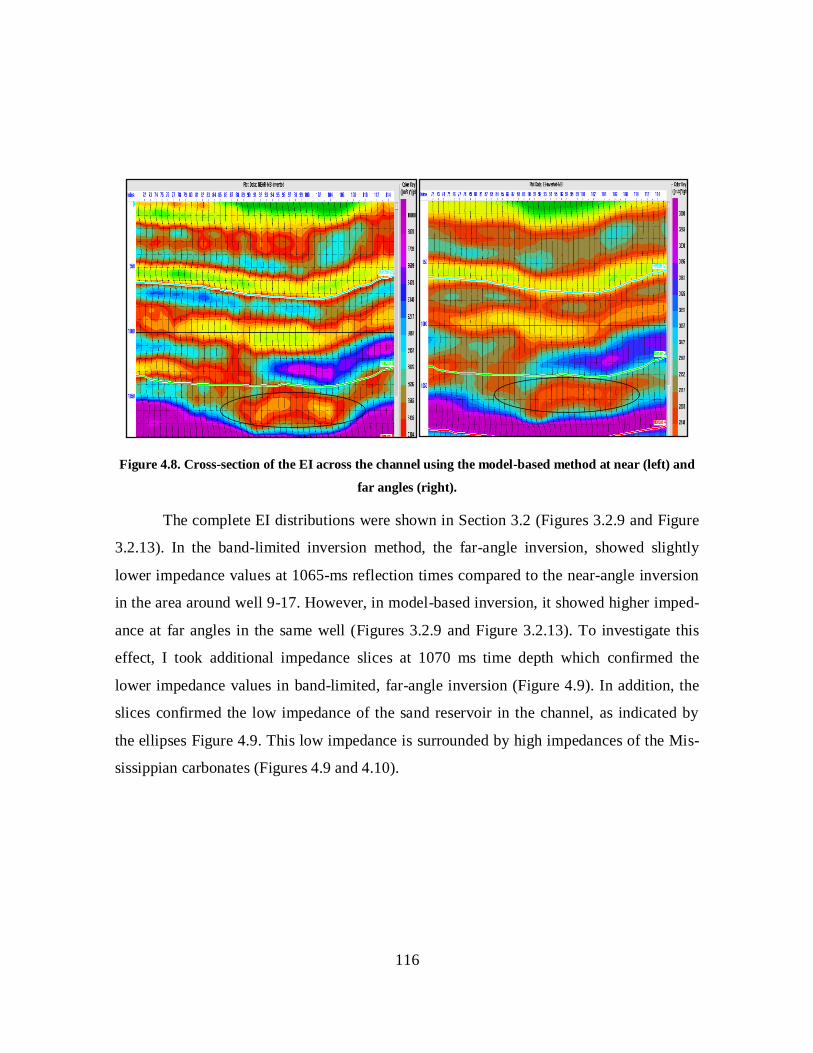
116
Figure 4.8. Cross-section of the EI across the channel using the model-based method at near (left) and
far angles (right).
The complete EI distributions were shown in Section 3.2 (Figures 3.2.9 and Figure
3.2.13). In the band-limited inversion method, the far-angle inversion, showed slightly
lower impedance values at 1065-ms reflection times compared to the near-angle inversion
in the area around well 9-17. However, in model-based inversion, it showed higher imped-
ance at far angles in the same well (Figures 3.2.9 and Figure 3.2.13). To investigate this
effect, I took additional impedance slices at 1070 ms time depth which confirmed the
lower impedance values in band-limited, far-angle inversion (Figure 4.9). In addition, the
slices confirmed the low impedance of the sand reservoir in the channel, as indicated by
the ellipses Figure 4.9. This low impedance is surrounded by high impedances of the Mis-
sissippian carbonates (Figures 4.9 and 4.10).

117
Figure 4.9. Near-offset (left) and far-offset (right) Elastic Impedance slice at 1070 ms time depth using
the band-limited inversion. The low-impedance areas in the channel are indicated by ellipses.

118
Figure 4.10. Elastic impedance slice at 1070 ms time depth using mode-based, near (left) and far
(right). The low-impedance zones in the channel are seen clearly (ellipses).
In the Simultaneous Inversion, we inverted for ZP and ZS and ignored the density
variations (judging them unrecoverable as a result of the narrow angular coverage of CMP
gathers). The RMS data errors (Figure 3.3.4) are lower compared to those of the post-stack
inversion. However, a comparison of the inversion results to the real logs is not quite satis-
factory. The reasons for this is likely that our CMP gathers have comparatively low resolu-
tion which does not allow capturing the details of such a thin reservoir clearly, as well as to
measure the coefficients that are used for background relationship (eqs. 2.4.3 and 2.4.4)

119
more accurately. Nevertheless, the method still shows a good result for ZP and ZS, espe-
cially at the gas well 1-17, as shown in Figure 3.3.5.
Cross-sections zoomed in around the gas well are shown in Figure 4.11. Note the
difference between the P- and S-impedance sections in this Figure. The S-wave impedance
shows relatively high impedance compared to the P-wave impedance, because the shear
wave velocity slightly increases within a hydrocarbon reservoir, unlike the compressional
wave, whose velocity decreases dramatically within a gas reservoir (Gassmann, 1951).
Figure 4.11. P-impedance (top) and S-impedance (bottom) near the gas reservoir. Ellipses indicate the
zone of low P-impedances related to the gas reservoir (above) and relatively high S-impedance (bot-
tom).

120
The RMS impedance distributions averaged within 10-ms time windows centred at
1065 ms (Figure 3.3.7) showed that the simultaneous inversion resulted in higher P-
impedance (ZP) values compared to those derived from post-stack AI inversion (Section
3.1) in the channel area. The S-impedance is quite high within the channel, except around
the gas well 1-17. An additional impedance slice was also taken at 1070-ms time-depth
(Figure 4.12) to illustrate these differences.
Summarizing the AI and EI results, pre-stack inversion (EI) results appear not as
satisfactory as those of the post-stack (AI) inversion. Several reasons may have caused this
deficiency. First, narrow angular apertures (relatively deep reservoir and short source-
receiver offsets) and seismic data quality (such as the limited bandwidth) limit the data
resolution of any inversion. Second, as this study showed, inversion results depend on the
types of algorithms and initial models used. The most high-resolution and model-
independent post-stack algorithm (SILC) is still not available for pre-stack data. Therefore,
it is likely that with its extension to pre-stack inversion and EI, this situation may change.
Third, only standard seismic processing was employed in this study, and potentially there
may exist ways to improve the data quality and to produce higher resolution. For example,
the residual surface-consistent static correction in ProMAX gave unsatisfactory results and
was excluded from the processing sequence. Paucity of well-log data may be another rea-
son, especially of the S-wave logs, which were utilized to calculate the inversion coeffi-
cients .k, kc, m and mc. There are only two S-wave logs within the study area, and both with
limited depth ranges. This could lead to inaccurate inversion coefficients, and consequently
insufficiently inaccurate results. Pre-stack inversion is also stronger affected by the errors
in NMO velocities and by the presence of intra-bed multiples and P/S wave mode conver-
sions.

121
Figure 4.12. P-impedance (left) and S-impedance (right) slices at 1070 ms time depth. The ellipse indi-
cates the channel. The low P-impedance and relatively high S-impedance are visible in the channel.
Further, let us consider the LMR and the VP/VS ratio attributes extracted from
the P- and S-impedances obtained by the simultaneous inversion. As mentioned in the end
of Section 2.1, theoretically, the ρ attribute should be sensitive to pore fluids, whereas ρ
is sensitive to the rock matrix. Specifically, we expect to see lower values of λρ and higher
values of μρ within the gas reservoir (Figure 3.4.1 and 3.4.2). Therefore, the sections were
zoomed in to show the λρ and μρ in the vicinity of the gas reservoir (Figure 4.13). Note the
low λρ and high μρ anomalies indicated by the ellipses in the Figure. The corresponding
VP/VS ratio section is shown in Figure 4.14. As expected, VP/VS decrease significantly

122
within these anomalies. The gas-reservoir anomalies are clearly indicated at 1060-ms re-
flection time.
Figure 4.13. (top) and (bottom) attributes near the reservoir. Ellipses indicate the gas reservoir.
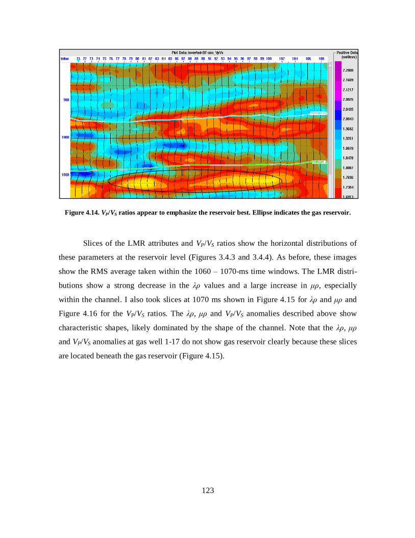
123
Figure 4.14. VP/VS ratios appear to emphasize the reservoir best. Ellipse indicates the gas reservoir.
Slices of the LMR attributes and VP/VS ratios show the horizontal distributions of
these parameters at the reservoir level (Figures 3.4.3 and 3.4.4). As before, these images
show the RMS average taken within the 1060 – 1070-ms time windows. The LMR distri-
butions show a strong decrease in the λρ values and a large increase in μρ, especially
within the channel. I also took slices at 1070 ms shown in Figure 4.15 for λρ and μρ and
Figure 4.16 for the VP/VS ratios. The λρ, μρ and VP/VS anomalies described above show
characteristic shapes, likely dominated by the shape of the channel. Note that the λρ, μρ
and VP/VS anomalies at gas well 1-17 do not show gas reservoir clearly because these slices
are located beneath the gas reservoir (Figure 4.15).

124
Figure 4.15. Slices of LMR parameters 1070-ms time-depth: (left) and (right). The ellipses indi-
cate the channel area. The low- and high- anomalies are shown clearly within the channel.

125
Figure 4.16. VP/VS ratio distribution at 1070-ms time-depth. Note the low VP/VS ratio within the chan-
nel.
Finally, pre-stack CMP gathers were also utilized to create the AVO attribute vol-
umes from the seismic data. Here, the complete intercept (A) and gradient (B) cross-
sections are shown in Figure 3.5.2. The section is also zoomed-in onto the reservoir (Fig-
ure 4.17). The AVO intercept shows a reasonable result in the section containing the gas
well 1-17; however, the gradient seems clearer in showing the top and bottom of the gas in
the section. This could be due to the gradient depending on the changes in density, P-wave
velocity and S-wave velocity with offset (angle) while intercept (A) controlled by the

126
changes in density, P-wave velocity at zero offsets. P-wave velocities decrease dramati-
cally in the case of sand gas whereas S-wave velocity increases only slightly, leading to
increased B values.
Several combinations of A and B are also commonly accepted as AVO attributes
(Section 2.1). A snapshot of the AVO product (AB) taken in the same section confirmed
the gas reservoir very closely (Figure 4.18). When both A and B have large values the
AVO product shows a large positive response at the top and base of the reservoir as indi-
cated in this Figure. The AVO sum (A+B), which is approximately proportional to the
Poisson‟s ratio (Section 2.1) shows a negative response at the top of the reservoir (decrease
in σ) and a positive response at the base (increase in σ) (Figure 4.19). The third AVO at-
tribute is the AVO difference (A-B), which is related to the shear impedance (ZS). This at-
tribute increases at the top of the reservoir (Figure 4.20). The last extracted attribute is
fluid factor (FF), which is related to the deviation from Castagna‟s wet trend equation at
the top and bottom of the reservoir (Section 2.1). The FF is shown in Figure 3.5.10, which
is also zoomed in on the reservoir in Figure 4.21. As expected, there appears to be a rea-
sonable deviation of the FF from Castagna‟s wet trend within the gas reservoir.
In summary, AVO attribute volumes produce reasonable results for the gas reser-
voir, particularly in the area near the gas well 1-17. However, the results of pre-stack at-
tribute inversions largely depend on the density and apertures of the CMP gathers data,
presence of multiples and overall resolution of the seismic data. Unfortunately, it appears
that with the present seismic dataset, this data quality was not sufficient enough to give us
reliable AVO results for the whole area, and our results are focused on the centre where the
angular coverage is the best.

127
Figure 4.17. The AVO intercept A (top) and gradient B (bottom) sections indicate the gas reservoir.
Note that the gradient appears to show a better result (more localized horizontally) than the intercept.
Top of the gas
reservoir
Bottom of the
gas reservoir

128
Figure 4.18. AVO product (AB) indicates the top and the base of the reservoir.
Figure 4.19. Poisson’s ratio at the top and base of the gas reservoir.
Top gas
Bottom gas
Top gas
Bottom gas

129
Figure 4.20. S-wave reflectivity (A-B) indicates the top and bottom of the reservoir.
Figure 4.121. Fluid factor (FF) indicates the deviation from Castagna’s equation at top and bottom of
the reservoir.
Top gas
Top gas Bottom gas
Bottom gas

130
Figure 4.22 show the interpretation of the channel according to a CREWES report
(Lawton, 1995). The channel encounters good sand in the south area around well #8-8. In
this area, the sand is thicker (around 35 meters) while in the north the plugged shale is
encountered in the channel, and the sand is thinner. The images from post-stack inversions
(Figures 4.3 and 4.4) show improved results compared to CREWES interpretation (Figure
4.22). The channel in Figures 4.3 and 4.4 shows low impedance values corresponding to
the thick hydrocarbon sand in the south area. The impedance in northern part of the study
area is higher, likely as a result of plugged shale with sand.
Comparing the performance of the different techniques studied in this Thesis, the
Elastic Impedance corroborated most of the results of post-stack inversion: with the
southern part of the area showing low impedances while the impedances in the northern
part being higher. Simultaneous inversion results were comparatively unsatisfactory in this
study, except at the center of the area where the gas reservoir is located. AVO attribute
inversion was also satisfactory only at the center of the study area with the best angular
coverage and highest CMP fold. However, the VP/VS image derived from simultaneous
inversion showed clear indication of the gas reservoir in the middle of the study area.
Finally, based on the above interpretations, I considered a question where a
hypothetical new well for gas could be drilled in the study area. According the combined
post-stack inversion results corroborated by the pre-stack inversions, the best place for a
potential gas find would be at the center of low-impedance area south of well # 16-8
(Figures 4.3 and 4.4). In this area, most of the methods studies in this Thesis show low
impedance indicating high porosity, and the sand is thicker.

131
Figure 4. 22. Valley of the Blackfoot area extracted from well information (Lawton, 1995).
4.1 Conclusions
This study used the Blackfoot 3D seismic dataset for comparative analysis of sev-
eral types of AVO attributes and inversions. The seismic data were processed by using
ProMAX seismic processing software. Pre-stack and stacked data were further utilized to
perform several types of inversions and to extract a variety of AVO attributes. The final
stacked sections showed good images within the time-depth ranges of 1000 to 1200 ms,
where the target Glauconitic channel is located.
Post-stack inversion was studied by using four methods, three of which utilized the
popular Hampson-Russell (H-R) software, and the fourth (SILC) was included in our in-

132
house package. The results showed that model-based, band-limited and coloured H-R in-
version methods give good and mutually consistent results, with low-impedance zones cor-
responding to the target hydrocarbon sand within the channel. SILC inversion also re-
vealed a low-impedance zone related to the sand in the channel, and demonstrated higher
resolution and improved layer consistency. At the same time, SILC inversion resulted in
somewhat lower background impedances and suggested that merging the seismic and
background models may lead to over-estimated impedances in H-R inversions. Because of
this lower average impedance, colour ranges in plotting the SILC images had to be ad-
justed in order to reveal the details of the reservoir. SILC inversion also better correlated
with the RMS amplitude time slices of the original reflection data. In addition, spatial in-
terpolation was performed differently by the H-R and SILC methods, leading to significant
differences in reservoir details.
In the Elastic Impedance (EI) inversion, the near-angle inversion results were simi-
lar to those of the post-stack inversion (AI). However, the resulting EI values were slightly
lower than I expected from published EI interpretations. The far-angle inversion result also
showed similar results and did not produce the strong EI anomaly, which was also unex-
pected. This relative failure of EI was explained by the insufficient angular aperture of the
seismic data.
Pre-stack inversion was also applied to the CMP gathers to construct the compres-
sional- and shear-wave impedances (ZP and ZS). LMR (, ) attributes and VP/VS ratios
were subsequently extracted from these impedances. The inversion within the gas channel
showed that ZP was higher than the post-stack AI, even though the inversion still gave
good results near the gas well # 1-17 located near the center of the study area and reason-
able values at other locations within the channel. LMR results also showed good results
near the same well.
AVO attributes were also extracted from the processed CMP gathers. Some of
these attributes also allowed a good discrimination of the reservoir near well # 1-17. In par-
ticular, the AVO product (AB), Poisson‟s ratio (A+B) and fluid factor (FF) attributes were
effective in delineating the top and bottom of the gas in this area. The other attributes also
showed reasonable behaviours in the same section. However, generally, it appears that the
AVO attributes suffered from the same limitations as the pre-stack EI inversion, and they

133
were successful only in the center of the study area where the angular coverage was the
best.
In an overall conclusion, post-stack inversion produced the best results suitable for
provisional “targeting” a gas well. Since this method confirm reservoir in the channel area
clearly and comparable to the CREWES result (Lawton, 1995). Pre-stack methods suffer
from the limited quality of the seismic data as well as from paucity of well-log data. The
new SILC method showed good, high-resolution, yet unfortunately distinctly different re-
sults in comparison to the other post-stack methods. It appears that this approach needs to
be further substantiated in other applications and may be very promising in extending to
pre-stack inversion.
4.2 Suggestions for future research
Several ways for extending this study and particularly for improving the pre-stack
results can be suggested. First, the SILC approach (Morozov and Ma, in press) can be ex-
tended to pre-stack analysis. In combination with other advanced current studies of the im-
pedance such as the exact “Zoeppritz” Elastic Impedance and the full P/S impedance
(Morozov, in press), this method could offer great improvements in pre-stack inversion. As
this approach is robust, almost entirely data-driven, and provides high-resolution images, it
holds good promise for improved pre-stack attribute analysis.
As illustrated by the results of this study, the methodology of seismic inversion and
attribute interpretation still needs additional investigations and improvement. My compari-
son of the three popular post-stack inversion schemes to SILC suggested that although
generally mutually consistent, they differ in some important detail of the images. In addi-
tion, they differ significantly from SILC, which is much less dependent on algorithmic nu-
ances. These differences increase away from the wells, showing that spatial interpolation
also has a significant impact on the impedance solutions. This suggests that initial models
and algorithms still determine much of the inverted images, and methods need to be sought
for making the inverse models less dependent on the subjective parameters of the algo-
rithms. Once again, one possible approach to this appears to be SILC (Morozov and Ma, in
press).

134
By using new methodologies, principally new AVO impedance attributes can also
be derived. For example, (Morozov, in press) recently proposed a new definition of the ex-
act P/S impedance which represents a true medium property. This impedance is of a matrix
form and incorporates the P- and S-wave reflections and mode conversions. It is also accu-
rate and does not rely on the traditional approximations to the Zoeppritz equations and
summations of reflectivity series. This accurate form of impedance should be particularly
advantageous with 3C data.
Another significant enhancement could be achieved with Blackfoot 3D-3C data
would be by using the horizontal-component records. In the present study, only the verti-
cal-component data were used in combination with a fairly conventional seismic process-
ing sequence. Full 3C processing requires rotation of the horizontal components, 3C sur-
face-consistent deconvolution and amplitude calibration, and removal of the near-surface
reflection and P/SV conversion effects. Such operations are difficult with the conventional
software, such as Halliburton ProMAX used in this study. Progress in the direction of con-
sistent 3D-3C seismic processing and inversion is also being made in our group (e.g.,
Morozov and Gao, 2009), and such analysis should become feasible in the near future.
Improved seismic waveform processing to increase its resolution could also help
imaging the thin Blackfoot reservoir. A more accurate determination of the seismic wave-
let should lead to improved resolution of the inversion and all attributes. Also, a more pre-
cise suppression of multiples and mode conversions (compared to the present NMO cor-
rection and CMP stacking) could improve the correspondence of the wavefield to the con-
volutional model used in inversion.

135
REFERENCES
Aki, K., and Richards, P., 2002. Quantitative seismology: theory and methods,, Second
Edition, University Science Books, Sausalito, CA.
Connolly, P., 1999. Elastic impedance. The Leading Edge, 18, 438-452.
Castagna, J. P., Batzle, M. L., and Eastwood, R, L., 1985. Relationships between compres-
sional-wave and shear-wave velocities in clastic silicate rocks Geophysics, 50, 571-
581.
Castagna, P. J., and Smith, S. W., 1994. Comparison of AVO indicators: A modeling
study. Geophysics, 59, 1849-1855.
Castagna, J. P., Swanz, H. W., and Foster, D. J., 1998. Framework for AVO gradient and
intercept interpretation. Geophysics, 63, 948-956.
Fatti, J. L., Smith, G. C., Vail, P. J., Strauss, P. J., and Levitt, P. R., 1994. Detection of gas
in sandstone reservoirs using AVO analysis: A 3-D seismic case history using the
Geostack technique. Geophysics, 59, 1362-1376.
Gassmann, F., 1951. Elastic waves through a packing of spheres: Geophysics, 16, 673-685.
Gardner, G. H. F., Gardner, L.W., and Gregory, A. R., 1974. Formation velocity and densi-
ty - The diagnostic basics for stratigraphic traps, Geophysics, 39, 770-780.
Goodway, B., Chen, T. and Downton, J., 1997. Improved AVO fluid detection and litholo-
gy discrimination using Lamé petrophysical parameters; ``lambda rho'',``mu
rho'',&``lambda/mu fluid stack'', from P and S inversions, SEG Expanded Abstracts
16, 183-186.
Gulati, J. S., Stewart, R. R., Peron, J., and Parkin, J. M., 1997. 3C-3D VSP: Normal mo-
veout correction and VSPCDP transformation. CREWES Research Report- 9
Lawton, D. C., 1996. Design review of the Blackfoot 3C-3D seismic program. CREWES
Research Report –38.
Lawton, D.C., Stewart, R. R., Cordsen, A and Hrycak, S, 1995. Advances in 3C-3D design
for converted waves. CREWES Research Report –43.

136
Larsen, J. A., Margrave. G. F., Lu, H., and Potter, C. C., 1998. Simultaneous P-P and P-S
inversion by weighted stacking applied to the Blackfoot 3C-3D survey. CREWES
Research Report – 50
Lindseth, R. O., 1979. Synthetics sonic logs- a process for stratigraphic interpretation:
Geophysics, 44, 3-26.
Lancaster, S., Whitcombe, D., 2000. Fast-track „coloured‟ inversion. SEG Expanded Ab-
stracts, 19, 1572-1575.
Ma, J., 2003. Forward modeling and inversion methods based on generalized elastic im-
pedance in seismic exploration. Journal of Chinese Geophysics, 46,159-168.
Margrave, G. F., Lawton, D. C., Stewart, R. R.. 1998. Interpreting channel sands with 3C-
3D seismic data. The Leading Edge, 17,509-513.
Martins, J. L., 2006. Elastic impedance in weakly anisotropic media, Geophysics, 71, D73-
D83.
Morozov, I. B., and Ma, J. in press, Accurate post-stack acoustic impedance inversion by
well-log calibration, Geophysics, in press.
Morozov, I. B., and Gao, L., 2009. Pre-stack calibration of 3-C 3-D time-lapse seismic da-
ta, 2009 CSPG/CSEG/CWLS Convention, May 4-6, 2009, Calgary, AB.
Morozov, I. B., Exact Elastic P/SV impedance, Geophysics, in press..
Miller, S. L. M., Aydemir, E. O., and Margrave, G. F., 1995. Preliminary interpretation of
P-P and P-S seismic data from the Blackfoot broad-band survey. CREWES Re-
search Report-42.
Ostrander, W. J., 1982. Plane wave reflection coefficients for gas sands at non-normal an-
gles of incidence: SEG Expanded Abstracts, 1, 216-218.
Pendrel, J, 2006, Seismic inversion- Still the best tool for reservoir characterization,
CSEG, Recorder, 5-12.
Rutherford, S. R., and Williams, R. H., 1989, Amplitude-versus-offset variations in gas
sands: Geophysics, 54, 680–688.
Russell, B., and Hampson, D., 1991. Comparison of Poststack Seismic Inversion Methods,
SEG Expanded Abstracts,10, 876-878.

137
Russell, B., 1988, Introduction to seismic inversion methods: The SEG course notes Series,
2.
Santos, L. T. and Tygel, M., 2004. Impedance-type approximations of the P–P elastic ref-
lection coefficient: Modeling and AVO inversion. Geophysics, 69, 592-598.
Sheriff, R.E., and Geldart, L. P, 1995. Exploration Seismology. Cambridge ; New York :
Cambridge University Press, 1995, 592.
Shuey, R.T., 1985, A simplification of the Zoeppritz equations: Geophysics, 50, 609-614.
Smith, G. C., and Gidlow, P. M., 1987. Weighted stacking for rock property estimation and
detection of gas: Geophysical Prospecting, 35, 993-1014.
Simin, V., Harrison, M. P., and Lorentz, G. A., 1996. Processing the Blackfoot 3C-3D
seismic survey. CREWES Research Report-39.
Simin, V., Margrave, G. F., and Yang, G. Y.C., 1996. AVO measurements for P-P and P-
S data in the Blackfoot 3C-3D dataset. CREWES Research Report-42.
Singh, Y., 2007, Lithofacies detection through simultaneous inversion and principal com-
ponent attributes. The Leading Edge, 26,1568-1575.
Stewart, R. R., Gaiser, J. E., Brown, R. J., and Lawton, D. C., 1999. Converted-wave seis-
mic exploration: a tutorial. CREWES Research Report -3.
VerWest, B., 2004, Elastic Impedance revisited, 66th EAGE Conference and Exhibition
Extended Abstracts, Paris, France, P342.
VerWest, B., Masters, R., and Sena, A., 2000. Elastic impedance inversion: 70th Ann. In-
tern. Mtg. Soc. Expl. Geophys. Expanded Abstracts, 1580-1582.
Whitcombe, D. N. 2002. Elastic impedance normalization, Geophysics, 67, 60-62.
Whitcombe, D. N., Connoly, P., Reagan, P. L., and Redshaw, T. C., 2002. Extended elastic
impedance for fluid and lithology prediction, Geophysics, 67, 63-67.
Wiggins, R., Kenny, G.S., and McClure, C.D., 1983. A method for determining and dis-
playing the shear-velocity reflectivities of a geologic formation: European patent
Application 0113944.
Xu, Y and Bancroft, J. C., 1997. Joint AVO analysis of PP and PS seismic data CREWES
Research Report -34.

138
Yalmaz, O., 2006. Seismic data analysis: processing, Inversion and Interpretation of seis-
mic data: Society of exploration geophysics. 1793-1999.
Zhang. Q., Stewart, R. R., Parkin, J. M., and Sun. Z., 1996. Analysis of the Blackfoot 3C-
3D VSP survey. CREWES Research Report-40.


![OPTICAL CHARACTERIZATION OF RARE EARTH …ecommons.usask.ca/bitstream/handle/10388/etd-07292009-064945/Go... · ... Dr. S. O. Kasap, ... Photon Amplification [13] ... Er3+ ion energy](https://static.fdocuments.us/doc/165x107/5abdc1f17f8b9aa3088c06d3/optical-characterization-of-rare-earth-dr-s-o-kasap-photon-amplification.jpg)


