Positive Spillovers and Free Riding in Advertising of Prescription

Pharmaceuticals: The Case of Antidepressants

Bradley T. Shapiro∗

This Version May 19, 2015

Abstract

Television advertising of prescription drugs is controversial, and it remains illegal in all but two countries. Much

of the opposition stems from concerns that advertising directly to consumers may inefficiently distort prescribing

patterns toward the advertised product. Despite the controversy surrounding the practice, its effects are not well

understood. Exploiting a discontinuity in advertising along the borders of television markets, I estimate that television

advertising of prescription antidepressants exhibits significant positive spillovers on rivals’ demand. I then construct

and estimate a multi-stage demand model that allows advertising to be pure category expansion, pure business stealing

or some of each. Estimated parameters indicate that advertising has strong market level demand effects that tend to

dominate business stealing effects. Spillovers are both large and persistent. Consistent with these spillovers, I find

that firms advertise less and are less likely to advertise in markets with positive shocks to rival advertising. Using

the demand estimates and a stylized supply model, I explore the consequences of the positive spillovers on firm

advertising choice. Compared with a competitive benchmark, simulations suggest that a category-wide co-operative

advertising scenario would produce four times as much advertising, resulting in a 18 percent increase in category size

and a 14 percent increase in category profits.

1 Introduction

How does television advertising affect the consumer choice problem? After a consumer watches a commercial, in-ternalizes its message and decides a product is desirable, she must take further action to obtain the product. Withgroceries, she must go to the supermarket. With many consumer products, a computer with internet will allow theconsumer to make the purchase. With prescription drugs, the consumer must go to the physician to obtain a prescrip-tion and then to the pharmacy to purchase the drug. With many steps between the advertising incidence and purchase,at some stage of the process, the consumer might well choose a different product from the one advertised. This may be∗University of Chicago Booth School of Business. I thank Nancy Rose, Ernst Berndt, and Stephen Ryan for all of their advice. I would also like to extend my

gratitude to Andrew Ching, Sara Fisher Ellison, Glenn Ellison, Günter Hitsch, Greg Leiserson, Sarah Moshary, Jesse Shapiro, Xiao Yu May Wang, and two anonymousreferees for their helpful suggestions. This paper also benefited from conversations with Paul Snyderman and Len Tacconi; as well as participants at the MIT IndustrialOrganization seminar and field lunch. I thank Cindy Halas at IMS Health, Jackie Allen and Leslie Walker at Kantar Media Intelligence, and LuAnn Patrick and PatrickAngelastro at ImpactRx for their help with data resources. This research was supported by the National Institute on Aging, Grant Number T32-AG000186 and theNational Science Foundation Graduate Research Fellowship under Grant Number 1122374. All mistakes are my own.

1

due to difficulty in remembering advertisements, agency problems in obtaining products or simply because advertisingconvinces a consumer to go to a retailer, computer or physician. In short, an advertisement could affect the choiceprocess without leading the consumer to buy the advertised product.

In this paper, I identify the existence of positive spillovers of television advertising in the market for antidepressants.Given this, I construct and estimate a demand model which allows such spillovers. Given these spillovers, I test to seeif firms free ride off of rivals’ advertising. To quantify the potential size of the incentive effects of spillovers on firmbehavior, I conduct a supply side analysis supposing that the firms are able to jointly decide advertising, and I comparethis outcome to a benchmark competitive outcome in the antidepressant market.

Branded television advertising of prescription drugs is contentious and has been condemned by many as inefficientlydistorting prescriptions to the advertised products. In fact, it is legal in only two countries: New Zealand and the UnitedStates. In light of the controversy, it is important to understand the impact of these advertisements. In particular,understanding spillovers is crucial to regulators, firms and econometricians. From a regulatory perspective, the Foodand Drug Administration (FDA) regulates the content of advertisements. To the extent that advertising content is mademore informative and less brand specific, content regulation could exacerbate spillovers. Firms may lose individualincentives to advertise as spillovers intensify. This could be either good or bad for social welfare depending on whetheror not category expansion is a public good or a public bad. However, it is an important consideration for the regulatorin either case. From a firm strategy perspective, understanding possible channels for revenue improvement is vital.While cooperation is often difficult to enforce and non-contractible due to antitrust laws, advertising cooperatives areprecedented in other industries such as orange juice, milk and beef. Finally, from a technical perspective, failureto model spillovers in advertising can distort estimated parameters, leading to incorrect inferences about supply anddemand.

Previous research incorporating advertising into demand analysis has frequently treated advertising of a product asaffecting its probability of being in the choice set (Goeree 2008) or has incorporated advertising into a productionof goodwill that enters directly into the utility function (Dube et. al. 2005). However, such specifications alsotypically exclude the possibility of positive spillovers of advertising onto rivals. While this eliminates the complexityof modeling behavior in the presence of possible free riding, such an exclusion may lead the researcher to missimportant strategic considerations. When deciding how much to advertise, firms do not internalize the benefit theyprovide to other firms and have an incentive to free ride on their rivals’ advertising efforts. Understanding theseconsiderations is important for marketing decision makers as well as policy makers potentially seeking to regulateadvertising.

Prescription drugs in general, and antidepressants in particular, have many characteristics which facilitate positivespillovers in television advertising. First, the FDA regulates what firms can and cannot say in advertisements. Whilethe name of the product is typically prominently displayed throughout the commercial, most of the time in eachcommercial is spent explaining the ailment, the mechanism of action of the drug and its side effects. When thereare several therapeutic products available, those treating the same ailments tend to share common characteristics. Aconsumer might remember all of the things being said but forget the name of the product. Agency problems furtherdisrupt this link. A consumer must see a doctor to get a prescription. A physician might have different preferences oropinions about which drugs, if any, work best for a given condition or patient. The advertisement may lead a patientto the physician, but the physician remains the ultimate arbiter of whether and what to prescribe.

My strategy for evaluating the extent of positive spillovers in advertising for antidepressants proceeds in three steps.First, I use discrete television market borders to determine the extent to which advertising does affect rival demand,

2

positively or negatively. Next, I construct and estimate a model of the antidepressant market, allowing advertisingto have positive spillovers on demand of horizontally differentiated products, a feature excluded by typical discretechoice specifications. Positive spillovers are allowed, but not imposed by the model. Further, I find that not using theborder discontinuity and assuming advertising choices are exogenous leads the researcher to over-state the long runeffectiveness of advertising as well as understate the extent of the positive spillover. Next, I test whether firms freeride off of rival advertising efforts. I find that firms advertise less and less often when there are positive shocks torival advertising in a given market. Finally, given estimates of the demand effects and an assumed marginal cost ofadvertising, I quantify the importance of free riding by simulating a stylized supply model and compare a benchmarkcompetitive outcome with a scenario whereby a co-operative sets advertising for the entire industry.

While most models incorporating advertising into demand have not allowed for positive spillovers, there are studiesof Direct-to-Consumer (DTC) advertising in pharmaceuticals with varying credibility of identification strategies thathave shown some evidence that cross advertising elasticities could be positive, but results have been mixed. In contrastto the demand analyses mentioned above that typically do not allow for cross advertising elasticities to be positive,these studies tend to find patterns that are consistent with spillovers, rather than allowing for spillovers within ademand model. In particular, [Iizuka & Jin (2005), Berndt et. al. (2004), Wosinska (2002)], find very small estimatesof advertising effects on market shares conditional on being in the market and conclude that it might be exhibitingpositive spillovers, though spillovers are neither directly modeled nor tested. Wosinska (2005) and Donohue et. al.(2004) find that advertising has positive spillover effects onto drug compliance and duration of treatment. Other studiesfind that advertising drives consumers to the doctor (Iizuka & Jin 2004) or has class level effects (Rosenthal et. al.2003, Avery et. al. 2012), but they do not model any product level own or cross-elasticities of advertising. Berndt et.al. (1995, 1997) estimate the effect of marketing on both the size of the market and on brand shares, focusing mostlyon physician detail advertising and academic journal advertising since DTC was extremely limited and unbrandedat the time, and found some effects at both category and product levels. In studying detailing effects, Ching et. al.(2012) take advantage of the fact that identical molecules are sometimes marketed by different firms under differentnames in Canada to separate out brand versus category effects. Narayanan et. al. (2004) estimate a two level modelusing only time series variation for antihistamines and do not find positive spillovers. In experimental work, Kravitzet. al. (2005) find mixed results for patients going to their physicians asking for products they saw on television. Ina structural model, Jayawardhana (2013) imposes that television advertising must only affect class level demand andfinds significant effects. Many of these studies either only model a category level response or only model a conditionalshare level response. This paper will model the full decision process and use data with both spatial and time seriesvariation. Stremersch et. al. (2013) and Liu & Gupta (2011) also examine the various effects of DTC on aspects ofdemand1. Stremersch et. al. can explain variation across geography using demographic characteristics and both findheterogeneous effects. This study will differ from both of those in that fixed effects will be used to partial out thereasons for persistent differences in DTC across markets and focus on variation just across the borders.

The supply side of advertising in pharmaceuticals has been much less explored. If advertising helps rivals’ demand,there might well be an incentive to invest less in advertising. Iizuka (2004) finds that as the number of competitorsincreases, firms advertise less, leading him to suggest the existence of a free riding problem. Ellison and Ellison (2011)find evidence that pharmaceutical firms decrease advertising just prior to patent expiration in order to make the marketsmaller and deter generics from entering. The possibility of such strategic deterrence implies the existence of positivespillovers, at least from brand to generic. However, no research that I am aware of uses a supply model to quantify

1Stremersch et. al. (2013) looks at the effects of DTC through the mediator of patient requests and finds no effects. Liu & Gupta (2011) useinformation on patient visits.

3

the magnitude of the potential positive spillover effects on advertising expenditure decisions. Ching (2010), Filson(2012), Liu et. al. (2013) all use a Markov Perfect Equilibrium concept to model the supply side of pharmaceuticalmarkets, but they all focus on different aspects of the pharmaceutical industry rather than television advertising.

Outside of the pharmaceutical literature, Sahni (2013) finds experimental evidence of positive spillovers to rivalsin online restaurant advertising in India. Additionally, Lewis & Nguyen (2012) and Anderson & Simester (2013)find evidence of positive spillovers in a number of categories for online and mail advertising, respectively. Non-experimentally, Ching et. al. (2009) show evidence from scanner data that advertising of an individual brand with adisplay or feature could have spillover effects for the whole category.

The contributions of this paper are threefold. First, I improve upon the literature that seeks to identify the causal effectof advertising on own and rivals’ demand with observational data by using an identification at the border approach.That is, I will identify advertising elasticities by comparing households that are very near to each other geographicallybut get different advertisements due to the way the television market borders are drawn. I show that advertising hassignificant positive effects on rivals’ sales, though smaller than its effects on own firm sales. I construct and estimatea consumer choice model, which allows advertising to influence the size of the category, the conditional share of eachsubcategory in the category, and the conditional share of each product in a subcategory. I will consider the category,the subcategory and the product levels as three separate stages of a joint physician-consumer decision making process.At each stage, I will allow for advertising carry-over effects. Results indicate that advertising of antidepressants affectsboth category demand and brand share. The category effects are larger and more persistent over time than are businessstealing effects, leading to a net positive spillover. Further, using the border strategy with fixed effects to identifythe advertising parameters is important. Failing to use fixed effects to control for persistent differences in marketsand systematic national changes over time in market conditions leads the researcher to conclude that advertising isprimarily business stealing and drastically over-states the short and long run effectiveness. Failing to focus on theborders of television markets to control for the endogeneity of firm choices leads the researcher to over-state the longrun effectiveness of advertising and under-state the relative long run importance of category expansion relative tobusiness stealing. Next, as the estimated demand parameters imply an incentive for firms to free ride, I directly testwhether firms advertise less or less often in markets where rivals have idiosyncratically high advertising. Consistentwith these incentives, I find that firms advertise less and less often in markets where rival advertising is high. Finally,I conduct a supply side analysis using a stylized model to evaluate to what extent positive spillovers suppress theincentive to advertise. Given the demand parameters, I compute a benchmark competitive outcome in televisionadvertising. I find that if instead, firms that advertise work together, removing the need for strategic response, thosefirms would combine to advertise 50% more than in competitive equilibrium. A co-operative deciding all advertisingexpenditure levels taking full industry profits into account would advertise four times as much as is observed incompetitive equilibrium, increase the category size by 18% and category profits by 14%. No other research that I amaware of conducts such a supply side analysis of the provision of advertising that exhibits positive spillovers. Thispaper helps move us toward understanding the effects of advertising and the incentives facing the firms who provideit, and understanding both are essential to firm profit maximization and to efficient regulation.

4

2 Empirical Setting

2.1 Prescription Drugs and Advertising

Television advertising of prescription drugs did not appear in the United States until 1997. While technically notforbidden by law, advertising was required to have much more risk information included on all advertisements than isrequired today. This required risk information was similar to the package inserts that come with prescriptions. Readingthose aloud in the context of a thirty second spot was prohibitively time consuming and costly. In the fall of 1997, theFDA issued a draft memorandum clarifying their stance on advertising risk information, allowing advertisements toair so long as they had a ‘fair balance’ of risk information, even if abbreviated. Firms had the opportunity to submittheir advertisements to the FDA for pre-approval to ensure that the ‘fair balance’ condition was met. In 1999 the finalcopy of the FDA memorandum was circulated. The first advertisements on television for antidepressants were seen in1999 when GlaxoSmithKline’s brand, Paxil, began airing its first campaigns.

Figure 1 suggests that the FDA regulation was binding prior to 1999, and advertising did not begin until that point.

2.1.1 Antidepressants

Prescription antidepressants are indicated for treatment of major depressive disorder and dysthymia, which is a moreminor version of depression. Traditionally, depression was treated with what are called tricylcic antidepressants(TCAs), which were discovered in the 1950s, but those came with significant side effects and risks. Treatment ofdepression took a great leap forward in the late 1980s with the innovation of selective serotonin reuptake inhibitors(SSRIs), the first of which was Prozac. Newer generation antidepressants are more tolerable than the older generationTCAs and allow patients to be more safely treated and with fewer side effects (Anderson 2000). This allows easiermanagement of antidepressant treatment by primary care physicians, and makes seeing a specialist less necessary.

Diagnosis and treatment of depression can be rather complicated, as with many mental disorders. As the class of drugshas grown, so have the number of people being treated. In 1996, the industry pulled in around $5 billion in revenue.By 2004, it was up to $13 billion. In 2004, an FDA black box warning was instituted suggesting that antidepressantsmight lead to an increase in suicidality among adolescents (Busch et. al 2012). Around the same time, many widelyselling molecules began to go off patent. Figure 2 shows the revenues of the antidepressant industry from 1996 through2004. Since the discovery of Prozac, ten other brands, some with slightly different mechanisms, have been discoveredand have entered the market. Some of those have developed extended release versions which allow patients to havefewer doses per day.

There are six main subcategories of antidepressants: the old style TCAs, Tetracylcic (TeCA), Serotonin Antagonistand Reuptake Inhibitors (SARI), Serotonin-norepinephrine Reuptake Inhibitors (SNRI), Norepinephrine ReuptakeInhibitors (NDRI) and SSRI. While the specific differences between these are not important to this study, it is worthnoting that each subcategory has somewhat different mechanisms, interactions and side effect profiles from the others.Deciding which subcategory of antidepressant is appropriate for a given patient is largely up to the physician, and oftenis related to other medications the patient is taking. The decision between drugs within a subcategory might dependon what is included on the patient’s insurance formulary or physician preferences. Antidepressants are characterized

5

by a high degree of experimentation to find a good fit between treatment and patient, as well as a low compliance ratedue to the many side effects (Murphy et. al. 2009).

Many physicians see depression as an under treated condition and some research has concluded that restricting accessto antidepressants has been associated with negative health outcomes (Busch et. al. 2012). Given this information, itis plausible that market expansive advertising could play a role in this market.

2.1.2 The Market for Advertising

Firms can purchase advertising space on television in two ways. First, there is an upfront market each summer whereadvertising agencies and firms make deals for the upcoming year of television. Advertising purchased in the upfrontmarket cannot be “returned” and typically has minimal flexibility in terms of timing. Next, there is a spot market thatis called the ‘scatter’ market, where firms can purchase advertising closer to the date aired.

Additionally, there are both national and local advertisements. National advertisements are seen by everyone in thecountry tuned into a particular station, while local advertisements are only seen by households within a particulardesignated market area (DMA).

A DMA is a collection of counties, typically centered around a major city, and it is defined by AC Nielsen, a globalmarketing research firm. The DMAs were first defined to allow for the sale of advertising in a way that was straight-forward to the advertisers. The DMA location of a county determines which local television stations that a consumerof cable or satellite dish gets with his or her subscription. The original idea was to place counties into the same DMAwith the local television station that most people wanted to watch, which often times was just the station that waseasiest to pick up over the air. That is, if a county picks up the Cleveland stations over the air more easily than theColumbus stations, it would be placed in the Cleveland DMA. Existing laws and regulations in most circumstancesdo not allow satellite or cable operators to provide broadcast signals from outside of the DMA in which they reside.2

Even for over the air signals, the FCC moderates the signals to try to keep the signal from each station localized onlyin its own DMA.3 There are 210 DMAs in the United States, the largest 101 of which are included in my data.4

From informal conversations with individuals in industry, I learned that pharmaceutical companies participate almostexclusively in the up front market. Like most consumer goods, the majority of antidepressant spending is on nationaladvertising, but there is a significant amount of local advertising as well as significant variation across DMAs in theamount of local advertising.

Prices for advertisements typically are determined by projected volume and type of viewership. A single airing ofa national advertisement for antidepressants ranges from $1,600 to $23,000 from 1999-2003 and a single airing of alocal advertisement ranges from $0 to $7,600 for the same time period. Looking at each advertisement in terms ofexpenditure per capita, I observe that the distribution of local advertising expenditure per capita on a single commerciallooks similar to the distribution of national advertising expenditure per capita on a single commercial. National

2http://www.sbca.com/dish-satellite/dma-tv.htm3http://www.fcc.gov/encyclopedia/evolution-cable-television4I note here that from time to time, Nielsen may move one county from one DMA into another. In this data, I have a snapshot of DMA

composition currently. Discussions with Nielsen have assured me that these shifts are sufficiently infrequent and few that using current DMAinformation should not be problematic. To the extent that a county gets categorized in the wrong DMA, it will lead to measurement error that willbias estimates towards zero.

6

advertisements range from $0.0002 per 100 to $0.04 per 100 and 93% of local advertisements fall within that rangeas well, with a few outliers going down to zero and up to $0.20 per 100 capita. By scaling expenditures by potentialviewing population, local and national advertising expenditures are comparable.

Additionally, only four brands from three firms in this market advertise at all. Eli Lilly (Prozac, Prozac Weekly), Pfizer(Zoloft) and GlaxoSmithKline (Paxil, Paxil CR, Wellbutrin SR, Wellbutrin XL) are the only firms advertising in thismarket. Notably, those firms, along with Merck, are some of the largest advertisers among all of the pharmaceuticalindustry (Berndt et. al. 2003). The lack of advertising from all firms could be indicative of fixed costs of advertisingat all or of free riding. Those branded products which do not advertise either have low market share (Effexor XR,Remeron, Serzone) or have a very small parent company which might be less likely to have an advertising division(Celexa, Lexapro). Whether or not we can observe free riding will be further evaluated in the supply analysis.

2.2 Data

2.2.1 Prescribing Data

Sales data for this market comes from the Xponent data set of IMS Health, a health care market research company. Theprescribing behavior of a 5% random sample of physicians who prescribe antidepressants is followed monthly from1997 until 2004. The data include a rich set of physician characteristics including address of the primary practice,which is then linked to county. The data used in this study is aggregated to the county level and ends with 2003,thereby avoiding confounding market changes in 2004 including the FDA black box warnings and wave of patentexpirations. The sample is partially refreshed annually.

2.2.2 Advertising Data

Product level monthly advertising data at the national and Designated Market Area (DMA) level for the top 101 DMAscomes from Kantar Media. In addition to advertising expenditures, the data includes number of commercials. Theunit of advertising used in this study will be expenditures per 100 capita in the viewing area. Scaling expendituresby population in the viewing area allows me to have a comparable measure of advertising volume between nationaland local advertising. Total advertising for a county is defined as the national advertising expenditure scaled by thenational population plus the local advertising expenditure scaled by the population of the DMA.5 Table 1 providesdescriptive statistics for the DMA level advertising variables at the product, subcategory and category level for theperiod of the data where advertising is allowed: September 1999 through December 2003. The statistics are also onlyon the products that ever advertise: Paxil, Paxil CR, Prozac, Prozac Weekly, Wellbutrin SR, Wellbutrin XL and Zoloft.

Figure 3 depicts local advertising expenditures per 100 capita in Boston, New York and Austin as well as national asexamples of what local advertising expenditures look like over time. Local advertising for Paxil is higher in New Yorkthan it is in Boston, which in turn is higher than it is in Austin, suggesting that there is non-trivial variation acrossmarkets in this measure. National advertising makes up the bulk of the advertising that households see, but the localadditions to the national advertising vary a great deal.

5A possible alternative measure would be to use the number of commercials at the national level plus the number of commercials at the locallevel. I explored using that measure and the results were not qualitatively different. However, as a commercial during the evening news is likely tocapture far more eyeballs than a commercial during a 1:00 AM rerun of MacGyver, using expenditures per 100 capita would seem to do a better jobat measuring quality adjusted advertising than number of commercials.

7

2.2.3 Detailing Data

In addition to DTC data, I have collected physician level detailing data from ImpactRx, a market research firm. Inthe data, a panel of 2134 general practice physicians are followed monthly through time from 2001 through the endof 2003, and a panel of 167 psychiatrists are followed monthly for 2002 and 2003. This panel is a national andgeographically representative sample of physicians, most of whom are in the 40th percentile or greater in terms oftotal prescriptions written. This non-representativeness is due to the fact that these are the physicians who are mostlikely to ever be detailed. While these physicians make up less than 1% of total physicians in the country, they arelikely to make up a significantly higher percentage of both the prescription and detailing distributions. Additionally,national aggregate detailing data by brand from IMS Health is observed in the data.

2.2.4 Other Data Sources

I observe prices from Medicaid reimbursement data, collected by the Centers for Medicare & Medicaid Services(CMS). Duggan and Scott-Morton (2006) argue that the average price that Medicaid pays per prescription prior toMedicaid rebates is a good measure of the average price of a drug on the market. As my measure of price, I use thetotal Medicaid units dispensed divided by the total Medicaid reimbursements during a quarter for a particular product,deflated to 2010 dollars using the consumer price index.

CMS also collects data on the average pharmacy acquisition cost for all pharmaceutical products (NADAC). As I willnot be estimating marginal production costs empirically, these average pharmacy acquisition costs may be used as aneffective upper bound on marginal production costs. While there are markups from branded drugs, pharmacies aretypically able to obtain generics at much lower rates, particularly when there are several generic competitors (as is thecase in this market), often as low as ten cents per pill. As of 2013, all products in the sample have generic versionsavailable. For an upper bound on the marginal cost of each drug, I use average pharmacy acquisition cost for thosegeneric version of the product, deflated to 2010 dollars using the consumer price index.

Yearly county population, employment, demographic and income data are drawn from the Current Population Survey(CPS).

3 Reduced Form Evidence

In this section, I explore the data to see if spillover effects exist and how they interact with own effects. This exercisehas been difficult to implement in previous research, largely due to data limitations. Estimates show that rivals’ andown advertising have a positive effect on sales, while rivals’ advertising has a smaller effect than own advertising. Inaddition, the cross partials indicate that rivals’ advertising makes own advertising less effective, but own advertisinghas a larger negative effect on the marginal own advertisement due to decreasing returns to scale.

In particular, I model sales of quantities Q of product j in time t for market m as a function of own advertising, aown,and advertising of rivals, across:

8

log(Q jmt) = λ log(Q jm,t−1)+ γ1aownjmt + γ2across

jmt + γ3(aownjmt )

2 + γ4(acrossjmt )2 + γ5aown

jmt acrossjmt + ε jmt (1)

This provides insight on whether rivals’ advertisements help or hurt own demand, the nature of decreasing returns toscale, and persistence in advertising effects.

3.1 Empirical Identification Strategy - Border Strategy

The endogeneity of advertising and the absence of obvious instruments pose challenges to causal identification of theeffect of advertising on demand.

I address the endogeneity concerns associated with advertising decisions by taking advantage of the discrete natureof local advertising markets. That is, two households which are directly across the television market border from oneanother will see different advertisements despite being otherwise very similar households. I take advantage of thiscomparison. This approach is similar in spirit to that used by Card and Krueger (1994) and Dube et. al. (2012) toidentify the effects of minimum wage increases and that used by Holmes (1998) to identify the effect of right-to-worklaws. These three studies rely on state borders, across which any number of laws, market conditions or preferencesmay vary. Similar spatial strategies have also been used by Black (1999) and Bayer et. al. (2007) using school zoneborders and Ito (2014) using electricity market borders. A nice feature of television market borders is that they wereset with television in mind and have very little correspondence with anything else in the world. As such, we mightthink the location of DMA borders is far more exogenous to consumer characteristics than are state borders.

Advertising is purchased both nationally and locally. The level of total advertising that a household gets to its televisionis determined by the Designated Market Area (DMA) that the household’s county belongs to, as defined by AC Nielsen.Nielsen places counties into markets by predicting which local stations the households will be most interested in. Assuch, DMAs tend to be centered at metropolitan areas. A map of all of the DMAs included in the advertising data ispresented in Figure 4.

To get an idea of how advertising is distributed across the country, consider the example of the Cleveland and ColumbusDMAs. Figure 5 depicts the state of Ohio with each DMA in a different color. Every county in the mustard colorCleveland, Ohio DMA gets the same amount of the same advertising as every other county in the Cleveland DMA.Meanwhile, every county in the green color Columbus, Ohio, DMA gets the same amount of the same advertising asevery other county in the Columbus DMA, though this might be different from the advertising in the Cleveland DMA.Meanwhile, these two DMAs border each other. There are five counties in the Cleveland DMA which share a borderwith at least one county in the Columbus DMA and five counties in the Columbus DMA which share at least oneborder with a county in the Cleveland DMA. My strategy will be to consider these ten counties as an experiment withtwo treatment groups (Cleveland and Columbus) in each time period.

The data contain 153 such borders. The map of all of the counties included in this border sample is presented in Figure6. Each of these borders will be considered a separate experiment, with the magnitude of the treatment determined bythe advertising in each DMA at a given time. Only the counties bordering each other will serve as controls for eachother to partial out any local effects that may be increasing or decreasing for both sides of the border. The level ofan observation is a product-border-DMA-month. This means that a group of counties along a particular border but

9

in the same DMA are aggregated together, as they see they each see the same advertising and they are each beingcompared with a similar group across the border. In each ‘experiment,’ one such set of counties will be compared withan adjacent set of counties across the DMA border. For each border experiment in each time period, there will be twoobservations: one for the group of counties on one side of the border and one for the group of counties on the otherside of the border. Each of these observation groups will constitute a market.

To estimate the effects of advertising in this experiment, I will use a modified difference-in-differences estimator. Theidentifying assumption is that along the border of two DMAs, any differential trends in demand between the two sidesof the DMA border stem from differences in advertising. In particular, I use panel data with fixed effects. Border-timefixed effects will ensure that the common trend assumption is only enforced locally at the border between two DMAs,allowing for spatial heterogeneity. Border-DMA fixed effects will allow systematically different demand levels acrossthe border. I will also include a lagged dependent variable to get at the dynamic effects of advertising. Consider thelog of quantity log(Q jbmt), at the product-border-DMA-month level. Advertising, a jmt , as mentioned before lives atthe product-DMA-month level and affects log(Q jbmt) through some function f :

log(Q jbmt) = f (a jmt)+ ε jbmt

Each product-border pair will constitute an experiment with border-markets being treatment groups. The fixed effectsspecification is:

log(Q jbmt) = λ log(Q jbm,t−1)+ f (a jmt)+α jbq +α jbm + ε jbmt

where the subscripts j and b indicate which experiment is being considered (product and border specific), α jbq is atime effect which is used to control the experiment, which in this case will be a quarter fixed effect, α jbm is a treatmentgroup fixed effect, and f (a jmt) is the magnitude of the treatment. The magnitude of the treatment is zero everywhereprior to 1999, as the FDA memo had not yet gone into effect. To investigate persistence in demand, a lagged dependentvariable is also included. It should be noted here that the inclusion of α jbm in the specification means that I am focusingon market level deviations from trend. That is, each market has a fixed effect. While Stremersch et. al. (2013) find thatthe distribution of DTC across markets may be explained by region-specific demographic composition, such cross-market level variation in advertising is accounted for in this specification with the fixed effect. The remaining variationbeing used is within market, within quarter deviations from the border experiment specific common time effect.

For further intuition, again consider the Cleveland-Columbus example and the case of Zoloft advertisements. In theequation above, log(Q jbmt) is log number of prescriptions of Zoloft in the Cleveland-Columbus border, indexed bymonth and which side of the border it is on. The magnitude of the treatment, f (a jmt) is a function of the Zoloft’sadvertising in each market. The time effect, α jbq, is a common quarter fixed effect between the Cleveland and Colum-bus sides of this border and is used to subtract out contemporaneous macro effects. The fixed effect, α jbm, allows thedifferent sides of the border to have systematically different levels in the outcome.

For this strategy to be valid, the Cleveland and Columbus sides of the border may differ by a fixed level, but they musthave common trends absent advertising differences. Is this plausible? These counties are bordering, so they are verysimilar in geography. Both are sufficiently far from their central cities. The counties on the Cleveland side are onlyslightly closer to Cleveland than they are to Columbus and vice versa.

10

Also worth noting is that if Columbus always had a high, constant level of advertising and Cleveland always had alow, constant level of advertising, this estimation strategy would have no power to identify the effects of interest, asthe border-DMA fixed effect would subtract out this variation, even though that advertising in Columbus might wellhave had an effect. In the sample period, there will be at least some variation in each experiment over time.

While it is clear that advertising is a firm choice rather than completely random, it is instructive to think about thepotential sources of endogeneity and how the border strategy addresses those specific sources. Since there are mar-ket level fixed effects, endogeneity that comes from, say, the fact that winters in Florida are milder than winters inWisconsin is not a concern. Those types of concerns are absorbed in the market level fixed effects. Potential bias canonly come from within market, time specific demand shocks that affect the firm choice of advertising. Those shockscould come from two main sources: unobserved events (unseasonably bad weather, a large local employer laying offa large number of workers, an important medical seminar that discusses the virtue of these drugs) or rule of thumbbased decision making.

First, consider the possibility of unobserved events. Since firm advertising decisions are made at the DMA level, theunobserved shocks of interest are the average across the DMA. Consider an unseasonably cold month that makes peo-ple more depressed, boosting both advertising and prescriptions of antidepressants. Weather patterns are continuousphenomena in that there is no reason that the weather should be significantly different on one side of a county borderversus another. However, over larger distances, weather tends to be very different. As such, the average temperatureover the DMA might be much colder than it is at the border of the DMA, but at the border the temperature will bevery similar on both sides. The border strategy takes care of this type of endogeneity. Similarly, consider a largeshock to employment in a given month in a DMA. This might simultaneously lead to a large increase in depressionas well as an increase in advertisements, potentially biasing any estimated effect of advertising. Employment tends tobe more concentrated in cities, which tend to be at the center of DMAs. The further away a person is from a placeof employment, the less likely he or she will work there, due to costs of commuting long distances. The distancesjust across the DMA borders to a central city are pretty similar and do not discontinuously jump as the the border iscrossed. As such, at the border, counties bordering but on opposite sides of the border are similar in their potential tobe affected by any particular employment shock, but they are much less likely to be affected than those close to thecenter of the DMA. Again, the border strategy should be able to handle this source of endogeneity. Finally, considera seminar meant to educate physicians about any particular course of treatment. This might increase the use of someantidepressant while also increasing advertising to the DMA where it occurs. Since these seminars also tend to bein center of DMAs, those at the outskirts are less likely to attend due to transportation costs, but those transportationcosts do not discontinuously change at the DMA border. These three unobserved shocks seem to be the most likelyto drive advertising decisions at the DMA level, and all are addressed by the border approach. It is important to notethat there might be other potential unobserved shocks. However, so long as these shocks are reasonably continuousin distance from the center of the DMA and do not discontinuously change at the border, the border approach will bevalid. All of these requirements hold for the aforementioned examples.6

Next, consider the possibility that firms use rules of thumb to allocate advertising based on the demand in the previousperiod. If this is the case, advertising in a DMA in the current period is determined by some function of last period’s

6While most DMAs are centered around a large city, a few DMAs have two main cities (e.g. Johnstown-Altoona). If the main targets of a DMAare at the borders, for the border strategy to remain valid, we need only that the demand shocks immediately across the border are the same. If thefirm targets those specific demand shocks, it is likely that across the border, there will be no variation, as the firm will want to target both DMAs. Inthat case, the particular experiment is not helpful to identification, but also not particularly harmful. If the firm targets those demand shocks in onlyone of the two DMAs, the variation will still be valid for identification, as we are controlling for the demand shocks directly using the borders.

11

demand across the DMA. If previous period demand is correlated with current period demand, estimates will bebiased. This is a classic reverse causality issue in advertising noted by Berndt (1991) and Bagwell (2007), amongothers. How does the border sample help this problem? The border counties comprise a fraction of the population,sales and counties in a DMA. Even if the trends for demand are exactly identical between the border areas and theDMA as a whole, the covariance between last period’s demand in a DMA and current demand in a border area isa small fraction of the covariance between last period’s demand in the whole DMA and this period’s demand in thewhole DMA. Further, the demand trends are likely to be different between the border and the full DMA, furtherreducing that covariance, and reducing any omitted variables bias. Again, by comparing the counties along the borderto their counterparts on the other side of the border via the common time trend, the omitted variable of last period’sdemand will get soaked into the product-border-time fixed effect, as demand is very similar immediately across theDMA borders.

In principle, the rule of thumb reverse causality problem could be solved using the full DMA but controlling for theprevious period’s demand. That is a problem in this setting since the previous period demand is already in the modeland has an interpretation of its own. If previous period demand is effective as a control for rule of thumb advertising,it will inflate the estimate on the lagged dependent variable and its interpretation as a persistence parameter will beincorrect. The border approach, by making comparisons between similar counties that constitute a small fraction oftotal DMA demand, alleviates the concern of reverse causality.

3.1.1 Limitation of the Border Strategy

The main limitation of the border strategy is similar to that of a usual regression discontinuity design in that theestimated treatment effects are identified at the border and not elsewhere. It might be the case that the true treatmenteffect in the interior of the DMA is different from that at the border. If this is the case, the interpretation of the supplyanalysis will be limited as I assume that the estimated advertising effects hold in both border and non-border counties.This concern is partially addressed in a robustness check in the appendix. In particular, I separate out borders that arecloser to urban centers and estimate the model separately for those borders than from those that are further out. Theeffects are very similar and not statistically distinguishable from the full border sample. While this might not fullyestablish that the effect in the interior of the DMAs is the same as the effect at the borders, it provides a small piece ofevidence that the effects seem to hold up similarly across different types of counties. Further, I compare measurablecharacteristics for in-sample counties (those at the borders) with those out of the sample (those at the interior). Thosecomparisons are available in Appendix F.2. A t-test fails to reject that border counties and interior counties are thesame in average population, average income, average number of physicians and number of non-federal physicians. Tothe extent that we continue to worry that the estimated treatment effects are different at the interiors, that will be alimitation of this analysis. Similar limitations apply to other regression discontinuity designs as well as to instrumentalvariables methods that reveal only local average treatment effects.

3.1.2 Potential Threats to the Border Strategy

One potential worry is that there would be little variation net of the fixed effects. This would be the case if too muchof the advertising were national and not enough were local. Figure 7 displays a histogram of advertising net of these

12

fixed effects showing significant variation. Net of fixed effects, the log of advertising expenditures per 100 capita hasa mean of zero and a standard deviation of 0.25, so there is substantial variation net of fixed effects.

Also potentially problematic is the lagged dependent variable, which can generate omitted variables bias in the pres-ence of small T, as differencing mechanically induces correlation between the lagged dependent variable and the errorterm. However, as T→ ∞, the mechanical correlation with the error term diminishes to zero and the fixed effectsestimator is consistent. As my data is monthly from 1997 through 2003, T=84 should be sufficiently large that anybias will be minimal.7

Additionally, we might be concerned about measurement error. There are a three main possibilities that could lead tomeasurement error and biased estimates:

1. Consumers watch advertisements in one DMA, but drive across the border to see their physicians.

2. Consumers watch advertisements in one DMA, but drive towards the center of the DMA to a county not includedin the border sample to see their physicians.

3. Consumers watch advertisements over the air and sometimes see the advertisements from the DMA that is onthe other side of the border.

All of these scenarios would lead this approach to under-state the effect of the advertisements. To the extent that wethink that these biases are present, we view these estimates as lower bounds on the true parameters.8

It should also be noted that very few consumers watch over the air. According to the Consumer Electronics Associ-ation, fewer than seven percent of households rely on over the air signals for their television.9 Further, at the DMAborder, TV signals tend to be less reliable over the air, as stations tend not to locate in the outskirts of DMAs. It islikely that consumers would be even less likely to rely on over the air signals at the DMA border.

Omitted variables bias could also be a source of bias. Prices, magazine and newspaper advertising and detailing areomitted from this estimation. As prices tend not to vary geographically due to a very low transport cost and ease ofobtaining drugs through the mail, prices are absorbed in the product-border-time fixed effect. Similarly, magazine andnewspaper advertising is all in national publications for this category and will be absorbed into the fixed effects, asthey only vary over time. Any national average effects of detailing are also controlled for by the product-border-timeeffect.

However, if firms strategically raise (or lower) detailing at the product-market-time level in exactly the same placeswhere DTC is concentrated to take advantage of any complementarities or substitutabilities, it will induce bias. For amonthly panel of 2134 general practitioners and 167 psychiatrists in 2001-2003, ImpactRx data has physician specific

7In Nickell (1981)’s paper that describes the bias induced when doing fixed effects and lagged dependent variables, he analytically solves for the

bias as a function of T. The bias is: plimN→∞

(λ̂ −λ ) = { 2λ

1−λ 2 − [ 1+λ

T−1 (1−1T

(1−λ T )(1−λ ) )]

−1}−1 ≈ −(1+λ )T−1 , where the approximation holds for “reasonably

large” T. With T=84, that approximation is bounded above by − 283 ≈ −0.02. If we do not wish to concede that 84 is reasonably large, plugging

in 0.7 as the true λ , the exact bias formula gives the bias at -0.025. As this only holds as N→ ∞, I ran simulations assuming the data generatingprocess is as estimated and found the magnitudes to be nearly identical. Details of the simulation are available from the author upon request.

8However, the Dartmouth Institute has drawn primary care commuting zones which describe how far Medicare patients travel to see theirphysicians. It is very rare for a commuting zone to cross DMA lines- only about 1% of primary care commuting zones cross DMA borders atall, and those that do tend to be predominantly in only one DMA. This should minimize the measurement error worry. Further explanation of theDartmouth Institute commuting zones is provided in the appendix.

9http://www.tvtechnology.com/default.aspx?tabid=204&entryid=9940

13

detailing information on the number of sales representative detail visits. In appendix A, I show that for any given timeperiod and market, DMA totals of detailing visits are uncorrelated with DTC. I show this by aggregating physicianlevel monthly detailing visits to the DMA level and running a regression with number of detailing visits on the lefthand side and own and rival DTC advertising on the right hand side, as well as product-DMA and product-time fixedeffects. The coefficients on own and rival DTC are small and insignificant. I further show that this extends to the borderareas, by aggregating physician level detailing visits to the border-experiment level and running the same regressionincluding product-border-DMA and product-border time fixed effects. Again, the coefficients on own and rival DTCare small and insignificant. Omitting detailing from the main model specification puts any detailing effects on demandinto the error term. As long as this error term is orthogonal to DTC advertising, the omitted variables bias will be zero.The above provides evidence that the detailing component of the error term is in fact orthogonal to DTC. I confirmthis intuition by including border-experiment level detailing visits into the main model in the paper for only the dates(2001-2003) and markets for which there is detailing data and show that the inclusion of detailing does not affectestimates of the effect of DTC. Since the number of time periods are greatly reduced when using this detailing data,my preferred specifications will omit detailing and use the long time series.

A further piece of evidence against the coordination of DTC and detailing comes from the IMS national aggregatedetailing data. In September of 1999, the FDA introduced guidance making DTC advertising feasible in the UnitedStates. If detailing is significantly coordinated with DTC, we would expect to see a discontinuous change in detailingwhen the law change causes DTC advertising to increase significantly. In Appendix A, I show that there is no trendbreak in firm detailing strategy nationally at that point where DTC changes drastically from zero to significantlypositive.

This lack of coordination may seem surprising on the face of it, as detailing and DTC advertising are two very im-portant pieces of the marketing mix for pharmaceutical firms. There are strong institutional reasons why firms mayfail to coordinate these efforts during the sample period. In particular, the organization of the firm and the nature ofsales representative employment make coordination very difficult. Those managers who decide DTC advertising tendto be in the consumer division of the firm while those who coordinate detailing are in the sales division of the firm.Further complicating the coordination problem, sales representatives are generally independent contractors. That is,the firm, through a typically external analytics company, makes suggestions of how many times each sales rep shouldvisit each physician. These suggestions are largely based on decile rules. These deciles rules are documented in theliterature (Manchanda et. al. 2004). The basic intuition is that the analytics company groups physicians into ten decilebuckets based on prescription volume. They then suggest that sales representatives visit each physician in the samedecile the same amount. The deciles are adjusted over time as physicians change their intensity of prescribing, butadjustments more frequent than yearly tend to be very minor.10 Each sales rep then has the option to follow or notfollow those recommendations and is compensated for the eventual prescriptions written by the physicians visited. Forthere to be systematic coordination of DTC with detailing, the sales reps would either all have to decide to work harderduring high DTC months or more sales reps would have to be temporarily hired. Neither of these is easily executed,particularly on a month-to-month basis.

A further concern is that various policies or cost inputs could discontinuously change right at the DMA border, causingthe more impressionable physicians to locate on a particular side of the DMA border. As DMAs are in general onlyrelevant to television markets, it is hard to imagine why any tax laws would systematically vary across DMA borders.Almost all business tax policies are set by state governments or potentially large city governments. Being on the border

10Conversations with experienced sales representatives confirm this intuition.

14

of the DMA typically leaves those counties out of reach of large city specific taxes. However, as many DMA borderscoincide with state borders, state tax policies could be a problem. To address that concern, I have removed the DMAborders that coincide with state borders and re-estimated the whole model. The results of the estimation are availablein Appendix C. The estimated parameters are not statistically different from those if all borders are left in the sample.

Data on corporate rental rates by county is not available for this study, so it is impossible to assess whether or notthere is a discontinuity in the rental rates of physician offices across a DMA border. However, it is hard to imaginethat within a state for two very similar counties which border each other and are similar distances from major citiesthat rental rates would differ significantly. Furthermore, if they did, it is hard to imagine that advertising decisions forthe full DMA would hinge on rental rates at the border of the DMAs. The only worry is if the physicians that selectinto cheaper rent are systematically those which have different responsiveness to advertising than those who selectinto more expensive rent. To further examine the issue of selection across the border, data was collected from the AreaResource File to see if the number of physicians, the average income or the population is significantly different on thehigher advertising side of the border from the lower advertising side of the border. T-tests cannot reject that all of thesevariables are the same across the borders. Results of these tests of balance are available in Appendix E.

Finally, the identifying assumption of difference-in-differences could be violated. It could be that the difference-in-differences model fails the parallel trends assumption, invalidating the difference-in-differences design. To addressthis concern, I have conducted a placebo test. Using data on DMA level television advertising of over-the-countersleep aids as a placebo treatment, I find no economically significant effects. Details for this robustness check are inthe appendix.

3.1.3 Why the border strategy?

A more conventional identification strategy in the discrete choice literature is to use an instrumental variables approach,as in Berry, Levinsohn and Pakes (1995). The main identifying assumption for the validity of the BLP instruments isthat the characteristics of competing products within a market are exogenous, thus the changing competitive structureof the market may be used as a supply side instrument for demand side choice variables. In the market for prescriptiondrugs, entry happens in all markets simultaneously by all products, thus use of the BLP instruments would eliminateany spatial variation, which is a main attribute of the data I am using. Furthermore, it might be unreasonable tothink that competitor characteristics are exogenous in this setting. It stands to reason that as consumers demand moreantidepressants with fewer of some kind of side effects that firms might well focus research and development on thatkind of product.

3.2 Results

Using the identification strategy at the border outlined, the estimating equation including fixed effects becomes:

log(Q jmt) = λ log(Q jm,t−1)+ γ1aownjmt + γ2across

jmt + γ3(aownjmt )

2 + γ4(acrossjmt )2 + γ5aown

jmt acrossjmt +α jbq +α jbd + ε jmt (2)

15

where α jbq is a product-border-quarter fixed effect and α jbd is a product-border-DMA fixed effect. The α jbq effectwill sweep out all variation that is not between two areas that are on opposite sides of a DMA border. The product-border-DMA fixed effects sweep out all variation that is due to persistent differences between different markets (e.g.people are generally more depressed in New York than Wisconsin).

Partialing these fixed effects out makes the identifying variation within product j local advertising that is over andabove the average on its side d of the border b and over and above the average local advertising of product j in timeperiod t in all counties on that either side of border b.

Results of the above regression are provided in Table 2. Most notable is that both rivals’ and own advertising has apositive and significant effect on demand. Rivals’ advertising hits decreasing returns to scale more slowly than doesown advertising. Also, the cross partial indicates that rivals’ advertising works a firm down its marginal revenue curvewith respect to advertising, but not as much as own advertising does. This negative effect of the cross partial is exactlywhere the incentive to free ride comes from, as rival advertising lowers the marginal revenue of own advertising.Finally, there is evidence of persistence, though the persistence parameter is not especially large. This is consistentwith the idea that there is much experimentation to find the correct fit between patient and treatment in the depressionspace.

4 Model

4.1 Demand

I propose a multi-stage choice model where advertising may affect the consumer’s choice at each stage. A consumerarrives at her desired end product through a sequence of choice problems. First, the consumer chooses betweenentering the category (inside option) and the outside option. If she chooses to enter the category, she chooses whichsubcategory of product she wants. Finally, given her choice of subcategory, she chooses which product to purchase.This process can be extended, in principle, to have any number of stages.

In the specific case of prescription antidepressants, this is plausible. A consumer first decides whether she has aproblem with depression, goes to the physician and together with the physician, determines which class of drugswould be most suitable (perhaps considering interactions with other drugs taken) and which product in particular isthe best choice (perhaps having to do with what is on her formulary). This basic structure of this demand model issimilar to Berndt et. al. (1997) and Ching et. al. (2011).

I define ‘utility’ u of consuming the inside option, as a function of total advertising stock as well as other market levelfactors:

uilmt = Γ1(Almt)+β1Xlmt +αlt +αlm +ξlmt + εilmt = δl + εilmt . (3)

In this specification, l denotes the inside option versus outside option, m denotes market and t denotes time period. Idefine Γ1 as an increasing function of Almt , total advertising stock of all inside option products in market m at time

16

t, αlt is a time specific taste for the inside option, αlm is a market specific taste for the inside option, and Xlmt aremarket-time characteristics.

For the next stage, I define the relative utility vl of subcategory n conditional upon the choice of the inside option as afunction of the total advertising stock in subcategory n, Anmt , as well as other subcategory-market-time level factors:

vlinmt = Γ2(Anmt)+β2Xnmt +αnt +αnm +ξnmt + εinmt = δn|l + εinmt (4)

Finally, relative utility wn of product j conditional upon the choice of subcategory n, is defined as a function ofadvertising stock of product j, A jmt , and other product-market-time level factors:

wni jmt = Γ3(A jmt)+β3X jmt +α jt +α jm +ξ jmt + εi jmt = δ j|n + εi jmt (5)

Dynamics enter the model through advertising carry-over. That is, a consumer may remember an advertisement froma previous period, and that advertisement may affect current period demand. In general, advertising stock is a functionof current period advertising (measured in expenditure per 100 capita) in choice stage s, as, where s ∈ {l, n, j}, lastperiod’s advertising stock, Asm,t−1 and a parameter governing depreciation over time, λs.

Asmt = f (λs, Asm,t−1, asmt) (6)

I set each disturbance term, ε , to be iid extreme value type I. Given the logit errors, I compute a closed form solutionfor shares. The unconditional share of product j in subcategory n is a product of conditional shares, where market andtime subscripts have been suppressed:

s j = (s j|n)(sn|l)(sl) (7)

Those conditional shares take logit form:

s j|n =exp(δ j|n)

1+∑ j∈n exp(δ j|n)(8)

sn|l =exp(δn|l)

1+∑n exp(δn|l)(9)

sl =exp(δl)

1+ exp(δl)(10)

17

I note here that the error terms at each level are independent of each other.11 I allow each level to have a differentpersistence λs, and different effects of advertising, Γs. I also note that while I call the latent variables at each level‘utilities’, it is not essential to interpret them literally as such. In this paper, I will not be computing consumerwelfare, and it is likely that the latent variables contain a combination of patient and physician utility, information andpersuasion. The purpose of the choice model is to guide the firm decision problem. While it is possible that theseparameters could be related across levels by some kind of summing up identity (as they would if each of the equationswere only utility and consumers maximized utility), I do not restrict them to be, as discovering the relative magnitudesof advertising effects at each level is a main question of this paper.

I also note that this model incorporates unobserved heterogeneity through the inclusion of fixed effects, both for themarket and for the comparison group time effect. That is, there might be different effects for each market and timeperiod, and the average of those effects will be the reported coefficient on advertising. The model also incorporatesobserved heterogeneity in advertising effects using demographic information from the census. In particular, the per-cent black, percent Hispanic, percent Asian, income, percent uninsured, percent over age 45 and the employment topopulation ratio are used.12 Including heterogeneity over and above these fixed effects and demographic interactionsresulted in no significant findings, perhaps because so much variation is explained by these fixed effects. Descrip-tive statistics for the demographic variables are available in Table 4. For ease of interpretation, when included in thedemand model, these demographics are log-normalized with mean zero and standard deviation of one.

For general intuition of the model, consider what happens if a single product, Zoloft, raises advertising in a marketwhile everything else remains constant. That advertisement may have three effects. First, it may raise the probabilitythat a consumer purchases any antidepressant. That effect is expressed through the top level equation, increasingalmt , which increases Almt which then in turn increases Γ1(Almt). Next, the information in the advertisement maypush the consumer towards the subcategory of antidepressants that Zoloft is in over another, as the commercialsoften contain information about mechanisms and side effects, which are highly correlated within subcategory. TheZoloft advertisement increases anmt , which increases Anmt , which in turn increases Γ2(Anmt). The marginal revenuewill depend on the shape of the curve and the amount of advertising done by other products in the same subcategory.Finally, the advertisement may have a pure business stealing effect. By increasing a jmt , A jmt and Γ3(A jmt) increase totake share away from other products within the subcategory.

It is also worth noting that the model does not explicitly examine the various possibilities for forward looking con-sumers, including consumer learning, as in Dickstein (2014), Ching (2010) or Crawford & Shum (2005). However, thedifference in persistence parameters from the category level to the product levels allows for consumers to purchase onebrand, decide that it does not work satisfactorily and move to another brand. In particular, if the persistence parameterfor category level advertising is higher than that of product level advertising, it suggests the consumer is still consum-ing in the category but no longer with the same product. Further, the product-time fixed effects allow differences inmarket conditions to be taken into account. That is, in the year prior to Prozac going off patent, consumers knowingthat they will be taking the drug for a while may wish to be prescribed Prozac rather than Zoloft because they knowa cheaper, chemically identical generic will be available in the following period that they could switch to easily. Thiseffect is absorbed into the product-time effects if it exists.

11As each equation is a ‘conditional’ statement, the independence of the error terms seems reasonable. That is, the error term at the businessstealing level indicates “conditional on already having chosen to get an antidepressant and having decided that an SSRI is appropriate, what is myidiosyncratic taste for Prozac versus Zoloft.” It is hard to imagine why a relative preference between Prozac and Zoloft should affect a consumer’sabsolute taste for antidepressants.

12These are the same demographic interactions as are included by Stremersch (2013) plus percent uninsured and employment to population ratio.

18

4.1.1 Derivatives and Elasticities

Given product shares in equation (4) and the logit structure, we can get the derivative of s j which is in subcategory n

with respect to new advertising, ak, of product k which is in subcategory n′ by using the chain rule and the typical logitderivatives:

∂ s j

∂ak= s j|n[sn|l

∂ sl

∂ak+ sI

∂ sn|l∂ak

]+ sn|lsl∂ s j|n∂ak

(11)

solving this out using our specification on shares, we get derivatives,

∂ s j

∂ak=

s j[

∂Γ1∂ak

(1− sl)+∂Γ2∂ak

(1− sn|l)+∂Γ3∂ak

(1− s j|n)] j = k

s j[∂Γ1∂ak

(1− sl)+∂Γ2∂ak

(1− sn|l)− ∂Γ3∂ak

sk|n] j 6= k, & n = n′

s j[∂Γ1∂ak

(1− sl)− ∂Γ2∂ak

sn′|l ] j 6= k & n 6= n′

(12)

and advertising elasticities equal to,

η jk =

ak[

∂Γ1∂ak

(1− sl)+∂Γ2∂ak

(1− sn|l)+∂Γ3∂ak

(1− s j|n)] j = k

ak[∂Γ1∂ak

(1− sl)+∂Γ2∂ak

(1− sn|l)− ∂Γ3∂ak

sk|n] j 6= k & n = n′

ak[∂Γ1∂ak

(1− sl)− ∂Γ2∂ak

sn′|l ] j 6= k & n 6= n′

(13)

From these equations, we can see that firm benefits from own advertising may flow through expansion of the category,as is denoted by the term s j

∂Γ1∂a j

(1− sl), through expansion of the subcategory in s j∂Γ2∂a j

(1− sn|l) and through business

stealing within the nest in s j∂Γ3∂a j

(1− s j|n). Firm benefits from rivals’ advertising in the same subcategory may flow

through expansion of the category in s j∂Γ1∂ak

(1− sl) or through expansion of the subcategory in s j∂Γ2∂ak

(1− sn|l), while

this same advertising may hurt through business stealing within the subcategory in−s j∂Γ3∂ak

sk|n. Advertising from rivalsin other nests may benefit the firm only through the expansion of the inside option, but may hurt through expansionof the other subcategory at the expense of the firm’s subcategory. It is worth noting that this structure fully allows foradvertising that is a pure category expansion (i.e. if ∂Γ2

∂a j= ∂Γ3

∂a j= 0∀ j), for advertising that is pure business stealing

(i.e. if ∂Γ2∂a j

= ∂Γ1∂a j

= 0∀ j ), or anything in between, including cross subcategory substitution. It is also possible that

rival advertising outside of the subcategory could help more than inside of the subcategory if ∂Γ2∂a j

is sufficiently small

and ∂Γ3∂a j

is sufficiently large or vice versa. What is restricted is that a firm’s own advertisements may not help anotherfirm more than it helps itself in elasticity terms. In the most extreme scenario, it is pure category expansion and helpsall firms equally. Whether advertising provides positive or negative spillovers depends on the relative strength of themarket expansion and the business stealing channels and is a result of estimation rather than an assumption of themodel.

Notable is that through the category expansion channel, rivals’ advertising moves a firm’s marginal revenue withrespect to advertising downward. However own advertising must move a firm’s residual marginal revenue curveeven further downward, as there are decreasing returns at the conditional share level as well. Assuming that the

19

effect of advertising is positive at all levels, the primary effect of own advertising is stronger than that of rivals’advertising and decreasing returns to own advertising are more severe than decreasing returns to rival advertising.These implications are consistent with findings in the reduced form section. In particular, the fact that the coefficienton the own advertising squared term is more negative than the coefficient on the rival advertising squared term leadsto the first implication, while the fact that the coefficient on the cross partial is negative leads to the second.

5 Empirical Specification and Estimation of the Model

5.1 Demand Specification

I define the advertising stock at each level s, where s ∈ {l, n, j} is either the category level, subcategory level orproduct level, to be a lag of a nonlinear function of current advertising, similar to Dube et. al. (2005).

Asmt = Σtτ=0λ

t−τs log(1+asmτ) (14)

Specifying advertising stock as a concave function of each period’s advertising allows the firm’s problem to have awell behaved optimum. Other functional forms were explored and none changed the results in any significant way.

The advertising stock enters into the utility specification linearly at each level.

Γs(Asmt) = γsAsmt (15)

I account for all product characteristics other than advertising with a rich set of fixed effects, as the only pieces of datathat vary at the choice level, DMA and time levels are shares and advertising.

Substituting equations (14) and (15) into equations (3)-(5), for the market level l obtain:

uilmt = γl [Σtτ=0λ

t−τ

l log(1+almτ)]+αlt +αlm +ξlmt + εilmt (16)

The conditional utilities for the subcategory and product levels are defined analogously. From here, it is notable thatcurrent period advertising enters the utility function in a concave manner, so the firm maximization problem is wellbehaved.

5.2 Transforming to a Linear Problem

Following Berry (1994), at each level of the problem, I specify an ‘outside good’, take the log of the market share andsubtract from it the log of the outside option share. This results in a linear form.

20

At the category level the outside good is naturally defined as the population not filling a prescription for an antidepres-sant in month t in market m:

log(slmt)− log(somt) = γ1[Σtτ=0λ

t−τ

l log(1+almτ)]+αlt +αlm +ξlmt (17)

At the subcategory level, the outside good will be defined as the subcategory of older style TCA antidepressants. Theshare of a subcategory conditional on being in the inside option follows:

log(snmt|l)− log(somt|l) = γ2[Σtτ=0λ

t−τn log(1+anmτ)]+αnt +αnm +ξnmt (18)

At the product level, the outside option in each nest will be the set of all products that never advertise on television.The product share equation conditional on already having chosen subcategory n is:

log(s jmt|n)− log(somt|n) = γ3[Σtτ=0λ

t−τp log(1+a jmτ)]+α jt +α jm +ξ jmt (19)

Now, using these to solve for inside option shares shares in time t− 1, and substituting that back into the expressionfor time t shares yields,

log(slmt)− log(s0mt) = λl(log(slm,t−1)− log(s0m,t−1))+ γ1log(1+almt)+θlt +θlm +νlmt (20)

where

θlt = αlt −λlαl,t−1 (21)

is a inside option-time specific taste or quality parameter.

and

θlm = αlm−λlαlm (22)

is the category-market specific taste parameter. Finally,

νlmt = ξlmt −λlξlmt (23)

is a market-time specific demand shock. Equation (20) is precisely a lagged dependent variable with fixed effectsspecification as described above, making possible the use of the border identification strategy.

21

Similarly, subcategory and product level share equations may be specified as:

log(snmt|l)− log(s0mt|l) = λn(log(snm,t−1|l)− log(s0m,t−1|l))+ γ2log(1+anmt)+θnt +θnm +νnmt (24)

log(s jmt|n)− log(s0mt|n) = λp(log(s jm,t−1|n)− log(s jm,t−1|n))+ γ3log(1+a jmt)+θ jt +θ jm +ν jmt . (25)

5.3 Identification and Estimation Strategy

Since the share equations have been transformed to a linear form, estimation may be done by OLS. A notable problemin estimating this equation is that advertising is a firm choice variable determined in equilibrium and is thus endoge-nous. As such, I will take advantage of the discrete nature of DMAs to make use of spatial variation as described insection (3).

In particular, I specify the estimation equation as:

log(slmt)− log(s0mt) = λl(log(slm,t−1)− log(s0m,t−1))+ γ1log(1+almt)+θlbq +θlbm +νlbmt (26)

where θlbq is a border-time fixed effect and θlbm is a border, DMA fixed effect. Partialing these fixed effects out makesthe identifying variation at the market level the total advertising in market m that is over and above the average on itsside d of the border b and over and above the average local total advertising in quarter q in all counties on that eitherside of border b. The fixed effects will also control for the product quality terms θt and θm.

I identify the effects at the other two levels similarly. In the subcategory level, I include fixed effects αnbq and αnbm

and at the product level, I include fixed effects α jbq and α jbm. Identifying variation will come at the subcategorylevel from total subcategory advertising that is above and beyond the historical advertising in its market and above theborder average in the current time period. At the product level, identifying variation will be advertising for product j

that is above and beyond advertising for product j on the border in quarter q and above and beyond the average overall time in market m. No between product variation in advertising will be used to identify the advertising parameter.

Table 3 has variable definitions and summary statistics for those variables that will enter the estimation.

5.4 Demand Results

5.4.1 Effects at Each Level

Results are presented in Table 5. The effect of advertising stock on demand at each stage of the decision is positive.The strongest effects are at the category level, deciding between inside and outside option and at the product businessstealing level. Effects at the subcategory level are not significant, but it is notable that there is only advertising intwo subcategories, with most of the advertising happening in the SSRI subcategory. The small and insignificant effect

22

at the subcategory level is not surprising, as it seems unlikely that patients would have good information about whatseparates the subcategories. The demographic interactions largely show insignificant results. At the category level,areas with a higher population over age 45 have a slightly higher advertising effect. At the product level, the businessstealing effect is stronger in areas with a higher percentage female. All other specifications in the paper will includethese demographic interactions, but will suppress them, as their inclusion or exclusion do not affect the estimated maineffects.

Table 7 presents short run demand elasticities of current advertising showing that the category expansive propertiesof advertising dominate the business stealing effects and all cross advertising elasticities are positive. This finding isconsistent with the identified positive spillovers in the reduced form.

5.4.2 Persistence

Persistence is highest at the category level. The persistence parameter of 0.68 implies that 90% of the effect dissipateswithin six months. Meanwhile, the 0.32 persistence parameter at the product level implies that 90% of the businessstealing effect of an advertisement dissipates within only two months. This makes advertising in the long run more ofa category expansion than a business stealing tool. This is consistent with the common wisdom that antidepressantsare subject to a high degree of experimentation. If a patient tries one and finds the side effects unbearable, she mightwell switch to another one rather than quitting antidepressants altogether. It is also consistent with a limited memoryview of advertising. Since advertising for pharmaceuticals on television usually contain a lot of information about thecondition, the mechanisms of action and the side effects and these characteristics are highly correlated within category,a consumer might well remember seeing an advertisement about depression without remembering which brand wasadvertised. This high persistence at the category level relative to the product level is another source for potentialunderinvestment in advertising relative to a co-operative.

5.4.3 Importance of Using the Border Strategy

Table 6 presents estimates that highlight the importance of using the border strategy to account for the endogeneityof firm choice. In the first column, the demand analysis is done at the DMA level without using market or time fixedeffects. Market fixed effects control for persistent differences in demand patterns while the time fixed effects controlfor national market conditions, such as patent expirations, new clinical study results and new product introductions.The second column includes these fixed effects in a DMA level analysis, but does not control for the endogeneity offirm choices using the border strategy. The third column uses the border strategy and fixed effects.

Notable from these results is that failure to use fixed effects under-states the category level effects and over-statesthe business stealing effects of advertising. In addition, persistence parameters are drastically over-stated. The naiveanalysis would suggest that advertising is extremely persistent and primarily business stealing. Why might this be?Firms are likely to target their advertisements to markets that generally have a higher preference for their products,leading to the over-statement of the business stealing effect. Further, generic introductions likely skew advertisingdecisions. Branded products on the whole would prefer to advertise more in markets where there is a lower taste forgenerics or low generic penetration for any other reason. Meanwhile, in markets with a higher generic penetration, totalprescriptions could be higher due to the lower priced generics. This leads the researcher to under-state the category

23

expansive effects of advertising. Both of these concerns may be mitigated by controlling for generic introductions andother market conditions using time fixed effects as well as controlling for persistent market differences using DMAfixed effects.

Upon introducing the DMA and time fixed effects in the second column, the point estimates on advertising fall morein line with those found using the border approach. However, the persistence parameters at both the subcategory andproduct levels are significantly over-stated. This is consistent with a firm rule-of-thumb strategy, whereby firms setadvertising as a multiple of previous period demand. In that case, the lagged dependent variable will control for thisrule-of-thumb, making it not only a measure of state dependence, but also a measure of firm targeting. As such, thepersistence parameters are over-stated. Given that the over-statement of these persistence parameters is more severeat the subcategory and product levels, it will lead the researcher not only to over-state the long run effectiveness ofadvertising, but will also lead to an under-statement of the magnitude of the spillovers over time.

6 Supply and Counterfactual

6.1 Supply Implications of Positive Spillovers

The demand results above imply that the incentive to invest in advertising is dampened by positive spillovers for tworeasons. First, advertising provides benefits to rival firms which are not internalized by the advertising firm. Second,rival advertising lessens the incentive to advertise by lowering the marginal category expansive effect of advertising.

6.1.1 Internalization Incentives

To further illustrate the effects of advertising over time on rivals, consider an impulse response graph in Figure 8. Thepurpose of this graph is to follow the effect of a marginal dollar per 100 capita spent by Zoloft in January of 2002 onboth Zoloft and total market prescriptions for the subsequent year. The top downward sloping curve is the marginaleffect of Zoloft advertising on total market prescriptions, while the bottom downward sloping curve is the marginaleffect of Zoloft advertising on Zoloft prescriptions. The upward sloping dashed line is the ratio of the total marketeffect to the Zoloft effect. A marginal dollar per 100 capita of Zoloft advertising leads to a contemporaneous increaseof about 70,000 antidepressant prescriptions, only about 20,000 of which are captured by Zoloft. Further, as we followthat marginal dollar through time, the effect on the total market is more persistent, and the marginal effect of Zoloftadvertising goes more and more to other products. There is a large contemporaneous positive spillover that intensifiesthrough time. Zoloft has no incentive to internalize the benefits it bestows upon other firms, and thus will under investin advertising relative to a co-operative controlling advertising in the whole market.

6.1.2 Free Riding Incentives

To illustrate the free riding incentive, I consider three marginal revenue curves and a horizontal marginal cost curve inFigure 9 given the demand parameters estimated in the previous section, but for a single point in time and for a singleproduct. In the figure, I consider the perspective of Zoloft in January 2002 in the Boston DMA.

24

The top curve is the marginal revenue for Zoloft if all competitors set advertising equal to zero. Notably far below thatcurve, the middle curve is the marginal revenue curve of Zoloft if competitors combine to advertise $3 per 100 capita,which is about the average competitor advertising Zoloft sees in the Boston DMA during the time that it advertises.Finally, the lowest curve depicts the marginal revenue with respect to advertising of Zoloft when its competitorsadvertise $10 per 100 capita, about the maximum it ever faces from competitors in the Boston market. Notable fromthe curves is that the marginal revenue curve of Zoloft takes a significant hit as its competitors advertise more. In fact,when competitors advertise up to $10 per 100 capita, it is almost not worthwhile for Zoloft to advertise at all. There isa clear incentive for Zoloft to free ride as competitors advertise more and more.

6.1.3 Do Firms Actually Free Ride?

While the last two sections show that the demand estimates imply an incentive for firms to under invest throughinternalization failures and free riding, they do not provide evidence of actual firm free riding. To evaluate whether ornot firms free ride, we can test whether or not firms engage in less DTC advertising in markets where rivals engagein large amounts of DTC advertising, controlling for market and time effects. That is, when a given market gets morerival DTC than is typical in that market, is the firm less likely to engage in DTC in that market at that time? To addressthese questions, I estimate four regressions of the form:

f (a jmt) = g(∑− j

a− jmt)+α jm +α jt + ε jmt (27)

where f is an increasing function of own product advertising and g is a function of rival product advertising. In Table8, this question is addressed in four different ways. In the first two columns, the amount of advertising is evaluated.Conditional on the market and time effects from the model, do firms advertise less in markets where rivals advertisemore? In the first column, f (a j) = a j and g(∑a− j) = ∑a− j. Given this specification, firms advertise less when theirrivals advertise more. In particular an additional $1 per 100 capita by a rival is associated with a decrease in ownadvertising of about $0.02. This is a small but significant free riding effect. In the second column, this is evaluatedin logs, where f (a j) = log(a j) and g(∑a− j) = log(∑a− j). When rivals increase advertising by 10%, firms decreaseadvertising by 0.2%. The second two columns address the extensive margin. Are firms less likely to advertise at allin a market if rivals advertise more? In the third column, f (a j) = 1(a j > 0) and g(∑a− j) = ∑a− j. As rivals increaseDTC by $1 per 100 capita, a firm’s likelihood of advertising in that market decreases by 0.003. Finally, in the fourthcolumn, f (a j) = 1(a j > 0) and g(∑a j) = 1(∑a− j > 0). The presence of rival advertising in the market decreases afirms likelihood of advertising in that market by about 0.068. In all specifications, rival advertising is negatively andstatistically significantly associated both with the amount of firm advertising and the decision of whether or not toadvertise, suggesting that firms have some understanding of the free riding incentives generated by spillovers in thismarket.

6.2 Supply Simulation

While the previous section shows that firms are free-riding, it does not speak to the size the free riding or internalizationincentives implied by the demand model. In this section, I will use a highly stylized model to illustrate this point. To

25

be clear, the purpose of this model is not to predict the data, but to show the theoretical magnitude of the incentiveeffects of spillovers holding all other factors fixed. This will be done by plugging in the parameters from the demandmodel into a stylized equilibrium model whereby the firm may adjust DTC, but must hold pricing, detailing and otherfactors fixed.

Predicting the observed data using this type of model is complicated by the fact that firms at the time of the samplewould need to have a level of sophistication high enough to know the exact effects of advertising. In particular,there is evidence that firms in fact did not have this level of sophistication at the time of the sample. In 2002, theAssociation of Medical Publications (AMP) commissioned the Analysis of Return on investment for PharmaceuticalPromotion (ARPP) study (Wittink 2002). This study had a steering committee including representatives from Wyeth,GlaxoSmithKline, Bayer and Novartis. The study was meant to suggest to firms how they might use data analysis toinfer the relative usefulness of various elements of marketing mix. Among other things, the study discusses the use ofpooled regression analysis. That the pharmaceutical firms were involved in such a study suggests that they might nothave a complete idea as to how to optimally set advertising. Even if the model were able to predict the observed data,firms might well respond very differently to out-of-sample counterfactual scenarios. For example, in the data, firms donot respond to DTC by increasing detailing, but that is no guarantee that they would not do so in response to a largejoint advertising campaign. As such, this simulation exercise is not meant to be predictive, but rather to illustrate theeconomic magnitude of the incentives generated by the demand system.

The model will be based on a Markov Perfect Equilibrium (MPE) concept that only allows firms to optimize overDTC advertising. Firms will solve a dynamic programming problem to incorporate both present and future payoffsassociated with advertising. I use this framework for two main reasons. First, solving the dynamic programmingproblem allows the evaluation of the total future discounted “marginal revenues” associated with advertising today.Second, not allowing firms to adjust prices or detailing highlights the theoretical size of the effect of advertisingspillovers on incentives to advertise. The problem will assume firms have a monthly discount rate of 0.95 and amarginal cost of advertising $1 of $1.15, including both the pecuniary cost of advertising and a 15% agency fee. Inthis way, all inputs into the model are observable, and all that remains to do is to simulate the equilibrium. Detailsof the formulation of the framework are provided in Appendix F. Having solved this equilibrium as a benchmark, Ithen compute “counterfactual” scenarios whereby the advertising firms work together in an advertising co-operativeto internalize the positive spillovers and eliminate free riding between them. The difference between the benchmarkand the counterfactual outcomes will illustrate the size of the under investment incentives.

One complication of solving a MPE in this setting is that the market conditions change frequently. That is, productsenter throughout the sample, both from new innovation and from patent expiration which leads to generic entry.Similarly, with patent expiration, products effectively leave the market (that is, their market shares get very low andthey cease to participate in the advertising game). In the demand estimation, these issues are dealt with using product-time fixed effects. In principle, we might view these effects as additional state variables. Since entry and exit are notthe main focus of this study, my strategy will be to focus on a period within my sample where the market is stable.From December 1999 until December 2000, there are no product entries or exits. The next major product entry isJuly of 2001 when Prozac goes off patent and generic Prozac enters. Indeed, over the year from December 1999until December 2000, the estimated product-time fixed effects for the advertised products remain relatively constant.Further, since the effects of advertising are almost entirely dissipated over the course of seven months, the infinitehorizon dynamic programming problem assuming stable market conditions from December 1999 through December2000 is a reasonable approximation to one that includes the important market changes in July of 2001.

26

For the period described, only two products advertise on television: Paxil and Prozac. Paxil is produced by Glaxo-SmithKline, which also produces Wellbutrin and Wellbutrin SR during this period. Prozac is produced by Eli Lilly,which produces only Prozac in this window. As such, Paxil will advertise in order to maximize discounted futureprofits over Paxil, Wellbutrin and Wellbutrin SR while Prozac will advertise to maximize discounted future profits forProzac. During this time period, Prozac has a larger market share than Paxil and, in fact, has the largest market shareof any antidepressant. As such, it will have the largest incentive to advertise.

Prices and marginal costs of production are given in the data. For a reference point, the average price of a prescriptionof Paxil over the course of the period is $65 while the average production cost is $3.68. The average price for aprescription of Prozac is $72 and the production cost is $3.53. Details of the computation of the equilibrium are inAppendix F. The profit maximization problem is concave, so an equilibrium is found relatively easily.

For the sake of exposition, results are shared for the Atlanta, Georgia DMA. In particular, prior to the period inquestion, the only advertising done was by Paxil. That is included as an initial condition. Figure 10 shows theevolution of advertising for Paxil and Prozac over the course of the period in the benchmark scenario. Paxil begins theperiod advertising about $2.00 per 100 capita, and increases its advertising to about $3.00 per 100 capita by the thirdmonth, holding constant there for the remainder of the period. Prozac advertises just under $8.00 per 100 capita in thefirst period and increases advertising up to nearly $9.00 per 100 capita by the seventh period and holds constant fromthere. Given these levels of advertising, the category share rises from an initial condition of 4.9% of the population toabout 6.7% of the population over the course of the year. Profit evolution for each firm in the benchmark scenario isprovided in Figure 12. Eli Lilly’s profits increase from $3.2 million per month in Atlanta in the pre period to about $4.1million per month by the end of the period, while GlaxoSmithKline’s profits (the combined profits of Paxil, Wellbutrinand Wellbutrin SR) go from about $2.7 million per month to about $3.6 million per month. Combined, by the endof the sample, GlaxoSmithKline and Eli Lilly are advertising about $11 per 100 capita and earning $7.7 million permonth by the end of the period.

Comparing this with what is observed in the data (shown in Figure 13), Prozac advertises far less than would bepredicted from the demand model, suggesting that they are free riding more than the demand parameters would suggestthat they should. This could be a result of organizational costs or budget constraints, or simply a matter of learningthe game, as DTC was relatively new to the pharmaceutical industry during this period. Paxil sometimes advertisesa little more and sometimes advertises a little less than the demand parameters would suggest that they should. Asmentioned, the purpose of this model is not to predict the observed levels of advertising but to illustrate the magnitudeof incentive effects. Given the existence of the ARPP study, it might not be surprising that these numbers do not matchthe data.

6.2.1 Counterfactual Scenarios

I use two alternative scenarios to size the incentive effects of positive spillovers. First, I assume that Eli Lilly andGlaxoSmithKline co-operate on advertising that maximizes the combined profits of their products, which takes awaythe need for strategic response. Next, I’ll consider a scenario whereby the entire market is allowed to set advertising ina single optimization problem to think about the potential of a category-wide advertising co-operative. The ability tocontract on coordination would allow firms to overcome the free riding problem and provide advertising, even withouta brand level component.

27

For the purposes of the counterfactuals, I assume that the advertising firms in the antidepressant market cooperateto make a common non-branded category advertisement for antidepressants, facilitated by a patient advocacy group.Such groups are focused on educated patients on specific diseases and treatments. The specific mission of thesetypes of organizations is to educate patients on how, when and why to seek treatment for various health care needs.Some examples of these types of organizations are the American Cancer Society, the Alzheimer’s Association and theDepression and Bipolar Support Alliance. While they do not tend to advertise on television currently, they might bean ideal facilitator for category level advertising of antidepressants. The effect of those advertisements is assumedto be equal to the category level effect of the branded advertisements estimated above. As none of these types ofadvertisements are observed in the data, this effect is assumed. We could alternatively assume that the co-operativeagrees that only one product uses branded advertisements and then transfers the business-stealing rents via a pre-arranged contractual arrangement, and the analysis would follow in exactly the same manner.

The co-operative solves the firm’s problem in each month and in each market. In the Eli Lilly/GSK scenario, theco-operative includes Paxil, Prozac, Wellbutrin and Wellbutrin SR as part of the portfolio. In the full co-operativescenario, all products in the category are included as part of the portfolio in the firm’s problem. The marginal co-operative advertisement dollar has cost equal to $1.15, as before. The co-operative solves the same optimizationproblem as in the benchmark, but since all products in the market are included in the optimization, strategic responseis not necessary.

As mentioned previously, in these scenarios, firms are restricted from adjusting detailing or prices in response to theseco-operative advertising campaigns. This is for two main reasons. First, neither prices nor detailing are responsiveto DTC in the data. This is shown empirically in Appendix A. The pricing result is also consistent with previousresearch which shows that brand prices are tightly predicted by a product fixed effect and a time trend (Aitken et.al. 2013). Second, not allowing prices or detailing to change highlights the incentive effects of advertising spilloverson advertising decisions. It must be noted that while detailing is not associated with DTC in the data, a co-operativecampaign is enough out of sample that firms may change their strategies once it arises. This stylized model cannotprovide insight into that dimension of firm strategy. It is also worth noting that since in the benchmark scenario, firmsunder invest in advertising, the counterfactual scenarios will result in out of sample values of advertising. The exactmagnitude of effects of out of sample advertising are driven by the functional form assumption in the model.13

6.3 Advertising

As the business stealing incentive grows, benchmark total advertising is expected to increase relative to the counter-factual advertising. As the business stealing incentive dwindles, the free riding incentive associated with the positivespillovers should lead to lower benchmark advertising relative to the co-operative’s ideal. As in the demand estimation,the business stealing effects of advertising are swamped by the category expansive effects, cooperation should lead toan increase in total category advertising.

For illustrative purposes Figure 13 shows the computed benchmark versus co-operative advertising choice in theAtlanta DMA in the co-operative scenarios described above, with the left panel being the Eli Lilly/GSK co-operativeand the right panel being the full category advertising co-operative. The Eli Lilly/GSK co-operative advertises about

13Alternative specifications with quadratic and square root functions of advertising were tried and produced qualitatively and quantitatively verysimilar results.

28

50% more in total than the sum of Prozac and Paxil in the competitive equilibrium. The full category co-operativeadvertises almost four times as much as the competitive equilibrium.

6.4 Quantities and Profits

Figure 14 illustrates the difference in profits between the benchmark and the co-operative situations. In the left panel,we see that in the Eli Lilly/GSK co-operative, the included products see roughly 10% higher profits than they docombined in the benchmark. In the right panel, we see that the full category profits increase by about 14% by the endof the period. Figure 15 compares the category share of the population in the Atlanta DMA between the co-operativesand the benchmark. In the Eli Lilly/GSK co-operative the category is about 6% larger than it is under competition. Inthe full co-operative, the category is almost 18% larger by the end of the period than it is under competition.

6.5 Discussion

While market expansion and increasing profits in the counterfactual would be viewed as welfare increasing in manyconsumer goods markets, there are a few reasons for us to take caution in drawing conclusions about social welfarein the context of antidepressants. First, many prescriptions are covered by insurance. While many people are gettingprescribed and incurring minimal if any cost, the insurance system pays out a significant price. It is possible thatthe new prescriptions are not justified by the societal cost. However, as many physicians see depression as an undertreated condition, the total welfare benefits could also be very high. Second, if I have missed important price ordetailing complementarities, it might be the case that all increased profits are competed away after the co-operativesets higher advertising. If this is the case, the welfare effect is also ambiguous. The balance of societal costs andbenefits, while very interesting and important, is not identified in this study and is certainly worthy of further research.

7 Conclusions

Using data from the antidepressant market, I find that television advertising has significant positive spillovers. Theseeffects are identified using the discontinuity in advertising generated by the borders of television markets. The strategyproves important, as failing to consider endogenous firm choices of advertising leads to over-statements of the longterm effects, particularly of the business stealing component of advertising. Consistent with the incentives generatedby positive spillovers, I find that firms advertise less and are less likely to advertise at all in markets where thereare positive shocks to rival advertising. To size the theoretical size of the incentives generated by these spillovers, Iconstruct and simulate a model to systematically explore this fact and its implications on the supply decisions of firms.In particular, I find that the spillovers induce a free-riding and internalization problem whereby competitive advertisingis significantly lower than the optimal strategy that a co-operative would set if it controlled the entire market. If theadvertising firms worked together, they would advertise significantly more, increase the size of the category by 6%and their own profits by 10%. Meanwhile, a full industry co-operative would set advertising four times as high as isobserved in equilibrium and would increase industry shares by 18% and profits by 14%.

29

These findings also speak to some of the controversy surrounding the practice of advertising pharmaceuticals ontelevision. Contrary to some of the criticism, this type of advertising drives consumers into the market and helps allproducts in the category, including the low cost generics. It is the proverbial rising tide that lifts all ships. While thereis a brand effect, it is short lived while the category expansion effect is more persistent. Especially for conditions thatare seen as under treated, this type of advertising could be beneficial.

These findings are potentially relevant to firms, regulators, econometricians and marketers. Firms might be able torealize gains from cooperation that might be allowed by regulators. In the absence cooperation, it is important forfirms to properly take account of spillovers when deciding advertising policy. Regulators should take into account thatcontent regulation might reduce or eliminate the firms’ incentives to advertise. Finally, it is important for marketersand econometricians to consider the possibility of positive spillovers when building models of advertising impacts onsupply and demand.

References

[1] Aitken, M.L., Berndt, E.R., Bosworth, B., Cockburn, I.M., Frank, R., Kleinrock, M., & Shapiro, B.T. (2013).The regulation of prescription drug competition and market responses: patterns in prices and sales following lossof exclusivity. NBER Working Paper #19487.

[2] Anderson, E. T., & Simester, D. (2013). Advertising in a competitive market: the role of product standards,customer learning, and switching costs. Journal of Marketing Research, 50(4), 489-504.

[3] Anderson, I., (2000). Selective serotonin reuptake inhibitors versus tricyclic antidepressants: a meta-analysis ofefficacy and tolerability. Journal of Affective Disorders, 58, 19-36.(1)

[4] Avery, R. J., Eisenberg, M., & Simon, K. I. (2012). The impact of direct-to-consumer television and magazineadvertising on antidepressant use. Journal of Health Economics, 31(5), 705-718.

[5] Bagwell, K. (2007). The economic analysis of advertising. Handbook of industrial organization, 3, 1701-1844.

[6] Bayer, P., Ferreira, F., & McMillan, R. (2007). A unified framework for measuring preferences for schools andneighborhoods. Journal of Political Economy, 115(4), 588-638.

[7] Berndt, E. R. (1991). The practice of econometrics: classic and contemporary. Reading, MA: Addison-Wesley.

[8] Berndt, E. R., Bui, L., Reiley, D. R., & Urban, G. L. (1995). Information, marketing, and pricing in the USantiulcer drug market. The American Economic Review, 85(2), 100-105.

[9] Berndt, E. R., Bui, L., Reiley, D. R., & Urban, G. L. (1997). The roles of price, quality, and marketing in thegrowth and composition of the antiulcer drug market. The economics of new goods (NBER Studies in Incomeand Wealth, vol. 58), Bresnahan, T. F., & Gordon, R. J. (Eds.). (1997), (Vol. 58). University of Chicago Press.,pp. 277-322.

[10] Berry, S. T. (1994). Estimating discrete-choice models of product differentiation. The RAND Journal of Eco-

nomics, 25(2), 242-262.

[11] Black, S. (1999). Do better schools matter? Parental valuation of elementary education. Quarterly Journal of

Economics, 114(2), 577-599.

30

[12] Busch, S., Golberstein, E., & Meara, E. (2011). The FDA and ABCs: The unintended consequences of antide-pressant warnings on human capital. NBER Working Paper # 17426.

[13] Card, D., & Krueger, A. (1994). Minimum wages and employment: a case study of the New Jersey and Pennsyl-vania fast food industries. American Economic Review, 84(4), 772-793.

[14] Ching, A. (2010). A dynamic oligopoly structural model of the prescription drug market after patent expiration.International Economic Review, 51(4), 1175-1207.

[15] Ching,A., Erdem, T., & Keane, M.P. (2009). The price consideration model of brand choice. Journal of Applied

Econometrics, 24(3), 393-420.

[16] Ching, A., & Ishihara, M. (2012). Measuring the informative and persuasive roles of detailing on prescribingdecisions. Management Science 58(7), 1374-1387.

[17] Dickstein, M. (2014). Efficient provision of experience goods: evidence from antidepressant choice. StanfordUniversity working paper.

[18] Donohue, J. M., & Berndt, E. R. (2004). Effects of direct-to-consumer advertising on medication choice: Thecase of antidepressants. Journal of Public Policy & Marketing, 23(2), 115-127.

[19] Donohue, J. M., Berndt, E. R., Rosenthal, M., Epstein, A. M., & Frank, R. G. (2004). Effects of pharmaceuticalpromotion on adherence to the treatment guidelines for depression. Medical Care, 42(12), 1176-1185.

[20] Dorfman, R., & Steiner, P. O. (1954). Optimal advertising and optimal quality. The American Economic Review,44(5), 826-836.

[21] Dube, Arindrajit, T. William Lester, and Michael Reich. "Minimum wage effects across state borders: Estimatesusing contiguous counties." The Review of Economics and Statistics 92.4 (2010): 945-964.

[22] Dubé, J. P., & Hitsch, G. J., & Manchanda, P. (2005). An empirical model of advertising dynamics. Quantitative

Marketing and Economics, 3(2), 107-144.

[23] Duggan, M., & Morton, F. M. S. (2006). The distortionary effects of government procurement: evidence fromMedicaid prescription drug purchasing. The Quarterly Journal of Economics, 121(1), 1-30.

[24] Ellison, G., & Ellison, S. F. (2011). Strategic entry deterrence and the behavior of pharmaceutical incumbentsprior to patent expiration. American Economic Journal: Microeconomics, 3(1), 1-36.

[25] Ellison, S. F., & Wolfram, C. (2006). Coordinating on lower prices: pharmaceutical pricing under politicalpressure. The RAND Journal of Economics, 37(2), 324-340.

[26] Filson, D. (2012). A markov-perfect equilibrium model of the impacts of price controls on the performance ofthe pharmaceutical industry. The RAND Journal of Economics, 43(1), 110-138.

[27] Goeree, M. S. (2008). Limited information and advertising in the US personal computer industry. Econometrica,76(5), 1017-1074.

[28] Holmes, Thomas J. "The effect of state policies on the location of manufacturing: evidence from state borders."Journal of Political Economy 106.4 (1998): 667-705.

31

[29] Iizuka, T. (2004). What explains the use of direct-to-consumer advertising of prescription drugs?. The Journal of

Industrial Economics, 52(3), 349-379.

[30] Iizuka, T., & Jin, G. Z. (2005). The effect of prescription drug advertising on doctor visits. Journal of Economics

& Management Strategy, 14(3), 701-727.

[31] Iizuka, T., Jin, G. Z. (2005). Direct to consumer advertising and prescription choice. Working Paper Available atSSRN 700921.

[32] Ito, K. (2012). Do consumers respond to marginal or average price? Evidence from nonlinear electricity pricing.American Economic Review, 104(2), 537-563.

[33] Jayawardhana, J. (2013). Direct-to-consumer advertising and consumer welfare. International Journal of Indus-

trial Organziation, 31(2), 164-180.

[34] Kravitz, R. L., Epstein, R. M., Feldman, M. D., Franz, C. E., Azari, R., Wilkes, M. S., Hinton, L., & Franks, P.(2005). Influence of patients’ requests for direct-to-consumer advertised antidepressants. JAMA: the journal of

the American Medical Association, 293(16), 1995-2002.

[35] Lewis, R., Nguyen, D., (2012). Wasn’t that ad for an iPad? display advertising’s impact on advertiser- andcompetitor-branded search. Yahoo Research Working Paper.

[36] Lewis, R. A., & Rao, J. M. (2012). On the near impossibility of measuring advertising effectiveness. YahooResearch Working paper.

[37] Liu, Q. & Gupta, S. (2011). The impact of direct-to-consumer advertising of prescription drugs on physicianvisits and drug requests: empirical findings and public policy implications. International Journal of research in

Marketing, 28, 205-217.

[38] Liu, Q., Gupta, S., Venkataraman, S., & Liu, H. (2013). An empirical model of drug detailing: dynamic compe-tition and policy implications. Purdue University working paper.

[39] Manchanda, P., Rossi, P., & Chintagunta, P. (2004). Response modeling with non-random marketing mix vari-ables. Journal of Marketing Research, 41(4), 467-478.

[40] Murphy, M. J., R. L. Cowan, and L. I. Sederer (2009): Blueprints: Psychiatry, Philadelphia, PA: LippincottWilliams Wilkins, 5 ed.

[41] Narayanan, S., Desiraju, R., & Chintagunta, P. K. (2004). Return on investment implications for pharmaceuticalpromotional expenditures: The role of marketing-mix interactions. Journal of Marketing, 68(4), 90-105.

[42] Nickell, S. (1981). Biases in dynamic models with fixed effects. Econometrica, 1417-1426.

[43] Nerlove, M., & Arrow, K. J. (1962). Optimal advertising policy under dynamic conditions. Economica, 29(114),129-142.

[44] Rosenthal, M. B., Berndt, E. R., Donohue, J. M., Epstein, A. M., & Frank, R. G. (2003). Demand effects ofrecent changes in prescription drug promotion. Henry J. Kaiser Family Foundation.

[45] Sahni, N. (2013). Advertising spillovers: field experimental evidence and implications for the advertising sales-response curve. Stanford University working paper.

32

[46] Stremersch, S., Landsman, V., & Venkataraman, S. (2012). The relationship between DTCA, drug requests, andprescriptions: uncovering variation in specialty and space. Marketing Science, 32(1), 89-110.

[47] Wittink, D. R. (2002). Analysis of ROI for pharmaceutical promotion (ARPP). Association of Medical Publica-

tions,(September 18, 2002),[available at http://www. vioworks. com/clients/amp].

[48] Wosinska, M. (2002). Just what the patient ordered? Direct-to-consumer advertising and the demand for pharma-ceutical products. Direct-to-Consumer advertising and the demand for pharmaceutical products (October 2002).HBS Marketing Research Paper, (02-04).

[49] Wosinska, M. (2005). Direct-to-consumer advertising and drug therapy compliance. Journal of Marketing Re-

search, 42(3), 323-332.

Tables and Figures

Figure 1: Antidepressant Commercials Relative to FDA Memo

02

46

810

$ pe

r 10

0 C

apita

1996m1 1998m1 2000m1 2002m1 2004m1date

Total National Advertising Over Time

Figure 2: Antidepressant Revenues 1996-2008

46

810

1214

Bill

ions

of $

1995 2000 2005 2010year

Prescription Antidepressant Industry Revenues

33

Table 1: Descriptive Statistics: Advertising

Mean Q25 Median Q75

DTC per 100 capita 0.782 0 0 1.358Subcategory DTC per 100 Capita 2.012 0 1.496 3.505Category DTC per 100 Capita 4.035 2.284 3.515 5.534

Mean Q25 Median Q75DMAs 101DMA Population 2340774 903090 1469823 2622567

Figure 3: Variation Across Three Markets in Advertising

01

23

45

$ P

er 1

00 C

apita

1997m1 1998m7 2000m1 2001m7 2003m1 2004m7month

National New YorkBoston Austin

Figure 4: Full Sample: Top 101 DMAs

34

Figure 5: Ohio and Its DMAs

Figure 6: Border Sample: Counties on the Borders of the Top 101 DMAs

35

Figure 7: Variation in Log DTC Net of Fixed Effects, 14% Zeros

010

0020

0030

0040

00F

requ

ency

−1 −.5 0 .5 1 1.5Log DTC net Fixed Effects

Table 2: The Effect of Own and Rival Advertisements on Sales(1)

VARIABLES log(Q)

lagged log(Q) 0.334***(0.00746)

DTC 0.0240***(0.00621)

DTC2 -0.00216*(0.00113)

DTCrival 0.0164***(0.00266)

DTC2rival -0.000938***

(0.000252)DTCxDTCrival -0.00134**

(0.000631)Product-Border-Time yesProduct-Border-DMA yesObservations 316,428R-squared 0.955

*** p<0.01, ** p<0.05, * p<0.1Product-DMA clustered standard errors in parentheses

Table 3: Descriptive Statistics: Border Sample, 1997-2003

Mean Q10 Median Q90

Number of Border Experiments 153Number of DMAs 97LOGDTCproduct 0.190 0 0 1.033LOGDTCnest 0.447 0 0 1.682LOGDTCmarket 0.817 0 0.921 1.987

LOGDTC : log of one plus dtc expenditures per 100 capitaAll are defined at the experiment-DMA-month level

36

Table 4: Demographic Descriptive Statistics: Border Sample, 1997-2003

Variable Mean SD Min Max

PctBlack 0.0744 0.0994 0 0.628PctHispanic 0.0647 0.102 0.00210 0.774PctAsian 0.0137 0.0245 0.00034 0.290PctUrban 0.00086 0.00083 0 0.00715PctUninsured 0.00043 0.00078 0 0.0104PctOver45 0.378 0.0501 0.217 0.571PctMale 0.492 0.0101 0.466 0.569PctEmployment 0.456 0.0560 0.213 0.619Income $23,992 $5,691 $11,044 $55,157Demographic information is not available on a monthly basis. PctUrban andPctUninsured are defined at the experiment-DMA level only, using data from 2000,as these variables are only available every ten years with the census. All other demo-graphic variables are defined at the experiment-DMA-year level.

Table 5: Results of Base Model

VARIABLES Category Level Subcategory Level Product Level

adstock 0.0494*** 0.00662 0.0250**(0.00769) (0.00828) (0.00919)

xPctBlack -0.00300 0.00617 -0.000640(0.00920) (0.0126) (0.00984)

xPctHispanic -0.0112 -0.0152 0.0111(0.0138) (0.0132) (0.0112)

xPctAsian 0.00023 -0.00793 -0.0126(0.0122) (0.0180) (0.0131)

xPctUrban 0.00421 0.00726 0.00818(0.0109) (0.0155) (0.0202)

xPctUninsured -0.0150 0.00140 -0.0302(0.0155) (0.0210) (0.0215)

xPctOver45 0.0153* 0.0182 -0.00511(0.00713) (0.0110) (0.0105)

xPctMale -0.00366 0.00869 -0.0175*(0.00731) (0.00719) (0.00710)

xEmployment 0.00336 -0.0150 -0.0035(0.00797) (0.0112) (0.0104)

xIncome -0.0134 0.0210 -0.0184(0.00951) (0.0148) (0.0118)

persistence, λ 0.680*** 0.279*** 0.324***(0.0309) (0.0120) (0.0139)

Observations 22,592 92,238 139,305R-squared 0.952 0.936 0.961

* p<0.05, ** p<0.01, *** p<0.001Level-DMA clustered standard errors in parentheses. Demographic variables are log normalized withmean zero and standard deviation of 1 for ease of interpretation. Level-border-DMA and Level-border-quarter fixed effects are included to execute the border strategy as described in the text.

37

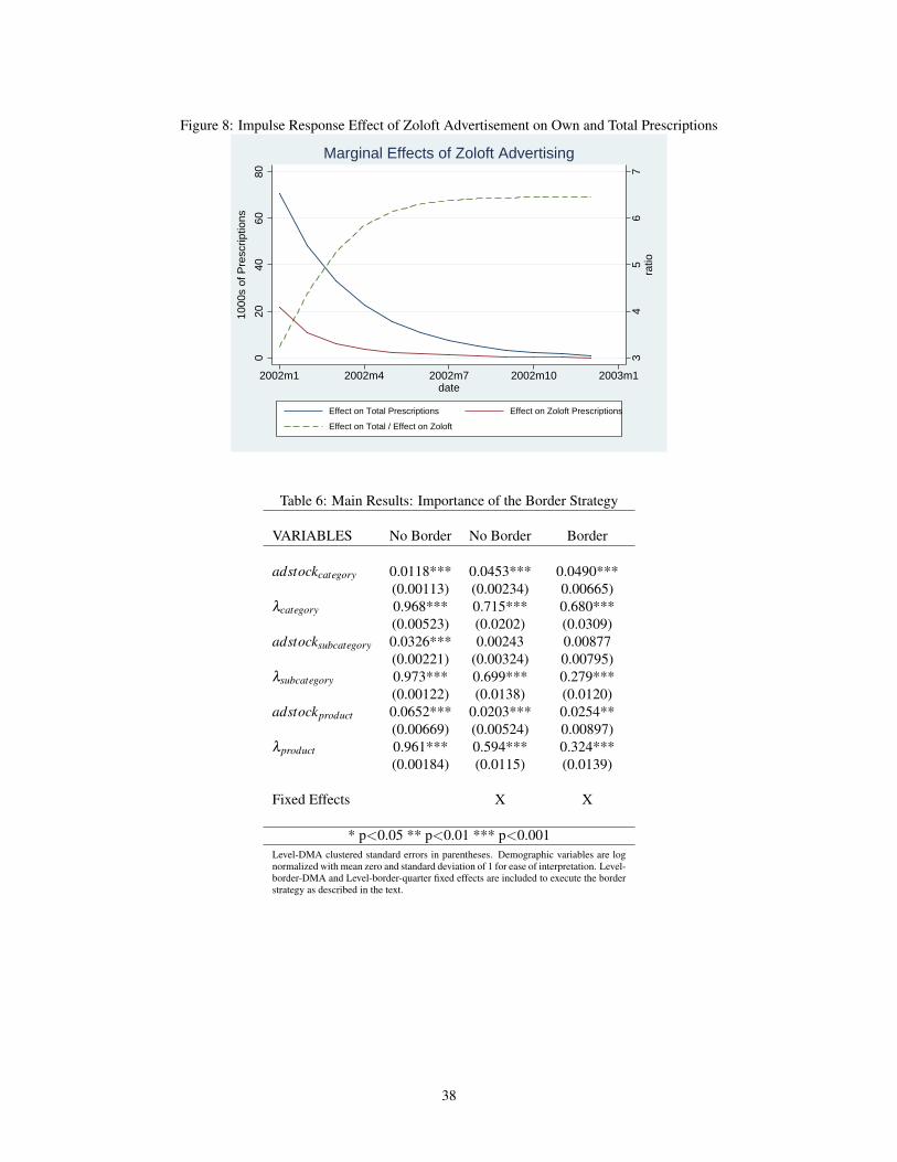
Figure 8: Impulse Response Effect of Zoloft Advertisement on Own and Total Prescriptions

34

56

7ra

tio

020

4060

80

1000

s of

Pre

scrip

tions

2002m1 2002m4 2002m7 2002m10 2003m1date

Effect on Total Prescriptions Effect on Zoloft Prescriptions

Effect on Total / Effect on Zoloft

Marginal Effects of Zoloft Advertising

Table 6: Main Results: Importance of the Border Strategy

VARIABLES No Border No Border Border

adstockcategory 0.0118*** 0.0453*** 0.0490***(0.00113) (0.00234) 0.00665)

λcategory 0.968*** 0.715*** 0.680***(0.00523) (0.0202) (0.0309)

adstocksubcategory 0.0326*** 0.00243 0.00877(0.00221) (0.00324) 0.00795)

λsubcategory 0.973*** 0.699*** 0.279***(0.00122) (0.0138) (0.0120)

adstockproduct 0.0652*** 0.0203*** 0.0254**(0.00669) (0.00524) 0.00897)

λproduct 0.961*** 0.594*** 0.324***(0.00184) (0.0115) (0.0139)

Fixed Effects X X

* p<0.05 ** p<0.01 *** p<0.001Level-DMA clustered standard errors in parentheses. Demographic variables are lognormalized with mean zero and standard deviation of 1 for ease of interpretation. Level-border-DMA and Level-border-quarter fixed effects are included to execute the borderstrategy as described in the text.

38

Tabl

e7:

Shor

tRun

Adv

ertis

ing

Ela

stic

ities

Prod

ucts

Paxi

lPa

xilC

RPr

ozac

Proz

acW

eekl

yW

ellb

utri

nSR

Wel

lbut

rin

XL

Zol

oft

Out

side

Opt

ion

Paxi

l0.

037

0.01

90.

021

0.01

90.

020

-0.

021

-0.0

23Pa

xilC

R0.

016

0.02

90.

016

0.01

60.

012

0.01

00.

016

-0.0

15Pr

ozac

0.00

92-

0.02

00.

0080

0.00

97-

0.00

92-0

.011

Proz

acW

eekl

y0.

0088

-0.

0088

0.01

80.

0068

-0.

0088

-0.0

080

Wel

lbut

rin

SR0.

014

-0.

014

0.01

20.

021

-0.

014

-0.0

14W

ellb

utri

nX

L0.

017

0.01

70.

017

0.01

70.

019

0.03

50.

017

-0.0

18Z

olof

t0.

013

0.01

30.

013

0.01

30.

013

0.01

00.

027

-0.0

15

39

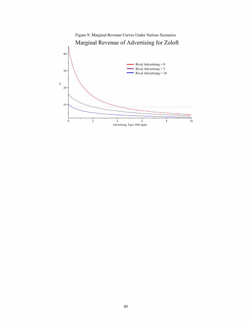
Figure 9: Marginal Revenue Curves Under Various Scenarios

40

Table 8: Evidence of Free Riding By Firms

VARIABLES DTC Log(DTC) 1(DTC>0) 1(DTC>0)

Rival DTC -0.0296*** -0.00334*(0.00240) (0.00160)

Log(RivalDTC) -0.0290***(0.00691)

1(RivalDTC>0) -0.0685***(0.0162)

Observations 39,414 39,414 39,414 39,414*** p<0.01, ** p<0.05, * p<0.1

Product-DMA clustered standard errors in parentheses. These regressions are run only for those products thatever advertise on TV. Product-DMA and Product-Quarter fixed effects are included as in the DMA-level demandanalysis.

Figure 10: MPE Simulation Advertising - Atlanta DMA

41

Figure 11: Realized Advertising - Atlanta DMA

01

23

45

Ad

$ P

er 1

00 C

apita

2000m1 2000m4 2000m7 2000m10 2001m1month

Prozac Paxil

Figure 12: MPE Simulation Profits - Atlanta DMA

42

Figure 13: Paxil/Prozac and Full Co-operative versus Competitive Total Advertising - Atlanta DMA

Figure 14: Paxil/Prozac Co-operative versus Competitive Total Profits - Atlanta DMA

43

Figure 15: Paxil/Prozac Co-operative versus Competitive Category Share - Atlanta DMA

Appendix A - Orthogonality of Pricing and Detailing Decisions

A.1 Pricing

The regression of television commercials on prices is shown in Table 9. As can be seen the point estimate is very smalland insignificant with respect to both own and cross advertising. The average unit price of a branded drug is about$3.24 over the course of the sample and the average DTC per capita for advertising products after September 1999is $0.65. The point estimate suggests that raising DTC per capita by $1 is associated with a price decrease of $0.05.This is very small economically. Interestingly, a time trend, a product fixed effect and a dummy for patent expirationcan explain prices with R squared larger than 0.99. Prices seem quite sticky, especially relative to advertising in thismarket.

44

Table 9: Predicting Prices with Advertising(1)

VARIABLES realunitprice

DTC -0.0518(0.0437)

RivalDTC -0.0332(0.0248)

time 0.00963***(0.00313)

expired -0.210(0.149)

Product FEs X

Observations 1188R-squared 0.994

*** p<0.01, ** p<0.05, * p<0.1Product Clustered Standard errors in parentheses

A.2 Detailing

To address the potential omitted variables bias problem associated with physician detailing, I use two data sources toshow that physician detailing is uncorrelated with DTC advertising. First, I use national level detailing informationfrom IMS health and exploit the law change that made DTC advertising feasible for pharmaceutical firms starting in1999. Using this data, I show that there is no trend break in firm detailing associated with the policy change, while thereis an enormous trend break in DTC, from zero to highly positive. Second, I employ data from ImpactRx that followsa panel of physicians through time, measuring the amount of detailing time was spent on them by drug. The dataincludes a panel of 2134 general practitioners and 167 psychiatrists that can be matched with the DTC and prescribingdata. These physicians are not representative of the population of physicians, as they are drawn disproportionatelyfrom the 40th percentile and higher in the prescribing distribution. ImpactRx does this because those below the 40thpercentile are much less likely ever to be detailed. While the 2301 physicians make up less than 1% of the populationof physicians, they are likely make up significantly more of the prescription share of the physician population. Forgeneral practitioners, the panel begins in 2001 and for psychiatrists, the panel begins in 2002 and includes geographicinformation. As such, the data is matched with a portion of the data used in the main analysis to test the robustnessof the identification to the inclusion of detailing. Detailing is measured in number of detail visits per product perphysician per month. With 101 DMAs in the data, this makes each DMA have an average of about 23 physicians inthis sample.

Using this data, I use two approaches to address the omitted variables bias concern. First, I aggregate the localdetailing measure to the DMA level and show that DTC and local detailing are not correlated conditional on the fixedeffects included in the model. Similarly, I aggregate the data to the border experiment level and show that this lack ofcorrelation extends to the border regions. Next, I include the border-experiment level detailing data in the model forthe limited months and experiments that can be matched and show that the exclusion of detailing has no effect on theestimates of DTC effectiveness.

45

Table 10 presents the results of the national-level analysis using IMS national detailing visit numbers. The regressionsare specified using product specific time trends, product fixed effects, a dummy to indicate that the product is in themarket, a dummy to indicate that the product’s patent has expired and a dummy for “post” September 1999, whenthe final FDA guidance was released. The coefficient on “post” will identify the average break in trend of detailingat the moment the law changes. The coefficient is small and positive, but insignificant. In contrast, using the samespecification but with DTC as the dependent variable in the second column, the “post” dummy shows a very largepositive and significant effect, as firms move from zero DTC advertising at the national level to a significant amountof DTC advertising. Even at the aggregate national level, it appears as though this major law change affecting firmstrategy has very little effect on the path of firm detailing decisions.

Table 10: Did the DTC Law Change Result in a Detailing Trend Break?

VARIABLES National Details National DTC

PostSept99 0.672 472***(0.796) (124)

Product Time Trend X XObservations 992 992R-squared 0.932 0.266

*** p<0.01, ** p<0.05, * p<0.1Standard errors in parentheses. Included in each specification are product fixed effects,product specific time trends, a dummy indicating a product’s patent has expired and adummy indicating that the product is in the market. Average detailing per month in thesample is 16.807. Average national DTC per month in the sample is 427.750

The next strategy employed to assess the potential for bias is to aggregate the physician-level detailing from ImpactRxto the DMA level. Since DTC advertising is decided at the DMA level and no more local, I want to test if detailingdecisions are sensitive to DTC decisions at the DMA level. I regress own local DTC and rival local DTC, measured indollars per hundred capita on product detailing visits in the DMA. Similar to the main specification, I include product-quarter and product-DMA fixed effects. I want to know within time period and within DMA, if higher DTC for oneproduct associated with higher detailing. The results of the regression are presented in the first column of Table 11. Asit turns out, there is no statistically significant relationship between either own or rival DTC and detailing decisions.This is consistent with conversations with managers who said that detailing and DTC decisions are made in differentdivisions of the firm and coordination very difficult. While the estimates are not statistically significant, it is worthnoting that even if they were, the magnitudes of the point estimates are very small. The standard deviation of localDTC campaigns is 0.17. Taken at face value, an increase in own local DTC of one standard deviation is associatedwith an increase in detailing visits for doctors in this sample in the DMA by about 0.1. Extrapolating this point basedon the size of the sample, the point estimate would imply an average of about 1 additional detailing visit per 230physicians associated with a one standard deviation increase in local DTC. The point estimate on rival advertising iseven smaller. This provides evidence that widespread strategies to undercut rival DTC with detailing campaigns arenot prevalent.

In the second column of Table 11, the same exercise is run at the border-experiment level. The results are broadlysimilar, though these results should be taken with a grain of salt as each observation is based on far fewer physiciansat this narrow level of analysis. However, there is no evidence that detailing efforts change sharply at borders whereone side has significantly higher DTC.

46

Table 11: Are Detailing Campaigns Coordinated with DTC?

DMA Level Border-Experiment LevelVARIABLES Detailing Visits Detailing Visits

Local DTC 0.662 0.579(0.475) (0.490)

Rival Local DTC 0.184 0.0326(0.177) (0.108)

Observations 22,589 18,622R-squared 0.764 0.789

*** p<0.01, ** p<0.05, * p<0.1Product-DMA clustered standard errors in parentheses. Column 1 presents DMA level analysiswhile Column 2 provides border experiment level analysis. They contain the same fixed effectsas those in the demand models of the same level.

The final strategy used to think about this problem is to directly incorporate local detailing data into the main analysis.Detailing data is aggregated to the product-border-DMA-time level as with the main specification. Since the physicianpanel in the detailing data is smaller in both number of physicians and in length of time, the matched sample will besubstantially smaller and over a shorter time frame than the main specification. As such, there is no longer sufficientlylarge T to ensure that the lagged dependent variable Nickel bias is small. The persistence parameters will all be biaseddownward in these specifications. The main goal of this exercise is to see if the coefficients on DTC are robust to theinclusion of detailing.

The effect of including detailing in this model is demonstrated in Tables 12 and 13 . Both tables include all matcheddata from 2001 onwards. The regressions in Table 12 include the log of detailing visits while the regressions in Table13 do not. Table 12 presents specifications that both include and exclude interaction terms between DTC and detailing.As we can see, the effects of DTC are not significantly affected by the exclusion of detailing or the interactions ofDTC with detailing. As expected, the persistence parameters are all much smaller than in the main model in Table 5due to the smaller number of time periods.

These exercises show that over the course of the time period where detailing data is available in this class, detailingis not significantly correlated with DTC at either the DMA level or the border experiment level. Further, includingdetailing in the main model does not change the main parameters of interest. While this paper makes no claims ofidentifying the causal effects of detailing, it seems as though it poses a minimal threat to the identification of the causaleffect of DTC using the border strategy.

Appendix B - Placebo Test

With a difference-in-differences model, the assumption of parallel trends in the outcome variable absent the treatmentis required for a valid estimation. One way to assess the validity of this assumption is through the use of a placebotest. In this case, I will use advertising for over-the-counter (OTC) sleep aids as a placebo treatment. This is an idealplacebo for two reasons: first, it varies at the same level as antidepressant advertising- at the DMA month. Next, OTCsleep aids need not be prescribed by a physician, so we should not expect a “going to the doctor” effect of advertising

47

Tabl

e12

:Res

ults

ofL

imite

dM

odel

Incl

udin

gG

eogr

aphi

cD

etai

ling

from

2001

On

VAR

IAB

LE

SC

ateg

ory

Lev

elC

ateg

ory

Lev

elSu

bcat

egor

yL

evel

Subc

ateg

ory

Lev

elPr

oduc

tLev

elPr

oduc

tLev

el

adst

ock

0.04

84**

*0.

0474

**0.

0034

50.

0071

00.

0300

**0.

0314

**(0

.006

38)

(0.0

0730

)(0

.009

22)

(0.0

0968

)(0

.010

3)(0

.010

5)Lo

gVis

its

0.00

570

0.00

806

-0.0

0471

0.00

029

0.00

236

0.00

378

(0.0

0578

)(0

.008

06)

(0.0

0568

)(0

.007

33)

(0.0

0358

)(0

.003

62)

LogV

isit

s×ad

stoc

k0.

0015

7-0

.006

82-0

.005

58(0

.003

57)

(0.0

0485

)(0

.006

59)

pers

iste

nce

0.48

9***

0.48

9***

0.12

4***

0.12

4***

0.26

0***

0.26

0***

(0.0

497)

(0.0

496)

(0.0

146)

(0.0

146)

(0.0

153)

(0.0

153)

Obs

erva

tions

9,86

19,

861

42,8

6042

,860

77,8

9177

,891

R-s

quar

ed0.

960

0.96

00.

940

0.94

00.

968

0.96

8**

*p<

0.01

,**

p<0.

05,*

p<0.

1L

evel

-DM

Acl

uste

red

stan

dard

erro

rsin

pare

nthe

ses.

Dem

ogra

phic

inte

ract

ions

incl

uded

asin

the

mai

nan

alys

isbu

tsu

ppre

ssed

fore

xpos

ition

alcl

arity

.

48

Table 13: Results of Limited Model Without Geographic Detailing

VARIABLES Category Level Subcategory Level Product Level

adstock 0.0491*** 0.00301 0.0301***(0.00636) (0.00911) (0.00103)

persistence 0.489*** 0.124*** 0.260***(0.0497) (0.0146) (0.0153)

Observations 9,861 42,860 77,891R-squared 0.960 0.940 0.968

*** p<0.01, ** p<0.05, * p<0.1DMA clustered standard errors in parentheses. Demographic interactions included as in the main analysisbut suppressed for expositional clarity.

to be present in OTC advertising. I will use the same identification strategy, but I will use OTC sleep aid advertising asa treatment. The results are presented in Table 14. None of the coefficients on OTC sleep aid advertising is statisticallysignificant at the 5% level or economically important at any level.

Table 14: Results of Base Model with Placebo

VARIABLES Category Level Subcategory Level Product Level

OTCSLEEPAD 0.0000565 0.000471 0.00218*(0.000397) (0.000482) (0.00113)

persistence 0.684*** 0.280*** 0.323***(0.0304) (0.0116) (0.0139)

Observations 22,826 93,280 147,443R-squared 0.948 0.935 0.960

*** p<0.01, ** p<0.05, * p<0.1Level-DMA clustered standard errors in parentheses

Appendix C - Alternative Sample Selection

One might worry that the effect of advertising in the border sample counties differs systematically from the non-bordercounties or that the effect of advertising in rural areas would be much different than the effect of advertising in urbanareas. To think about these concerns, I have repeated the analysis with several alternative sample selections.

C.1 The Urban Rural Divide

C.1.1 Without the Northeast Corridor and Other Urban Areas

It seems the less urban areas show very similar results to the full border sample. The category and product level effectsare larger, but not significantly different from the full sample of borders.

49

Table 15: Results of Base Model without Northeast Corridor and Other Urban Areas

VARIABLES Category Level Subcategory Level Product Level

adstock 0.0508*** 0.00874 0.0279***(0.00825) (0.00904) (0.00939)

persistence 0.689*** 0.255*** 0.313***(0.0322) (0.0129) (0.0159)

Observations 17,400 67,976 99,101R-squared 0.946 0.927 0.955

*** p<0.01, ** p<0.05, * p<0.1Level-DMA clustered standard errors in parentheses

C.1.2 Only the Urban Border Counties

It seems the effects of advertising are a bit smaller in the more urban areas, except at the nest level. However, it seemsmore likely that the identifying assumption might fail in the more urban areas, as the borders are much closer to thecentral cities than in the more rural borders.

Table 16: Results of Base Model with only Northeast Corridor and Other Urban Areas

VARIABLES Category Level Subcategory Level Product Level

adstock 0.0348*** 0.0191** 0.00707***(0.00951) (0.00940) (0.0111)

persistence 0.648*** 0.387*** 0.381***(0.0678) (0.0215) (0.0284)

Observations 5,775 25,550 41,586R-squared 0.963 0.956 0.972

*** p<0.01, ** p<0.05, * p<0.1Level-DMA clustered standard errors in parentheses

C.2 The “Anti” Border Sample

Here, I use all of the counties that are not in the border sample. For this sample, endogeneity should be the most severe.The results of this estimation should reveal the main drivers of the endogeneity problem that necessitates use of theborder sample. If the main effects of advertising are much larger in this estimation, it would lead us to believe thatadvertising was strongly correlated with unobserved local demand shocks such as weather shocks, employment shocksor special seminars that are unobserved. These shocks, if positively correlated with advertising decisions would leadus to falsely conclude that the effect of advertising is high. If, on the other hand, the reverse causality concern- wherefirms target an advertising to sales ratio based on sales in the previous period, we would expect that in the anti-bordersample the persistence parameter would be much higher. That is, lagged shares would not only be measuring thepersistence of prescribing associated with advertising carry-over, they would also be controlling for the rule of thumbdecision of firms to target DMAs that had large shares in the previous period. Results of the estimation are in Table

50

14. As can be seen, while the point estimates on advertising do not significantly change from the border sample, theyare larger, and the persistence parameters are much (and significantly) larger. This suggests that the main source ofendogeneity is reverse causality- if firms are following a rule of thumb advertising to sales ratio based on previousperiod sales, the lagged share variable will be biased upward as it controls for the firm’s rule of thumb rather thanestimating persistence.

Table 17: Results of Base Model Using the “Anti”-Border Approach

VARIABLES Category Level Subcategory Level Product Level

adstock 0.0508*** 0.0049 0.0182***(0.00164) (0.00251) (0.00439)

persistence 0.751*** 0.721*** 0.594***(0.0259) (0.0128) (0.0115)

Observations 8,466 42,181 73,628R-squared 0.981 0.984 0.984

*** p<0.01, ** p<0.05, * p<0.1Level-DMA clustered standard errors in parentheses

C.3 Removing the State Borders

As described in the text, if tax rates cause a selection problem of physicians into DMAs, then results could be biased.To assess this possibility, DMA borders which coincide with state borders are removed from the sample. That removesroughly one third of the borders in the sample. The analysis is re-run using the set of DMA borders that do not coincidewith state borders. Results are available in Table 17. The results are very similar and not statistically distinguishablefrom those in the full sample.

Table 18: Results of Base Model Without State Border Overlap

VARIABLES Category Level Subcategory Level Product Level

adstock 0.0376*** 0.0131* 0.0256***(0.00764) (0.00783) (0.00881)

persistence 0.683*** 0.271*** 0.327***(0.0368) (0.0133) (0.0166)

Observations 15,975 65,097 97,720R-squared 0.981 0.984 0.984

*** p<0.01, ** p<0.05, * p<0.1Level-DMA clustered standard errors in parentheses

Appendix D - Primary Care Service Areas

As mentioned in section (3.1.1), measurement error could bias my estimates towards zero if patients are going to thedoctor in different counties than where they watch television advertisements. The Dartmouth Center for Health Policy

51

Research has developed a Primary Care Service Area (PCSA) project which is the first national database of primarycare resources for small areas. These areas were defined using Medicare claims data from 1999 and Census data from2000. The service areas include a ZIP area with one or more primary care providers and any bordering ZIPs where thepopulation largely gets their primary care from those physicians.

This database allows me to ask how many patients travel across DMA borders to seek their primary care. In particular,I can match this data to my prescribing data at the ZIP level. I can then see what percentage of each PCSA falls intoa single DMA. Doing this I find that only about 1% of PCSAs cross DMA borders at all. Of those that do cross DMAborders, they do so only minimally. That is, the DMA holding the majority of a PCSA which crosses a border onaverage contains 97% of that PCSA. As such, measurement error bias should be minimal.

While this only holds for Medicare beneficiaries and primary care physicians, it should be noted that primary carephysicians do make up a large portion, on the order of 80% of antidepressant prescriptions.14 For this to be a large mea-surement error issue, non-Medicare recipients must travel larger distances than Medicare recipients to their physicians.To the extent that this is true, it will lead to measurement error that biases all estimates of advertising effectivenesstowards zero.

Appendix E - Selection of Households and Physicians to Counties

E.1

It might present a problem if households and physicians pre-disposed to be more affected by advertisements system-atically select into border counties on the side of the border that receive more advertisements. This is a difficult levelof selection to address. However, I do check for balance in characteristics across the borders. First, I check to see ifphysicians are more likely to bunch on the “high DTC” side of the border. To do this, I collected data from the AreaResource File from 2001 that contained information on the number of physicians in a particular county- I collectedthis data for both total number of physicians and non-federal physicians. To determine the “high DTC” side of theborder, I totaled the local ads from 2001 for each side of a particular border. If one side saw more advertising in totalin 2001, it is called the “high DTC” side. I then ran a t-test to see if the means of the numbers of physicians were thesame on either side of the border. The t-test fails to reject that the number of physicians is the same on either side ofthe border, with p=0.21 for total doctors and p=0.25 for non-federal doctors.

Next, we might be concerned that the counties on the “high DTC” side of the border are systematically higher incomeor higher population than those on the “low DTC” side of the border. A t-test fails to reject that average income is thesame across the border, with p=0.47. Similarly, a t-test for population fails to reject that the populations are the sameacross the border with p=0.17.

Results for all of these tests are presented in Table 18. It should be noted that the market fixed effects in the model allowfor different levels in all of these variables so long as the trends are parallel and that the effectiveness of advertising isthe same across the border. That there does not seem to be systematic differences in characteristics across the borderfurther solidifies that this level of comparison is a reasonable one.

14http://psychcentral.com/news/2011/08/08/more-antidepressants-prescribed-by-non-psychiatrists/28423.html.

52

Table 19: Tests for Selection Across Borders

variable high DTC low DTC t-stat p-value

Physicians 855 715 1.25 0.215(136) (124)

Non-Fed Physicians 98.8 88.0 1.15 0.252(12.9) (11.3)

Income 24,162 23,881 0.723 0.471(460) (399)

Population 1,150,642 979,142 1.37 0.173(168,114) (180,925)

N = 153 border clustersMeans Above Standard Errors in Parentheses

E.2

We might also worry that the border counties are systematically different from non-border counties in observable ways.This would hurt the generalizability of the results. As such, I compare border counties to interior counties in termsof the average number of doctors, the average number of non-federal doctors, the average population and the averageincome in Table 19. These comparisons are at the county level rather than at the border cluster as in the previouscomparison, so there are many more observations.

Table 20: Tests for Observable Selection into Border Sample

variable Border Sample Non Border Sample t-stat p-value

Physicians 297.404 330.548 0.792 0.428(864.491) (1175.56)

Non-Fed Physicians 34.827 36.932 0.553 0.580(81.697) (99.333)

Income 24,203 24,413 0.763 0.446(6249) (6201)

Population 127,310 123,482 0.286 0.774(287,262) (346,498)

N=664 border, N=2221 non-borderMeans Above Standard Errors in Parentheses

Appendix F - Framework for Simulating The Size of the Incentive Effects

F.1 Supply

Firm free riding may be an optimal strategy in a game with positive spillovers. To investigate the incentives generatedby the demand problem above, we would like to measure the marginal revenues generated by this type of advertising

53

and compare those with the marginal costs. Since advertising has a dynamic effect through carry-over, one mustincorporate the dynamics through solving a dynamic programming problem. I should note here that the purpose ofthis exercise is not to predict firm behavior but to illustrate the size of the incentive effects of advertising spillovers. Todo this, I will assume a very stylized model where firms optimize profits only over advertising and are forced to holdpricing and detailing fixed.

I assume that firms play a simultaneous game, choosing advertising each period while taking into account expectationsof rival behavior and the dynamic effects of advertising. This enables me to analyze the magnitude of potential under-provision levels on average generated by positive spillovers in a very stylized game where only DTC advertising ismoving.

F.1.1 The Firm’s Problem

A forward looking firm maximizes a discounted stream of future profits with respect to advertising. Suppose advertis-ing has a constant marginal cost k jm, the market size is µm , prices are p j, marginal production costs are mc j and thediscount rate is β . Further, suppose the exogenously given set of products that a firm f has in the market is denotedby Φ f and the full set of products in the market is denoted by ∪ f Φ f .

Per period profit for the firm will be a function of advertising stock at the product, subcategory and category levelAmt ={A jmt , Anmt , Almt}, which is a function of the vector of current advertising for all products, amt , advertisingstocks in the previous period Am,t−1, and persistence parameters λ j, λn, and λI . Per period profit is also a functionother variables X , a constant marginal cost of advertising k jmt , and product-market-time specific iid demand shocks ξ :

π f mt = ∑j∈Φ f

(p jt −mc jt)µmts jmt(Amt , X , ξ )− k jmta jmt .

The firm’s problem is to maximize the stream of future profits for all products in its portfolio. Advertising is set priorto the realization of any demand shocks, so only expected profits matter for firm choices. Expected per period profitsare:

π f mt = ∑j∈Φ f

ˆ(p jt −mc jt)µmts jmt(Amt , X , ξ )p(ξ )dξ − k jmta jmt . (28)

The timing of the game is as follows. At the start of each period, the state of the market gmt, is revealed to all firms.Based on that state, firms will make advertising decisions σ jm(gmt) = a jmt . The state variables could include anythingin the past history of the game, but I will restrict attention to games where payoff-relevant state variables are the onlyones that matter. Given the demand system provided above, state variables will include only the current advertisingstock Amt ={A jt , Anmt , Almt}. After the state variables are observed, the firm makes its advertising decision, thecurrent period demand shocks are realized and the firms collect their profits for the period.

The strategy profile σ = (σ1, ..., σJ) contains the decision rules of the firms. Firm f ’s expected present discountedvalue of all profits given the current state gmt and the full strategy profile σ is

54

Vf m(gmt|σ) = E[∞

∑j∈Φ f

∞

∑τ=t

βτ−t

π f (gms, σ f (gms))|gmt]. (29)

Firm f chooses a sequence of advertising levels σ f , which are state dependent, to maximize Vf m(gmt|σ). I will assumethat firms form expectations regarding future states and thus future strategies given current period state variables. Assuch, firm f will have a Markov strategy, σ f m : g→ σ f (g) = (a jm)∀ j∈Φ f . To assess the strategies of competitors, firmf makes an assumption about σ− f and chooses σ f .

The equilibrium concept used will be Markov perfect equilibrium. A Markov perfect equilibrium is a set of strategiesthat form a subgame perfect equilibrium where strategies may only be conditioned on payoff relevant state variablesand on the current state of the game. In particular,

σ∗f ∈ argmax{Vf m(gmt|σ)} (30)

for all states gmt, firms f , and actions a jm. That is, each firm will maximize the discounted sum of expected profitsgiven beliefs about competitors behavior, and each firm’s beliefs are mutually consistent in equilibrium. Using MPEmakes the allowable strategy space relatively simple. I will further restrict attention to pure strategies in advertising.Firms will use the Bellman equation to solve the dynamic programming problem:

Vj(g|σ) =sup

a ∈ R+{π j(g, a, σ− j(g))+βEV (g′|σ)} (31)

F.2 MPE Simulation

I solve the Markov Perfect Equilibrium (MPE) of the advertising game using a policy iteration algorithm, similar toDube et. al. 2005. I take an initial guess of the strategy profile σ0 = (σ0

1 , ...,σ0J ), and then take the following steps:

1. For the strategy profile σn, calculate the value functions for each of the J firms, V nj . The value functions are

defined by the Bellman equation (31). In this step, the maximization on the right hand side is not carried out,but the current guess of σnis plugged in.

2. For all n > 0, check whether the value functions and policy functions satisfy pre-determined convergence crite-ria, ||V n

j −V n−1j ||< εV and ||σn

j −σn−1j ||< εσ . If so, stop the process.

3. Update each firm’s strategy using the Bellman equation (31). Do this by carrying out the optimization on theright hand side. Denote the resulting policies and value functions by σn+1and V n+1. Return to step 1.

The value functions are represented on a grid. As in the supply simulation, there are two firms, there are two firmadvertising stocks and a category advertising stock. That makes three state variables. The grid is 5x5x5. Outside ofthe grid, the value function is determined using bilinear interpolation.

55

For the two-firm co-operative counterfactual, the MPE simulation turned into basically a monopoly game simula-tion where both firms’ profits are considered and no other firms advertise. For the full co-operative counterfactual,computation is the same, only the advertising firm considers the profits of all products on the market.

Using the derived policies in each of these computations, the equilibria are simulated forward given the market initialconditions to generate the figures.

Available at Request - LDV Simulation

As there is a concern that a lagged dependent variable (LDV) will have a biased estimate with fixed effects in a panelmodel due to correlation between the lagged dependent variable and the error term, the purpose of this appendix is tosimulate the size of such a bias. The theoretical size of the bias is computed in the text, but that only holds as N→ ∞.The finite sample simulation will assess how good of an approximation that is. In particular, I assume that the datagenerating process is:

• λcategory = 0.68

• αcategory = 0.0494

• λsubcategory = 0.28

• αsubcategory = 0.00662

• λproduct = 0.324

• αproduct = 0.025

With product-border-market, product-border-time, subcategory-border-market, subcategory-border-time, category-border-market and category-border-time fixed effects drawn from random normal distributions initially, all mean zero and themarket effects with standard deviation of 1 and time effects standard deviations of 0.5.

Using 500 draws of epsilons with standard deviations that match the residual standard deviations of product, subcate-gory and category dependent variables, I simulate data, estimate the parameters using the same methods described inthe paper. I then compute the difference between the estimated parameters and the true values that I set, λ̂l −λl andα̂l−αl . The results of the simulation are as follows:

Table 21: Simulated LDV Bias

Variable Mean SD

(λ̂category−λcategory) -0.0208 0.00258(α̂category−αcategory) -0.000790 0.00598(λ̂subcategory−λsubcategory) -0.0401 0.00171(α̂subcategory−αsubcategory) 0.00132 0.00933(λ̂product −λproduct) -0.0223 0.000911(α̂product −αproduct) 0.00009 0.00450

56