Marnix van Berchum; The art of sharing: open acces - open arts

Portfolio Optimization:Beyond Markowitz
Master’s Thesis by
Marnix Engels
January 13, 2004


Preface
This thesis is written to get my master’s title for my studies mathematics atLeiden University, the Netherlands. My graduation project is done during aninternship at Rabobank International, Utrecht, where I have been from May tillDecember 2003.
At the beginning of the internship, it was quite a shift to start thinking inbanking terms, where I was used to reason in a pure mathematical context. Butas with most things in life, with a lot of curiosity, patience and perseverancea nice result can be made. I have learned a lot during the internship. It wassurprising for me how much of the four-year mathematical studies I was ableto use in the banking world. Optimizing, statistics, linear algebra, second ordercone programming and the use of MATLAB are just a few subjects I used duringthe last seven months.
My special thanks goes to Mace Mesters for guiding me throughout theinternship and for teaching me there are always more articles to read. I alsolike to thank my roommates Walter Foppen (for playing DJ Foppen, Walter degekste!) and Harmenjan Sijtsma (for getting tea all the time) and teammateMartijn Derix (for installing a lot of illegal software, essential for writing thisthesis, on my computer). For their helpful comments I thank Freddy van Dijk,Erik van Raaij, Roger Lord, Natalia Borovykh, Adriaan Kukler, Marion Segeren,Erwin Sandee, Rik Albrecht and Sacha van Weeren. From Leiden University, Iwas supervised by prof. dr. L.C.M. Kallenberg, to whom I am very grateful.To conclude, thanks to my parents for supporting me throughout my studies,and I say hullo to Heidi.
Marnix EngelsLeiden, January 13, 2004
iii


Contents
Preface iii
List of figures viii
List of tables xi
List of symbols xiii
1 Introduction 1
2 The portfolio theory of Markowitz 5
2.1 Efficient frontier . . . . . . . . . . . . . . . . . . . . . . . . . . . 52.2 Minimum variance portfolio . . . . . . . . . . . . . . . . . . . . . 82.3 Tangency portfolio . . . . . . . . . . . . . . . . . . . . . . . . . . 92.4 Optimal portfolio . . . . . . . . . . . . . . . . . . . . . . . . . . . 112.5 Adding a risk-free asset . . . . . . . . . . . . . . . . . . . . . . . 14
2.5.1 Capital market line & market portfolio . . . . . . . . . . . 142.5.2 Optimal portfolio . . . . . . . . . . . . . . . . . . . . . . . 16
2.6 Sensitivity analysis . . . . . . . . . . . . . . . . . . . . . . . . . . 182.7 Example . . . . . . . . . . . . . . . . . . . . . . . . . . . . . . . . 20
2.7.1 Data . . . . . . . . . . . . . . . . . . . . . . . . . . . . . . 202.7.2 Calculations . . . . . . . . . . . . . . . . . . . . . . . . . . 23
2.8 References . . . . . . . . . . . . . . . . . . . . . . . . . . . . . . . 26
3 Another aproach for risk: Safety first 27
3.1 Safety first models . . . . . . . . . . . . . . . . . . . . . . . . . . 273.2 Telsers criterion . . . . . . . . . . . . . . . . . . . . . . . . . . . . 28
3.2.1 Formulation . . . . . . . . . . . . . . . . . . . . . . . . . . 283.2.2 Intuitive solution . . . . . . . . . . . . . . . . . . . . . . . 293.2.3 Analytical solution . . . . . . . . . . . . . . . . . . . . . . 30
v

3.3 With risk-free asset . . . . . . . . . . . . . . . . . . . . . . . . . . 303.3.1 Intuitive solution . . . . . . . . . . . . . . . . . . . . . . . 303.3.2 Analytical solution . . . . . . . . . . . . . . . . . . . . . . 32
3.4 Example . . . . . . . . . . . . . . . . . . . . . . . . . . . . . . . . 323.5 References . . . . . . . . . . . . . . . . . . . . . . . . . . . . . . . 35
4 Elliptical distributions 37
4.1 Introduction . . . . . . . . . . . . . . . . . . . . . . . . . . . . . . 374.2 Some examples of elliptical distributions . . . . . . . . . . . . . . 39
4.2.1 Normal family . . . . . . . . . . . . . . . . . . . . . . . . 394.2.2 Student-t family . . . . . . . . . . . . . . . . . . . . . . . 394.2.3 Laplace family . . . . . . . . . . . . . . . . . . . . . . . . 404.2.4 Logistic family . . . . . . . . . . . . . . . . . . . . . . . . 414.2.5 Differences and similarities . . . . . . . . . . . . . . . . . 42
4.3 Mean-variance analysis . . . . . . . . . . . . . . . . . . . . . . . . 444.4 Telser and elliptically distributed returns . . . . . . . . . . . . . . 464.5 Example . . . . . . . . . . . . . . . . . . . . . . . . . . . . . . . . 484.6 References . . . . . . . . . . . . . . . . . . . . . . . . . . . . . . . 51
5 Value at Risk based optimization 53
5.1 VaR efficient frontier . . . . . . . . . . . . . . . . . . . . . . . . . 535.2 Adding the risk-free asset . . . . . . . . . . . . . . . . . . . . . . 585.3 Optimal portfolios . . . . . . . . . . . . . . . . . . . . . . . . . . 59
5.3.1 Minimum Value at Risk portfolio . . . . . . . . . . . . . . 595.3.2 Tangency VaR portfolio . . . . . . . . . . . . . . . . . . . 605.3.3 Telser . . . . . . . . . . . . . . . . . . . . . . . . . . . . . 615.3.4 Telser with risk-free asset . . . . . . . . . . . . . . . . . . 63
5.4 Example . . . . . . . . . . . . . . . . . . . . . . . . . . . . . . . . 645.5 References . . . . . . . . . . . . . . . . . . . . . . . . . . . . . . . 70
6 Maximizing the performance measures EVA and RAROC 73
6.1 EVA and RAROC . . . . . . . . . . . . . . . . . . . . . . . . . . 736.2 New Telser models . . . . . . . . . . . . . . . . . . . . . . . . . . 74
6.2.1 EVA with allocated capital . . . . . . . . . . . . . . . . . 746.2.2 EVA with consumed capital . . . . . . . . . . . . . . . . . 756.2.3 RAROC with allocated capital . . . . . . . . . . . . . . . 796.2.4 RAROC with consumed capital . . . . . . . . . . . . . . . 796.2.5 Comparison EVA-RAROC . . . . . . . . . . . . . . . . . . 80
6.3 Models with risk-free asset . . . . . . . . . . . . . . . . . . . . . . 826.3.1 EVA . . . . . . . . . . . . . . . . . . . . . . . . . . . . . . 826.3.2 RAROC . . . . . . . . . . . . . . . . . . . . . . . . . . . . 83
6.4 Example . . . . . . . . . . . . . . . . . . . . . . . . . . . . . . . . 846.5 References . . . . . . . . . . . . . . . . . . . . . . . . . . . . . . . 85
7 Modeling uncertainty of input parameters 87
7.1 Overview . . . . . . . . . . . . . . . . . . . . . . . . . . . . . . . 877.2 Uncertainty sets . . . . . . . . . . . . . . . . . . . . . . . . . . . 887.3 Second order cone programming . . . . . . . . . . . . . . . . . . 887.4 Portfolio optimization and SOCP . . . . . . . . . . . . . . . . . . 90
7.4.1 Markowitz . . . . . . . . . . . . . . . . . . . . . . . . . . . 90
vi

7.4.2 Telser . . . . . . . . . . . . . . . . . . . . . . . . . . . . . 917.5 Portfolio optimization with uncertainty . . . . . . . . . . . . . . 91
7.5.1 Markowitz . . . . . . . . . . . . . . . . . . . . . . . . . . . 917.5.2 Telser . . . . . . . . . . . . . . . . . . . . . . . . . . . . . 93
7.6 A more realistic approach . . . . . . . . . . . . . . . . . . . . . . 947.6.1 Markowitz . . . . . . . . . . . . . . . . . . . . . . . . . . . 957.6.2 Telser . . . . . . . . . . . . . . . . . . . . . . . . . . . . . 95
7.7 Example . . . . . . . . . . . . . . . . . . . . . . . . . . . . . . . . 967.7.1 Uncertainty sets . . . . . . . . . . . . . . . . . . . . . . . 967.7.2 Calculations . . . . . . . . . . . . . . . . . . . . . . . . . . 98
7.8 References . . . . . . . . . . . . . . . . . . . . . . . . . . . . . . . 100
8 Conclusion 103
8.1 Concluding example . . . . . . . . . . . . . . . . . . . . . . . . . 1038.2 Future research . . . . . . . . . . . . . . . . . . . . . . . . . . . . 105
Appendices 106
A Some large calculations 107
A.1 The market portfolio . . . . . . . . . . . . . . . . . . . . . . . . . 107A.2 The Telser portfolio . . . . . . . . . . . . . . . . . . . . . . . . . 109A.3 The Value at Risk efficient frontier . . . . . . . . . . . . . . . . . 109
B Telser portfolio analytical 111
B.1 No risk-free asset . . . . . . . . . . . . . . . . . . . . . . . . . . . 111B.2 With risk-free asset . . . . . . . . . . . . . . . . . . . . . . . . . . 114
C MATLAB programs 117
C.1 robustmarkowitz.m . . . . . . . . . . . . . . . . . . . . . . . . . . 117C.2 robusttelser.m . . . . . . . . . . . . . . . . . . . . . . . . . . . . . 118C.3 robustmarkowitz2.m . . . . . . . . . . . . . . . . . . . . . . . . . 119C.4 robusttelser2.m . . . . . . . . . . . . . . . . . . . . . . . . . . . . 119
vii


List of Figures
2.1 The efficient frontier . . . . . . . . . . . . . . . . . . . . . . . . . 72.2 The minimum variance portfolio . . . . . . . . . . . . . . . . . . 92.3 The tangency portfolio . . . . . . . . . . . . . . . . . . . . . . . . 102.4 The optimal portfolio . . . . . . . . . . . . . . . . . . . . . . . . 122.5 The market portfolio and Capital Market Line . . . . . . . . . . 14
2.6 The optimal portfolio with risk-free asset . . . . . . . . . . . . . 172.7 Overview of indexed returns of seven members of Dutch AEX-index 222.8 Graphical view of the portfolios of the example . . . . . . . . . . 26
3.1 The feasible area A and the optimal Telser point . . . . . . . . . 293.2 The optimal Telser portfolio with risk-free asset . . . . . . . . . . 31
3.3 Graphical view of the Telser portfolio of this example . . . . . . 34
4.1 Marginal and bivariate standard normal density function . . . . . 404.2 Marginal and bivariate student-t density functions . . . . . . . . 414.3 Marginal and bivariate Laplace density functions . . . . . . . . . 424.4 Marginal and bivariate Logistic density functions . . . . . . . . . 43
4.5 Comparison of four elliptical distributions . . . . . . . . . . . . . 434.6 Enlargement of the righthand tail . . . . . . . . . . . . . . . . . . 444.7 The Telser portfolios with different elliptical distributions . . . . 50
5.1 Definition of Value at Risk . . . . . . . . . . . . . . . . . . . . . . 54
5.2 The efficient frontier in mean-standard deviation and mean-VaRframework . . . . . . . . . . . . . . . . . . . . . . . . . . . . . . . 57
5.3 Graphical relationship of the efficient frontier in mean-st.dev. andmean-VaR framework. . . . . . . . . . . . . . . . . . . . . . . . . 57
5.4 Graphical relationship of the CML in mean-st.dev. and mean-VaR framework. . . . . . . . . . . . . . . . . . . . . . . . . . . . 58
5.5 The minimum VaR portfolio . . . . . . . . . . . . . . . . . . . . . 60
ix

5.6 The minimum VaR portfolio . . . . . . . . . . . . . . . . . . . . . 615.7 The optimal Telser portfolio . . . . . . . . . . . . . . . . . . . . . 625.8 The optimal Telser portfolio with risk-free asset . . . . . . . . . . 635.9 QQ-plots of Elsevier, Fortis, Getronics and Heineken. . . . . . . . 655.10 QQ-plots of Philips, Royal Dutch and Unilever. . . . . . . . . . . 665.11 Optimal Portfolios with VaR constraint. . . . . . . . . . . . . . . 70
6.1 Optimal ”EVA with allocated capital” portfolio . . . . . . . . . . 756.2 Moving the EVA-line with large rcap . . . . . . . . . . . . . . . . 766.3 Moving the EVA-line with small rcap . . . . . . . . . . . . . . . . 766.4 The tangency point is the Telser point . . . . . . . . . . . . . . . 776.5 Maximizing the slope of the RAROC-line . . . . . . . . . . . . . 796.6 The situation if the tangency Value at Risk exceeds V aRc . . . . 806.7 EVA maximization solutions with risk-free asset . . . . . . . . . . 826.8 RAROC maximization solutions with risk-free asset . . . . . . . 836.9 Optimal EVA and RAROC portfolios. . . . . . . . . . . . . . . . 86
7.1 The standard second order cone . . . . . . . . . . . . . . . . . . . 897.2 The optimal portfolios with uncertainty . . . . . . . . . . . . . . 997.3 The new efficient frontiers . . . . . . . . . . . . . . . . . . . . . . 100
x

List of Tables
1.1 The casino game . . . . . . . . . . . . . . . . . . . . . . . . . . . 1
2.1 Expected daily returns . . . . . . . . . . . . . . . . . . . . . . . . 212.2 Covariances of daily returns . . . . . . . . . . . . . . . . . . . . . 21
3.1 Yearly means, standard deviations and correlations . . . . . . . . 333.2 µ and Σ of yearly returns (×10−3) . . . . . . . . . . . . . . . . . 33
4.1 The quantiles kα for some elliptical distributions . . . . . . . . . 484.2 The quantiles kα for some elliptical distributions . . . . . . . . . 494.3 Optimal Telser allocation θ for different yearly distributions . . . 494.4 The optimal Telser allocation θ, with risk-free asset, for different
yearly distributions. . . . . . . . . . . . . . . . . . . . . . . . . . 50
5.1 Estimated left tail distribution of returns . . . . . . . . . . . . . 675.2 The quantiles for some elliptical distributions at different α . . . 675.3 Optimal Telser portfolio results with risk-free asset . . . . . . . . 70
6.1 Overview of the performance measures EVA and RAROC . . . . 74
7.1 Lower and upper bounds for means . . . . . . . . . . . . . . . . . 967.2 Lower and upper bounds for covariances . . . . . . . . . . . . . . 97
xi


List of Symbols
Symbols
n = number of assets.C0 = capital that can be invested, in euros.Cend = capital at the end of the period, in euros.Rp = total portfolio return, in euros.µp = expected portfolio return, in euros.σ2
p = variance of portfolio return.ri = rate of return on asset i.µi = expected rate of return on asset i.ρij = correlation between asset i and j.σij = covariance of asset i and j.
Σ =
σ11 σ12 . . . σ1n
σ21. . .
......σn1 . . . σnn
= matrix of covariances of r.
θi = amount invested in asset i, in euros.µf = rate of return on the risk-free asset.Rf = total return on the risk-free asset.γ = parameter of absolute risk aversion.s = slope of the capital market line in mean-st.dev.framework.kα = dispersion-standardized quantile of distribution at level α.zα = σ-standardized quantile of distribution at confidende level α.Ω = (n× n)-dispersion matrix.V aRα = Value at Risk at confidence level (1 − α).rcap = cost of capital rate.
xiii

Σ0 = (n× n)-matrix of average covariances.ΣL = (n× n)-matrix of lowest covariances.ΣU = (n× n)-matrix of highest covariances.∆ = ΣU − Σ0.µ0 = (n× 1)-vector of average means.µL = (n× 1)-vector of lowest means.µU = (n× 1)-vector of highest means.β = µU − µ0.‖ · ‖ = Euclidean norm.
r =
r1r2...rn
, µ =
µ1
µ2
...µn
, θ =
θ1θ2...θn
, 1 =
11...1
Expressions
With this symbols we can derive the following (logical) expressions. Notice thatthe vector notation is used throughout this thesis.
1. Cend = C0 +Rp.
2. Rp =∑n
i=0 riθi = rT θ.
3. µp =∑n
i=0 µiθi = µT θ.
4. σ2p =
∑ni=0
∑nj=0 θiθjσij = θT Σθ.
5. Rf = µfC0.
xiv

Chapter 1
Introduction
This thesis is about portfolio optimization. But what is an optimal portfolio?Consider the following example:
Suppose you are at the casino and there are two games to play. In the firstgame, there is a probability of 5% of winning 1000 euro and a 95% chance ofwinning nothing. The second game also has a 5 percent winning chance, butyou will win 5000 euro. On the contrary, if you lose, then you have to pay thecasino 200 euro. The facts are in the table below.
game I game II5%: +1000 euro 5%: +5000 euro
95%: 0 euro 95%: -200 euro
Table 1.1: The casino game
You are allowed to play the game once. Which game will you choose?
Most people will choose for game I. It is interesting to see why. The expectedreturn for the first game is (0.05× 1000) + (0.95 × 0) = 50, while the expectedreturn for game II is (0.05×5000)+(0.95×−200) = 60. Looking at the expectedreturn, it is more logical to play the second game! Nevertheless, in spite of thisstatistical fact, game I is the most popular. The explanation is that game IIappears to be more risky than game I. But what is risk? Risk can be defined inmany ways, and for each person this definition of risk can be different. However,most people have one thing in common: they all are risk averse.
A risk averse investor doesn’t like to take risk. If he can choose between twoinvestments with the same expected return, he will choose the less risky one.
1

Chapter 1. Introduction
The opposite of a risk averse investor is a risk loving investor. If a risk lovinginvestor can choose between two investments with the same expected return,he will choose the most risky one. This seems a bit strange, but consider forexample a person who desperately needs 5000 euros. He will strongly considerto take on the risky game II and is willing to take more risk to achieve hisgoal. Although risk loving behavior is a common type of investing strategy, themodels in this thesis assume that each investor doesn’t like to take more riskthan necessary, and thus is risk averse.
Let’s return to the example. We said that game II is the more risky game.This seems plausible, but we have not defined what risk is. As stated before, itcan be defined in many ways. Suppose gambler A uses the following definition ofrisk: The more chance there is of losing money, the more risky the investment.In his case, game I is risk-free, because you never lose money, and game II isfull of risk, because there is a 95% chance of losing something. Gambler B usesanother definition: The more dispersion in the outcomes of the investment, themore risky it is. Dispersion can be measured by standard deviation. The higherthe dispersion, the more the outcomes are expected to differ from the expectedvalue. Looking at the example, game I has a standard deviation of
stdev(I) =√
0.05× (1000− 50)2 + 0.95× (0 − 50)2 = 218,
while game II’s dispersion can be written as
stdev(II) =√
0.05× (5000− 60)2 + 0.95× (−200− 60)2 = 1133.
So the dispersion of game II is more than five times higher than the dispersionof game I, and that is why gambler B will choose to play the first game, in spiteof the lower expected return.
In the theory of portfolio optimization, the risk measure of standard devi-ation is very popular. In 1952 Harry Markowitz wrote a paper about modernportfolio theory, where he explained an optimization method for risk averseinvestors. He won the Nobel prize for his work in 1990. His mean-variance anal-ysis (the variance is the squared standard deviation) is used in many paperssince. Basic thought is finding the best combination of mean(expected return)and variance(risk) for each investor.
This thesis tries to go beyond the theory of Markowitz. Extensions of thistheory are made to make the optimization of portfolios more applicable to thecurrent needs of, for example, a bank. This thesis gives a wide mathemati-cal overview of the possible models that can be used for the optimization ofportfolios.
Overview of this thesis
The thesis starts with a broad mathematical view of the theory of Markowitzin chapter 2. The theory of the efficient set is explained and optimal portfoliosare calculated. We see what happens when a risk-free asset is added to themodel and a sensitivity analysis is done. Chapter 3 introduces a safety first
2

principle, another model for portfolio optimization which deals with shortfallprobabilities. A shortfall probability is the chance that the return of the port-folio will be lower than a predetermined value. The assumption of normallydistributed portfolio returns is made in this chapter. Chapter 4 discusses thefamily of elliptical distributions. We see what happens with the safety firstmodel if an elliptical distribution, instead of a normal distribution, is used asthe density function for returns. The widely used risk measure Value at Risk(VaR) is discussed in chapter 5, and optimal portfolios considering this otherrisk measure are derived. Both the case with and without risk-free asset are dis-cussed. Chapter 6 introduces the performance measures EVA (Economic ValueAdded) and RAROC (Risk Adjusted Return On Capital), and implements thesein the previous models. Two proposals of dealing with uncertainty in the inputparameters are given in chapter 7. Here, the technique of second order coneprogramming (SOCP) is used for solving the problems. Chapter 8 concludesthis thesis with a concluding example and recommendations for future research.Some large or complex calculations and four MATLAB computer programs areplaced in the appendices. An example for illustrating the discussed models andthe references are placed at the end of each chapter.
3


Chapter 2
The portfolio theory of Markowitz
This chapter is all about the theory of Markowitz. The theory is explained in ashort an mathematical way, and all interesting portfolios are calculated. Pleaselook at the references if the theory is too abstract, a nice introduction of theMarkowitz theory can be found, for example, in Elton, Gruber (1981) and Blake(1990).
The efficient frontier is discussed in section 1. The the minimum varianceportfolio, tangency portfolio and the optimal utility maximizing portfolio aredealt with in sections 2, 3 and 4. In section 5 a risk-free asset is added to themodel, and new optimal policies are determined. A sensitivity analysis is takenin section 6 and we introduce an example in section 7. The last section containsthe references for this chapter.
2.1 Efficient frontier
The efficient frontier is the curve that shows all efficient portfolios in a risk-returnframework. An efficient portfolio is defined as the portfolio that maximizes theexpected return for a given amount of risk (standard deviation), or the portfoliothat minimizes the risk subject to a given expected return.
An investor will always invest in an efficient portfolio. If he desires a certainamount of risk, he would be crazy if he doesn’t aim for the highest possibleexpected return. The other way the same holds. If he wants a specific expectedreturn, he likes to achieve this with the minimum possible amount of risk. Thisis because the investor is risk averse.
So, to calculate the efficient frontier we have to minimize the risk (standarddeviation) given some expected return. The objective function is the functionthat has to be minimized, which is the standard deviation. However, we takethe variance (the squared standard deviation) as the objective function, which
5

Chapter 2. The portfolio theory of Markowitz
is allowed because the standard deviation can only be positive. The objectivefunction is
var(Cend) = var(C0 +Rp) = var(Rp) = var(rT θ) = θT Σθ.
There are two constraints that must hold for minimizing this objective function.First, the expected return must be fixed, because we are minimizing the riskgiven this return. This fixed portfolio mean is defined by µp. The secondconstraint is that we can only invest the capital we have at this moment, so theamounts we invest in each single asset must add up to this amount C0. Thisgives the following two constraints:
µT θ = µp and 1T θ = C0
We are looking for the investment policy with minimum variance, so we have tosolve the following problem:
Min
θT Σθ AT θ = B
with
A =(
µ 1)
and B =
(
µp
C0
)
We use the Lagrange method to solve this system. We get the following condi-tions, where λ0 is the Lagrange multiplier:
2Σθ +Aλ0 = 0AT θ = B
with λ0 =
(
λ1
λ2
)
(2.1)
Solving the first equation of (2.1) for θ gives, with a redefinition of the vectorλ = −1/2λ0
θ = Σ−1Aλ
So the second equation of (2.1) becomes
AT Σ−1Aλ = B ⇒ λ = (AT Σ−1A)−1B ≡ H−1B
whereH = (AT Σ−1A) andHT = (AT Σ−1A)T = AT (Σ−1)TA = AT Σ−1A = H ,so H is a symmetric (2x2)-matrix. Filling in these expressions in the varianceformula, we get
var(Rp) = θT Σθ = θT ΣΣ−1Aλ = θTAλ = (AT θ)TH−1B = BTH−1B
We have seen that H is a symmetric (2 × 2)-matrix, so suppose that
H ≡(
a bb c
)
⇒ H−1 =1
ac− b2
(
c −b−b a
)
Define d ≡ det(H) = ac− b2. Because H = (AT Σ−1A) it is easy to see that:a = µT Σ−1µ,b = µT Σ−11 = 1T Σ−1µ,c = 1T Σ−11.d = ac− b2
6

2.1. Efficient frontier
We will show that parameters a, c and d are positive: Because we have assumedthat the covariance matrix Σ is positive definite, the inverse matrix Σ−1 is alsopositive definite. This means that xT Σ−1x > 0 for all nonzero (N × 1)-vectorsx, so it is clear that
a > 0, c > 0
But also (bµ−a1)T Σ−1(bµ−a1) = bba−abb−abb+aac= a(ac− b2) = ad > 0,and because a > 0 we know that
d > 0
With the definition of H our expression for the variance becomes
var(Rp) =1
d
(
µp C0
)
(
c −b−b a
)(
µp
C0
)
=1
d(cµ2
p − 2bC0µp + aC20 )
This gives the expression for the efficient frontier in a risk-return framework.Note that only the upper half of this graph is the efficient set, because portfoliosat the lower half can be chosen on the upper half so more return is obtainedwith the same level of risk. The formula of the efficient frontier is given by
σ2p =
1
d(cµ2
p − 2bC0µp + aC20 ) (2.2)
Taking the square root of this formula gives an expression for the standarddeviation. The graph of the efficient frontier is shown in the next figure, wherethe mean-standard deviation space is used. These are the axes we will use inthe next chapters.
mean
standard deviation
Figure 2.1: The efficient frontier
This is a parabola in (σ2p , µp)-space. However, in the (σp, µp)-space we are using,
this is the right side of a hyperbola. This is easily seen by noticing the following:
σ2p =
cµ2p − 2bC0µp + aC2
0
d=cµ2
p − 2bC0µp + dC20/c+ b2C2
0/c
d
7

Chapter 2. The portfolio theory of Markowitz
so we have, by dividing the left side by 1/c and the right side by c/c2,
σ2p
1/c=µ2
p − 2bC0/cµp + dC20/c
2 + b2C20/c
2
d/c2=
(µp − bC0/c)2
d/c2+ C2
0
which is the formula of the following hyperbola:
σ2p
C20/c
− (µp − bC0/c)2
dC20/c
2= 1
The slopes of the two asymptotes are ±√
dC20/c2
C20/c
= ±√
dc and the center of the
hyperbola is (0, bcC0), so the asymptotes are given by
µp =b
cC0 ±
√
d
cσp.
We are especially interested in the portfolio allocation θEF belonging to theefficient frontier. This gives the amounts an investor must invest in the singleassets to achieve the expected return and risk on the efficient frontier. We have
θEF = Σ−1Aλ = Σ−1AH−1B =cµp − bC0
dΣ−1µ+
aC0 − bµp
dΣ−11
=1
dΣ−1 ((a1 − bµ)C0 + (cµ− b1)µp) (2.3)
So for each desired value of the portfolio return µp, both the corresponding min-imum standard deviation and the corresponding allocation can be calculated,using (2.2) respectively (2.3).
2.2 Minimum variance portfolio
Suppose an investor desires to invest in a portfolio with the least amount ofrisk. He doesn’t care about his expected return, he only wants to invest all hismoney with the lowest possible amount of risk. Because he will always invest inan efficient portfolio, he will choose the portfolio on the efficient frontier withminimum standard deviation. At this point, also the variance is minimal. Thatis why this portfolio is called the minimum variance portfolio. The graphicalinterpretation of the minimum variance portfolio is shown in the next figure.This minimum variance portfolio can be calculated by minimizing the variancesubject to the necessary constraint that an investor can only invest the amountof capital he has. This is called the budget constraint. The minimization problemis
Min
θT Σθ 1T θ = C0
Using Lagrange to solve this set, we get
2Σθ + 1λ0 = 01T θ = C0
with λ0 a constant (2.4)
Solving the first equation of (2.4) for θ gives, with a new constant λ = −1/2λ0:
θ = Σ−11λ
8

2.3. Tangency portfolio
mv
mean
standard deviation
Figure 2.2: The minimum variance portfolio
Using this expression for θ in the second equation of (2.4) gives
1T Σ−11λ = C0 ⇒ λ =C0
1T Σ−11≡ C0
c
where c = 1T Σ−11 is defined as the element h22 in the matrix H in the previoussection. Filling in this expression for λ in the above expression for θ gives
θmv = Σ−11C0
c(2.5)
the portfolio allocation when an investor desires minimum risk. We can ex-press the amount of risk in the minimum variance portfolio by calculating theminimum variance:
σ2mv = θT Σθ =
C0
c(Σ−11)T Σ
C0
cΣ−11 =
(
C0
c
)2
1T (Σ−1)T ΣΣ−11
=
(
C0
c
)2
1T Σ−11 =
(
C0
c
)2
c =C2
0
c
The expected return on this minimum variance portfolio is
µmv = µT θ = µT Σ−11C0
c= b
C0
c=b
cC0
The attentive reader will notice that this minimum variance also can be cal-culated by differentiating the formula for the efficient frontier in the previoussection, and then set it equal to zero. It can be shown that this gives the sameresult.
2.3 Tangency portfolio
Suppose an investor has other preferences than taking the least possible amountof risk and thus investing in the minimum variance portfolio. An example of
9

Chapter 2. The portfolio theory of Markowitz
another preference is investing in the portfolio with maximum Sharpe ratio. TheSharpe ratio is defined as the return-risk ratio, so
Sharpe ratio =mean
standard deviation
It represents the expected return per unit of risk, so the portfolio with maximumSharpe ratio gives the highest expected return per unit of risk, and is thus themost ”risk-efficient” portfolio.
Graphically, the portfolio with maximum Sharpe ratio is the point wherea line through the origin is tangent to the efficient frontier, in mean-standarddeviation space, because this point has the property that is has the highestpossible mean-standard deviation ratio. That is why we call this the tangencyportfolio. See the next figure for the graph.
mean
tg
standard deviation
Figure 2.3: The tangency portfolio
For the calculation of the tangency portfolio we need the formula for the efficientfrontier. Remember it is given by
σp =
√
1
d(cµ2
p − 2bC0µp + aC20 ).
Suppose that the tangency point has coordinates (σtg , µtg). Then the (inverseof the) slope of the tangency line is
∆σp
∆µp=
√
1d(cµ2
tg − 2bC0µtg + aC20 ) − 0
µtg − 0.
The slope of the efficient frontier at the tangency point is simply the derivativeof the efficient frontier at that point. The (inverse of the) slope is
∂σp
∂µp=
1
2
(
1
d(cµ2
p − 2bC0µp + aC20 )
)−1/21
d(2cµp − 2bC0)
∣
∣
∣
∣
∣
µp=µtg
=cµtg − bC0
d√
1d(cµ2
tg − 2bC0µtg + aC20 ).
10

2.4. Optimal portfolio
At the tangency point the two slopes must be equal, so
√
1d (cµ2
tg − 2bC0µtg + aC20 )
µtg=
cµ− bC0
d√
1d (cµ2
tg − 2bC0µtg + aC20 )
⇒ µtg =a
bC0.
The corresponding σtg is calculated by filling in µtg in the efficient frontierformula. This gives
σtg =
√
1
d(ca2
c2C2
0 − 2ab
bC2
0 + aC20 ) =
√a
bC0.
where we used that d = ac− b2.To get θtg , the allocation of the assets at the tangency point, we use formula(2.3), which gives
θtg =ca
bC0 − bC0
dΣ−1µ+
aC0 − babC0
dΣ−11
= Σ−1µC0
b. (2.6)
So when an investor desires the maximization of the Sharpe ratio of his portfolio,his optimal asset allocation is θtg .
2.4 Optimal portfolio
So far, we have seen two portfolios an investor can prefer. If he desires aminimum amount of risk he takes on the minimum variance portfolio. If theobjective is to maximize the portfolio’s Sharpe ratio, the tangency portfolio istaken.
The theory of Markowitz however, assumes a different kind of preference forthe investor. It says the investors goal is to maximize his utility function, wherethe utility is given by
u = E(Cend) − 1
2γvar(Cend). (2.7)
So utility is a function of the expected return, variance and a new parameter γ.This γ is called the parameter of absolute risk aversion. As the name indicates,it is a measure of the investors risk averseness. It can be different for eachinvestor, and even for an investor it can change through time. The greaterthe γ, the more risk averse the investor is. This is easily verified, because inthe utility function (2.7) the parameter that indicates the risk, the variance,becomes more important when γ is greater. And because a greater risk resultsin a lower utility, the investor with the greater γ is more risk averse than aninvestor with lower γ. The parameter of absolute risk aversion is assumed tobe positive, because all investors are assumed to be risk averse. A negative γwould imply that an investor is risk loving.
11

Chapter 2. The portfolio theory of Markowitz
The optimal portfolio for an investor is the portfolio with maximum utility.The utility function (2.7) can be written as
E(Cend)− 1
2γvar(Cend) = E(C0+Rp)−
1
2γvar(C0+Rp) = C0+µp−
1
2γvar(Rp)
= C0 + µT θ − 1
2γσ2
p = C0 + µT θ − 1
2γθT Σθ (2.8)
Graphically, the portfolio with maximum utility is gained by moving the utilitycurve as high as possible. The utility curve is the curve that shows the possiblecombinations of mean and standard deviation that result in the same utility.Because of (2.8), it is given by
µp = u− C0 +1
2γσ2
p
which is a parabola in mean-standard deviation space. The figure shows someutility curves together with the optimal portfolio, that is reached at the highestpossible utility curve.
opt
mean
standard deviation
Figure 2.4: The optimal portfolio
In order to calculate the optimal portfolio, we have to maximize the utilitysubject to the budget constraint:
Max
C0 + µT θ − 12γθ
T Σθ 1T θ = C0
.
Again we are using the Lagrange method for solving this set of equations:
µ− 12γ2Σθ+ 1λ = 0
1T θ = C0with λ a constant (2.9)
Solving the first equation of (2.9) for θ gives
µ+ 1λ = γΣθ ⇒ θ =Σ−1µ
γ+λΣ−11
γ(2.10)
12

2.4. Optimal portfolio
Using this expression for θ in the second equation of (2.9) we get:
1T
(
Σ−1µ
γ+λΣ−11
γ
)
= C0 ⇒ 1T Σ−1µ
γ+
1T Σ−11λ
γ= C0
We apply the elements b and c of the matrix H , which is defined in the previoussections, to make this expression easier, so
b
γ+cλ
γ= C0 ⇒ λ =
γC0 − b
c
Since we know λ we can finish the expression for θ derived in (2.10):
θopt =Σ−1µ
γ+
Σ−11
γ
(
γC0 − b
c
)
=1
γΣ−1
(
µ+ 1
(
γC0 − b
c
))
which are the amounts an investor should invest in each asset if he desires tomaximize his utility. We can simplify this expression by using (2.5) for theminimum variance portfolio and (2.6) for the tangency portfolio. Rearrangingthese formulas gives
Σ−11 =c
C0θmv and Σ−1µ =
b
C0θtg
We use these expressions in the optimal portfolio θopt:
θopt =b
C0γθtg +
c
C0
(
C0 − b/γ
c
)
θmv
=b
C0γθtg +
(
1 − b
γC0
)
θmv (2.11)
We see that the optimal portfolio is a combination of the minimum varianceportfolio and the tangency portfolio, where a proportion α = b
γC0is invested in
the tangency portfolio and a proportion 1−α in the minimum variance portfolio.The corresponding values for µp and σ2
p are
µopt = µT θ =µT Σ−1µ
γ+ µT Σ−11
(
C0 − b/γ
c
)
=a
γ+b
c
(
C0 −b
γ
)
=ac− b2
cγ+b
cC0 =
d
cγ+ µmv
and
σ2opt = θT Σθ =
ac− b2 + γ2C20
cγ2=
d
cγ2+ σ2
mv
We see that the mean and variance of the optimal portfolio is determined bythe values for the minimum variance portfolio plus an amount which dependson the coefficient of absolute risk aversion (γ).
When an investor is absolute risk averse, so doesn’t want to take on any risk,the γ will go to infinity and the optimal portfolio will be the minimum varianceportfolio. Thus an investor with an infinite parameter of risk aversion will investin the minimum variance portfolio. If γ = b
C0it is easily seen (by substituting
this in the optimal portfolio formula) that the optimal portfolio is identical tothe tangency portfolio, or the portfolio with maximum Sharpe ratio. So boththe minimum variance and the tangency objective function are special cases ofthe utility maximizing Markowitz strategy.
13

Chapter 2. The portfolio theory of Markowitz
2.5 Adding a risk-free asset
In this section we will assume that an investor can also choose to invest in arisk-free asset. A risk-free asset xf is an asset with a (low) return, but with norisk al all, so σf = 0. This means that the expected return will be the realizedreturn. Furthermore, the risk-free asset is uncorrelated with the risky assets, soρi,f = cov(xi, xf ) = 0 for all risky assets i.
An investor can both lend and borrow at the risk-free rate. Lending means apositive amount is invested in the risk-free asset (θf > 0), borrowing implicatesthat θf < 0. If θf = 0, we have the same situation as without risk-free asset.As an example of a risk-free asset a government bond is usually taken. It isnot absolute risk-free, but it approaches the desired constancy in returns andinsensitivity with the risky assets.
2.5.1 Capital market line & market portfolio
The efficient frontier changes when a risk-free asset is included. The theory ofMarkowitz (see for example Elton, Gruber (1981)) learns that the new efficientfrontier is a straight line, starting at the risk-free point and tangent to theold efficient frontier. The new efficient frontier is called the Capital MarketLine(CML), and we still refer to the old frontier as the efficient frontier. Thetangency point between the CML and the efficient frontier is called the marketportfolio. See the figure for a graphical representation.
R(f)
CML
m
mean
standard deviation
Figure 2.5: The market portfolio and Capital Market Line
We will calculate the CML and show that the new efficient frontier indeed is thestraight line from the theory. Suppose that an amount θf is invested in the risk-free asset and that the return on the risk-free asset is µf . Because the risk-freeasset is uncorrelated with the risky assets we have the following relationships:
σ2p = θT Σθ and µp = µT θ + µfθf .
The budget constraint changes in
1T θ + θf = C0.
14

2.5. Adding a risk-free asset
The efficient frontier is the minimization if the variance subject to a fixed mean,or the maximization of the expected return given some variance. Because thefirst definition is used in the first section (to derive the efficient frontier), we usethe second definition now. Of course, for the results it does not matter whichof the two definitions is used. The problem is
Max
µT θ + µfθf 1T θ + θf = C0
σ2p = θT Σθ
.
Using Lagrange to solve this system gives, after noticing that the maximizationof µT θ + µfθf is identical to the minimization of −µT θ − µfθf :
−µ+ λ11 + 2λ2Σθ = 0 (a)−µf + λ1 = 0 (b)1T θ + θf = C0 (c)σ2
p = θT Σθ (d)
Equation (b) gives λ1 = µf , which is substituted in (a):
−µ+ µf 1 + 2λ2Σθ = 0 ⇐⇒ θ =1
2λ2Σ−1(µ− µf 1). (2.12)
Using this in (d), an expression for λ2 can be calculated. We get
σ2p = θT Σθ =
1
4λ22
(µ− µf 1)T Σ−1(µ− µf 1) =1
4λ22
(cµ2f − 2bµf + a).
So
λ2 =
√
cµ2f − 2bµf + a
4σ2p
=1
2σp
√
cµ2f − 2bµf + a
We have not used (c) so far. This gives us an expression for θf :
θf = C0 − 1T θ = C0 −1
2λ21T Σ−1(µ− µf 1) = C0 −
1
2λ2(b− cµf ).
But then we have for the expected portfolio return µp the following expression:
µp = µT θ + µf θf =1
2λ2µT Σ−1(µ− µf 1) + µfC0 −
1
2λ2(b− cµf )µf
=1
2λ2(cµ2
f − 2bµf + a) + µfC0 =cµ2
f − 2bµf + a√
cµ2f − 2bµf + a
σp + µfC0
=(√
cµ2f − 2bµf + a
)
σp + µfC0 ≡ sσp + µfC0. (2.13)
This is the efficient frontier when the risk-free asset is added, or the CML. It is a
straight line in mean-standard deviation space with slope√
cµ2f − 2bµf + a ≡ s
and it intersects the mean-axis at height µfC0. This is the return when thewhole capital is invested in the risk-free asset.
The optimal allocation on the CML is given by
θCML =µp − µfC0
s2Σ−1(µ− µf 1).
15

Chapter 2. The portfolio theory of Markowitz
This result is achieved by using (2.12), the expression for λ2 and the expressionfor σp in terms of µp. The corresponding amount that is invested in the risk-freeasset is the ”not used” amount, which is
θf,CML = C0 − 1T θCML = C0 −µp − µfC0
s2(b− cµf ).
The market portfolio should be the portfolio that is the point of tangency be-tween the efficient frontier and the CML. This is the portfolio on the CML wherenothing is invested in the risk-free asset. If the investor goes on the left side ofthe market portfolio, he invests a proportion in the risk-free asset. If he choosesthe right side of the market portfolio, he borrows at the risk-free rate.
The market portfolio is calculated by equalizing the efficient frontier to theCML. First we rewrite the CML (2.13) to
σp =µp − µfC0
s.
Then equalizing the efficient frontier and the CML gives
σp =
√
1
d(cµ2
p − 2bµpC0 + aC20 ) =
µp − µfC0
s.
This equation is solved in Appendix A. It results in one solution, so the marketportfolio indeed is the point of tangency between the efficient frontier and theCML. The solution is
µm =a− bµf
b− cµfC0, σm =
s
b− cµfC0
with s =√
cµ2f − 2bµf + a. Since we know the values for mean and variance of
the market portfolio, we can calculate, using (2.3), the value for θ at the marketportfolio:
θm =c(
a−bµf
b−cµfC0
)
− bC0
dΣ−1µ+
aC0 − b(
a−bµf
b−cµfC0
)
dΣ−11
= Σ−1 (µ− µf 1)C0
b− cµf
A little calculation shows that an investor with parameter of absolute risk aver-sion γ =
b−cµf
C0, who likes to invest in the optimal, utility maximizing, portfolio
as defined in the previous chapter, will invest in the market portfolio.Since we know the allocation at the market portfolio θm, we see an interesting
fact. Comparing θm with θCML learns that the asset allocations only differa factor depending on µp. This means that each portfolio on the CML is alinear combination of the market portfolio and the risk-free asset. We use thisimportant property in the next section.
2.5.2 Optimal portfolio
Finding the optimal portfolio (that is the portfolio with the highest utility) foran investor means finding the best combination of the risk-free asset and the
16

2.5. Adding a risk-free asset
opt
mean
standard deviation
Figure 2.6: The optimal portfolio with risk-free asset
market portfolio. This is because we have seen that each portfolio on the CML(which is the efficient frontier) is a combination of the market portfolio and therisk-free asset. The next figure shows how the maximal utility curve is found.Suppose a proportion Θf will be invested in the risk-free asset and a proportionof Θm in the market portfolio. These are proportions, so Θf + Θm = 1. Theportfolio return becomes
Rp = ΘfRf + ΘmRm
withvar(Rp) = Θ2
fvar(Rf ) + Θ2mvar(Rm) + 2ΘfΘmcov(Rf , Rm)
= Θ2mvar(Rm) ≡ Θ2
mσ2m
because the variance of the return on the risk-free asset is zero, and the risk-freeasset is uncorrelated with every risky portfolio. The utility function then is
E(C0 +Rp) −1
2γvar(C0 +Rp) = C0 + ΘfRf + Θmµm − 1
2γΘ2
mσ2m
We want to maximize the utility function, so the optimization problem is
Max
C0 + ΘfRf + Θmµm − 12γΘ
2mσ
2m Θf + Θm = 1
We solve this problem with Lagrange’s method, which gives the following set ofequations:
µm − γΘmσ2m + λ = 0
Rf + λ = 0Θf + Θm = 1
(2.14)
First, we solve the second equation of (2.14) for λ:
λ = −Rf
Using this in the first equation of (2.14), and solving for Θm, gives:
Θm =µm −Rf
γσ2m
17

Chapter 2. The portfolio theory of Markowitz
With the third equation of (2.14) we can solve Θf :
Θf = 1 − µm −Rf
γσ2m
If we use the results for the market portfolio (µm and σm), the fractions become:
Θm =b− cµf
γC0and Θf = 1 − b− cµf
γC0
These results are the proportions an investor should invest in the market port-folio and the risk-free asset to get maximal utility. The total amounts investedin the risky assets are
Θmθm =b− cµf
γC0
C0
b− cµf
(
Σ−1µ− µfΣ−11)
=1
γΣ−1 (µ− µf 1)
and the total amount invested in the risk-free asset is
ΘfC0 =
(
1 − b− cµf
γC0
)
C0 = C0 −b− cµf
γ
So the vector of the amounts the investor should invest in each individual assetis
θopt ≡
θ1...θN
θf
=
1γ Σ−1 (µ− µf 1)
C0 − b−cµf
γ
The corresponding portfolio mean and standard deviation can be calculatedwith µopt = µT θopt and σ2
opt = θToptΣθopt, so
µopt = µT 1
γ
(
Σ−1µ− µf Σ−11)
+ µf
(
C0 −b− cµf
γ
)
=1
γ(cµ2
f − 2bµf + a) + µfC0 ≡ 1
γs2 + µfC0
and
σopt =
√
(
1
γ(Σ−1µ− µfΣ−11)
)T
Σ
(
1
γ(Σ−1µ− µfΣ−11)
)
+ 0
=1
γ
√
cµ2f − 2bµf + a ≡ 1
γs
2.6 Sensitivity analysis
In this section we describe what happens with the Markowitz portfolios whenrelevant parameters change. The relevant parameters in this section are theinvested capital C0 and the parameter of risk aversion γ. When the risk-freeasset is added we also look at the risk-free rate µf . We will see how the optimalsolution changes when these parameters become different. This can be done bydifferentiating the allocation formula with respect to the parameter.
18

2.6. Sensitivity analysis
Minimum variance portfolio If C0 is raised by one, the investment in eachasset of the minimum variance portfolio is raised with the derivative, so with
∂θmv
∂C0=∂Σ−11C0
c
∂C0= Σ−11
1
c
which is independent of the parameter C0. So if C0 is multiplied with a factor x,the optimal solution also raises with factor x. In other words, it doesn’t matterhow much money an investor is able to invest, the proportions invested in eachasset always stay the same. This can be verified by the fact that the investedfractions are given by
θmv
C0=
Σ−11C0
c
C0= Σ−11
1
c
which is independent of C0.
Tangency portfolio Because in the allocation formula of the tangency port-folio the factor C0 is linearly present, we can conclude that also in this case,the portfolio fractions are independent of C0. In other words, the tangencyallocation and the invested capital C0 depend linearly on each other.
Optimal portfolio This linear relationship is not there when the optimal port-folio is looked at. We have seen in (2.11) that the optimal portfolio (withoutrisk-free asset) is given by
θopt =b
C0γθtg +
(
1− b
γC0
)
θmv
in terms of the minimum variance and tangency portfolio. We see that, if C0
is moving to infinity, the optimal portfolio is moving to the minimum varianceportfolio. So if an investor has very much money to invest, he becomes more riskaverse and invests a greater amount in the minimum variance portfolio. Theproportion he invests in the tangency portfolio decreases, but stays the same inan absolute sense. If C0 = b
γ , the situation is turned around and everything isinvested in the tangency portfolio. A weird thing happens if an investor has verylittle money, so C0 is close to zero. To achieve maximum utility, the amountinvested in the tangency portfolio goes high up to infinity (assuming b > 0), andthe amount invested in the minimum variance portfolio goes far down to minusinfinity. This is not a realistic portfolio, so this optimal Markowitz portfoliodoesn’t seem usable for small values of C0.
The same analysis holds for the parameter of risk aversion γ. For a very riskaverse investor, so he has a high γ, the optimal policy is investing much in theminimum variance portfolio. If γ = b
C0, he invests his money in the tangency
portfolio. And if the investor is risk loving, which means he has a γ close tozero, the optimal portfolio becomes very long in the tangency, and very shortin the minimum variance portfolio.
Market portfolio The allocation in market portfolio again is proportional toC0, so the fractions invested in each asset are the same for all values for C0.
Looking at the risk-free rate, we see that if µf = 0, the market portfolio isidentical to the tangency portfolio. If µf raises to b
c , so the denominator goes
19

Chapter 2. The portfolio theory of Markowitz
to zero, the optimal portfolio moves away from the tangency portfolio along theefficient frontier, and the allocation becomes
limµf→b/c
C0
b− cµfΣ−1(µ− µf 1) = lim
x→0
b
x(θtg − θmv)
so the allocation becomes proportional to θtg − θmv.
Optimal portfolio with risk-free asset By looking at the optimal allocationformula with risk-free asset, it is clear that the allocation of the risky partdoesn’t depend on C0. The risk-free part does, so if C0 raises, the amountinvested in the risk-free part raises, while the (absolute) amount invested in therisky assets stays identical (relatively it even decreases).
An investor with a high value for γ (so he is very risk averse), invests much
in the risk-free asset, while when γ =b−cµf
C0, there is nothing invested in the
risk-free part and everything in the risky part. So when the parameter of riskaversion has this value, the optimal portfolio is identical to the market portfolio.If γ is close to zero, the investor borrows much at the risk-free rate (it becomesvery negative) and invests the borrowed money in the risky part.
2.7 Example
Throughout this thesis I will use an example to illustrate the previous findings.
2.7.1 Data
Suppose an investor has 1 euro to invest in some securities, so C0 = 1. Theresults we will derive are then the fractions the investor invests in the differ-ent securities. He can choose to invest his single euro in seven securities fromthe Dutch AEX-index, the index of the 25 top securities in the Netherlands.These are Elsevier, Fortis, Getronics, Heineken, Philips, Shell (Royal Dutch)and Unilever. Together these seven securities contribute more than forty per-cent to the total AEX-index. The seven securities are chosen from seven dif-ferent branches, the companies are respectively a publisher, bank, IT-company,brewer, electronics-, oil- and a food company.
The data I use are the daily returns downloaded from Bloomberg, coveringthe period from the 1st of January 1990 till the 31st of October the year I amwriting this, in 2003. That makes more than thirteen years of daily data, intotal 3609 daily observations per security.
With these results we can determine the vector of mean returns, and thecovariance matrix of the daily returns. Because taking the log-returns makesthe calculations a lot simpler (multiplying becomes adding), I will use the log-returns throughout this thesis. Whenever the word return is written, the log-return is mentioned. This does not change any of the derived results, it justmakes things easier to work with. Further I will try to write down a maximum ofthree decimal places if it is possible. This gives the following table for expectedreturns:It is clear that Heineken has the highest expected return over the analyzedperiod, while Getronics seems to be the worst asset to invest in. The three
20

2.7. Example
×10−3 µi
Elsevier 0.266Fortis 0.274
Getronics 0.162Heineken 0.519
Philips 0.394Royal Dutch 0.231
Unilever 0.277
Table 2.1: Expected daily returns
securities Elsevier, Fortis and Unilever do not differ much from each other. Thecovariances of the daily returns are
×10−3 Els For Get Hei Phi RDu UniElsevier 0.345 0.150 0.183 0.088 0.186 0.090 0.095
Fortis 0.150 0.399 0.204 0.107 0.236 0.130 0.127Getronics 0.183 0.204 1.754 0.075 0.325 0.110 0.091Heineken 0.088 0.107 0.075 0.243 0.096 0.064 0.086
Philips 0.186 0.236 0.325 0.096 0.734 0.147 0.114Royal Dutch 0.090 0.130 0.110 0.064 0.147 0.221 0.093
Unilever 0.095 0.127 0.091 0.086 0.114 0.093 0.219
Table 2.2: Covariances of daily returns
The most striking fact from the covariance matrix is that Getronics has a veryhigh variance (so a very high standard deviation). Also Philips’ variance is quitehigher than the other variances. Fortis seems to be highly correlated with theothers (all correlations are greater than 0.1), and a look at the correlation matrixlearns this is the case, while Heineken in general has much smaller covariances.Note that the correlation matrix is not given here, but correlations can becalculated by using the formula
ρij =σij
σiσj.
The risk-free investment is an investment in Dutch government bonds. Thisis not completely risk-free (the Dutch government can go bankrupt with verylittle chance), but it is a very stable investment compared to equities and there-fore I will handle it as risk-free. Suppose the yearly return on this risk-freeinvestment is 4%. Then the daily log-risk-free rate of return is given by
µf =log(1.04)
250= 0.157× 10⁻³
where we assumed there are 250 trading days in a year.The following figure shows the behavior of the seven indices during the time
period we took, from the 1st of January 1990 till the 31st of October 2003.To compare the indices we have set the values at the starting date at index100. The most interesting things to see are that Getronics has a very highpeak (due to the technology bubble in ’98 and ’99), but also falls very low, andthat Heineken en Philips seem to perform quite well over a long period. Theremaining Elsevier, Fortis, Royal Dutch and Unilever are close to each other.
21

Chapter 2. The portfolio theory of Markowitz
0.00
500.00
1000.00
1500.00
2000.00
2500.00
3000.00
1-1-90
1-7-90
1-1-91
1-7-91
1-1-92
1-7-92
1-1-93
1-7-93
1-1-94
1-7-94
1-1-95
1-7-95
1-1-96
1-7-96
1-1-97
1-7-97
1-1-98
1-7-98
1-1-99
1-7-99
1-1-00
1-7-00
1-1-01
1-7-01
1-1-02
1-7-02
1-1-03
1-7-03
Els
Uni
RD
u
Phi
Hei
Get
For
Figure 2.7: Overview of indexed returns of seven members of Dutch AEX-index
22

2.7. Example
2.7.2 Calculations
With this data we can calculate portfolios of this chapter. We have
a = µT Σ−1µ = 1.213× 10⁻³
b = µT Σ−11 = 2.639
c = 1T Σ−11 = 8.044× 10³
d = ac− b2 = 2.791
The efficient frontier of our investment problem can simply be determined usingthese constants. It is given by
σ2p =
1
d(cµ2
p − 2bC0µp + aC20 ) = 2882.2µ2
p − 1.891µp + 0.435× 10⁻³
This is equal to the hyperbola
σ2p
0.124× 10⁻³− (µp − 0.328× 10⁻³)2
43.13× 10−9= 1
The vector θEF , the amounts invested in each asset when a portfolio is chosenon the efficient frontier, is given by
θEF =
0.3690.1560.103−0.791−0.2600.8390.584
+ µp
−0.726−0.486−0.2733.2930.761−1.590−0.979
× 103
so the portfolio on the efficient frontier can be calculated for a desired portfoliomean. The portfolio with minimum variance, the minimum variance portfoliois given by
µmv =b
cC0 = 0.328× 10⁻³
σmv =1√cC0 = 0.0111
and the corresponding investment policy is
θmv = Σ−11C0
c=
0.131−0.0030.0130.290−0.0110.3170.263
We see that the most risk averse policy is investing the major part in Heineken,Royal Dutch and Unilever. This is explained by the fact that these three assets
23

Chapter 2. The portfolio theory of Markowitz
have the lowest variance, as can be seen in the covariance matrix. In a similarway the values for the tangency portfolio can be determined. We get
µtg =a
bC0 = 0.460× 10⁻³
σtg =
√a
bC0 = 0.0132
θtg = Σ−1µC0
b=
0.036−0.067−0.0220.7230.0890.1080.134
So the tangency portfolio, or the portfolio with maximum Sharpe ratio, consistsfor more than seventy percent of Heineken. This is because Heineken has byfar the highest ratio mean/variance. Suppose the parameter of risk aversion forour investor is γ = 2, so the utility function becomes
u = E(Rp) −2
2var(Rp)
The optimal, utility maximizing, Markowitz portfolio then is given by
θopt =1
γΣ−1
(
µ+ 1
(
γC0 − b
c
))
=
0.005−0.088−0.0340.8610.1210.0410.093
with µopt = 0.502 × 10⁻³, σopt = 0.0145. If the investor becomes more riskaverse, for example the parameter of risk aversion raises to γ = 10, we see thatthe optimal Markowitz portfolio is moving closer towards the minimum varianceportfolio:
θopt =
0.106−0.0200.0040.4040.0160.2620.229
with µopt = 0.363× 10⁻³ and σopt = 0.0113. So in order to lower the risk, theinvestor decreases the amount invested in Heineken and increases the amountsinvested in all the other securities.
Suppose the risk-free rate µf of Dutch government bonds is added. We candetermine the capital market line, which is the new efficient frontier:
µp =(√
cµ2f − 2bµf + a
)
σp + C0µf = 0.0241σp + 0.157× 10⁻³
24

2.7. Example
The market portfolio is given by
µm =a− bµf
b− cµfC0 = 0.580× 10⁻³
σm =
√
cµ2f − 2bµf + a
b− cµfC0 = 0.0175
θm = Σ−1 (µ− µf 1)C0
b− cµf=
−0.052−0.126−0.0551.1190.181−0.084−0.016
We see that the market portfolio largely consists of Heineken. This means that ifthere is a risk-free asset, every investor will invest in a combination of Heinekenand the risk-free asset (and very little of the other assets).
The optimal portfolio when the risk-free asset is available can also be calcu-lated. Assume again the parameter of risk aversion is γ = 2. Then
θopt =
1γ Σ−1 (µ− µf 1)
C0 − b−cµf
γ
=
−0.036−0.087−0.0380.7710.125−0.0580.0110.311
so the investor is investing 31 percent in the risk-free asset. The correspondingportfolio mean and standard deviation are µopt = 0.448 × 10⁻³ and σopt =0.0121. If the investor is more risk averse, for example γ = 10, we have thefollowing optimal investment policy:
θopt =
−0.007−0.017−0.0080.1540.025−0.0120.0020.862
with µopt = 0.215 × 10⁻³ and σopt = 0.0024, and it is clear that the more riskaverse investor invests more in the risk-free asset and less in the risky assets.
We can draw the points found in a diagram, which looks like the following.In the figure we see the efficient frontier (EF), the capital market line (CML)and the tangency line (TG). There are also two utility curves, with parametersof risk aversion γ = 1 and γ = 10. The indicated points are the minimumvariance portfolio (mv), tangency portfolio (tg), market portfolio (m) and risk-free rate (rf). We also see two optimal portfolios belonging to the two utilitycurves.
25

Chapter 2. The portfolio theory of Markowitz
EF
CMLTG
g=1g=10
rf opt
opt
m
tg
mv
standard deviation
mean
0.0002
0.0004
0.0006
0.0008
0.001
0.01 0.02 0.03 0.04
Figure 2.8: Graphical view of the portfolios of the example
2.8 References
Aıt-Sahalia, Brandt [2001] ”Variable Selection for Portfolio Choice” Journal ofFinance no.4
Blake [1990] Financial Market Analysis
Campbell, Lo, MacKinlay [1997] The Econometrics of Financial Markets
Copeland, Weston [1983] Financial Theory and Corporate Policy
Elton, Gruber [1981] Modern Portfolio Theory and Investment Analysis
Markowitz [1952] ”Portfolio Selection” Journal of Finance no.7
Rudolf [1994] Algorithms for Portfolio Optimization and Portfolio Insurance
26

Chapter 3
Another aproach for risk: Safety
first
So far, we have discussed the portfolio optimization in a mean-standard devia-tion framework. We said risk can be measured by standard deviation. There issome criticism against this approach. The main argument against this is thatstandard deviation is a measurement for volatility. A portfolio with a high stan-dard deviation has a high volatility, but this is both upside and downside. Somepeople are only interested in the chance of a downside risk, so another modelhad to be made. One of these models, which are concerned with the downsiderisk, is the safety first principle.
This chapter first gives an overview of some safety first models. The secondsection solves one particular safety first criterion, the Telser model. The thirdsection adds a risk-free asset and in section 4 the example of the previous chapteris continued. The last section contains the references.
3.1 Safety first models
There are three basic safety first models. These models are made in the fiftiesand sixties and are developed by Roy, Kataoka and Telser. They all handle witha limit capital CL. This is a lower bound for the amount of capital at the endof the period Cend.
Roy Roy predetermines the limit capital. He wants to minimize the chancethat the capital at the end of the period gets lower than the limit capital. so
Min P (Cend ≤ CL)
27

Chapter 3. Another aproach for risk: Safety first
Kataoka Kataoka takes another approach. He chooses a value α, called theshortfall probability. He wants to maximize the lower limit capital CL such thatthe chance that the end-capital gets lower than the limit capital will be α orless:
Max
CL P (Cend ≤ CL) ≤ α
Telser The third safety first approach is from Telser. He predetermines theshortfall probability α, but he also chooses the limit capital CL. Telser wantsto maximize the expected capital at the end of the period given these shortfallprobability and limit capital:
Max
E(Cend) P (Cend ≤ CL) ≤ α
In the further sections we will continue with the Telser approach, because thisapproach is most relevant for Rabobank. Rabobank has a fixed rating, whichmeans that there is a fixed shortfall probability α. At the moment, the ratingfor Rabobank is AAA, which means that the probability of getting in defaultis less than 0, 01% at a yearly basis. The limit capital CL then is the amountof capital an investor has when he gets in default, so CL = 0. We see that forRabobank both α and CL are fixed, so it is most useful to use Telsers criterion.Furthermore, the Telser criterion is intuitively the most logical way of choosingthe optimal portfolio. This is because the intention of most investors is simplyto maximize returns, and the Telser criterion is the one that has this basicprinciple.
3.2 Telsers criterion
This section formulates and solves the optimal portfolio when the Telser criterionis used. Both an intuitive and an analytical solution are provided.
3.2.1 Formulation
When we take on Telsers approach, we maximize expected return subject to theconstraint that the shortfall probability is α or less. The shortfall probabilityis the chance that the investor looses all his invested money, so when Cend ≤ 0.In formula, this becomes
Max
E(C0 +Rp) P (C0 +Rp ≤ 0) ≤ α
.
If we use that E(C0 + Rp) = E(C0) + E(Rp) = C0 + µp and if we add thenecessary constraints that the sum of the θi, i = 1, . . . , N must be equal to thestart capital, and that µp = µT θ, then the set of equations becomes
Max
P (Rp ≤ −C0) ≤ αµp 1T θ = C0
µp = µT θ
. (3.1)
Right now we make an important assumption. To say something about theshortfall constraint, we assume that the returns are normally distributed. Thismeans that we assume that
P (Rp ≤ X) =1√2π
∫ k
−∞e−
12t2dt ≡ Φ(k) with k =
X − µp
σp
28

3.2. Telsers criterion
With this assumption we can simplify the constraint P (Rp ≤ −C0) ≤ α. Thisbecomes
Φ
(−C0 − µp
σp
)
≤ α ⇒ −C0 − µp
σp≤ kα
µp ≥ −C0 − kασp.
which is the upper half of the line through (0,−C0) with slope −kα. This isthe shortfall line. In this formula kα is the quantile of the standard normaldistribution with probability α. For example, when α = 0.01 the correspondingquantile is kα = −2.33. Note that kα is negative for all α ≤ 0.5, so the slope ofthe shortfall line is positive.
When changing the shortfall constraint into a constraint with parameters µp
and σp for the portfolio mean respectively the portfolio standard deviation, wehave to add the constraint for the standard deviation (variance) σ2
p = θT Σθ, sosystem (3.1) becomes
Max
µp ≥ −C0 − kασp
µp 1T θ = C0
µp = µT θσ2
p = θT Σθ
. (3.2)
3.2.2 Intuitive solution
Let’s first solve this system intuitively. The last three constraints give the set ofefficient portfolios, all possible combinations of risky assets when total amountC0 is spent. In a figure (mean-standard deviation space) this is the area onthe ”inside” of the efficient frontier. The first constraint of (3.2) gives the areabelow the line µp = −C0 −kασp. All constraints together give the area A in thefigure. The goal of (3.2) is to maximize the expected return, so we have to findthe maximum value of µp in area A. It is clear that this is the case in point T ,which is the intersection point of the efficient frontier and the shortfall line.
mean
T
-C(0)
standard deviation
A
Figure 3.1: The feasible area A and the optimal Telser point
29

Chapter 3. Another aproach for risk: Safety first
The intersection point T can easily be calculated, using the formulas for theefficient frontier and the shortfall line:
σ2p =
1
d(cµ2
p − 2bC0µp + aC20 ) and σ2
p =
(−C0 − µp
kα
)2
Calculating the intersection point means equalizing both formulas and solvingfor µp, which gives
1
d(cµ2
p − 2bC0µp + aC20 ) =
(−C0 − µp
kα
)2
This equation is solved in appendix A. It results in
µT =bk2
α + d+√
dk2α(a+ 2b+ c− k2
α)
ck2α − d
C0 (3.3)
So the variance can be calculated:
σT =
(−C0 − µT
kα
)
=(c+ b)k2
α +√
dk2α(a+ 2b+ c− k2
α)
(d− ck2α)kα
C0
The vector θT , the amounts invested in each individual asset in the Telser op-timal point, can be calculated by using the formula in the previous chapter forportfolios on the efficient frontier
θT =1
dΣ−1 ((a1 − bµ)C0 + (cµ− b1)µT )
and filling in the value for µT , which gives a large expression that is not usefulto write down here.
3.2.3 Analytical solution
After this intuitive approach I will use a more mathematical analysis to checkthe above results of (3.2). Because the calculations can be quite heavy, they canbe found in appendix B at the end of this thesis. After reading this appendix,we can conclude that the results of this more analytical approach are identicalto the results above.
3.3 With risk-free asset
If we add a risk-free asset, the efficient frontier changes in the CML, the linethat shows linear combinations of the risk-free asset and the market portfolio.Again, we first solve this problem intuitively, and then discuss the analyticalsolution.
3.3.1 Intuitive solution
Solving the system (3.1) means finding the maximum value for µp in the areabelow the CML and above the shortfall line. This maximum value is the in-tersection point of the shortfall line with the CML, as can be seen in the nextfigure.
30

3.3. With risk-free asset
CML
T
standard deviation
mean
Figure 3.2: The optimal Telser portfolio with risk-free asset
To calculate this point of intersection, we equalize the formulas of both lines, so(√
cµ2f − 2bµf + a
)
σp + C0µf = −C0 − kασp
σT =−1 − µf
kα +√
cµ2f − 2bµf + a
C0 ≡ −1 − µf
s+ kαC0
where we defined s ≡√
cµ2f − 2bµf + a, the slope of the CML. The correspond-
ing mean can be found by using the formula of one of both lines. Here theshortfall line is used:
µT = −C0 − kασp = −C0 − kα−1 − µf
s+ kαC0 =
µfkα − s
s+ kαC0
Now we want to calculate the corresponding values for θ. Because we are noton the efficient frontier (like the situation without a risk-free asset) we can notuse the same formula. Remember that every portfolio on the CML is a linearcombination of the market portfolio and the risk-free asset. Suppose we investa proportion Θm in the market portfolio and a proportion Θf in the risk-freeasset. Because the variance in the portfolio return of the risk-free asset is zero(there is no risk) and the covariance between the risk-free asset an the marketportfolio is zero (they are uncorrelated), we know that
µT = Θmµm + ΘfC0µf and σT = Θmσm (3.4)
like we have seen in the previous chapter. The µm and σm are the mean andstandard deviation of the market portfolio. Expressions of these are found inthe previous chapter. From (3.4) we see that
Θm =σT
σm
Since we have expressions for both σT and σm, we can calculate this fraction.The result is:
Θm =(1 + µf )(cµf − b)
s(s+ kα)
31

Chapter 3. Another aproach for risk: Safety first
If we use the other equation of (3.4), we can calculate the proportion investedin the risk-free asset:
Θf =µT − Θmµm
C0µf
We have expressions for µT , Θm and µm, so we can calculate this proportion.We give the result:
Θf =a+ b− (b+ c)µf + kαs
s(s+ kα)
We can check the results by adding the two proportions, which results in
Θm + Θf =(1 + µf )(cµf − b) + a+ b− (b+ c)µf + kαs
s(s+ kα)= 1
so the total proportion is one, which should be the case. Then the total amountsinvested in each portfolio are
θT ≡
θ1...θN
θf
=
Θmθm
ΘfC0
=
1+µf
s(s+kα)Σ−1 (µf 1 − µ)C0
a+b−(b+c)µf+kαss(s+kα) C0
(3.5)
3.3.2 Analytical solution
Also when adding a risk-free asset, we can use a more analytical approach insolving the problem and getting the results derived above. See appendix B forthe detailed results.
3.4 Example
We can look at the example of section 2.7 and see what happens if we take theoptimal Telser portfolio. Suppose the portfolio returns are normally distributedwith means and variances as in section 2.7. Remember these are daily returns,which is not what we need in this chapter. We need yearly returns, because ingeneral the probability of default is given at a yearly basis, and not at a dailybasis. That is why we transform the mean and covariance matrix to a yearlybasis, by multiplying them by 250 (this is allowed because the returns are thelog-returns). Then the means, standard deviations and correlations are givenby the next table. A percentage notation is used for a better interpretation ofthe data.With this data the two necessary parameters, the mean vector µ and the co-variance matrix Σ, can be determined. They are in the next table.We have to set a probability of default α. As mentioned before, Rabobank hasa AAA rating. This means that the probability that the bank goes in default isless than 0.01% per year. In other words, the chance that this happens is lessthan once in a ten-thousand years. So
α = 0.0001
Suppose that the yearly portfolio return is normally distributed with meansand covariances as above. This is an important assumption we make, because
32

3.4. Example
mean st.dev. correlations ρij (%)(%) (%) Els For Get Hei Phi RDu Uni
Els 7 29 100 41 24 30 37 33 35For 7 32 41 100 24 35 44 44 43Get 4 66 24 24 100 12 29 18 15Hei 13 25 30 35 12 100 23 27 37Phi 10 43 37 44 29 23 100 36 28RDu 6 23 33 44 18 27 36 100 42Uni 7 23 35 43 15 37 28 42 100
Table 3.1: Yearly means, standard deviations and correlations
µ Σ ×10−3
66.52 86.22 37.62 45.73 21.99 46.59 22.62 23.7568.47 37.62 99.65 50.98 26.84 59.10 32.51 31.7440.40 45.73 50.98 438.40 18.77 81.14 27.53 22.63129.69 21.99 26.84 18.77 60.64 23.96 15.91 21.6098.58 46.59 59.10 81.14 23.96 183.51 36.63 28.4757.69 22.62 32.51 27.53 15.91 36.63 55.22 23.3569.23 23.75 31.74 22.63 21.60 28.47 23.35 54.86
Table 3.2: µ and Σ of yearly returns (×10−3)
in reality it is absolutely not known which distribution belongs to the yearlyreturns. There are too little data, and the yearly range is too long to estimatethis. But if returns are normally distributed, then
kα = k0.0001 = −3.719,
the quantile of the normal distribution. The corresponding Telser portfolio hasmean
µT =bk2
α + d+√
dk2α(a+ 2b+ c− k2
α)
ck2α − d
C0 = 0.158
and standard deviation
σT =(c+ b)k2
α +√
dk2α(a+ 2b+ c− k2
α)
(d− ck2α)kα
C0 = 0.311
The optimal allocation is
θT =1
dΣ−1 ((a1 − bµ)C0 + (cµ− b1)µT ) =
−0.088−0.150−0.0691.2850.219−0.164−0.033
This looks very much like the market portfolio. So it seems that, if the yearlyportfolio return is assumed normally distributed, the optimal Telser portfoliocomes close to the market portfolio, where almost everything is invested in
33

Chapter 3. Another aproach for risk: Safety first
Heineken. If we compare this with the optimal Markowitz portfolio, we see thatthe optimal Telser portfolio is almost similar to the optimal Markowitz portfoliowith parameter of risk aversion γ = 2. It can be calculated that an investorwith parameter γ = 2.20 has the same preferences in the Markowitz approachas in the Telser approach.
If we add the risk-free asset with µf = log(1.04) = 0.0392 (remember we areworking in a yearly context now), we get the following optimal allocation:
θT =
1+µf
s(s+kα)Σ−1 (µf 1 − µ)C0
a+b−(b+c)µf+kαss(s+kα) C0
=
−0.058−0.141−0.0621.2580.203−0.0940.018−0.124
with µT = 0.158 and σT = 0.311. So with the addition of the risk-free asset, westill are doing well to invest much in Heineken. Because we invest a negativeamount in the risk-free asset, we borrow money to finance the investments inthe risky securities. But it is not very much we are borrowing at the risk-freerate, so the optimal Telser portfolio with risk-free asset doesn’t differ much fromthe optimal portfolio without risk-free asset.
The figure below shows the Telser portfolio in a graphical view. The efficientfrontier (EF), capital market line (CML) and shortfall line (SL) are drawn.
SL
EFCML
rf
opt m
standard deviation
mean
–1
–0.8
–0.6
–0.4
–0.2
0
0.2
0.4
Figure 3.3: Graphical view of the Telser portfolio of this example
34

3.5. References
3.5 References
Elton, Gruber [1981] Modern Portfolio Theory and Investment Analysis
Kataoka [1963] ”A Stochastic Programming Model” Econometrica 31
Roy [1952] ”Safety-first and the Holding of Assets” Econometrics 20
Telser [1955] ”Safety-first and Hedging” Review of Economic Studies 23
35


Chapter 4
Elliptical distributions
Up to now, we have assumed that asset returns are normally distributed. Thismade mean-variance analysis straightforward, because the shortfall probabilityis completely determined by its mean and variance. Unfortunately, it is notrealistic to assume that portfolio returns are normally distributed. It appearsthat in reality the distribution of asset returns has fatter tails, so an unusualreturn does more often happen in reality than when the normal distributionis used for modelling. In this chapter I will introduce a set of distributions,the elliptical distributions, that covers the asset returns more realistic than thenormal distribution.
The first section formulates the properties of an elliptical distribution. Someexamples of elliptical distributions are shown in section 2. Section 3 gives aproof that mean-variance analysis also holds for all elliptical distributions, andthis is used in section 4 where the Telser optimal portfolios are recalculatedfor elliptically distributed returns. Sections 5 and 6 are for the example andreferences.
4.1 Introduction
Consider a n-dimensional vector X = (X1, X2, . . . , Xn)T . If X is ellipticaldistributed, it has by definition the following density function
fX(x) = cn|Ω|−1/2gn
[
1
2(x − µ)T Ω−1(x− µ)
]
(4.1)
for some column vector µ, positive definite (n × n)-matrix Ω and for somefunction gn(·) called the density generator. | · | means taking the determinant.If the density generator doesn’t depend on n, which is often the case, we simply
37

Chapter 4. Elliptical distributions
write g(·). The condition
∫ ∞
0
xn/2−1gn(x)dx <∞
guarantees gn(x) to be a density generator (see Landsman and Valdez (2002)).By noticing that the total density must be one, the constant cn can be calculated.This gives
cn =Γ(n/2)
(2π)n/2
[∫ ∞
0
xn/2−1gn(x)dx
]−1
(4.2)
which is shown by Landsman and Valdez (2002). Γ(·) represents the gammafunction.
The characteristic function of the elliptical distributed X has the form
φX(t) ≡ E(eitT X) = eitT µψ(1
2tT Ωt) (4.3)
for some column vector µ, positive definite (n × n)-matrix Ω and some func-tion ψ(t). The latter function is called the characteristic generator. If then-dimensional vector X is elliptical distributed we write X ∼ En(µ,Ω, ψ). Wecan also determine the elliptical distribution by the density generator gn andwrite X ∼ En(µ,Ω, gn), which is the notation I will use this chapter.
The family of elliptical distributions has some interesting properties. Forproofs of the properties I refer tho the article of Landsman and Valdez (2002).If
∫ ∞
0
g1(x)dx <∞
the mean of vector X exists (so this is not always the case). The mean then isE(X) = µ. In addition, if
|ψ′(0)| <∞the covariance matrix exists and is equal to Cov(X) = −ψ′(0)Ω, so if thecharacteristic generator can be chosen such that ψ′(0) = −1, then the covariancematrix equals Ω. Because, with this notation, Ω does not necessarily have tobe the covariance matrix (but is proportional to covariance matrix), we do notwrite it as Σ. We refer to Ω as the dispersion matrix.
Another property of the elliptical distributions is that if X ∼ En(µ,Ω, gn),then for some (m× n)-matrix A and some m-dimensional column vector B wehave that
AX +B ∼ Em(Aµ+ b, AΩAT , gm) (4.4)
So any linear combination of elliptical distributions is another elliptical distri-bution, with the same density generator function.
It follows that the marginal distribution of any component of X is also ellip-tically distributed with the same characteristic generator. If X has an ellipticaldistribution, so X = (X1, X2, . . . , Xn)T ∼ En(µ,Ω, gn), then the marginal dis-tributions are distributed by Xk ∼ E1(µk, ω
2k, g1) for k = 1, 2, . . . , n, where ω2
k
is the k’th element of the diagonal of Ω. This means that the marginal densitiescan be written as
fXk(x) =
c1ωkg1
[
1
2
(
x− µk
ωk
)2]
(4.5)
38

4.2. Some examples of elliptical distributions
If we define the sum Xsum = X1 +X2 + . . .+Xn = 1TX , then by using (4.4)it follows that
Xsum ∼ E1(1Tµ, 1T Ω1, g1)
and in a similar way it is clear that the weighted sum Xweighted = θ1X1+θ2X2+. . .+ θnXn = θTX is distributed by
Xweighted ∼ E1(θTµ, θT Ωθ, g1)
4.2 Some examples of elliptical distributions
Let’s look at some well known families of the elliptical distributions. The exam-ples are presented concise, a more detailed approach can be found in the articleby Landsman and Valdez (2002).
We will discuss the normal, student-t, Laplace and Logistic family of ellip-tical distributions in this section. The last subsection compares the differentelliptical distributions with each other.
4.2.1 Normal family
The most familiar example of an elliptical distribution is the normal family. Ifwe take for the elliptical vector X the density generator
g(u) = e−u
which doesn’t depend on n, we get the normal distribution. To show this, wecalculate cn with formula (4.2). We get cn = (2π)−n/2. If we use (4.5) and thevalue of c1, it follows that the marginal density function of Xk is given by
fXk(x) =
1√2πωk
e− 1
2
(
x−µkωk
)2
which is the normal distribution. So Xk ∼ N(µk, ω2k). The multivariate density
of the vector X is given by formula (4.1), which gives
fX(x) =1
(2π)n/2|Ω|−1/2exp
[
−1
2(x − µ)T Ω−1(x − µ)
]
,
the multivariate normal density function. So a normally distributed vector is aspecial case of an elliptical distributed vector. It is well known that E(X) = µand Cov(X) ≡ Σ = Ω. It follows that σk = ωk.
The next figures are the marginal standard normal density function and thebivariate standard normal case, so µ = 0 and Ω = I , the identity matrix.
4.2.2 Student-t family
For the density generator
gn(u) =
(
1 +2u
ν
)−(n+ν)/2
39

Chapter 4. Elliptical distributions
0.1
0.2
0.3
0.4
0.5
y
–3 –2 –1 1 2 3x
–3–2
–10
12
3
x
–3–2
–10
12
3
y
00.020.040.060.08
0.10.120.140.16
Figure 4.1: Marginal and bivariate standard normal density function
the elliptical vector X has a multivariate student-t distribution with ν degreesof freedom. Using (4.2) it can be shown that
cn =Γ((n+ ν)/2)
Γ(ν/2)(πν)n/2
so the multivariate distribution is, using (4.1),
fX(x) =Γ((n+ ν)/2)
Γ(ν/2)(πν)n/2|Ω|1/2
[
1 +1
ν(x− µ)T Ω−1(x− µ)
]−(n+ν)/2
If we take n = 1 we get the marginal density function of Xk, k = 1 . . . n, whichresults in
fXk(x) =
Γ((ν + 1)/2)
Γ(ν/2)√πν
[
1 +1
νx2
]−(ν+1)/2
In this formula we took ωk = 1 and µk = 0. We see that this is the wellknown density function of the student-t distribution with ν degrees of freedom.The dispersion ω doesn’t equal the standard deviation, but as mentioned beforethere is a linear relationship. It is shown that this relationship is given byV ar(Xk) ≡ σ2
k = νν−2ω
2k for a t-distributed variable with ν degrees of freedom.
If we take ν = 1 we get the Cauchy distribution. For ν → ∞ we get the(standard) normal distribution. The graphs below give the marginal densityfunctions for some ν and the bivariate case for ν = 1
4.2.3 Laplace family
Another example of an elliptical distribution is the Laplace or Double Exponen-tial distribution. This distribution is obtained by taking
g(u) = e−√
2u
as the density generator. Again we can calculate cn by using (4.2), which gives(for a change I give the complete calculation)
cn =Γ(n/2)
(2π)n/2
[∫ ∞
0
xn/2−1e−√
2xdx
]−1
=Γ(n/2)
(2π)n/2
[∫ ∞
0
yn−2e−y√
22ydy
]−1
40

4.2. Some examples of elliptical distributions
v=2
v=1
v=10
0.1
0.2
0.3
0.4
0.5
–4 –3 –2 –1 1 2 3 4
–3–2
–10
12
3
x
–3–2
–10
12
3
y
00.020.040.060.08
0.10.120.140.16
Figure 4.2: Marginal and bivariate student-t density functions
Where we used the substitution y =√x. Further calculating gives
cn =Γ(n/2)
(2π)n/2
[∫ ∞
0
2yn−1e−y√
2dy
]−1
=Γ(n/2)
(2π)n/2
[
2Γ(n)
2n/2
]−1
=Γ(n/2)
2Γ(n)πn/2
So the multivariate density function is, by using (4.1),
fX(x) =Γ(n/2)
2Γ(n)πn/2|Ω|−1/2exp
[
−(
(x− µ)T Ω−1(x− µ))1/2
]
which is the density function of the multivariate Laplace distribution. Takingn = 1 gives the marginal density, which results in
fXk(x) =
Γ(1/2)
2Γ(1)π1/2ωkexp
−
√
(
x− µk
ωk
)2
=1
2ωke−|x−µk|/ωk
This is the well known density function for the Laplace distribution with pa-rameters µk and ωk. The mean E(X) equals µk, but notice that the parameterωk does not has to be the standard deviation, but, as stated before, is a lin-ear combination of the standard deviation. In fact, the variance (the squaredstandard deviation) appears to be V ar(Xk) ≡ σ2
k = 2ω2k
Below is shown the marginal density function (with µk = 0 and ωk = 1) andthe bivariate Laplace density with µ = 0 and Ω the identity (2 × 2)-matrix.
4.2.4 Logistic family
The last example of a member of the family of elliptical distributions is thedistribution with density generator
g(u) =e−
√2u
(1 + e−√
2u)2
41

Chapter 4. Elliptical distributions
0.1
0.2
0.3
0.4
0.5
0.6
–3 –2 –1 1 2 3
–3–2
–10
12
3
x
–3–2
–10
12
3
y
00.020.040.060.08
0.10.120.140.16
Figure 4.3: Marginal and bivariate Laplace density functions
Note that this is another density generator than proposed by Landsman andValdez, who don’t use the square root sign. By using (4.2) we can calcu-
late cn, which gives after many calculations (and noticing that e−√
2x
(1+e−√
2x)2=
∑∞j=1(−1)j−1je−j
√2x) the following expression
cn =Γ(n/2)
2Γ(n)πn/2
∞∑
j=1
(−1)j−1j1−n
−1
The multivariate density function can be found by using (4.1), which gives themultivariate logistic density. Taking n = 1 gives the marginal logistic density.
Using that c1 = Γ(1/2)2Γ(1)π1/2
[
∑∞j=1(−1)j−1
]−1
= 1, this gives
fXk(x) =
1
ωk
exp(
−|x−µk
ωk|)
(
1 + exp(
−|x−µk
ωk|))2 =
1
ωk
exp(
−x−µk
ωk
)
(
1 + exp(
−x−µk
ωk
))2
where we have dropped the absolute value signs because the function is sym-metric, which can be seen as follows:
e−y
(1 + e−y)2=
ey
(ey)2(1 + e−y)2=
ey
(ey + 1)2
The marginal distribution is, indeed, the logistic density. The mean of thismarginal density is E(Xk) = µk, the standard deviation is again a linear com-bination of ωk. It is shown that the variance V ar(Xk) ≡ σ2
k = 13π
2ω2k
The next graphs show the marginal density and the bivariate case withµk = 0, ωk = 1 respectively µ = 0, Ω = I , the identity matrix.
4.2.5 Differences and similarities
We have discussed four examples of elliptical distributions. There are manymore, like the Bessel, Exponential Power and Stable Laws function. If we com-pare the four discussed elliptical families we can easily see the differences be-tween them. Especially the tail behavior can be very different, which is exactly
42

4.2. Some examples of elliptical distributions
0.1
0.2
0.3
0.4
0.5
–3 –2 –1 1 2 3
–3–2
–10
12
3
x
–3–2
–10
12
3
y
0.01
0.02
0.03
0.04
0.05
Figure 4.4: Marginal and bivariate Logistic density functions
the reason why we are looking at the family of elliptical distributions insteadof only looking at the normal distribution. In the next two figures, we took theparameters in a way that all means equal zero, and all variances equal one. Thesecond figure is an enlargement of the righthand tail, so the differences in thetail become clear.
Student-t
Laplace
Logistic
Normal
0.1
0.2
0.3
0.4
0.5
0.6
0.7
–4 –3 –2 –1 1 2 3 4
Figure 4.5: Comparison of four elliptical distributions
We have seen that the dispersion matrix Ω doesn’t have to be the same asthe covariance matrix Σ. They are proportional to each other, like mentioned inthe four examples in the previous subsections. In general we can say that Σ =−ψ′(0)Ω, so Ω = (−ψ′(0))−1Σ, which was earlier mentioned in the introductionof this chapter. For the four examples we gave, we have explicit expressions forthe factor −ψ′(0), so we can say the following about the dispersion matrix Ω,
43
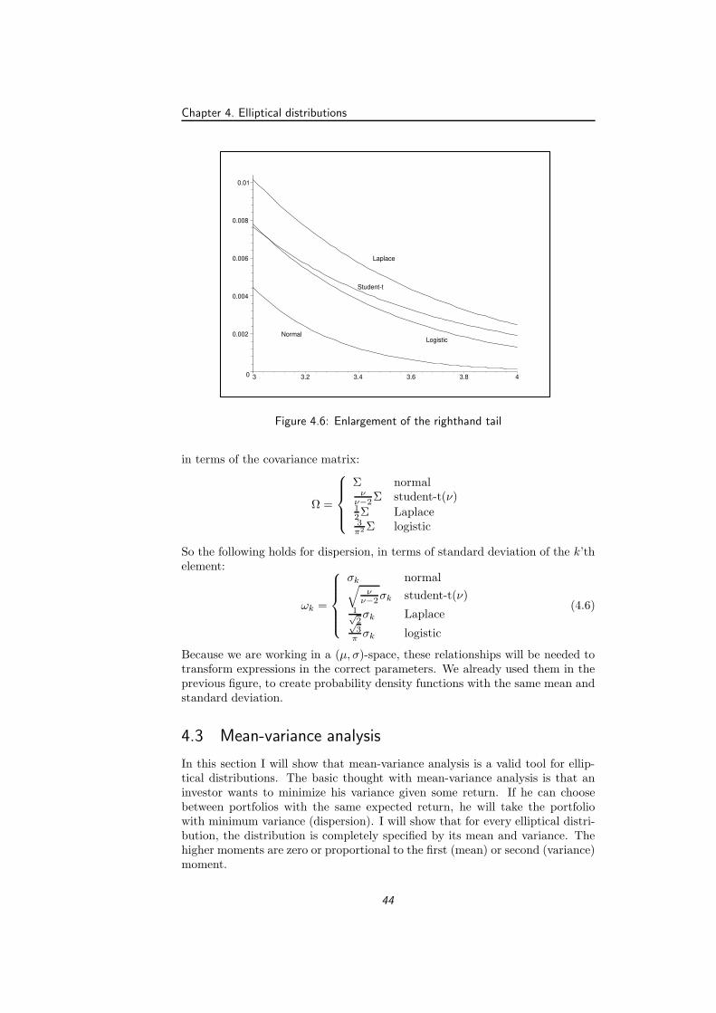
Chapter 4. Elliptical distributions
Laplace
LogisticNormal
Student-t
0
0.002
0.004
0.006
0.008
0.01
3 3.2 3.4 3.6 3.8 4
Figure 4.6: Enlargement of the righthand tail
in terms of the covariance matrix:
Ω =
Σ normalν
ν−2Σ student-t(ν)12Σ Laplace3
π2 Σ logistic
So the following holds for dispersion, in terms of standard deviation of the k’thelement:
ωk =
σk normal√
νν−2σk student-t(ν)
1√2σk Laplace
√3
π σk logistic
(4.6)
Because we are working in a (µ, σ)-space, these relationships will be needed totransform expressions in the correct parameters. We already used them in theprevious figure, to create probability density functions with the same mean andstandard deviation.
4.3 Mean-variance analysis
In this section I will show that mean-variance analysis is a valid tool for ellip-tical distributions. The basic thought with mean-variance analysis is that aninvestor wants to minimize his variance given some return. If he can choosebetween portfolios with the same expected return, he will take the portfoliowith minimum variance (dispersion). I will show that for every elliptical distri-bution, the distribution is completely specified by its mean and variance. Thehigher moments are zero or proportional to the first (mean) or second (variance)moment.
44

4.3. Mean-variance analysis
Suppose that an investor has a portfolio θ of risky assets with portfolioreturn Rp = rT θ = θT r, and that the the vector of asset returns has an ellipticaldistribution: r ∼ En(µ,Ω, ψ), with ψ the characteristic generator as in (4.3),µ the mean and dispersion matrix Ω (I don’t use Σ again on purpose becausethe dispersion matrix doesn’t have to be the covariance matrix). Then theportfolio return is also elliptical distributed, namely Rp ∼ E1(θ
Tµ, θT Ωθ, ψ).Define µp = θTµ the expected portfolio return and ω2 = θT Ωθ the dispersionof the portfolio. The characteristic function of Rp is, by using (4.3),
φp(t) = eitµpψ(1
2tω2t) = eitµpψ(
1
2ω2t2)
The kth central moment about Rp is defined as
E(Rp − µp)k =
∫
(X − µp)kfp(X)dX ≡Mk
with fp(X) the elliptical probability density function of Rp. As we know, thesecond central moment E(Rp − µp)
2 is the variance. With this definition we sethe following:
ψ(1
2ω2t2) = φp(t)e
−itµp ≡ EeitRpe−itµp = Eeit(Rp−µp)
=
∫
eit(X−µp)fp(X)dX =
∫ ∞∑
k=0
(it(X − µp))k
k!fp(X)dX
=
∞∑
k=0
(it)k
k!
∫
(X − µp)kfp(X)dX =
∞∑
k=0
(it)k
k!Mk
= 1 +it
1!M1 +
i2t2
2!M2 +
i3t3
3!M3 + . . .
By noticing that the mth derivative of iktk
k! Mk is
dm
dtm
(
iktk
k!Mk
)
=
0 for k < mm(m−1)(m−2)...(2)(1)imt0
m! Mm = imMm for k = mk(k−1)(k−2)...(k−m+1)iktk−m
k! Mk = iktk−m
(k−m)!Mk for k > m
we see that
dm
dtm
(
ψ(1
2ω2t2)
)∣
∣
∣
∣
t=0
=dm
dtm
( ∞∑
k=0
(it)k
k!Mk
)∣
∣
∣
∣
∣
t=0
= imMm
So the the mth central moment of Rp will be
Mm = i−m dm
dtmψ(
1
2ω2t2)
∣
∣
∣
∣
t=0
The following holds for the mth derivative of ψ( 12ω
2t2), with even m:
dm
dtmψ( 12ω
2t2) =∑m/2
l=0 Cmlψ(m−l)( 1
2ω2t2)ω2(m−l)tm−2l
dm+1
dtm+1ψ( 12ω
2t2) =∑m/2
l=0 Cm+1,lψ(m+1−l)( 1
2ω2t2)ω2(m+1−l)tm+1−2l
45

Chapter 4. Elliptical distributions
where Cml are constants for all m, l. This is easy to prove using induction.Using this result we see that the mth moment can be written as
Mm = Cmψ(m/2)(0)ω2(m/2) = C ′
mωm
Mm+1 = 0for m even
with Cm, C′m constants. We used that, for even m, both i−m and ψ(m/2)(0) are
real constants, and these are included in the constant C ′m.
We see that all odd central moments are zero (this result is not a big surprisebecause every marginal elliptical distribution is, according to (4.5), symmetricaround µ), and all even central moments are proportional to ωm. Therefore,if the density generator is chosen, the distribution of the portfolio return iscompletely characterized by the first two moments, or by mean µp and dispersionω. The first two central moments are
M1 = 0 (so E(Rp) = µp)
M2 = V ar(Rp) = −ψ′(0)ω2
Note that if ψ′(0) = −1, the dispersion ω is equivalent to the standard deviationσp. We have seen this before in the introduction of this chapter.
The result of this proof is that the Telser analysis we did with the normaldistribution, can be easily extended to all elliptical distributions, which we willdo in the next section.
4.4 Telser and elliptically distributed returns
In the previous chapter we have developed a solution for the optimal investmentpolicy with Telser’s approach, where we assumed that asset returns are normallydistributed. In this section we will do the same for elliptically distributed re-turns.
Suppose that asset returns have a multivariate elliptical distribution. So
r ∼ En(µ,Ω, gn)
with expected return vector µ, dispersion matrix Ω and density generator gn(·).We know that the covariance matrix Σ is proportional to Ω and is determined by−ψ′(0)Ω. It follows from the theory (4.4) that the portfolio return is distributedby
Rp = rT θ = θT r ∼ E1(θTµ, θT Ωθ, g1)
If we apply µp = θTµ and ω2p = θT Ωθ this gives
Rp ∼ E1(µp, ω2p, g1)
Note that the portfolios variance is determined by σ2p = −ψ′(0)ω2
p. Then by(4.1) the probability density function of Rp has the following form
fp(x) =c1ωpg1
[
1
2
(
x− µp
ωp
)2]
46

4.4. Telser and elliptically distributed returns
with constant c1 defined (by (4.2)) as
c1 =Γ(1/2)
(2π)1/2
[∫ ∞
0
x1/2−1g1(x)dx
]−1
=1√2
[∫ ∞
0
1√xg1(x)dx
]−1
Telser’s portfolio optimization approach is to maximize the expected returnsubject to the budget constraint that there is a fixed probability of getting intodefault. Remember that the budget constraint is
P (Rp ≤ −C0) ≤ α
Since Rp is elliptically distributed, we can write the probability as
P (Rp ≤ −C0) =
∫ −C0
x=−∞
c1ωpg1
[
1
2
(
x− µp
ωp
)2]
dx
Use the substitution
z =x− µp
ωp⇒ x = zωp + µp ⇒ dx = ωpdz
which gives
P (Rp ≤ −C0) =
∫
−C0−µpωp
z=−∞
c1ωpg1
[
1
2z2
]
ωpdz =
∫
−C0−µpωp
z=−∞c1g1
[
1
2z2
]
dz
Finally define kα as the quantile for which∫ kα
z=−∞c1g1
[
1
2z2
]
dz = α (4.7)
Note that kα only depends on the density generator g(u) and the probabilityα. For example, take the normal distribution. We have seen that g(u) = e−u,c1 = 1√
2π. So for the normal distribution the kα for a probability of α = 0.01 is
the solution of∫ kα
z=−∞
1√2πe−
12z2
dz = 0.01
The solution is k0.01 = −2.33 which is the same as the value for the normalizedquantile kα for the normal distribution defined in the previous chapter. So fromnow on, kα represents the dispersion standardized α-quantile of an ellipticaldistribution. In the table below, some quantiles kα for the previously discussedelliptical distributions are shown.Now we can write for the budget constraint
P (Rp ≤ −C0) ≤ α ⇒ −C0 − µp
ωp≤ kα ⇒ µp ≥ −C0 − kαωp
with kα defined as in (4.7). Because we are working in a (µ, σ)-space, it ispreferable to express the dispersion ωp in terms of standard deviation σp. Using(4.6) for our discussed elliptical distributions, this gives
µp ≥ −C0 − kαωp =
−C0 − kασp normal
−C0 − kα
√
ν−2ν σp student-t(ν)
−C0 − kα1√2σp Laplace
−C0 − kα
√3
π σp logistic
47

Chapter 4. Elliptical distributions
Normal Student-t Student-t Laplace Logistic(ν = 1) (ν = 10)
α = 0.5 0 0 0 0 0α = 0.1 -1.28 -3.08 -1.37 -1.61 -2.20α = 0.01 -2.33 -31.82 -2.76 -3.91 -4.60α = 0.001 -3.09 -318.3 -4.14 -6.21 -6.91α = 0.0001 -3.72 -3183 -5.69 -8.52 -9.21
Table 4.1: The quantiles kα for some elliptical distributions
From now on we will write
µp ≥ −C0 − zασp with zα ≡ kαωp
σp(4.8)
for all elliptical distributions. So for example if returns are distributed accordingto a Laplace distribution, then zα = kα
1√2. The quantile zα can be interpreted
as the standard deviation standardized elliptical quantile, we will refer to zα asthe standardized quantile.
Using this definition, the Telser-optimization problem can be written as
Max
µp ≥ −C0 − zασp
µp 1T θ = C0
µp = µT θσ2
p = θT Σθ
(4.9)
This system is solved in exact the same way as we did for normally distributedreturns, except with the quantile zα instead of kα. So the optimal solution canbe given immediately by looking at the results of the previous chapter. We havefor the case without risk-free asset
θT =1
dΣ−1 ((a1 − bµ)C0 + (cµ− b1)µT )
with
µT =bz2
α + d+√
dz2α(a+ 2b+ c− z2
α)
cz2α − d
C0
If the risk-free asset is added, with rate of return µf , the optimal portfolioallocation changes in
θT ≡
θ1...θN
θf
=
1+µf
s(s+zα)Σ−1 (µf 1 − µ)C0
a+b−(b+c)µf +zαss(s+zα) C0
4.5 Example
In the previous chapter we continued our example of finding the optimal assetallocation with seven securities from the Dutch AEX-index. We assumed thatthe yearly returns were distributed normal, but mentioned that it is very difficult
48

4.5. Example
to find out the real yearly distribution of returns. Main reason was that theyearly time interval is too long to have enough relevant data.
Here we will show what the optimal Telser portfolios are if the yearly returnsare elliptical. We assume the normal, student-t for different degrees of freedom,Laplace and logistic distribution to see what happens with the optimum. Theshortfall probability remains α = 0.0001. The quantiles kα are shown in thenext table.
no risk-free asset with risk-free assetkα zα µT σT µT σT
Normal -3.719 -3.719 0.158 0.311 0.158 0.311Student-t(3) -22.204 -12.819 † † 0.071 0.084Student-t(5) -9.678 -7.496 † † 0.095 0.146Student-t(7) -7.063 -5.970 0.097 0.184 0.110 0.186Student-t(9) -6.010 -5.300 0.116 0.211 0.120 0.211Laplace -8.517 -6.023 0.095 0.182 0.110 0.184Logistic -9.210 -5.078 0.121 0.221 0.124 0.221
Table 4.2: The quantiles kα for some elliptical distributions
The †-sign means that there is no solution of the problem. This is because forthe quantile zα we must have that
|zα| <√a+ 2b+ c = 6.145
to guarantee an optimal solution, which is explained in appendix B. This isclearly not the case when yearly returns are assumed student-t distributed with3 or 5 degrees of freedom. Graphically this can be interpreted that the slope ofthe shortfall line is too steep, and doesn’t have a point of intersection with theefficient frontier, so there is not any point that satisfies the shortfall constraint.In other words, there is no possible asset allocation that will not lose more thanthe invested capital C0 with a probability smaller than α.
Looking at the table we see that all policies are more conservative than whenthe normal distribution is used. This is because the used distributions all havegreater quantiles (at the shortfall probability α) than the normal distribution,or in other words, they have fatter tails: a very bad result is expected to happenmore often. To satisfy the shortfall constraint the investor must decrease hisexpected return, so all means are lower than with normally distributed returns.The optimal allocations θ belonging to the table above are
Normal t(3) t(5) Stud-t(7) Stud-t(9) Laplace logistic-0.088 0.087 0.033 0.093 0.017-0.150 -0.033 -0.069 -0.029 -0.079-0.069 -0.003 -0.023 -0.001 -0.0291.285 † † 0.492 0.736 0.463 0.8060.219 0.036 0.092 0.029 0.108-0.164 0.219 0.101 0.233 0.068-0.033 0.203 0.130 0.211 0.109
Table 4.3: Optimal Telser allocation θ for different yearly distributions
49

Chapter 4. Elliptical distributions
We see that the importance of Heineken and Philips is adjusted downwardswhen more fat-tailed distributions are used. The securities Royal Dutch andUnilever become more important. In a Markowitz context we can say that theoptimum is moving to in the direction of the minimum variance portfolio. If therisk-free asset is added, we have the following optimal Telser allocations:
Normal t(3) t(5) t(7) t(9) Laplace logistic-0.058 -0.016 -0.027 -0.035 -0.040 -0.034 -0.041-0.141 -0.038 -0.066 -0.084 -0.096 -0.084 -0.100-0.062 -0.017 -0.029 -0.037 -0.042 -0.037 -0.0441.258 0.338 0.590 0.751 0.854 0.744 0.8940.203 0.055 0.095 0.121 0.138 0.120 0.144-0.094 -0.025 -0.044 -0.056 -0.064 -0.056 -0.0670.018 0.005 0.009 0.011 0.012 0.011 0.013-0.124 0.699 0.473 0.329 0.238 0.335 0.202
Table 4.4: The optimal Telser allocation θ, with risk-free asset, for different yearlydistributions.
We see that the greater the quantile zα, the more an investor invests at the risk-free rate. So when the shortfall line is becoming steeper, the investor choosesfor more safety and invests more in the risk-free asset.
In a figure, the Telser portfolios with elliptically distributed returns look likethe following. The right figure is a zoomed version of the left figure. The usedshortfall lines are with the normal distribution and the student-t with 3,5,7 and9 degrees of freedom. We also see the efficient frontier(EF), the capital marketline (CML) and the market portfolio (m). Note that there is no optimal solutionif we deal without risk-free asset and assume a student-t(3) or a student-t(5)distribution, which corresponds with the † in the tables before.
Normalt3t5t7t9
EFCML
rf
m
standard deviation
mean
–1
–0.8
–0.6
–0.4
–0.2
0
0.2Normalt3t5t7t9
EF
CML
rf
m
0
0.02
0.04
0.06
0.08
0.1
0.12
0.14
0.16
0.18
0.2
0.1 0.2 0.3 0.4
Figure 4.7: The Telser portfolios with different elliptical distributions
50

4.6. References
4.6 References
Billio, Casarin, Toniolo [2002] Extreme Returns in a Shortfall Risk Framework
Embrechts, McNeil, Straumann [1999] Correlation and Dependence in Risk Ma-nagement: Properties and Pitfalls
Frahm, Junker, Szimayer [2002] Elliptical Copulas: Applicability and Limita-tions
Hodoshima [2001] The Effects on Nonnormality on the Market Model in theClass of Elliptical Distributions
Hult, Lindskog [2001] Multivariate Extremes, Aggregation and Dependance inElliptical Distributions
Ingersoll [1987] Theory of Financial Decision Making
Landsman, Valdez [2002] Tail Conditional Expectations for Elliptical Distribu-tions
Lindskog [2000] Linear Correlation Estimation
Owen, Rabinovitch [1983] ”On the class of Elliptical Distributions and theirapplications to the Theory of Portfolio Choice” The Journal of FinanceVol.38, No.3
Rice [1995] Mathematical Statistics and Data Analysis
Telser [1955] ”Safety-first and Hedging” Review of Economic Studies 23
Valdez, Chernih [2003] Wang’s Capital Allocation Formula for Elliptically-Con-toured Distributions
51


Chapter 5
Value at Risk based optimization
We have seen that the Telser optimization method is not based on standarddeviation as the risk measure. The measure of risk is the probability of gettingin default, P (Rp ≤ −C0). This risk measure is a special case of the world wideused Value at Risk risk measure (VaR). We will discuss the Value at Risk, andportfolio optimization with a VaR constraint, in this chapter.
First the mean-VaR efficient frontier will be derived, both with and withoutrisk-free asset. Section 3 calculates the optimal portfolios with a VaR-constraint,like we did with the Markowitz and Telser framework. The last two sections arefor the example and references.
5.1 VaR efficient frontier
The VaR at level 1 − α of a portfolio (V aRα) is defined by
P (Rp ≤ −V aRα) = α
In words we can say that it is the minimum amount an investor can loose(in dollars) with a confidence interval of 1 − α. The bigger the VaR at someconfidence level, the more risky the portfolio is. So an investor who is extremerisk averse will prefer an extreme low VaR. The figure below shows the graphicalinterpretation of the VaR risk measure.If we take V aRα = C0 and α the shortfall probability, then the VaR defini-tion becomes the shortfall constraint of the previous chapter. So a shortfallconstraint is a special case of a VaR constraint.
Because Value at Risk is our new risk measure, instead of standard deviation,a new efficient frontier can be calculated, just as we did in the mean-standarddeviation framework. The Efficient frontier gives the highest expected return
53

Chapter 5. Value at Risk based optimization
mean
alpha
-VaR 0
VaR
Figure 5.1: Definition of Value at Risk
for some given Value at Risk, or the minimum VaR for a fixed mean. It appearsthat the efficient mean-VaR frontier is the same as the efficient mean-standarddeviation frontier, when returns are elliptically distributed, which we will show.For the calculations in this chapter we will assume returns are elliptically dis-tributed.
When the elliptical assumption is made, the Value at Risk can be written as
P (Rp ≤ −V aRα) = α ⇐⇒ P
(
Rp − µp
ωp≤ −V aRα − µp
ωp
)
= α
⇐⇒ −V aRα − µp
ωp= kα ⇐⇒ V aRα = −µp − kαωp
If we use substitution (4.8), the VaR can be written in terms of mean andstandard deviation:
V aRα = −µp − zασp (5.1)
Remember the negative value of zα. The efficient frontier consists of the pointswhere, for a given mean, the VaR is minimized. It is also defined by the pointswhere, for a given VaR, the mean return is maximized. We will work with thelatter definition, which is in formulas:
Max
V aRα = −µp − zασp
µp µp = µT θσ2
p = θT Σθ1T θ = C0
(5.2)
The first constraint of (5.2) can be transformed to
(V aRα + µp)2 = (−zασp)
2 ⇐⇒ V aR2α + 2V aRαµp + µ2
p − z2ασ
2p = 0
and if we substitute the other constraints we get
V aR2α + 2V aRαµ
T θ + θTµµT θ − z2αθ
T Σθ = 0
⇐⇒ V aR2α + 2V aRαµ
T θ + θT Ψθ = 0
where the matrix Ψ is defined as
Ψ = µµT − z2αΣ
54

5.1. VaR efficient frontier
The maximization problem (5.2) then becomes shorter:
Max
µT θ V aR2α + 2V aRαµ
T θ + θT Ψθ = 01T θ = C0
(5.3)
Ψ is symmetric, because
ΨT = (µµT − z2αΣ)T = (µµT )T − z2
αΣT = µµT − z2αΣ = Ψ
As before, we define the following constants:
a ≡ µT Ψ−1µ
b ≡ µT Ψ−11 = 1T Ψ−1µc ≡ 1T Ψ−11
d ≡ ac− b2
The relationship between the constants a, b, c, d and the familiar constants fromthe previous chapters a, b, c, d can be easily derived. The following holds for theinverse covariance matrix
Σ−1 = Σ−1ΨΨ−1 = Σ−1(µµT − z2αΣ)Ψ−1 = Σ−1µµT Ψ−1 − z2
αΨ−1
Using this expression for Σ−1 we have
a = µT Σ−1µ = µT Σ−1µµT Ψ−1µ− z2αµ
T Ψ−1µ = aa− z2αa = a(a− z2
α)
b = µT Σ−11 = µT Σ−1µµT Ψ−11 − z2αµ
T Ψ−11 = ab− z2αb = b(a− z2
α)
c = 1T Σ−11 = 1T Σ−1µµT Ψ−11 − z2α1T Ψ−11 = bb− z2
αc
We solve this set to get the desired expressions, and get
a = aa−z2
α
b = ba−z2
α
c =cz2
α−dz2
α(a−z2α)
d = ac− b2 = −dz2
α(a−z2α)
(5.4)
Later on we will use this results to compare the derived results with previousfindings.
We solve the problem (5.3) using the Lagrange method. This gives thefollowing set of equations
µ+ 2λ1V aRαµ+ 2λ1Ψθ + λ21 = 0 (a)V aR2
α + 2V aRαµT θ + θT Ψθ = 0 (b)
1T θ = C0 (c)
Solving equation (a) for θ gives, with λ3 = 1−2λ1
and λ4 = − λ2
2λ1:
θ = (λ3 − V aRα)Ψ−1µ+ λ4Ψ−11 (5.5)
Using this θ in (c), we get an expression for λ4:
1T θ = (λ3 − V aRα)b+ λ4c = C0
55

Chapter 5. Value at Risk based optimization
⇐⇒ λ4 =C0 + bV aRα − λ3b
c
The calculation of λ3 follows from (b). After many calculations, which areshown in appendix A, we get
λ23 =
1
d
(
V aR2α(d− c) − 2C0bV aRα − C2
0
)
So
λ3 = ±√
1
d
(
V aR2α(d− c) − 2C0bV aRα − C2
0
)
≡ ±√W
Since we now have values for λ3 and λ4, we calculate θ using (5.5), which gives
θ = (±√W − V aRα)Ψ−1µ+
1
c(C0 + V aRαb∓
√W )Ψ−11
So the desired expression for the portfolio mean, as a function of the Value atRisk, is
µp = µT θ = (±√W − V aRα)a+
1
c(C0 + V aRαb∓
√W )b
=d
c
(
±√W − V aRα +
b
dC0
)
(5.6)
Using the minus sign in this expression gives the mean-VaR efficient frontier.To compare this frontier with the mean-standard deviation efficient frontier, wefirst invert the function (write V aRα as a function of µp). In (5.6), we isolate√W , take squares on both sides and solve the arisen quadratic function for
V aRα. This gives:
V aRα = −µp +
√
1
d
(
(d− c)µ2p + 2bC0µp − aC2
0
)
The second step is to substitute the constants a, b, c, d for constants a, b, c, d.We use substitution (5.4) for this, and get
V aRα = −µp − zα
√
1
d
(
cµ2p − 2bC0µp + aC2
0
)
(5.7)
The last step is to transform this equation to the mean-standard deviationframework. We use the substitution (5.1) for V aRα and get
−µp − zασp = −µp − zα
√
1
d
(
cµ2p − 2bC0µp + aC2
0
)
where zα is assumed to be negative. So the mean-VaR efficient frontier in amean-standard deviation framework is given by
σp =
√
1
d
(
cµ2p − 2bC0µp + aC2
0
)
(5.8)
which we recognize as the mean-variance efficient frontier! So our conclusioncan be that minimizing the variance is the same as minimizing the Value atRisk, when returns are elliptically distributed.
56

5.1. VaR efficient frontier
mean
standard deviation
mean
value at risk
Figure 5.2: The efficient frontier in mean-standard deviation and mean-VaR frame-work
The two frontiers are shown in the following two graphs, the left figure isthe efficient frontier in a mean-standard deviation framework, the right figureis the same efficient frontier in a mean-VaR framework.
Because the mean-standard deviation efficient frontier and the mean-VaRefficient frontier are the same, the allocation at the frontier is still given (interms of µp) by (2.3).
We have seen analytically what the relationship is between the efficient fron-tiers in mean-standard deviation space and mean-VaR space. This relationshipcan also be shown in a figure, as shown below. The slope of the shortfall lines inthe left graph depends on the (elliptical) distribution of returns and the short-fall probability α, but is a fixed constant. The values p, q, r in the left graphare similar to the values p, q, r in the right graph, so the cross-lines in the rightgraph have slope 1.
value at risk
mean
rqp
-r
-q
-p
mean
standard deviation
Figure 5.3: Graphical relationship of the efficient frontier in mean-st.dev. andmean-VaR framework.
57

Chapter 5. Value at Risk based optimization
5.2 Adding the risk-free asset
In the mean-standard deviation framework, the efficient frontier changes intothe capital market line when a risk-free asset is introduced. An investor thenwill invest in a combination of the market portfolio and the risk-free asset.Remember that the CML is given by
µp = sσp + C0µf with s =√
cµ2f − 2bµf + a (5.9)
The constant s is the slope of the CML. The representation of the CML in themean-VaR framework can be derived using (5.1) as an expression for σp andsubstituting this in (5.9). This gives
µp = sσp + C0µf = s
(−V aRα − µp
zα
)
+ C0µf
which results in the CML for the mean-VaR framework:
µp =−s
zα + sV aRα +
zαµf
zα + sC0 (5.10)
The figure below shows the capital market line in the two settings. The con-struction lines show how the two lines are related to each other. The point of
value at risk
mean
rqp
-r
-q
-p
mean
standard deviation
Figure 5.4: Graphical relationship of the CML in mean-st.dev. and mean-VaRframework.
tangency between the CML and the efficient frontier is the market portfolio.We have seen in the Markowitz chapter that the mean return in the marketportfolio is µm =
a−bµf
b−cµfC0. To see which Value at Risk belongs to the market
portfolio we equalize µm with (5.10) and get
a− bµf
b− cµfC0 =
−szα + s
V aRα +zαµf
zα + sC0
58

5.3. Optimal portfolios
which results in
V aRm =bµf − a− zαs
b− cµfC0
where we used the substitution s2 = cµ2f − 2bµf + a. So (V aRm, µm) is the
market portfolio in the mean-VaR framework. The allocation θm remains theallocation calculated in the mean-standard deviation market portfolio section.
5.3 Optimal portfolios
Like we did in the mean-standard deviation framework, we can derive differentoptimal portfolios in the mean-VaR framework. An investor can choose to investin the minimum Value at Risk portfolio, which is the portfolio that minimizesthe VaR. The minimum VaR portfolio differs from the minimum variance port-folio, which can be seen by comparing the efficient frontiers in both frameworks.Another interesting portfolio is the tangency portfolio in the mean-VaR frame-work. This is the portfolio that maximizes the ratio mean/VaR, so it gives theportfolio with maximal return per unity VaR. Looking in a Telser context, wecan calculate the optimal Telser portfolio, which is the portfolio that maximizesthe expected return, while satisfying a Value at Risk constraint. We will lookat this in a framework with and without a risk-free asset.
5.3.1 Minimum Value at Risk portfolio
The minimum Value at Risk portfolio is the portfolio that minimizes the Valueat Risk. Because we have derived formula (5.7) as the efficient frontier, we onlyhave to set the derivative of this function to zero and solve it for µp. We get
∂V aRα
∂µp= −1 − zα(cµp − bC0)
d√
1d (cµ2
p − 2bC0µp + aC20 )
= 0 (5.11)
Solving this for µp results in the minimum VaR expected return
µmvr =
(
b
c+
d
c√
cz2α − d
)
C0
The corresponding Value at Risk is calculated by using (5.7):
V aRmvr = −µmvr − zα
√
1
d(cµ2
mvr − 2bC0µmvr + aC20 )
=
(
−bc
+1
c
√
cz2α − d
)
C0
The minimum VaR standard deviation is
σmvr =
√
1
d(cµ2
mvr − 2bC0µmvr + aC20 ) =
−zα√
cz2α − d
C0
The asset allocation θ at the minimum Value at Risk portfolio is calculated byusing (2.3), the allocation on the efficient frontier, which results in
θmvr =1
c√
cz2α − d
Σ−1(
(√
cz2α − d− b)1 + cµ
)
C0
59

Chapter 5. Value at Risk based optimization
The minimum value at risk portfolio is shown in the following figure, which isin the mean-VaR framework.
mvr
mean
value at risk
Figure 5.5: The minimum VaR portfolio
5.3.2 Tangency VaR portfolio
The tangency VaR portfolio is the portfolio where the line through the originis tangent to the mean-VaR efficient frontier. It represents the portfolio withmaximum ratio mean/VaR, so with maximum value for mean per unit VaR.
At the tangency VaR portfolio, the slope of the tangency line must be thesame as the slope of the efficient frontier. So
∆V aRtvr
∆µtvr=∂V aRα
∂µp
∣
∣
∣
∣
µp=µtvr
Using formula (5.7), we get the following equation
−µtvr − zα
√
1d (cµ2
tvr − 2bC0µtvr + aC20 ) − 0
µtvr − 0=
−1− zα(cµp − bC0)
d√
1d (cµ2
p − 2bC0µp + aC20 )
∣
∣
∣
∣
∣
∣
µp=µtvr
The solution of this equation is
µtvr =a
bC0
We see that this is the same result as the tangency portfolio in a mean-standarddeviation framework! So µtvr = µtg. Looking better, it is clear that this resultis quite logic. Because
Maximizeµp
V aRα= Maximize
µp
−µp − zασp= Minimize
−µp − zασp
µp
60

5.3. Optimal portfolios
= Minimize−zασp
µp= Maximize
µp
σp
the maximization of the tangency line in the mean-VaR framework and themean-standard deviation framework gives the same result. The correspondingVaR is
V aRtg = −µtg − zασtg = −√a
b(√a+ zα)C0
and the allocation θtg is the same as the allocation in the mean-standard devi-ation tangency portfolio.
The portfolio looks like the following in a figure.
tg
mean
value at risk
Figure 5.6: The minimum VaR portfolio
5.3.3 Telser
We defined the optimal Telser portfolio as the portfolio that maximizes expectedreturn subject to a shortfall constraint. Because the shortfall constraint is a spe-cial case of a Value at Risk constraint, we redefine the definition of the optimalTelser portfolio. From now on, the optimal Telser portfolio is the portfolio thatmaximizes the expected return while satisfying a Value at Risk constraint. Ifwe need the ”old version” of the Telser portfolio, we take V aR = C0 in thedefinition. So the Telser problem looks like
Max
V aRα ≤ V aRc
µp 1T θ = C0
µp = µT θ
(5.12)
where V aRc is the maximum allowed Value at Risk of the portfolio. When weassume that returns are distributed elliptically, the first constraint of (5.12) canbe rewritten as (use expression (5.1) for the VaR):
V aRα ≤ V aRc ⇐⇒ V aRc ≥ V aRα = −µp − zασp
⇐⇒ µp ≥ −V aRc − zασp
61

Chapter 5. Value at Risk based optimization
So the optimization problem transforms to
Max
µp ≥ −V aRc − zασp
µp 1T θ = C0
µp = µT θσ2
p = θT Σθ
(5.13)
If we take the maximum allowed Value at Risk V aRc equal to the startingcapital, so V aRc = C0, we exactly get the ”old” formulation as described in theSafety First chapter. The corresponding figures for problem (5.13) look like thefollowing, where the optimum lies in area A, and the optimum is found at themaximum expected return, so at point opt. The left graph is in mean-standarddeviation space, the right graph in mean-VaR space. These two graphs clearly
opt
A
standard deviation
-VaR(c)
mean
value at risk
A
mean
VaR(c)
opt
Figure 5.7: The optimal Telser portfolio
show why it is useful to work with the mean-VaR efficient frontier. It is becausethe Value at Risk constraint becomes a vertical line, which is much easier towork with.
The optimal point is calculated by using the mean-VaR efficient frontier (5.7)with V aRα = V aRc, which gives
V aRc = −µp − zα
√
1
d
(
cµ2p − 2bC0µp + aC2
0
)
Solving this for µp results in
µopt =bz2
αC0 + dV aRc − zα
√
d((a− z2α)C2
0 + 2bV aRcC0 + cV aR2c)
cz2α − d
The corresponding standard deviation is
σopt =
(−V aRc − µopt
zα
)
=zα(bC0 + cV aRc) −
√
d((a− z2α)C2
0 + 2bV aRcC0 + cV aR2c)
d− cz2α
62

5.3. Optimal portfolios
and the Value at Risk equals V aRc. The optimal asset allocation θopt is foundby using the fact that the optimal portfolio lies on the efficient frontier, so wecan use formula (2.3) we derived in the Markowitz chapter:
θopt =1
dΣ−1 ((cµ− b1)µopt + (a1 − bµ)C0)
5.3.4 Telser with risk-free asset
If we add a risk-free asset, the efficient frontier changes into the CML. Theoptimal Telser portfolio with risk-free asset is the portfolio where maximumreturn is gained, while satisfying the VaR-constraint. In the figures below, weare looking for the highest return in the area A. This is at point opt, the pointof intersection between the CML and the VaR constraint line.
A
standard deviation
-VaR(c)
mean
opt
value at riskVaR(c)
A
mean
opt
Figure 5.8: The optimal Telser portfolio with risk-free asset
For the calculation of this point of intersection we use the mean-VaR frame-work, because the VaR constraint line is vertical. Remember the CML is givenby (5.10). The point of intersection is at the point where V aRα = V aRc, so
µopt =−sV aRc + C0zαµf
zα + s
The corresponding standard deviation is
σopt =µopt + V aRc
−zα= −C0µf + V aRc
zα + s
and the Value at Risk is V aRc. For calculating the optimal asset allocationwith risk-free asset, we do the same as we did before in the Markowitz andTelser chapters. The optimal allocation consists of a combination the marketportfolio and the risk-free asset. Suppose a fraction Θm is invested in the marketportfolio and a fraction Θf in the risk-free asset. The two fractions sum toone. Because the returns on the risk-free asset have no standard deviation, theportfolio standard deviation of the optimal portfolio is given by
σopt =√
Θ2mσ
2m + Θ2
f · 0 = Θmσm
63

Chapter 5. Value at Risk based optimization
where σm is the standard deviation in the market portfolio, derived in theMarkowitz chapter. So the fraction invested in this market portfolio is
Θm =σopt
σm=
−C0µf+V aRc
zα+ss
b−cµfC0
=(C0µf + V aRc)(cµf − b)
s(zα + s)C0
So the fraction invested in the risk-free asset is
Θf = 1 − Θm =(a− bµf + szα)C0 + V aRc(b− cµf )
s(zα + s)C0
where we used that s =√
cµ2f − 2bµf + a. So the optimal allocation with risk-
free asset becomes
θopt ≡
θ1...θN
θf
=
Θmθm
ΘfC0
=
V aRc+µf C0
s(s+zα) Σ−1 (µf 1 − µ)
(a−bµf +szα)C0+V aRc(b−cµf )s(zα+s)
5.4 Example
We continue the example of seven securities of the Dutch AEX-index. In theElliptical Distributions chapter, the optimal Telser portfolio was calculated us-ing the shortfall constraint. This shortfall constraint was a yearly probabilityof getting in default, and that was the reason why we transformed the dailyreturns into yearly returns. In this chapter we switched to a VaR constraint.But in contrast to the shortfall constraint, the VaR is given for a much shorterperiod, mostly one day. So the daily returns can be used again. The probabilityα is also adjusted. The confidence level for the one day VaR that Rabobank isusing at the moment is 97,5%, so
α = 0.025
We will not assume that the daily returns have a normal distribution. Becausewe have 3609 observations of the daily returns from the 1st of January 1990till the 31st of October 2003, we can estimate the distributions of the sevensecurities. We use the quantile-quantile(QQ)-plot for this.
A QQ-plot is useful for comparing a set of data with different distributionfunctions. The quantiles of the date are plotted against the quantiles of some(elliptical) distribution functions. The data are sort and standardized for eachdistribution using the mean and standard deviation and these are comparedwith the quantiles kα, where α is taken from 3609 values in the interval [0,1].The best fitting of the distribution of returns for each asset is the plot that isclosest to the 45 degrees line, because both quantiles are close to each otherthere. This results in the QQ-plots at the next pages.
In every plot the normal distribution is shown. It is clear that for none of thesecurities the normal distribution is a good approximation of the distributionfunction. Also two or three other elliptical distributions (student-t, Laplace,logistic) are shown, these are the two or three that are closest to the 45 degreesline.
64

5.4. Example
(OVHYLHU
-8
-6
-4
-2
0
2
4
6
8
-8 -6 -4 -2 0 2 4 6 8
norm
t7
t5
t6
)RUWLV
-10
-8
-6
-4
-2
0
2
4
6
8
10
-10 -8 -6 -4 -2 0 2 4 6 8 10
norm
Lapl
t5
t7
*HWURQLFV
-20
-15
-10
-5
0
5
10
15
20
-16 -12 -8 -4 0 4 8 12 16
normt5t4
t3
+HLQHNHQ
-10
-8
-6
-4
-2
0
2
4
6
8
10
-10 -8 -6 -4 -2 0 2 4 6 8 10
t6t7
Lapl
norm
Figure 5.9: QQ-plots of Elsevier, Fortis, Getronics and Heineken.
65

Chapter 5. Value at Risk based optimization
3KLOLSV
-8
-6
-4
-2
0
2
4
6
8
-8 -6 -4 -2 0 2 4 6 8
t6
t7
Lapl
norm
5R\DO'XWFK
-10
-8
-6
-4
-2
0
2
4
6
8
10
-10 -8 -6 -4 -2 0 2 4 6 8 10
t6t7
log
norm
8QLOHYHU
-8
-6
-4
-2
0
2
4
6
8
-8 -6 -4 -2 0 2 4 6 8
normt7
t6
Figure 5.10: QQ-plots of Philips, Royal Dutch and Unilever.
66

5.4. Example
With these plots we can estimate the distributions of the returns. Notethat we are only interested in the left tail distribution, because for the VaRconstraint we need the 0.025 quantile. By looking at the QQ-plots the followingdistributions of the left tail can be estimated:
Elsevier student-t(6)/student-t(7)Fortis student-t(7)/Laplace
Getronics student-t(3)Heineken student-t(6)/student-t(7)
Philips student-t(6)/LaplaceRoyal Dutch student-t(7)
Unilever student-t(7)/student-t(6)
Table 5.1: Estimated left tail distribution of returns
Notice that Getronics has a difficult elliptical match. The fluctuation in thelast years was very high, so the tails are very fat,and there is not an ellipticaldistribution that really fits. The estimated student-t with 3 parameters of free-dom is the closest. But all the others are quite close to each other. Especiallythe student-t distribution with 6 or 7 degrees of freedom fits for the other sixsecurities. Because a choice for the portfolio distribution has to be made, Ichoose the student-t distribution with 6 degrees of freedom as the distributionof portfolio returns.
The quantile kα of the student-t(6) distribution for α = 0.025 is
k0.025 = −2.447
so the standardized quantile zα is
z0.025 = k0.025
√
ν − 2
ν= −2.447
√
6− 2
6= −1.998
Note that this value doesn’t differ much from the quantile if returns wouldbe expected to be distributed normally, because then we would have z0.025 =k0.025 = −1.960. If we move further to the tail of the distribution, so α decreases,the difference between the quantiles grows. This is shown in the table below,where the quantiles for different elliptical distributions and different values forα have been calculated.
α = 0.025 α = 0.01 α = 0.0001kα zα kα zα kα zα
Normal -1.96 -1.96 -2.33 -2.33 -3.72 -3.72Student-t(3) -3.18 -1.84 -4.54 -2.62 -22.20 -12.82Student-t(4) -2.78 -1.96 -3.75 -2.65 -13.03 -9.22Student-t(6) -2.45 -2.00 -3.14 -2.57 -8.02 -6.55Student-t(8) -2.31 -2.00 -2.90 -2.51 -6.44 -5.58Student-t(10) -2.23 -1.99 -2.76 -2.47 -5.69 -5.09Laplace -3.00 -2.12 -3.91 -2.77 -8.52 -6.02Logistic -3.66 -2.02 -4.60 -2.53 -9.21 -5.08
Table 5.2: The quantiles for some elliptical distributions at different α
67

Chapter 5. Value at Risk based optimization
It is clear that only for extreme low α it matters what the distribution of returnslooks like. If a VaR-confidence level of 97,5% is used, like we do, the results forstudent-t distributed returns with 4 up to and including 10 degrees of freedomare very close to the normally distributed returns. The same holds for logisticdistributed returns.
The mean-VaR efficient frontier is given by
V aRα = −µp − zα
√
1
d
(
cµ2p − 2bC0µp + aC2
0
)
= −µp + 1.998√
2882.2µ2p − 1.891µp + 0.435× 10⁻³
The minimum Value at Risk portfolio has the following coordinates:
µmvr =
(
b
c+
d
c√
cz2α − d
)
C0 = 0.330× 10⁻³
V aRmvr =
(
−bc
+1
c
√
cz2α − d
)
C0 = 0.0219
σmvr =−zα
√
cz2α − d
C0 = 0.0112
The asset allocation θmvr at the minimum Value at Risk portfolio is
θmvr =1
c√
cz2α − d
Σ−1(
(√
cz2α − d− b)1 + cµ
)
C0 =
0.130−0.0040.0130.296−0.0090.3140.261
which is a quite diversified portfolio.Suppose the investor has a Value at Risk limit of 10%, so V aRc = 0.1. This
means that the probability that he loses more than 10 percent of his money isless then α = 0.025. Then the optimal Telser mean, standard deviation andallocation are
µT =bz2
αC0 + dV aRc − zα
√
d((a− z2α)C2
0 + 2bV aRcC0 + cV aR2c)
cz2α − d
= 1.249×10⁻³
σT =
(−V aRc − µT
zα
)
= 0.0507
θT =1
dΣ−1 ((cµ− b1)µT + (a1 − bµ)C0) =
−0.537−0.451−0.2383.3220.690−1.147−0.639
68

5.4. Example
Realize that this value for the VaR is quite high, because the optimal portfolioinvests very much in Heineken and goes short in five other securities to generatethe amount invested in Heineken. If the investor is more risk averse, so the VaRlimit is lower, the following happens. We take V aRc = 0.05.
µT = 0.753× 10⁻³, σT = 0.0254, θT =
−0.177−0.210−0.1021.6900.313−0.359−0.154
And for V aRc = 0.025 we have
µT = 0.443× 10⁻³, σT = 0.0127, θT =
0.048−0.059−0.0180.6670.0760.1350.150
If the risk-free asset is added, with rate of return µf = 0.157 × 10⁻³, theefficient frontier changes into the CML, which is in mean-VaR space
µp =−s
zα + sV aRα +
zαµf
zα + sC0 = 0.0122V aRα + 0.159× 10⁻³
The Value at Risk at the market portfolio, for which we have calculated thatµm = 0.580× 10⁻³, is
V aRm =bµf − a− zαs
b− cµfC0 = 0.0344
The values for the optimal Telser portfolio with risk-free asset are calculatedwith
µT =−sV aRc + C0zαµf
zα + s, σT = −C0µf + V aRc
zα + s
θT =
V aRc+µf C0
s(s+zα) Σ−1 (µf 1 − µ)
(a−bµf +szα)C0+V aRc(b−cµf )s(zα+s)
The results that these formulas give for different values of the VaR limit aregiven in the following table.
We see that the more risk averse (the lower the VaR) the investor is, the lowerthe expected return. The standard deviation gets also lower and the amountborrowed at the risk-free rate becomes less. When V aRc = 0.025, the investoreven lends at the risk-free rate. In the figure below, this is shown by the factthat this optimum lies on the left side of the market portfolio. We also see theminimum VaR portfolio(mvr), market portfolio(m), the efficient frontier(EF),capital market line(CML) and the three Value at Risk constraints.
69

Chapter 5. Value at Risk based optimization
V aRc = 0.1 V aRc = 0.05 V aRc = 0.025µT 1.382× 10⁻³ 0.770× 10⁻³ 0.465× 10⁻³
σT 0.0507 0.0254 0.0127-0.150 -0.075 -0.038-0.364 -0.182 -0.091-0.159 -0.080 -0.040
θT 3.241 1.623 0.8140.524 0.262 0.132-0.242 -0.121 -0.0610.046 0.023 0.012
θrf -1.895 -0.450 0.273
Table 5.3: Optimal Telser portfolio results with risk-free asset
5.5 References
Artzner, Delbaen, Eber, Heath [1998] Coherent Measures of Risk
Carroll, Perry, Yang, Ho [2001] ”A New Approach to Component VaR” Journalof Risk 3
Di Clemente [2003] The Empirical Value-at-Risk/Expected Return Frontier: aUseful Tool of Market Risk Managing
Frei, McNeil [2002] VaR and Expected Shortfall in Portfolios of Dependent CreditRisks: Conceptual and Practical Insights
De Giorgi [2002] A Note on Portfolio Selection under Various Risk Measure
mvr
CML
m
VaR=0.025
VaR=0.10
VaR=0.05
EF
rf
mean
value at risk
0
0.0002
0.0004
0.0006
0.0008
0.001
0.0012
0.0014
0.02 0.04 0.06 0.08 0.1 0.12
Figure 5.11: Optimal Portfolios with VaR constraint.
70

5.5. References
Huisman, Koedijk, Pownall [1999] Asset Allocation in a Value-at-Risk Frame-work
Hurlimann [2001] An alternative Approach to Portfolio Selection
Lucas [1998] Nut, Gebruik, en Beperkingen van Value-at-Risk voor Risicoman-agement
Lucas [1997] A Note on Optimal Estimation from a Risk Management Perspec-tive under Possibly Mis-specified Tail Behavior
Tasche [2000] Risk Contributions and Performance Measurement
71


Chapter 6
Maximizing the performance
measures EVA and RAROC
We have studied optimization problems with different objective functions. Inthe Markowitz framework, the objective was to maximize the utility functionu = E(Rp) − 1
2γvar(Rp). This function appeared to be a convex curve inthe mean-standard deviation space. In the Telser framework the objective wasto maximize the expected return E(Rp) subject to some shortfall or Value atRisk constraints. In this chapter we will discuss some models, based on theTelser criterion, but with other objective functions. These objective functionsare based on the so called Economic Value Added (EVA) and the Risk AdjustedReturn On Capital (RAROC).
6.1 EVA and RAROC
EVA The Economic Value Added is defined as follows
EVA = expected portfolio return − cost of capital
The higher the EVA, the better the performance of the investor. The expectedportfolio return is given by E(Rp). But because there are costs for keepingcapital, the expected return is corrected for this costs. The cost of capitalconsists of two parameters. It is the cost of capital rate rcap multiplied bythe amount of capital. It is not generally agreed how the amount of capital isdefined. There are two main streams: some say the amount of capital is theinvestors equity capital C0 (or the allocated capital), some say it is the Valueat Risk V aR (or the consumed capital). Note that the EVA is an absolute
73

Chapter 6. Maximizing the performance measures EVA and RAROC
performance measure, because the total cost of capital is subtracted. So it is anominal amount, not a percentage.
RAROC There are numerous different definitions of the RAROC performancemeasure. The Risk Adjusted Return On Capital we will use in this thesis isdefined as
RAROC =expected portfolio return
amount of capital
The higher the RAROC, the better the investors performance. The maximumRAROC gives the highest expected return, relative to the amount of capital, soRAROC is a relative risk measure. Again, the amount of capital can be definedas the allocated capital C0, or the consumed capital V aR.
The following table shows the performance measures described above:
allocated capital consumed capital
EVA E(Rp) − rcapC0 E(Rp) − rcapV aRα
RAROCE(Rp)
C0
E(Rp)V aRα
Table 6.1: Overview of the performance measures EVA and RAROC
The next sections will solve new models based on the EVA and RAROC per-formance measures.
6.2 New Telser models
We have seen four new performance measures in the table above. These fourmeasures can all be implemented in the Telser model with Value at Risk con-straint, by setting them as the objective function. We solve the four obtainednew Telser models in the next four sections. The fifth section compares someoptimal solution with each other.
6.2.1 EVA with allocated capital
Using the EVA with allocated capital as the objective function, we get thefollowing optimization problem
Max
E(Rp) = µp = µT θE(Rp) − rcapC0 P (Rp ≤ −V aRc) ≤ α
1T θ = C0
Because rcapC0 is a constant, and rewriting the shortfall constraint, this problemis the same as
Max
µp = µT θµp V aRα ≤ V aRc
1T θ = C0
74

6.2. New Telser models
which we recognize as the Telser problem of the previous chapter. So the solutionis given by
µopt = µT =bz2
αC0 + dV aRc − zα
√
d((a− z2α)C2
0 + 2bV aRcC0 + cV aR2c)
cz2α − d
(6.1)with corresponding standard deviation
σopt = σT =zα(bC0 + cV aRc) −
√
d((a− z2α)C2
0 + 2bV aRcC0 + cV aR2c)
d− cz2α
(6.2)and the Value at Risk equals V aRc. The optimal asset allocation θopt is
θopt = θT =1
dΣ−1 ((cµ− b1)µT + (a1 − bµ)C0)
In the mean-VaR space, the graphical reproduction looks like the following.
mean
VaR(c)
opt
value at risk
A
Figure 6.1: Optimal ”EVA with allocated capital” portfolio
6.2.2 EVA with consumed capital
If the consumed capital is used instead of the allocated capital, in the EVAobjective function, the optimization problem becomes
Max
E(Rp) = µp = µT θE(Rp) − rcapV aRα V aRα ≤ V aRc
1T θ = C0
The objective function, E(Rp) − rcapV aRα ≡ u is a line in the mean-VaRframework. The line is given by
µp = u+ rcapV aRα
and maximizing the EVA means maximizing u, or moving the line as high aspossible in the feasible area A, while keeping the slope coefficient rcap constant.
75

Chapter 6. Maximizing the performance measures EVA and RAROC
mean
VaR(c)
opt
value at risk
A
Figure 6.2: Moving the EVA-line with large rcap
We call this line the EVA-line. The feasible area A is the area between the short-fall line and the efficient frontier. See the figure below for a possible outcome.
Moving the EVA-line as high as possible gives the optimal portfolio opt. Aswe can see in the figure, the optimal portfolio differs from the Telser point. Inthis optimum, the slope of the EVA-line (rcap) equals the slope of the efficientfrontier. But this optimal portfolio strongly depends on the value for rcap, theslope of the EVA-line.
If the slope of the EVA-line is much smaller (which means that rcap is muchsmaller), we can get the figure below.
mean
opt
VaR(c)value at risk
A
Figure 6.3: Moving the EVA-line with small rcap
Notice the difference from the situation before. Because the feasible areaA is bounded by the shortfall constraint line, the highest EVA-line intersectsthe efficient frontier at the Telser point, and the optimum is not at the point of
76

6.2. New Telser models
tangency of the efficient frontier and the EVA-line.So, the optimal allocation is either at the point where the slope of the EVA-
line and the efficient frontier are the same (see the first figure, situation 1) orat the Telser point (second figure, situation 2), and it depends on the EVA-line slope, rcap, in which situation we are. The turning point between thetwo situations is where the EVA-line is tangent to the efficient frontier, and thetangency point is exactly at the Telser point, which is shown in the figure below.
mean
opt
VaR(c)value at risk
A
Figure 6.4: The tangency point is the Telser point
We will calculate at which value for rcap this turning point is reached. There-fore we must equalize the slope of the efficient frontier at the Telser point andthe slope of the EVA-line, or
∂µp
∂V aRα
∣
∣
∣
∣
µp=µT
= rcap ⇐⇒ ∂V aRα
∂µp
∣
∣
∣
∣
µp=µT
=1
rcap(6.3)
Remember that the efficient frontier (in mean-VaR space) is given by
V aRα = −µp − zα
√
1
d
(
cµ2p − 2bC0µp + aC2
0
)
So the derivative of V aRα with respect to µp is given by
∂V aRα
∂µp= −1− zα(cµp − bC0)
d√
1d
(
cµ2p − 2bC0µp + aC2
0
)
=−dσp − zα(cµp − bC0)
dσp
Using this derivative in (6.3) and solving for rcap, we get
rcap =dσT
−dσT − zα(cµT − bC0)≡ r∗cap
where µT and σT are the mean and standard deviation at the Telser point,given by (6.1) and (6.2) respectively. So we have situation 1 if rcap > r∗cap, andsituation 2 if rcap ≤ r∗cap.
77

Chapter 6. Maximizing the performance measures EVA and RAROC
We will derive the optimal values. The optimum in situation 2 is the Telserportfolio, which is already calculated. Let us calculate the optimum in situation1. In the optimum (see the first figure), the (inverse of the) slope of the efficientfrontier equals (the inverse of) rcap, for which rcap > r∗cap. So
∂V aRα
∂µp=
1
rcap
−1− zα(cµp − bC0)
d√
1d
(
cµ2p − 2bC0µp + aC2
0
)
=1
rcap(6.4)
Solving this for µp gives (after isolating, taking squares and solving the quadraticproblem),
µopt =
(
b+d√
cK2 − d
)
1
cC0
where K is a constant defined by K =zαrcap
rcap+1 . Notice that K < 0. This result
can be achieved also by noticing that (6.4) can be written as
−1 − 1
rcap− zα(cµp − bC0)
d√
1d
(
cµ2p − 2bC0µp + aC2
0
)
= 0
If we divide this byrcap+1
rcap, we get
−1−zαrcap
rcap+1 (cµp − bC0)
d√
1d
(
cµ2p − 2bC0µp + aC2
0
)
= −1 − K(cµp − bC0)
d√
1d
(
cµ2p − 2bC0µp + aC2
0
)
= 0
This is the same expression as formula (5.11) in the minimum Value at Risksection, with the difference that zα is replaced by K. So the solution of (6.4)is given by the solution µmvr of (5.11), with zα replaced by K. This gives thesame optimal mean as derived above.
The corresponding σopt is
σopt =
√
1
d
(
cµ2opt − 2bC0µopt + aC2
0
)
=−K√cK2 − d
C0
and the Value at Risk equals
V aRα = −µopt − zασopt =
(
−bc
+czαK − d
c√cK2 − d
)
C0
which concludes the optimal portfolio in situation 1.Summarized we can say the following for the optimal µp when the objective
is to maximize the EVA with consumed capital:
µopt =
(
b+ d√cK2−d
)
1cC0 if rcap > r∗cap
µT if rcap ≤ r∗cap
with K =zαrcap
rcap + 1
where µT , the Telser mean, is given by (6.1). The corresponding optimal allo-cation θopt is on the efficient frontier:
θopt =1
dΣ−1 ((cµ− b1)µopt + (a1 − bµ)C0)
78

6.2. New Telser models
6.2.3 RAROC with allocated capital
We leave the EVA-based objective function and start looking at the RAROC-based objective. First we look at the case where we deal with allocated capital.The RAROC maximizing optimization problem becomes
Max
E(Rp) = µT θE(Rp)
C0P (Rp ≤ −V aRc) ≤ α
1T θ = C0
Because C0 is a constant, and rewriting the shortfall constraint, this problem isthe same as
Max
µp = µT θµp V aRα ≤ V aRc
1T θ = C0
which is identical to the Telser problem and the EVA optimization problem withallocated capital. So the solutions of this problem are the same as the solutionsin the EVA allocated capital section.
6.2.4 RAROC with consumed capital
The RAROC optimization problem when we are dealing with consumed capitalis
Max
E(Rp) = µp = µT θE(Rp)V aRα
V aRα ≤ V aRc
1T θ = C0
The objective functionµp
V aRα≡ u can be written as the RAROC-line
µp = uV aRα
so maximizing the RAROC corresponds with finding the maximum slope u ofthe line through the origin, which still has overlap with the feasible area A.
opt
VaR(c)
A
mean
value at risk
Figure 6.5: Maximizing the slope of the RAROC-line
79

Chapter 6. Maximizing the performance measures EVA and RAROC
We see that the optimum is the tangency point in the mean-VaR framework,as defined in the previous chapter. Remember that this is the same tangencypoint as in the mean-standard deviation framework. This means that
µopt =a
bC0, σopt =
√a
bC0, V aRα = −
√a
b(√a+ zα)C0
Note that there can occur a problem if the tangency value for V aRα, −√
ab (
√a+
zα)C0, is on the right side of the shortfall line V aRc. Then the tangency V aRα
is not in the feasible area A. Thus we have to reduce the slope of the RAROC-line till it touches the feasible area. Then the optimum moves to the Telserpoint, as can be seen in the figure below. So we can summarize it as follows:
A
VaR(c)
tg
T
Figure 6.6: The situation if the tangency Value at Risk exceeds V aRc
µopt =
µT if V aRc < −√
ab (
√a+ zα)C0
µtg if V aRc ≥ −√
ab (
√a+ zα)C0
and again the corresponding optimal allocation θopt is on the efficient frontier:
θopt =1
dΣ−1 ((cµ− b1)µopt + (a1 − bµ)C0)
6.2.5 Comparison EVA-RAROC
A simple comparison can be made between the EVA and RAROC performancemeasures. We already have seen that the EVA is a nominal amount and theRAROC is a percentage. But what is the relationship between the optima?
If allocated capital is used, the optimal portfolios are the same because theyboth are the optimal Telser portfolio. It is more interesting to look at the casewhere consumed capital is used. We discuss four situations.
Situation 1 Suppose that
rcap ≤ r∗cap and V aRc ≤ −√a
b(√a+ zα)C0.
Then in both situations the Telser portfolio is optimal, so the optimum withthe EVA performance measure is identical to the optimum with the RAROCperformance measure. We write µEV A
opt = µRAROCopt .
80

6.2. New Telser models
Situation 2 This changes when the following situation appears:
rcap ≤ r∗cap and V aRc > −√a
b(√a+ zα)C0.
Then the optimal EVA portfolio remains the Telser optimum, but the RAROCmaximizing portfolio changes into the tangency portfolio. So in this case wehave that µEV A
opt > µRAROCopt .
Situation 3 The third possible situation is that
rcap > r∗cap and V aRc ≤ −√a
b(√a+ zα)C0.
In this case, the EVA maximizing portfolio is smaller than the Telser portfolio,which is the optimal RAROC portfolio, so µEV A
opt < µRAROCopt .
Situation 4 The last possibility is that the following occurs:
rcap > r∗cap and V aRc > −√a
b(√a+ zα)C0.
Now we have that
µEV Aopt =
(
b+d√
cK2 − d
)
1
cC0, µRAROC
opt =a
bC0
We calculate for which value of rcap these two optima are the same. Then
(
b+d√
cK2 − d
)
1
cC0 =
a
bC0
which results in the easy expression
K = −√a
Because K =zαrcap
rcap+1 , we see after a little calculation that
rcap =−√
a
zα +√a
So if the cost of capital rate equals this value, we have that µEV Aopt = µRAROC
opt .If the value for rcap is smaller, the EVA line gets a smaller slope, so the optimalEVA mean moves to the right. In the other way, if rcap is greater the optimummoves to the left. Concluding we can say the following for this fourth situation:
µEV Aopt < µRAROC
opt if rcap >−√
azα+
√a
µEV Aopt = µRAROC
opt if rcap = −√a
zα+√
a
µEV Aopt < µRAROC
opt if rcap >−√
azα+
√a
Remember that in any case we must have in this situation that rcap > r∗cap.
81

Chapter 6. Maximizing the performance measures EVA and RAROC
6.3 Models with risk-free asset
Like with most models, we can add the risk-free asset with constant rate ofreturn µf . Remember that the efficient frontier changes in the capital marketline, which is given by
µp =−s
zα + sV aRα +
zαµf
zα + sC0 with s =
√
cµ2f − 2bµf + a
when we are working in the mean-VaR space.
6.3.1 EVA
For maximizing the EVA, when dealing with allocated capital, we can handle thesame as in the previous section without risk-free asset. Because the allocatedcapital is a constant, the EVA-maximization problem
Max
E(Rp) = µp = µT θ + µfθf
E(Rp) − rcapC0 P (Rp ≤ −V aRc) ≤ α1T θ + θf = C0
can be written as
Max
µp = µT θ + µfθf
µp V aRα ≤ V aRc
1T θ + θf = C0
which solution is exactly the optimal Telser portfolio, as calculated in the pre-vious chapter. See also the left figure below for a graphical view of the problemand solution. The optimal values are
µopt =−sV aRc + C0zαµf
zα + s, σopt = −C0µf + V aRc
zα + s, V aRα = V aRc
R(f)
CML
mean
A
value at risk
opt
VaR(c)
R(f)
mean
CML
A
value at riskVaR(c)
Figure 6.7: EVA maximization solutions with risk-free asset
If the EVA performance measure deals with consumed capital, the problemchanges. The solution of the problem
Max
E(Rp) = µp = µT θ + µfθf
E(Rp) − rcapV aRα V aRα ≤ V aRc
1T θ + θf = C0
82

6.3. Models with risk-free asset
again is finding the maximum u in the EVA-line
µp = u+ rcapV aRα
with slope rcap. But because the efficient frontier is the CML (with slope −szα+s
in the mean-VaR space), we see in the right figure above that there are threepossibilities. If the slope of the EVA-line is greater then the CML slope, thehighest EVA-line starts at the risk-free point, which will be the optimum. If theslope of the CML is greater then the EVA-line slope, the EVA-line will move uptill it reaches the Telser portfolio, which wil be the optimum. If the two slopesare identical, every point on the CML is optimal, as long as it stays on the leftside of the VaR-constraint line.
It is clear that this situation of maximizing the Economic Value Added withconsumed capital and risk-free asset is not really useful, because the optimalpoint is either at the left extremum (investing everything in the risk-free asset)or it is the Telser portfolio. Thus when there exists a risk-free asset, the EVAperformance measure is not a suitable objective function.
6.3.2 RAROC
For the RAROC maximization problem with allocated capital and risk-free asset,we get the same result as with the EVA performance measure with allocatedcapital. Because the maximization of E(Rp)/C0 (with C0 a constant) is thesame as the maximization of E(Rp), finding the optimum is exactly the Telserproblem with risk-free asset. So the optimal point is the point in the feasiblearea with maximum expected return, which is the point of intersection of theCML and the VaR-constraint line. This is shown in the left figure below.
A
mean
value at risk
opt
VaR(c)
CML
R(f) optA
mean
value at riskVaR(c)
CML
R(f)
Figure 6.8: RAROC maximization solutions with risk-free asset
If we deal with consumed capital, the solution is different. We know thatmaximizing the ratio E(Rp)/V aRα means finding the greatest slope of the linethrough the origin (we call it the RAROC-line), which still lies in the feasiblearea. But, as the right figure below shows, we can rotate the RAROC-line untilit reaches the risk-free point. Notice that it does not stop at the tangency point,as was the case in the situation without risk-free asset. Because the Value atRisk goes to zero when moving to the risk-free point, the RAROC ratio tends
83

Chapter 6. Maximizing the performance measures EVA and RAROC
to infinity. So when the risk-free asset is involved, the RAROC with consumedcapital can go to infinity is everything is invested in the risk-free asset, so thisperformance measure is not realistic.
Summarized we can say that, if the risk-free asset is added, both the EVAand RAROC performance measure give the Telser portfolio (with risk-free asset)as the optimal portfolio if we deal with allocated capital. But if the consumedcapital is used for the performance measures, the optimal solutions are eitherthe risk-free portfolio or the Telser portfolio.
6.4 Example
We continue our example. Suppose that the portfolio return is distributedaccording to a student-t(6) distribution, like we did in the previous chapter,so the standardized quantile, where the Value-at-Risk confidence level is taken97,5%, is
z0.025 = −1.998
The cost of capital rate within Rabobank is 10% per year. Because we areworking in a daily context, we take
rcap = 1 − (0.90)(1/250) = 0.421× 10⁻³
In this example we allow a maximum Value at Risk of 0.05, so
V aRc = 0.05
The EVA allocated capital problem gives the Telser portfolio of the previouschapter (with V aRc = 0.05) as the optimum. These optimal values are
µT = 0.753× 10⁻³, σT = 0.0254, θT =
−0.177−0.210−0.1021.6900.313−0.359−0.154
and the optimum is given by point s in the figure. If we deal with consumedcapital, the optimum changes. We calculate r∗cap to see which formula gives theoptimum.
r∗cap =dσT
−dσT − zα(cµT − bC0)= 0.0105 > rcap
Because rcap < r∗cap, also in this case the optimum is the Telser portfolio withresults as above. Again this is point s in the figure.
If the objective is to maximize the RAROC, the result when using the al-located capital is again the Telser portfolio (s in the figure). If the consumedcapital is used, we have to determine the tangency VaR. This is
V aRtg = −√a
b(√a+ zα)C0 = 0.0259 < V aRc
84

6.5. References
So because V aRc > −√
ab (
√a+ zα)C0, the optimal portfolio is given by
µopt = abC0 = 0.596× 10⁻³
σopt =√
ab C0 = 0.0132
V aRα = −√
ab (
√a+ zα)C0 = 0.0259
θopt = 1dΣ−1 ((cµ− b1)µopt + (a1 − bµ)C0) =
0.036−0.067−0.0220.7230.0890.1080.134
This is point q in the figure. In the figure we see that the slope of the EVA-lineis quite small. We can calculate what the rcap has to be if we want the optimalEVA portfolio with consumed capital to be the same as when the consumedRAROC is used. The we must have that
rcap =−√
a
zα +√a
= 0.0177
at a daily basis, which means a value of
rcap = 1− (1 − 0.0177)250 = 0.989
per year. So if the cost of capital rate is 98.9%, the two optima are equal toeach other. This is an extraordinary high value which will not happen in reality.
If the risk-free asset is added, the solutions for the objectives that deal withconsumed capital become either the portfolio that consists only of the risk-freeasset or the Telser portfolio. In the EVA case, the Telser portfolio is the result,while in the RAROC case it results in the risk-free portfolio (which gives infiniteRAROC). The optimal portfolios with allocated capital are simply the Telserportfolios with risk-free asset, which we have seen in the previous chapter. Thesolution is given by
µT = 0.770× 10⁻³, σT = 0.0254, θT =
−0.075−0.182−0.0801.6230.262−0.1210.023−0.450
In the figure, this portfolio is represented by point r. Also shown in the figureare the efficient frontier(EF), capital market line(CML), Value at Risk line, EVAline, and the RAROC line.
6.5 References
Baud, Frachot, Igigabel, Martineau, Roncalli [1999] An Analysis Framework forBank Capital Allocation
85

Chapter 6. Maximizing the performance measures EVA and RAROC
EVA-line
EFrf
CML
q
RAROC-line
VaR=0.05
sr
mean
value at risk0
0.0002
0.0004
0.0006
0.0008
0.01 0.02 0.03 0.04 0.05 0.06
Figure 6.9: Optimal EVA and RAROC portfolios.
Bralver, Kuritzkes [19??] ”Risk Adjusted Performance Measurement in theTrading Room” Journal of Applied Corporate Finance
Jameson [2001] ”Between Raroc and a Hard Place” ERisk.com
Punjabi [1998] ”Many Happy Returns” Risk Magazine June
Rabobank Nederland [2003] Economic Capital from a Conceptual Point of View.Internal Memo.
Smithson [2001] ”Allocating and Optimising Capital” Risk Magazine June
Wilson [1992] ”Raroc Remodelled” Risk Magazine September
86

Chapter 7
Modeling uncertainty of input
parameters
This chapter deals with the role of parameter uncertainty in the models we havedescribed. It shows what happens if the chosen parameters µ and Σ are notcertain. This is because in reality, it is very difficult to estimate the correctvalues of these parameters and these correct values change every day.
7.1 Overview
There are several techniques proposed in the literature to handle this parameteruncertainty. Basic thought is to reduce the sensitivity of the optimal portfoliosto input uncertainty. In other words, if the input parameters µ and Σ change asmall amount, the optimal portfolio should not change much.
Frost and Savarino propose to constrain the portfolio weights, so one singleasset doesn’t become too important for the portfolio. Chopra et al. proposesto use a James-Stein Estimator for means, while Black and Litterman suggestBayesian estimation of means and covariances. Jorion researches the Bayes-Stein estimators. There are also sample-based and scenario-based approaches,as described in papers of Michaud and Ziemba et al. All these methods reducethe sensitivity of the portfolio allocation to the input parameters, but do notprovide any hard guarantees on the portfolio performance.
A proposal to model parameter uncertainty in this thesis is as follows.It arose after many discussions with statisticians and econometricians withinRabobank. We define a probability distribution function for the uncertain pa-rameters µ and Σ, and include this in the optimization problem. The objectivefunction, which is the expected return in the Telser framework, now has to deal
87

Chapter 7. Modeling uncertainty of input parameters
not only with uncertainty of the returns, which is given by µ and σ, but alsowith uncertainty in these last two parameters. So the uncertainty parametersare uncertain, and a ’second layer’ uncertainty is created. This must result in anew simultaneous distribution of portfolio returns, which depends asset returns,means and covariances. There are some difficulties with this method. First thedistribution functions of µ and Σ are very difficult to determine. Second, ifthese distribution functions are determined, the new simultaneous distributionfunction is even more difficult to find. After this, the optimization has to beexecuted with this new simultaneous distribution function which probably willnot be elliptical, which seems to be a hopeless task. Besides this, this methodstill doesn’t provide any hard guarantees on the portfolio performance.
That is why, throughout this thesis, I will discuss another approach. The in-put parameters µ and σ are expected to lie within a confidence interval, and theoptimization problem will be solved for the worst case scenario. The confidenceinterval is called the uncertainty set. This means that, for example if we workwith a Value at Risk constraint, in none of the possible input situations theportfolio VaR will exceed the VaR limit. So the investor is guaranteed a certainportfolio return, because the worst-case situation is optimized. In the literaturethis robust optimization is considered by for instance Ben-Tal and Nerirovski,and Goldfarb and Iyengar.
7.2 Uncertainty sets
Suppose an investor doesn’t know the exact values for the mean return vectorand covariance matrix, but that he knows a certain interval the parameters arelying in. The intervals are bounded by a lower bound and an upper bound, sowe can write
µLi ≤ µi ≤ µU
i ∀iσL
ij ≤ σij ≤ σUij ∀i, j
Instead of using the above notation we will use, with µ0i = (µL
i + µUi )/2, βi =
(µUi − µL
i )/2, σ0ij = (σL
ij + σUij)/2 and δij = (σU
ij − σLij)/2, the following:
µ0i − βi ≤ µi ≤ µ0
i + βi ∀i
σ0ij − δij ≤ σij ≤ σ0
ij + δij ∀i, jSo the uncertainty sets of the mean return Sm and the covariance Sv can bewritten as
Sm = µ : µ0 − β ≤ µ ≤ µ0 + β, β ≥ 0 (7.1)
Sv = Σ : Σ0 − ∆ ≤ Σ ≤ Σ0 + ∆,∆ ≥ 0 (7.2)
These are the uncertainty sets we will use in this chapter.
7.3 Second order cone programming
The optimal values for the Markowitz and Telser portfolios (without parameteruncertainty) in the previous chapters were explicit expressions, obtained byusing either Lagrange’s method or the Kuhn-Tucker conditions. So far, it is
88

7.3. Second order cone programming
not possible to find an explicit expression for the optimal values when we areconsidering the worst case outcomes for the uncertain parameters. Instead, wewill be able to reduce the problems to a second order cone problem (SOCP),which can be solved fast using a computer. A SOCP is an optimization problemof the following form:
Min
fTx ‖Aix+ bi‖ ≤ cTi x+ di, i = 1, . . . , N
(7.3)
where ‖ · ‖ is the standard Euclidean norm, so ‖u‖ =√uTu for a vector u.
Vectors f , x and c are n-dimensional, while x is the decision variable. Thereare N constraints.
Second order cone programming is a problem class that lies between linearprogramming and semidefinite programming (SDP). SOCPs can be solved farmore efficiently than SDPs, so if a SDP can be written as a SOCP, this ispreferred.
The constraints in (7.3) are called second order cone constraints. This hasthe following reason. Note that the standard second order cone of dimension kis defined as
Ck =
(
ut
)
with ‖u‖ ≤ t (7.4)
where u is a (k − 1)-dimensional vector and t is a scalar. For example, in thethree dimensional space (k = 3) we have that the formula for the standardsecond order cone is
z ≥√
x2 + y2
which has the following graph:
2
4
6
8
10
12
14
–10
10
y–10–8–6–4–2
46810x
Figure 7.1: The standard second order cone
Now suppose that we have the following set of points
(
Ai
cTi
)
x+
(
bidi
)
with Ai a (k−1)×n-matrix, ci and bi vectors of n respectively (k−1) dimensions,and di a scalar. When this set of points lies in the standard cone of dimensionk, the following must hold
(
Ai
cTi
)
x+
(
bidi
)
∈ Ck ⇐⇒(
Aix+ bicTi x+ di
)
∈ Ck
89

Chapter 7. Modeling uncertainty of input parameters
And because of (7.4) we must have
‖Aix+ bi‖ ≤ cTi x+ di
which is the second order cone constraint in (7.3).A SOCP includes the family of Linear Programs, which can be seen by
taking Ai the zero-matrix and bi the zero-vector, so the constraint transformsto the linear constraint 0 ≤ cTi x+ di. SOCPs include many more optimizationproblems, like quadratic programs, problems with hyperbolic constraints andproblems involving sums and maxima of norms, which is shown in Lobo et al.(1998).
For solving SOCPs, there are some interior point methods available. Thismethods are implemented in computer software like SEDUMI and SDPT3. Wewill use the SEDUMI package, which is an optimizer that uses the power ofMATLAB, to solve the problems we will face in the next sections. For makingthe implementation of SEDUMI in MATLAB easier we use the program Yalmip.
7.4 Portfolio optimization and SOCP
In this thesis we have optimized the Markowitz portfolio and the Telser port-folio with a Value at Risk constraint. We used the techniques of Lagrange anKuhn-Tucker to get an explicit expression for the optimal portfolio’s. But theseproblems can also be written as a SOCP.
7.4.1 Markowitz
Remember that the Markowitz optimization problem is
Max
µT θ − 12γθ
T Σθ 1T θ = C0
with positive risk-aversion parameter γ. We can rewrite this as
Min
θT Σθ − 2γµ
T θ 1T θ = C0
and by noticing the following (we add and subtract the same constant andperform some other operations)
θT Σθ − 2
γµT θ
=(
Σ1/2θ)T (
Σ1/2θ)
− 1
γθT Σ1/2Σ−1/2µ− 1
γµT Σ−1/2Σ1/2θ
+
(
1
γΣ−1/2µ
)T (1
γΣ−1/2µ
)
−(
1
γΣ−1/2µ
)T (1
γΣ−1/2µ
)
=
(
Σ1/2θ − 1
γΣ−1/2µ
)T (
Σ1/2θ − 1
γΣ−1/2µ
)
− 1
γ2µT Σ−1µ
= ‖Σ1/2θ − 1
γΣ−1/2µ‖2 − a
γ2
90

7.5. Portfolio optimization with uncertainty
we can write the optimization problem as
Min
‖Σ1/2θ − 1γ Σ−1/2µ‖2 − a
γ2 1T θ = C0
Because, in a SOCP, we must have a linear objective function, we add a variablet to achieve this, which gives an extra constraint. The result is
Min
t ‖Σ1/2θ − 1γ Σ−1/2µ‖ ≤ t
0 = 1T θ − C0
which is the SOCP of the form (7.3) belonging to the optimal Markowitz port-folio.
7.4.2 Telser
We do the same with the Telser optimization problem. We have shown beforethat the Telser problem with elliptically distributed returns, maximum Valueat Risk V aRc (which implies the constraint P (Rp ≤ −V aR) ≤ α) and corre-sponding (negative) quantile zα can be written as
Max
µT θ µT θ ≥ −V aRc − zα
√θT Σθ
1T θ = C0
which is easy to transform in a SOCP. If we use that√θT Σθ = ‖Σ1/2θ‖ we get
Min
−µT θ ‖Σ1/2θ‖ ≤ 1−zα
µT θ + 1−zα
V aRc
0 = 1T θ − C0
7.5 Portfolio optimization with uncertainty
Let’s look at the optimization problem with the uncertainty sets for µ andΣ, as described in (7.1) and (7.2) respectively. We have explained that theuncertainty will be handled by evaluating the worst case scenario. But what isthe worst case expected return and covariance? If no short sales are allowed (ie.no borrowing), it is clear that the worst case expected return is the minimalexpected return, which is the lower bound µ − β. But in this thesis we allowshort sales (borrowing), so this is not sufficient. If an investor goes short inan asset, the worst case expected return for that asset is the highest possiblereturn, because this costs the investor the most money. Then we have to dealwith the highest expected return for this asset, or the upper bound µi +βi. Forthe covariances we can use the same reasoning. Concluding we can say that itdepends on the investment policy if we have to use the upper or lower boundfor both the expected return and covariance matrix.
7.5.1 Markowitz
The Markowitz portfolio optimization problem in the worst case scenario is
Maxθ
minµ,Σ
[
µT θ − 12γθ
T Σθ]
1T θ = C0
91

Chapter 7. Modeling uncertainty of input parameters
where γ is the parameter of risk aversion. Because γ > 0 we can write theproblem as
Maxθ
minµ
[
µT θ]
− 12γmaxΣ
[
θT Σθ]
1T θ = C0
(7.5)
First, we find an expression for the minimum expected return:
minµ[µT θ] = minµ
∑
i
µiθi =∑
i:θi<0
(µ0i + βi)θi +
∑
i:θi≥0
(µ0i − βi)θi
=∑
i
µ0i θi +
∑
i:θi<0
βiθi −∑
i:θi≥0
βiθi =∑
i
(
µ0i θi − βi|θi|
)
= (µ0)T θ − βT |θ| (7.6)
We can do the same with the maximum variance. This gives
maxΣ
[
θT Σθ]
= maxΣ
∑
i,j
σijθiθj
=∑
i,j:θiθj<0
(σ0ij − δij)θiθj +
∑
i,j:θiθj≥0
(σ0ij + δij)θiθj
=∑
i,j
σ0ijθiθj +
∑
i,j
δij |θiθj | =∑
i,j
σ0ijθiθj +
∑
i,j
δij |θi||θj |
= θT Σ0θ + |θ|T ∆|θ| (7.7)
With this results the optimization problem (7.5) becomes a bit simpler:
Maxθ
(µ0)T θ − βT |θ| − 12γθ
T Σ0θ − 12γ|θ|T ∆|θ| 1T θ = C0
This problem is a SOCP, so it can be solved in an efficient way. To show this, wehave to do some work. We add two variables ρ and τ in the objective function.We get
Maxθ,ρ,τ
1T θ = C0
(µ0)T θ − βT |θ| − 12γρ− 1
2γτ ρ ≥ θT Σ0θτ ≥ |θ|T ∆|θ|
Note that for any positive definite A, vector x and positive scalar y we can write
xTAx ≤ y ⇔ 4xTAx ≤ 4y ⇔ 4xTAx− 2y + y2 + 1 ≤ 2y + y2 + 1
⇔ 4xTA1/2A1/2x+ (1 − y)2 ≤ (1 + y)2 ⇔∥
∥
∥
∥
(
2A1/2x1 − y
)∥
∥
∥
∥
≤ (1 + y)
Using this, we can rewrite two constraints and get the following
Maxθ,ρ,τ
1T θ = C0
(µ0)T θ − βT |θ| − 12γ(ρ+ τ)
∥
∥
∥
∥
(
2(Σ0)1/2θ1 − ρ
)∥
∥
∥
∥
≤ 1 + ρ∥
∥
∥
∥
(
2∆1/2|θ|1 − τ
)∥
∥
∥
∥
≤ 1 + τ
92

7.5. Portfolio optimization with uncertainty
which is almost a SOCP as in (7.3). The only problem is the absolute valuesign of θ. We can replace |θ| by a new n-dimensional vector η and addingthe constraints ηi ≥ θi and ηi ≥ −θi for all i, which guarantees ηi ≥ |θi|.Another way of dealing with the absolute value is replacing θ respectively |θ| byθ = θ+ − θ− respectively |θ| = θ+ + θ− and adding the positivity constraintsθ+i , θ
−i ≥ 0 for all i. We use the first transformation, which results in the
following SOCP:
Minθ,ρ,τ,η
1T θ = C0∥
∥
∥
∥
(
2(Σ0)1/2θ1 − ρ
)∥
∥
∥
∥
≤ 1 + ρ
−(µ0)T θ + βT η + 12γ(ρ+ τ)
∥
∥
∥
∥
(
2∆1/2η1 − τ
)∥
∥
∥
∥
≤ 1 + τ
ηi ≥ θi for all iηi ≥ −θi for all i
This is the formulation of the Markowitz optimization problem as a SOCP. Asstated before, this can be solves using a computer. The MATLAB program Iuse, robustmarkowitz.m, is in appendix C.
7.5.2 Telser
In the worst case scenario, the Telser optimization problem with VaR constraintbecomes
Maxθ
minµ
[
µT θ]
1T θ = C0
maxµ,Σ [P (Rp ≤ −V aRc)] ≤ α
Since for the robust mean we have
minµ
[
µT θ]
= (µ0)T θ − βT |θ|
and for the VaR constraint
maxµ,Σ [P (Rp ≤ −V aRc)] ≤ α ⇐⇒ maxµ,Σ−V aRc − µT θ√
θT Σθ≤ zα
⇔ −V aRc −minµµT θ
maxΣ
√θT Σθ
≤ zα ⇐⇒ −minµµT θ− zαmaxΣ
√θT Σθ ≤ V aRc
which can be transformed into
−(µ0)T θ + βT |θ| − zα
√
θT Σ0θ + |θ|T ∆|θ| ≤ V aRc
⇐⇒ −zα
∥
∥
∥
∥
(
‖(Σ0)1/2θ‖‖∆1/2|θ|‖
)∥
∥
∥
∥
≤ (µ0)T θ − βT |θ| + V aRc
So we have the following optimization problem:
Maxθ
1T θ = C0
(µ0)T θ − βT |θ| −zα
∥
∥
∥
∥
(
‖(Σ0)12 θ‖
‖∆1/2|θ|‖
)∥
∥
∥
∥
≤ (µ0)T θ − βT |θ| + V aRc
93

Chapter 7. Modeling uncertainty of input parameters
To make it a SOCP we introduce new variables ρ and τ , so the problem becomes
Maxθ,ρ,τ
1T θ = C0
(µ0)T θ − βT |θ| −zα
∥
∥
∥
∥
(
ρτ
)∥
∥
∥
∥
≤ (µ0)T θ − βT |θ| + V aRc
‖(Σ0)1/2θ‖ ≤ ρ
‖∆1/2|θ|‖ ≤ τ
The last step is the introduction of the new variable η to remove the absolutevalue parameters. This gives us the SOCP
Minθ,ρ,τ,η
1T θ = C0
−zα
∥
∥
∥
∥
(
ρτ
)∥
∥
∥
∥
≤ (µ0)T θ − βT η + V aRc
−(µ0)T θ + βT η ‖(Σ0)1/2θ‖ ≤ ρ
‖∆1/2η‖ ≤ τηi ≥ θi for all iηi ≥ −θi for all i
This SOCP can be solved using the MATLAB program robusttelser.m inappendix C.
7.6 A more realistic approach
As we will see in the example, the approach described above is a very conser-vative approach. Main reason for this is the definition of worst case portfoliovariance ((σ2
p)wc) we used. When deriving this worst case portfolio variance(7.7), we took for every element σij of the covariance matrix the worst caseelement. In formulas:
(σ2p)wc = (θT Σθ)wc =
∑
i,j
σwcij θiθj
This means the worst case covariance matrix Σwc can be represented as
Σwc =
σwc11 σwc
12 · · · σwc1n
σwc21
. . ....
...σwc
n1 · · · σwcnn
But is it likely that this special case will occur? No is the answer. This isbecause this particular worst case covariance matrix is composed of covarianceswhich do not belong to each other. The covariances are taken out of differentcovariance matrices, and so the correlation between the covariances is disturbed.
That is why it is more logic to compose the worst case portfolio variance asfollows:
(σ2p)wc = (θT Σθ)wc =
∑
i,j
σijθiθj
wc
94

7.6. A more realistic approach
So the worst case covariance matrix is given by
Σwc =
σ11 σ12 · · · σ1n
σ21. . .
......σn1 · · · σnn
wc
Suppose an investor knows (for example from studying the past) that there arem possible covariance matrices Σ1,Σ2 . . . ,Σm. Then the worst case covariancematrix in the first meaning is the matrix that consists of all the worst caseelements σk
ij for all i, j = 1, . . . , n and k = 1, . . . ,m. The worst case covariance
matrix in the second meaning is the worst case matrix Σk for all k = 1, . . . , n.In this new situation we do not model parameter uncertainty in µ. This is
because according to the experts within Rabobank the uncertainty in the covari-ances is much more important than the uncertainty in the means. Furthermorethe uncertainty in µ is very difficult to measure.
7.6.1 Markowitz
This new way of modelling uncertainty can be applied to the optimal Markowitzportfolio. Assume there are m possible covariance matrices Σ1,Σ2 . . . ,Σm andthat the mean vector is ’certain’. Then the robust Markowitz problem
Maxθ
minµ,Σ
[
µT θ − 12γθ
T Σθ]
1T θ = C0
can be transformed to
Maxθ
µT θ − 12γmaxk[θT Σkθ] 1T θ = C0
⇐⇒ Maxθ
µT θ − 12γρ 1T θ = C0
ρ ≥ maxk[θT Σkθ]
⇐⇒ Maxθ
µT θ − 12γρ 1T θ = C0
ρ ≥ θT Σkθ for all k
⇐⇒ Minθ
−µT θ + 12γρ 1T θ = C0
∥
∥
∥
∥
(
2(Σk)1/2θ1 − ρ
)∥
∥
∥
∥
≤ 1 + ρ for all k
This is a SOCP. Note that this expression is simpler than the previously cre-ated version of the uncertain Markowitz problem. The corresponding MATLABprogram robustmarkowitz2.m is in appendix C.
7.6.2 Telser
For the Telser problem with VaR constraint we can do the same. The robustVaR constraint is
maxΣ [P (Rp ≤ −V aRc)] ≤ α ⇐⇒ maxk−V aRc − µT θ√
θT Σkθ≤ zα
⇐⇒ −V aRc − µT θ
maxk
√θT Σkθ
≤ zα ⇐⇒ −zαmaxk
√θT Σkθ ≤ µT θ + V aRc
95

Chapter 7. Modeling uncertainty of input parameters
⇐⇒ −zα
√θT Σkθ ≤ µT θ + V aRc for all k
⇐⇒ −zα‖(Σk)1/2θ‖ ≤ µT θ + V aRc for all k
So the robust Telser optimization problem becomes
Minθ
−µT θ 1T θ = C0
−zα‖(Σk)1/2θ‖ ≤ µT θ + V aRc for all k
This is the another version of the uncertain Telser optimization problem. TheMATLAB program for solving this has the name robusttelser2.m and can befound in appendix C.
7.7 Example
The programs of this chapter will be implemented in our example. First we willfind the uncertainty sets of µ and Σ. When this is done, we run the MATLABprograms of appendix C to see what the results are.
7.7.1 Uncertainty sets
An important question is how to determine the uncertainty sets. Tutuncuand Koenig [2002] propose two methods. The first method is a bootstrappingmethod, where time series are bootstrapped from the available data. The secondmethod is a moving window method. A window of 60 days is taken and withinthis window the means and covariances are determined. The window is movedback in time to get lower and upper bounds for the means and covariances.
I will use a variant of the last method. Also a window of 60 days is taken,and means and covariances are calculated for this window. Then the window ismoved 60 days back in time to calculate the second mean vector and covariancematrix. This is done 60 times (because we have 3609 observations), so at the endwe have 60 possible mean vectors and 60 possible covariance matrices. Noticethat the first 9 observations (this are observations in the year 1990!) are ignored.From these data the uncertainty sets are determined.
The data give the following lower and upper bounds for means and covari-ances (see the tables).
×10−3 µLi µU
i
Elsevier -4.79 4.86Fortis -6.37 8.35
Getronics -32.79 29.21Heineken -3.28 6.26
Philips -12.00 7.59Royal Dutch -3.19 4.71
Unilever -4.88 4.71
Table 7.1: Lower and upper bounds for means
With this lower and upper bounds it is easy to determine the vectors µ0 and β,and the matrices Σ0 and ∆. With the means for example, we use
µ0i =
µLi + µU
i
2∀i and βi =
µUi − µL
i
2∀i
96

7.7. Example
×10−3 Els For Get Hei Phi RDu UniElsevier 0.057 -0.009 -0.017 -0.049 -0.045 -0.065 -0.035
1.721 1.300 2.109 0.448 1.060 0.549 0.528Fortis -0.009 0.065 -0.171 -0.029 -0.219 -0.006 0.000
1.300 2.508 2.185 0.532 1.830 1.340 0.994Getronics -0.017 -0.171 0.059 -0.175 -0.048 -0.222 -0.430
2.109 2.185 29.715 0.707 1.977 0.990 1.127Heineken -0.049 -0.029 -0.175 0.039 -0.166 -0.030 -0.005
0.448 0.532 0.707 1.024 0.525 0.420 0.352Philips -0.045 -0.219 -0.048 -0.166 0.081 -0.065 -0.556
1.060 1.830 1.977 0.525 3.049 1.242 0.838Royal Dutch -0.065 -0.006 -0.222 -0.030 -0.065 0.029 -0.022
0.549 1.340 0.990 0.420 1.242 1.156 0.758Unilever -0.035 0.000 -0.430 -0.005 -0.556 -0.022 0.031
0.528 0.994 1.127 0.352 0.838 0.758 0.986
Table 7.2: Lower and upper bounds for covariances
to determine the wanted vectors. This gives the following vectors:
µ0 =
0.0360.988−1.7931.493−2.2040.760−0.088
× 10−3 β =
4.8267.35831.0024.7719.7913.9524.796
× 10−3
For covariances the same properties hold. So the matrices Σ0 and ∆ are:
Σ0 =
0.889 0.645 1.046 0.200 0.508 0.242 0.2470.645 1.287 1.007 0.252 0.806 0.667 0.4971.046 1.007 14.887 0.266 0.965 0.384 0.3480.200 0.252 0.266 0.532 0.180 0.195 0.1730.508 0.806 0.965 0.180 1.565 0.589 0.1410.242 0.667 0.384 0.195 0.589 0.592 0.3680.247 0.497 0.348 0.173 0.141 0.368 0.509
× 10−3
∆ =
0.832 0.654 1.063 0.249 0.553 0.307 0.2820.654 1.221 1.178 0.281 1.024 0.673 0.4971.063 1.178 14.828 0.441 1.012 0.606 0.7780.249 0.281 0.441 0.493 0.346 0.225 0.1780.553 1.024 1.012 0.346 1.484 0.653 0.6970.307 0.673 0.606 0.225 0.653 0.564 0.3900.282 0.497 0.778 0.178 0.697 0.390 0.478
× 10−3
For our second way of dealing with uncertainty, described in section 7.6, wehave to use the 60 covariance matrices that are already determined.
97

Chapter 7. Modeling uncertainty of input parameters
7.7.2 Calculations
We calculate the optimal Markowitz portfolio, with consideration of parame-ter uncertainty, using robustmarkowitz.m. We take for the parameter of riskaversion γ = 2. This gives the optimal portfolio
θopt =
000
0.51680
0.48320
with expected portfolio return µp = 0.380× 10⁻³ and standard deviation σp =0.0122. If the investor is more risk averse (we take γ = 10), the optimum is
θopt =
0.05900
0.4980
0.3750.067
, µp = 0.379× 10⁻³, σp = 0.0117
It is possible to check the computer algorithm by using β = 07×1 and ∆ = 07×7,and running the program with parameters µ and Σ. This should give the nor-mal optimal Markowitz portfolio of chapter 2, without parameter uncertainty.Checking this learns that this gives the correct answer.
The optimal Telser portfolio with VaR constraint with parameter uncer-tainty is calculated with robusttelser.m. We take V aRc = 0.05 and assume astudent-t distribution, so zα = −1.998 for α = 0.025, and calculate the optimalTelser portfolio. This gives
θopt =
0.119−0.001−0.0010.415−0.0010.1570.311
, µp = 0.368× 10⁻³, σp = 0.0115
If we apply the less rigorous way of dealing with uncertainty, as described insection 7.6, we use the program robustmarkowitz2.m for the optimal Markowitzportfolio with parameter uncertainty. For γ = 2, this results in
θopt =
0.353−0.0540.0190.367−0.0770.1110.283
, µp = 0.346× 10⁻³, σp = 0.0121
98

7.7. Example
If γ = 10, the results are
θopt =
0.349−0.0490.0170.247−0.1230.2320.327
, µp = 0.306× 10⁻³, σp = 0.0120
For the Telser robust optimal portfolio (use robusttelser2.m), the results are
θopt =
0.319−0.077−0.0640.6340.019−0.0960.266
, µp = 0.441× 10⁻³, σp = 0.0139, V aRα = 0.0272
The optimal points can be plotted in the next figure. The figure is in mean-standard deviation framework. The crossed points belong to the first way ofdealing with uncertainty, the boxed points belong to the second.
rf
m
EF
CML
standard deviation
mean
0
0.0002
0.0004
0.0006
0.0008
0.001
0.002 0.004 0.006 0.008 0.01 0.012 0.014 0.016 0.018 0.02 0.022 0.024 0.026 0.028 0.03
Figure 7.2: The optimal portfolios with uncertainty
Notice that the optimal points are not on the efficient frontier. Because weare dealing with parameter uncertainty the investor is investing more safe. Infact, the efficient frontier changes, because the efficient frontier is not efficientanymore. New efficient points can be calculated by repeatedly calculate theefficient standard deviation for a given mean. Running this simulation givesthe following new frontier, where the second way of dealing with uncertainty isused. The frontier that is closest to the old efficient frontier, is the expectednew frontier. This frontier arises when the uncertain covariance matrix appears
99

Chapter 7. Modeling uncertainty of input parameters
to be the expected covariance matrix, based on all the data of the past thirteenyears. This frontier is different from the old one (although the covariance matrixis the expected one), because the parameter uncertainty is taken into account,and thus it is more safe. The boxed portfolios are on this frontier, as can beseen in the figure. The new frontier on the inside of the other frontiers is theefficient frontier that arises when the worst case covariance matrix appears. Itis clear that, when this worst case scenario occurs, the investor must be veryreserved.
standard deviation
mean
0
0.0002
0.0004
0.0006
0.0008
0.001
0.002 0.004 0.006 0.008 0.01 0.012 0.014 0.016 0.018 0.02 0.022 0.024 0.026 0.028 0.03
Figure 7.3: The new efficient frontiers
7.8 References
Alizadeh, Goldfarb [2002] Second-order Cone Programming
Anderson, Roos, Terlaky [2000] Notes on Duality in Second Order and p-orderCone Optimization
Ben-Tal, Nemirovski, Roos [2001] Robust Solutions of Uncertain Quadratic andConic-quadratic Problems
Black, Litterman [1990] ”Asset Allocation: Combining Investor Views with Mar-ket Equilibrium: Technical Report” Fixed Income Research
Chopra [1993] Improving Optimization
Frost, Savarino [1988] ”For Better Performance: Constrain Portfolio Weights”Journal of Portfolio Management
Fukushima, Yamashita [2001] Multiperiod Portfolio Selection with Second-orderCone Constraints
Goldfarb [2002] The Simplex Method for Conic Programming
100

7.8. References
Goldfarb, Iyengar [2003] ”Robust Portfolio Selection Problems” Mathematics ofOperations Research 1
Goldfarb, Iyengar [2002] Robust Convex Quadratically Constrained Programs
Halldorsson, Tutuntu [2002] An Interior-point Method for a Class of Saddle-point Problems
Jorion [1986] ”Bayes-Stein Estimation for Portfolio Analysis” Journal of Finan-cial and Quantitative Analysis Vol.21, No.3
Krishnan [2002] Lecture Notes about Topics in Nonlinear Programmimg
Lobo [2000] Robust and Convex Optimization with Applications in Finance
Lobo, Vandenberghe, Boyd, Lebret [1998] Applications of Second-order ConeProgramming
Michaud [1998] Efficient Asset Management: A Practical Guide to Stock Port-folio Management and Asset Allocation
Lofberg [] YALMIP 2.4 http://www.control.isy.liu.se/ johanl/yalmip.html
Sturm [] SEDUMI 1.05 http://fewcal.kub.nl/sturm/software/sedumi.html
Tutuntu, Koenig [2003] Robust Asset Allocation
Vanderbei, Yurttan [1998] Using LOQO to Solve Second-order Cone Program-ming Problems
Yildirim [2001] On Sensitivity Analysis in Conic Programming
Ziemba, Mulvey [1998] Worldwide Asset and Liability Modelling
101


Chapter 8
Conclusion
This thesis presents the results of a study to different portfolio optimizationmodels in a mathematical way. It starts with the theory of Markowitz, whichis extended throughout the thesis to some different Telser models based on aValue at Risk constraint. Each Telser model works not only with normallydistributed returns, but also with each distribution from the elliptical family.If an investor prefers to maximize his EVA or RAROC, this is no problem andthe existing framework can be used. Finally, a proposal is done for modellinguncertainty in the input parameters, which can be solved using second ordercone programming.
The next concluding example shows that the learnt theory can be helpful inpractice.
8.1 Concluding example
We have used an example with seven members of the Dutch AEX index, andhave shown how the different optimal portfolio allocations are when differentoptimization methods are used. We conclude this example by answering thequestion if we can outperform the AEX index with our seven securities, withouttaking more risk than the AEX takes.
We took AEX data of log-returns from the same period as we did for thesecurities, from the 1st of January 1990 up to and including the 31st of October2003, in total 3609 observations. From these data, the following parameters aredefined:
µaex = 0.245× 10⁻³
σaex = 0.0134
103

Chapter 8. Conclusion
V aRaex = 0.0286 (with α = 0.025)
The Value at Risk is determined by sorting all 3609 returns from low to high,and taking the 0.025 ·3609 = 90th observation for the VaR with confidence level97,5%.
Suppose we have 100 euro to invest. If we would have invested this in theAEX (so θaex = 100), we would have had an expected portfolio return of
µp = µaexθaex = 0.245× 10−3 · 100 = 0.0245.
The standard deviation would be
σp =√
θaexσ2aexθaex =
√100 · 0.01342 · 100 = 1.34
The VaR for the portfolio is still the 90th observation, so it is
V aRα = 2.86
Let’s see if we can improve the expected return without taking more risk, byusing our seven securities. We first take the Markowitz point of view, so thestandard deviation is the risk measure. We maximize the expected portfolioreturn subject to a standard deviation constraint and the budget constraint.
Max
µT θ√θT Σθ = 1.341T θ = 100
This gives as solution
θopt =
3.12−7.02−2.3874.309.399.8012.79
, µopt = 0.0466, σopt = 1.34
We see we can almost get a two times higher expected return by using the aboveinvestment of the 100 euro. The standard deviation (risk) stays the same.
If we optimize subject to the VaR constraint, we have to solve
Max
µT θ V aRc = 2.861T θ = 100
which has optimal solution
θopt =
0.45−8.81−3.3986.4012.193.969.19
, µopt = 0.0502, σopt = 1.46, V aRα = 2.86
104

8.2. Future research
So using this VaR constraint, we can get an even higher expected return whilethe risk stays the same. Note that the two optimal portfolios do not differ much.They both rely very strong on the good performance of Heineken.
Will this work in practice? A well known warning is that results achievedin the past do not give any guarantees for the future. Since all our data areobtained from the past, we can not say anything about what will happen inreality. The future will teach us.
8.2 Future research
This thesis gives a broad overview of possible optimization models. Although,I only studied the one-period case. It is interesting to study the multi-periodcase and see what happens with the optimal solutions if a longer horizon ischosen. It appears to me that if an optimal solution is linearly dependent onthe invested capital C0, the optimal invested fractions do not change so theoptimal multi-period solution is the myopic one-period one. This is the case formost of the discussed portfolios. However, both the optimal Markowitz portfolioand the optimal Telser portfolio with Value at Risk constraint do not satisfythis property, and the multi-period optimal portfolio does not have to be themyopic optimum.
I have modelled parameter uncertainty in a way that arose during someknowledge meetings during my internship. It seemed the most efficient and per-formable way of modelling the uncertainty in input parameters. I can imaginethat the results can be improved by looking at this subject in a more statisticalway, for example with Bayes-Stein estimators.
My last recommendation for future research is to examine whether or not animplementation in an Excel environment is possible for solving SOCP’s. I triedto find a suitable Excel program, but have not succeeded. MATLAB stayed themost effective by far. For a mathematician this is no problem, but if a computerprogram has to be written for a trader who invests in securities and has to knowin a few seconds what happens with his portfolio risk if he makes a buy, theMATLAB environment is not user-friendly enough.
105


Appendix A
Some large calculations
This appendix contains some computations of large calculations in this thesis.
A.1 The market portfolio
The market portfolio is calculated by solving the following equation:
σp =
√
1
d(cµ2
p − 2bµpC0 + aC20 ) =
µp − µfC0
s
with s =√
cµ2f − 2bµf + a. Taking squares on both sides gives
1
d(cµ2
p − 2bµpC0 + aC20 ) =
µ2p − 2µpC0µf + C2
0µ2f
s2.
Bringing each term to the left side results in
cs2 − d
dµ2
p +−2bs2 + 2dµf
dC0µp +
as2 − dµ2f
dC2
0 = 0.
This is a quadratic equation, so the solution can be determined using the abc-formula. Because d > 0, we first multiply the equation with d to make it easier.The discriminant D is
D = (cs2 − d)(as2 − dµ2f )C2
0 − (−2bs2 + 2dµf )2C20
= C20
(
4b2s4 + 4µ2fd
2 − 8bs2µfd− 4acs4 + 4cds2µ2f + 4ads2 − 4d2µ2
f
)
= 4s2C20
(
−(ac− b2)s2 − 2bdµf + cdµ2f + ad
)
.
107

Appendix A
Remember that d = ac− b2, so
D = 4s2C20
(
−ds2 − 2bdµf + cdµ2f + ad
)
= 4ds2C20
(
−s2 + cµ2f − 2bµf + a
)
= 4ds2C20
(
−s2 + s2)
= 0.
So the discriminant is zero and there is one solution. This means that thesolution indeed is a point of tangency, and that the CML is a tangency line. Wecontinue the calculation of µp with the abc-formula:
µp =2bs2 − 2µfd
2(cs2 − d)C0
=bs2 − dµf
cs2 − dC0
=b(cµ2
f − 2bµf + a) − (ac− b2)µf
c(cµ2f − 2bµf + a) − (ac− b2)
C0
=bcµ2
f − b2µf + ab− acµf
c2µ2f − 2bcµf + b2)
C0
=(cµf − b)(bµf − a)
(cµf − b)2
=a− bµf
b− cµf
The corresponding value for the standard deviation can be fount by using thisvalue for the mean in the efficient frontier formula. This gives
σp =
√
1
d
[
cµ2p − 2bC0µp + aC2
0
]
=
√
√
√
√
1
d
[
c
(
a− bµf
b− cµfC0
)2
− 2bC0
(
a− bµf
b− cµfC0
)
+ aC20
]
=
√
cµ2f − 2bµf + a
b− cµfC0
=s
b− cµfC0
This result can also be achieved by using the CML formula:
σp =µp − µfC0
s
=(a− bµf ) − (b− cµf )µf
s(b− cµf )C0
=s
b− cµfC0
So the market portfolio is given by
µm =a− bµf
b− cµfC0, σm =
s
b− cµfC0
108

A.2. The Telser portfolio
A.2 The Telser portfolio
The equation that has to be solved to calculate the optimal Telser portfolio is
1
d
(
cµ2p − 2bC0µp + aC2
0
)
=
(−C0 − µp
kα
)2
.
Because d > 0, this can be written as
k2α
(
cµ2p − 2bC0µp + aC2
0
)
= d(
C20 + 2C0µp + µ2
p
)
.
Bring all factors to the left side gives
(ck2α − d)µ2
p − (2d+ 2bk2α)C0µp + (ak2
α − d)C20 = 0.
This quadratic equation is solved using the abc-formula. The discriminant D is
D = (−(2d+ 2bk2α)C0)
2 − 4(ck2α − d)(ak2
α − d)C20
= C20
[
4d2 + 4b2k4α + 8bdk2
α − 4ack4α + 4cdk2
α + 4adk2α − 4d2
]
= 4k2αC
20
[
−(ac− b2)k2α + 2bd+ cd+ ad
]
.
We use that d = ac− b2, and get
D = 4C20
[
dk2α(a+ 2b+ c− k2
α)]
.
Applying the abc-formula gives
µp =2d+ 2bk2
α + 2√
dk2α(a+ 2b+ c− k2
α)
2(ck2α − d)
C0
=d+ bk2
α +√
dk2α(a+ 2b+ c− k2
α)
ck2α − d
C0
which is the desired optimal value for µT .
A.3 The Value at Risk efficient frontier
This is a sub-calculation for the derivation of the VaR efficient frontier. Wehave the following three equations to solve the unknown λ3:
V aR2α + 2V aRαµ
T θ + θT Ψθ = 0θ = (λ3 − V aRα)Ψ−1µ+ λ4Ψ
−11
λ4 = C0−b(λ3−V aRα)c
(A.1)
We first calculate θT Ψθ. This gives
θT Ψθ =
=(
(λ3 − V aRα)µT Ψ−1 + λ41T Ψ−1
)
Ψθ
= (λ3 − V aRα)µT θ + λ41T θ.
109

Appendix A
One of the constraints is the budget constraint, which states that 1T θ = C0.Applying this, the result is
θT Ψθ = (λ3 − V aRα)µT θ + λ4C0.
If we use this expression in the first equation of (A.1), we get
V aR2α + 2V aRαµ
T θ + (λ3 − V aRα)µT θ + λ4C0 = 0
which can be rewritten as
V aR2α + (λ3 + V aRα)µT θ + λ4C0 = 0. (A.2)
We derive an expression for µT θ. This is
µT θ = µT(
(λ3 − V aRα)Ψ−1µ+ λ4Ψ−11)
= (λ3 − V aRα)a+ λ4b.
We use the expression for λ4 to get
µT θ = (λ3 − V aRα)ac
c+bC0 − b2(λ3 − V aRα)
c
=d(λ3 − V aRα) + bC0
c.
Using this, and the expression for λ4, in equation (A.2), the result is
V aR2α +
d(λ3 + V aRα)(λ3 − V aRα)
c+bC0(λ3 − V aRα)
c
+C2
0 − b(λ3 − V aRα)C0
c= 0
⇐⇒ cV aR2α
c+d
c(λ2
3 − V aR2α) +
b
cλ3C0 +
b
cV aRαC0
+C2
0
c− b
cλ3C0 +
b
cV aRαC0 = 0
and this can be written as
(c− d)V aR2α + dλ2
3 + 2bV aRαC0 + C20 = 0.
So the for λ3 we have
λ23 =
1
d
(
(d− c)V aR2α − dλ2
3 − 2bV aRαC0 + C20
)
which is the desired expression.
110

Appendix B
Telser portfolio analytical
B.1 No risk-free asset
This appendix calculates the optimal Telser portfolio with no risk-free, in anrigorous analytical way. The results appear to be the same as the results derivedin the regular Telser section.
To make things easier it is useful to define the following parameters:
Ψ ≡ (1 + µ)(1 + µ)T − k2αΣ
anda′ ≡ µT Ψ−1µb′ ≡ µT Ψ−11 = 1TT−1µc′ ≡ 1T Ψ−11d′ ≡ a′c′ − b′2
Ψ is an (N ×N)-matrix. We assume it is invertible. Note that
ΨT = [(1 + µ)(1 + µ)T − k2αΣ]T = [(1 + µ)T ]T (1 + µ)T − k2
αΣT
= (1 + µ)(1 + µ)T − k2αΣ = Ψ
so Ψ is symmetric.There is a relationship between parameters a′, b′, c′, d′ and the previous de-
fined a, b, c, d. This relationship can be seen as follows. Multiply Ψ on the leftby Σ−1 and on the right by Ψ−1. We get
Σ−1ΨΨ−1 = Σ−1(1 + µ)(1 + µ)T Ψ−1 − k2αΣ−1ΣΨ−1
SoΣ−1 = Σ−1(1 + µ)(1 + µ)T Ψ−1 − k2
αΨ−1
111

Appendix B
= Σ−1(11T + 1µT + µ1T + µµT )Ψ−1 − k2αΨ−1
With this expression for Σ−1 we see the following:
a = µT Σ−1µ = µT Σ−1(11T + 1µT + µ1T + µµT )Ψ−1µ− k2αµ
T Ψ−1µ
= bb′ + ba′ + ab′ + aa′ − k2αa
′ = (a+ b)(a′ + b′) − k2αa
′
In a similar way we can get expressions for b and c:
b = 1T Σ−1µ = cb′ + ca′ + bb′ + ba′ − k2αb
′ = (b+ c)(a′ + b′) − k2αb
′
or, if we use the other definition for b′:
b = µT Σ−11 = bc′ + ac′ + bb′ + ab′ − k2αb
′ = (a+ b)(b′ + c′) − k2αb
′
c = cc′ + bc′ + cb′ + bb− k2αc
′ = (b+ c)(b′ + c′) − k2αc
′
which gives the system (we used the first expression for b′):
a+ k2αa
′ = (a+ b)(a′ + b′)b+ k2
αb′ = (b+ c)(a′ + b′)
c+ k2αc
′ = (b+ c)(b′ + c′)(B.1)
This system has three equations for the three unknowns a′, b′, c′, so it can besolved. After some straightforward calculations it follows that
a′ =ak2
α − d
k2α(a+ 2b+ c− k2
α)
b′ =bk2
α + d
k2α(a+ 2b+ c− k2
α)
c′ =ck2
α − d
k2α(a+ 2b+ c− k2
α)
and by using that d′ = a′c′ − b′2 it can be shown that
d′ =−d
k2α(a+ 2b+ c− k2
α)
Later on it will be clear that, if an optimal solution of (3.2) exists, the factor d′
must be negative. This means that the denominator of the above expressionsk2
α(a+ 2b+ c− k2α) must be positive (because −d < 0). Written in another way
this gives that an optimal solution exists if
|kα| <√a+ 2b+ c
Look again at system (3.2). By combining some constraints we can simplify thesystem. The first constraint gives
µp + C0 ≥ −kασp ⇒ µ2p + 2µpC0 + C2
0 ≥ k2ασ
2p
Making use of the last three constraints (expressions for µp, σp, C0) we cantransform the above constraint in
θTµµT θ + 2θTµ1T θ + θT 11T θ ≥ k2αθ
T Σθ
112

B.1. No risk-free asset
θT [(µ+ 1)(µ+ 1)T − k2αΣ]θ ≥ 0
θT Ψθ ≥ 0
So system (3.2) can be simplified to
Max
µT θ −θT Ψθ ≤ 01T θ − C0 = 0
(B.2)
This system can not be solved using Lagrange’s method, as we did many timesbefore. This is because the first constraint is an inequality which is not allowedin the solving method of Lagrange. When the constraints contain an inequalitywe use the Kuhn-Tucker conditions. This is an extension of Lagrange’s methodand it works practically the same. Although for each inequality gi(x) ≤ 0 weadd the conditions that λigi(x) = 0 and λi ≤ 0.
For (B.2) the Kuhn-Tucker conditions are
µ− 2λ1Ψθ + λ21 = 0 (a)−θT Ψθ ≤ 0 (b)1T θ − C0 = 0 (c)−λ1θ
T Ψθ = 0 (d)λ1 ≤ 0 (e)
(B.3)
Suppose λ1 = 0. Then (a) gives
µ+ λ21 = 0
from which no feasible solution of λ2 can be determined because we assume thatµ is not a constant vector (so our assumption means that it is not possible thatall the expected returns are the same, which is quite plausible). So λ1 6= 0 andfrom (e) we see that λ1 < 0. Equation (a) gives us an expression for θ:
θ =1
2λ1
(
λ2Ψ−11 + Ψ−1µ
)
(B.4)
Then from (d) we have, because λ1 6= 0, that θTTθ = 0, which gives
1
4λ21
(
λ21T Ψ−1 + µT Ψ−1
)
Ψ(
λ2Ψ−11 + Ψ−1µ
)
= 0
⇒ 1
4λ21
(
c′λ22 + 2b′λ2 + a′
)
= 0
So this gives the quadratic expressions
c′λ22 + 2b′λ2 + a′ = 0 ∧ λ1 6= 0
The latter is true by assumption, the first equation gives the following solutionby using the abc-formula:
λ2 = −b′
c′± 1
c′√−d′
which only has a solution if d′ < 0 (this result is used before). If not, problem(B.2) is infeasible and there is no solution. From (c) and the expression for θwe have
1
2λ1
(
λ21T Ψ−11 + 1T Ψ−1µ
)
− C0 =1
2λ1(λ2c
′ + b′) − C0 = 0
113

Appendix B
⇒ λ1 =c′λ2 + b′
2C0
And by filling in the value for λ2 we are getting
λ1 =c′(− b′
c′ ± 1c′
√−d′) + b′
2C0= ± 1
2C0
√−d′
Because we know by (e) and λ1 6= 0 that λ1 < 0, only the negative value of λ1
is valid. This implies that the ± sign in λ2 must also have the negative sign. So
λ1 = − 1
2C0
√−d′ , λ2 =
−b′ −√−d′
c′
Since we have expressions for both λ1 and λ2 we can continue with expression(B.4) for θ. This gives
θT =C0√−d′
(
b′ +√−d′
c′Ψ−11 − Ψ−1µ
)
So the (maximized) value for µp is
µT = µT θT =C0√−d′
(
b′ +√−d′
c′µT Ψ−11 − µT Ψ−1µ
)
=C0√−d′
(
b′ +√−d′
c′b′ − a′
)
=b′ +
√−d′
c′C0
The last step is to fill in the values for b′, c′ and d′ in the above formulas. Whendoing this, we get the following results
µT =bk2
α + d+√
dk2α(a+ 2b+ c− k2
α)
ck2α − d
C0
and
θT =1
dΣ−1 ((a1 − bµ)C0 + (cµ− b1)µT )
And it is clear that these results are the same as the results from the intuitivecalculations.
B.2 With risk-free asset
Taking a more analytical approach for solving the maximization problem withrisk-free asset gives the following system
Max
µp ≥ −C0 − kασp
µp Θm + Θf = 1µp = Θmµm + ΘfC0µf
σp = Θmσm
(B.5)
where the objective is to find the proportions which should be invested in themarket portfolio (Θm) and risk-free asset (Θf ) to maximize the expected return.This system differs from system (3.2) in a way that it is adjusted to the fact
114

B.2. With risk-free asset
that the presence of the risk-free asset implies that only combinations of themarket portfolio and the risk-free asset will be chosen. We can simplify (B.5)by substituting the expressions for µp and σp, so the shortfall constraint becomes
Θmµm+ΘfC0µf ≥ −C0−kαΘmσm ⇒ ΘfC0µf +Θm(µm+kασm)+C0 ≥ 0
Using this, the maximization problem becomes
Max
Θmµm ΘfC0µf + Θm(µm + kασm) + C0 ≥ 0+ΘfC0µf Θm + Θf = 1
(B.6)
which can be solved with the Kuhn-Tucker conditions. The K-T conditions are
C0µf + λ1C0µf + λ2 = 0 (a)µm + λ1(µm + kασm) + λ2 = 0 (b)ΘfC0µf + Θm(µm + kασm) + C0 ≥ 0 (c)Θm + Θf = 1 (d)λ1(ΘfC0µf + Θm(µm + kασm) + C0) = 0 (e)λ1 ≥ 0 (f)
(B.7)
Suppose λ1 = 0. Then (a) and (b) together give
C0µf = µm
which cannot be true because µm =a−bµf
b−cµfC0, so
C0µf =a− bµf
b− cµfC0 ⇒ cµ2
f − 2bµf + a = 0
which only has solutions for positive discriminant 4b2 − 4ac = −4d < 0, whichclearly contradicts. So it has no solutions and λ1 6= 0. But then follows from(e) that
ΘfC0µf + Θm(µm + kασm) + C0 = 0
which results, together with (d), in
Θm =−(1 + µf )C0
µm + kασm − C0µf, Θf =
µm + kασm + C0
µm + kασm − C0µf
Now only condition (f) has to be checked. Because λ1 6= 0 we must have thatλ1 > 0. From (a) and (b) it follows that
λ1 =C0µf − µm
µm + kασm − C0µf
and after substituting µm and σm:
λ1 = −
√
cµ2f − 2bµf + a
kα +√
cµ2f − 2bµf + a
= − s
kα + s
So (f) is valid if λ1 > 0 =⇒ (−kα) > s. If not, there is no solution of (B.6).This constraint is quite logic, because it says that the slope of the shortfall linemust be greater than the slope of the CML. If it is not, there can not be a point
115

Appendix B
of intersection because the CML lies above the shortfall line (see the figure inthe regular section). Now the expected return is
µT = ΘfC0µf + Θmµm =−µm + kασmµf + C0µf
µm + kασm − C0µfC0
=kαµf − s
kα + sC0
and the standard deviation
σT = Θmσm =−(1 + µf )σm
µm + kασm − C0µf
=−1 − µf
kα + sC0
which are the same results as when the intuitive solution was obtained. So theoptimal Telser allocation is given by (3.5).
116

Appendix C
MATLAB programs
This appendix shows the MATLAB programs I used for calculating optimalportfolios using second order cone programming. The SEDUMI package shouldbe installed at the computer for solving the SOCP. The Yalmip package shouldbe installed for successfully implementing the SUDUMI package. With thispackages installed, the following programs should work.
C.1 robustmarkowitz.m
function theta = robustmarkowitz(m,S,b,D,ra)
% robustmarkowitz(m,S,b,D,z) calculates optimal investment policy
% with uncertainty when we use the Markowitz criterion.
% b is the deviation vector where for mean vector c we have
% uncertainty structure m-b < c < m+b
% D is the deviation matrix where for covariance matrix C we have
% uncertainty structure S-D < C < S+D
% ra=parameter of risk aversion
[n,n]=size(S);
A=eye(n+1,n); % hulpmatrix
b=ones(n+1,1)-eye(n+1,n)*ones(n,1); % hulpvector
B=2*S^(1/2); % hulpmatrix
C=2*D^(1/2); % hulpmatrix
x=sdpvar(n,1); % theta
y=sdpvar(n,1); % eta
r=sdpvar(1,1); % rho
117

Appendix C
t=sdpvar(1,1); % tau
mt=m’;
bt=b’;
F=lmi(’||A*B*x+(1-r)*b||<1+r’); % define constraints
F=F+lmi(’||A*C*y+(1-t)*b||<1+t’); % constraint
F=F+lmi(’ones(1,n)*x==1’); % constraint
F=F+lmi(’y-x>0’)+lmi(’y+x>0’) % constraint
solvesdp(F,[],-mt*x+bt*y+0.5*ra*r+0.5*ra*t) % solve
theta=double(x); % the optimal allocation
C.2 robusttelser.m
function theta = robusttelser(m,S,b,D,z,VaR)
% robusttelser(m,S,b,D,z,VaR) calculates optimal investment
% policy with uncertainty.
% b is the deviation vector where for mean vector c we have
% uncertainty structure m-b < c < m+b
% D is the deviation matrix where for covariance matrix C we
% have uncertainty structure S-D < C < S+D
% z = quantile of VaR constraint
% VaR = limit Value at Risk
[n,n]=size(S);
mt=m’;
bt=b’;
x=sdpvar(n,1); % theta
y=sdpvar(n,1); % phi
r=sdpvar(1,1); % rho
t=sdpvar(1,1); % tau
B=S^(1/2); % hulpmatrix
C=D^(1/2); % hulpmatrix
F=lmi(’||B*x||<r’); % define constraints
F=F+lmi(’||C*y||<t’); % constraint
F=F+lmi(’||[1;0]*r+[0;1]*t||<1/(-z)*(mt*x-bt*y+VaR)’);
F=F+lmi(’ones(1,n)*x==1’); % constraint
F=F+lmi(’y-x>0’)+lmi(’y+x>0’) % constraints
solvesdp(F,[],-mt*x + bt*y); % solve
theta=double(x);
118

C.3. robustmarkowitz2.m
C.3 robustmarkowitz2.m
function theta = robustmarkowitz2(m,S,g)
% robustmarkowitz2(m,S,g)
% calculates the optimal Markowitz portfolio with
% parameter uncertainty in the covariance matrix.
% S = all covariance matrices pasted below each other
% m = mean vector
% g = parameter of risk aversion
[rows,n]=size(S);
A=eye(n+1,n); % hulpmatrix
b=ones(n+1,1)-eye(n+1,n)*ones(n,1); % hulpvector
number_matrices=rows/n; % number of cov. matrices
mt=m’;
x=sdpvar(n,1); % theta
r=sdpvar(1,1); % rho
F=lmi(’ones(1,n)*x==1’); % budget constraint
for k=1:number_matrices
T=S((k-1)*n+1:k*n,1:n); % m covariance matrices
B=2*T^(1/2); % hulpmatrix
F=F+lmi(’||A*B*x+(1-r)*b||<1+r’); % m constraints
end
solvesdp(F,[],-mt*x+0.5*g*r) % solve
theta=double(x);
C.4 robusttelser2.m
function theta = robusttelser2(m,S,z,VaR)
% robusttelser2(m,S,z,VaR) calculates optimal investment policy
% with uncertainty.
% S = all possible covariance matrices pasted below each other
% m = mean vector
% z = standardized quantile of (elliptical) distribution of
% VaR constraint.
% VaR = VaR limit
[rows,n]=size(S);
number_matrices=rows/n; % number of covariance matrices
mt=m’;
119

Appendix C
x=sdpvar(n,1); % theta
F=lmi(’ones(1,n)*x==1’); % budget constraint
for k=1:number_matrices
T=S((k-1)*n+1:k*n,1:n); % m covariances
B=T^(1/2); % hulpmatrix
F=F+lmi(’||B*x||<1/(-z)*(mt*x+VaR)’); % m constraints
end
solvesdp(F,[],-mt*x); % solve
theta=double(x);
120