Summer School in Financial Derivatives

Imperial College London, 3 June 2005

�

Portfolio Credit Risk

�

Mark DavisDepartment of MathematicsImperial College LondonLondon SW7 2AZ

www.ma.ic.ac.uk/∼mdavis

1

Plan for the day

I Reduced-form models of credit risk.

II Statistical analysis of default-time data.

III Stochastic network models for large portfolios.

IV Optimization of credit portfolios.

2

.

�

I. Reduced-form Models of Credit Risk

�

3

Agenda

• Credit Ratings

– Ratings and rating transitions

– CDS and CDO

– Moody’s Binomial Expansion Technique and application to CBOs.

– Credit Metrics

• Joint Distributions, Hazard Rates and Copulas

– Definitions of hazard rates and copulas

– Calibration

– The Diamond Default model

4

1 Credit Rating

Rating agencies (Moody’s-KMV, S&P, Fitch) assign credit ratings (AAA, AA,. . .)

to firms and transactions on the basis of detailed case-by-case analysis. They

also compile statistics of changes of rating and defaults.

Charts show

• Cumulative default probabilities out to 10 years;

• Change of rating matrix

These are obtained by a ‘cohort analysis’: start with (say) all the AA-tated

firms on 1 January 1981 ..

5

Moody's Cumulative Default Probabilities

0%

5%

10%

15%

20%

25%

1 2 3 4 5 6 7 8 9 10 11Years

AaaA1Baa1Ba1B1

6

S&P 1-year rating transition matrix

Current rating Rating in one year

AAA AA A BBB BB B CCC Default

AAA 87.74 10.93 0.45 0.63 0.12 0.10 0.02 0.02

AA 0.84 88.23 7.47 2.16 1.11 0.13 0.05 0.02

A 0.27 1.59 89.05 7.40 1.48 0.13 0.06 0.03

BBB 1.84 1.89 5.00 84.21 6.51 0.32 0.16 0.07

BB 0.08 2.91 3.29 5.53 74.68 8.05 4.14 1.32

B 0.21 0.36 9.25 8.29 2.31 63.89 10.13 5.58

CCC 0.06 0.25 1.85 2.06 12.34 24.86 39.97 18.60

For example, the probability that a bond rated BBB today will be rated instead

AA in one year, is equal to 1.89 %. Note: BBB is the minimum ‘investment

grade’.

7

Is the rating transition process Markovian? Let Mk denote the empirical

k-year transition matrix. If the process is Markov, we expect to find

Mk = (M1)k.

In fact this is not at all accurate. There is a ‘momentum effect’: firms that have

been recently downgraded are more likely to be downgraded again than other

firms in the same rating category. David Lando suggests a Markov model with

additional ‘hyperstates’ A*, BBB* etc. Downgrade probabilities are higher in

A* than in A. A company that is downgraded moves first to A* and then, after

some time, to A.

8

1.1 Credit Default Swaps

Premium

Contingentpayments

Protectionseller

Protectionbuyer

Referencebond/issuer

Protection buyer pays regular premiums π until min(τ, T ) where T is the

contract expiry time and τ the default time of the Reference Bond.

Protection seller pays (1 − R)1(τ<T ) at next coupon date after τ , where R

is the recovery rate. If F is the risk-neutral survivor function of τ , the ‘fair

premium’ π is determined byn∑

i=1

πp(0, ti)F (ti) = π × CV01 =n∑

i=1

(F (ti−1)− F (ti))(1−R)p(0, ti).

9

If we have CDS rates πk for maturities Tk, k = 1, . . . ,m and a family of distri-

butions {Fθ, θ ∈ Rm} then we can determine the ‘implied default distribution’

Fθ̂. Example: m = 1 and Fθ(t) = e−θt.

Moral: CDS rates determine the risk-neutral marginal default time distri-

bution for the reference issuer.

Note: Selling credit protection is (nearly) equivalent to buying the reference

bond with borrowed funds:

• Borrow $100 at Libor L.

• Buy bond at par for $100.

• Bond pays coupon L+ x, so net payment is (x− losses).

• At maturity, sell bond and redeem loan.

10

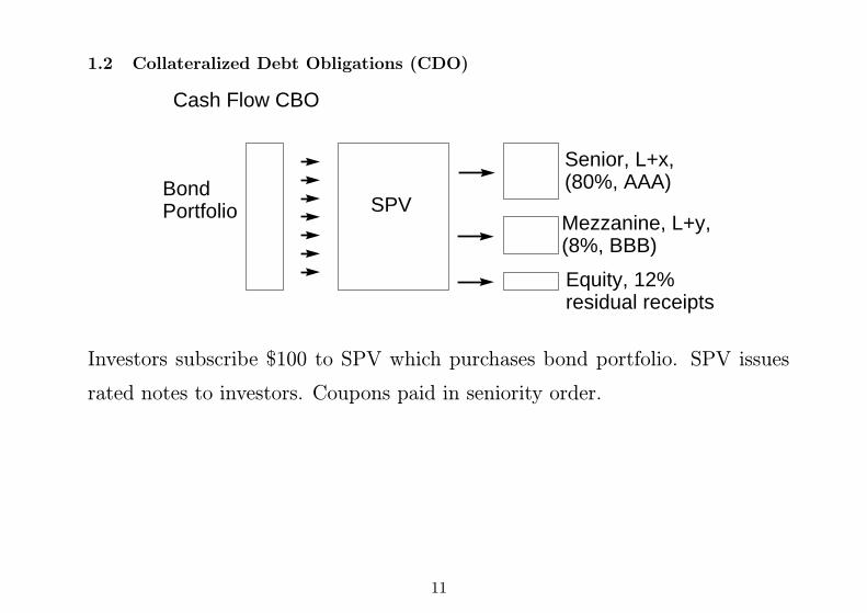
1.2 Collateralized Debt Obligations (CDO)

Cash Flow CBO

Senior, L+x,(80%, AAA)

Mezzanine, L+y,(8%, BBB)

Equity, 12%residual receipts

SPVBondPortfolio

Investors subscribe $100 to SPV which purchases bond portfolio. SPV issues

rated notes to investors. Coupons paid in seniority order.

11

Synthetic CDO

12-100%x

3-12%y

0-3%z

SPVCounter-party

Single-nameCDSs

Tranche CDSs

Here SPV sells credit protection to counterparty as individual-name CDS, buys

credit protection on tranches from investors with premiums x < y < z.

The joint default distribution is the key thing here.

New market product: iTraxx index – tranche quotes publicly available on

a standardised debt portfolio. Significance: market data directly related to

‘correlation’.

12

The design process for cash-flow CDOs

Cash Flow CBO

Senior, L+x,(80%, AAA)

Mezzanine, L+y,(8%, BBB)

Equity, 12%residual receipts

SPVBondPortfolio

• Set the size of the senior tranche as big as possible while satisfying expected

loss constraints needed to secure AAA credit rating (see below).

• Similarly for mezzanine tranches.

• Size of equity tranche is set by risk appetite of investors.

• Pricing (i.e. spreads) on rated tranches are determined by market condi-

tions on launch date.

13

1.3 The rating process: Moody’s Binomial Expansion Technique

Start with a portfolio ofM bonds, each (for simplicity) having the same notional

value X. Each issuer is classified into one of 32 industry classes. The portfolio

is deemed equivalent to a portfolio of M ′ ≤M independent bonds, each having

notional value XM/M ′. M ′ is the diversity score, computed from the following

table.

14

Diversity score table:

No. of firms Diversity Score

1 1.0

2 1.5

3 2.0

4 2.3

5 2.6

6 3.0

7 3.2

8 3.5

9 3.7

10 4.0

15

Diversity score example:

M = 60 bonds.

No. of firms in sector 1 2 3 4 5

No. of incidences 12 12 5 1 1

Diversity 12 18 10 2.3 2.6

Meaning: 12 cases where the firm is the only representative of its industry

sector, 12 pairs of firms in the same sector, etc.

Diversity score = 45.

The effect of reduced diversity is to push weight out into the tail of the loss

distribution, as the chart shows.

16

Binomial loss distributions

0

0.02

0.04

0.06

0.08

0.1

0.12

0.14

0.16

0.18

0 0.05 0.1 0.15 0.2 0.25 0.3 0.35 0.4 0.45 0.5Fraction of portfolio

d = 60d = 45d = 30

17

“Loss” in rated tranches

Suppose the coupon in a rated tranche is c and the amounts actually received

are a1, . . . , an. Then the loss is 1− q where

q =a1

1 + c+a2

1 + c+ ∙ ∙ ∙+

an

1 + c.

Note that q = 1 (loss zero) when ai = c, i < n and an = 1 + c.

Moody’s rates tranches on a threshold of expected loss.

Example: M = 60, p = 0.1.

Expected no. of defaults is μ = np = 6, standard deviation

σ =√np(1− p) = 2.32.

The senior tranche might have a loss threshold of μ+ 3σ = 13.

Chart shows expected loss as function of diversity score. Expected loss in-

creases by a factor of 10 as diversity score is reduced from 60 to 30.

18

Expected Loss in Senior Tranche

0

0.005

0.01

0.015

0.02

0.025

0.03

0.035

0.04

0.045

0.05

30 31 32 33 34 35 36 37 38 39 40 41 42 43 44 45 46 47 48 49 50 51 52 53 54 55 56 57 58 59 60

Diversity Score

19

1.4 CreditMetrics

CreditMetrics is aimed at producing the Value-at-Risk over a 1-year time hori-

zon for – say – a bond portfolio. Assumptions:

• There is a fixed credit spread for each credit rating

• Change in value is due only to change in credit rating

• Change in credit rating follows the Moody’s 1-year transition matrix.

What about correlation?

• There are N industry sectors and each obligor i has a weight N -vector wi

such that wi,j represents the participation of obligor i in sector j.

• CreditMetrics estimates the equity return correlation for sector indices

I1, . . . , IN , giving a correlation matrix Q.

20

• The return for obligor i is

ri = wi,0ri,0 +N∑

j=1

wi,jRj

where Rj is the normalized return for sector index Ij and ri,0 is an idiosyn-

cratic factor.

• The obligor correlations are

ρik = corr(ri, rk) =wTi Qwk√

(wTi Qwi + w2i,0)(w

TkQwi + w

2k,0)

• Generate a normal M -vector X with mean 0 and covariance matrix A with

diagonal elements 1 and off-diagonal elements ρik.

• Choose quantiles in each coordinates direction so that Xi gives the correct

transition probabilities for obligor i (see picture)

21

BBB

BBB

BBB A AA

A

AA

BBB

Obligor 1

Obligor 2

This procedure gives the joint transition probabilities for all obligors. (In

the figure, Obligor 1 starts at BBB, obligor 2 at A.)

22

2 Joint distributions, Hazard Rates and Copulas

Let τ ≥ 0 be a random variable with density f(t). The survivor function G

and distribution function F are

P [τ > t] = G(t) = 1− F (t) =∫ ∞

t

f(u)du.

The hazard rate is

h(t)dt =f(t)

G(t)dt ≈ P [τ ∈]t, t+ dt]|τ > t],

and there is a 1-1 relation between h and G in that

G(t) = e−∫ t0h(u)du.

Thus specifying h is equivalent to specifying f .

23

For random variables τ1, τ2 ≥ 0 with joint density f(t1, t2) the marginal and

joint distributions are

F1(t) =

∫ t

0

∫ ∞

0

f(u, v)dv du

F2(t) =

∫ ∞

0

∫ t

0

f(u, v)dv du

F (t1, t2) =

∫ t1

0

∫ t2

0

f(u, v)dv du,

while the survivor function is

G(t1, t2) =

∫ ∞

t1

∫ ∞

t2

f(u, v)dv du

The joint distribution F is related to the marginals by the copula function C

given by

F (t1, t2) = C(F1(t1), F2(t2)). (1)

Given marginal distributions F1, F2, formula (1) defines a bone fide joint distri-

bution for any choice of copula function C.

24

Let τmin = min(τ1, τ2), τmax = max(τ1, τ2). Then

P [τmin > t] = G(t, t).

The initial hazard rate is therefore (see picture)

h0(t) =1

G(t, t)

(∫ ∞

t

f(u, t)du +

∫ ∞

t

f(t, v)dv

)

t t+dt

t+dtt

25

Suppose τ1 occurs first. The conditional density of τ2 is then

f(τ1, t)∫∞τ1f(τ1, v)dv

for t ≥ τ1, so that the new hazard rate is

h2(t) =f(τ1, t)∫∞

tf(τ1, v)dv

,

while if τ2 occurs first the hazard rate switches to

h1(t) =f(t, τ2)∫∞

tf(u, τ2)du

.

The hazard rate process is therefore

h(t) = h0(t)1(t<τmin) +(h2(t)1(τmin=τ1) + h1(t)1(τmin=τ2)

)1(τmin≤t<τmax)

26

2.1 Copula-based calibration

Let τ1, τ2, . . . default times of issuers A, B, . . .. If F is the joint distribution

and Fi is the marginal distribution of τi then

F (t1, . . . , tn) = C(F1(t1), . . . , Fn(tn))

for some copula function C (= a multivariate DF with uniform marginals).

(i) Back out marginal default distributions F1(t), F2(t), . . . from credit spreads

or CDS rates.

(ii) Choose your favourite copula function – say, Gaussian copula.

(iii) Take correlation parameter ρ = correlation of equity returns.

(iv) Define joint distribution F as above.

27

In more detail:

(i) In a CDS contract, protection buyer pays regular premiums π until min(τ, T )

where T is the contract expiry time and τ the default time of the Reference

Bond. Protection seller pays (1 − R)1(τ<T ) at next coupon date after τ , where

R is the recovery rate. If F is the risk-neutral survivor function of τ , the ‘fair

premium’ π is determined by

n∑

i=1

πp(0, ti)F (ti) = π × CV01 =n∑

i=1

(F (ti−1)− F (ti))(1−R)p(0, ti).

If we have CDS rates πk for maturities Tk, k = 1, . . . ,m and a family of distri-

butions {Fθ, θ ∈ Rm} then we can determine the ‘implied default distribution’

Fθ̂.

28

A standard procedure is to take

Fθ(t) = exp

(

−∫ t

0

h(s)ds

)

where

h(s) =m∑

i=1

θi1]Ti−1,Ti](s).

Then θi, θ2, . . . are determined recursively using π1, π2, . . ..

Note: in a multivariate setting there is a different parametrization Fj,θj for

each issuer.

(ii),(iii) To generate a random vector U with uniform marginals and a gaussian

copula, take Ui = N−1(Xi) where X is a normal random vector with EXi =

0,EX2i = 1,EXiXj = ρij.

29

NB: Care must be taken that the covariance matrix

Σ =

1 ρ11 ρ12 . . .

ρ21 1 ρ23 . . .............

is actually non-negative definite. If the ρij are obtained from sample estimates,

it may not be!

To generate X, take X = AZ where A is the Cholesky factorization of Σ

(i.e. Σ = AAT) and Zi are independent N(0, 1). In the 2-dimensional case we

can simply take X1 = Z1, X2 = ρ12Z1 +√1− ρ212Z2.

(iv) Default times τi are given by

τi = F−1i,θi(Ui).

(There is an obvious algorithm for computing this when Fi,θ is as above.)

30

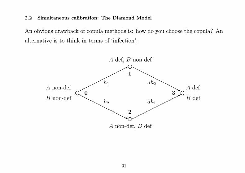
2.2 Simultaneous calibration: The Diamond Model

An obvious drawback of copula methods is: how do you choose the copula? An

alternative is to think in terms of ‘infection’.

0

1

2

3A non-def

B non-def

A def

B def

A def, B non-def

A non-def, B def

h1 ah2

h2 ah1

31

• Hazard rate of remaining issuer increases by a factor a after first default.

• If functions h1, h2 are time-dependent and we replace ah1, ah2 by general

h3, h4 then we can represent any joint distribution this way.

32

Marginal distributions

F1(t) = 1− e−(h1+h2)t −

h2e−ah1t

h1 + h2 − ah1

(1− e−(h1+h2−ah1)t

)

F2(t) = 1− e−(h1+h2)t −

h1e−ah2t

h1 + h2 − ah2

(1− e−(h1+h2−ah2)t

)

Double Default

FDD(t) = 1− e−(h1+h2)t −

h2e−ah1t

h1 + h2 − ah1

(1− e−(h1+h2−ah1)t

)

−h1e

−ah2t

h1 + h2 − ah2

(1− e−(h1+h2−ah2)t

)

Calibration

Joint calibration to credit spreads/CDS rates for issuers A and B, for given

‘enhancement’ parameter a. (Time-varying h1, h2 required for term structure

of credit spreads)

33

Continuous-time CDS premium πi on asset i is determined by

πi

∫ T

0

e−rt(1− Fi(t))dt = (1−R)∫ T

0

e−rtfi(t)dt,

where r is the riskless rate and fi(t) = dFi(t)/dt. From the model, we find

π1 = (1−R)I2

I1

where (with m(α, T ) = 1α(1− e−αT ))

I1 = h1(1− a)m(r + h1 + h2, T ) + h2m(r + ah1, T ),

I2 = (h1 + h2)h1(1− a)m(r + h1 + h2, T ) + ah1h2m(r + ah1, T ).

The first default time τmin = τ1 ∧ τ2 is exponential with rate (h1 + h2). Hence

the FTD premium is

πFTD = (1−R)(h1 + h2).

Chart shows calibrated h1, h2 when CDS rates are π1 = 75bp, π2 =200bp.

34

Calibrated parameters h1, h2, and First-to-Default premium

0

0.005

0.01

0.015

0.02

0.025

0.03

0.035

1 2 3 4 5 6 7 8enhancement factor a

h1h2FTD

35

Generators and Backward Equations

The generator of a Markov process xt is an operator A acting on functions

D(A) such that

M ft = f(xt)− f(x0)−∫ t

0

Af(xs)ds

is a martingale for f ∈ D(A). The corresponding backward equation is

∂v

∂t+Av − βv = 0

v(T, x) = h(x)

The solution of the backward equation is

v(t, x) = Et,x

[e−

∫ Ttβ(xs)dsh(xT )

]

(as in Black-Scholes).

36

For the diamond model, xt ∈ {0, 1, 2, 3} and the generator can be expressed in

matrix form as

A =

−(hA + hB) hA hB 0

0 −βhB 0 βhB

0 0 −αhA αhA

0 0 0 0

.

Solving the backward equation amounts to computing the matrix exponential

eAt. We can also solve the forward equation

d

dtp(t) = p(t)A

for the probability distribution of the process at time t (expressed as a row

vector)

Other, more complex, models are also easily computable.

37