Population Invariance of Test Equating and Linking: Theory Extension and Applications Across Exams

October 2006 RR-06-31

ResearchReport

Edited by

Alina A. von Davier

Mei Liu

Research & Development

Population Invariance of Test Equating and Linking:

Theory Extension and Applications Across Exams

Edited by

Alina A. von Davier and Mei Liu

ETS, Princeton, NJ

Papers by

Xiaohong Gao, Deborah Harris, and Nancy Petersen

ACT, Inc., Iowa City, IA

Alina A. von Davier, Neil J. Dorans, Rui Gao, Shelby Hammond, Paul W. Holland, Jinghua Liu,

Mei Liu, Christine Wilson, and Wen-Ling Yang

ETS, Princeton, NJ

Qing Yi

Harcourt Assessment, Inc., San Antonio, TX

Robert Brennan

University of Iowa, Iowa City, Iowa

October 2006

As part of its educational and social mission and in fulfilling the organization's nonprofit charter

and bylaws, ETS has and continues to learn from and also to lead research that furthers

educational and measurement research to advance quality and equity in education and assessment

for all users of the organization's products and services.

ETS Research Reports provide preliminary and limited dissemination of ETS research prior to

publication. To obtain a PDF or a print copy of a report, please visit:

http://www.ets.org/research/contact.html

Copyright © 2006 by Educational Testing Service. All rights reserved.

ETS and the ETS logo are registered trademarks of Educational Testing Service (ETS). ADVANCED

PLACEMENT PROGRAM, AP, COLLEGE BOARD, COLLEGE-LEVEL EXAMINATION PROGRAM, CLEP,

and SAT are registered trademarks of the College Board.

Abstract

One of the fundamental requirements of equating functions is that they should be population

invariant. Dorans and Holland (2000) introduced general measures for evaluating population

invariance by comparing linking functions obtained on subpopulations with those obtained on the

full population. Their discussion was restricted to data collection designs involving a single

population. This report contains a collection of related papers from five different testing programs

that use a variety of equating/linking settings, data collection designs, tests structures, and equating

methods to assess the degree of invariance of subpopulation equating results from total population

equating results. The measures of population invariance show promise as valuable tools for

evaluating the equatability of tests. Earlier versions of these papers were presented at a symposium

at the 2004 annual meeting of the National Council on Measurement in Education.

Key words: Anchor test design, score equating, IRT equating, groups differences, population

invariance, test linking, RMSD

i

Acknowledgments

The authors would like to thank Kim Fryer for her extensive editorial help.

ii

Table of Contents

Preface………………………………………………………………………………………….... v

Population Invariance of IRT True Score Equating by Alina A. von Davier and

Christine Wilson…………………………………………………………………………….….…1

Exploring the Population Sensitivity of Linking Functions Across Test Administrations

Using LSAT Subpopulations by Mei Liu and Paul W. Holland….…………………………......29

Invariance of Score Linkings Across Gender Groups for Forms of a Testlet-Based

CLEP® Examination by Wen-Ling Yang and Rui Gao…………………………………...….....59

Invariance of Equating Functions Across Different Subgroups of Examinees Taking

a Science Achievement Test by Qing Yi, Deborah J. Harris, and Xiaohong Gao…………...….99

The Role of the Anchor Test in Achieving Population Invariance Across Subpopulations

and Test Administrations by Neil J. Dorans, Jinghua Liu, and Shelby Hammond…………….131

A Discussion of Population Invariance of Equating by Nancy S. Petersen……………….…...161

A Discussion of Population Invariance by Robert L. Brennan……………………….………..171

References……………………………………………………………………………………...191

iii

Preface

Test equating methods are statistical methods used to produce scores that are comparable across

different test forms that have been carefully constructed based on the same content and statistical

specifications. The term test linking will be used to refer to the general process of connecting the

scores on two different tests.

One of the fundamental requirements of equating functions is that they should be

population invariant. Dorans and Holland (2000) introduced general measures for evaluating

population invariance by comparing linking functions obtained on subpopulations with those

obtained on the full population. Their discussion was restricted to data collection designs involving

a single population. von Davier, Holland, and Thayer (2004a) extended the Dorans and Holland

measures to the non-equivalent-groups anchor test design (NEAT) and examined its application to

nonlinear equating methods. These measures of population invariance show promise as valuable

tools for evaluating the equatability of tests.

A set of studies reported in Dorans (2004a, 2003) examined the application of population

invariance measures and specific issues associated with the linking of test forms of Advanced

Placement Program® (AP®) examinations. The results indicated a need for expanding population

invariance research to include other linking methods and other exams, as well as to explore the

sensitivity of the Dorans and Holland population invariance measures to additional subpopulations

and other test features such as test format, content, context, administration, and use.

This report builds on and extends existent research on population invariance to new tests

and issues. We lay the foundation for a deeper understanding of the use of population invariance

measures in a wide variety of practical contexts. The invariance of linear, equipercentile and IRT

equating methods are examined using data from five testing programs—AP, ACT, the College-

Level Examination Program® (CLEP®), LSAT, and the College Board’s SAT® (SAT).

The five papers in this report address a variety of issues. The SAT paper examines the role

of the anchor test in achieving population invariance of linear equatings across male and female

subpopulations and test administrations. The AP paper examines IRT models applied to exams

with both multiple-choice and constructed-response components. The CLEP paper investigates

population invariance of the 1-parameter IRT model applied to testlet-based computerized exams.

The LSAT paper extends the application of population invariance methods to subpopulations

defined by geographic region, whether examinees applied to law school, and their law school

v

admission status. Finally, the ACT paper examines the population invariance of a science test

across different ability groups using IRT true and observed score equating as well as equipercentile

equating methods.

These studies expand our knowledge about the Dorans and Holland invariance indices,

improve our understanding of population invariance, and provide practitioners with some

empirical benchmarks of the effects of different test features (such as test format, context,

administration, etc.); different equating designs; and different subpopulations on the invariance of

linking functions.

Nancy Petersen and Robert Brennan are two leading experts with extensive experience in

the theory and practice of test equating and linking. Petersen and Brennan’s publications are

valuable references for anyone who is learning or working in the area of test equating and linking.

See Kolen’s and Brennan’s book on testing equating, scaling, and linking (Kolen & Brennan,

2004) and the equating and scaling chapter that Nancy Petersen coauthored, which appeared in

Linn (1989). Petersen’s and Brennan’s comments conclude this volume.

Alina A. von Davier and Mei Liu

October 2006

vi

Population Invariance of IRT True Score Equating

Alina A. von Davier and Christine Wilson

ETS, Princeton, NJ

1

Abstract

Dorans and Holland (2000) and von Davier, Holland, and Thayer (2003) introduced measures of

the degree to which an observed score equating function is sensitive to the population on which it

is computed. This paper extends the findings of Dorans and Holland and of von Davier et al. to

item response theory (IRT) true score equating methods that are commonly used in the non-

equivalent-groups with anchor test (NEAT) design. Using data from the AP® Calculus AB exam,

which contain multiple choice (MC) and free responses (FR) sections, we investigate the

population sensitivity of the IRT equating functions computed for the MC section only and for

the MC and FR sections together. We also compare the degree of population sensitivity across

three equating methods: the IRT true score equating method and two observed score equating

methods, chained equipercentile and Tucker linear equating.

Key words: Population sensitivity, observed-score equating, IRT true-score equating, non-

equivalent-groups with anchor test (NEAT)

2

Acknowledgments

The authors thank Dan Eignor, Wendy Yen, Wen-Ling Yang, and Ming-Mei Wang for their

comments and suggestions on the previous versions of this paper. The authors thank Frederic

Robin for his help with additional computations.

3

Introduction and Objectives

Test equating methods are used to produce scores that are interchangeable across

different test forms. Item response theory (IRT; Cook & Petersen, 1987; Hambleton,

Swaminathan, & Rogers, 1991; Lord, 1980; Petersen, Cook, & Stocking, 1983; Petersen, Kolen,

& Hoover, 1989; and many others) has provided alternative ways to approach test equating. One

of the five requirements of equating functions mentioned in Dorans and Holland (2000) is that

equating should be population invariant. See Harris and Kolen (1986), Brennan and Kolen

(1987), Harris and Crouse (1993), and Petersen et al. (1989) for detailed discussions on equating

criteria. Dorans and Holland introduced a measure of the degree to which an observed score

equating function is sensitive to the population on which it is computed. This measure, the root

mean squared difference (RMSD), compares equating or linking functions computed on different

subpopulations with the function computed for the whole population. von Davier, Holland, and

Thayer (2003) generalized the RMSD measure to the non-equivalent-groups with anchor test

(NEAT) design.

This paper discusses and extends the findings of Dorans and Holland (2000); von Davier

et al. (2003), and; von Davier, Holland, and Thayer (2004b) to the item-response theory (IRT)

true score equating method (with the Stocking and Lord scaling approach, described in Stocking

& Lord, 1983) that is commonly used with the NEAT design.

The goals of this paper are

1. to adapt the RMSD formula to investigate the population sensitivity of IRT equating

functions;

2. to investigate the population sensitivity of the IRT equating functions for a multiple-

choice (MC) section only and for MC and free response (FR) sections together, both

of the AP Calculus AB exam with respect to two subgroups of interest, males and

females; and

3. to compare the RMSD results obtained for the IRT equating with the RMSD results

for alternative traditional equating methods, such as chained equipercentile and Tucker

linear equating, used with the AP test.

Real data from the AP® Calculus AB exam are used to illustrate the application of the

RMSD index to the IRT true score equating as well as the comparisons described above.

4

Method

In this section, we introduce our notations and briefly present the assumptions that

underlie the data collection design, the IRT model, and the equating methods. See von Davier

and Wilson (2005) for a detailed discussion of these assumptions. We also describe the particular

IRT models used in this study. In the next subsection we introduce the RMSD measures for

investigating the population sensitivity of the IRT equating function.

Notations, Assumptions, Models, and Methods

In the NEAT design, X and Y are the operational tests given to two samples from the two

populations P and Q, taking X and Y, respectively, and V is a set of common items, the anchor

test, given to both samples from P and Q. The anchor test score, V, can be either a part of both X

and Y (the internal anchor case) or a separate test (the external anchor case). The data structure

for the NEAT design is illustrated in Table 1 (see also von Davier et al., 2004a, 2004b).

Note that Table 1 describes the data collection procedure and does not refer to the tests

scores. The subscripts, P and Q, indicate the populations.

Table 1

Description of the Data Collection Design

X V Y

P a a X, V observed on P

Q a a Y, V observed on Q

The analysis of the NEAT design usually makes two assumptions (see also von Davier et

al., 2004a): There are two populations of examinees such that the examinees from P could take

Form X and the anchor V, and the examinees from Q could take Form Y and the anchor V. Two

samples are (assumed to be) independently and randomly drawn from P and Q, respectively.

The usual IRT models assume that the tests to be equated, X and Y, and the anchor, V, are

unidimensional and measure the same construct. For all items in these tests, the

unidimensionality, the local independence, and the monotonicity assumptions are made (see

Hambleton et al., 1991, for example). Under the assumptions above, IRT provides tools for

modeling the (conditional) probabilities of the correct responses to the items in a test for each

5

examinee that took that test. The three-parameter-logistic (3PL) model, which is fitted to the MC

items in this study, is described by

P (zni = 1 | θn, ai, bi, ci) = ci + (1 - ci) logit-1[ai (θn - bi )] (1)

where zni denotes the answer of the person n to the item i, logit-1(·) = exp(·) / [1 + exp(·)], and a’s,

b’s, and c’s are the item parameters; θ is the person parameter (ability or competency of interest);

and P (zni = 1 | θn, ai, bi, ci) is the conditional probability of a correct answer of the person n to

the item i (see Hambleton et al., 1991 or Lord, 1980 for details).

The generalized partial credit model (GPCM; Muraki, 1992) is the IRT model that it is

fitted to the data containing FR items in this study. The GPCM for the polytomous items (with m

+1 categories, for example) is based on the assumption that each probability of choosing the k-th

category over the (k-1)-th category follows a dichotomous model (with k between 1 and m + 1).

j

0m

=0 1

exp[ ( - )] ( 1 | , , ) =

exp[ ( - )]

k

i n i

nik n i ik

i n i

a bP z a b

a b

νν

λ

νλ ν

θθ

θ

=

=

=∑

∑ ∑ (2)

where bi0 = 0 (arbitrarily fixed to 0). The threshold parameters in the partial credit model, bik, are

the intersection points between the probability curves Pnik and Pnik-1 (see Muraki).

Table 1 shows that in the NEAT design X is not observed in population Q, and Y is not

observed in population P. To overcome this feature, all equating and linking methods developed

for the NEAT design (both observed score and IRT methods) must make additional assumptions

that do not arise in the other linking designs. The assumption that the IRT models make for the

NEAT design is this: If the model fits the data in each of the two populations, then the item

parameters of the common items are population invariant (up to a linear transformation).

If the calibration was carried out separately on the two samples from the two different

populations P and Q, then two sets of parameter estimates for the anchor test items are obtained.

The two separate sets of parameter estimates for the anchor items in the two groups need to be

placed on the same scale. There are various methods for obtaining this scale transformation—

mean-mean, mean-sigma methods, or characteristic curve methods such as the Haebara (1980)

and Stocking and Lord (1983) methods.

6

As mentioned above, in this study we use the 3PL model for MC items and the GPCM

for the FR items. The characteristic curve method (Stocking & Lord, 1983) is used to place the

separately estimated parameters onto a common scale. Then the true score equating method is

used to obtain equivalent scores on X and Y (see Petersen et al., 1989; Kolen & Brennan, 2004;

von Davier & Wilson, 2005).

The IRT equating requires that the tests are number right scored, which involves an

implicit assumption that there are no omits (see Kolen & Brennan, 2004). If the tests are formula

scored, then some sort of transformation is necessary; this transformation will treat the omits as

wrong. Moreover, IRT calibration assumes that if the IRT model fits the data from the two

populations, then the item parameters of the common items are population invariant (up to a

linear transformation).

The IRT true score equating introduces one more assumption: The relationship between

the true scores holds also for the observed scores. Hence, the study of the population sensitivity

of the IRT true score equating function relies on the set of assumptions mentioned above. See

von Davier and Wilson (2005) for details.

The observed score equating functions investigated in this study, chained equipercentile

and Tucker, also make assumptions in order to overcome the missing-by-design data, a feature of

the NEAT design. We will not give any computational details for the two observed score

equating methods, since they are well-known. We give the assumptions for the two methods in

order to emphasize that all equating methods for the NEAT design require some (nontestable)

assumptions to be fulfilled. The assumptions and the formulas for the chained equipercentile

equating and for the Tucker linear equating are given in von Davier (2003), von Davier et al.

(2004a, 2004b), and Kolen and Brennan (2004).

Chained equating assumes that the linking functions, from X to V and from V to Y, are

population invariant; the Tucker equating assumes that the linear regressions of X on V and of Y

on V are population invariant and that the conditional variances of X given V and of Y given V

are population invariant.

Measures of Population Invariance

In this subsection, we recall the formulas for the population invariance measures

introduced by Dorans and Holland (2000) for data collection designs that rely on one population

of examinees and the measures introduced by von Davier et al. (2003) for the NEAT design,

7

where the examinees are drawn from two populations. Then, we will adapt the RMSD formulas

to accommodate the NEAT design in conjunction with the IRT equating function.

Measures of population invariance of an observed score equating function when there is

only one population underlying the data collection design. Dorans and Holland (2000)

introduced a measure of the degree to which an equating function is sensitive to the population

on which it is computed. This measure, the root mean squared difference (RMSD), compares

equating or linking functions computed on different subpopulations with the function computed

for the whole population. The formula introduced by Dorans and Holland is applicable to the

equivalent-groups and single-group designs, where the sample(s) are drawn from one population,

P. The formula for the RMSD is given below.

2( ) ( )

RM SD ( ) ,

w e x e xP Pjj jx

YPσ

⎡ ⎤−∑ ⎢ ⎥

⎣= ⎦ (3)

where x in (3) denotes a score value of the test X, P is the target population in the equivalent-

groups and single-group designs, which is the population from which the sample(s) were drawn.

In (3), eP denotes the equating function that equates X to Y on the whole population P; ePj

denotes the equating function that equates X to Y on the subpopulation Pj of P. The denominator,

σYP, is the standard deviation of Y in P. The weight wj might denote the relative proportion of Pj

in P, but other weights might be used as well. von Davier et al. (2004b) present arguments for

giving equal weight, wj, to each subpopulation link for computing the RMSD values.

To obtain a single number summarizing the values of the RMSD(x), Dorans and Holland

(2000) also introduced the expected root mean square difference, by averaging over the

distribution of X in P before taking the square root:

2( ) ( )

REM SD .

w E e x e xP Pj Pj j

YPσ

⎧ ⎫⎡ ⎤⎪ ⎪−∑ ⎨⎢ ⎥ ⎬⎪⎣ ⎦ ⎪⎩= ⎭ (4)

In (4), x denotes a random X-score sampled from the base population, P, and EP { }

denotes averaging over this distribution.

Measures of population invariance of an observed score equating function when there

are two populations underlying the data collection design. von Davier et al. (2004b) generalized

8

RMSD for observed score equating for the NEAT design. As mentioned earlier, in the NEAT

design there are two populations from which the samples of examinees are drawn. T denotes the

target population in the NEAT design (see Braun & Holland, 1982, or Kolen & Brennan, 2004)

for a discussion of the concept of a target population) and is defined as

T = wP + (1 – w)Q , (5)

where w, which can have values between 0 and 1, is the weight given to P. There are

subpopulations, {Pj} and {Qj}, that partition the base populations, P and Q, respectively, into

mutually exclusive and exhaustive subpopulations (such as males and females, or race/ethnicity).

Pj and Qj refer to the same type of subpopulations (e.g., males) of P and Q. Each Pj (and Qj) has

a nonnegative weight, wPj (and wQj, respectively), which could be its relative proportion in P

(and Q), or some other set of weights that sum to unity. This is denoted by

P = j∑ wPjPj and Q =

j∑ wQjQj, (6)

Where the weights, wPj and wQj, are allowed to be different in P and Q, if necessary. The target

subpopulations, Tj, are defined, following (5), as

Tj = wPj + (1 – w)Qj , (7)

where the same common weight, w, as in (5) was used to define the target subpopulations,{Tj}.

The weights for the RMSD formula can be computed as

wj = w(wPj) + (1 – w)wQj, (8)

or they might be set equal (von Davier et al., 2004b).

Let eTj(x) be a function that equates X to Y on Tj and eT(x) be a function that equates X to

Y on T. Both equating functions eTj(x) and eT(x) are assumed to be computed in the same way

(i.e., both are chained equipercentile functions or both are Tucker functions). RMSD(x) is

defined by von Davier et al. (2004b) as

2( ) ( )

RM SD ( ) ,

w e x e xT Tjj jx

YTσ

⎡ ⎤−∑ ⎢ ⎥

⎣= ⎦ (9)

where the choice of the denominator, σYT, depends on the equating method and on the

assumptions the method makes. Since Y is not observed in T, the standard deviation of Y in a

9

target population, T, is computed following the assumptions of the equating method. For

example, the σYT can be computed following the Tucker method (see Kolen & Brennan, 2004) or

the σYT can be computed following the chained linear equating method (since σYT is a parameter

in the chained linear equating function, see von Davier et al., 2004b).

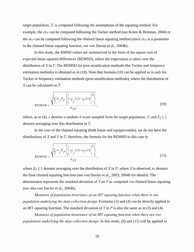
In this study, the RMSD values are summarized in the form of the square root of

expected mean squared differences (REMSD), where the expectation is taken over the

distribution of X in T. The REMSD for post-stratification methods (the Tucker and frequency

estimation methods) is obtained as in (10). Note that formula (10) can be applied as is only for

Tucker or frequency estimation methods (post-stratification methods), where the distribution of

X can be calculated on T.

2( ) ( )

REM SD ,

w E e x e xT Tj Tj j

YTσ

⎧ ⎫⎡ ⎤⎪ ⎪−∑ ⎨⎢ ⎥ ⎬⎪⎣ ⎦ ⎪⎩= ⎭ (10)

where, as in (4), x denotes a random X-score sampled from the target population, T, and ET { }

denotes averaging over this distribution in T.

In the case of the chained equating (both linear and equipercentile), we do not have the

distributions of X and Y in T; therefore, the formula for the REMSD in this case is

2( ) ( )

REM SD ,

w E e x e xT Tj Pj j

YTσ

⎧ ⎫⎡ ⎤⎪ ⎪−∑ ⎨⎢ ⎥ ⎬⎪⎣ ⎦ ⎪⎩= ⎭ (11)

where EP { } denotes averaging over the distribution of X in P, where X is observed. eT denotes

the final chained equating function (see von Davier et al., 2003; 2004b for details). The

denominator represents the standard deviation of Y on T as computed via chained linear equating

(see also von Davier et al., 2004b).

Measures of population invariance of an IRT equating function when there is one

population underlying the data collection design. Formulas (3) and (4) can be directly applied to

an IRT equating function. The standard deviation of Y in P is also the same as in (3) and (4).

Measures of population invariance of an IRT equating function when there are two

populations underlying the data collection design. In this study, (9) and (11) will be applied to

10

the IRT based equating method. More precisely, the weights are defined as in (8), and the

subpopulations are defined as in (6).

The IRT based equating function, eIRT(x), will be computed for all examinees, as well as

for each subpopulation of interest Tj, eIRT;j(x). Given the IRT model and the IRT true score

equating assumptions mentioned in the previous subsection and the way the IRT true score

equating is computed, it is not obvious which is the target population. This aspect is reflected in

the formulas we use for the RMSD and REMSD. For example, the denominator will be σYQ,

because this is the only place where we can compute the standard deviation for Y under the

assumptions described above. If the differences between the distributions of X and Y in the two

populations, P and Q, are large, we might alternately consider σ(eIRT;j(x)), which is the standard

deviation of the equated X.

For comparison purposes, one might use different denominators, where the standard

deviation of Y in a synthetic population T is computed following the assumptions of other

equating methods: the σYT computed as given by the Tucker method (see Kolen & Brennan,

2004) or σYT as given by the chained linear equating method (see von Davier et al., 2004b).

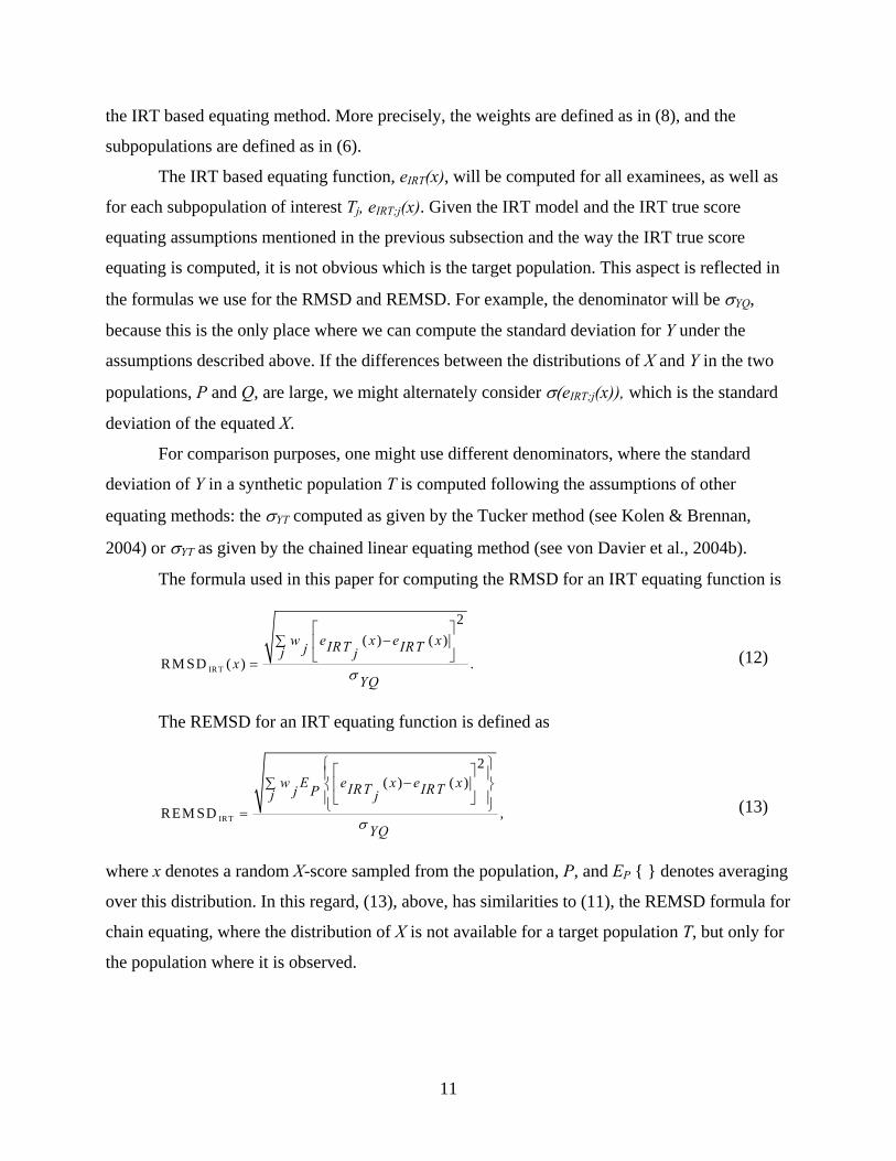
The formula used in this paper for computing the RMSD for an IRT equating function is

IRT

2( ) ( )

RM SD ( ) .

w e x e xIRT IRTjj jx

YQσ

⎡ ⎤−∑ ⎢ ⎥

⎣= ⎦ (12)

The REMSD for an IRT equating function is defined as

IRT

2( ) ( )

REM SD ,

w E e x e xIRT IRTj Pj j

YQσ

⎧ ⎫⎡ ⎤⎪ ⎪−∑ ⎨⎢ ⎥ ⎬⎪ ⎣ ⎦ ⎪⎩= ⎭ (13)

where x denotes a random X-score sampled from the population, P, and EP { } denotes averaging

over this distribution. In this regard, (13), above, has similarities to (11), the REMSD formula for

chain equating, where the distribution of X is not available for a target population T, but only for

the population where it is observed.

11

Data

In this section we describe the data used for investigation of the population sensitivity of

IRT equating functions.

The data are from the 2003 and 2001 administrations of the AP Calculus AB exam. In

these data sets there were 163,142 examinees in the 2003 administration and 145,415 examinees

in the 2001 administration. These data contain all the examinees that took the regular forms of

the AP Calculus AB exam in 2003 and 2001, respectively; the operational data contain

subsamples from each of these larger samples.

This AP exam uses a NEAT design with the 2003 test being equated back to 2001. The

anchor test, V, is an internal anchor within the MC component of the whole test. The whole MC

sections (the whole tests, X and Y) have 45 items each; the (internal) anchor has 15 items.

Each particular AP Calculus AB exam has a composite score, which is a weighted sum of

scores from MC and FR parts. For the AP Calculus AB exam, the FR section contains six items,

each with 10 possible score categories (from 0 to 9).

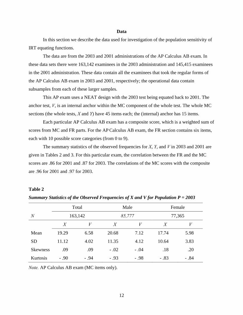
The summary statistics of the observed frequencies for X, Y, and V in 2003 and 2001 are

given in Tables 2 and 3. For this particular exam, the correlation between the FR and the MC

scores are .86 for 2001 and .87 for 2003. The correlations of the MC scores with the composite

are .96 for 2001 and .97 for 2003.

Table 2

Summary Statistics of the Observed Frequencies of X and V for Population P = 2003

Total Male Female

N 163,142 85,777 77,365

X V X V X V

Mean 19.29 6.58 20.68 7.12 17.74 5.98

SD 11.12 4.02 11.35 4.12 10.64 3.83

Skewness .09 .09 - .02 - .04 .18 .20

Kurtosis - .90 - .94 - .93 - .98 - .83 - .84

Note. AP Calculus AB exam (MC items only).

12

Table 3

Summary Statistics of the Observed Frequencies of Y and V for Population Q = 2001

Total Male Female

N 145,415 76,606 68,809

Y V Y V Y V

Mean 18.56 6.30 19.69 6.83 17.31 5.71

SD 10.66 3.93 10.84 4.05 10.31 3.71

Skewness .10 .16 .02 .04 .16 .26

Kurtosis - .85 - .87 - .87 - .94 - .82 - .75

Note. AP Calculus AB exam (MC items only).

Operationally, the tests are scored using rounded formula scoring. But for the purpose of

this study, the tests are scored number right, treating omits as wrong (see p. 7 for assumptions

required by IRT equtating). In this study, we focus only on the raw-to-raw score equating and not

on the raw-to-scale conversion.

The two subpopulations we examined were males (M) and females (F). In 2003 there

were 85,777 male and 77,365 female test takers, and in 2001 there were 76,606 male and 68,809

female test takers.

The effect size computations given in Table 4 show that the M/F differences are very

large, much larger than the differences between the two administrations.

Table 4

Effect Sizes for Male/Female Differences on the Anchor Test

Year Mean males

SD males

Mean females

SD females

Mean all

SD all

M-F means

Effect size

2003 7.12 4.12 5.98 3.83 6.58 4.02 1.14 28.7%

2001 6.83 4.05 5.71 3.71 6.30 3.93 1.12 28.9%

Note. Anchor-test data from the 2003 and 2001 administrations of the AP Calculus AB exam.

(MC items only).

13

The effect size for the difference between 2003 and 2001 for all examinees is (6.58–

6.30)/3.975 = 0.070 or 7% (3.975 is the average of 4.02 and 3.93). Thus, the 7% effect size for

the differences between the two years is much less than the M/F effect sizes for the differences in

each year.

The effect size for the difference between 2003 and 2001 for all male examinees (as

measured by the anchor) is (7.12-6.83)/[(4.12+4.05)/2]=0.071, or 7.1%, and the effect size for

the difference between 2003 and 2001 for all female examinees is also about 7%. The differences

reflected in the summary statistics for the common items suggest that the examinees from 2003

were more able than those from 2001.

The correlation between the test X (MC items only) and (internal) anchor test V in P

(2003) is 0.9087 and between Y (MC items only) and V in Q (2001) is 0.9278.

Tables 5 and 6 suggest (also taking into account the information from Tables 2 and 3)

that the FR section was more difficult in 2003 than in 2001 (for the total as well as for the

subpopulations).

Why AP Calculus AB Exam?

We selected Calculus AB for a few reasons: (a) This is an assessment where the IRT

assumptions seem to hold well enough (see the detailed analysis carried out in von Davier &

Wilson, 2005); (b) the differences in abilities between males and females as measured by the

anchor are very large (see Table 3), which might lead to a lack of population invariance of all

equating functions; and (c) Dorans, Holland, Thayer, and Tateneni (2003, pp. 89-97) investigated

the population sensitivity of the observed score equating functions that are operationally used for

the Calculus AB exam with respect to the gender subgroups. They found that the choice of

gender subpopulation did not affect the equating function or the grade assignment for the 1999 to

2000 forms of AP Calculus AB that were linked. However, for the link from 1998 to 1999, the

conversion functions for each subpopulation seemed to differ from the conversion for the total

group, and the grade assignment was affected as well. Hence, this study adds to the information

available for the equating process for the AP Calculus AB exam, and it might contribute to a

future analysis of the stability of equating functions over time.

14

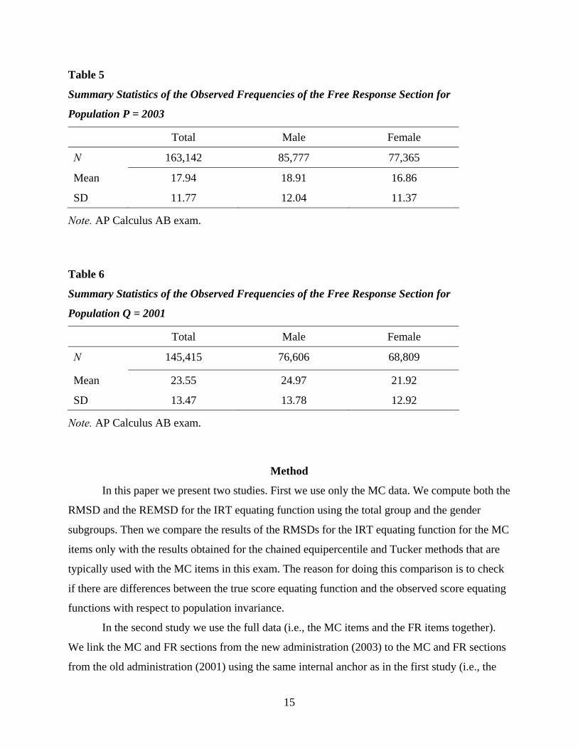
Table 5

Summary Statistics of the Observed Frequencies of the Free Response Section for

Population P = 2003

Total Male Female

N 163,142 85,777 77,365

Mean 17.94 18.91 16.86

SD 11.77 12.04 11.37

Note. AP Calculus AB exam.

Table 6

Summary Statistics of the Observed Frequencies of the Free Response Section for

Population Q = 2001

Total Male Female

N 145,415 76,606 68,809

Mean 23.55 24.97 21.92

SD 13.47 13.78 12.92

Note. AP Calculus AB exam.

Method

In this paper we present two studies. First we use only the MC data. We compute both the

RMSD and the REMSD for the IRT equating function using the total group and the gender

subgroups. Then we compare the results of the RMSDs for the IRT equating function for the MC

items only with the results obtained for the chained equipercentile and Tucker methods that are

typically used with the MC items in this exam. The reason for doing this comparison is to check

if there are differences between the true score equating function and the observed score equating

functions with respect to population invariance.

In the second study we use the full data (i.e., the MC items and the FR items together).

We link the MC and FR sections from the new administration (2003) to the MC and FR sections

from the old administration (2001) using the same internal anchor as in the first study (i.e., the

15

anchor consists of MC items only). As before, the calibration was done separately for the 2003

and 2001 populations, and the item parameters were placed on the same scale using the Stocking

and Lord approach. We do not make use of the composite score in this study. Extending an

existing IRT model to accommodate weights for the items might be a future research topic. The

goal of the second study is to investigate the effect of the FR section on the sensitivity of the

equating function with respect to subpopulations.

IRT equating is not employed operationally for the AP Calculus AB exam, so before

conducting an IRT based equating process, we checked if the assumption necessary for applying

an IRT model holds (see Cook & Eignor, 1991; Cook & Petersen, 1987; Jodoin & Davey, 2003;

and Petersen et al., 1983, 1989, for a detailed discussion of the robustness of the IRT equating

function). Although the unidimensionality and local independence assumptions might not strictly

hold with the data, the IRT models should be robust enough to be used in practical situations

(Cook, Dorans, Eignor, & Petersen, 1985; Cook & Petersen; and Thissen, Wainer, & Wang,

1994). We investigated the two tests as well as of the individual anchors from different

perspectives (see Hattie, 1985), including the dimensionality. The findings (see von Davier &

Wilson, 2005) indicated that the FR items seem to measure the same construct as the MC items

and we concluded that the assumption for the IRT models holds well enough for our analyses.

The item parameters from the two calibrations of the common item set (2003 and 2001) were

investigated. We plotted the item parameters to look for outliers (those items with estimates that

do not appear to lie on a straight line). Figures 1 and 2 show the item parameters, the slope, a-,

and the difficulty, b-parameters, for the first study (MC items only), for the calibration for the

total population, for the males, and for the females. It appears that there are no outliers. In

addition, there were no significant changes among the item parameters for the MC common

items in Study I versus Study II (including the FR section), nor in the items’ characteristic

curves.

The detailed analyses of the fit of the IRT models and of how well the assumptions

described above are met for this particular data set are given in von Davier and Wilson (2005).

16

AP Calculus AB

0.55

0.65

0.75

0.85

0.95

1.05

1.15

1.25

0.5 0.55 0.6 0.65 0.7 0.75 0.8 0.85 0.9 0.95 1 1.05 1.1 1.15 1.2 1.25

2001 A Parm

2003

A P

arm

Total

Males

Females

Figure 1. The slope parameters for the anchor items for the two administrations. Study I.

AP Calculus AB

-1.5

-1

-0.5

0

0.5

1

1.5

2

-1.25 -1 -0.75 -0.5 -0.25 0 0.25 0.5 0.75 1 1.25 1.5 1.75 2

2001 B Parm

2003

B P

arm

Tot al

Males

Females

Figure 2. The b-parameters for the anchor items for the two administrations. Study I.

17

Description of Population Invariance Analysis

In the first study, we focused only on the MC items. We computed the IRT true-score

equating function for all examinees. We repeated the calibration and the IRT true-score equating

process for the two subpopulations of interest, males and females. Then we computed the RMSD

values using the formula given in (12) with the standard deviation of Y in Q, σYQ, as the

denominator, and we plotted them. We also computed the REMSD value. The RMSD for the

Tucker linear and chain equipercentile functions were also computed, as explained before. We

chose equal weights (wj = 0.5) for males and females for computing the RMSD and the REMSD

values for all equating functions. See more details about choosing the weights in von Davier et

al. (2004b). Then we compared the REMSD value obtained for the IRT true-score equating on

the MC items with the REMSD values obtained for the observed score equating functions. Note

that the equating results for the Tucker and the chain equipercentile function are not the

operational equating results. The REMSD values are also compared with the standard difference

that matters (SDTM) that is described below.

In the second study, we computed the IRT true-score equating function for the whole

tests. Then, we repeated the computations for the males and the females. We computed the

RMSD as in (12), using the denominator as the standard deviation of the MC and FR sections in

Q. We also computed the REMSD value. As in the first study, the REMSD values are also

compared with the SDTM that is described below.

Dorans et al. (2003) used the notion of a difference that matters (DTM) in the score

reporting for the Calculus AB exam. The DTM for a particular exam depends on the reporting

scale. In AP there are two metrics of interest, the composite score metric and the AP grade scale.

The scale that we will be using in this study for reference is the composite score metric (although

we use the same weight for the MC items as for the FR items in this study). The unit of this score

scale is one point. Hence, a difference between equating functions larger than a half point on this

scale means a change in the reporting score, which could result in two different AP grades.

Therefore, a half point on this scale defines the DTM for this particular exam and for our studies.

All the results will be compared to the DTM of a half point. This means that the differences in

the equating function are compared to the DTM, and the RMSD needs to be compared with a

SDTM, which is the DTM divided by the same quantity as the denominator in the RMSD.

18

For Study I, where we use only the 45 MC items, and where the standard deviation of Y in

Q is 10.66, the SDTM is obtained by dividing 0.5 (the half score point) by 10.66, which is 0.047.

For Study II, where we use the 45 MC items and the 6 FR items (equally weighted), and

where the standard deviation of the new Y (MC+FR) in Q is 23.22, the SDTM is obtained by

dividing 0.5 (the half score point) by 23.22, which is 0.022.

Results

Study I

Figure 3 plots the three IRT conversion lines, one for the total group and two for the

subgroups; they fall very close to each other, and are almost linear. Figure 4 plots the differences

in the males-only equating and females-only equating from the equating computed for the whole

population.

IRT Conversions. Study I

0

10

20

30

40

0 5 10 15 20 25 30 35 40 45

X-Score

Equa

ted

Raw

Sco

re o

n R

efer

ence

TotalMalesFemales

Figure 3. The three IRT conversions (for the total population, males, and females). Study I.

19

Differences Plots. Study I

-0.5

0

0.5

1

0 5 10 15 20 25 30 35 40 45

X-score

Diff

eren

ce fr

om A

ll

M-All

F-All

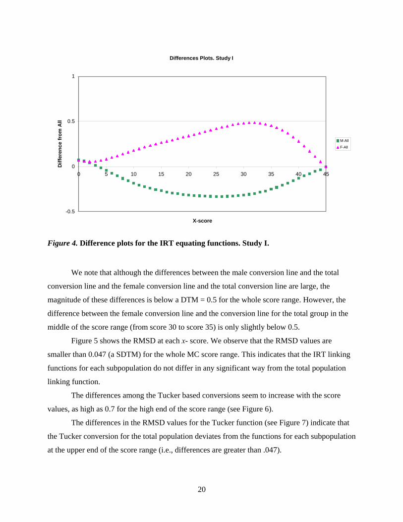
Figure 4. Difference plots for the IRT equating functions. Study I.

We note that although the differences between the male conversion line and the total

conversion line and the female conversion line and the total conversion line are large, the

magnitude of these differences is below a DTM = 0.5 for the whole score range. However, the

difference between the female conversion line and the conversion line for the total group in the

middle of the score range (from score 30 to score 35) is only slightly below 0.5.

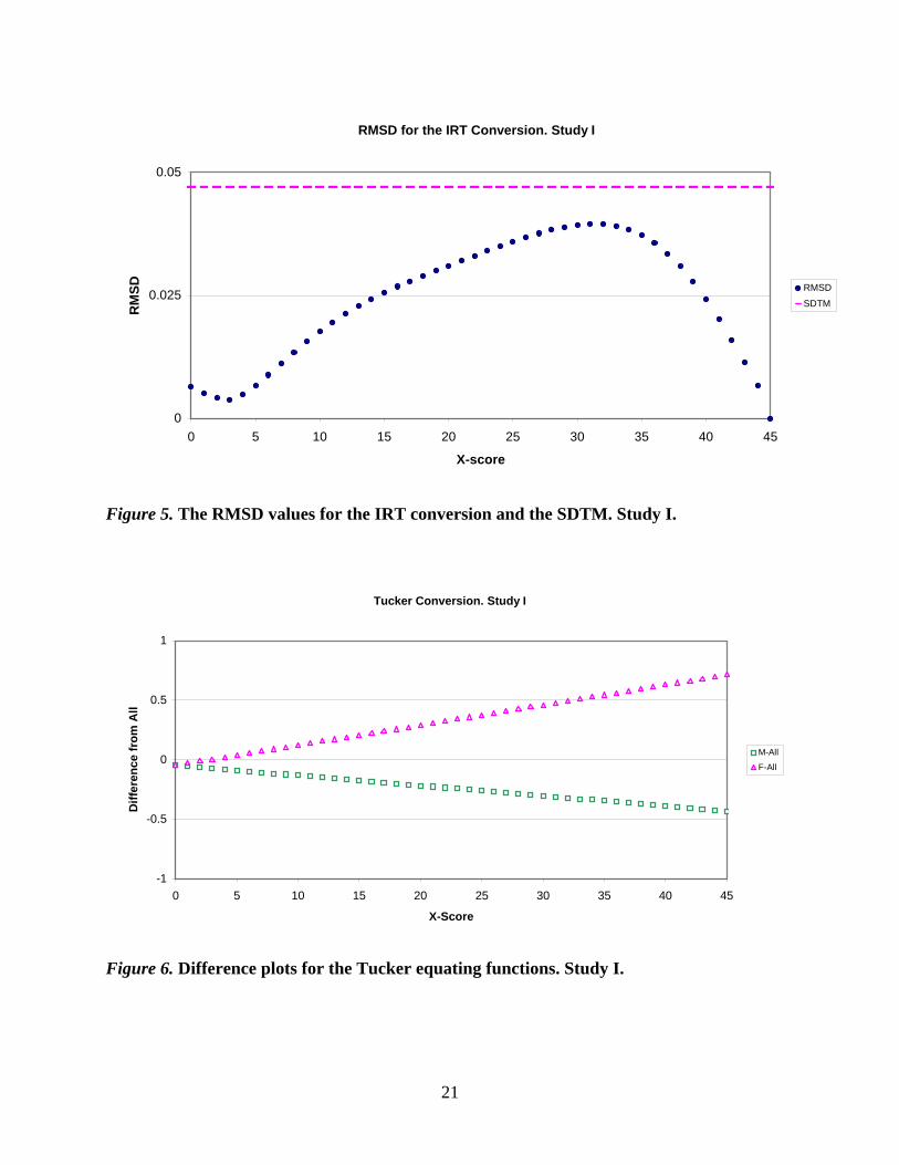
Figure 5 shows the RMSD at each x- score. We observe that the RMSD values are

smaller than 0.047 (a SDTM) for the whole MC score range. This indicates that the IRT linking

functions for each subpopulation do not differ in any significant way from the total population

linking function.

The differences among the Tucker based conversions seem to increase with the score

values, as high as 0.7 for the high end of the score range (see Figure 6).

The differences in the RMSD values for the Tucker function (see Figure 7) indicate that

the Tucker conversion for the total population deviates from the functions for each subpopulation

at the upper end of the score range (i.e., differences are greater than .047).

20

RMSD for the IRT Conversion. Study I

0

0.025

0.05

0 5 10 15 20 25 30 35 40 45

X-score

RM

SD RMSD

SDTM

Figure 5. The RMSD values for the IRT conversion and the SDTM. Study I.

Tucker Conversion. Study I

-1

-0.5

0

0.5

1

0 5 10 15 20 25 30 35 40 45

X-Score

Diff

eren

ce fr

om A

ll

M-All

F-All

Figure 6. Difference plots for the Tucker equating functions. Study I.

21

RMSD for the Tucker Function. Study I

0

0.02

0.04

0.06

0 5 10 15 20 25 30 35 40 45

X-Score

RM

SD RMSD

SDTM

Figure 7. RMSD values for the Tucker function and the SDTM. Study I.

The differences in the equating conversions for chained equipercentile (see Figure 8) and

the RMSD values for chained equipercentile conversions (Figure 9) indicate that the chained

equipercentile conversion and the IRT based conversion are population insensitive in a similar

manner: The differences among the conversions are larger in the middle of the score range, and

they are, in general, smaller than a SDTM of 0.047 for the whole score range.

Hence, from Figures 5, 7, and 9 that show the RMSD values at each x-score, we can

conclude that only the Tucker equating function presents some population sensitivity, and then

only at the upper part of the score range.

However, the three REMSD values for Study I are REMSD (IRT) = 0.0275, REMSD

(Tucker) = 0.0273, and REMSD (chained) = 0.0256. Each of the three REMSD values is smaller

than a SDTM, which suggests that on average each of the three methods is suitable for equating

these specific tests. It is surprising to see that the overall index, the REMSD, is lower for the

Tucker conversion than for the IRT conversion, although as the RMSD values indicate, the

Tucker conversion is the only conversion in Study I that presents some population dependency at

the upper range of raw scores. The discrepancy between the information reflected by the RMSD

and the REMSD is explained by the low frequencies at the high-end scores, because the REMSD

is an average result.

22

Chained Equipercentile Conversion. Study I

-1

-0.5

0

0.5

1

0 5 10 15 20 25 30 35 40 45

X-Score

Diff

eren

ce fr

om A

ll

M-All

F-All

Figure 8. Difference plots for the chained equipercentile equating functions. Study I.

RMSD for Chained Equipercentile Conversion. Study I

0

0.02

0.04

0.06

0 5 10 15 20 25 30 35 40 45

X-Score

RM

SD RMSD

SDTM

Figure 9. RMSD values for the chained equipercentile function and the SDTM. Study I.

23

Figure 10 shows the differences between the equating results for the Tucker, IRT, and the

chained equipercentile methods; the Tucker equating function was chosen as the criterion

equating in this plot. We see that there are two score points (42 and 43 for the difference between

Tucker and chained methods and 44 and 45 for the difference between Tucker and IRT methods)

where the differences exceed a DTM of 0.5. We also note that the differences between the

Tucker and the chained functions seem to be smaller than those between the Tucker and the IRT

functions for most of the score points.

Equating Differences. Study I

-1

-0.5

0

0.5

1

0 5 10 15 20 25 30 35 40 45

X-score

Diff

eren

ces

Tucker-IRT

Tucker-Chain

Figure 10. Equating differences between Tucker, IRT, and chained equipercentile

functions. Study I.

Study II

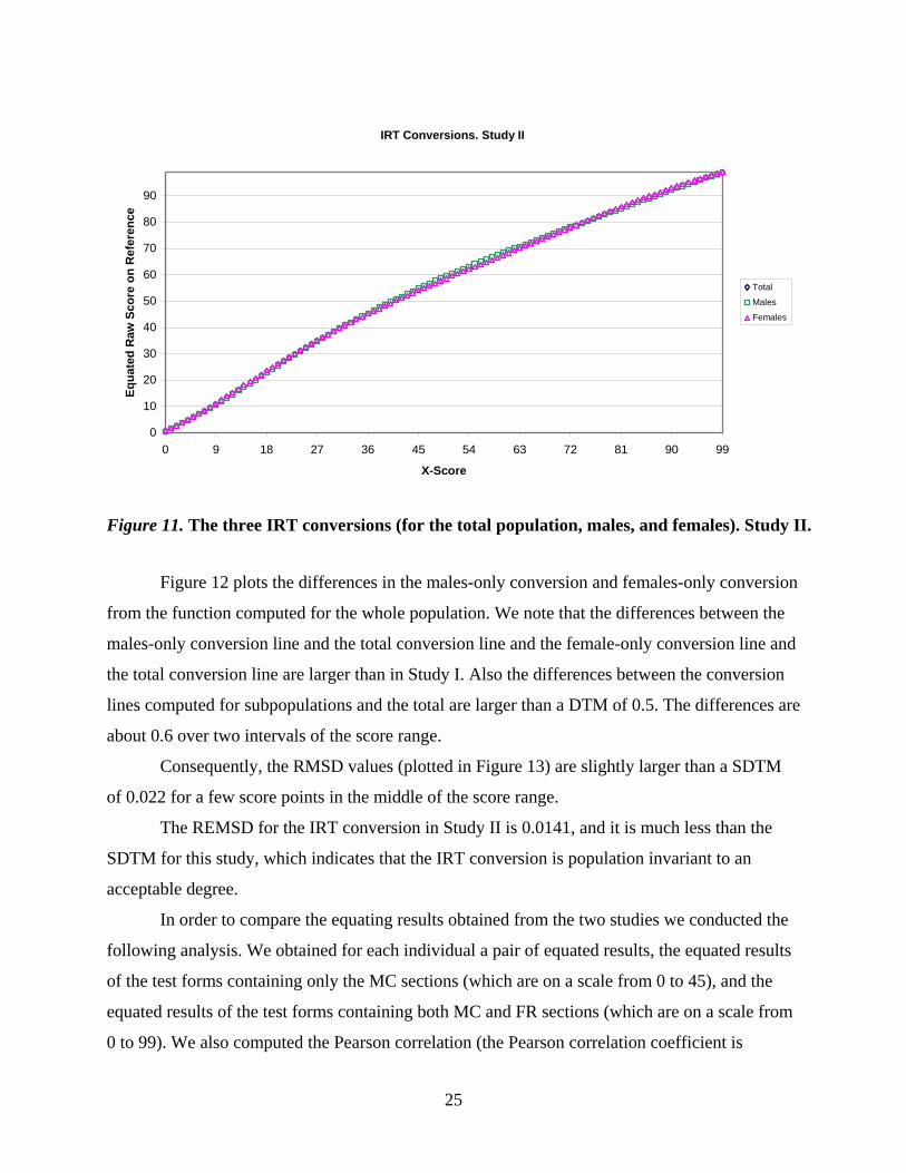
Figure 11 plots the three IRT conversion lines, one for the total population and two for

the subpopulations; they seem to be very close to each other, but, in contrast to the similar plot

for Study I (Figure 3), these three IRT conversions are obviously nonlinear, reflecting the

differences in the distributions of the two tests (mainly due to the differences in the FR sections).

24

IRT Conversions. Study II

0

10

20

30

40

50

60

70

80

90

0 9 18 27 36 45 54 63 72 81 90 99

X-Score

Equa

ted

Raw

Sco

re o

n R

efer

ence

Total

Males

Females

Figure 11. The three IRT conversions (for the total population, males, and females). Study II.

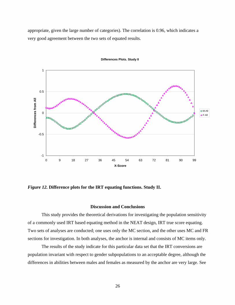
Figure 12 plots the differences in the males-only conversion and females-only conversion

from the function computed for the whole population. We note that the differences between the

males-only conversion line and the total conversion line and the female-only conversion line and

the total conversion line are larger than in Study I. Also the differences between the conversion

lines computed for subpopulations and the total are larger than a DTM of 0.5. The differences are

about 0.6 over two intervals of the score range.

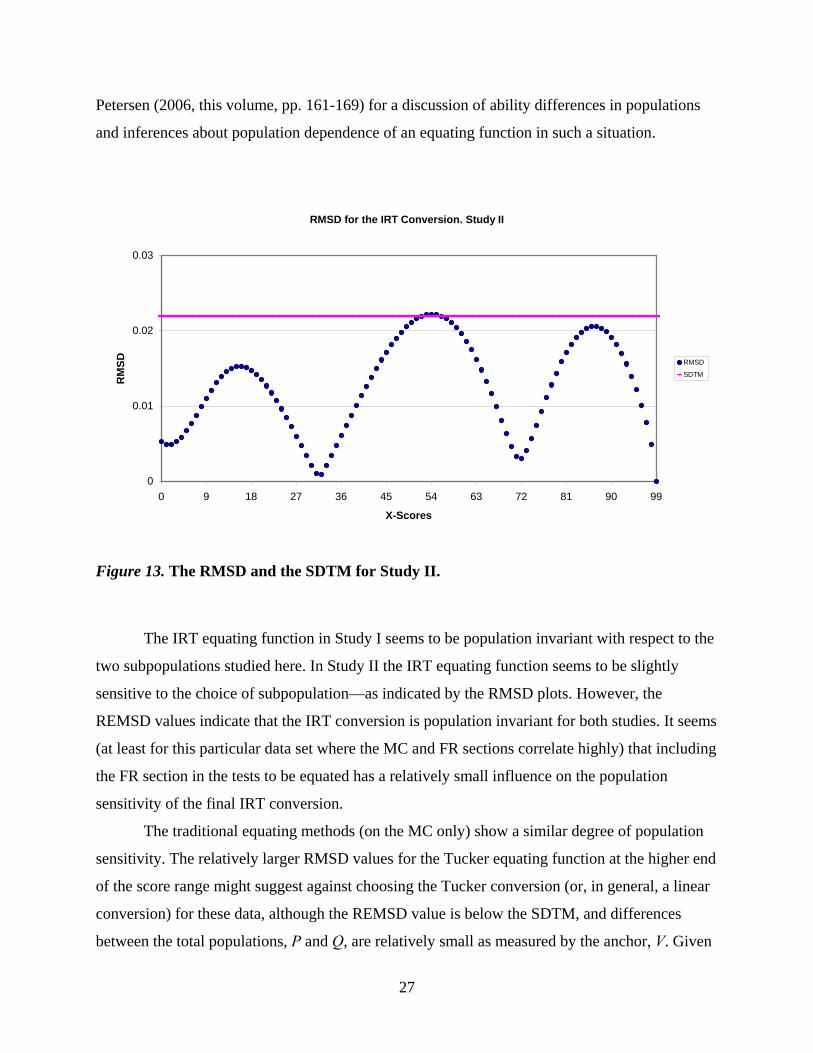
Consequently, the RMSD values (plotted in Figure 13) are slightly larger than a SDTM

of 0.022 for a few score points in the middle of the score range.

The REMSD for the IRT conversion in Study II is 0.0141, and it is much less than the

SDTM for this study, which indicates that the IRT conversion is population invariant to an

acceptable degree.

In order to compare the equating results obtained from the two studies we conducted the

following analysis. We obtained for each individual a pair of equated results, the equated results

of the test forms containing only the MC sections (which are on a scale from 0 to 45), and the

equated results of the test forms containing both MC and FR sections (which are on a scale from

0 to 99). We also computed the Pearson correlation (the Pearson correlation coefficient is

25

appropriate, given the large number of categories). The correlation is 0.96, which indicates a

very good agreement between the two sets of equated results.

Differences Plots. Study II

-1

-0.5

0

0.5

1

0 9 18 27 36 45 54 63 72 81 90 99

X-Score

Diff

eren

ces

from

All

M-All

F-All

Figure 12. Difference plots for the IRT equating functions. Study II.

Discussion and Conclusions

This study provides the theoretical derivations for investigating the population sensitivity

of a commonly used IRT based equating method in the NEAT design, IRT true score equating.

Two sets of analyses are conducted; one uses only the MC section, and the other uses MC and FR

sections for investigation. In both analyses, the anchor is internal and consists of MC items only.

The results of the study indicate for this particular data set that the IRT conversions are

population invariant with respect to gender subpopulations to an acceptable degree, although the

differences in abilities between males and females as measured by the anchor are very large. See

26

Petersen (2006, this volume, pp. 161-169) for a discussion of ability differences in populations

and inferences about population dependence of an equating function in such a situation.

RMSD for the IRT Conversion. Study II

0

0.01

0.02

0.03

0 9 18 27 36 45 54 63 72 81 90 99

X-Scores

RM

SD RMSD

SDTM

Figure 13. The RMSD and the SDTM for Study II.

The IRT equating function in Study I seems to be population invariant with respect to the

two subpopulations studied here. In Study II the IRT equating function seems to be slightly

sensitive to the choice of subpopulation—as indicated by the RMSD plots. However, the

REMSD values indicate that the IRT conversion is population invariant for both studies. It seems

(at least for this particular data set where the MC and FR sections correlate highly) that including

the FR section in the tests to be equated has a relatively small influence on the population

sensitivity of the final IRT conversion.

The traditional equating methods (on the MC only) show a similar degree of population

sensitivity. The relatively larger RMSD values for the Tucker equating function at the higher end

of the score range might suggest against choosing the Tucker conversion (or, in general, a linear

conversion) for these data, although the REMSD value is below the SDTM, and differences

between the total populations, P and Q, are relatively small as measured by the anchor, V. Given

27

the large sample sizes, we do not think that this observed population sensitivity is due to

sampling variability. In this situation, there is some imbalance in the data, as reflected in the fact

that the differences between the males and females vary across administrations. These

differences in the distributions might explain why a linear equating function might not capture

the relationship between the two tests in these particular populations, P and Q. However, given

that the REMSD value is very small and that the number of examinees at the higher scores is

low, the Tucker function might be considered for operational use as well.

Dorans et al. (2003) reported that the chained equipercentile equating for Calculus AB,

for the link between 1999 and 1998, is population sensitive with respect to gender

subpopulations and report no significant RMSD values for the link from 2000 to 1999. This is

similar to our results for both IRT and chained equipercentile conversions for the link between

2003 and 2001. These differences are difficult to explain without some measures of the standard

errors of the RMSD and REMSD statistics. While it is not appropriate to generalize too broadly

from this small number of studies, it does appear that the population sensitivity of an equating

function can vary over administrations. This variation may occur because of shifts in ability for

the entire population, an individual subpopulation, or because of sampling. In order to answer

these questions, it would be helpful to have summary statistics, RMSD and REMSD values, and

their standard errors for several administrations.

28

Exploring the Population Sensitivity of Linking Functions

Across Test Administrations Using LSAT Subpopulations

Mei Liu and Paul W. Holland

ETS, Princeton, NJ

29

Abstract

Dorans and Holland (2000) introduced measures for evaluating population sensitivity of linking

functions according to their dependence on subpopulations. In this study, we used the simplified

version of the Dorans and Holland measure, root mean squared difference (RMSD), to explore

the degree of dependence of linking functions on the LSAT subpopulations as defined by

examinees’ gender, ethnic background, geographic region, whether examinees had applied to law

school, and their law school admission status. Linking settings that ranged from highly equatable

(completely parallel tests), to less equatable (where tests are not strictly parallel but are of

comparable reliability), to obviously inequatable (completely nonparallel tests) were examined.

The effect of linking two tests that differ in reliability was also explored. The population

sensitivity evaluation of linking functions was performed for three test forms that were

administered in three years. Results from equating parallel measures of equal reliability show

very little evidence of population dependence of equating functions across all the LSAT

subpopulations and test administrations included in this study. When linking parallel measures,

the actual amount of reliability does not seem to be a significant factor if the tests have sufficient

reliability. Linking two tests that are not strictly parallel but measure the same construct results

in a smaller level of population sensitivity than linking two tests that measure different

constructs. The latter linkage leads to substantial population dependence as measured by RMSD.

In our samples, linking functions are the least invariant across the ethnic subpopulations.

Differences in constructs seem to play a much bigger role with population sensitivity of linking

functions than do differences in reliability of the two measures. The sampling variability of the

RMSD results across the test administrations indicates the need for getting good measures of

variability for the Dorans and Holland indices.

Key words: Equating, test linking, population invariance, RMSD, reliability, constructs

30

Acknowledgments

This research report is based on results presented at the annual meeting of the National Council

on Measurement in Education, San Diego, April 2004, and at the annual meeting of the

Psychometric Society, Pacific Grove, CA, June 2004. The authors would like to thank Linda

Cook and Dan Eignor for their insightful comments and suggestions on an earlier version of the

paper.

31

Procedures for equating and linking the scores on different tests have been used for

nearly a century and in a variety of circumstances. It is generally agreed that test equating is most

successful when the tests are parallel forms built to the same specifications. However, interest in

linking the scores on tests that are not parallel forms also has a long history. A recent discussion

of the reasonableness of linking test scores for tests that were not created with this intention is

contained in Feuer, Holland, Green, Bertenthal, and Hemphill (1999). Dorans and Holland

(2000) use five requirements to summarize commonly held professional judgment regarding

when equating is appropriate. These are

1. Equal Construct: Tests that measure different constructs cannot be equated.

2. Equal Reliability: Tests that measure the same construct but that differ in reliability

cannot be equated.

3. Symmetry: The equating function for equating the scores of Y to those of X should be

the inverse of the equating function for equating the scores of X to those of Y.

4. Equity: It should not matter to examinees which test they take.

5. Population Invariance: The choice of (sub)population used to estimate the equating

function between the scores of tests X and Y should not matter. That is, the equating

function used to link the scores of X and Y should be population invariant.

In this report, linking is used as a general term to describe procedures for establishing

rules of correspondence between scores on different tests. When Requirements 1 through 5 are

satisfied reasonably well a special form of linking, namely equating, becomes possible.

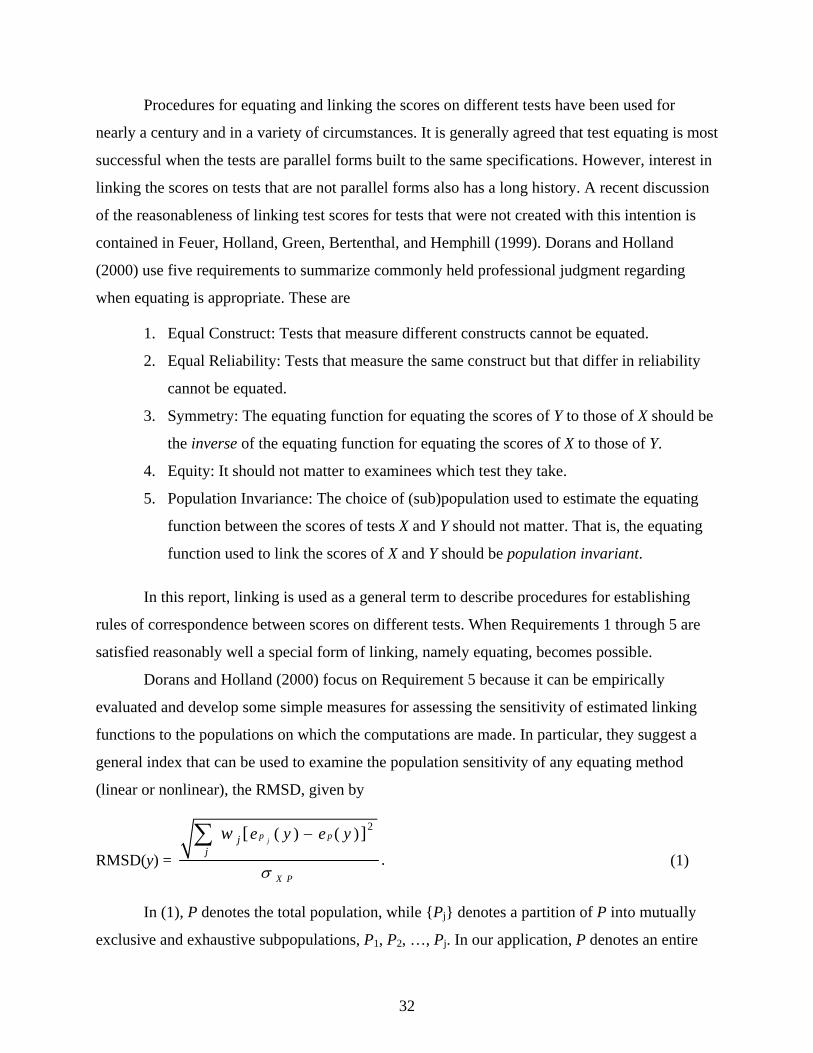
Dorans and Holland (2000) focus on Requirement 5 because it can be empirically

evaluated and develop some simple measures for assessing the sensitivity of estimated linking

functions to the populations on which the computations are made. In particular, they suggest a

general index that can be used to examine the population sensitivity of any equating method

(linear or nonlinear), the RMSD, given by

RMSD(y) =

2( ) ( ).

[ ]jp p

X P

jj

e y e yw

σ

−∑ (1)

In (1), P denotes the total population, while {Pj} denotes a partition of P into mutually

exclusive and exhaustive subpopulations, P1, P2, …, Pj. In our application, P denotes an entire

32

test administration, while the Pj’s are defined by gender or ethnicity, etc. (These subpopulations

are defined more carefully below.) Furthermore, in (1) wj is the weight given to subpopulation Pj.

We will discuss our choice of weights later. The linking function from test Y to test X, computed

for the whole population, is eP(y), and for the subpopulation Pj this linking function is ePj(y).

Finally, in (1), σXP denotes the standard deviation of X-scores in P.

REMSD, a summary measure of RMSD(y), can be obtained by averaging over the

distribution of Y in P before taking the square root in RMSD(y).

In addition to RMSD and REMSD, Dorans and Holland (2000) suggest a special case

that arises when the linking functions are all linear and parallel (with the same slope). In that

case their RMSD measure does not depend on y and may be reexpressed as

RMSD (y) = REMSD = 2[( ) ( )]j jX X Y Yj

j X Yw

μ μ μ μσ σ− −

−∑ P P P P

P P. (2)

In (2), , , ,j jX X Y Yμ μ μ μP P P P denote the means of X and Y on the Pj’s and P. The virtue of

the simplified formula for RMSD is that it is easy to calculate and does not require any actual

score linking. We will use the simplified version of RMSD in this paper in order to compare

several types of linking for some LSAT subpopulations. Some of these links are between parallel

test sections (equating), and some are links between sections that differ considerably from

parallelism.

In their paper, Dorans and Holland (2000) use the relative proportion of a subpopulation

in the total population as its weight, but this is arbitrary. This approach is satisfactory when the

subpopulations are similar in size, but it becomes a problem when one subpopulation is very

small. We decided to use both proportional as well as equal subpopulation weights in the RMSD

calculation. Equal weights are included on the grounds that if a subpopulation is identified as

interesting enough to be included in the comparison, then it deserves to contribute equally to the

results.

We follow Dorans and Holland (2000) and report RMSD values times 100 so that they

are interpretable as percents of a standard deviation.

We should emphasize that these linkages are not actual operational ones, but rather they

provide opportunities for studying links of various sorts that arise in a specific testing program.

Many testing programs provide opportunities for adding to our knowledge about the factors that

33

influence the equatability of tests, and this paper is an example of exploiting these opportunities

in a specific case, the LSAT. We hope that this will encourage others to examine the linking

opportunities in other testing programs and use these opportunities to add to our knowledge

about test equating and linking.

Test Data

The LSAT consists of five 35-minute sections of multiple-choice questions, four of

which contribute to the examinee's score. The scored sections include one analytical reasoning

section (AR), two logical reasoning sections (LA & LB) and one reading comprehension section

(RC). The LSAT is a rights-only scored test; no points are subtracted for wrong responses. Only a

single score is reported for the LSAT.

The current study used operational test data from three LSAT administrations (from three

different years), each of which had over 40,000 examinees, to evaluate the population invariance

of various equatings and linkings using the simplified RMSD measure mentioned earlier. Each

test form used in an administration had two versions: a main form (M) and a shuffled form (S)

that were taken by spiraled samples. These two forms had the same items, but the sections were

in different orders. These test data provide us two different types of data collection designs that

we used for linking. The two spiraled samples taking the M or S forms give us an equivalent

groups design. If we ignore the effect of section order and pool the two forms together, we have

a single group design for linking sections to each other, because every examinee takes every

section. Similarly, if we treat the M and S forms as different, then each spiraled sample gives us

a single group design for linking the section scores together. We made use of all of these types of

designs in our analysis.

Examinee Subpopulations

The subpopulations of interest are defined by examinees’ gender (male and female),

ethnic background (Asian, Black, Hispanic, White, and Other), geographic region, whether the

examinees had applied to law school (yes or no), and law school admission status. As Figure 1

shows, geographic regions divide examinees into eight subgroups: northwest and far west

(including examinees from Alaska and Hawaii), midwest and mountain west, south central,

southeast, midsouth, great lakes, New England and northeast, Canada, and other countries. Law

school admission status defines four subpopulations: examinees who matriculated, examinees

34

who were admitted, examinees whose applications were rejected, and examinees who did not

apply.

Figure 1. Examinee subpopulations by geographic regions.

Equating and Linking Designs

Data sets from three different test administrations afforded us opportunities to evaluate

the population invariance of equating and linking functions in a variety of settings. We started

out with the setting that meets the five equating requirements of Dorans and Holland (2000)

fairly well: equating the main form total score and section scores to their shuffled form

counterparts within each test administration. This setting allows us to establish a baseline for the

Dorans and Holland measure of population sensitivity. As explained previously in the test data

35

section, the main form and shuffled form contained the same items. They only differed in their

section order. Under normal testing conditions there are no significant section order effects

(context effects), and since the tests or sections being equating are parallel, in this case, we

expect small differences between the equating functions computed on different subpopulations.

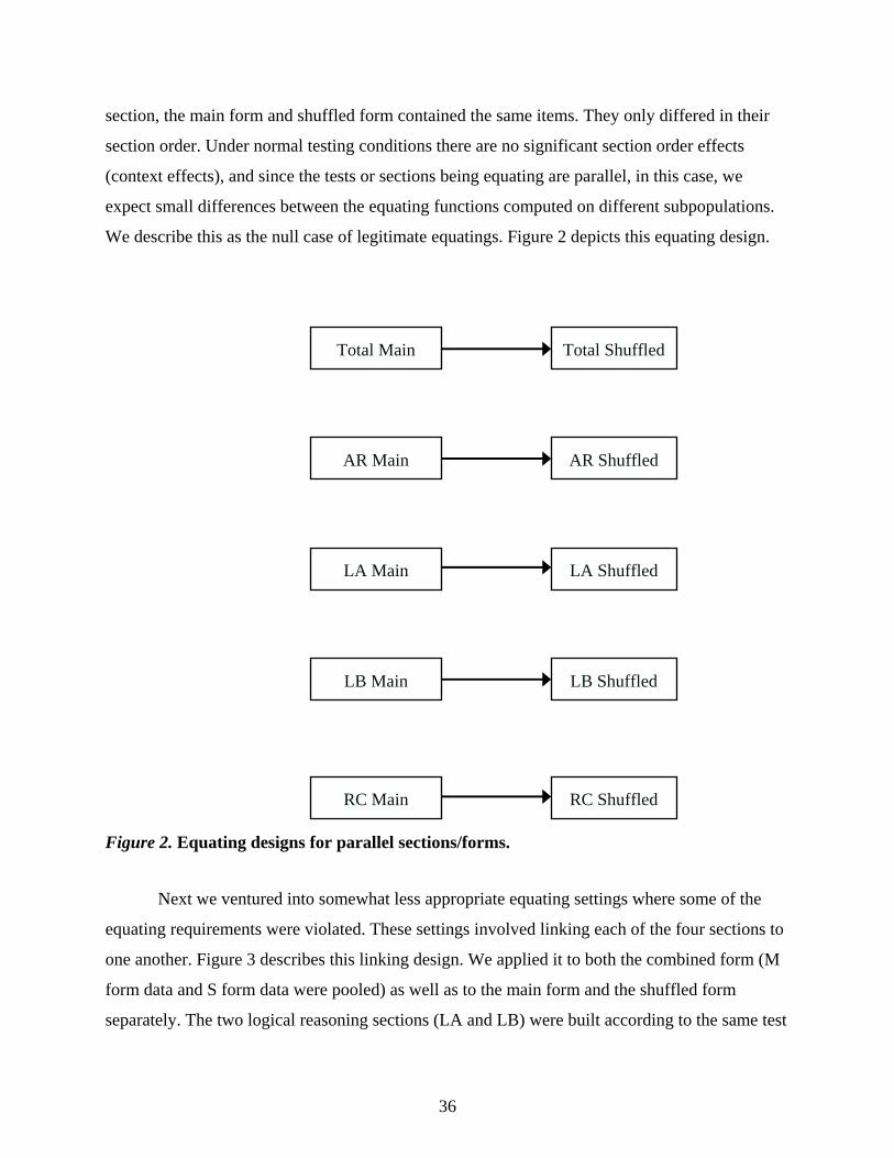
We describe this as the null case of legitimate equatings. Figure 2 depicts this equating design.

Total Main Total Shuffled

Figure 2. Equating designs for parallel sections/forms.

Next we ventured into somewhat less appropriate equating settings where some of the

equating requirements were violated. These settings involved linking each of the four sections to

one another. Figure 3 describes this linking design. We applied it to both the combined form (M

form data and S form data were pooled) as well as to the main form and the shuffled form

separately. The two logical reasoning sections (LA and LB) were built according to the same test

AR Main

LA Main

LB Main

RC Main

AR Shuffled

LA Shuffled

LB Shuffled

RC Shuffled

36

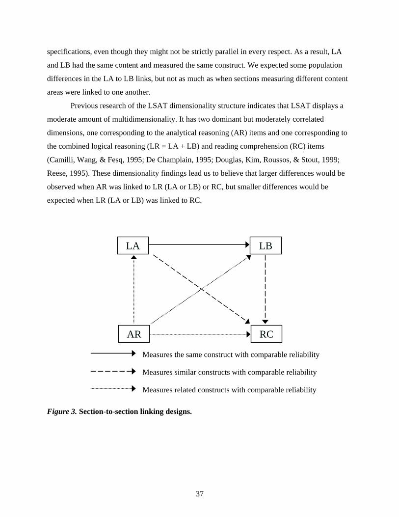
specifications, even though they might not be strictly parallel in every respect. As a result, LA

and LB had the same content and measured the same construct. We expected some population

differences in the LA to LB links, but not as much as when sections measuring different content

areas were linked to one another.

Previous research of the LSAT dimensionality structure indicates that LSAT displays a

moderate amount of multidimensionality. It has two dominant but moderately correlated

dimensions, one corresponding to the analytical reasoning (AR) items and one corresponding to

the combined logical reasoning (LR = LA + LB) and reading comprehension (RC) items

(Camilli, Wang, & Fesq, 1995; De Champlain, 1995; Douglas, Kim, Roussos, & Stout, 1999;

Reese, 1995). These dimensionality findings lead us to believe that larger differences would be

observed when AR was linked to LR (LA or LB) or RC, but smaller differences would be

expected when LR (LA or LB) was linked to RC.

LA LB

AR RC

Measures similar constructs with comparable reliability

Measures the same construct with comparable reliability

Measures related constructs with comparable reliability

Figure 3. Section-to-section linking designs.

37

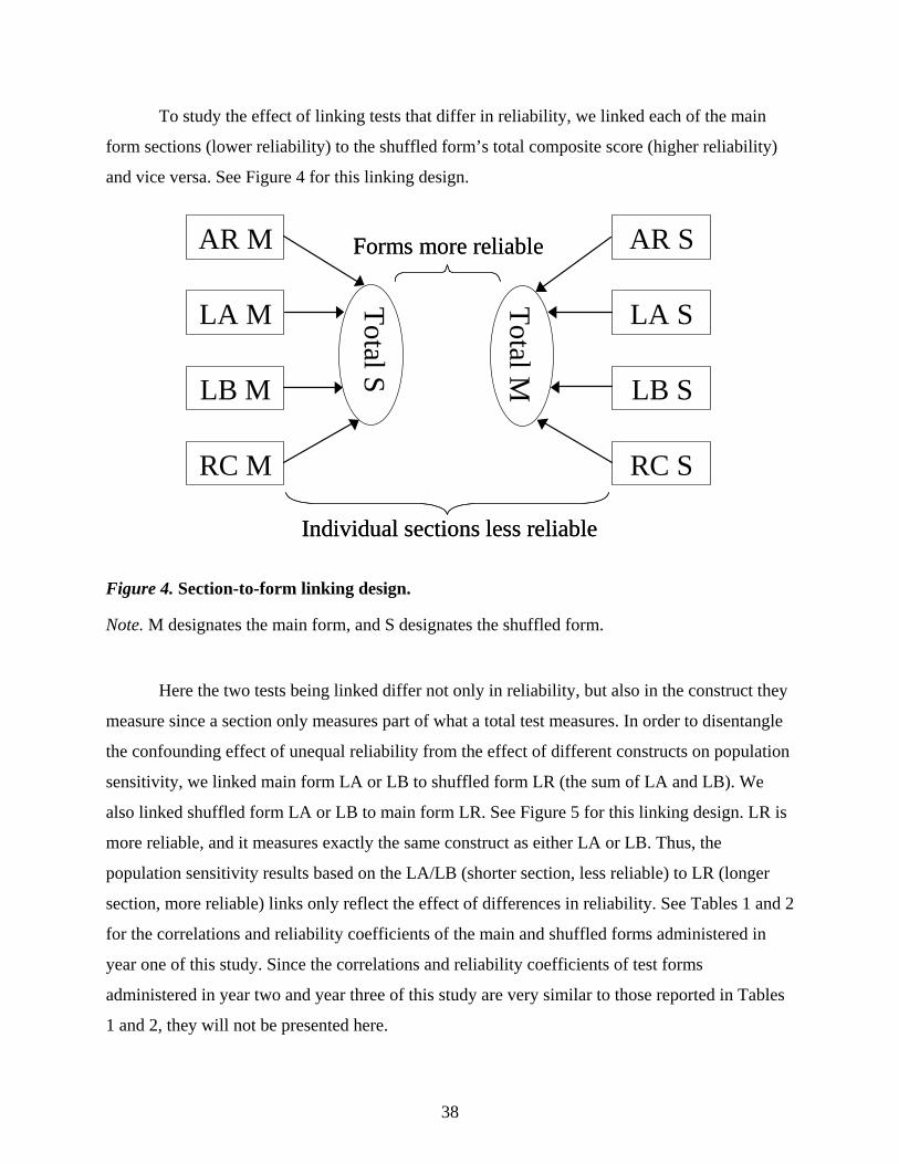
To study the effect of linking tests that differ in reliability, we linked each of the main

form sections (lower reliability) to the shuffled form’s total composite score (higher reliability)

and vice versa. See Figure 4 for this linking design.

AR M

LA M

LB M

RC M

AR S

LA S

LB S

RC S

Total S

Forms more reliableForms more reliable

Individual sections less reliableIndividual sections less reliable

Total M

Figure 4. Section-to-form linking design.

Note. M designates the main form, and S designates the shuffled form.

Here the two tests being linked differ not only in reliability, but also in the construct they

measure since a section only measures part of what a total test measures. In order to disentangle

the confounding effect of unequal reliability from the effect of different constructs on population

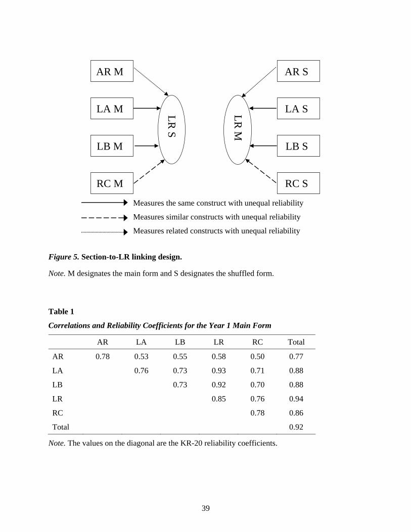
sensitivity, we linked main form LA or LB to shuffled form LR (the sum of LA and LB). We

also linked shuffled form LA or LB to main form LR. See Figure 5 for this linking design. LR is

more reliable, and it measures exactly the same construct as either LA or LB. Thus, the

population sensitivity results based on the LA/LB (shorter section, less reliable) to LR (longer

section, more reliable) links only reflect the effect of differences in reliability. See Tables 1 and 2

for the correlations and reliability coefficients of the main and shuffled forms administered in

year one of this study. Since the correlations and reliability coefficients of test forms

administered in year two and year three of this study are very similar to those reported in Tables

1 and 2, they will not be presented here.

38

AR M

LA M

LB M

RC M

AR S

LA S

LB S

RC S LR

M

LR S

Measures the same construct with unequal reliability

Measures similar constructs with unequal reliability

Measures related constructs with unequal reliability

Figure 5. Section-to-LR linking design.

Note. M designates the main form and S designates the shuffled form.

Table 1

Correlations and Reliability Coefficients for the Year 1 Main Form

AR LA LB LR RC Total

AR 0.78 0.53 0.55 0.58 0.50 0.77

LA 0.76 0.73 0.93 0.71 0.88

LB 0.73 0.92 0.70 0.88

LR 0.85 0.76 0.94

RC 0.78 0.86

Total 0.92

Note. The values on the diagonal are the KR-20 reliability coefficients.

39

Table 2

Correlations and Reliability Coefficients for the Year 1 Shuffled Form

AR LA LB LR RC Total

AR 0.78 0.52 0.55 0.58 0.51 0.76

LA 0.76 0.73 0.94 0.72 0.88

LB 0.73 0.93 0.71 0.88

LR 0.85 0.77 0.94

RC 0.78 0.87

Total 0.92

Note. The values on the diagonal are the KR-20 reliability coefficients.

In summary, the four designs described here have allowed us to examine within each test

administration the population dependence of the equating/linking functions for subpopulations

based on gender, ethnicity, geographic region, whether examinees applied to law school or not,

and their law school admission status. These equating/linking designs were repeated with three

test forms that were administered in three different years.

As mentioned earlier, proportional as well as equal group weights were used for the

RMSD measures. All of the subpopulation information was provided by examinees, and

examinees who did not provide subpopulation information were excluded from our study. We

have collapsed some subpopulation categories to make the sample sizes more reasonable.

Results

In this section, we report RMSD results based on three test administrations (one

administration per year) for a variety of linking functions across the LSAT subpopulations

defined by gender, ethnicity, geographic region, whether examinees applied to law school, and

their law school admission status.

Linking Parallel Forms

The main form total and section scores were linked to their parallel shuffled form total

and section scores (See Figure 2 for the design). There were five linkages for each defined LSAT

subpopulation: main form total to shuffled form total, main form AR to shuffled form AR, main

40

form LA to shuffled form LA, main form LB to shuffled form LB, and main form RC to shuffled

form RC. Since the main and the shuffled forms contained the same items, they were considered

parallel forms, so these linkings are essentially equatings. Under normal testing conditions there

are no significant section order effects (context effects), so we expect very small differences in

the subpopulation linkages between these two forms.

Figure 6 displays the equal weight RMSD results for the five subpopulation variables.

The vertical axis is the RMSD value expressed in percent of a standard deviation, and the

horizontal axis shows the equating linkages and testing year. Let us focus on the equating of the

main form total score (TS M) to the shuffled form total score (TS S), the block of three columns

on the far right of Figure 6. RMSD values for this linkage across three testing years range from

0.2% to 4.1%. Gender, whether examinees applied to law school and examinee’s law school

admission status exhibit little population dependence with RMSD values ranging from 0.2% to

1.0%. The RMSD values for ethnicity and geographic region are somewhat larger (2.0% to

4.1%). Similarly, across the four parallel section linkages (the four remaining blocks of columns

moving from right to left), geographic region and ethnicity display somewhat larger RMSD

values, ranging from 1.5% to 3.5%. In general, these RMSD values indicate very little

population dependence on these equating functions.

Figure 7 shows the RMSD results for the same parallel linkages using proportional

subpopulation weights. The RMSDs tend to be a bit smaller than those based on equal group

weights, and the trend of little population dependence is quite consistent.

Table A1 presents the RMSD values used to produce Figure 6 and Figure 7.

These results support our expectations that in equating situations, linking functions are

quite similar across the subpopulations defined by gender, ethnicity, geographic region,

application to law school, and law school admission status.

Even though we anticipated that the RMSD values would be small for these equatings, it

might be expected that equating each of the main form section scores to its shuffled form

counterpart section scores would yield somewhat higher RMSD values than would the total score

equating linkage because of the higher reliability of the total score (0.92) than the section scores

(0.73 – 0.78). However, this did not happen. Instead, the RMSD values from the section linkages

are quite comparable to those from the total score linkages. This might suggest that for parallel

measures the actual amount of reliability is not a significant factor if the two tests have sufficient

41

reliability. This is a result worth examining in other data sets. It is hard to say precisely how much

reliability is enough for equatings to be population invariant. Dorans (2004b) discussed this point

in more detail and related it to the bound on RMSD given in Dorans and Holland (2000). See

Tables 1 and 2 for correlations and reliabilities of the main and the shuffled forms administered in

the first year. These correlations and reliabilities are very similar to those of the other two forms.

These RMSD results from parallel form/section linkages will be used as benchmark

values to evaluate other linkages that violated some or all of the five equating requirements of

Dorans and Holland (2000).

Section Linkages of Varying Content/Construct

In this section, we will report population invariance results of linking each of the four

LSAT section scores to one another. The linkings were performed for the combined form data

(main form and shuffled form data were pooled together), as well as for the main and the

shuffled form data separately (see Figure 3 for the design). A total of six linkages were

performed for each case. The key difference between these linking functions and the baseline

cases described above is that the sections being linked don’t necessarily measure the same

construct. The four sections do have comparable KR-20 reliabilities (0.73 – 0.78; see Tables 1

and 2). Since the results are similar across the combined form, the main form and the shuffled

form, only the combined form results will be presented here.

Figure 8 depicts the RMSD results of linking section scores using equal group weights. A

quick glance at Figure 8 reveals at least two important patterns. First, any linkage containing AR

resulted in the least invariant linking functions. This is expected since the correlations between

AR and LA, AR and LB, and AR and RC are only in the 0.50 range. Moreover, this result is

consistent with the previously mentioned dimensionality analyses performed on the LSAT data.

The LSAT has two dominant but moderately correlated dimensions, one corresponding to the

AR items and one corresponding to the combined LR and RC items. As expected, the LA to LB

and LB to RC linkages, in general, exhibited smaller population dependence (with the exception

of the third year result of LB to RC link). We expected to see smaller RMSD values for these

linkages because LR and RC are more highly correlated and both item types have been shown to

load on the same underlying factor.

42

-202468

1012141618202224

1 2 3 1 2 3 1 2 3 1 2 3 1 2 3

AR -> LA AR -> LB AR -> RC LA -> LB LA -> RCLINKING

RM

SD (%

)Applied to Law School?Ethnicity

GenderGeographic Region

Admission Status

1 2 3 1 2 3 1 2 3 1 2 3 1 2 3AR M => AR S LA M => LA S LB M => LB S RC M => RC S TS M => TS S

LINKING

Figure 6. Form-to-form linkings across three LSAT test administrations using equal

weights and excluding all missing data.

-202468

1012141618202224

1 2 3 1 2 3 1 2 3 1 2 3 1 2 3

AR->LA

AR->LA

AR ->LA

AR->LB

AR->LB

AR ->LB

AR->

RC

AR->RC

AR ->RC

LA->LB

LA->LB

LA ->LB

LA->RC

LA->

RC

LA->RCLINKING

RM

SD (%

)

Applied to Law School?

Ethnicity

Gender

Geographic Region

Admission Status

1 2 3 1 2 3 1 2 3 1 2 3 1 2 3AR M => AR S LA M => LA S LB M => LB S RC M => RC S TS M => TS S

LINKING Figure 7. Form-to-form linkings across three LSAT test administrations using proportional

weights and excluding all missing data.

43

The second pattern in Figure 8 reflects the effect of ethnicity. Most ethnic subpopulation

linkages exhibit large population sensitivity, with RMSD values ranging from 7.9% to 19.5%

(with some exceptions in the LA to LB, LA to RC, and LB to RC linkages), indicating that the

linking functions for the ethnicity subpopulations differ substantially from that of the total

population. These RMSD values are well above our benchmark values (the largest benchmark

RMSD is 4.1%), and they reinforce the finding that linking two tests (in this case two sections

like AR and LA or AR and RC) that measure different constructs may result in substantial

population dependence. As described before, the RMSD results from parallel form/section

linkages are used as benchmark values.

For linkages involving AR (with the exception of AR to RC), gender exhibits larger than

the benchmark RMSD values, ranging from 6.5% to 11.8%. Any linkages involving AR yield

slightly to moderately larger than the benchmark RMSD values (4.5% to 7.6%) across the

subpopulations of law school admission status.

Figure 9 shows the RMSD results of section linkages using proportional group weights.

As with the equal group weights case, linkages involving AR still exhibit less population

invariance than other linkages across subpopulations defined by ethnicity, gender, and

examinee’s law school admission status. But the magnitude of the RMSD values is diminished.

While linkages involving AR still tend to be more population dependent across the ethnic

subpopulations, their RMSD values are not as prominent as in the equal group weights case

(6.2% to 13.1% vs. 7.9% to 19.5%).

See Table A2 for the RMSD values used to produce Figure 8 and Figure 9.

Linking Less Reliable Section Scores to More Reliable Total Scores

One area that we wanted to explore with these data is the population sensitivity of links

between two measures that are not equally reliable. To study this, we linked each of the four main

form section scores (AR M, LA M, LB M, and RC M) to the shuffled form total score (TS S). We

also linked each of the four shuffled form section scores to the main form total score as a cross-

validation check. Since the results are similar, we will only report the RMSD values for linking the

main form section scores to the shuffled form total score.

The block of three columns on the far right of Figure 10 shows the benchmark values for

equating equally reliable parallel total forms using equal weights from Figure 6. (As Figure 6

shows, the benchmark values for linking equally reliable parallel sections are similar.) The other

44

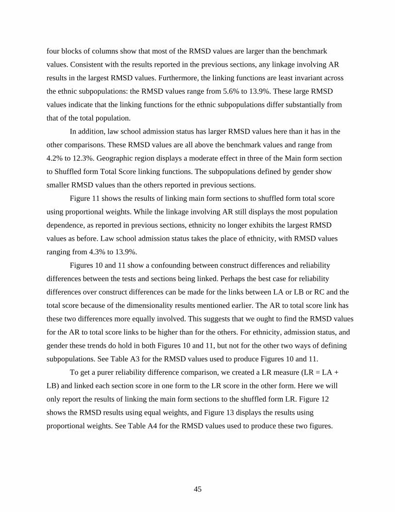
four blocks of columns show that most of the RMSD values are larger than the benchmark

values. Consistent with the results reported in the previous sections, any linkage involving AR

results in the largest RMSD values. Furthermore, the linking functions are least invariant across

the ethnic subpopulations: the RMSD values range from 5.6% to 13.9%. These large RMSD

values indicate that the linking functions for the ethnic subpopulations differ substantially from

that of the total population.

In addition, law school admission status has larger RMSD values here than it has in the

other comparisons. These RMSD values are all above the benchmark values and range from

4.2% to 12.3%. Geographic region displays a moderate effect in three of the Main form section

to Shuffled form Total Score linking functions. The subpopulations defined by gender show

smaller RMSD values than the others reported in previous sections.

Figure 11 shows the results of linking main form sections to shuffled form total score

using proportional weights. While the linkage involving AR still displays the most population

dependence, as reported in previous sections, ethnicity no longer exhibits the largest RMSD

values as before. Law school admission status takes the place of ethnicity, with RMSD values

ranging from 4.3% to 13.9%.

Figures 10 and 11 show a confounding between construct differences and reliability

differences between the tests and sections being linked. Perhaps the best case for reliability

differences over construct differences can be made for the links between LA or LB or RC and the

total score because of the dimensionality results mentioned earlier. The AR to total score link has

these two differences more equally involved. This suggests that we ought to find the RMSD values

for the AR to total score links to be higher than for the others. For ethnicity, admission status, and

gender these trends do hold in both Figures 10 and 11, but not for the other two ways of defining

subpopulations. See Table A3 for the RMSD values used to produce Figures 10 and 11.

To get a purer reliability difference comparison, we created a LR measure (LR = LA +

LB) and linked each section score in one form to the LR score in the other form. Here we will

only report the results of linking the main form sections to the shuffled form LR. Figure 12

shows the RMSD results using equal weights, and Figure 13 displays the results using

proportional weights. See Table A4 for the RMSD values used to produce these two figures.

45

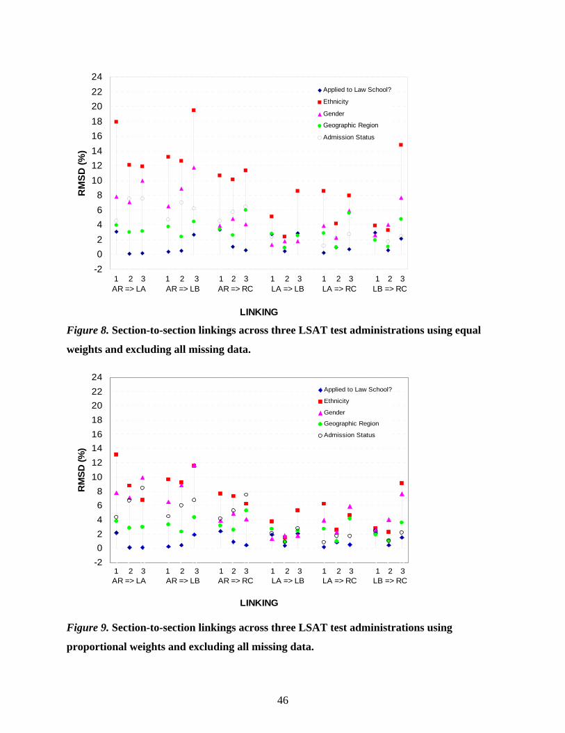
-202468

1012141618202224

1 2 3 1 2 3 1 2 3 1 2 3 1 2 3 1 2 3

AR -> LA AR -> LB AR -> RC LA -> LB LA -> RC LB ->RC

LINKING

RM

SD (%

)Applied to Law School?

Ethnicity

Gender

Geographic Region

Admission Status

1 2 3 1 2 3 1 2 3 1 2 3 1 2 3 1 2 3AR => LA AR => LB AR => RC LA => LB LA => RC LB => RC

Figure 8. Section-to-section linkings across three LSAT test administrations using equal

weights and excluding all missing data.

-202468

1012141618202224

1 2 3 1 2 3 1 2 3 1 2 3 1 2 3 1 2 3

AR->LA

AR->LA

AR -> LA

AR->LB

AR->LB

AR -> LB

AR->

RC

AR->

RC

AR -> RC

LA->LB

LA->LB

LA ->LB

LA->

RC

LA->

RC

LA ->RC

LB->

RC

LB->

RC

LB->

RCLINKING

RM

SD (%

)

Applied to Law School?

Ethnicity

Gender

Geographic Region

Admission Status

1 2 3 1 2 3 1 2 3 1 2 3 1 2 3 1 2 3AR => LA AR => LB AR => RC LA => LB LA => RC LB => RC

Figure 9. Section-to-section linkings across three LSAT test administrations using

proportional weights and excluding all missing data.

46

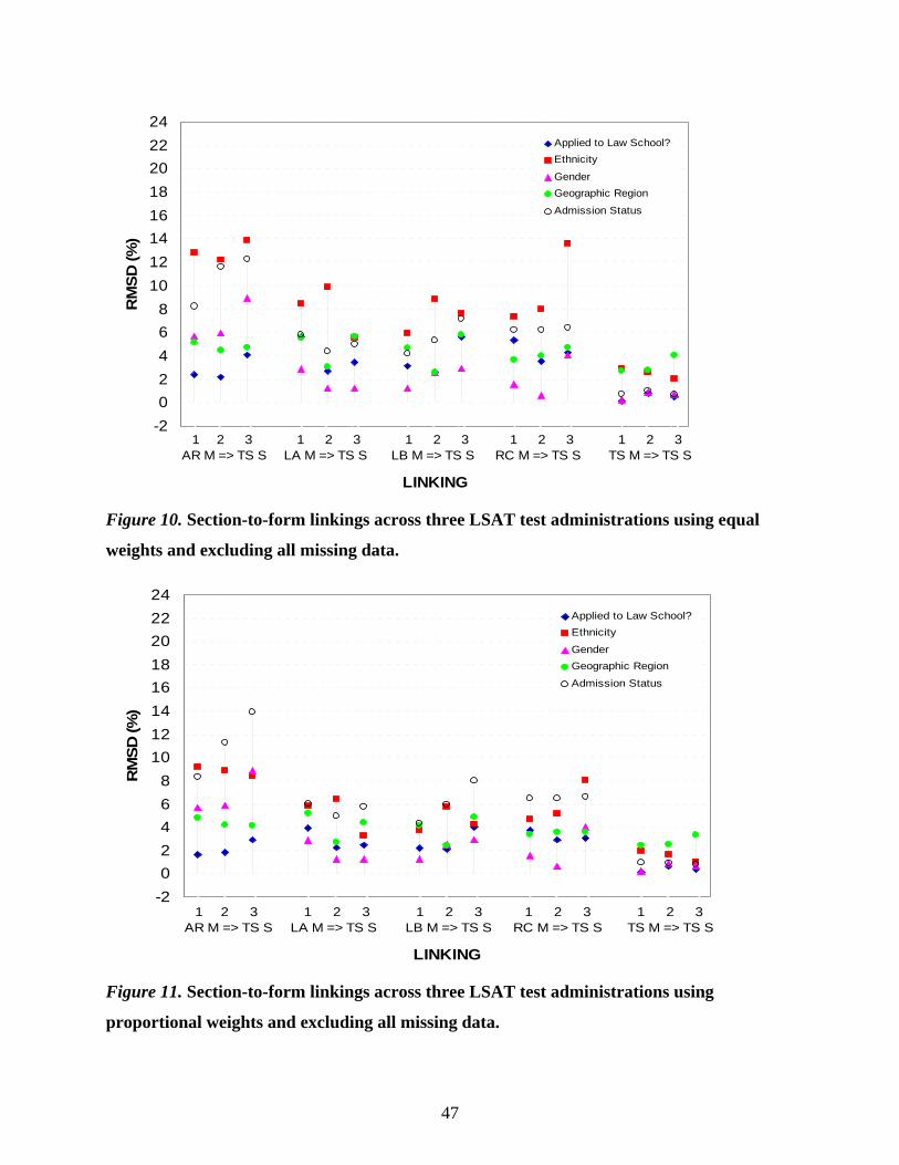
-202468

1012141618202224

1 2 3 1 2 3 1 2 3 1 2 3 1 2 3

AR -> LA AR -> LB AR -> RC LA -> LB LA -> RCLINKING

RM

SD (%

)Applied to Law School?Ethnicity

GenderGeographic Region

Admission Status

1 2 3 1 2 3 1 2 3 1 2 3 1 2 3AR M => TS S LA M => TS S LB M => TS S RC M => TS S TS M => TS S

LINKING

Figure 10. Section-to-form linkings across three LSAT test administrations using equal

weights and excluding all missing data.

-202468

1012141618202224

1 2 3 1 2 3 1 2 3 1 2 3 1 2 3

AR->LA

AR->LA

AR ->LA

AR->LB

AR->LB

AR ->LB

AR->

RC

AR->

RC

AR ->RC

LA->LB

LA->LB

LA ->LB

LA->

RC

LA->

RC

LA->

RCLINKING

RM

SD (%

)

Applied to Law School?Ethnicity

GenderGeographic Region

Admission Status

1 2 3 1 2 3 1 2 3 1 2 3 1 2 3AR M => TS S LA M => TS S LB M => TS S RC M => TS S TS M => TS S

LINKING

Figure 11. Section-to-form linkings across three LSAT test administrations using

proportional weights and excluding all missing data.

47

-202468

1012141618202224

1 2 3 1 2 3 1 2 3 1 2 3 1 2 3

AR -> LA AR -> LB AR -> RC LA -> LB LA -> RCLINKING

RM

SD (%

)Applied to Law School?Ethnicity

GenderGeographic Region

Admission Status

1 2 3 1 2 3 1 2 3 1 2 3 1 2 3AR M => LR S LA M => LR S LB M => LR S RC M => LR S TS M => TS S

LINKING

Figure 12. Section-to-LR linkings across three LSAT test administrations using equal

weights and excluding all missing data.

-202468

1012141618202224

1 2 3 1 2 3 1 2 3 1 2 3 1 2 3

AR->LA

AR->LA

AR ->LA

AR->LB

AR->LB

AR ->LB

AR->

RC

AR->

RC

AR ->RC

LA->LB

LA->LB

LA ->LB

LA->

RC

LA->

RC

LA->

RCLINKING

RM

SD (%

)

Applied to Law School?Ethnicity

GenderGeographic Region

Admission Status

1 2 3 1 2 3 1 2 3 1 2 3 1 2 3AR M => LR S LA M => LR S LB M => LR S RC M => LR S TS M => TS S

LINKING

Figure 13. Section-to-LR linkings across three LSAT test administrations using

proportional weights and excluding all missing data.

48

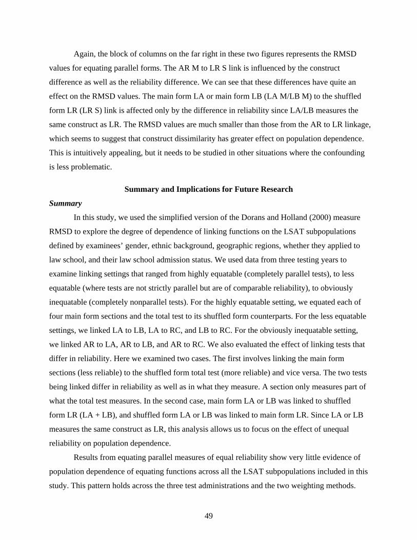
Again, the block of columns on the far right in these two figures represents the RMSD

values for equating parallel forms. The AR M to LR S link is influenced by the construct

difference as well as the reliability difference. We can see that these differences have quite an

effect on the RMSD values. The main form LA or main form LB (LA M/LB M) to the shuffled

form LR (LR S) link is affected only by the difference in reliability since LA/LB measures the

same construct as LR. The RMSD values are much smaller than those from the AR to LR linkage,

which seems to suggest that construct dissimilarity has greater effect on population dependence.

This is intuitively appealing, but it needs to be studied in other situations where the confounding

is less problematic.

Summary and Implications for Future Research

Summary

In this study, we used the simplified version of the Dorans and Holland (2000) measure

RMSD to explore the degree of dependence of linking functions on the LSAT subpopulations

defined by examinees’ gender, ethnic background, geographic regions, whether they applied to

law school, and their law school admission status. We used data from three testing years to

examine linking settings that ranged from highly equatable (completely parallel tests), to less

equatable (where tests are not strictly parallel but are of comparable reliability), to obviously

inequatable (completely nonparallel tests). For the highly equatable setting, we equated each of

four main form sections and the total test to its shuffled form counterparts. For the less equatable

settings, we linked LA to LB, LA to RC, and LB to RC. For the obviously inequatable setting,

we linked AR to LA, AR to LB, and AR to RC. We also evaluated the effect of linking tests that

differ in reliability. Here we examined two cases. The first involves linking the main form

sections (less reliable) to the shuffled form total test (more reliable) and vice versa. The two tests

being linked differ in reliability as well as in what they measure. A section only measures part of

what the total test measures. In the second case, main form LA or LB was linked to shuffled

form LR (LA + LB), and shuffled form LA or LB was linked to main form LR. Since LA or LB

measures the same construct as LR, this analysis allows us to focus on the effect of unequal

reliability on population dependence.

Results from equating parallel measures of equal reliability show very little evidence of

population dependence of equating functions across all the LSAT subpopulations included in this

study. This pattern holds across the three test administrations and the two weighting methods.

49

The fact that RMSD values from equating parallel sections are comparable to those from

equating parallel total forms seems to suggest that for equating parallel measures, the actual

amount of reliability does not seem to be a significant factor if the tests have sufficient

reliability. Since it is difficult to prescribe precisely how much reliability is needed for equatings

to be population invariant, it would be useful for future research to investigate and document a

wide range of equating conditions and reliabilities that seem to produce invariant results.

Consistent with our expectations, linking two tests that are not strictly parallel but measure

the same construct resulted in smaller population sensitivity than linking two nonparallel tests that

do not measure the same thing. Linking two tests that measure different things will lead to

substantial population dependence as measured by RMSD. Proportional weights seem to diminish

the RMSD values that are based on equal weights. Linking functions that measure different

constructs are the least invariant across the ethnic subpopulations. This phenomenon is

particularly noticeable with equal group weights. With proportional group weights, admission

status and gender seem to yield RMSD values that become noticeably less invariant.

Unequal reliability has an effect on population dependence of linking functions, but it

appears to be smaller than the effect of linking two tests that measure different constructs. Once

again, future research should look into how different amounts of unequal reliability affect

population dependence.

Readers should keep this in mind when evaluating the results presented in this study. The

sample sizes of the subpopulations used her are much smaller than those used in the Dorans and

Holland paper (2000). Naturally, the results reported here will reflect some of the sampling

variability, but we did not examine this factor in the present study. The sampling variability of the

RMSD results across the three test administrations indicates the need to get good measures of

variability for the Dorans and Holland indices. This is a useful topic for future research.

Implications for Future Research

In this study, we concentrated on the simplest version of the RMSD measure based on the

parallel-linear equating model. It would be helpful to see if using more complicated, nonlinear

equating functions, such as kernel equating, would give very different results. If they did, this

would indicate a limitation to the use of the simple version of RMSD. If they did not, this fact

would allow population sensitivity studies to be carried out without performing actual equatings.

50

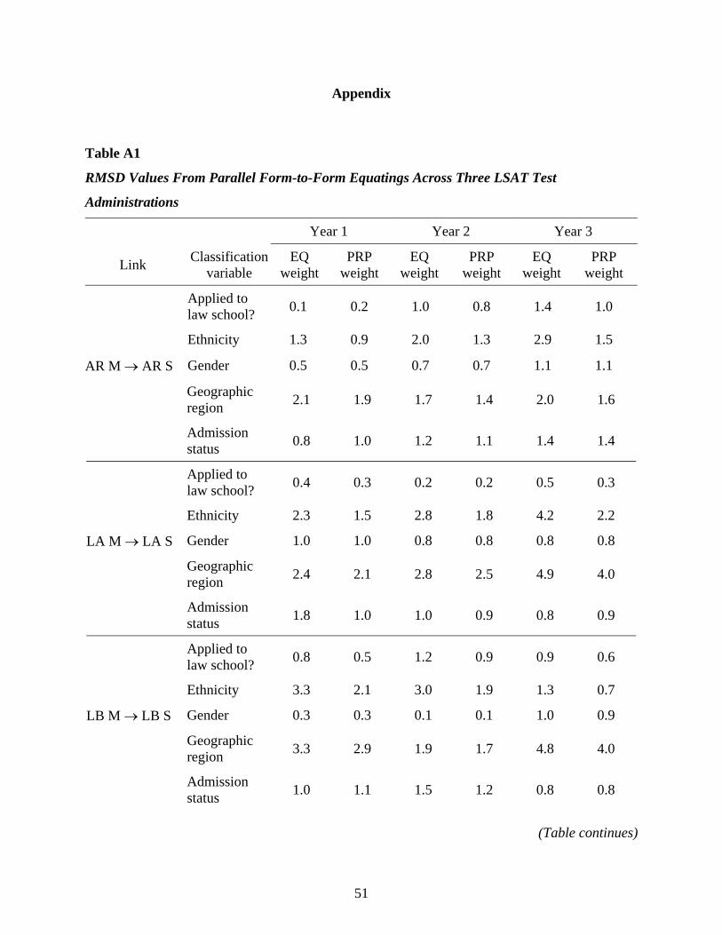
Appendix

Table A1

RMSD Values From Parallel Form-to-Form Equatings Across Three LSAT Test

Administrations

Year 1 Year 2 Year 3

Link Classification variable

EQ weight

PRP weight

EQ weight

PRP weight

EQ weight

PRP weight

Applied to law school? 0.1 0.2 1.0 0.8 1.4 1.0

Ethnicity 1.3 0.9 2.0 1.3 2.9 1.5

AR M → AR S Gender 0.5 0.5 0.7 0.7 1.1 1.1

Geographic region 2.1 1.9 1.7 1.4 2.0 1.6

Admission status 0.8 1.0 1.2 1.1 1.4 1.4

Applied to law school? 0.4 0.3 0.2 0.2 0.5 0.3

Ethnicity 2.3 1.5 2.8 1.8 4.2 2.2

LA M → LA S Gender 1.0 1.0 0.8 0.8 0.8 0.8

Geographic region 2.4 2.1 2.8 2.5 4.9 4.0

Admission status 1.8 1.0 1.0 0.9 0.8 0.9

Applied to law school? 0.8 0.5 1.2 0.9 0.9 0.6

Ethnicity 3.3 2.1 3.0 1.9 1.3 0.7

LB M → LB S Gender 0.3 0.3 0.1 0.1 1.0 0.9

Geographic region 3.3 2.9 1.9 1.7 4.8 4.0

Admission status 1.0 1.1 1.5 1.2 0.8 0.8

(Table continues)

51

Table A1 (continued)

Year 1 Year 2 Year 3

Link Classification variable

EQ weight

PRP weight

EQ weight

PRP weight

EQ weight

PRP weight

Applied to law school? 0.7 0.6 0.5 0.4 0.7 0.5

Ethnicity 3.4 2.4 2.6 1.5 2.0 1.0

RC M → RC S Gender 0.0 0.0 1.5 1.5 0.4 0.4

Geographic region 2.8 2.5 4.0 3.6 3.9 3.3

Admission status 1.0 1.0 0.6 0.7 0.7 0.7

Applied to law school? 0.2 0.2 0.9 0.4 0.5 0.3

Ethnicity 2.9 2.0 2.6 1.5 2.0 1.0

TS M → TS S Gender 0.2 0.2 0.9 1.8 0.7 0.7

Geographic region 2.7 2.5 2.8 0.9 4.1 3.3

Admission status 0.8 1.0 1.0 0.9 0.7 0.8

Table A2

RMSD Values From Section-to-Section Linkings Across Three LSAT Test Administrations

Year 1 Year 2 Year 3

Link Classification variable

EQ weight

PRP weight

EQ weight

PRP weight

EQ weight

PRP weight

Applied to law school? 3.1 2.2 0.1 0.1 0.2 0.1

Ethnicity 17.9 13.1 12.1 8.8 11.8 6.8

AR → LA Gender 7.8 7.8 7.1 7.1 10.0 9.9

Geographic region 3.9 3.8 3.0 2.9 3.2 3.0

Admission status 4.5 4.3 7.6 6.7 7.6 8.4

(Table continues)

52

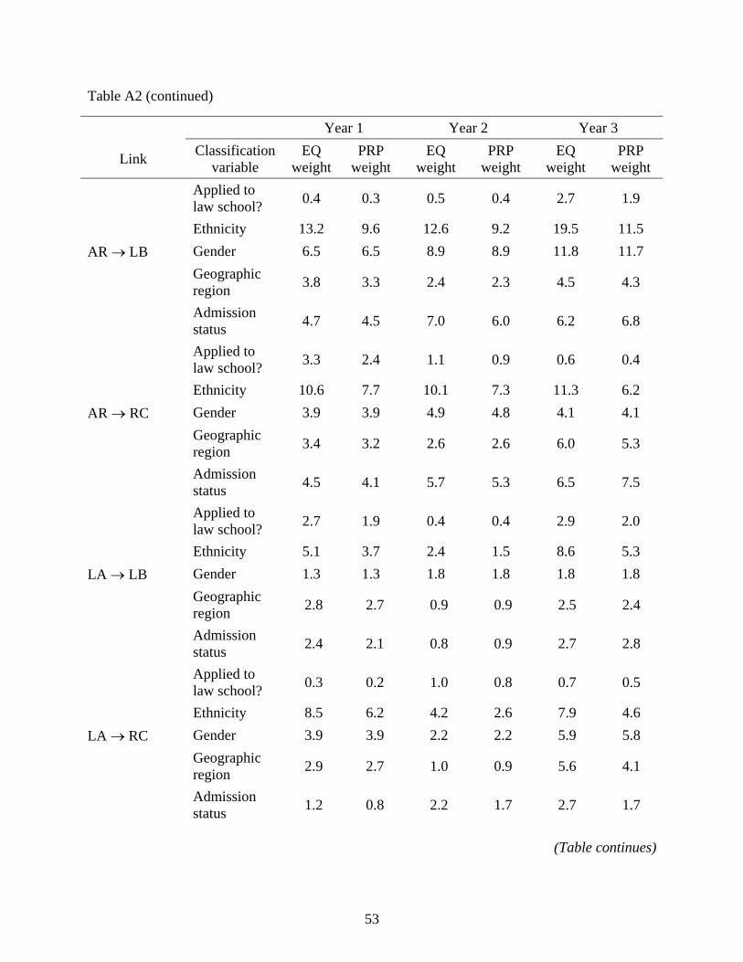
Table A2 (continued)

Year 1 Year 2 Year 3

Link Classification variable

EQ weight

PRP weight

EQ weight

PRP weight

EQ weight

PRP weight

Applied to law school? 0.4 0.3 0.5 0.4 2.7 1.9

Ethnicity 13.2 9.6 12.6 9.2 19.5 11.5 AR → LB Gender 6.5 6.5 8.9 8.9 11.8 11.7

Geographic region 3.8 3.3 2.4 2.3 4.5 4.3

Admission status 4.7 4.5 7.0 6.0 6.2 6.8

Applied to law school? 3.3 2.4 1.1 0.9 0.6 0.4

Ethnicity 10.6 7.7 10.1 7.3 11.3 6.2 AR → RC Gender 3.9 3.9 4.9 4.8 4.1 4.1

Geographic region 3.4 3.2 2.6 2.6 6.0 5.3

Admission status 4.5 4.1 5.7 5.3 6.5 7.5

Applied to law school? 2.7 1.9 0.4 0.4 2.9 2.0

Ethnicity 5.1 3.7 2.4 1.5 8.6 5.3 LA → LB Gender 1.3 1.3 1.8 1.8 1.8 1.8

Geographic region 2.8 2.7 0.9 0.9 2.5 2.4

Admission status 2.4 2.1 0.8 0.9 2.7 2.8

Applied to law school? 0.3 0.2 1.0 0.8 0.7 0.5

Ethnicity 8.5 6.2 4.2 2.6 7.9 4.6 LA → RC Gender 3.9 3.9 2.2 2.2 5.9 5.8

Geographic region 2.9 2.7 1.0 0.9 5.6 4.1

Admission status 1.2 0.8 2.2 1.7 2.7 1.7

(Table continues)

53

Table A2 (continued)

Year 1 Year 2 Year 3

Link Classification variable

EQ weight

PRP weight

EQ weight

PRP weight

EQ weight

PRP weight

Applied to law school? 3.0 2.1 0.6 0.5 2.1 1.5

Ethnicity 3.9 2.8 3.3 2.2 14.8 9.1 LB → RC Gender 2.6 2.6 4.0 4.0 7.7 7.6

Geographic region 1.9 1.9 1.1 1.1 4.8 3.6

Admission status 2.3 2.4 1.7 1.0 2.5 2.2

Table A3

RMSD Values From Section-to-Form Linkings Across Three LSAT Test Administrations

Year 1 Year 2 Year 3

Link Classification variable

EQ weight

PRP weight

EQ weight

PRP weight

EQ weight

PRP weight

Applied to law school? 2.4 1.6 2.2 1.8 4.1 2.9

Ethnicity 12.8 9.2 12.2 8.8 13.9 8.4

AR M → TS S Gender 5.7 5.7 5.9 5.9 8.9 8.8

Geographic region 5.1 4.8 4.5 4.2 4.7 4.1

Admission status 8.2 8.3 11.6 11.3 12.3 13.9

Applied to law school? 5.6 3.9 2.7 2.3 3.4 2.4

Ethnicity 8.5 5.9 9.8 6.4 5.6 3.3

LA M → TS S Gender 2.9 2.8 1.2 1.2 1.2 1.2

Geographic region 5.5 5.2 3.0 2.8 5.7 4.4

Admission status 5.8 6.0 4.4 4.9 5.0 5.8

(Table continues)

54

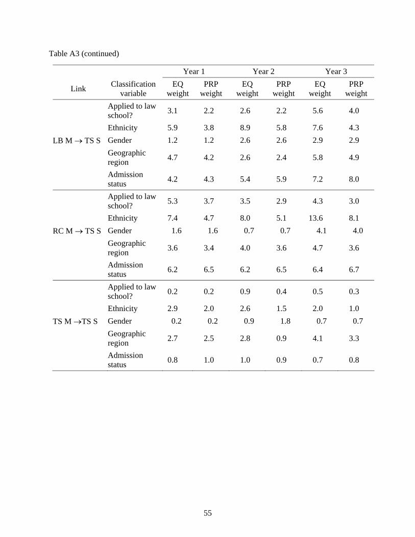
Table A3 (continued)

Year 1 Year 2 Year 3

Link Classification variable

EQ weight

PRP weight

EQ weight

PRP weight

EQ weight

PRP weight

Applied to law school? 3.1 2.2 2.6 2.2 5.6 4.0

Ethnicity 5.9 3.8 8.9 5.8 7.6 4.3 LB M → TS S Gender 1.2 1.2 2.6 2.6 2.9 2.9

Geographic region 4.7 4.2 2.6 2.4 5.8 4.9

Admission status 4.2 4.3 5.4 5.9 7.2 8.0

Applied to law school? 5.3 3.7 3.5 2.9 4.3 3.0

Ethnicity 7.4 4.7 8.0 5.1 13.6 8.1 RC M → TS S Gender 1.6 1.6 0.7 0.7 4.1 4.0

Geographic region 3.6 3.4 4.0 3.6 4.7 3.6

Admission status 6.2 6.5 6.2 6.5 6.4 6.7

Applied to law school? 0.2 0.2 0.9 0.4 0.5 0.3

Ethnicity 2.9 2.0 2.6 1.5 2.0 1.0 TS M →TS S Gender 0.2 0.2 0.9 1.8 0.7 0.7

Geographic region 2.7 2.5 2.8 0.9 4.1 3.3

Admission status 0.8 1.0 1.0 0.9 0.7 0.8

55

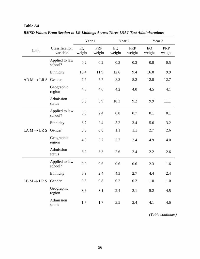
Table A4

RMSD Values From Section-to-LR Linkings Across Three LSAT Test Administrations

Year 1 Year 2 Year 3

Link Classification variable

EQ weight

PRP weight

EQ weight

PRP weight

EQ weight

PRP weight

Applied to law school? 0.2 0.2 0.3 0.3 0.8 0.5

Ethnicity 16.4 11.9 12.6 9.4 16.8 9.9

AR M → LR S Gender 7.7 7.7 8.3 8.2 12.8 12.7

Geographic region 4.8 4.6 4.2 4.0 4.5 4.1

Admission status 6.0 5.9 10.3 9.2 9.9 11.1

Applied to law school? 3.5 2.4 0.8 0.7 0.1 0.1

Ethnicity 3.7 2.4 5.2 3.4 5.6 3.2

LA M → LR S Gender 0.8 0.8 1.1 1.1 2.7 2.6

Geographic region 4.0 3.7 2.7 2.4 4.9 4.0

Admission status 3.2 3.3 2.6 2.4 2.2 2.6

Applied to law school? 0.9 0.6 0.6 0.6 2.3 1.6

Ethnicity 3.9 2.4 4.3 2.7 4.4 2.4

LB M → LR S Gender 0.8 0.8 0.2 0.2 1.0 1.0

Geographic region 3.6 3.1 2.4 2.1 5.2 4.5

Admission status 1.7 1.7 3.5 3.4 4.1 4.6

(Table continues)

56

Table A4 (continued)

Year 1 Year 2 Year 3

Link Classification variable

EQ weight

PRP weight

EQ weight

PRP weight

EQ weight

PRP weight

Applied to law school? 3.2 2.2 1.5 1.3 0.9 0.7

Ethnicity 6.7 4.6 5.0 3.2 13.9 8.2

RC M → LR S Gender 3.6 3.6 3.0 3.0 8.0 7.9

Geographic region 2.6 2.5 3.6 3.3 5.2 3.8

Admission status 3.6 3.7 4.5 4.0 3.9 3.5

Applied to law school? 0.2 0.2 0.9 0.4 0.5 0.3

Ethnicity 2.9 2.0 2.6 1.5 2.0 1.0

TS M → TS S Gender 0.2 0.2 0.9 1.8 0.7 0.7

Geographic region 2.7 2.5 2.8 0.9 4.1 3.3

Admission status 0.8 1.0 1.0 0.9 0.7 0.8

57

Invariance of Score Linkings Across Gender Groups for Forms

of a Testlet-Based CLEP® Examination

Wen-Ling Yang and Rui Gao

ETS, Princeton, NJ

59

Abstract

This study investigates whether the functions that link number-right raw scores to the College-

Level Examination Program® (CLEP®) scaled scores remain invariant over gender groups. Test

data for the 16 testlet-based forms of the CLEP College Algebra exam were used to study linking

invariance. The linking of various test forms to a common reference form is based on the Rasch

model. The equatability indices proposed by Dorans and Holland (2000) were employed to

evaluate the invariance of the linking functions over gender subpopulations. Overall, the linkings

based on the gender groups are very similar to the linkings based on the total group. At various

score levels, differences between subgroups and total group linkings are all smaller than the

difference that will impact the pass/fail decision for CLEP candidates. At the recommended cut

score of 50 on the CLEP scale, due to rounding and for only one form, the linking based on the

male group would pass more candidates than the linking based on the total group. However, only

a rather small portion of the candidate group taking the particular form would be affected.

Key words: Test equating, linking, invariance of linking, equitability

60

Acknowledgments

The authors sincerely thank Neil Dorans for his insightful suggestions and comments on the

design and analyses of this study. We also would like to acknowledge Annie Nellikunnel’s

assistance in running computer programs for IRT item calibration and equating and Brad

Moulder’s input from CLEP operational perspective and comments on methodology. We also

thank Dan Eignor, Rosemary Reshetar, and Cathy Wendler for their review of an earlier draft. In

addition, we are grateful to the College Board for the use of the CLEP data for this research.

61

Introduction

To the greatest extent possible, equating functions should not be strongly influenced by

the population of candidates on which they are derived. If the equating functions used to link the

scores of two tests are not invariant across different subpopulations of candidates, the two tests

really cannot be considered to be equatable (Dorans & Holland, 2000). The testlet-based

College-Level Examination Program® (CLEP®) exams have multiple test forms that were

designed to be similar in content and statistical properties. The number-right raw scores on the

alternate test forms are linked to a common reference form based on the Rasch model (i.e., one-

parameter IRT model). This study investigates whether the functions that link the number-right

raw scores on a new form to the scores on a reference form remain invariant over gender

subgroups. Three types of equatability measures are used to assess to what degree the linking

functions are invariant over subpopulations.

Linking/Equating Design for CLEP Testlet-Based Exams

CLEP is a widely accepted credit-by-examination program. It gives students an

opportunity to demonstrate college-level knowledge that they have gained through prior study,

independent study, professional experience, and/or cultural pursuits. College students who pass a

CLEP exam will receive course credit, course exemption, and/or advanced placement toward a

degree. Scores on CLEP subject exams are reported on a scale of 20 to 80. The recommended

minimum credit-granting score1 is a CLEP score of 50, which represents the average test score

of students who earn a grade of C in the corresponding college course.

Each of the CLEP testlet-based exams has multiple forms, all with the same number of

testlets. The number of testlets varies from exam to exam, however. We use the CLEP exam

being studied in this research—College Algebra—as an example for illustration purposes. The

CLEP College Algebra exam has 16 test forms, each consisting of five testlets. Each testlet is a

collection of questions from a coherent content domain, and testlets are the building blocks for

the CLEP exams. For College Algebra, items from five different content domains were selected

to form types of testlets (A, B, C, D, and V). Depending on the item pool size, multiple testlets of

the same type (e.g., A1, A2, A3, etc.) may be available. By design, testlets of the same type are

comparable in content and statistical properties, such that they can be used interchangeably in

test assembly. A test form is essentially a combination of testlets of different types that together

meet both the content and statistical specifications of the exam. For the CLEP College Algebra

62

exam, since two alternate testlets are available for each type except V, 16 test forms can be

assembled, as described in Table 1.

Table 1

Component Testlets for the 16 College Algebra Exam Forms

Form Testlets 1 A1 B1 C1 D1 V1 2 A1 B1 C1 D2 V1 3 A1 B1 C2 D1 V1 4 A1 B1 C2 D2 V1 5 A1 B2 C1 D1 V1 6 A1 B2 C1 D2 V1 7 A1 B2 C2 D1 V1 8 A1 B2 C2 D2 V1 9 A2 B1 C1 D1 V1

10 A2 B1 C1 D2 V1 11 A2 B1 C2 D1 V1 12 A2 B1 C2 D2 V1 13 A2 B2 C1 D1 V1 14 A2 B2 C1 D2 V1 15 A2 B2 C2 D1 V1 16 A2 B2 C2 D2 V1

The 16 test forms overlap with one another at the testlet level to varying degrees, as

shown above. The testlet-based test assembly approach results in test forms that are comparable

in content and statistical properties. The computerized delivery software assigns a test form at

random to a test taker. Test scores on different forms are equated to the same reference form to

adjust for the inevitable differences in form difficulties that arise in test construction.

To derive comparable scores across test forms on the CLEP 20-to-80 scale, we used the

PARSCALE program to calibrate all items in the 16 test forms with the Rasch model

(Hambleton & Swaminathan, 1990):

( )

( )( )1

i

i

D b

i D b

ePe

θ

θθ−

−=+

,

63

where ( )iP θ is the probability that an examinee with ability θ answers item correctly, is a

scaling factor, and b is the item difficulty for item i. represents the point on the ability scale

at which a candidate has a 50% probability of answering item correctly.

i D

i bi

i

For each of the testlet-based forms of the CLEP College Algebra exam a unique

conversion was established to link the number-right raw scores on the form to the 20-to-80

CLEP scaled score scale. The following diagram depicts how the observed number-right raw

scores on a testlet-based new test form were linked to scores on the common reference form2 and

then placed onto the 20-to-80 CLEP score scale:

Raw Number-Right Scorenew θnew θreference Raw Number-Right Scorereference

Raw Formula Scorereference CLEP Scaled Score

To be specific, for a particular CLEP testlet-based new form the observed number-right

raw scores on the form were treated as expected IRT true scores on the number-right scale,

which were then converted to the ability scores (θs) corresponding to the expected IRT true

scores via a test characteristic curve for that form. The Stocking and Lord (1983) transformation

method was used to place all parameter estimates from separate calibrations on the same metric.

Therefore, the ability scores on the testlet-based new form were on the same scale as the ability

scores on the common reference form. Using the test characteristic curve for the common

reference form, the ability scores (θs) on the reference form were converted to the expected IRT

true scores, which were then treated as if they were reference-form raw number-right scores.

Assuming no omits or not-reached items, the reference-form raw number-right scores were

further transformed into the reference-form raw formula scores by using the following equation

for formula scoring:

( )1

n RFS Rk

,−= −−

where R is the number-right score, n is the total number of items on the reference form, and k is

the number of multiple-choice options.

Finally, using a linear conversion associated with the reference form, these raw formula

scores on the reference-form scale were placed onto the CLEP 20-to-80 score scale.

64

Data and Study Design

To evaluate the IRT-based linking outcomes for the testlet-based CLEP exam, we use test

data from the 16 forms of the CLEP College Algebra examination to examine linking invariance

across gender subpopulations. The CLEP College Algebra exam covers material usually taught

in a one-semester college course in algebra. About half of the exam consists of routine problems

requiring basic algebraic skills, and the remainder involves solving nonroutine problems that

require candidates to demonstrate their understanding of concepts.

Table 2 shows the sample sizes of the total group and the gender subgroups for each of

the 16 forms of the CLEP College Algebra exam. There are about 1,000 candidates for each test

form, with more females than males. Over the various test forms, the male group comprises 41%

to 45% of the total group, while the female group comprises 55% to 59% of the total group.

Table 2

Sample Sizes of Total and Gender Subgroups on CLEP College Algebra Exam

Total group Male group Female group

Test form n nm Proportion

(nm/n) nf Proportion

(nf/n) 1 A1B1C1D1V1 995 415 0.42 580 0.58 2 A1B1C1D2V1 1,041 450 0.43 591 0.57 3 A1B1C2D1V1 1,035 456 0.44 579 0.56 4 A1B1C2D2V1 1,003 408 0.41 595 0.59 5 A1B2C1D1V1 1,079 439 0.41 640 0.59 6 A1B2C1D2V1 1,013 452 0.45 561 0.55 7 A1B2C2D1V1 957 415 0.43 542 0.57 8 A1B2C2D2V1 980 420 0.43 560 0.57 9 A2B1C1D1V1 1,045 441 0.42 604 0.58

10 A2B1C1D2V1 1,018 455 0.45 563 0.55 11 A2B1C2D1V1 1,017 428 0.42 589 0.58 12 A2B1C2D2V1 1,003 431 0.43 572 0.57 13 A2B2C1D1V1 980 424 0.43 556 0.57 14 A2B2C1D2V1 987 417 0.42 570 0.58 15 A2B2C2D1V1 1,009 423 0.42 586 0.58 16 A2B2C2D2V1 959 422 0.44 537 0.56

Overall 16,121 6,896 0.43 9,225 0.57

65

The average number-right raw scores and standard deviations for groups taking different

forms of the College Algebra exam are summarized in Table 3. It shows that the male group has

higher mean scores than the female group on all but one form—Form 14. The female group

scored higher than the male group by about half a raw score point on Form 14. The average raw

scores across various test forms are similar to one another, both for the total group and for each

of the gender subgroups. This provides evidence of random assignment of test forms to

candidates (i.e., the groups taking different forms are fairly equivalent). Overall, Table 3 shows

that the test forms were designed to be fairly similar to one another. Special attention will be

given to Form 14, where the group and/or the test form may be somewhat different from the rest,

when analyzing linking variances.

Table 3

Average Raw Scores of Total and Gender Subgroups on CLEP College Algebra Exam

Total group Male group Female group Test form n

Mean SD Mean SD Mean SD 1 A1B1C1D1V1 995 27.21 10.58 27.77 10.79 26.81 10.41 2 A1B1C1D2V1 1,041 27.17 10.32 28.42 10.53 26.21 10.04 3 A1B1C2D1V1 1,035 27.60 9.98 28.50 10.05 26.89 9.87 4 A1B1C2D2V1 1,003 27.09 10.12 27.39 9.91 26.89 10.25 5 A1B2C1D1V1 1,079 26.93 10.47 28.30 10.55 26.00 10.32 6 A1B2C1D2V1 1,013 26.72 10.55 27.16 10.70 26.36 10.42 7 A1B2C2D1V1 957 26.53a 10.24 27.62 10.32 25.70a 10.10 8 A1B2C2D2V1 980 27.42 10.05 27.55 9.86 27.33b 10.18 9 A2B1C1D1V1 1,045 27.25 9.95 27.86 9.98 26.80 9.90

10 A2B1C1D2V1 1,018 26.96 10.23 28.25 10.42 25.92 9.95 11 A2B1C2D1V1 1,017 27.84 9.78 29.15 9.79 26.89 9.66 12 A2B1C2D2V1 1,003 26.81 9.72 27.42 10.05 26.35 9.44 13 A2B2C1D1V1 980 27.63 9.93 28.51 9.88 26.97 9.93 14 A2B2C1D2V1 987 27.03 10.08 26.73a 10.42 27.25 9.82 15 A2B2C2D1V1 1,009 27.91b 9.65 29.34b 9.71 26.88 9.48 16 A2B2C2D2V1 959 26.97 9.88 27.74 10.03 26.36 9.73 a The minimum of means across test forms. b The maximum of means.

66

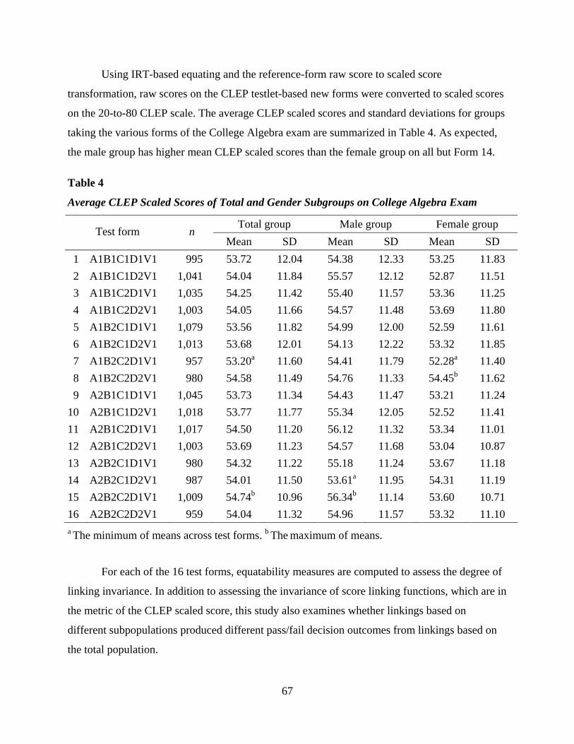
Using IRT-based equating and the reference-form raw score to scaled score

transformation, raw scores on the CLEP testlet-based new forms were converted to scaled scores

on the 20-to-80 CLEP scale. The average CLEP scaled scores and standard deviations for groups

taking the various forms of the College Algebra exam are summarized in Table 4. As expected,

the male group has higher mean CLEP scaled scores than the female group on all but Form 14.

Table 4

Average CLEP Scaled Scores of Total and Gender Subgroups on College Algebra Exam

Total group Male group Female group Test form n

Mean SD Mean SD Mean SD 1 A1B1C1D1V1 995 53.72 12.04 54.38 12.33 53.25 11.83 2 A1B1C1D2V1 1,041 54.04 11.84 55.57 12.12 52.87 11.51 3 A1B1C2D1V1 1,035 54.25 11.42 55.40 11.57 53.36 11.25 4 A1B1C2D2V1 1,003 54.05 11.66 54.57 11.48 53.69 11.80 5 A1B2C1D1V1 1,079 53.56 11.82 54.99 12.00 52.59 11.61 6 A1B2C1D2V1 1,013 53.68 12.01 54.13 12.22 53.32 11.85 7 A1B2C2D1V1 957 53.20a 11.60 54.41 11.79 52.28a 11.40 8 A1B2C2D2V1 980 54.58 11.49 54.76 11.33 54.45b 11.62 9 A2B1C1D1V1 1,045 53.73 11.34 54.43 11.47 53.21 11.24 10 A2B1C1D2V1 1,018 53.77 11.77 55.34 12.05 52.52 11.41 11 A2B1C2D1V1 1,017 54.50 11.20 56.12 11.32 53.34 11.01 12 A2B1C2D2V1 1,003 53.69 11.23 54.57 11.68 53.04 10.87 13 A2B2C1D1V1 980 54.32 11.22 55.18 11.24 53.67 11.18 14 A2B2C1D2V1 987 54.01 11.50 53.61a 11.95 54.31 11.19 15 A2B2C2D1V1 1,009 54.74b 10.96 56.34b 11.14 53.60 10.71 16 A2B2C2D2V1 959 54.04 11.32 54.96 11.57 53.32 11.10 a The minimum of means across test forms. b The maximum of means.

For each of the 16 test forms, equatability measures are computed to assess the degree of

linking invariance. In addition to assessing the invariance of score linking functions, which are in

the metric of the CLEP scaled score, this study also examines whether linkings based on

different subpopulations produced different pass/fail decision outcomes from linkings based on

the total population.

67

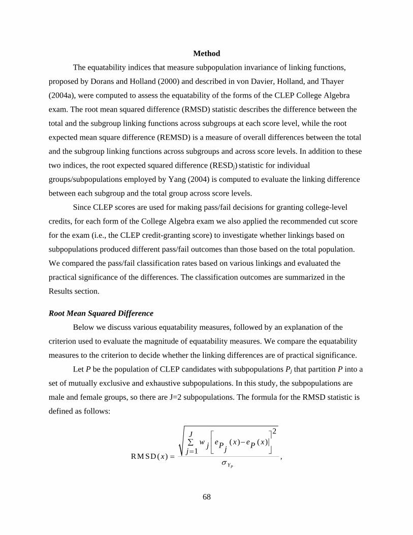
Method

The equatability indices that measure subpopulation invariance of linking functions,

proposed by Dorans and Holland (2000) and described in von Davier, Holland, and Thayer

(2004a), were computed to assess the equatability of the forms of the CLEP College Algebra

exam. The root mean squared difference (RMSD) statistic describes the difference between the

total and the subgroup linking functions across subgroups at each score level, while the root

expected mean square difference (REMSD) is a measure of overall differences between the total

and the subgroup linking functions across subgroups and across score levels. In addition to these

two indices, the root expected squared difference (RESDj) statistic for individual

groups/subpopulations employed by Yang (2004) is computed to evaluate the linking difference

between each subgroup and the total group across score levels.

Since CLEP scores are used for making pass/fail decisions for granting college-level

credits, for each form of the College Algebra exam we also applied the recommended cut score

for the exam (i.e., the CLEP credit-granting score) to investigate whether linkings based on

subpopulations produced different pass/fail outcomes than those based on the total population.

We compared the pass/fail classification rates based on various linkings and evaluated the

practical significance of the differences. The classification outcomes are summarized in the

Results section.

Root Mean Squared Difference

Below we discuss various equatability measures, followed by an explanation of the

criterion used to evaluate the magnitude of equatability measures. We compare the equatability

measures to the criterion to decide whether the linking differences are of practical significance.

Let P be the population of CLEP candidates with subpopulations Pj that partition P into a

set of mutually exclusive and exhaustive subpopulations. In this study, the subpopulations are

male and female groups, so there are J=2 subpopulations. The formula for the RMSD statistic is

defined as follows:

2( ) ( )

1RM SD ( ) ,

PY

Jw e x e xj P Pjj

xσ

⎡ ⎤−∑ ⎢ ⎥

⎣ ⎦==

68

where x is a raw score level on the testlet-based CLEP exam, denotes the function that

places x on the CLEP scale for the total population P, denotes the function that places x on

the CLEP scale for the subpopulation Pj,, wj is the proportion of Pj in P, and Σwj=1. The

denominator,

( )Pe x

( )jPe x

PYσ , is the standard deviation of the CLEP scaled score in the total population P

(Dorans & Holland, 2000).

Root Expected Squared Difference

The RESDj statistic is a weighted average of differences between a subpopulation linking

function and the total group linking function (Yang, 2004). The formula of the RESDj is defined

as below:

{ } { }22 ( ) ( )

( ) ( )0RESD = = ,

P Pp jP Pj

P P

Ze x e xxe x e xP x

jY Y

wE

σ σ

⎡ ⎤−⎢ ⎥⎡ ⎤ ⎣ ⎦−⎢ ⎥⎣ ⎦ =∑

where j denotes a subpopulation, EP{ }denotes averaging over raw score levels weighted by the

relative number of candidates at each score level in the total population P, Z is the maximum

possible raw score, wxP is xnn

in the total population P, and ΣwxP=1. Note that xn is the number of

candidates at raw score level of x, and is the total number of candidates. n

To compute RESDj at each score level, square the difference between the subpopulation

linking function and the total group linking function. Then, average these squared differences

across score levels weighted by the relative number of candidates in the total population at each

score level. Taking the square root of that weighted average and dividing the result by the

standard deviation of the composite score in the total population gives us a measure of RESDj in

the metric of the standard deviation of the CLEP scaled score.

Root Expected Mean Square Difference

REMSD is used to summarize linking differences across score levels and subpopulations.

Its formula is as follows:

69

2( ) ( )

1R EM SD = .

PY

Jw E e x e xj P P Pjj

σ

⎧ ⎫⎡ ⎤⎪ ⎪−∑ ⎨⎢ ⎥ ⎬⎪ ⎣ ⎦= ⎩ ⎭⎪

To be more expressive, we can rewrite the formula for REMSD as follows:

2 2

1 0 0 1

( ) ( ) ( ) ( )

REMSD or .P j P j

P P

J Z Z J

j x P P x j P Pj x x j

Y Y

w w e x e x w w e x e x

σ σ= = = =

⎡ ⎤ ⎡ ⎤− −⎣ ⎦ ⎣ ⎦=∑ ∑ ∑ ∑

REMSD is a double-weighted average of differences between subpopulation linking

functions and the total group linking function. At each score level, the difference between each

subpopulation linking function and the total group linking function is squared. These squared

differences are then averaged over subpopulations weighted by the relative size of each

subpopulation. Then these weighted sums of squared differences are averaged across score levels

weighted by the relative number of candidates in the total population at each score level. Taking

the square root of that weighted average and dividing the result by the standard deviation of the

composite score in the total population gives us a measure of overall equatability in the metric of

the standard deviation of the composite score (Dorans & Holland, 2000).

Hypothetical Total Group

If all the candidates had taken the same test form instead of the 16 different forms of the

CLEP College Algebra exam, the size of the total group for the form would be 16,121, which is

the sum of the observed sample sizes across the 16 forms (see Table 2). By using such a

hypothetical total group for each of the forms, we can work around potential problems due to

sampling variability, especially when observed sample sizes are small, for computing

equatability indices.

We estimated the frequency distribution of the hypothetical total group via the probability

density function for the theta (ability) estimate, produced by IRT-based equating with the Rasch

model. A standard normal distribution with a mean of 0 and standard deviation of 1 was assumed

70

for the thetas of the hypothetical total group. The frequency estimation procedure for the

hypothetical total group is summarized in the appendix. In computing equatability indices, we

used the estimated frequencies and the proportions of gender groups in the hypothetical total

group as weights. The drawback of using a hypothetical group is that errors may occur in

estimating its frequency distribution, which may then affect the equitability outcomes.

In addition to using the hypothetical total group data to control for sampling errors in

computing equatability indices, we also computed equatability indices using the data from each

of the observed total groups. By contrasting the two sets of outcomes for each form, we can

evaluate the appropriateness of the hypothetical and observed total group data.

Difference That Matters With the CLEP Exams

As mentioned earlier, CLEP scores are used for making decisions about granting college-

level course credits. The pass/fail decision depends on how a CLEP candidate’s score compares

to the recommended cut-score. For CLEP candidates a change in the pass/fail decision is the

difference that matters (DTM). Therefore, while evaluating linking differences, we focus on

CLEP test score levels around the pass/fail cut-score and compare the pass/fail classification

outcomes resulting from various linkings.

On the CLEP 20-to-80 score scale, half a score unit at the pass/fail threshold is crucial

because it may result in a reverse decision on pass/fail status. Therefore, we quantify the DTM

for CLEP to be half a CLEP scaled score unit when that score is at the threshold. For

comparisons across various exam forms, we further express the DTM in the standard deviation

unit, such that it represents the standard-score equivalent of half a CLEP score. This standardized

DTM is called SDTM in this paper.

The SDTM in standard deviation unit is useful in evaluating subpopulation invariance of

functions that link number-right raw scores and the CLEP scaled scores. We can compare the

RMSD/REMSD statistics to the SDTM to determine whether the linking differences are

practically significant. The linking differences across subpopulations are considered negligible if

the differences represented by the RMSD/REMSD are less than the SDTM. The practice of

ignoring differences that are less than half a score reporting unit has been used for years in the

equating practices of major testing programs, such as SAT (Dorans & Feigenbaum, 1994).

71

Computationally, dividing 0.5 by the standard deviation of the CLEP scores in the total

population gives us the SDTM. Over the 16 forms of the College Algebra exam the estimated

standard deviation of the CLEP scores in the hypothetical total group ranges from 9.46 to 9.54.

Accordingly, the SDTM based on the hypothetical total group data ranges from 0.052 to 0.053.

This paper uses SDTM* to denote the SDTM based on the hypothetical total group data

throughout, which should be differentiated from the SDTM that is based on the observed total-

group data.

The SDTM based on the observed total group data can be obtained by dividing 0.5 by the

sample standard deviation of the observed total group, treating the sample standard deviation as

the standard deviation of the total population for each form. As shown in Table 4, the observed

standard deviation of the CLEP scores ranges from 10.96 to 12.04 over the 16 forms. Therefore,

the SDTM based on the observed total group data ranges from 0.042 to 0.046 for these 16 forms.

Results

Equatability outcomes based on the hypothetical total group for the 16 forms of the CLEP

College Algebra exam are presented in this section, followed by an evaluation of the impact of

linking variation on pass/fail classifications.

Equatability of the CLEP College Algebra Exam

The RMSD outcomes are presented in figures that consist of a pair of plots for each of

the 16 College Algebra exam forms. The RESDj and the REMSD results are shown in tables.

RMSD results. Figures 1-16 each contains two plots, labeled a and b, respectively, for an

exam form. The plot labeled a shows the RMSD outcomes at various raw score levels, and the

RMSD values are compared to the corresponding SDTM* denoted by the broken line. To

facilitate the interpretation of the RMSD outcomes, the plot labeled b depicts the linking

differences between the total group and each of the gender subgroups.

72

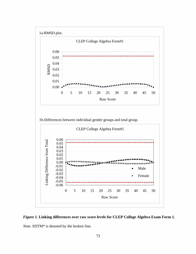
1a-RMSD plot.

1b-Differences between individual gender groups and total group.

CLEP College Algebra Form#1

0.000.010.020.030.040.050.06

0 5 10 15 20 25 30 35 40 45 50

Raw Score

RM

SD

CLEP College Algebra Form#1

-0.06-0.05-0.04-0.03-0.02-0.010.000.010.020.030.040.050.06

0 5 10 15 20 25 30 35 40 45 50

Raw Score

Link

ing

Diff

eren

ce fr

om T

otal

Male

Female

Figure 1. Linking differences over raw score levels for CLEP College Algebra Exam Form 1.

Note. SDTM* is denoted by the broken line.

73

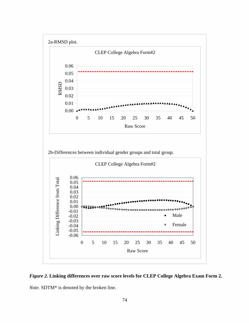
2a-RMSD plot.

2b-Differences between individual gender groups and total group.

CLEP College Algebra Form#2

0.000.010.020.030.040.050.06

0 5 10 15 20 25 30 35 40 45 50

Raw Score

RM

SD

CLEP College Algebra Form#2

-0.06-0.05-0.04-0.03-0.02-0.010.000.010.020.030.040.050.06

0 5 10 15 20 25 30 35 40 45 50

Raw Score

Link

ing

Diff

eren

ce fr

om T

otal

Male

Female

Figure 2. Linking differences over raw score levels for CLEP College Algebra Exam Form 2.

Note. SDTM* is denoted by the broken line.

74

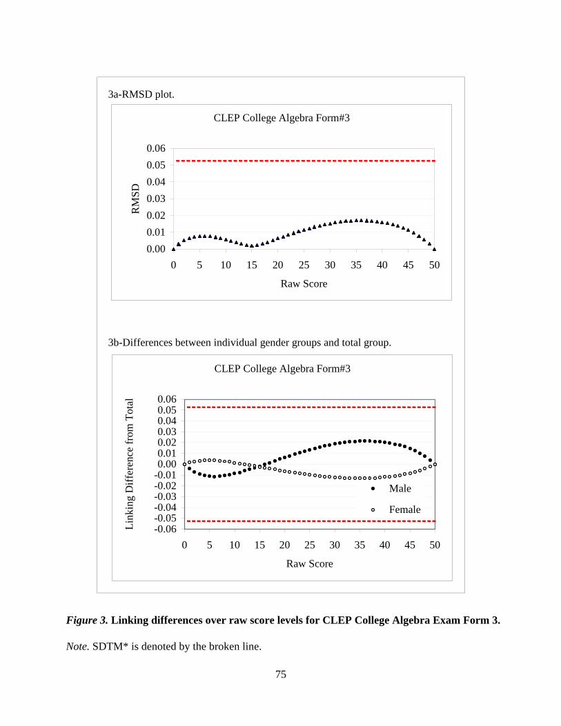
3a-RMSD plot.

3b-Differences between individual gender groups and total group.

CLEP College Algebra Form#3

0.000.010.020.030.040.050.06

0 5 10 15 20 25 30 35 40 45 50

Raw Score

RM

SD

CLEP College Algebra Form#3

-0.06-0.05-0.04-0.03-0.02-0.010.000.010.020.030.040.050.06

0 5 10 15 20 25 30 35 40 45 50

Raw Score

Link

ing

Diff

eren

ce fr

om T

otal

Male

Female

Figure 3. Linking differences over raw score levels for CLEP College Algebra Exam Form 3.

Note. SDTM* is denoted by the broken line.

75

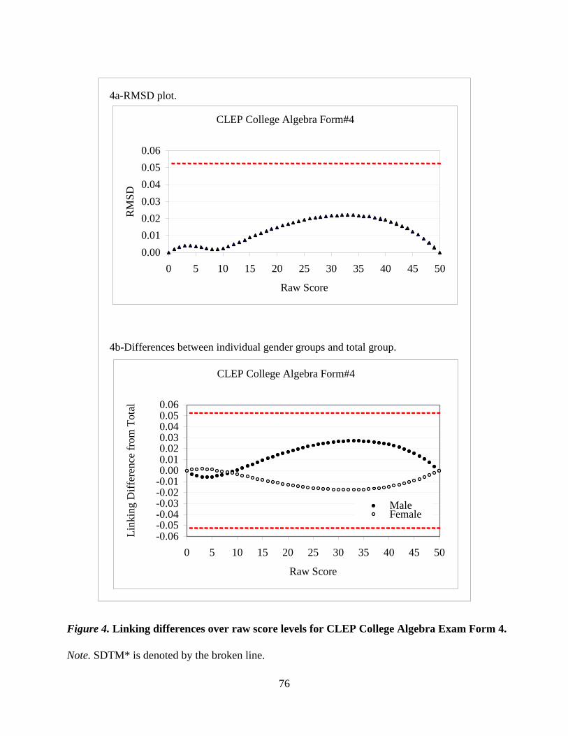
4a-RMSD plot.

4b-Differences between individual gender groups and total group.

CLEP College Algebra Form#4

0.000.010.020.030.040.050.06

0 5 10 15 20 25 30 35 40 45 50

Raw Score

RM

SD

CLEP College Algebra Form#4

-0.06-0.05-0.04-0.03-0.02-0.010.000.010.020.030.040.050.06

0 5 10 15 20 25 30 35 40 45 50

Raw Score

Link

ing

Diff

eren

ce fr

om T

otal

MaleFemale

Figure 4. Linking differences over raw score levels for CLEP College Algebra Exam Form 4.

Note. SDTM* is denoted by the broken line.

76

5a-RMSD plot.

5b-Differences between individual gender groups and total group.

CLEP College Algebra Form#5

0.000.010.020.030.040.050.06

0 5 10 15 20 25 30 35 40 45 50

Raw Score

RM

SD

CLEP College Algebra Form#5

-0.06-0.05-0.04-0.03-0.02-0.010.000.010.020.030.040.050.06

0 5 10 15 20 25 30 35 40 45 50

Raw Score

Link

ing

Diff

eren

ce fr

om T

otal

Male

Female

Figure 5. Linking differences over raw score levels for CLEP College Algebra Exam Form 5.

Note. SDTM* is denoted by the broken line.

77

6a-RMSD plot.

6b-Differences between individual gender groups and total group.

CLEP College Algebra Form#6

0.000.010.020.030.040.050.06

0 5 10 15 20 25 30 35 40 45 50

Raw Score

RM

SD

CLEP College Algebra Form#6

-0.06-0.05-0.04-0.03-0.02-0.010.000.010.020.030.040.050.06

0 5 10 15 20 25 30 35 40 45 50

Raw Score

Link

ing

Diff

eren

ce fr

om T

otal

Male

Female

Figure 6. Linking differences over raw score levels for CLEP College Algebra Exam Form 6.

Note. SDTM* is denoted by the broken line.

78

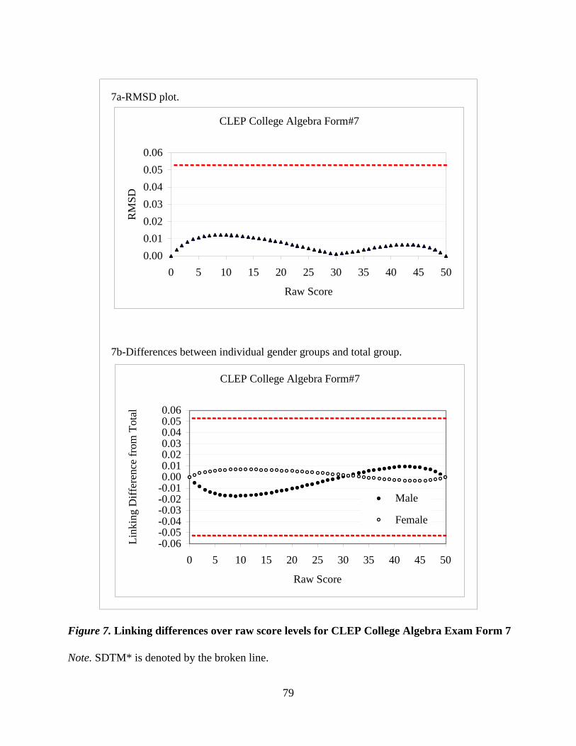
7a-RMSD plot.

7b-Differences between individual gender groups and total group.

CLEP College Algebra Form#7

0.000.010.020.030.040.050.06

0 5 10 15 20 25 30 35 40 45 50

Raw Score

RM

SD

CLEP College Algebra Form#7

-0.06-0.05-0.04-0.03-0.02-0.010.000.010.020.030.040.050.06

0 5 10 15 20 25 30 35 40 45 50

Raw Score

Link

ing

Diff

eren

ce fr

om T

otal

Male

Female

Figure 7. Linking differences over raw score levels for CLEP College Algebra Exam Form 7

Note. SDTM* is denoted by the broken line.

79

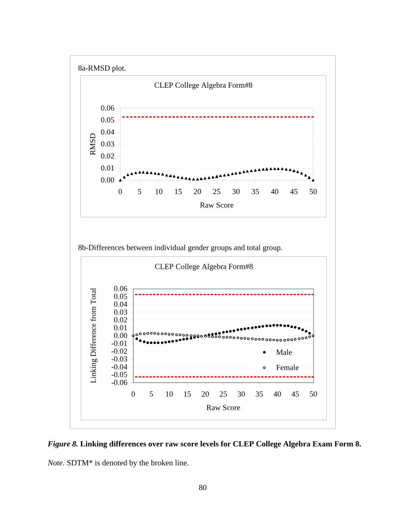
8a-RMSD plot.

8b-Differences between individual gender groups and total group.

CLEP College Algebra Form#8

0.000.010.020.030.040.050.06

0 5 10 15 20 25 30 35 40 45 50

Raw Score

RM

SD

CLEP College Algebra Form#8

-0.06-0.05-0.04-0.03-0.02-0.010.000.010.020.030.040.050.06

0 5 10 15 20 25 30 35 40 45 50

Raw Score

Link

ing

Diff

eren

ce fr

om T

otal

Male

Female

Figure 8. Linking differences over raw score levels for CLEP College Algebra Exam Form 8.

Note. SDTM* is denoted by the broken line.

80

9a-RMSD plot.

9b-Differences between individual gender groups and total group.

CLEP College Algebra Form#9

0.000.010.020.030.040.050.06

0 5 10 15 20 25 30 35 40 45 50

Raw Score

RM

SD

CLEP College Algebra Form#9

-0.06-0.05-0.04-0.03-0.02-0.010.000.010.020.030.040.050.06

0 5 10 15 20 25 30 35 40 45 50

Raw Score

Link

ing

Diff

eren

ce fr

om T

otal

Male

Female

Figure 9. Linking differences over raw score levels for CLEP College Algebra Exam Form 9.

Note. SDTM* is denoted by the broken line.

81

10a-RMSD plot.

10b-Differences between individual gender groups and total group.

CLEP College Algebra Form#10

0.000.010.020.030.040.050.06

0 5 10 15 20 25 30 35 40 45 50

Raw Score

RM

SD

CLEP College Algebra Form#10

-0.06-0.05-0.04-0.03-0.02-0.010.000.010.020.030.040.050.06

0 5 10 15 20 25 30 35 40 45 50

Raw Score

Link

ing

Diff

eren

ce fr

om T

otal

Male

Female

Figure 10. Linking differences over raw score levels for CLEP College Algebra Exam Form 10.

Note. SDTM* is denoted by the broken line.

82

11a-RMSD plot.

11b-Differences between individual gender groups and total group.

CLEP College Algebra Form#11

0.000.010.020.030.040.050.06

0 5 10 15 20 25 30 35 40 45 50

Raw Score

RM

SD

CLEP College Algebra Form#11

-0.06-0.05-0.04-0.03-0.02-0.010.000.010.020.030.040.050.06

0 5 10 15 20 25 30 35 40 45 50

Raw Score

Link

ing

Diff

eren

ce fr

om T

otal

Male

Female

Figure 11. Linking differences over raw score levels for CLEP College Algebra Exam Form 11.

Note. SDTM* is denoted by the broken line.

83

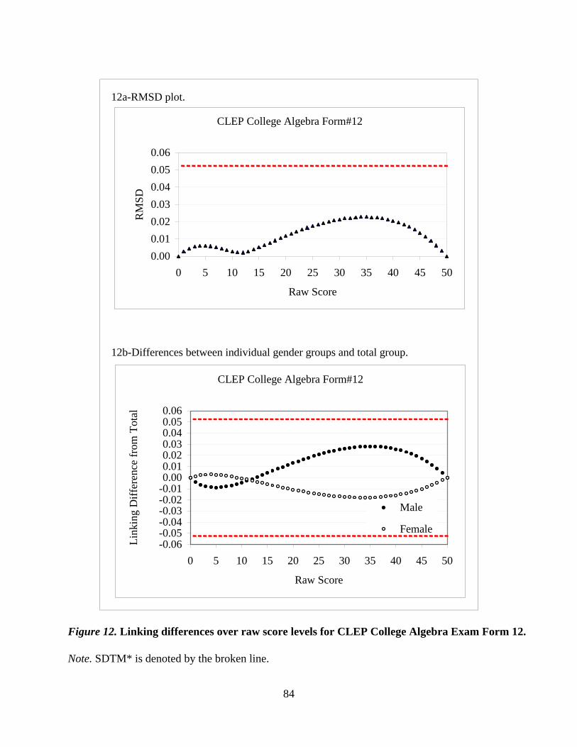
12a-RMSD plot.

12b-Differences between individual gender groups and total group.

CLEP College Algebra Form#12

0.000.010.020.030.040.050.06

0 5 10 15 20 25 30 35 40 45 50

Raw Score

RM

SD

CLEP College Algebra Form#12

-0.06-0.05-0.04-0.03-0.02-0.010.000.010.020.030.040.050.06

0 5 10 15 20 25 30 35 40 45 50

Raw Score

Link

ing

Diff

eren

ce fr

om T

otal

Male

Female

Figure 12. Linking differences over raw score levels for CLEP College Algebra Exam Form 12.

Note. SDTM* is denoted by the broken line.

84

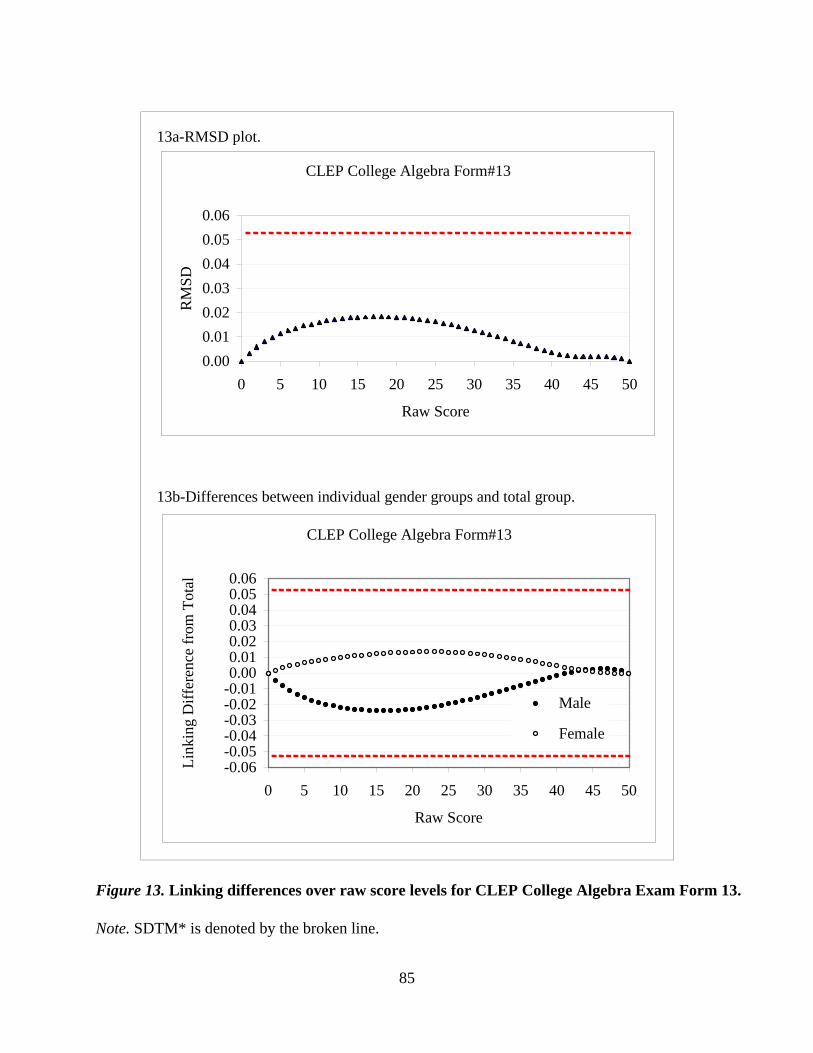
13a-RMSD plot.

13b-Differences between individual gender groups and total group.

CLEP College Algebra Form#13

0.000.010.020.030.040.050.06

0 5 10 15 20 25 30 35 40 45 50

Raw Score

RM

SD

CLEP College Algebra Form#13

-0.06-0.05-0.04-0.03-0.02-0.010.000.010.020.030.040.050.06

0 5 10 15 20 25 30 35 40 45 50

Raw Score

Link

ing

Diff

eren

ce fr

om T

otal

Male

Female

Figure 13. Linking differences over raw score levels for CLEP College Algebra Exam Form 13.

Note. SDTM* is denoted by the broken line.

85

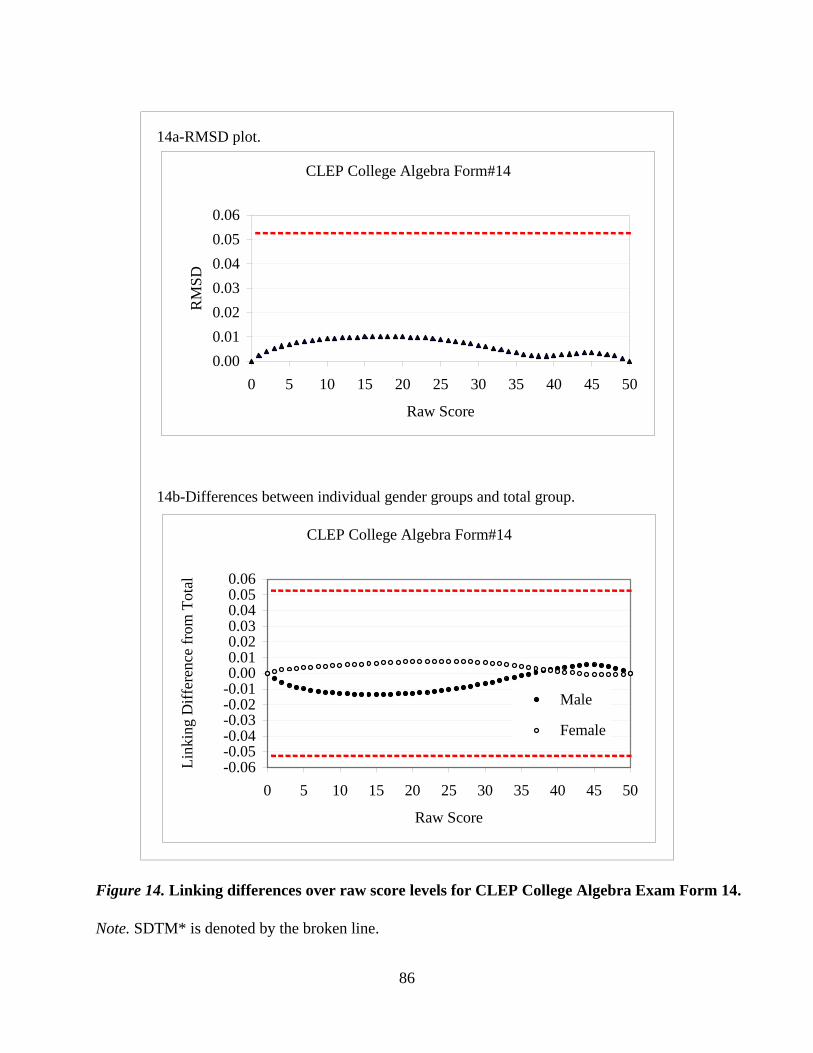
14a-RMSD plot.

14b-Differences between individual gender groups and total group.

CLEP College Algebra Form#14

0.000.010.020.030.040.050.06

0 5 10 15 20 25 30 35 40 45 50

Raw Score

RM

SD

CLEP College Algebra Form#14

-0.06-0.05-0.04-0.03-0.02-0.010.000.010.020.030.040.050.06

0 5 10 15 20 25 30 35 40 45 50

Raw Score

Link

ing

Diff

eren

ce fr

om T

otal

Male

Female

Figure 14. Linking differences over raw score levels for CLEP College Algebra Exam Form 14.

Note. SDTM* is denoted by the broken line.

86

15a-RMSD plot.

15b-Differences between individual gender groups and total group.

CLEP College Algebra Form#15

0.000.010.020.030.040.050.06

0 5 10 15 20 25 30 35 40 45 50

Raw Score

RM

SD

CLEP College Algebra Form#15

-0.06-0.05-0.04-0.03-0.02-0.010.000.010.020.030.040.050.06

0 5 10 15 20 25 30 35 40 45 50

Raw Score

Link

ing

Diff

eren

ce fr

om T

otal

Male

Female

Figure 15. Linking differences over raw score levels for CLEP College Algebra Exam Form 15.

Note. SDTM* is denoted by the broken line.

87

16a-RMSD plot.

16b-Differences between individual gender groups and total group.

CLEP College Algebra Form#16

0.000.010.020.030.040.050.06

0 5 10 15 20 25 30 35 40 45 50

Raw Score

RM

SD

CLEP College Algebra Form#16

-0.06-0.05-0.04-0.03-0.02-0.010.000.010.020.030.040.050.06

0 5 10 15 20 25 30 35 40 45 50

Raw Score

Link

ing

Diff

eren

ce fr

om T

otal

Male

Female

Figure 16. Linking differences over raw score levels for CLEP College Algebra Exam Form 16.

Note. SDTM* is denoted by the broken line.

88

Since the statistics in Figures 1-16 (for both plots labeled a and b) are based on the

hypothetical total group data, they should be compared to the SDTM* for practical significance.

These statistics have the same unit as the SDTM*, which is in the metric of the standard

deviation of the CLEP scores in the total population. By definition, the RMSD measures in the

plots labeled a are in the same metric. For the plots labeled b, the linking differences between

each gender group and the total group were transformed to have the same unit as the SDTM* to

facilitate comparisons.

The RMSD plots in Figures 1-16 show that across forms over raw score levels, none of

the RMSD measures is larger than 0.025. All of the RMSD values are much smaller than the

SDTM*, which ranges from 0.052 to 0.053. This suggests that the linking differences at various

score levels are negligible.

We further examined the plots labeled b in Figures 1-16, which show the magnitude and

direction of differences between the linking for a gender group and the linking for the total group

over raw score levels. Overall, the plots labeled b indicate that the linking for the female group is

more similar to the linking for the total group than the linking for the male group. In the plots,

the lines for the female group are closer to the zero lines for the total group. This is mainly

because there are more females than males in the total group. Nevertheless, neither the linking

for the female group nor the linking for the male group deviates from the linking for the total

group by more than 0.03 units at various raw score levels. That is, these linking differences are

smaller than the SDTM*. They are thus negligible.

REMSD and RESDj results. Table 5 shows the REMSD and the RESDj statistics for the

16 forms, respectively. As with the RMSD statistics presented earlier, the statistics in Table 5 are

based on the hypothetical total group. Over the 16 forms, the REMSD ranges from 0.0038 to

0.0177, well below the SDTM*, which ranges from 0.052 to 0.053. This suggests that the

linkings between the number-right raw scores and the CLEP scaled scores are invariant over

gender subpopulations for the CLEP College Algebra exam. The linking differences between the

total and gender groups are negligible.

89

Table 5

Equatability of the Multiple Forms of CLEP College Algebra Exam

Equatability index RESDj for individual subgroup Test form

Male Female REMSD

1 A1B1C1D1V1 0.0052 0.0021 0.0038 2 A1B1C1D2V1 0.0102 0.0066 0.0084 3 A1B1C2D1V1 0.0145 0.0096 0.0120 4 A1B1C2D2V1 0.0213 0.0144 0.0177 5 A1B2C1D1V1 0.0154 0.0105 0.0128 6 A1B2C1D2V1 0.0070 0.0055 0.0062 7 A1B2C2D1V1 0.0091 0.0042 0.0067 8 A1B2C2D2V1 0.0071 0.0028 0.0051 9 A2B1C1D1V1 0.0073 0.0028 0.0052 10 A2B1C1D2V1 0.0093 0.0059 0.0076 11 A2B1C2D1V1 0.0145 0.0093 0.0118 12 A2B1C2D2V1 0.0202 0.0137 0.0168 13 A2B2C1D1V1 0.0181 0.0116 0.0147 14 A2B2C1D2V1 0.0099 0.0065 0.0082 15 A2B2C2D1V1 0.0121 0.0058 0.0091 16 A2B2C2D2V1 0.0084 0.0034 0.0061

Note. The equatability indices are computed using estimated frequencies for a hypothetical total

group as weights. The hypothetical total group encompasses all candidates taking various alternate

forms (N = 16,121). Its frequency distribution is estimated based on the theta estimate, which is

resulted from IRT-based equating and has a standard normal distribution. In addition, the expected

proportional weights are used for the two gender groups in computing the equatability indices.

Specifically, the weight is 0.428 for the male group and 0.572 for the female group.

We further examine the RESDj outcomes for the gender subpopulations in Table 5. As

expected, the very small RESDj for both the male and female groups suggests a negligible

linking difference between each subgroup and the total group. The linking in the female group is

a bit more similar to that in the total group than the male group is since the female group

90

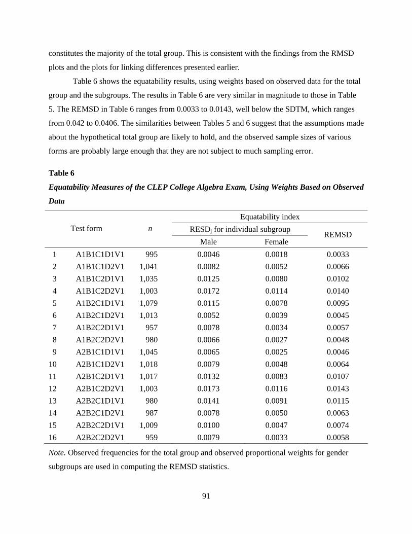
constitutes the majority of the total group. This is consistent with the findings from the RMSD

plots and the plots for linking differences presented earlier.

Table 6 shows the equatability results, using weights based on observed data for the total

group and the subgroups. The results in Table 6 are very similar in magnitude to those in Table

5. The REMSD in Table 6 ranges from 0.0033 to 0.0143, well below the SDTM, which ranges

from 0.042 to 0.0406. The similarities between Tables 5 and 6 suggest that the assumptions made

about the hypothetical total group are likely to hold, and the observed sample sizes of various

forms are probably large enough that they are not subject to much sampling error.

Table 6

Equatability Measures of the CLEP College Algebra Exam, Using Weights Based on Observed

Data

Equatability index RESDj for individual subgroup Test form n

Male Female REMSD

1 A1B1C1D1V1 995 0.0046 0.0018 0.0033 2 A1B1C1D2V1 1,041 0.0082 0.0052 0.0066 3 A1B1C2D1V1 1,035 0.0125 0.0080 0.0102 4 A1B1C2D2V1 1,003 0.0172 0.0114 0.0140 5 A1B2C1D1V1 1,079 0.0115 0.0078 0.0095 6 A1B2C1D2V1 1,013 0.0052 0.0039 0.0045 7 A1B2C2D1V1 957 0.0078 0.0034 0.0057 8 A1B2C2D2V1 980 0.0066 0.0027 0.0048 9 A2B1C1D1V1 1,045 0.0065 0.0025 0.0046 10 A2B1C1D2V1 1,018 0.0079 0.0048 0.0064 11 A2B1C2D1V1 1,017 0.0132 0.0083 0.0107 12 A2B1C2D2V1 1,003 0.0173 0.0116 0.0143 13 A2B2C1D1V1 980 0.0141 0.0091 0.0115 14 A2B2C1D2V1 987 0.0078 0.0050 0.0063 15 A2B2C2D1V1 1,009 0.0100 0.0047 0.0074 16 A2B2C2D2V1 959 0.0079 0.0033 0.0058

Note. Observed frequencies for the total group and observed proportional weights for gender

subgroups are used in computing the REMSD statistics.

91

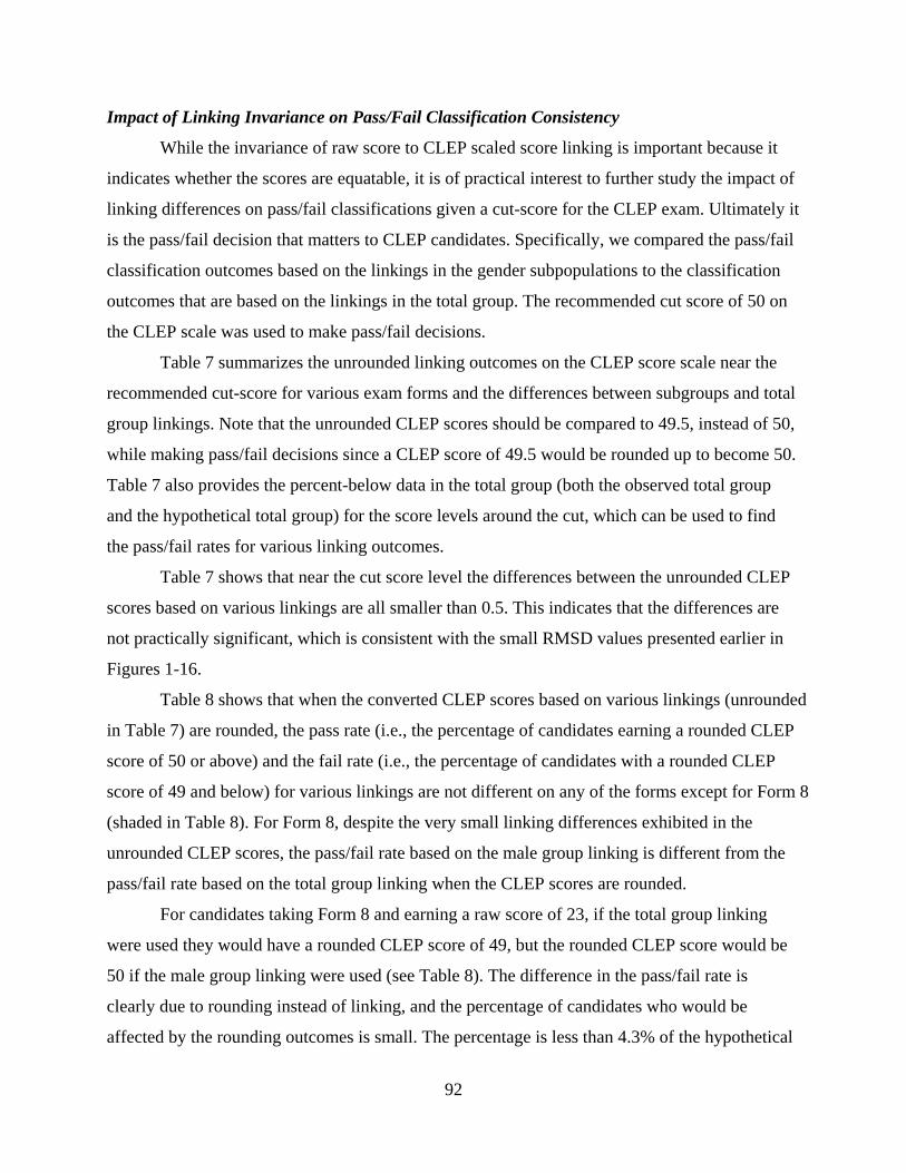
Impact of Linking Invariance on Pass/Fail Classification Consistency

While the invariance of raw score to CLEP scaled score linking is important because it

indicates whether the scores are equatable, it is of practical interest to further study the impact of

linking differences on pass/fail classifications given a cut-score for the CLEP exam. Ultimately it

is the pass/fail decision that matters to CLEP candidates. Specifically, we compared the pass/fail

classification outcomes based on the linkings in the gender subpopulations to the classification

outcomes that are based on the linkings in the total group. The recommended cut score of 50 on

the CLEP scale was used to make pass/fail decisions.

Table 7 summarizes the unrounded linking outcomes on the CLEP score scale near the

recommended cut-score for various exam forms and the differences between subgroups and total

group linkings. Note that the unrounded CLEP scores should be compared to 49.5, instead of 50,

while making pass/fail decisions since a CLEP score of 49.5 would be rounded up to become 50.

Table 7 also provides the percent-below data in the total group (both the observed total group

and the hypothetical total group) for the score levels around the cut, which can be used to find

the pass/fail rates for various linking outcomes.

Table 7 shows that near the cut score level the differences between the unrounded CLEP

scores based on various linkings are all smaller than 0.5. This indicates that the differences are

not practically significant, which is consistent with the small RMSD values presented earlier in

Figures 1-16.

Table 8 shows that when the converted CLEP scores based on various linkings (unrounded

in Table 7) are rounded, the pass rate (i.e., the percentage of candidates earning a rounded CLEP

score of 50 or above) and the fail rate (i.e., the percentage of candidates with a rounded CLEP

score of 49 and below) for various linkings are not different on any of the forms except for Form 8

(shaded in Table 8). For Form 8, despite the very small linking differences exhibited in the

unrounded CLEP scores, the pass/fail rate based on the male group linking is different from the

pass/fail rate based on the total group linking when the CLEP scores are rounded.

For candidates taking Form 8 and earning a raw score of 23, if the total group linking

were used they would have a rounded CLEP score of 49, but the rounded CLEP score would be

50 if the male group linking were used (see Table 8). The difference in the pass/fail rate is

clearly due to rounding instead of linking, and the percentage of candidates who would be

affected by the rounding outcomes is small. The percentage is less than 4.3% of the hypothetical

92

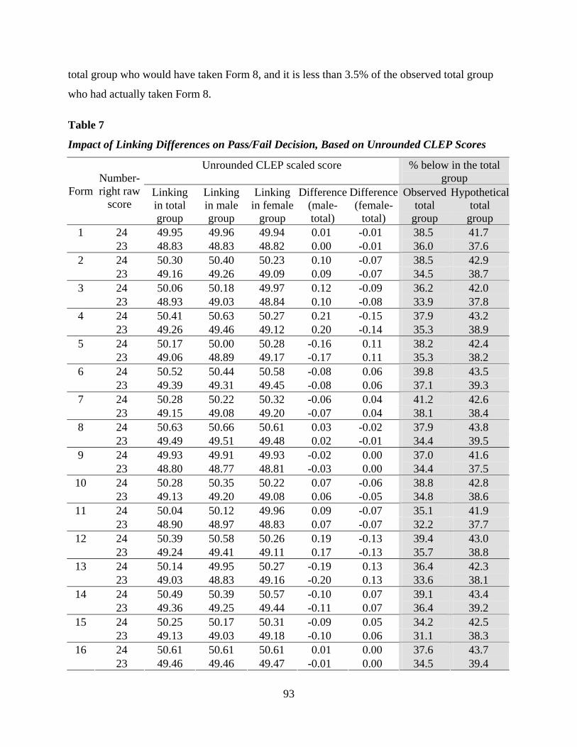
total group who would have taken Form 8, and it is less than 3.5% of the observed total group

who had actually taken Form 8.

Table 7

Impact of Linking Differences on Pass/Fail Decision, Based on Unrounded CLEP Scores

Unrounded CLEP scaled score % below in the total group

Form Number-right raw

score Linking in total group

Linking in male group

Linking in female

group

Difference (male-total)

Difference (female-

total)

Observed total

group

Hypothetical total

group 24 49.95 49.96 49.94 0.01 -0.01 38.5 41.7 1 23 48.83 48.83 48.82 0.00 -0.01 36.0 37.6 24 50.30 50.40 50.23 0.10 -0.07 38.5 42.9 2 23 49.16 49.26 49.09 0.09 -0.07 34.5 38.7 24 50.06 50.18 49.97 0.12 -0.09 36.2 42.0 3 23 48.93 49.03 48.84 0.10 -0.08 33.9 37.8 24 50.41 50.63 50.27 0.21 -0.15 37.9 43.2 4 23 49.26 49.46 49.12 0.20 -0.14 35.3 38.9 24 50.17 50.00 50.28 -0.16 0.11 38.2 42.4 5 23 49.06 48.89 49.17 -0.17 0.11 35.3 38.2 24 50.52 50.44 50.58 -0.08 0.06 39.8 43.5 6 23 49.39 49.31 49.45 -0.08 0.06 37.1 39.3 24 50.28 50.22 50.32 -0.06 0.04 41.2 42.6 7 23 49.15 49.08 49.20 -0.07 0.04 38.1 38.4 24 50.63 50.66 50.61 0.03 -0.02 37.9 43.8 8 23 49.49 49.51 49.48 0.02 -0.01 34.4 39.5 24 49.93 49.91 49.93 -0.02 0.00 37.0 41.6 9 23 48.80 48.77 48.81 -0.03 0.00 34.4 37.5 24 50.28 50.35 50.22 0.07 -0.06 38.8 42.8 10 23 49.13 49.20 49.08 0.06 -0.05 34.8 38.6 24 50.04 50.12 49.96 0.09 -0.07 35.1 41.9 11 23 48.90 48.97 48.83 0.07 -0.07 32.2 37.7 24 50.39 50.58 50.26 0.19 -0.13 39.4 43.0 12 23 49.24 49.41 49.11 0.17 -0.13 35.7 38.8 24 50.14 49.95 50.27 -0.19 0.13 36.4 42.3 13 23 49.03 48.83 49.16 -0.20 0.13 33.6 38.1 24 50.49 50.39 50.57 -0.10 0.07 39.1 43.4 14 23 49.36 49.25 49.44 -0.11 0.07 36.4 39.2 24 50.25 50.17 50.31 -0.09 0.05 34.2 42.5 15 23 49.13 49.03 49.18 -0.10 0.06 31.1 38.3 24 50.61 50.61 50.61 0.01 0.00 37.6 43.7 16 23 49.46 49.46 49.47 -0.01 0.00 34.5 39.4

93

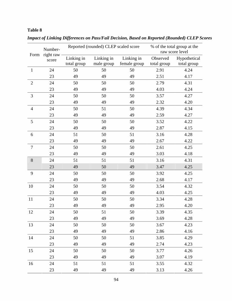
Table 8

Impact of Linking Differences on Pass/Fail Decision, Based on Reported (Rounded) CLEP Scores

Reported (rounded) CLEP scaled score % of the total group at the raw score level Form

Number-right raw

score Linking in total group

Linking in male group

Linking in female group

Observed total group

Hypothetical total group

24 50 50 50 2.91 4.24 1 23 49 49 49 2.51 4.17 24 50 50 50 2.79 4.31 2 23 49 49 49 4.03 4.24 24 50 50 50 3.57 4.27 3 23 49 49 49 2.32 4.20 24 50 51 50 4.39 4.34 4 23 49 49 49 2.59 4.27 24 50 50 50 3.52 4.22 5 23 49 49 49 2.87 4.15 24 51 50 51 3.16 4.28 6 23 49 49 49 2.67 4.22 24 50 50 50 2.61 4.25 7 23 49 49 49 3.03 4.18 24 51 51 51 3.16 4.31 8 23 49 50 49 3.47 4.25 24 50 50 50 3.92 4.25 9 23 49 49 49 2.68 4.17 24 50 50 50 3.54 4.32 10 23 49 49 49 4.03 4.25 24 50 50 50 3.34 4.28 11 23 49 49 49 2.95 4.20 24 50 51 50 3.39 4.35 12 23 49 49 49 3.69 4.28 24 50 50 50 3.67 4.23 13 23 49 49 49 2.86 4.16 24 50 50 51 3.85 4.29 14 23 49 49 49 2.74 4.23 24 50 50 50 3.77 4.26 15 23 49 49 49 3.07 4.19 24 51 51 51 3.55 4.32 16 23 49 49 49 3.13 4.26

94

In general, the pass/fail rates that resulted from linkings in the gender subpopulations are

consistent with the outcomes that resulted from linkings in the total group. The only inconsistent

case (on Form 8) is attributed to rounding but not linking. It is therefore reasonable to conclude

that there is no impact of subpopulation linkings on the pass/fail classification for the CLEP

College Algebra exam.

Summary and Suggestion

This research demonstrates how population invariance checks could be applied to

evaluate linking outcomes involving IRT-based equating for testlet-based exams. Overall, the

linking outcomes are invariant over gender subpopulations for all of the 16 forms of the CLEP

College Algebra exam. The linking differences between the gender groups and the total group

are very small for all of the forms. Even for Form 14, for which the candidate group and/or the

test form look somewhat different from the rest, the equatability indices are small enough to

suggest negligible linking differences. Equatability outcomes based on the hypothetical and the

observed total groups are very similar, which provides evidence of the tenability of the

equatability measures in this study.

The CLEP exam studied in this research is not prone to multidimensionality problems

because of its content and the nature of the subject matter. Hence, the Rasch model can

appropriately be used for linking purposes. For other CLEP exams that are subject to

multidimensionality problems, linking outcomes may become problematic due to inadequate

equating/linking and/or failure in calibration using the Rasch model. In such cases, equatability

measures can still be used to detect possible linking differences and to evaluate the robustness of

the Rasch model. Although we may not be able to attribute significant linking difference, if there

is any, to problematic equating/linking or to the Rasch model, it is important to detect and

document such differences for operational enhancement. Also, if we find no significant linking

differences in such cases, the Rasch model is likely to be robust. Thus, in addition to the

invariant linking outcomes for the College Algebra exam presented in this study, we recommend

that other CLEP exams for different subject matters be studied to determine the adequacy of

linkings and scoring.

95

Notes

1 The American Council on Education (ACE) conducts periodic reviews of the CLEP program,

including the processes to determine the recommended credit-granting score. The ACE

recommends a credit-granting score of 50 for various CLEP exams, effective July 2001.

2 Although the common reference form used in this study differed from the testlet-based new

forms in test construction, length, and scoring method, this reference form was useful in

maintaining the credit-granting standard for the CLEP College Algebra exam before a new

standard could be established on the testlet-based form via standard setting. Since a standard-

setting study was conducted recently and since May 2005 all the testlet-based forms have been

equated to a new testlet-based reference form, the linking procedure described in this study is no

longer used operationally for the College Algebra exam.

96

Appendix

Procedure for Deriving the Frequency Distributions for the Hypothetical Total Groups

We assumed a standard normal distribution (with 0μ = and 1σ = ) for the ability (θ ) of

the hypothetical total group for each of the 16 forms of the CLEP College Algebra exam. Based

on the assumption, for each raw score level of an exam form, we used the standard normal

probability density function (2

21( ) ( )2

f eθ

θπ

−= ) to estimate the probability density in the

hypothetical total group for the ability estimate (θ ) resulted from the IRT-based equating with

the Rasch model. Based on the resulting probability density estimates, we then calculated the

relative frequencies for different raw score levels for the hypothetical total group. This

estimation procedure was applied to all the 16 forms of the CLEP exam. See Table A1 for an

example of such estimation outcomes.

Table A1

Example Outcomes of Estimating Frequencies at Various Raw Score Levels for the

Hypothetical Total Group on a CLEP College Algebra Exam Form

Raw score

Theta estimate Standard normal probability density

Relative frequency

… … … … … … … … … … … … 30 0.418705 0.3655 0.0393 29 0.321705 0.3788 0.0408 28 0.225867 0.3889 0.0418 27 0.1309 0.3955 0.0426 26 0.036507 0.3987 0.0429 25 -0.05752 0.3983 0.0429 24 -0.151501 0.3944 0.0424 23 -0.24567 0.3871 0.0417 22 -0.340322 0.3765 0.0405 21 -0.435708 0.3628 0.0390 … … … … … … … … … … … …

97

Assuming that all the examinees took the same exam form instead of the 16 different

forms, the size of the hypothetical total group for each of the 16 forms would be 16,121, which is

the sum of the observed sample sizes across the 16 forms. By multiplying the estimated relative

frequencies for a form by 16,121, we obtained the frequency estimates for the hypothetical total

group for each of the 16 forms.

98

99

Invariance of Equating Functions Across Different Subgroups of Examinees

Taking a Science Achievement Test

Qing Yi

Harcourt Assessment, Inc., San Antonio, TX

Deborah J. Harris and Xiaohong Gao

ACT, Inc., Iowa City, IA

100

Abstract

This study investigates the group invariance of equating results using a science achievement test.

Examinees were divided into different subgroups based on the average composite score for test

centers, whether they had taken a physics course, and self-reported science GPA. Results

indicate that the conversions obtained from different subgroups were similar to the conversions

obtained by using the total group, except when the groups were divided based on whether a

student had taken a physics course. Where there were differences, the differences were generally

one equated raw score point.

Key words: Group invariance, score equating, equating conversions, IRT true score and observed

score equating methods

101

Acknowledgments

The authors are grateful to Dan Eignor and Anne Fitzpatrick for helpful comments on an earlier

version of the paper.

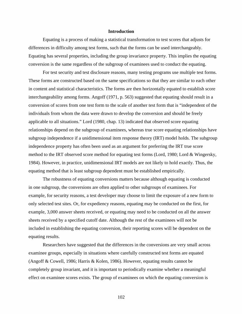
102

Introduction

Equating is a process of making a statistical transformation to test scores that adjusts for

differences in difficulty among test forms, such that the forms can be used interchangeably.

Equating has several properties, including the group invariance property. This implies the equating

conversion is the same regardless of the subgroup of examinees used to conduct the equating.

For test security and test disclosure reasons, many testing programs use multiple test forms.

These forms are constructed based on the same specifications so that they are similar to each other

in content and statistical characteristics. The forms are then horizontally equated to establish score

interchangeability among forms. Angoff (1971, p. 563) suggested that equating should result in a

conversion of scores from one test form to the scale of another test form that is “independent of the

individuals from whom the data were drawn to develop the conversion and should be freely

applicable to all situations.” Lord (1980, chap. 13) indicated that observed score equating

relationships depend on the subgroup of examinees, whereas true score equating relationships have

subgroup independence if a unidimensional item response theory (IRT) model holds. The subgroup

independence property has often been used as an argument for preferring the IRT true score

method to the IRT observed score method for equating test forms (Lord, 1980; Lord & Wingersky,

1984). However, in practice, unidimensional IRT models are not likely to hold exactly. Thus, the

equating method that is least subgroup dependent must be established empirically.

The robustness of equating conversions matters because although equating is conducted

in one subgroup, the conversions are often applied to other subgroups of examinees. For

example, for security reasons, a test developer may choose to limit the exposure of a new form to

only selected test sites. Or, for expediency reasons, equating may be conducted on the first, for

example, 3,000 answer sheets received, or equating may need to be conducted on all the answer

sheets received by a specified cutoff date. Although the rest of the examinees will not be

included in establishing the equating conversion, their reporting scores will be dependent on the

equating results.

Researchers have suggested that the differences in the conversions are very small across

examinee groups, especially in situations where carefully constructed test forms are equated

(Angoff & Cowell, 1986; Harris & Kolen, 1986). However, equating results cannot be

completely group invariant, and it is important to periodically examine whether a meaningful

effect on examinee scores exists. The group of examinees on which the equating conversion is

103

developed should be clearly defined. Dorans and Holland (2000) introduce general measures for

evaluating group invariance by comparing equating results obtained on subgroups with those

obtained on the total group of examinees.

Several studies have examined group invariance issues based on racial/ethnical

background, gender, geographic region, and other naturally occurring variables to obtain

subgroups (e.g., Dorans, Holland, Thayer, & Tateneni, 2002; Yang, Dorans, & Tateneni, 2002).

Relatively comparable equating results have been found when equating is conducted on the total

group and such subgroups, if test forms are constructed to be parallel in content and statistical

characteristics and if an appropriate data collection design is used for a particular equating method.

However, research (Cook & Petersen, 1987) also has shown that if subgroups are constructed

using variables that are related to the construct being measured, equating results then may be

different for the total group and the subgroups. The purpose of this paper was to continue this line

of research by dividing examinees into subgroups based on various measures of ability using a

science achievement test. See below for details on assigning examinees to different subgroups.

Methods

A science achievement test was used as a data source in this study; it was administered

primarily to juniors and seniors in high schools, as part of a battery of tests that included a

questionnaire relating to high school courses and grades. A composite score can be computed

based on the scale scores obtained from each of the tests in the battery.

Three forms (Forms A, B, and C) of the science test administered to randomly equivalent

groups of examinees in a single administration in one year were used in this study. Possible raw

scores range from 0 to 40 in increments of 1. Form A served as a base form, and the raw scores

on the other two forms (B and C) were equated to the raw scores on Form A, using IRT true and

observed score equating methods (Kolen & Brennan, 2004). Form B was also equated to Form A

using classical equipercentile equating method (Kolen & Brennan). These equating methods are

appropriate for the data collection design used to obtain the data for this study.

Cook and Petersen (1987) indicated that examinees who choose to take a test on a

particular administration date may have different characteristics than examinees who choose

another test date. One group of examinees may be more able, or they may have taken more

relevant courses. Thus, in this study, equatings were conducted using the total group, as well as

high and low ability groups, where ability was determined in different ways. First, another test

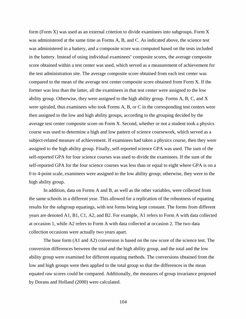
104

form (Form X) was used as an external criterion to divide examinees into subgroups. Form X

was administered at the same time as Forms A, B, and C. As indicated above, the science test

was administered in a battery, and a composite score was computed based on the tests included

in the battery. Instead of using individual examinees’ composite scores, the average composite

score obtained within a test center was used, which served as a measurement of achievement for

the test administration site. The average composite score obtained from each test center was

compared to the mean of the average test center composite score obtained from Form X. If the

former was less than the latter, all the examinees in that test center were assigned to the low

ability group. Otherwise, they were assigned to the high ability group. Forms A, B, C, and X

were spiraled, thus examinees who took Forms A, B, or C in the corresponding test centers were

then assigned to the low and high ability groups, according to the grouping decided by the

average test center composite score on Form X. Second, whether or not a student took a physics

course was used to determine a high and low pattern of science coursework, which served as a

subject-related measure of achievement. If examinees had taken a physics course, then they were

assigned to the high ability group. Finally, self-reported science GPA was used. The sum of the

self-reported GPA for four science courses was used to divide the examinees. If the sum of the

self-reported GPA for the four science courses was less than or equal to eight where GPA is on a

0 to 4-point scale, examinees were assigned to the low ability group; otherwise, they were in the

high ability group.

In addition, data on Forms A and B, as well as the other variables, were collected from

the same schools in a different year. This allowed for a replication of the robustness of equating

results for the subgroup equatings, with test forms being kept constant. The forms from different

years are denoted A1, B1, C1, A2, and B2. For example, A1 refers to Form A with data collected

at occasion 1, while A2 refers to Form A with data collected at occasion 2. The two data

collection occasions were actually two years apart.

The base form (A1 and A2) conversion is based on the raw score of the science test. The

conversion differences between the total and the high ability group, and the total and the low

ability group were examined for different equating methods. The conversions obtained from the

low and high groups were then applied to the total group so that the differences in the mean

equated raw scores could be compared. Additionally, the measures of group invariance proposed

by Dorans and Holland (2000) were calculated.

105

The three-parameter logistic IRT model was used to calibrate item parameters with the

BILOG-MG (Zimowski, Muraki, Mislevy, & Bock, 1996) computer program. The item

parameters were calibrated for each form on the total group and each subgroup, respectively. IRT

true and observed score equating methods and an equipercentile equating method (for details see

Kolen & Brennan, 2004) with cubic spline postsmoothing were used to equate the test forms.

Measures of Group Invariance

Dorans and Holland (2000) introduced an index called the root mean squared difference

(RMSD) to quantify group invariance of random group equating. The RMSD compares equating

results computed on different subgroups with the result computed for the total group. The

formula for the RMSD is

P

j

Y

jPPj xexew

xRMSDσ

∑ −=

2)]()([)( (1)

where x is a raw score point; P is the total group of examinees from which the subgroups were

divided; )(xeP denotes the equating function that equates X to Y on the total group of examinees

P; )(xejP denotes the equating function that equates X to Y on the subgroup jP of P; and jw

denotes the weight, which could be the relative proportion of jP in P or some other set of

weights that sum to unity. In this study, jw is the relative proportion of jP in P. The

denominatorPYσ is the standard deviation of Y in P. The set of subgroups partitions P into a set

of mutually exclusive and exhaustive subgroups.

In addition to RMSD(x) that provides a value for each score point of X, Dorans and

Holland (2000) also introduced a summary measure called the root expected mean squared

difference (REMSD) that is defined as

P

j

Y

jPPPj xexeEw

REMSDσ

∑ −=

})]()({[ 2

(2)

where x denotes a random score from the total group P, and EP{ } denotes averaging over the

distribution of X in P. REMSD is a weighted average of differences between the subgroup

equating function and the total group equating function.

106

Results

Raw score descriptive statistics on all the forms for the total group and each of the

subgroups are listed in Tables 1 through 5. Tables 6 and 7 present the percentages of examinees

and the equated raw scores based on different equating methods and grouping variables (i.e., test

center average composite score, whether the examinees had taken a physics course, and self-

reported science GPA) at each of the three specific raw score points (19, 23, and 25). Table 8

contains the REMSD for different equating methods on the subgroups. The magnitude of the

REMSD is decided based on difference that matters (DTM, see below). Figures 1 through 9

present the conversion differences between the total and high ability group and the total and low

ability group. Figures 10 through 12 show the equated raw score mean differences between

subgroups. Figures 13 through 15 display the RMSD across the raw score range for different

equating methods. The rounded equated raw score is used to summarize the results of this study

whenever appropriate.

Tables 1 to 5 indicate that the differences of the mean raw scores between the two

subgroups were small when the subgroups were obtained based on the average composite scores

for test centers (one raw score point or less). However, this difference became larger when the

subgroups were divided based on whether or not the student had taken a physics course (close to

five raw score points) or based on the sum of the self-reported science courses GPA (at least

three raw score points).

Table 1

Raw Score Descriptive Statistics of Form A1 for the Total, Composite Score, Course Taken,

and GPA Groups

Group N Mean SD Total 3,656 23.67 6.77 Composite low 1,662 23.09 6.84 Composite high 1,994 24.15 6.67 Course taken low 2,247 21.75 6.49 Course taken high 1,409 26.72 6.04 GPA low 2,242 22.14 6.69 GPA high 1,414 26.10 6.15

107

Table 2

Raw Score Descriptive Statistics of Form B1 for the Total, Composite Score, Course Taken,

and GPA Groups

Group N Mean SD Total 3,414 23.33 5.90 Composite low 1,552 22.80 5.86 Composite high 1,862 23.76 5.90 Course taken low 2,084 21.75 5.48 Course taken high 1,330 25.79 5.71 GPA low 2,009 21.85 5.76 GPA high 1,405 25.43 5.46

Table 3

Raw Score Descriptive Statistics of Form C1 for the Total, Composite Score, Course Taken,

and GPA Groups

Group N Mean SD Total 3,645 23.06 6.95 Composite low 1,661 22.30 7.08 Composite high 1,984 23.70 6.77 Course taken low 2,225 21.16 6.55 Course taken high 1,420 26.04 6.50 GPA low 2,167 21.22 6.84 GPA high 1,478 25.76 6.19

Table 4

Raw Score Descriptive Statistics of Form A2 for the Total, Composite Score, Course Taken,

and GPA Groups

Group N Mean SD Total 2,663 23.94 6.78 Composite low 1,166 23.31 6.68 Composite high 1,497 24.43 6.83 Course taken low 1,717 22.24 6.54 Course taken high 946 27.02 6.11 GPA low 1,507 22.10 6.64 GPA high 1,156 26.34 6.20

108

Table 5

Raw Score Descriptive Statistics of Form B2 for the Total, Composite Score, Course Taken,

and GPA Groups

Group N Mean SD Total 2,633 23.47 6.01 Composite low 1,150 22.99 6.05 Composite high 1,483 23.85 5.96 Course taken low 1,722 22.34 5.80 Course taken high 911 25.62 5.82 GPA low 1,484 22.14 5.91 GPA high 1,149 25.20 5.70

Comparison of Conversions Derived From Different Subgroups

Groups assigned according to test center average composite scores. The conversions for

Form B1 from both the high and low groups according to the test center average composite

scores were similar to the conversion from the total group at the middle part of the raw score

range, with only an occasional one equated raw score point difference (see Figure 1). In other

words, using different subgroups based on the test center average composite scores provided

similar equated raw score conversions for those receiving raw scores between 16 and 30. The

results were consistent across the IRT true and observed score equating methods and the classical

equipercentile equating methods. However, the conversions obtained from the high and low

groups differed from the conversion obtained from the total group by one equated raw score

point (either higher or lower) for many raw scores less than 16 or larger than 30. The differences

also occurred at the lower raw score range in Form C1 (Figure 2).

The conversions for Form B2 from both the high and low groups were more similar to the

conversion from the total group at raw scores above 19 than at raw scores below 19 (see Figure

3). The equipercentile equating resulted in more similar subgroup raw score conversions

compared to the total group conversion than the IRT equating methods. The differences were at

most one equated raw score point (either higher or lower).

Groups assigned according to whether or not examinees took a physics course. The

conversions for Form B1 from the high and low groups according to whether examinees took a

physics course were different from the conversion for the total group at many raw score points

109

(see Figure 4). At raw scores below 23, the equated raw scores from the high group were mostly

higher than the equated scores from the total group. The results were consistent across the IRT

true and observed score and the classical equipercentile equating methods. A similar pattern was

also found in Form C1 (Figure 5).

The conversions for Form B2 from the high group were also higher than the conversion

from the total group at most of the raw score points (see Figure 6). Most of the differences were

one equated raw score point, but some differed by two equated raw score points. The use of the

low group in equatings produced either the same or lower equated raw scores than the use of the

total group. This finding was consistent across different equating methods for Form B2.

Groups assigned according to self-reported science GPA. The conversion for Form B1

from the low GPA group was more similar to the conversion for the total group than the

conversion for the high GPA group was (see Figure 7). The use of the high GPA group appeared

to produce lower raw score conversions, and the use of the low GPA group appeared to produce

higher raw score conversions at some score points. A similar pattern was observed for Form C1

(Figure 8). This pattern is different from what was found when groups were divided as to

whether they had taken a physics course. All the differences between the total and the high or

low science GPA groups were within one equated raw score point (except for Form C1, where

there was a two-point difference in the IRT true score equating at a raw score of 9).

The conversions for Form B2 from the high group were higher than the conversion for

the total group at most of the raw score points (see Figure 9). Most of the differences were one

equated raw score point. The use of the low group in equatings produced either the same or

lower equated raw scores than the use of the total group. This finding is consistent across

different equating methods for Form B2, and it is also consistent with what was found when the

groups were divided based on whether the examinees had taken a physics course.

The raw score distribution for each of the forms indicates that there are more

observations in the middle of the score range and fewer examinees at the two ends. The sampling

errors at the two ends may result in the differences in the conversions observed in Figures 1 to 9.

The variability of item parameter estimates may affect the IRT equating results; however, the

stability of item parameter estimations is not the focus of this study.

110

Figure 1. Form B1 conversion differences between total and high groups and total and low

groups when groups were defined based on a third form overall average composite score.

IRT True Score Equating

-2.5-2.0-1.5-1.0-0.50.00.51.01.52.02.5

0 2 4 6 8 10 12 14 16 18 20 22 24 26 28 30 32 34 36 38 40

Raw Score

Con

vers

ion

Diff

eren

ceTotal-High Total-Low

IRT Observed Score Equating

-2.5-2.0-1.5-1.0-0.50.00.51.01.52.02.5

0 2 4 6 8 10 12 14 16 18 20 22 24 26 28 30 32 34 36 38 40

Raw Score

Con

vers

ion

Diff

eren

ce

Total-High Total-Low

Equipercentile Equating

-2.5-2.0-1.5-1.0-0.50.00.51.01.52.02.5

0 2 4 6 8 10 12 14 16 18 20 22 24 26 28 30 32 34 36 38 40

Raw Score

Con

vers

ion

Diff

eren

ce

Total-High Total-Low

111

Figure 2. Form C1 conversion differences between total and high groups and total and low

groups when groups were defined based on a third form overall average composite score.

IRT True Score Equating

-2.5

-2.0

-1.5

-1.0

-0.5

0.0

0.5

1.0

1.5

2.0

2.5

0 2 4 6 8 10 12 14 16 18 20 22 24 26 28 30 32 34 36 38 40

Raw Score

Con

vers

ion

Diff

eren

ceTotal-High Total-Low

IRT Observed Score Equating

-2.5

-2.0

-1.5

-1.0

-0.5

0.0

0.5

1.0

1.5

2.0

2.5

0 2 4 6 8 10 12 14 16 18 20 22 24 26 28 30 32 34 36 38 40

Raw Score

Con

vers

ion

Diff

eren

ce

Total-High Total-Low

112

Figure 3. Form B2 conversion differences between total and high groups and total and low

groups when groups were defined based on a third form overall average composite score.

IRT True Score Equating

-2.5-2.0-1.5-1.0-0.50.00.51.01.52.02.5

0 2 4 6 8 10 12 14 16 18 20 22 24 26 28 30 32 34 36 38 40

Raw Score

Con

vers

ion

Diff

eren

ceTotal-High Total-Low

IRT Observed Score Equating

-2.5-2.0-1.5-1.0-0.50.00.51.01.52.02.5

0 2 4 6 8 10 12 14 16 18 20 22 24 26 28 30 32 34 36 38 40

Raw Score

Con

vers

ion

Diff

eren

ce

Total-High Total-Low

Equipercentile Equating

-2.5-2.0-1.5-1.0-0.50.00.51.01.52.02.5

0 2 4 6 8 10 12 14 16 18 20 22 24 26 28 30 32 34 36 38 40

Raw Score

Con

vers

ion

Diff

eren

ce

Total-High Total-Low

113

Figure 4. Form B1 conversion differences between total and high groups and total and low

groups when groups were defined based on whether students had taken a physics course.

IRT True Score Equating

-2.5-2.0-1.5-1.0-0.50.00.51.01.52.02.5

0 2 4 6 8 10 12 14 16 18 20 22 24 26 28 30 32 34 36 38 40

Raw Score

Con

vers

ion

Diff

eren

ceTotal-High Total-Low

IRT Observed Score Equating

-2.5-2.0-1.5-1.0-0.50.00.51.01.52.02.5

0 2 4 6 8 10 12 14 16 18 20 22 24 26 28 30 32 34 36 38 40

Raw Score

Con

vers

ion

Diff

eren

ce

Total-High Total-Low

Equipercentile Equating

-2.5-2.0-1.5-1.0-0.50.00.51.01.52.02.5

0 2 4 6 8 10 12 14 16 18 20 22 24 26 28 30 32 34 36 38 40

Raw Score

Con

vers

ion

Diff

eren

ce

Total-High Total-Low

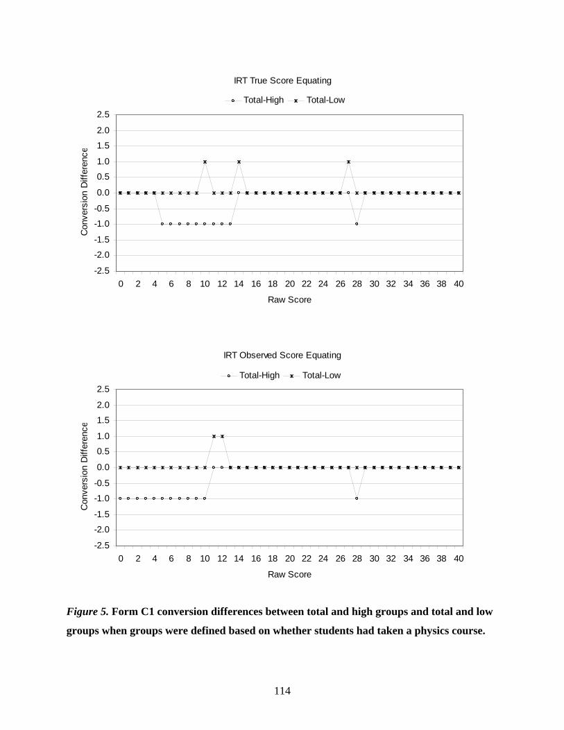
114

Figure 5. Form C1 conversion differences between total and high groups and total and low

groups when groups were defined based on whether students had taken a physics course.

IRT True Score Equating

-2.5

-2.0

-1.5

-1.0

-0.5

0.0

0.5

1.0

1.5

2.0

2.5

0 2 4 6 8 10 12 14 16 18 20 22 24 26 28 30 32 34 36 38 40

Raw Score

Con

vers

ion

Diff

eren

ce

Total-High Total-Low

IRT Observed Score Equating

-2.5

-2.0

-1.5

-1.0

-0.5

0.0

0.5

1.0

1.5

2.0

2.5

0 2 4 6 8 10 12 14 16 18 20 22 24 26 28 30 32 34 36 38 40

Raw Score

Con

vers

ion

Diff

eren

ce

Total-High Total-Low

115

Figure 6. Form B2 conversion differences between total and high groups and total and low

groups when groups were defined based on whether students had taken a physics course.

IRT True Score Equating

-2.5-2.0-1.5-1.0-0.50.00.51.01.52.02.5

0 2 4 6 8 10 12 14 16 18 20 22 24 26 28 30 32 34 36 38 40

Raw Score

Con

vers

ion

Diff

eren

ceTotal-High Total-Low

IRT Observed Score Equating

-2.5-2.0-1.5-1.0-0.50.00.51.01.52.02.5

0 2 4 6 8 10 12 14 16 18 20 22 24 26 28 30 32 34 36 38 40

Raw Score

Con

vers

ion

Diff

eren

ce

Total-High Total-Low

Equipercentile Equating

-2.5-2.0-1.5-1.0-0.50.00.51.01.52.02.5

0 2 4 6 8 10 12 14 16 18 20 22 24 26 28 30 32 34 36 38 40

Raw Score

Con

vers

ion

Diff

eren

ce

Total-High Total-Low

116

Figure 7. Form B1 conversion differences between total and high groups and total and low

groups when groups were defined based on students’ self-reported GPA in science courses.

IRT True Score Equating

-2.5-2.0-1.5-1.0-0.50.00.51.01.52.02.5

0 2 4 6 8 10 12 14 16 18 20 22 24 26 28 30 32 34 36 38 40

Raw Score

Con

vers

ion

Diff

eren

ceTotal-High Total-Low

IRT Observed Score Equating

-2.5-2.0-1.5-1.0-0.50.00.51.01.52.02.5

0 2 4 6 8 10 12 14 16 18 20 22 24 26 28 30 32 34 36 38 40

Raw Score

Con

vers

ion

Diff

eren

ce

Total-High Total-Low

Equipercentile Equating

-2.5-2.0-1.5-1.0-0.50.00.51.01.52.02.5

0 2 4 6 8 10 12 14 16 18 20 22 24 26 28 30 32 34 36 38 40

Raw Score

Con

vers

ion

Diff

eren

ce

Total-High Total-Low

117

Figure 8. Form C1 conversion differences between total and high groups and total and low

groups when groups were defined based on students’ self-reported GPA in science courses.

IRT True Score Equating

-2.5

-2.0

-1.5

-1.0

-0.5

0.0

0.5

1.0

1.5

2.0

2.5

0 2 4 6 8 10 12 14 16 18 20 22 24 26 28 30 32 34 36 38 40

Raw Score

Con

vers

ion

Diff

eren

ceTotal-High Total-Low

IRT Observed Score Equating

-2.5

-2.0

-1.5

-1.0

-0.5

0.0

0.5

1.0

1.5

2.0

2.5

0 2 4 6 8 10 12 14 16 18 20 22 24 26 28 30 32 34 36 38 40

Raw Score

Con

vers

ion

Diff

eren

ce

Total-High Total-Low

118

Figure 9. Form B2 conversion differences between total and high groups and total and low

groups when groups were defined based on students’ self-reported GPA in science courses.

IRT True Score Equating

-2.5-2.0-1.5-1.0-0.50.00.51.01.52.02.5

0 2 4 6 8 10 12 14 16 18 20 22 24 26 28 30 32 34 36 38 40

Raw Score

Con

vers

ion

Diff

eren

ceTotal-High Total-Low

IRT Observed Score Equating

-2.5-2.0-1.5-1.0-0.50.00.51.01.52.02.5

0 2 4 6 8 10 12 14 16 18 20 22 24 26 28 30 32 34 36 38 40

Raw Score

Con

vers

ion

Diff

eren

ce

Total-High Total-Low

Equipercentile Equating

-2.5-2.0-1.5-1.0-0.50.00.51.01.52.02.5

0 2 4 6 8 10 12 14 16 18 20 22 24 26 28 30 32 34 36 38 40

Raw Score

Con

vers

ion

Diff

eren

ce

Total-High Total-Low

119

The consistency of the equating results obtained from the subgroups and equating

methods can be examined by looking at the percentages of examinees at different raw score

points. Tables 6 and 7 present the percentages of examinees and equated raw scores at three

number-right (raw) score points, 19, 23, and 27, under the three equating and three grouping

methods for Forms B1 and B2, respectively. The reason for choosing these three raw score

points was that about 75% of the examinees scored 19 or higher, about 50% scored 23 or higher,

and about 25% scored 27 or higher.

Table 6

Percentages of Examinees at Three Raw Score and Equated Raw Score Points Based on

Different Equating Methods and Grouping Variables for Form B1

Total group IRT true score IRT observed score Equipercentile Raw N % Total Low High Total Low High Total Low High

Composite score 19 162 4.75 19 19 19 19 19 19 19 19 19 23 200 5.86 23 24 23 23 23 23 24 23 24 27 184 5.39 28 28 28 28 28 28 28 28 28

Physics course taken 19 162 4.75 18 19 19 19 18 19 19 18 20 23 200 5.86 23 24 23 23 23 24 24 23 24 27 184 5.39 28 28 27 28 28 28 28 28 28

Self-reported GPA 19 162 4.75 19 19 18 19 19 19 19 19 19 23 200 5.86 23 24 23 23 24 23 24 24 24 27 184 5.39 28 28 28 28 28 28 28 28 28

The subgroup equated raw scores that are different from the total group scores are bolded

in Tables 6 and 7. Table 6 shows that for Form B1 under the IRT true score equating method at a

raw score point of 23, the equating results would be the same for the total and high groups.

However, for the low groups based on the average test center composite scores, physics course

taken, and self-reported GPA, the equated raw score was one point higher. About 6% of the

examinees would be affected if the equating results obtained from the low group were used.

120

Table 7

Percentages of Examinees at Three Raw Score and Equated Raw Score Points Based on

Different Equating Methods and Grouping Variables for Form B2

Total group IRT true score IRT observed score Equipercentile Raw N % Total Low High Total Low High Total Low High

Composite score 19 147 5.58 19 19 19 19 19 19 19 19 19 23 155 5.89 24 24 24 24 24 24 24 24 24 27 130 4.94 28 28 29 28 28 28 28 28 28

Physics course taken 19 147 5.58 19 18 20 19 19 20 19 19 20 23 155 5.89 24 23 25 24 23 25 24 23 24 27 130 4.94 28 28 29 28 28 29 28 28 29

Self-reported GPA 19 147 5.58 19 19 19 19 19 20 19 19 19 23 155 5.89 24 23 24 24 23 24 24 24 24 27 130 4.94 28 28 29 28 28 29 28 28 29

Table 6 also states that for Form B1 under the IRT observed score equating method at a

raw score point of 19 when the groups were divided based on if examinees had taken a physics

course, the equated raw score was one point lower if the low groups’ equating results were used

than if the total group or the high group results were used. About 5% of the total examinees

would be affected by using the equating results from the low groups. Under the equipercentile

equating method, the use of the equating results from subgroups would also affect about 5% to

6% of the examinees at raw scores of 19 and 23.

A raw score of 27 for Form B1 would convert to an equated raw score of 28 when the

IRT observed score and the equipercentile equating methods were used. However, under the IRT

true score equating method, a raw score of 27 only corresponded to an equated raw score of 27

(the bolded value in Table 6) if the high physics-course-taken group’s equating result was used.

About 5.39% (184) examinees would be affected.

Similarly, Table 7 shows that for Form B2 some examinees’ scores could be affected

using the equating results obtained from subgroups, especially when subgroups were obtained

based on physics course taken or self-reported GPA.

121

Effect on Equated Raw Scores’ Mean

Figures 10, 11, and 12 present the mean equated raw scores for the total groups when

different conversions obtained from the subgroups were applied, thus providing a common basis

for examining equated raw score mean and standard deviation differences. The means from the

conversions using the low and high average test center composite score groups were similar.

However, the means from the conversions when the low and high groups were based on whether

examinees had taken a physics course were different, especially for Form B2. The use of the high

GPA group resulted in lower mean equated raw scores for Forms B1 and C1, but higher mean

equated raw scores for Form B2. The pattern of the equated raw score means between high and

low groups is similar for Forms B1 and C1.

Measures of Group Invariance

Dorans and Feigenbaum (1994) used the notion of a score DTM to address the issue of

how large an REMSD would raise concern about the equitability of two tests. The practice of

ignoring differences of less than half a score unit has been used for SAT equating decisions since

the mid-1980s (Dorans & Feigenbaum). The SAT scale is a 200-to-800 scale with 10 points as

an increment score unit. The DTM depends on the reporting scale of a particular testing program:

A difference between equating results larger than a half score unit means a difference that

matters. In this study, the same criterion was used to evaluate the value of REMSD. To compare

REMSD with a DTM, the DTM needs to be standardized. For each form, the DTM was obtained

by dividing 0.5 (half an equated raw score point in the present study) by the standard deviation of

the form. Table 8 contains the REMSD of Forms B1, C1, and B2 when examinee groups were

divided based on different criteria. The DTM for Forms B1, C1, and B2 is 0.0847, 0.0719, and

0.0832, respectively. The REMSD for all the forms was smaller than the DTM when the groups

were divided using a third form composite score (i.e., score on Form X). The REMSD was larger

than the DTM when the groups were obtained based on whether examinees had taken a physics

course, except for Form C1. When the sum of self-reported science GPA was used to divide

groups, the REMSD for Form B2 across all the equating methods was larger than the DTM.

Figures 13, 14, and 15 present how the RMSD varies across the score points. Figure 13

displays the RMSD for Form B1, which shows that the subgroup of examinees who had taken a

physics course had a RMSD different from 0 at most of the score points, while the two other

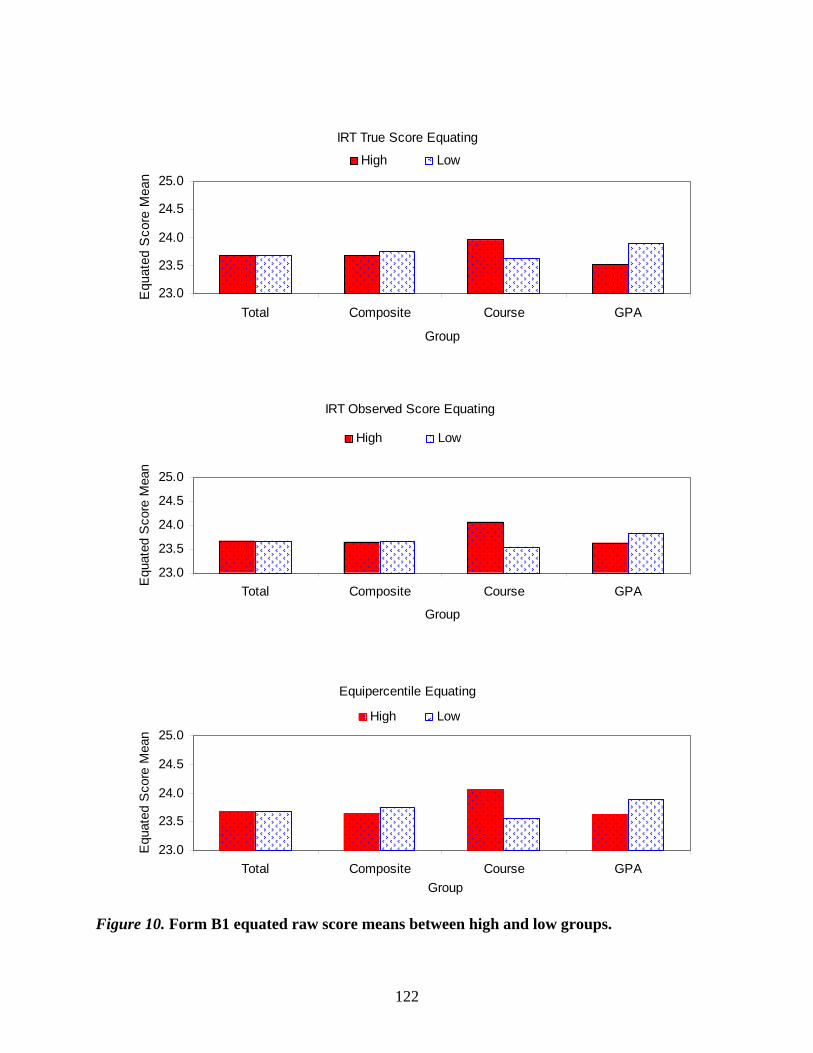
122

Figure 10. Form B1 equated raw score means between high and low groups.

IRT True Score Equating

23.0

23.5

24.0

24.5

25.0

Total Composite Course GPA

Group

Equ

ated

Sco

re M

ean

High Low

IRT Observed Score Equating

23.0

23.5

24.0

24.5

25.0

Total Composite Course GPA

Group

Equ

ated

Sco

re M

ean

High Low

Equipercentile Equating

23.0

23.5

24.0

24.5

25.0

Total Composite Course GPAGroup

Equ

ated

Sco

re M

ean

High Low

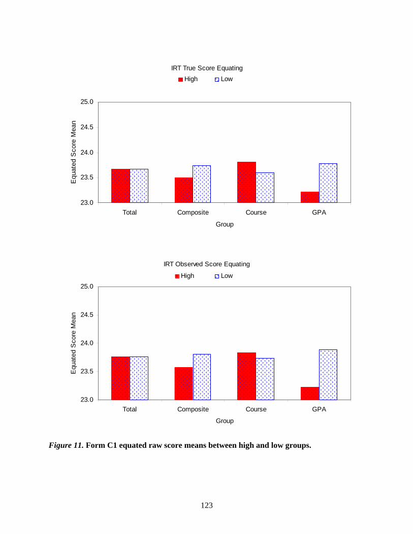
123

Figure 11. Form C1 equated raw score means between high and low groups.

IRT True Score Equating

23.0

23.5

24.0

24.5

25.0

Total Composite Course GPA

Group

Equ

ated

Sco

re M

ean

High Low

IRT Observed Score Equating

23.0

23.5

24.0

24.5

25.0

Total Composite Course GPA

Group

Equ

ated

Sco

re M

ean

High Low

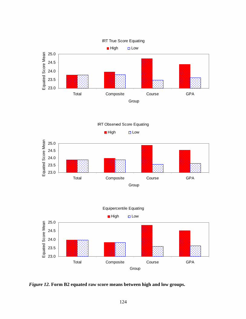
124

Figure 12. Form B2 equated raw score means between high and low groups.

IRT True Score Equating

23.0

23.5

24.0

24.5

25.0

Total Composite Course GPA

Group

Equ

ated

Sco

re M

ean

High Low

IRT Observed Score Equating

23.0

23.5

24.0

24.5

25.0

Total Composite Course GPA

Group

Equ

ated

Sco

re M

ean

High Low

Equipercentile Equating

23.0

23.5

24.0

24.5

25.0

Total Composite Course GPAGroup

Equ

ated

Sco

re M

ean

High Low

125

Figure 13. RMSD of Form B1 across different equating methods.

IRT True Score Equating

-0.050.000.050.100.150.20

0 5 10 15 20 25 30 35 40

Raw Score

RM

SD

Composite Score Group Course Taken Group GPA Group

IRT Observed Score Equating

-0.050.000.050.100.150.20

0 5 10 15 20 25 30 35 40

Raw Score

RM

SD

Composite Score Group Course Taken Group GPA Group

Equipercentile Equating

-0.050.000.050.100.150.20

0 5 10 15 20 25 30 35 40

Raw Score

RM

SD

Composite Score Group Course Taken Group GPA Group

126

Figure 14. RMSD of Form C1 across different equating methods.

IRT True Score Equating

-0.05

0.00

0.05

0.10

0.15

0.20

0 5 10 15 20 25 30 35 40

Raw Score

RM

SD

Composite Score Group Course Taken Group GPA Group

IRT Observed Score Equating

-0.05

0.00

0.05

0.10

0.15

0.20

0 5 10 15 20 25 30 35 40

Raw Score

RM

SD

Composite Score Group Course Taken Group GPA Group

127

Figure 15. RMSD of Form B2 across different equating methods.

IRT True Score Equating

-0.050.000.050.100.150.20

0 5 10 15 20 25 30 35 40

Raw Score

RM

SD

Composite Score Group Course Taken Group GPA Group

IRT Observed Score Equating

-0.050.000.050.100.150.20

0 5 10 15 20 25 30 35 40

Raw Score

RM

SD

Composite Score Group Course Taken Group GPA Group

Equipercentile Equating

-0.050.000.050.100.150.20

0 5 10 15 20 25 30 35 40

Raw Score

RM

SD

Composite Score Group Course Taken Group GPA Group

128

Table 8

REMSD of Forms B1, B2, and C1 Across Different Subgroups

Equating method Test form IRT true score IRT observed score Equipercentile

Composite score B1 0.0675 0.0664 0.0622 B2 0.0705 0.0628 0.0641 C1 0.0548 0.0411

Physics course taken B1 0.0949 0.0975 0.0875 B2 0.1103 0.1237 0.1148 C1 0.0552 0.0560

Self-reported GPA B1 0.0557 0.0605 0.0721 B2 0.0954 0.0936 0.0841 C1 0.0726 0.0655

subgroups showed a RMSD different from 0 at some of the score points across all the equating

methods. Figure 15 shows that a similar pattern of RMSD was found for Form B2.

Conclusion

Group invariance is an important property for equatings to attempt to achieve. Successful

equating adjusts for differences in the difficulty of test forms, and the resulting equated scores

have the same meaning regardless of when or to whom the test was administered. It is, therefore,

important to evaluate whether the equating result is the same regardless of the group of

examinees used to conduct the equating. Subgroups can be defined by various characteristics,

such as gender or ethnicity. Harris and Kolen (1986) examined group independence using

subgroups based on ability, where ability was defined based on self-reported overall GPA. They

found the equating methods studied to be reasonably robust to group differences. The present

study also looked at subgroups based on ability, but defined ability as related to test content (i.e.,

self-reported GPA for science courses, rather than overall GPA). This study attempted to

investigate the consistency of equating results across groups of examinees with different abilities

in terms of the average of the test center composite scores, physics-courses-taken background,

and self-reported science GPA.

129

Several findings are noteworthy. First, the average science equated raw scores were not

very different for the high and low groups assigned according to the average of the test center

composite scores. The conversions derived from the two subgroups were similar at the middle

part of the raw score range. When the conversions were applied to the total group, the mean of

the equated raw score was similar. However, the average science equated raw scores were

different for the high and low groups assigned according to whether the examinees had taken a

physics course and self-reported science course GPAs. The conversions from these two

subgroups varied at most of the raw score points. Nevertheless, the differences were generally

one equated raw score point.

Second, the equated raw scores from the equating of examinees who had taken a physics

course were usually higher than the equated raw scores from the total group. However, the

conversion from the low group was either the same or lower than the conversion from the total

group.

Third, the findings were usually consistent across the IRT and classical equating

methods, and they were also consistent across two different forms within the first year. Some of

the findings were similar across different years, but others were not. REMSD and RMSD(x)

results also show that the conversions obtained from the subgroups based on whether examinees

had taken a physics course had larger differences than the conversions from the total group.

The findings of this study indicate that if the subgroups’ abilities are related to

performance on the science test (e.g., examinees’ self-reported science courses GPA or if

examinees had taken a physics course) then equating results are more group sensitive. Similar

results are reported in Cook and Petersen (1987).

This study was experimental and did not use the procedures associated with the

operational science test, that is, a different linkage plan, score scale, and subgroups were used in

this study. The analyses conducted in this study should be reevaluated with different tests and

different grouping criteria (e.g., assigning examinees to subgroups based on gender, ethnic

background, or geographic region). The results of this study showed that the differences between

the equating results obtained from the total group and subgroups among the three equating

methods were small; however, caution should be taken when generalizing the findings to

situations that were not considered in this study.

130

Future study may use the bootstrap procedure to compute the standard error of equating

in order to examine if the differences obtained in this study are due to random error. In addition,

the issue of group invariance should be explored in situations where the nature of the data

requires the use of a different IRT model (e.g., a polytomous IRT model).

The Role of the Anchor Test in Achieving Population

Invariance Across Subpopulations and Test Administrations

Neil J. Dorans, Jinghua Liu, and Shelby Hammond

ETS, Princeton, NJ

131

Abstract

This exploratory study was built upon research that spans three decades. The massive Petersen,

Marco, and Stewart (1982) study is a major empirical investigation of the efficacy of different

equating methods under a variety of conditions. The matched sample studies reported in Dorans

(1990) examined how different equating methods performed across samples that were selected in

different ways. The population invariance studies that built upon initial work by Dorans and

Holland (2000) have examined whether different equating methods worked as well for males and

females and across other groups. The current study confirmed findings of earlier research and

clarified the role of population invariance studies in assessing equating results. Results showed

that an inappropriate anchor (e.g., a math anchor for equating verbal test scores) did not produce

sound score equatings, but it did seem to yield a strong degree of invariance across

subpopulations. An appropriate anchor (e.g., a verbal anchor for equating verbal test scores)

produced slightly more subpopulation sensitive results and equating results that are consistent

with previous findings: solid equating results under small ability differences and a divergence of

equating results for different methods under large ability differences. Lack of population

invariance of equating results can be taken as evidence that a linking is not an equating. The

existence of invariance, however, does not necessarily mean that the score interchangeability

sought by equating has been achieved.

Key words: Test equating

132

Acknowledgments

The authors thank Linda Cook, Daniel Eignor, and Skip Livingston for their helpful reviews. The

opinions expressed are those of the authors. An earlier version of this paper was presented at the

annual meeting of the National Council on Measurement in Education (NCME) held April 13 to

15, 2004, in San Diego, CA.

133

Overview

For decades, scores have been linked such that statistics associated with their

distributions have been matched. While much time and effort has been given to how to collect

data to equate test scores and what methods to use for score equating, much less attention has

been given to whether or not the process has achieved its stated goal. Lord (1980, chap. 13)

provided guidelines for evaluating whether or not equating test scores makes sense.

Unfortunately, Lord’s valuable perspective on score equating is often reduced to a restatement of

his Theorem 13.3.1 (Lord, p. 198): Equating is either impossible or unnecessary. This

restatement has had little impact on practice. For a variety of reasons, alternate forms of tests

have been produced, data have been collected, and equating procedures have been applied with

the expectation that interchangeable scores would be produced.

Dorans and Holland (2000) revisited Lord’s guidelines, modified the framework, and

proposed indices that can be used to evaluate how much a linking deviates from the ideal of

perfect equatability. Population invariance plays a central role in assessing equatability. Tests are

equatable to the extent that the same equating function is obtained across significant

subpopulations, such as males or females. The Spring 2004 special issue of Journal of

Educational Measurement (Dorans, 2004a) contained a collection of articles on the sensitivity of

equating to subpopulations, which are typically defined by examinee characteristics or

demographic variables such as gender, ethnicity/race, or geographical region.

At the 1989 annual meeting of the American Educational Research Association (AERA)

a symposium titled Selecting Samples for Equating: To Match or Not to Match focused on how

different equating methods perform under different sampling conditions: representative or

matched samples. Matching of equating samples, which entails subsampling to produce identical

score distribution on the anchor test, initially was viewed as a potential solution to the chronic

problem of divergent equating results obtained under different equating methods when data are

collected in an anchor test design in which the old form and new form equating samples differ

substantially (Lawrence & Dorans, 1988). That symposium evolved into a special issue of

Applied Measurement in Education (Dorans, 1990). A follow-up study by Wright and Dorans

(1993) synthesized the studies in that symposium and illustrated the importance of having the

anchor test reflect the sampling process that lead to old and new form samples.

134

In this study, we examine the role of anchor tests in achieving population invariance of

equatings across subpopulations and in compensating for sample selection effects. We use SAT®

data for the purpose of illustration. The second section reviews previous research that has a direct

bearing either on the examination of the role of the anchor in compensating for sample selection

effects or on the invariance of equatings across subpopulations. The third section on data

development describes the SAT equating procedure and briefly describes the procedure used to

simulate populations. The fourth section discusses the equating methods studied here and their

relationships. The fifth section describes the various combinations of equating methods, anchor

tests, and subpopulations examined in this study. The sixth section presents the results of the

study, and the seventh section synthesizes these findings.

Background and Purpose

Invariance of Equatings Across Subpopulations

Kolen (2004), in a historical review in the special issue of Journal of Education

Measurement on population invariance (Dorans 2004a), traced the concept of population

invariance in equating and linking from the 1950s to the present. Much of the research that

Kolen summarized occurred since 1980. Central to this body of work is the expectation that

equating should be population invariant, while linking is not expected to be invariant. In addition

to reviewing the literature, Kolen made suggestions for future methodological research on

measures of population sensitivity and for a better understanding of the conditions under which

equatings are sufficiently invariant for practical use.

von Davier, Holland, and Thayer (2004a), in a methodological paper in that special issue,

extended the work on subpopulation invariance done by Dorans and Holland (2000) for the

single population case to the two-population case in which the data are collected on an anchor

test as well as the tests to be equated. Typically the two populations are not equivalent; the

authors refer to this design as the non-equivalent-group anchor test (NEAT) design. In addition,

the authors provided a common statistical framework from which they examined closely two

common observed score equating methods, chained equating, and poststratification. In chained

equating, the tests are linked indirectly through their linkages to a common anchor; in

poststratification, the anchor is used as a poststratification variable to estimate performance on

both tests in a hypothetical population. Poststratification includes what Angoff (1971) and others

135

have called frequency estimation and Tucker equating. These methodological developments are

pertinent to the present paper.

Yang (2004) then examined whether the multiple-choice to composite linking functions

of Advanced Placement Program® (APP

®) exams remain invariant over subgroups by region. The

study focused on two questions: (a) how invariant are cut-scores across regions and (b) whether

the small sample size for some regional groups presents particular problems for assessing linking

invariance. In addition to using the subpopulation invariance indices to evaluate linking

functions, the author also evaluated the invariance of the composite score thresholds for

determining final AP grades. Overall, linkings across regions seemed to hold reasonably well.

Males and females exhibit differential mean score differences on the free-response and

multiple-choice sections. Do these differential mean score differences affect the equatability of

AP scores and the invariance of AP grade assignments across gender groups? Dorans (2004c), in

the last article in the special issue, used the population sensitivity of linking functions to assess

score equity for two AP exams. Score equity assessment was introduced and placed within a

fairness framework that encompasses differential prediction and differential item functioning, as

well as population sensitivity of equating functions. In the examples he looked at, Dorans found

invariance to hold for the calculus exam, but not for the U.S. history exam.

Yin, Brennan, and Kolen (2004) looked closely at the issue of invariance of concordance

results across subgroups, using concordances between ACT scores and scores on the Iowa Tests

of Educational Development in a special issue of Applied Psychological Measurement titled

Concordance (Pommerich & Dorans, 2004). Linear, parallel-linear, and equipercentile methods

were used to conduct concordances for males, females, and the combined group. Gender

invariance was evaluated both graphically and using group invariance statistics, for each linking

method. The different linkage methods were evaluated with respect to group invariance. The

results were also interpreted relative to the degree of content similarity across the linked tests:

Similar content specifications lead to invariance of linear linking functions, while dissimilar

content lead to group-dependent linking functions, especially for the linear methods.

The other papers in this volume provide further examples of how population invariance

can be used to assess whether test scores are equitable or not. von Davier and Wilson (2006, this

volume, pp. 1–28) examine the population invariance of IRT equating for an AP exam. Liu and

Holland (2006, this volume, pp. 29–58) examine the population invariance of parallel-linear

136

linkings across different subpopulations of the Law School Admission Test. Yang and Gao

(2006, this volume, pp. 59–98) look at invariance of linking computer-administered College-

Level Examination Programs® (CLEP®) data across gender groups. Yi, Harris, and Gao (2006,

this volume, pp. 99–129) examine the invariance of IRT equating across different subpopulations

of a science achievement test.

Sensitivity of Anchor Test Equatings to Selection of Equating Samples

A major motivation for the studies reported in Dorans (1990) was to see if it was possible

to improve anchor test equatings via matching on the equating test when the old form and new

form groups were quite dissimilar. Using data from several administrations of the SAT,

Lawrence and Dorans (1990) addressed the sample invariant properties of five anchor test

equating methods across two sampling conditions to see which methods produced the most

consistent results. Among the five equating methods, two were based on the equipercentile

definition of equating: chained and frequency estimation; two were based on the mean-sigma

linear observed score definition: Tucker and Levine; and one was based on a true score

definition, item response theory (IRT) equating. The two sampling conditions were the

representative sample condition and the matched sample condition. In the representative sample

condition, equatings were based on old form and new form samples that differed in ability; in the

new form matched sample condition, the old form sample was selected to match the anchor test

score distribution of the new form sample. Results for the IRT method differed for representative

and matched samples, as did results for the Levine and chained equipercentile methods. Results

based on the Tucker observed score method and frequency estimation equipercentile equating

methods were found to be essentially invariant across representative and new form matched

sample conditions. Results for the five equating methods tended to converge under the new form

matched sample condition. Tentative explanations for the findings were offered.

Eignor, Stocking, and Cook (1990) employed a simulation model to study the invariance

effect. Two independent replications of a sequence of simulations were carried out to evaluate

the performance of four anchor test equating methods (Tucker, Levine, IRT, and chained

equipercentile) under two sampling design conditions, matched and representative. Since the

data were generated according to an IRT model, it was predicted that the IRT method and the

Levine method would be less affected by sample differences, and the results confirmed this

137

finding. The authors advised against matching on equating tests for the IRT, Levine, and chained

equipercentile methods.

Schmitt, Cook, Dorans, and Eignor (1990) examined the results of equating two parallel

editions of an achievement test in biology using different equating methods under different

sampling strategies. In addition to representative samples and new form matched samples, they

studied reference or target matched sampling. The criterion equating was Tucker equating using

representative samples from two populations that were very close in ability. They found that

matching on a set of common items provided greater agreement among the results of the various

equating procedures than was obtained under representative sampling. In addition, for all

equating procedures, the results of equating with samples matched on common item scores

agreed more closely with the criterion equating than did results from representative samples.

Matching to a reference target population produced agreement among methods, but this did not

agree as closely with the criterion equating as matching to the new form on the basis of common

item scores. The equating models least affected by differences in new and old form sample

abilities were the Tucker and Frequency Estimation equipercentile models, and the procedure

most affected by ability differences was the IRT procedure. Cook, Eignor, and Schmitt (1989)

examined one edition of four other achievement tests and failed to replicate the superiority of

matched sample equatings.

Livingston, Dorans, and Wright (1990) examined the five equating methods studied by

Lawrence and Dorans (1990) under two sampling conditions using data specially constructed

from a national administration of the SAT. The criterion equating was based on an equivalent-

groups design equating involving more than 115,000 students taking each of two editions of the

SAT. Much of the inaccuracy in the equatings could be attributed to overall bias. The results for

all equating methods in the matched samples were similar to those for the Tucker and frequency

estimation methods in the representative samples: These equatings made too small an adjustment

for the difference in the difficulty of the test forms. In the representative samples, the chained

equipercentile method showed a much smaller bias. The IRT and Levine equally reliable

methods tended to agree with each other and were inconsistent in the direction of their bias.

This set of papers could be viewed as a psychometric drama about the efficacy of

matching, which swayed from a yes based on the Lawrence and Dorans (1990) study to a

definite no according to Eignor et al. (1990), back to a yes by Schmitt et al. (1990), then back yet

138

again to a no according to Livingston et al. (1990). Kolen (1990) and Skaggs (1990) examined

these articles, synthesized them, posed questions, and discussed their implications for current and

future equating practices. In addition to providing critiques of the individual articles, both Kolen

and Skaggs looked for universal themes that could be extracted from this psychometric drama.

Skaggs (1990) concluded that Tucker and frequency estimation are not affected by

matching on the equating test, while Levine, IRT, and chained equipercentile equating are

affected. Skaggs also pointed out that the conclusions one might draw about the efficacy of

matching depend on the criterion used. If consistency among methods is the criterion, then

matching achieves that consistency. Skaggs raised the issue of multidimensionality and

wondered how it may have affected different methods in the different studies. Finally, he

concluded that researchers need to know more about examinees and how they end up in their

samples.

Kolen (1990) indicated that three general research findings underlie this set of studies.

First, when equivalent groups of examinees are given test forms carefully constructed to measure

the same construct, the equating relationship is invariant with respect to the subpopulation from

which the equating samples are drawn. Second, when an anchor test is used in which the anchor

is a miniature of the total test form and is administered to groups taking the old and new form

that are similar to each other, equating methods tend to give similar results. Third, when an

anchor test is used and the groups taking the old and new forms are quite different, any equating

method may give poor results. Kolen concluded from these studies that matching on the equating

test does not result in more accurate equating. He also stated that matching on other variables is

worthy of future research.

Wright and Dorans (1993) addressed whether we can improve equating results if we

know the variable that accounts for all systematic differences between equating populations and

use it either as an anchor in an anchor test design or as a variable on which to match equating

samples. The sample invariant properties of four anchor test equating methods (Tucker and

Levine linear models and chained and frequency estimation equipercentile models) under three

sampling conditions, representative, matched on equating test, and matched on selection variable

were examined. The selection variable was defined as the variable or set of variables along

which subpopulations differ. The selection variable was the same as that used in Livingston et al.

(1990), namely the anchor score on the test not being equated. For the math score equatings, the

139

verbal anchor was the selection variable; for the verbal score equatings, the math anchor score

was the selection variable. In addition to being used for matching of subpopulations, the

selection variable was also used as an anchor for the four equating methods and compared to

equatings in which the equating test served as the anchor. All equatings were performed with

either real SAT populations or with data drawn from simulated pseudopopulations, which

differed from their original real SAT populations on the basis of the selection variable. Results

showed that matching on the selection variable improved accuracy over matching on the

equating test for all methods. Compared with the representative sample equatings, Tucker and

frequency estimation results improved with matching on the selection variable; chained

equipercentile and Levine results were similar under these two sampling conditions. Results with

the selection variable as an anchor were good for both the Tucker and frequency estimation

methods; chained equipercentile and Levine results were quite unacceptable as anticipated since

use of the selection variables—math scores for the verbal score equatings and verbal scores for

the math score equatings—violated assumptions of these models. The positive results obtained

for use of the selection variable as a matching variable or anchor test (for some methods)

suggested that future research into the reasons test takers elect certain test administrations might

lead to improved test score equating practices. In particular, supplementing the anchor test with

other variables that account for old form and new form differences could improve the accuracy

of equating results.

The present study can be viewed as an extension of the Lawrence and Dorans (1990);

Livingston et al. (1990); and the Wright and Dorans (1993) studies. Instead of selecting samples

or simulating populations on the basis of the verbal equating test score or the math score, we

construct our population with respect to sampling on verbal and math scaled scores

simultaneously to look like actual SAT equating populations. Because of the bivariate selection

used to construct the simulated populations, we examined the Tucker two-anchor equating

method. In addition we crossed the Tucker, chained, and Levine methods with each of three

anchors: verbal equating test, math score, and a composite of math score and verbal equating test

for which the contributions of each, in standard deviation units, was equal. Finally, we examined

the sensitivity of equating to subpopulation for each of the different equating method and anchor

test combinations. The features that distinguish this research from previous research were the

inclusion of population invariance as a criterion for evaluating equatings, the generation of

140

populations via variation along a bivariate surface, and the use of the Tucker two-anchor linking

method.

The Relative Efficacy of Different Equating Methods

Over the past quarter century, equating methods have been pitted against each other to

determine which method would prevail under different conditions. One of the earliest and most

massive of these studies was conducted by Marco, Petersen, and Stewart and reported in several

places, including Petersen, Marco, and Stewart (1982). This empirical study examined linear and

curvilinear methods and observed score and true score methods, ranging from widely used

methods to rather obscure methods. (For a list of the methods studied, see Table 1 in Petersen et

al., 1982, pp. 76–78). They examined different types of content for the internal anchor, ranging

from test-appropriate equating tests to tests measuring different constructs. For example, they

studied equating SAT verbal exams through a verbal equating test, a set of vocabulary items, a

measure of writing ability, or a measure of mathematical ability. Some anchors were external

(did not count towards the score), while others were internal. Anchors also varied in difficulty. In

addition, equating samples were randomly equivalent, similar, or dissimilar in ability.

This massive study produced many results and the authors drew several conclusions. The

conclusions most pertinent to the current research are that anchor tests that are constructed to be

miniatures of the total test work better than other anchor tests and that the Tucker method has

problems when equating samples are dissimilar.

The current study differs in a few significant ways from the Petersen et al. (1982) study.

Only one test is equated, and though it is not equated to itself, it is equated to a different order of

itself. Because the tests to be equated are scrambles of each other, only linear methods are

studied because scramble effects are virtually nonexistent with the SAT. As illustrated below,

different anchors are used across different equating methods. We also examine the population

invariance across males and females for each combination of method and anchor.

Data Development

Equating Design and Equating Methods

SAT I data are used in this study because the tests are very reliable, and the data

collection design is an exemplar for linking forms with the anchor test or non-equivalent-groups

with anchor test (NEAT) design. In the anchor test design, one group takes the old form and

141

another group takes the new form, but the samples are not selected to ensure equivalent test

performance. Ordinarily, the equating data come from different test administrations. Equating or

anchor tests are essential for designs in which the old form and new form samples are not

exchangeable.

In a typical SAT I administration, a new test is administered in two section orders, one is

called the original order while the other is the scrambled order. In this study, we focus on the

verbal test only. The original order is linked back to four old SAT I forms. One of the old forms

was administered at the same time of year as the new form, and we call it the link to the Similar

population. Each of the other three old forms was administered at one of three core

administrations of the SAT that contribute large numbers of scores to the SAT cohort. The three

core forms are used at every equating within a given SAT cohort. In the current study, we name

them as links to the Close, Distant, and Far populations. This multiple-link design, which was

adopted in 1994, has produced stable equatings because it directly acknowledges the important

role that the old form scaling plays in placing a new form on scale. After the equatings are

conducted on the original form and a conversion is produced, the same conversion is usually

applied to the scrambled form if no section-order effects are detected.

We treat the scrambled form as the new form and equate the scrambled order to the

original order via an anchor test design. Three standard methods are studied: Tucker, Levine and

the chained linear methods. Petersen et al. (1982) did not study the chained linear, a method of

indirect equating through concatenated scalings. Three anchors are used for the Tucker, Levine,

and chained methods: the verbal equating test (Va), the math test (MT), and a linear composite

(COMP) anchor that is composed of the Va and MT anchors and that gives equal weight (in

standard deviation units) to the two components. In addition, a bivariate (BiV) anchor with the

Tucker two-anchor design is also employed, making use of the Va and MT anchors. In contrast to

the COMP anchor, which is a one-dimensional linear combination of the Va and MT anchors

defined by the standard deviations of the its components, the BiV anchor is a two-dimensional

response surface.

As will be seen shortly, equating samples are constructed on the basis of the joint

distribution of verbal and math scores. And we examine the population invariance across sons

(males) and daughters (females) of results obtained for each of these 10 combinations (3 × 3 + 1)

of method and anchor.

142

In addition, we performed the mean/sigma equating to equate the scrambled form to the

original form through an equivalent groups design, and this conversion line serves as the

criterion. The large sample size and the spiraling procedure used in the SAT administration

usually yield equivalent groups in one administration. Since the forms to be equated were the

same test in two different section orders, the mean/sigma conversion based on 117,671 examines

in the old form and 115,179 examinees in the new form was very close, a = 1.0039, b = -.2106,

to the identity conversion. As expected, when compared to its curvilinear analogue, this linking

was linear.

Simulated Populations

The three equating methods (Tucker, Levine, and chained) were applied to data from one

actual administration and four simulated administrations. As mentioned above, the actual data on

the scrambled form were used as the new form data. The old form data were constructed from the

original order of the new form to simulate each of the four old form populations in the SAT I

equating design. These data were constructed via sampling with replacement from actual data on

the form in the original order. The data were sampled so as to match the bivariate SAT verbal

(SAT-V), SAT math (SAT-M) distribution observed on each of the four actual old forms. For

example, let P represent one old form administration population. The bivariate distribution of

SAT-V, SAT-M scaled scores on P served as the target distribution for sampling scores from the

actual sample that took the original order of the new form used in this study. This sampling with

replacement occurred four times, one for each of the old form administrations, Similar, Close,

Distant, and Far. The distance implied by these names is the distance between administrations in

terms of average ability as measured by the anchor.

These samples were used as old form samples. In essence, these samples differed from

the original sample on the basis of selection on SAT-V, SAT-M simultaneously. In contrast,

Livingston et al. (1990) constructed populations on the basis of math for verbal equatings, and

Lawrence and Dorans (1990) constructed samples on the basis of the verbal anchor for verbal

equatings. Selection on SAT-V, SAT-M seems to be more realistic as a selection variable.

Table 1 presents the mean differences between the new and old form samples on different

anchors and the correlations between different anchor tests and the total verbal test. Among the

four populations, the mean differences on the verbal anchor were the smallest in the Similar and

in the Close populations. On both the MT anchor and the COMP anchor, the Distant population

143

was the one with the smallest difference, a reflection of the fact that SAT administrations differ

with respect to their verbal and math means in distinct ways. As expected, the correlations

between Va anchor and verbal, composite anchor and verbal, and BiV anchor and verbal were

quite high, and the correlation between math anchor and verbal was lower than all the other three

anchors.

The use of the SAT I equating design enabled us to generate realistic data for which two

of the equatings using verbal anchor were expected to be very tight (i.e., much agreement across

equating methods because of small differences between old and new form samples). One was

expected to be problematic because of large differences, and one was expected to provide

intermediate agreement.

Table 1

Standardized Differences Between New and Old Form Populations and Correlations of

Anchor Tests With Total Verbal Test Across Different Populations

Old form population Ability differences on the anchor tests (new – old) Va MT COMP BiV

(V, M) Similar -.02 .09 .08 (-.02, . 09) Close -.03 .10 .08 (-.03, . 10) Distant -.12 -.05 -.05 (-.12, -.05) Far -.36 -.23 -.30 (-.36, -.23) Correlations between anchor tests with total verbal Va MT COMP BiV Similar 0.89 0.70 0.87 0.90 Close 0.89 0.71 0.87 0.90 Distant 0.89 0.72 0.87 0.91 Far 0.89 0.71 0.87 0.90

Linear Equating Methods

In linear equating, a transformation is found such that scores on X and Y are said to be

equated if they correspond to the same number of standard deviation units above and below the

mean in T, where T is the population in which the equating is performed. When the two forms to

be equated are scrambled versions of each other, it is reasonable to expect a linear equating.

144

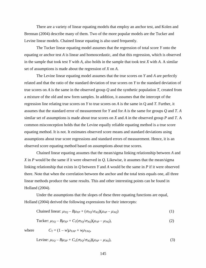
There are a variety of linear equating models that employ an anchor test, and Kolen and

Brennan (2004) describe many of them. Two of the more popular models are the Tucker and

Levine linear models. Chained linear equating is also used frequently.

The Tucker linear equating model assumes that the regression of total score Y onto the

equating or anchor test A is linear and homoscedastic, and that this regression, which is observed

in the sample that took test Y with A, also holds in the sample that took test X with A. A similar

set of assumptions is made about the regression of X on A.

The Levine linear equating model assumes that the true scores on Y and A are perfectly

related and that the ratio of the standard deviation of true scores on Y to the standard deviation of

true scores on A is the same in the observed group Q and the synthetic population T, created from

a mixture of the old and new form samples. In addition, it assumes that the intercept of the

regression line relating true scores on Y to true scores on A is the same in Q and T. Further, it

assumes that the standard error of measurement for Y and for A is the same for groups Q and T. A

similar set of assumptions is made about true scores on X and A in the observed group P and T. A

common misconception holds that the Levine equally reliable equating method is a true score

equating method. It is not. It estimates observed score means and standard deviations using

assumptions about true score regressions and standard errors of measurement. Hence, it is an

observed score equating method based on assumptions about true scores.

Chained linear equating assumes that the mean/sigma linking relationship between A and

X in P would be the same if it were observed in Q. Likewise, it assumes that the mean/sigma

linking relationship that exists in Q between Y and A would be the same in P if it were observed

there. Note that when the correlation between the anchor and the total tests equals one, all three

linear methods produce the same results. This and other interesting points can be found in

Holland (2004).

Under the assumptions that the slopes of these three equating functions are equal,

Holland (2004) derived the following expressions for their intercepts:

Chained linear: μYQ – BμXP + (σYQ/σAQ)(μAP – μAQ) (1)

Tucker: μYQ – BμXP + CT(σYQ/σAQ)(μAP – μAQ), (2)

where CT = (1 – w)ρXAP + wρYAQ,

Levine: μYQ – BμXP + CL(σYQ/σAQ)(μAP – μAQ), (3)

145

where CL = (1 – w)(ρXP/ρAP) + w(ρYQ/ρAQ),

where B is the common slope for the equating of X to Y; μYQ and μXP are observed means on Y in

Q and X in P, respectively; and μAP and μAQ are the means of A in P and Q, while corresponding

standard deviations are represented by σ terms. In (2) for Tucker, ρXAP and ρYAQ are the

correlations of A with X and Y in P and Q, respectively. In (3) for Levine, ρXP and ρAP are the

reliabilities of A and X in P, while ρYQ and ρAQ are the reliabilities of A and Y in Q. In both (2)

and (3), w is the weight assigned to P to create the synthetic population T = wP +

(1 – w)Q.

Note that w does not appear in the expression for chained in (1). von Davier et al. (2004a)

found Tucker to be relatively insensitive to the choice of w. Note if the correlation between

anchor and total test score is 1, all three methods converge to the same equation. This is obvious

in (2) for Tucker, where the term CT become 1. In (3), a perfect anchor test and total test score

correlation implies perfect reliability for X, Y, and A, and so CL also becomes 1. From the

perspective of the Tucker model, chained linear assumes a perfect correlation and from the

perspective of the Levine model, which is rooted in classical test theory, the perfect correlation

implies perfect reliabilities. From a classical test theory perspective, the chained model seems

implausible and the Tucker model insensitive to true score theory. How do the models work in

practice? Holland (2004) demonstrated from the equations above that

CT < 1 < CL,

which means that Tucker will tend to adjust scores less than chained, which will adjust scores

less than Levine. As the correlation between anchor and total drops, Tucker will adjust less and

less, while Levine will adjust more and more. In essence the Tucker model discounts the

information in the anchor as this correlation drops, while Levine makes bigger and bigger

adjustments because differences on the anchor are viewed as attenuated more and more by

reliability. In contrast, chained linear ignores all bivariate information and sets means and

standard deviations equal.

In addition to these three univariate anchors, we used the Tucker two-anchor linking

method described in Angoff (1971). The two anchors are Va and MT. The assumptions for this

method are extensions of the Tucker one-anchor method to a case in which there are two anchors

instead of one. The Tucker two-anchor model assumes that the regression of total score Y onto

146

the anchor test surface (Va, MT) is linear and homoscedastic, and that this regression, which is

observed in the sample that took test Y with (Va, MT), also holds in the sample that took test X

with (Va, MT). A similar set of assumptions is made about the regression of X on (Va, MT).

Equatings Performed and Discrepancy Indices

Equatings Performed

Although it is dwarfed by the massive groundbreaking equating research performed by

Petersen et al. (1982), the number of equatings performed for the present study is very large.

Within each of the four simulated administration populations, three equating methods (Tucker,

Levine, and chained linear) were crossed with three types of anchors (verbal equating test, math

score, and a composite of math score and verbal equating test score). In addition, the Tucker

two-anchor method was conducted with the bivariate anchor. Further, for purposes of checking

for invariance across gender groups, equatings were performed with all the data (Population),

Daughters-only, and Sons-only. We use Sons and Daughters because it is the most descriptive of

the test takers, albeit nonstandard terminology. Male and female is too clinical. Some of the

males are boys, others are men, most are in between. Likewise for girls and women. In contrast,

all have been and always will be a son or daughter.

Within each of the four simulated populations, there were (3 × 3 + 1) × 3 = 30 equatings

performed. Across four simulated populations, that yields 4 × 30 = 120 equatings. Finally, the

criterion large sample equating brought the total number of equatings to 121.

The advantage to using linear equating is that most useful information can be

summarized in terms of the slopes and intercepts of these equatings or functions of these slopes

and intercepts. Table 2 contains the slope and intercepts associated with each of the 30 equatings

linked to the Similar population. Table 3 contains the same information for the Close population.

Table 4 contains the results for the Distant population, and Table 5 contains the results for the

Far population. Within each table are results for each of the three methods for each of the three

anchors across each of the two subpopulations, Daughters and Sons, and for the population.

Each table has two parts, a listing of slopes and intercepts (for Population, Sons, and

Daughters), and two kinds of invariance statistics, invariance as % of score ranges and invariance

as REMSD, which are described in the next section.

147

Discrepancy Indices

This research looks at two issues and their interrelationship. First, we are interested in

studying whether or not different combinations of equating methods and anchors are invariant

across gender groups and whether this invariance is influenced by the degree to which the anchor

test needs to make an adjustment before equating. Second, we are interested in which of the

combinations of equating methods and anchors captures truth, as defined by the large sample

equivalent groups linear equating, across the different simulated populations. The indices we use

to examine these issues are also related.

The population invariance measures are defined in Dorans and Holland (2000) and

particularly in von Davier et al. (2004b) for the anchor test or NEAT data collection design. The

Dorans and Holland measure, RMSD(x) is then defined as

RMSD (x) =

2[ ( ) ( )]jj P P

j

YP

w e x e x

σ

−∑,

where is the equating function in the jth subpopulation, is the equating function in

the population, and σ

( )e xjP ( )e xP

YP is the variance of Y in P. At each X-score, RMSD(x) is the root mean

squared difference (RMSD) between the linking functions computed on each subpopulation and

the linking function computed on the population, P. RMSD(x) is standardized by dividing by the

standard deviation of Y on P so that it is a type of effect size, and its units are percentages of the

Y-standard deviation on P. In this study, both standardized and unstandardized RMSD are used.

As demonstrated by von Davier et al. (2004a), different equating methods have different

population linking functions and different population standard deviations. This fact complicates

comparisons across methods in the NEAT design as compared to the nonanchor test designs in

which there is only one type of linear equating and one type of curvilinear equating in the

population.

To obtain a single number summarizing the values of RMSD(x), Dorans and Holland

(2000) introduced a summary measure by averaging over the distribution of X in P before taking

the square root in RMSD(x). This is the root expected mean squared difference (REMSD):

2 2{ [ ( ) ( )] } {[ ( ) ( )] }REMSD

jP j P P j P P Pj j

YP YP

E w e X e X w E e X e X

σ σ

− −= =

∑ ∑j

148

In addition to using these measures for each of the three linear equating methods, we

make use of the simplicity afforded by the linearity of the equating lines. In particular, we note

that the difference in a criterion or target equating line, Pe , and the jth subpopulation equating

line, jPe , is

( )* (j jDiff B B X I I= − + − )

where B and I are the slope and intercept for the population equating line. A case could be made,

in the absence of more pertinent information about the reporting score scale, that any Diff > -.5

or < .5 is not worth noticing because it is less than half a raw score point. Because of the linear

nature of the equating, we can easily solve for the X values for which Diff < -.5 and Diff > .5 via

( )j

j

Diff I IX

B B− −

=−

by substituting -.5 and then .5 into the equation. REMSD and these values of X at which the lines

began to diverge by a potentially meaningful amount were calculated for each equating method.

A measure of invariance that is independent of the number of examinees at each score level can

be obtained by computing the percentage of the nonchance raw score range for which the

difference between the subpopulation conversion and the total population conversion is between

-.5 and +.5. We computed these percentages for both gender groups and then averaged them

across gender groups to get a combined percentage.

In addition to studying population invariance, we examined the ability of different

combinations of equating method and anchor to properly adjust for population differences and

recreate the target equating line. We computed the root expected squared difference (RESD)

statistic, which is

RESD(x) =

2[ ( ) ( )]s m cs

YP

f e x e x

σ

−∑,

to evaluate how each of these equating method/anchor test combinations ( ), fits the target

equating line at each point. RESD weights by the relative frequency of X scores, f

me

s, in the full

population. It is the same statistic used by Petersen et al. (1982) in their research. We also use the

149

bias statistic employed by Petersen et al. as another basic measure of accuracy. In each case

examined, the large sample linear equating of X to Y, e , was our target criterion equating. c

Results

Population Invariance Across Gender Groups

Table 2 contains the invariance results for the Similar population. Here the standardized

difference between new form group and old form group in verbal anchor scores was -.02.

Reading from the bottom up, we see that overall population invariance across gender is met

reasonably well in this population, as indicated by standardized REMSD values of .01 and .02

across different combinations of anchor and equating method. When we look at invariance as a

percentage of score range (i.e., the proportion of nonnegative raw score points for which the

difference between the gender-specific conversion and the population conversion was less than

half a raw score point in absolute value) we see that the equatings making use of the verbal

equating test are more sensitive to subpopulation (invariant over 73% of score range) than the

equatings making use of the math and composite anchors, or the bivariate anchor.

Table 2

Invariance Results for Three Linear Equating Methods in the Similar Population S

Tucker

BiV Tucker

Va

Levine Va

Chained Va

Tucker MT

Levine MT

Chained MT

Tucker COMP

Levine COMP

Chained COMP

Population Slope 1.02 1.01 1.01 1.01 1.04 1.06 1.06 1.05 1.05 1.06 Intercept -0.07 -0.23 -0.25 -0.25 0.34 0.00 0.06 0.15 0.03 0.00

Sons Slope 1.03 1.02 1.02 1.02 1.05 1.07 1.06 1.05 1.06 1.06 Intercept -0.71 -1.01 -1.01 -1.02 -0.19 -0.34 -0.31 -0.35 -0.41 -0.43

Daughters Slope 1.01 1.00 1.00 1.00 1.03 1.05 1.05 1.04 1.05 1.05 Intercept 0.41 0.39 0.39 0.37 0.73 0.30 0.38 0.50 0.34 0.29

Invariance as % of Score Range Sons 78% 66% 65% 65% 97% 100% 100% 100% 100% 100% Daughters 100% 80% 80% 80% 100% 100% 99% 100% 100% 100% Combined 89% 73% 73% 73% 98% 100% 99% 100% 100% 100%

Invariance as REMSD Raw score 0.34 0.42 0.42 0.42 0.21 0.18 0.18 0.24 0.23 0.23 SD score 0.02 0.02 0.02 0.02 0.01 0.01 0.01 0.01 0.01 0.01

What happens in the simulated population that is close to the new form population with

standardized difference of -.03 in verbal anchor scores? These results are presented in Table 3.

150

The results for the Close population are similar to those for the previous Similar population.

Standardized REMSD values of .01 and .02 indicate invariance across subpopulations. Strangely

enough, the results for the equatings using the verbal equating test are once again less invariant

than those using the bivariate anchor. They are also less invariant than the equatings using the

other two anchors (MT and COMP), where no differences between either the gender-based or

total conversion exceed .5 in absolute value within the nonnegative raw score range.

Table 3

Invariance Results for Three Linear Equating Methods in the Close Population C

Tucker

BiV Tucker

Va

Levine Va

Chained Va

Tucker MT

Levine MT

Chained MT

Tucker COMP

Levine COMP

Chained COMP

Population Slope 1.01 1.00 1.01 1.01 1.02 1.06 1.05 1.04 1.05 1.05 Intercept 0.34 0.10 -0.05 -0.01 1.12 0.68 0.76 0.71 0.54 0.49

Sons Slope 1.02 1.01 1.02 1.02 1.03 1.06 1.05 1.04 1.05 1.05 Intercept -0.24 -0.65 -0.79 -0.75 0.69 0.52 0.56 0.31 0.21 0.18

Daughters Slope 1.00 1.00 1.00 1.00 1.02 1.05 1.04 1.03 1.04 1.05 Intercept 0.77 0.68 0.53 0.57 1.42 0.85 0.95 0.99 0.76 0.70

Invariance as % of Score Range Sons 86% 68% 69% 69% 100% 100% 100% 100% 100% 100% Daughters 100% 84% 85% 85% 100% 100% 100% 100% 100% 100% Combined 93% 76% 77% 77% 100% 100% 100% 100% 100% 100%

Invariance as REMSD Raw score 0.32 0.41 0.40 0.40 0.18 0.14 0.14 0.21 0.19 0.19 SD score 0.02 0.02 0.02 0.02 0.01 0.01 0.01 0.01 0.01 0.01

Table 4 contains the invariance results for population Distant, in which the ability

difference is -.12 in standardized units. The results with the verbal equating test are not as

invariant as those for the less appropriate COMP anchor or for the even more inappropriate MT

anchor. For the verbal equating and math anchor tests, Levine and chained linear methods

provide less invariant results than the Tucker method. Of the anchor tests, the COMP anchor

clearly provides the most invariant results with REMSD values of .01 and combined percent

invariant ranges of at least 95%. The results from Tucker with MT anchor are surprisingly

invariant as well, as are the results of the Tucker with a BiV anchor, both of which have

combined percent invariant ranges of 89%.

151

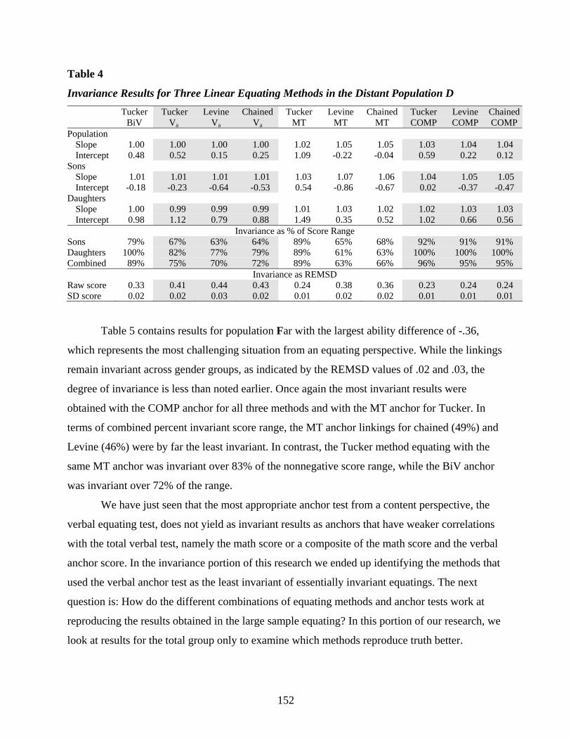
Table 4

Invariance Results for Three Linear Equating Methods in the Distant Population D

Tucker

BiV Tucker

Va

Levine Va

Chained Va

Tucker MT

Levine MT

Chained MT

Tucker COMP

Levine COMP

Chained COMP

Population Slope 1.00 1.00 1.00 1.00 1.02 1.05 1.05 1.03 1.04 1.04 Intercept 0.48 0.52 0.15 0.25 1.09 -0.22 -0.04 0.59 0.22 0.12

Sons Slope 1.01 1.01 1.01 1.01 1.03 1.07 1.06 1.04 1.05 1.05 Intercept -0.18 -0.23 -0.64 -0.53 0.54 -0.86 -0.67 0.02 -0.37 -0.47

Daughters Slope 1.00 0.99 0.99 0.99 1.01 1.03 1.02 1.02 1.03 1.03 Intercept 0.98 1.12 0.79 0.88 1.49 0.35 0.52 1.02 0.66 0.56

Invariance as % of Score Range Sons 79% 67% 63% 64% 89% 65% 68% 92% 91% 91% Daughters 100% 82% 77% 79% 89% 61% 63% 100% 100% 100% Combined 89% 75% 70% 72% 89% 63% 66% 96% 95% 95%

Invariance as REMSD Raw score 0.33 0.41 0.44 0.43 0.24 0.38 0.36 0.23 0.24 0.24 SD score 0.02 0.02 0.03 0.02 0.01 0.02 0.02 0.01 0.01 0.01

Table 5 contains results for population Far with the largest ability difference of -.36,

which represents the most challenging situation from an equating perspective. While the linkings

remain invariant across gender groups, as indicated by the REMSD values of .02 and .03, the

degree of invariance is less than noted earlier. Once again the most invariant results were

obtained with the COMP anchor for all three methods and with the MT anchor for Tucker. In

terms of combined percent invariant score range, the MT anchor linkings for chained (49%) and

Levine (46%) were by far the least invariant. In contrast, the Tucker method equating with the

same MT anchor was invariant over 83% of the nonnegative score range, while the BiV anchor

was invariant over 72% of the range.

We have just seen that the most appropriate anchor test from a content perspective, the

verbal equating test, does not yield as invariant results as anchors that have weaker correlations

with the total verbal test, namely the math score or a composite of the math score and the verbal

anchor score. In the invariance portion of this research we ended up identifying the methods that

used the verbal anchor test as the least invariant of essentially invariant equatings. The next

question is: How do the different combinations of equating methods and anchor tests work at

reproducing the results obtained in the large sample equating? In this portion of our research, we

look at results for the total group only to examine which methods reproduce truth better.

152

Table 5

Invariance Results for Three Linear Equating Methods in the Far Population F

Tucker

BiV Tucker

Va

Levine Va

Chained Va

Tucker MT

Levine MT

Chained MT

Tucker COMP

Levine COMP

Chained COMP

Population Slope 1.00 0.99 1.00 0.99 1.00 1.02 1.02 1.01 1.02 1.02 Intercept 1.64 1.74 0.72 1.00 4.13 2.01 2.27 2.06 1.28 1.09

Sons Slope 1.01 1.00 1.01 1.01 1.02 1.06 1.05 1.03 1.04 1.04 Intercept 0.78 0.89 -0.25 0.07 3.32 0.70 1.04 1.16 0.27 0.04

Daughters Slope 0.99 0.98 0.98 0.98 0.99 1.00 1.00 1.00 1.01 1.01 Intercept 2.31 2.42 1.51 1.76 4.62 2.91 3.14 2.68 2.01 1.84

Invariance as % of Score Range Sons 66% 62% 58% 59% 74% 42% 45% 70% 66% 63% Daughters 79% 75% 67% 70% 91% 49% 52% 88% 81% 80% Combined 72% 69% 63% 64% 83% 46% 49% 79% 74% 72%

Invariance as REMSD Raw score 0.41 0.45 0.50 0.48 0.31 0.52 0.49 0.36 0.41 0.42 SD score 0.02 0.03 0.03 0.03 0.02 0.03 0.03 0.02 0.02 0.02

Sensitivity of Anchor Test Equatings to Selection of Equating Samples

Table 6 summarizes the standardized RESD values obtained by crossing method (Tucker,

Levine, chained) with anchor (verbal equating test score, math score, and the composite of

verbal equating test and math score) across the four populations. It also contains the RESD

values for Tucker with the bivariate anchor. Figures 1–3 present these data graphically. The

standardized mean ability differences on the verbal anchor for these four populations are plotted

along the abscissa in Figure 1, and RESD based on verbal anchor equating is plotted along the

ordinate. Figure 2 and Figure 3 present the results based on math anchor and composite anchor,

respectively.

Table 6

Standardized RESD Values Across Population by Methods

Tucker Levine Chained Population Va MT COMP BiV Va MT COMP Va MT COMPSimilar 0.02 0.10 0.11 0.04 0.02 0.14 0.12 0.02 0.13 0.13 Close 0.02 0.12 0.12 0.04 0.01 0.16 0.13 0.02 0.16 0.14 Distant 0.04 0.11 0.10 0.04 0.02 0.10 0.10 0.02 0.10 0.10 Far 0.09 0.25 0.15 0.09 0.04 0.17 0.12 0.05 0.18 0.11

Note. BiV = bivariate anchor; Va = verbal anchor; MT = math anchor; COMP = composite anchor.

153

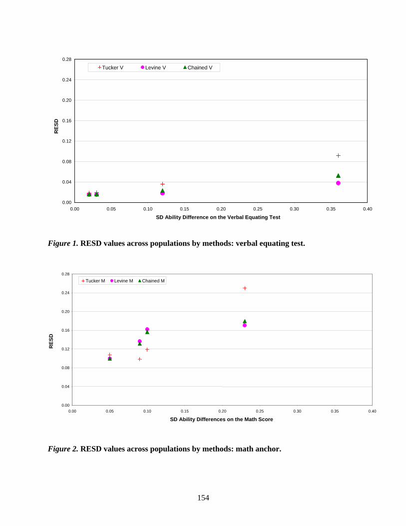
0.00

0.04

0.08

0.12

0.16

0.20

0.24

0.28

0.00 0.05 0.10 0.15 0.20 0.25 0.30 0.35 0.40

SD Ability Difference on the Verbal Equating Test

RES

D

Tucker V Levine V Chained V

Figure 1. RESD values across populations by methods: verbal equating test.

0.00

0.04

0.08

0.12

0.16

0.20

0.24

0.28

0.00 0.05 0.10 0.15 0.20 0.25 0.30 0.35 0.40

SD Ability Differences on the Math Score

RES

D

Tucker M Levine M Chained M

Figure 2. RESD values across populations by methods: math anchor.

154

0.00

0.04

0.08

0.12

0.16

0.20

0.24

0.28

0.00 0.05 0.10 0.15 0.20 0.25 0.30 0.35 0.40

Std Ability Difference on the Composite of Verbal Equating and Math Score

RES

DTucker Comp Levine Comp Chained Comp Tucker Bi

Figure 3. RESD values across populations by methods: COMP anchor.

In addition to RESD, we computed biases, the mean differences between the scores

obtained by the criterion equating and those obtained by each anchor test equating, using the

frequencies for the new form sample. These are presented in Table 7 and plotted in Figures 4-6.

Table 7

Standardized Bias Values Across Population by Methods

Tucker Levine Chained Population Va MT COMP BiV Va MT COMP Va MT COMP Similar 0.02 0.09 0.10 0.03 0.01 0.12 0.11 0.01 0.12 0.11 Close 0.02 0.12 0.12 0.04 0.01 0.15 0.13 0.02 0.15 0.13 Distant 0.04 0.11 0.10 0.04 0.02 0.09 0.09 0.02 0.09 0.09 Far 0.09 0.25 0.15 0.09 0.04 0.17 0.12 0.05 0.18 0.11

Note. BiV = bivariate anchor; Va = verbal anchor; MT = math anchor; COMP = composite

anchor.

155

0.00

0.05

0.10

0.15

0.20

0.25

0.30

0.00 0.05 0.10 0.15 0.20 0.25 0.30 0.35 0.40 0.45

Std Ability Difference on the Verbal Equating Test

Bia

s

Tucker V Levine V Chained V

Figure 4. BIAS values across populations by methods: verbal equating test.

0.00

0.05

0.10

0.15

0.20

0.25

0.30

0.00 0.05 0.10 0.15 0.20 0.25 0.30 0.35 0.40 0.45

Std Ability Difference on the Math Score

Bia

s

Tucker M Levine M Chained M

Figure 5. Bias values across populations by methods: math anchor.

156

0.00

0.05

0.10

0.15

0.20

0.25

0.30

0.00 0.05 0.10 0.15 0.20 0.25 0.30 0.35 0.40 0.45

Std Ability Difference on the Composite of Verbal Equating and Math Score

Bia

s

Tucker Comp Levine Comp Chained Comp Tucker Bi

Figure 6. Bias values across populations by methods: COMP anchor.

The values of both RESD and the standardized bias show that for any level of mean

ability difference the verbal anchor produces the best equating results. In the Similar and Close

samples, the three equating methods produce comparable results when they use the verbal

equating test: Levine is slightly superior to chained, which is slightly superior to Tucker. The

Tucker bivariate anchor is close to these methods. In the Far sample, the separation among the

methods becomes more obvious. Here Levine with the verbal equating test anchor is the most

effective method, whereas the math anchor with Tucker is the least effective method. In the

Distant sample, where the ability difference on the math anchor is the smallest (see Table 1), the

three methods produce comparable results. In the Similar and Close samples, Tucker makes

better use of the math and composite anchors than Levine or chained; whereas in the Far sample,

Levine and chained make better use of the math and the composite anchors than Tucker. Linking

through the bivariate anchor is always better than linking through math or the composite of

verbal and math, which is expected given that the populations were established through selection

on the bivariate surface of verbal and math scores.

The results obtained with the verbal anchor test here are consistent with some results

obtained by Petersen et al. (1982). Tucker does not work as well as Levine with large ability

157

differences (chain works better than Tucker but not as well as Levine), where equating is hard to

achieve. Use of an anchor composed of dissimilar content, such as the math score or the math

score and verbal equating test score composite, does not produce acceptable equating results.

Relative to math, the effectiveness of the composite was less sensitive to ability differences in

this study.

Discussion

This exploratory study built upon research that spans three decades. The massive

Petersen et al. (1982) study is a major empirical investigation of the efficacy of different

equating methods under a variety of conditions. The matched sample work circa 1990 examined

how different equating methods performed across samples that were selected in different ways.

The population invariance studies that built upon Dorans and Holland (2000) have examined

whether different equating methods produce common linking functions for males and females, as

well as across other groups.

What have we found with this integrative study? First, inappropriate anchors did not yield

sound equatings, but they did seem to yield a strong degree of invariance. Appropriate content

(e.g., a verbal anchor for equating verbal tests), produced slightly more subpopulation sensitive

results and equating results consistent with previous findings: solid results with small ability

differences and a divergence of methods with large ability differences. Tucker did not work as

well as Levine and, to a lesser extent, chained under the large ability difference condition.

Tucker did work better, however, with the inappropriate anchors. Tucker with the bivariate

anchor performed as well as Tucker with the verbal equating test in terms of reproducing the

criterion equating, and this combination exhibited more population invariance.

Tucker with any anchor is a poststratification adjustment procedure (von Davier et al.

2004b). It works well when the stratification variable is highly related to the test and uses the

degree of relationship between total test and anchor to make its adjustment. Tucker discounts

inappropriate anchors more than Levine and chained, and, as a consequence, leans more heavily

on the premise that the groups are similar in ability (as they are in the similar and close cases and

less so elsewhere). Tucker is not based on any psychometric model.

Levine, in contrast, is based on psychometrics. It uses bivariate information as well as

reliability information. In this study, we used the Angoff (1971) estimate of reliability, which

assumes that the true scores for the anchor and total test are perfectly correlated. This assumption

158

made eminent sense for the verbal anchor, but not for the math anchor nor for the composite

anchor. It would be interesting to see how Levine worked with different reliability estimates. But

still , the point remains that Levine makes strong classical test theory assumptions that are

inappropriate when anchors measure something different from the score being equated.

Chained ignores bivariate information and makes differences on the total test match those

on the anchor test. This works well with the verbal anchor, but not with the math or composite

anchors.

The results obtained for the bivariate anchor are promising, especially with respect to

population invariance. However, the high correlation that the verbal anchor has with the verbal

test (just under .9) does not allow the math test to add much to the predictability of the verbal

score.

Why were the linkings that used the inappropriate anchors slightly less population

sensitive than those that used the appropriate verbal equating test anchor? All the methods

exhibited acceptable levels of population invariance. Population invariance is a prerequisite for

equating. Lack of population invariance can be taken as evidence that a linking is not an

equating. The existence of invariance, however, does not necessarily mean that the score

interchangeability sought by equating has been achieved. If it did, we could just use the identity

equating, or any other data-free score conversion for all tests because they are, by definition,

invariant. Thus, population invariance cannot be used as the sole criterion for assessing the

quality of equating.

In addition to further empirical work with test data that are not so well behaved, we need

to consider analytical explanations for some of these findings, particularly those related to

population invariance. More extensive research is needed before some of these results can be

viewed as definitive.

159

A Discussion of Population Invariance of Equating

Nancy S. Petersen

ACT, Inc., Iowa City, IA

161

Abstract

This paper discusses the five studies included in this report. Each paper addresses the same issue,

population invariance of equating, they all used data from major standardized testing programs,

and they all used essentially the same statistics to evaluate their results, namely, the root mean

squared difference (RMSD) and root expected mean squared difference (REMSD, Dorans &

Holland, 2000).

162

Acknowledgments

The author is grateful to Deborah Harris for comments on a previous draft of this paper.

163

Introduction

This paper discusses the five studies included in this report. Each paper addresses the

same issue, population invariance of equating. They all used data from major standardized

testing programs, and they all used essentially the same statistics to evaluate their results,

namely, the root mean squared difference (RMSD) and root expected mean squared difference

(REMSD; Dorans & Holland, 2000).

The major premise underlying all of these papers is that population invariance is a

prerequisite for equating, and, lack of population invariance can be taken as evidence that a

linking is not an equating.

First, a brief summary of the study design and results for each paper.

The paper by von Davier and Wilson (2006, this volume, pp. 1–28) investigated

population invariance for gender groups for the AP Calculus AB exam. They used an internal

anchor test data collection design to equate a multiple-choice (MC) test and a test composed of

both MC and free response questions. Item response theory (IRT), Tucker, and chained linear

equating procedures were used. Overall, the two administration groups did not differ much in

ability, but the gender groups had large differences in ability. In general, they found that all

equating methods produced acceptable and comparable results for both tests for equatings based

on men, women, or total administration groups.

The paper by Liu and Holland (2006, this volume, pp. 29–58) used LSAT data from a

single administration to investigate population invariance for highly reliable parallel tests, for

less reliable parallel tests, and for nonparallel tests. They used subgroups based on gender,

race/ethnicity, geographic location, application to law school status, and admission to law school

status. As expected, they found that construct similarity between the two tests to be equated had

much more effect on the population sensitivity of results than did differences in reliability.

The paper by Yang and Gao (2006, this volume, pp. 59-98) looked at population

invariance for gender groups for forms of the College-Level Entrance Placement® (CLEP®)

College Algebra exam. This was an equivalent groups design. In general, they found that

equating results based on men, women, or total group were comparable overall and at the cut-

score.

The paper by Yi, Harris, and Gao (2006, this volume, pp. 99–130) also used an

equivalent groups design with a science achievement test. Unlike the other researchers, though,

164

they looked at population invariance for subgroups that differed in ability. They created three

sets of subgroups of dissimilar ability: (a) based on the average of four test scores that included

the science test under study, (b) based on students’ average GPA in all science courses taken, and

(c) based on whether students had taken physics. I would expect differences in ability for the

latter two sets of subgroups to be more closely related to performance on the science test and the

data in Table 1 of their paper supports this. Raw score differences for the composite subgroups

were approximately 1 point, those for the GPA subgroups were approximately 4 points, and

score differences for the physics subgroups were approximately 5 points. When the ability

differences among the groups of interest were related to the construct being measured, they

found the equating functions to be more population sensitive.

The paper by Dorans, Liu, and Hammond (2006, this volume, pp. 131–160) looked at the

effect of anchor test, ability group differences, and equating method on population invariance for

gender groups. Results of this study reconfirm results of several earlier studies. The Tucker

equating method does not work well when there are large ability differences between the groups.

Also, use of an anchor composed of dissimilar content to the tests to be equated does not produce

acceptable equating results.

In summary, these five studies found little sensitivity of equating results for subgroups

formed on the basis of characteristics such as gender, race/ethnicity, and geographic location.

They found that the use of anchor tests that were not miniatures of the tests to be equated did not

yield sound equatings. They also found that the Tucker equating method did not work well when

there were large differences in group ability. They found that construct similarity between the

two tests to be equated had much more effect on the population sensitivity of results than did

differences in test reliability. Finally, they found some sensitivity of equating results for

subgroups that were selected on variables related to the construct being measured.

So, to reiterate: all these papers are based on the premise that population invariance is a

prerequisite for equating.

Just when is a linking an equating? Most practitioners would agree that there are five

requirements for a linking between scores on two tests to be considered an equating (Dorans &

Holland, 2000; Lord, 1980; Petersen, Kolen, & Hoover, 1989):

165

1. Same construct—the two tests must both be measures of the same characteristic (latent

trait, ability, or skill).

2. Equal reliability—scores on the two tests are equally reliable.

3. Symmetry—the transformation is invertible.

4. Equity—it does not matter to examinees which test they take.

5. Population invariance—the transformation is the same regardless of the group from

which it is derived.

In reality, equating is used to fine-tune the test-construction process. We equate scores on

tests because of our inability to construct multiple forms of a test that are strictly parallel. Thus,

the same construct and equal reliability constraints simply imply that the two tests to be equated

should be built to the same blueprint, that is, to the same content and statistical specifications.

The study by Liu and Holland (2006, this volume, pp. 29–58) illustrates the importance of

construct similarity in the tests to be equated.

The population invariance and symmetry conditions follow from the purpose of equating:

to produce an effective equivalence between scores. If scores on two tests are equivalent, then

there is a one-to-one correspondence between the two sets of scores. This implies that the

conversion is unique, that is, that the transformation must be the same regardless of the group

from which it is derived. And, it further requires that the transformation be invertible. That is, if

score yo on test Y is equated to score xo on test X, then xo must equate to yo. Thus, regression

methods cannot be used for equating.

The same ability and population invariance conditions go hand-in-hand, as do the same

ability and equity conditions. If the two tests were measures of different abilities, then the

conversions would certainly differ for different groups (see Liu & Holland, 2006, this volume,

pp. 29–58). And, if the two tests measure different skills, then examinees will prefer the test on

which they will score higher.

But I have a mixed view of population invariance as a prerequisite for equating. As a

practitioner, I believe all equatings are population dependent. At the same time, when I am

working on a testing program that reports scores from multiple test forms, I must somehow link

or equate scores across those many test forms.

166

When Paul Holland and Henry Braun finished their chapter in the book, Test Equating,

(Braun & Holland, 1982), Holland concluded that all equatings are population dependent to

some degree. Also, he convinced me to always treat equating as population dependent. Data

from some of my own research reinforced this belief, as does data from some of the studies

included in this report.

If the tests to be equated are constructed to be parallel in content and difficulty; we have a

strong data collection design, for example, equivalent groups or an anchor test design in which

the anchor test is a miniature of the total tests; and we use equating methods appropriate for the

data collection design, for example, only Tucker if groups are similar in ability then I would

expect equating results to be population invariant for subgroups selected on something unrelated

to the construct being measured.

That is, just as was found in these studies, I would expect, in general, to find comparable

equating results for groups selected on characteristics such as gender, race/ethnicity, and

geographic region.

However, if the selection variable for constructing the subgroups is related to the

construct being measured, I would expect the equating results to exhibit population dependence.

This is supported by the findings for the science achievement test reported on by Yi, Harris, and

Gao (2006, this volume, pp. 99–130). It’s also supported by findings from earlier studies. For

example, Cook and Petersen (1987) found that when relatively parallel forms of a biology

achievement test were equated using groups of students who took the tests at different times of

the year (May and December), they got very disparate equating results. Upon investigation, they

found similar equating results for groups who took the tests at the same time of the year

(May/May or December/December). Upon closer examination of the administration groups, they

came to realize that students taking the test in May were primarily sophomores completing a

course in biology, whereas students taking the test in December were primarily seniors who had

not taken biology since their sophomore year. They concluded that the disparate equating results

were obtained because students taking the test at the different times of the year differed in

relative recency of their coursework. This difference in recency of training interacted with test

content. Thus, the biology test measured different constructs, depending on the sample of

examinees to whom the test was administered. Similar results have also been found for tests of

167

English as a foreign language when subgroups are selected based on type of first language

learned.

Petersen et al. (1989) provided an extreme example of the population dependency of

equating. Suppose that two test forms are essentially alike except that one is more difficult.

Further suppose that the equating is carried out using groups of examinees that guess at random.

In this case, the difference in difficulty between the two test forms would not be evident, and the

equating transformation derived would be essentially the identify function. However, if a more

competent group of examinees were used for the equating, the difference in difficulty would be

evident, and the scores on the harder form would be adjusted accordingly in relation to the scores

on the easier form. Thus, in practice, it is best to use a heterogeneous group for equating.

So, I’ve come to believe that all equatings are, first and foremost, population dependent.

Even when tests are built to the same precise content and statistical specifications, it is possible

that the characteristics measured by the test might differ somewhat from one group of individuals

to another. Thus, in practice, it is critical that careful thought be given to the selection of the

group to be used routinely for equating. In practice, it’s very important that all operational testing

programs conduct population invariance studies to determine if there are any major subgroups of

interest for which the equating results may not be comparable, given the various data collection

designs that could be used.

Given today’s social and political climate, I would recommend that all testing programs

with high-stakes outcomes conduct population invariance equating studies for gender and major

racial/ethnic subgroups, especially since the results are likely to be comparable across these

subgroups. Testing programs also need to conduct studies for major subgroups that could differ

in ways related to the ability being measured and/or that comprise a varying proportion of the

testing population at different administrations. For example, does it matter if repeaters are

included in the equating sample? How about using all test takers, including international

students, versus only domestic students? For foreign language tests, does it matter if native

speakers or first-year students are included in the equating sample?

If the conversions for various subgroups of interest are not comparable or population

invariant, then the psychometric implication is that different conversions should be used for

different groups. However, in practice, testing programs cannot use different linkings for

different groups. In today’s social and political climate, it would be very difficult for a testing

168

program to justify assigning different reported scores to two candidates from different groups

who have the same raw score on the test. So, if the results of population invariance studies show

indications of population sensitivity, then great care needs to be taken in selecting a data

collection design and a subpopulation (of the total testing population) for use for all item and test

analyses and for score equating. And, the subpopulation for which score comparability is

expected to hold should be specified in the programs’ technical manual. Careful specification of

the analysis population used for a test will improve score equity and improve scale stability

across test administrations and test forms.

169

A Discussion of Population Invariance

Robert L. Brennan

University of Iowa, Iowa City, IA

171

Acknowledgments

The author is grateful to Michael J. Kolen and Neil J. Dorans for comments on a previous draft

of this paper.

172

The volume discussed here consists of five papers that are linked in the sense that they all

treat population invariance:

• von Davier and Wilson (2006, pp. 1–28) considered IRT equating for the AP exams;

• Liu and Holland (2006, pp. 29–58) considered parallel-linear linking for the LSAT;

• Yang and Gao (2006, pp. 59–98) considered linking for CLEP exams that consist of

overlapping groups of testlets;

• Yi, Harris, and Gao (2006, pp. 99–130) considered equating for a science

achievement test; and

• Dorans, Liu, and Hammond (2006, pp. 131–160) considered the role of an anchor test

in achieving population invariance.

The discussion here of population invariance is a somewhat broader treatment of the

subject than simply a discussion of these five papers. In particular, occasional reference is made

to publications other than those in this report.

Dorans et al. (2006, this volume, p. 134) stated, “Tests are equatable to the extent that the

same equating function is obtained across significant subpopulations ….” This is an accurate

statement provided it is understood in the sense that population invariance is a necessary but not

sufficient condition for equating. If population invariance is not satisfied, then the resulting

relationship can be no stronger than a linking. Of course, population invariance is a matter of

degree. Here, to avoid needlessly complicated statements, I sometimes use the term linking to

include equating. In particular contexts, typically it is not too difficult to persuade reasonable

persons to agree about whether the term equating or linking applies.

As Kolen (2004) pointed out, the literature on population invariance and linking extends

back at least to Flanagan’s (1951) “Units, Scores, and Norms” chapter in the first edition of

Educational Measurement. However, it wasn’t until Mislevy (1992) and Linn (1993) published

their linking taxonomies in the early 1990s that linking became highly visible to the

measurement community. Then, later in that decade, the Uncommon Measures report (Feuer,

Holland, Green, Bertenthal, & Hemphill, 1999) from the National Research Council addressed

linking directly, and the Embedding Questions report (Koretz, Berenthal, & Green, 1999)

addressed the topic as well, although less directly. Since then, there has been a substantial

173

increase in the literature on linking. For example, two special issues of journals were devoted to

linking in 2004: Journal of Educational Measurement, 41(1), edited by Dorans (2004a) and

Applied Psychological Measurement, 28(4), edited by Pommerich and Dorans (2004). Kolen and

Brennan (2004) also provided an entire chapter devoted to linking. The papers in this report are

an important addition to the literature, especially because they provide real-data examples that

illustrate important issues in linking.

For the tests considered in these papers, the results reported provide support for at least

the following tentative conclusions:

• population invariance tends to be satisfied reasonably well for carefully constructed

alternate forms of a test with equal reliability (Liu & Holland, 2006, this volume, pp.

29–58; Yang & Gao, 2006, this volume, pp. 59–98),

• linking functions tend to be more similar for gender groups than for ethnic groups

(Liu & Holland, 2006, this volume, pp. 29–58; Yang & Gao, 2006, this volume, pp.

59–98),

• linking functions tend to be more similar for tests that differ in reliability than for

tests that measure different constructs (Liu & Holland, 2006, this volume, pp. 29–58),

• often (but not always) population invariance results are quite consistent across types

of linking methods (von Davier & Wilson, 2006 this volume, pp. 1–28; Yi et al.,

2006, this volume, pp. 99–130), and

• satisfying the assumption of population invariance does not guarantee that a linking can

be considered an equating (Dorans et al., 2006, this volume, pp. 131–160).

These conclusions are reasonably consistent with other literature, although, of course, not

all of them will necessarily hold for other tests or other contexts. Also, it is important to note that

many of these conclusions are based largely on the Dorans and Holland (2000) root mean

squared difference (RMSD) and root expected mean squared difference (REMSD) statistics (or

extensions of them), which are considered in more detail below.

RMSD and REMSD Statistics

Dorans and Holland (2000) introduced the RMSD and REMSD statistics to quantify the

extent to which linking functions are population invariant. Strictly speaking, their paper dealt

174

only with linear linking for the single group design and neglected counterbalancing (if any),

although many results also apply to the random groups design. Also, strictly speaking, their

paper considered observed score equating only. Subsequent extensions of the RMSD and

REMSD statistics are discussed by von Davier, Holland, and Thayer (2003, 2004a); von Davier

and Wilson (2006, this volume, pp. 1–28); and Yin, Brennan, and Kolen (2004). See also Kolen

and Brennan (2004, chapter 10).

The basic RMSD equation for a linking of scores on X to scores onY is.1

( ) ( )2

RMSD( ) jj P Pj

YP

w e x e xx

σ

⎡ ⎤−⎣=∑ ⎦ , (1)

where e denotes a linking function, P denotes the total population, {Pj}denotes a partition of P

into mutually exclusive and exhaustive subpopulations (P1, P2, …, Pk ), and ( )

is the weight given to subpopulation Pj. A single number summarizing

k jw 0 1jw< <

( )RMSD x is obtained by

averaging over the distribution of X in P before taking the square root:

( ) ( )2

REMSD jj P P Pj

YP

w E e X e X

σ

⎡ ⎤−⎣=∑ ⎦ , (2)

Where E is the expectation operator. Note that (2) is a doubly weighted statistic. The weights

are weights for each of the subpopulations, and taking the expectation over P involves weighting

the scores on

jw

X in some sense (discussed later).

When it is assumed that the slope of the linking functions is the same for all

subpopulations, RMSD( )x is a constant for all values of x , and the resulting value of REMSD for

such parallel-linear (pl) linking functions is

2

REMSD j jXP XPYP YPjpl

j YP X P

wμ μμ μ

σ σ

⎡ ⎤−⎛ ⎞ ⎛−= −⎢⎜ ⎟ ⎜⎜ ⎟ ⎜⎢ ⎥⎝ ⎠ ⎝⎣ ⎦∑

⎞.⎥⎟⎟

⎠ (3)

If, in addition, there are only two subpopulations ( 2k = )

1 2 1 22 1 2REMSD YP YP XP XP

plYP X P

w wμ μ μ μ

σ σ⎛ ⎞ ⎛− −

= −⎜ ⎟ ⎜⎜ ⎟ ⎜⎝ ⎠ ⎝

⎞.⎟⎟

⎠ (4)

175

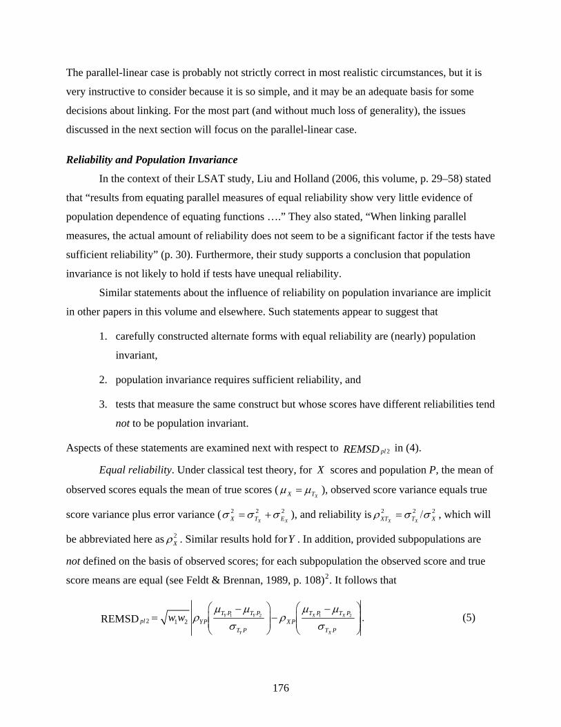
The parallel-linear case is probably not strictly correct in most realistic circumstances, but it is

very instructive to consider because it is so simple, and it may be an adequate basis for some

decisions about linking. For the most part (and without much loss of generality), the issues

discussed in the next section will focus on the parallel-linear case.

Reliability and Population Invariance

In the context of their LSAT study, Liu and Holland (2006, this volume, p. 29–58) stated

that “results from equating parallel measures of equal reliability show very little evidence of

population dependence of equating functions ….” They also stated, “When linking parallel

measures, the actual amount of reliability does not seem to be a significant factor if the tests have

sufficient reliability” (p. 30). Furthermore, their study supports a conclusion that population

invariance is not likely to hold if tests have unequal reliability.

Similar statements about the influence of reliability on population invariance are implicit

in other papers in this volume and elsewhere. Such statements appear to suggest that

1. carefully constructed alternate forms with equal reliability are (nearly) population

invariant,

2. population invariance requires sufficient reliability, and

3. tests that measure the same construct but whose scores have different reliabilities tend

not to be population invariant.

Aspects of these statements are examined next with respect to 2plREMSD in (4).

Equal reliability. Under classical test theory, for X scores and population P, the mean of

observed scores equals the mean of true scores (XX Tμ μ= ), observed score variance equals true

score variance plus error variance ( 2 2XX T E

2X

σ σ σ= + ), and reliability is 2 2X XXT T X

2ρ σ σ= / , which will

be abbreviated here as 2Xρ . Similar results hold for . In addition, provided subpopulations are

not defined on the basis of observed scores; for each subpopulation the observed score and true

score means are equal (see Feldt & Brennan, 1989, p. 108)

Y

2. It follows that

1 2 1 22 1 2REMSD Y Y X X

Y X

T P T P T P T Ppl YP X P

T P T P

w wμ μ μ μ

ρ ρσ σ

⎛ ⎞ ⎛− −= −⎜ ⎟ ⎜⎜ ⎟ ⎜

⎝ ⎠ ⎝

⎞.⎟⎟

⎠ (5)

176

Note that YPρ and X Pρ are the square roots of the reliabilities in P. Clearly, if the reliabilities of

X and Y are equal in P, then X P YP Pρ ρ ρ= = , and

1 22 1 2REMSD Y Y X 1 X 2

Y X

T P T P T P T Ppl P

T P T P

w wμ μ μ μ

ρσ σ

⎛ ⎞ ⎛− −= −⎜ ⎟ ⎜⎜ ⎟ ⎜

⎝ ⎠ ⎝

⎞.⎟⎟

⎠ (6)

The derivation of (6) makes no assumption about the relationship between X andY . However,

this equation does reveal that, under the equal reliability condition, a reduction in reliability gets

one closer to population invariance.3 This is not as paradoxical as it may seem initially. For

example, if data are generated randomly for two tests, and examinees are randomly assigned to

subpopulations, then reliability will be 0 and population invariance will be attained. In short, (6)

does not support the sufficient reliability requirement in Statement 2.

There is another implication of (6) that may seem counterintuitive: namely, population

invariance is not assured when reliability is 1. Again, this is not as paradoxical as it may seem.

One explanation is that even if we have true scores for examinees, linkings based on observed

score procedures are not necessarily population invariant. This is a subtle issue because we need

to distinguish between the nature of the examinee scores as well as the type of procedure used to

generate the linking. In a related vein, in his review of the history of population invariance,

Kolen (2004) stated

Based on the equity property and using a unidimensional IRT framework, Lord and

Wingersky (1984, p. 456) indicated that IRT observed score equating relationships hold

“precisely only for that total group [used to define the equating relationship] and not for

other groups or subgroups.” Lord and Wingersky also indicated that under an IRT model,

true score equating is invariant for subpopulations within a population. However, they

pointed out that true scores are not known and there is no theoretical reason to apply the

true score relationship to observed scores, even though this is often done in practice. (p. 6)

Tau equivalent and classically parallel. The preceding discussion of the equal reliability

condition is an incomplete analysis of Statement 1 in that the discussion never formally

incorporates the alternate forms part of the statement. There are numerous definitions of alternate

forms, each of which can be viewed as a different answer to the question of what constitutes a

replication of the measurement procedure. (See Brennan, 2001.) If scores on X and Y are

177

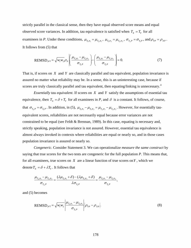
strictly parallel in the classical sense, then they have equal observed score means and equal

observed score variances. In addition, tau equivalence is satisfied when for all

examinees in P. Under these conditions,

XT T= Y

1 1Y XT TP Pμ μ= , 2 2Y XT TP Pμ μ= ,

XT P T PYσ σ= , and YP X Pρ ρ= .

It follows from (5) that

1 2 1 22 1 2 0REMSD Y Y Y Y

Y Y

T T T TP P P Ppl P

T P T P

w wμ μ μ μ

ρσ σ

⎛ ⎞ ⎛ ⎞− −= −⎜ ⎟ ⎜⎜ ⎟ ⎜

⎝ ⎠ ⎝ ⎠= .⎟⎟ (7)

That is, if scores on X and Y are classically parallel and tau equivalent, population invariance is

assured no matter what reliability may be. In a sense, this is an uninteresting case, because if

scores are truly classically parallel and tau equivalent, then equating/linking is unnecessary.4

Essentially tau equivalent. If scores on X and Y satisfy the assumptions of essential tau

equivalence, then XT YTδ= + for all examinees in P, and δ is a constant. It follows, of course,

that XT P T PY

σ σ= . In addition, in (5), 1 2 2Y Y XT T T1XTμ −P P P Pμ μ μ= − . However, for essentially tau-

equivalent scores, reliabilities are not necessarily equal because error variances are not

constrained to be equal (see Feldt & Brennan, 1989). In this case, equating is necessary and,

strictly speaking, population invariance is not assured. However, essential tau equivalence is

almost always invoked in contexts where reliabilities are equal or nearly so, and in those cases

population invariance is assured or nearly so.

Congeneric. Consider Statement 3. We can operationalize measure the same construct by

saying that true scores for the two tests are congeneric for the full population P. This means that,

for all examinees, true scores on X are a linear function of true scores onY , which we

denote XT YTδ λ= + . It follows that

1 2 1 2 1( ) ( )

X X Y Y Y Y

X Y

T T T T T TP P P P P P

T P T P T P

2

Y

μ μ λμ δ λμ δ μ μσ λσ− + − + −

= =σ

,

and (5) becomes

1 22 1 2REMSD Y Y

Y

T TP Ppl YP X P

T P

w wμ μ

ρ ρσ−

= − . (8)

178

As discussed by Feldt and Brennan (1989), reliabilities can be unequal for congeneric tests,

because neither true score variances nor error variances are constrained to be equal. Clearly, all

other things being unchanged, the larger the discrepancy between reliabilities, the larger the

value of , in accordance with Statement 3. Note, however, that it is the absolute value

of the difference in reliabilities that matters, not their individual magnitudes, which contradicts

the spirit of Statement 2.

2REMSD pl

5

Upper limit arguments. Dorans and Holland (2000) provided the following upper limit

for : 2REMSD pl

2 2(1 )REMSD pl XYPρ≤ − , (9)

where XYρ P is the product-moment correlation in the full population P. They were careful to

state, “For real distributions of test scores it is likely to be too high, but at this stage of our

understanding it is the only upper bound that we have” (p. 292). Still, it is clear that this upper

limit (right side of ) gets smaller as the observed score correlation, 2REMSD pl XYρ P , gets larger,

and an observed score correlation tends to get larger as reliability tends to get larger. This may

appear to support the conclusion that high reliability is a necessary requirement for population

invariance (i.e., small value for ). Actually, however, this conclusion is not

necessarily true. An upper limit for a particular statistic merely states that the statistic cannot be

larger than the upper limit; the upper limit does not dictate a monotonic relationship between the

statistic ( , here) and one of its components (

2REMSD pl

2REMSD pl XYPρ , here).

Consider, for example, given by (8) for the parallel-linear case with the

congeneric model and two groups. Suppose that the weights are equal, and the standardized

difference in means is 1. In this case, true scores are perfectly correlated (

2REMSD pl

1X YT T Pρ = ), and Table 1

provides and upper-limit results for five selected pairs of reliabilities.2REMSD pl6 The results in

Table 1 are ordered from high to low values, but the corresponding upper limits are

not consistently ordered in the reverse direction. Note, as well, that the observed correlation in

any row is actually the geometric mean of the reliabilities in that row. Clearly, higher reliability

(in the geometric mean sense) always leads to a smaller value for the upper limit, but higher

reliability does not always translate into a lower value for .

2REMSD pl

2REMSD pl

179

Table 1

An Example of the Influence of Reliabilities on REMSDpl2 and the Dorans and Holland

(2000) Upper Limit When the True Score Correlation Is 1 2XPρ 2

YPρ XYPρ REMSDpl2 2(1 )XYPρ−

.7 .9 .79373 .056 .642

.7 .8 .74833 .029 .709

.8 .9 .84853 .027 .550

.8 .8 .80000 .000 .632

.7 .7 .70000 .000 .775

The importance of reliability. Admittedly, the preceding discussion of reliability and

population invariance is restrictive in several ways. For example, results have been considered

for , only. Still, it seems eminently clear that high reliability is not a necessary

condition for population invariance, and there is no compelling empirical evidence to the contrary

in the papers in this report. This definitely does not mean, however, that reliability is unimportant

for a useful and meaningful linking. Even if population invariance is satisfied, if scores are highly

unreliable, any resulting linking is little more than a statistical manipulation of noise.

2REMSD pl

So, in summary, I conclude that (a) tests that differ in reliability are likely to exhibit

population sensitivity, (b) increasing reliability does not necessarily enhance the likelihood of

population invariance, and (c) high reliability is usually necessary for a useful linking. It may

appear that (c) contradicts (b), but that is not the case. Rather, the message here is that although

population invariance is a useful criterion, it is only one criterion for linking, and satisfying

population invariance does not guarantee an adequate linking. This message is consistent with

statements made by Dorans et al. (2006, this volume, pp. 131–160).

Weights

Both the RMSD and REMSD statistics involve weights for each of the

subpopulations. In addition, the REMSD statistic involves taking the expectation over P, which

means that the scores on

jw

X are weighted.

The two seemingly obvious choices for the jw are equal weights ( ) and weights

proportional to sample sizes. In fact, various papers in this report provide results for both sets of

weights. Presumably, one would choose equal weights if the subpopulations are equally important

1jw = /k

180

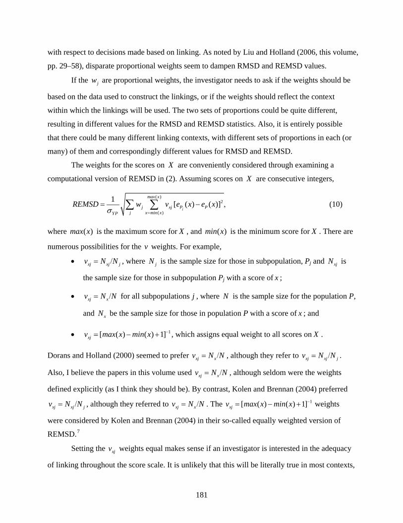
with respect to decisions made based on linking. As noted by Liu and Holland (2006, this volume,

pp. 29–58), disparate proportional weights seem to dampen RMSD and REMSD values.

If the are proportional weights, the investigator needs to ask if the weights should be

based on the data used to construct the linkings, or if the weights should reflect the context

within which the linkings will be used. The two sets of proportions could be quite different,

resulting in different values for the RMSD and REMSD statistics. Also, it is entirely possible

that there could be many different linking contexts, with different sets of proportions in each (or

many) of them and correspondingly different values for RMSD and REMSD.

jw

The weights for the scores on X are conveniently considered through examining a

computational version of REMSD in (2). Assuming scores on X are consecutive integers,

( )2

( )

1 [ ( ) ( )]j

max x

j xj P Pj x min xYP

REMSD w v e x e xσ =

= ∑ ∑ − , (10)

where is the maximum score for( )max x X , and is the minimum score for( )min x X . There are

numerous possibilities for the v weights. For example,

• xj xjv N N= / j , where is the sample size for those in subpopulation, Pj and jN xjN is

the sample size for those in subpopulation Pj with a score of x ;

• for all subpopulationsxj xv N N= / j , where is the sample size for the population P,

and

N

xN be the sample size for those in population P with a score of x ; and

• 1[ ( ) ( ) 1]xjv max x min x −= − + , which assigns equal weight to all scores on X .

Dorans and Holland (2000) seemed to prefer xj xv N N= / , although they refer to xj xjv N N= / j .

Also, I believe the papers in this volume used xj xv N N= / , although seldom were the weights

defined explicitly (as I think they should be). By contrast, Kolen and Brennan (2004) preferred

xj xjv N N= / j , although they referred to xj xv N N= / . The weights

were considered by Kolen and Brennan (2004) in their so-called equally weighted version of

REMSD.

1[ ( ) ( ) 1]xjv max x min x −= − +

7

Setting the xjv weights equal makes sense if an investigator is interested in the adequacy

of linking throughout the score scale. It is unlikely that this will be literally true in most contexts,

181

but often it is approximately true and/or equal weights may be a better reflection of the

investigator’s interest than data-based weights.

The data-based weights ( xj xjv N N= / j and xj xv N N= / ) could be based on the data used to

construct the linking, or the weights could reflect the context within which the linkings will be

used. That is, choosing data-based weights for X scores involves the same types of judgments

involved in choosing data-based weights for the jw .

Almost all of the papers in this volume provide plots of RMSD( )x , which are quite

informative. See (1). In making judgments about the jw and X -score weights, it is helpful to

recall that such plots involve the weights but do not involve the jw X -score weights. So, the

gestalt provided by a plot of RMSD( )x is one of equally-weighted X scores.

In addition, most of the papers provide plots of subgroup differences, or subgroup minus

total group differences, for the various X scores. These plots are particularly helpful, I believe. I

would suggest that they be provided routinely when population invariance is under

consideration.

Difference That Matters

In evaluating any statistic, it is natural to ask whether the magnitude is large enough to be

important in some sense. In equating contexts, for many years ETS has answered this question in

part using the notion of a difference that matters (DTM; see, for example, Dorans & Feigenbaum,

1994), which is half of a reported score unit. Given this history, it is natural that a DTM be used

as a benchmark for the RMSD and REMSD statistics. Since these two statistics are standardized

by dividing by YPσ (usually), the DTM is often standardized by dividing by the same quantity,

which I denote as SDTM (see also von Davier & Wilson, 2006, this volume, pp. 1–28).

Roughly speaking, the DTM/SDTM logic applied to linking is that rounding to reported

scores introduces systematic errors, and a subgroup linking that is within half a reported score

unit of the combined group linking (at a given raw score point) is ignorable. This convention

needs to be understood, however, as a convenient benchmark, not a dogmatic rule, especially

when it is applied to an overall statistic such as REMSD. For example, even when REMSD is

less than SDTM, it is likely that some of the component RMSD values will be greater than

182

SDTM, and some smaller, depending on the value of X . In such circumstances, simply reporting

that REMSD is less than SDTM may be quite misleading.

RMSD and REMSD were originally proposed by Dorans and Holland (2000) in the

context of observed score linking procedures and simple designs. von Davier and Wilson (2006,

this volume, pp. 1–28) extended these statistics to IRT true score equating. Doing so involves a

conceptual complexity. If the assumptions of IRT hold, then IRT true score equating is invariant

over all subpopulations, which seems to make the task of examining invariance irrelevant.

However, in general, the population invariance of IRT true score equating does not hold when

equating functions are used with observed scores. (Recall the previous citation from Kolen,

2004.) In this sense, in theory, IRT true score equating is necessarily an equating, but in practice

it is not guaranteed to be an equating.

von Davier et al. (2004a) and von Davier and Wilson (2006, this volume, pp. 1–28)

discussed extensions of RMSD and REMSD to more complicated designs, such as the NEAT

design that involves more than one population (called the common-item nonequivalent group

design, CINEG, by Kolen & Brennan, 2004). For such designs, specifying and estimating the

standardization term is considerably more complicated than it is for simple designs. Furthermore,

it may be better to drop the standardization term if the reporting metric has an established

meaning (von Davier et al., 2004a, p. 23), or if RMSD or REMSD statistics are compared that

have different standardization terms.8 Note that Dorans et al. (2006, this volume, pp. 131-160)

provided results for both standardized and unstandardized REMSD statistics.

Rounded Equivalents

Most applications of the RMSD or REMSD statistics are based on unrounded

equivalents. There are exceptions, however. For example, Yi et. al. (2006, this volume, pp. 99–

130) used rounded equivalents, Yang and Gao (2006, this volume, pp. 59–98) used transformed

scores (0/1) that are essentially rounded, and Kolen and Brennan (2004) gave an example using

both rounded and unrounded equivalents. The DTM, in the sense of half a reported score unit,

applies to unrounded equivalents only. I suggest that rounded equivalents have not received as

much attention as they deserve, given the obvious fact that decisions about examinees are almost

always based on rounded equivalents.

183

Other Statistics for Assessing Linking Adequacy

As useful as the RMSD and REMSD statistics can be, they are not the only possibilities

for quantifying population invariance. For example, in the paper in which they introduced these

statistics, Dorans and Holland (2000) provided formulas that focus on the maximum difference

for any subpopulation, along with its expectation in P. Also, Kolen and Brennan (2004, p. 444)

suggested several other statistics for quantifying population invariance, including the mean

absolute difference (MAD) for pairs of subgroups. MAD is simply the weighted average of the

differences between equivalents for pairs of subgroups. If there are only two subgroups,

j and j′ , a computational formula is

'MAD ( ) ( )j jx P P

xe x e xν= −∑ ,

where xν is the relative weight for score x .9 The magnitude of MAD could be evaluated relative

to the unstandardized DTM.

As an example, Kolen and Brennan (2004) discussed linking the Iowa Tests of

Educational Development (ITED) Analysis of Science Materials to the ACT Assessment Science

Reasoning Test.10 For this hypothetical example and the parallel-linear method, when subgroups

are males and females, Y , andITEDscience= X ACTscience= ,

• , with101REMSD = . 12SDTM = . , suggesting that population invariance is satisfied,

and

• , with860MAD = . 5DTM = . , suggesting that population invariance is not satisfied.

Apparently, for this example, choice of a statistic (REMSD or MAD) and the standard for

evaluating it (SDTM or DTM, respectively) makes a difference.11

Kolen and Brennan (2004, pp. 463–465) also suggested considering other statistics when

a linking is being studied. These statistics, discussed next, tend to quantify more about the

strength of a linking than population invariance per se.

184

Correlations With Other Tests

A seemingly sensible benchmark for evaluating the reasonableness of a linking of two

tests is to compare it to some other linking that enjoys the status of being sensible or suffers from

the criticism of being questionable or even ridiculous. This basic idea can be operationalized

using correlation coefficients, as suggested by Dorans and Holland (2000), among others.

To continue the ITED/ACT example, columns 2–4 in the top row of Table 2 provide the

correlations between the ITED and ACT science tests for males, females, and the combined

group. Columns 2–4 of the subsequent rows provide correlations between the ACT science test

and the other ACT tests in English, mathematics, and reading. For each of the three groups

(males, females, and combined), without exception, the correlations between ACT science test

and the other ACT tests are all larger than the correlation between the ACT and ITED science

tests. Assuming that reasonable persons would not use scores for the various ACT tests

interchangeably, such persons should be even less inclined to use the ITED and ACT science test

scores interchangeably. Also, the fact that the ITED/ACT science correlations for males and

females are different provides a suggestion of population sensitivity, although admittedly not as

direct evidence as other statistics discussed previously or next.

Table 2

Relationships Between ACT Science Test and Other Tests

Observed correlations RMSELsa for linear linkingb Test Combined Male Female Combined Male Female

ITED science .672 .660 .689 3.416 3.631 3.157

ACT English .709 .727 .732 3.219 3.253 2.931

ACT math .697 .676 .705 3.286 3.544 3.075

ACT reading .736 .750 .741 3.063 3.110 2.882

Note. From Test Equating: Methods and Practices (2nd ed.) by M. J. Kolen and R. L. Brennan,

2004, New York: Springer-Verlag. Copyright 2004 by Springer-Verlag. Adapted with permission.

a RMSEL = root mean squared error for linking. b Linking to scale of ACT science test.

185

Root Mean Squared Error for Linking

Correlations tell us something about how similar scores are for a pair of variables. We

might also want to quantify the extent to which score equivalents based on a particular linking

method reproduce the Y scores actually observed. To do so, Kolen and Brennan (2004, p. 464)

defined the root mean squared error for linking (RMSEL) as

[ ]2RMSEL ( )Y e XE= −P P . (11)

For the linear method ( ), it can be shown that l

2(1 )l YP XYPRMSEL σ ρ= − . (12)

These RMSEL statistics are expressed here in terms of the combined group, P; corresponding

equations can be defined for any subgroup. For the combined group, RMSEL for the linear and

parallel linear methods are the same, although this is not necessarily true for subgroups.

An example. For the ITED/ACT example, the right-hand part of Table 2 provides

REMSL values for the linear method. One might ask whether or not these values for science are

large or small. As shown by Kolen and Brennan (2004, p. 532), one benchmark is 2SEM ,

where is the standard error of measurement. For the ACT Science Reasoning exam, the

is approximately 2 scale score points,

SEM

SEM 12 which gives a benchmark value of 2 2 2 828= . .

The ITED/ACT RMSEL science values are clearly larger than this benchmark, especially for

males. It follows that there is more error in linking ITED Analysis of Science Materials scores to

ACT Science Reasoning scores than there is in using scores from one form of ACT Science

Reasoning as a proxy for scores on another form of the same test. Note also that these results

provide evidence of population sensitivity, since the ITED/ACT science RMSEL values for

males and females are quite different.

Importance of high correlations. It is evident from (12) that lRMSEL gets smaller as

XYPρ gets larger. Since reducing errors is a central goal of good measurement, it follows that

large values for XYPρ are desirable. Stated differently, small values for XYPρ may lead to

unacceptably large errors in a linking.

There is a simple relationship between RMSEL RMSELl pl= for the combined group in

(12) and the upper limit for in (9): 2REMSD pl

186

2RMSEL2(1 )REMSD pl

pl XYPYP

ρσ

≤ − = .

2

In other words, the standardized value of is an upper limit for . This fact

facilitates a somewhat deeper understanding of this upper limit. Suppose , and

RMSEL pl 2REMSD pl

1w w= X and Y

are standardized to have means of 0 and standard deviations of 1 in P. Under these circumstances

Dorans and Holland (2000, p. 291) showed that 2REMSD 1pl Y X 1P Pμ μ= − . It follows that one

decomposition of is: 2RMSEL pl

( ) ( )1 1

22 22 2 1RMSEL REMSDpl pl XYP Y XP Pρ μ μ⎡= + − − −⎢⎣

⎤ .⎥⎦ (13)

From this perspective, the mean square error for linking (using the full population) can be

viewed as consisting of two parts:

• a part attributable to lack of subpopulation invariance ( 22plREMSD ) and

• a part consisting of other factors.

In this case, it is the latter part, not the former, that is functionally related to the magnitude of the

correlation between scores on X andY . If X and Y measure the same or similar constructs in

the sense that X YT Tρ is close to 1, and if reliabilities are high, then XYPρ will be high, and the

other-factors contribution in (13) will be smaller than it would be otherwise.

Concluding Comments

The papers in this report are excellent examples of the current state of the art in linking.

With some exceptions, however, the papers share two characteristics that I hope the field does

not adopt too religiously. First, in these papers overall evaluative judgments about group

invariance often seem to be based nearly exclusively on REMSD statistics that are judged

relative to DTMs or SDTMs. These are easily calculated and very useful statistics and

benchmarks, but I hope they do not become the sole de facto standard for addressing population

invariance matters. I am even more concerned that these statistics and benchmarks may become

the sole operational basis for defining when a linking can/should be called an equating—that

would be unfortunate, indeed.

187

Second, if difference that matters is a relevant notion, then surely the notion of

subpopulations that matter is at least an equally relevant concept. The subpopulations under

consideration are often males and females. Gender is a clearly relevant categorization, but in

many contexts other categorizations (e.g., ethnicity) are at least equally relevant. There is an

understandable temptation to consider only males and females, because gender is a readily

available variable and sample sizes are often quite adequate. Still, I hope the field resists this

temptation. If sample sizes are small for some relevant categorization, this is an excellent

justification for using the linear or parallel-linear methods.

Furthermore, it is potentially misleading to perform separate studies for two different

categorizations of the same population, such as males/females and white/nonwhite. It is entirely

possible for population invariance to be satisfied for each categorization separately, but not for

the crossed categorization (white males, white females, nonwhite males, and nonwhite females).

The usual argument against such analyses is that sample sizes may be small. If so, the linear or

parallel-linear methods can be used.

When population invariance is not satisfied, the psychometric implication is that different

conversions should be used for different subpopulations. In many contexts, however, the

practical reality is that those responsible for testing programs are usually very reluctant to adopt

different conversions. How do they defend assigning different linked scores to two examinees

who have the same X score? There is a clear psychometric answer to this question, but that

answer is not likely to be at all convincing in the social and political climate that currently

prevails in this country. Even so, it seems reasonable for testing companies and users of test

scores (e.g., admissions officers) to compute information about population invariance, or lack

thereof, and report it in technical documentation.

Finally, I end this discussion with an insightful quote by Dorans et al. (2006, this volume,

pp. 131–150) that resulted from their consideration of the role of different types of anchors for

equating:

Results showed that an inappropriate anchor (e.g., a math anchor for equating verbal test

scores) did not produce sound equatings, but it did seem to yield a strong degree of

invariance across subpopulations. An appropriate anchor (e.g., a verbal anchor for

equating verbal test scores) produced slightly more subpopulation sensitive results and

equating results that are consistent with previous findings: solid equating results under

188

small ability differences and a divergence of equating results for different methods under

large ability differences. Lack of population invariance of equating results can be taken

as evidence that a linking is not an equating. The existence of invariance, however, does

not necessarily mean that the score interchangeability sought by equating has been

achieved [italics added]. (p. 132)

The last sentence, in particular, is worthy of being committed to memory. For a linking to

attain the status of an equating, in addition to population invariance other criteria must be

considered, too. (See, for example, Dorans & Holland, 2000, pp. 282–287; Kolen & Brennan,

2004, pp. 9–13; and Liu & Holland, 2006, this volume, pp. 29–58.)

189

Notes

1 Dorans and Holland (2000) and Liu and Holland (2006, this volume, pp. 29-58) provided

equations for linking Y scores to X scores. By contrast, von Davier and Wilson (2005, this

volume, pp. 1-28), Dorans et al. (2006, this volume, pp. 131-160), and Kolen and Brennan

(2004) used the convention adopted here, namely, linking X scores to Y scores. Although this

is merely a notational matter, it can cause confusion for some readers.

2Strictly speaking, it is assumed throughout this section that the subpopulation sizes approach

infinity, but this idealized assumption is not a fatal flaw for the arguments presented.

3Obviously, this does not mean it is a good idea to reduce reliability.

4Here, I overlook the matter of third and higher moments of observed score distributions.

5Equation 8 also demonstrates that Statement 1 is true if alternate forms are congeneric, which

includes classically parallel, tau-equivalent, and essentially tau-equivalent forms as special

cases.

6According to the correction for attenuation formula, when 1X YT T Pρ = , the observed score

correlation, P , is the geometric mean of the reliabilities, XYρ 2 2X P YPρ ρ

1 2 1 2( ) ( )x x xN N N N

.

7Strictly speaking, using equal weights is consistent with taking the expectation over P only if

the distribution is defined to be uniform.

8One might have different standardization terms if Tucker, frequency estimation, and IRT

methods were all applied to the same NEAT design.

9Kolen and Brennan (2004, p. 444) suggest using ν = + / +

x xN N

, which is simply

= / 2k = for groups. ν

10This example is based on real data, but it is not very realistic, because the two testing programs

are not usually used for the same purpose, although they share a common history.

11There are complicating issues about differences in the X weights used in computing REMSD

and MAD here, but not too dissimilar choices still give the same conclusion.

12This is an approximation that is often used; not an exact value for the data in this study.

190

References

Angoff, W. H. (1971). Scales, norms and equivalent scores. In R. L. Thorndike (Ed.),

Educational measurement (2nd ed., pp. 508–600). Washington, DC: American Council

on Education.

Angoff, W. H., & Cowell, W. R. (1986). An examination of the assumption that the equating of

parallel forms is population-independent. Journal of Educational Measurement, 23, 327–

345.

Braun, H. I., & Holland, P. W. (1982). Observed score test equating: A mathematical analysis of

some ETS equating procedures. In P. W. Holland & D. B. Rubin (Eds.), Test equating.

New York: Academic Press.

Brennan, R. L. (2001). An essay on the history and future of reliability from the perspective of

replications. Journal of Educational Measurement, 38, 295–317.

Brennan, R. L. (2006). A discussion of population invariance. In A. A. von Davier & M. Liu

(Eds.), Population invariance of test equating and linking: Theory extension and

applications across exams (ETS RR-06-31, pp. 171–190). Princeton, NJ: ETS.

Brennan, R. L., & Kolen, M. J. (1987). Some practical issues in equating. Applied Psychological

Measurement, 11, 279–290.

Camilli, G., Wang, M. M., & Fesq, J. (1995). The effects of dimensionality on equating the Law

School Admission Test. Journal of Educational Measurement, 32, 79–96.

Cook, L. L., Dorans, N. J., Eignor, D. R., & Petersen, N. S. (1985). An assessment of the

relationship between the assumption of unidimensionality and the quality of IRT true-

score equating (ETS RR-85-30). Princeton, NJ: ETS.

Cook, L. L., & Eignor, D. R. (1991). An NCME instructional module on IRT equating methods.

Educational Measurement: Issues and Practice, 10, 37–45.

Cook, L. L., Eignor, D. R., & Schmitt, A. P. (1989, March). Equating achievement tests using

samples matched on ability. Paper presented at the annual meeting of the American

Educational Research Association, San Francisco, CA.

Cook, L. L., & Petersen, N. S. (1987). Problems related to the use of conventional and item

response theory equating methods in less than optimal circumstances. Applied

Psychological Measurement, 11, 225–244.

191

von Davier, A. A. (2003). Notes on linear equating methods for the non-equivalent groups

design (ETS RR-03-24). Princeton, NJ: ETS.

von Davier, A. A., Holland, P. W., & Thayer, D. T. (2003) Population invariance and chain

versus post-stratification equating methods. In N. J. Dorans (Ed.), Population invariance

of score linking: Theory and applications to Advanced Placement Program ®

examinations (ETS RR-03-27, pp. 19–36). Princeton, NJ: ETS.

von Davier, A. A., Holland, P. W., & Thayer, D. T. (2004a). The chain and post-stratification

methods for observed-score equating and their relationship to population invariance.

Journal of Educational Measurement, 41(1), 15–32.

von Davier, A. A., Holland, P. W., & Thayer, D. T (2004b). The kernel method of test equating.

New York: Springer-Verlag.

von Davier, A. A., & Wilson, C. (2005). A didactic approach to the use of IRT true score

equating (ETS RR-05-26). Princeton, NJ: ETS.

von Davier, A. A., & Wilson, C. (2006). Population invariance of IRT true score equating. In A.

A. von Davier & M. Liu (Eds.), Population invariance of test equating and linking:

Theory extension and applications across exams (ETS RR-06-31, pp. 1–28). Princeton,

NJ: ETS.

De Champlain, A. (1995). Assessing the effect of multidimensionality on LSAT equating for subgroups

of test takers (Statistical Rep. No. 95-01). Newtown, PA: Law School Admission Council.

Dorans, N. J. (Ed.). (1990). Selecting samples for equating: To match or not to match [Special

issue]. Applied Measurement in Education, 3(1).

Dorans, N. J. (Ed.). (2003). Population invariance of score linking: Theory and applications to

Advanced Placement Program® examinations (ETS RR-03-27). Princeton, NJ: ETS.

Dorans, N. J. (Ed.). (2004a). Assessing the population sensitivity of equating functions [Special

issue]. Journal of Educational Measurement, 41(1).

Dorans, N. J. (2004b). Equating, concordance and expectation. Applied Psychological Measurement,

28(4), 227–246.

Dorans, N. J. (2004c). Using subpopulation invariance to assess test score equity. Journal of

Educational Measurement, 41(1), 43–68.

Dorans, N. J., & Feigenbaum, M. D. (1994). Equating issues engendered by changes to the SAT

and PSAT/NMSQT. In I. M. Lawrence, N. J. Dorans, M. D. Feigenbaum, N. J. Feryok,

192

A. P. Schmitt, & N. K. Wright, Technical issues related to the introduction of the new

SAT® and PSAT/NMSQT® (ETS RM-94-10). Princeton, NJ: ETS.

Dorans, N. J., & Holland, P. W. (2000). Population invariance and equatability of tests: Basic

theory and the linear case. Journal of Educational Measurement, 37(4), 281–306.

Dorans, N. J., Holland, P. W., Thayer, D. T., & Tateneni, K. (2002, April). Invariance of score

linking across gender groups for three Advanced Placement Program® exams. Paper

presented at the annual meeting of the National Council on Measurement in Education,

New Orleans, LA.

Dorans, N. J., Holland, P. W., Thayer, D. T, & Tateneni, K. (2003). Invariance of score linking

across gender groups for three Advanced Placement Program® examinations. In N. J.

Dorans (Ed.), Population invariance of score linking: Theory and applications to

Advanced Placement Program® examinations (ETS RR-03-27, pp. 1–18). Princeton, NJ:

ETS.

Dorans, N. J., Liu, J., & Hammond, S. (2005). The role of the anchor test in achieving population

invariance across subpopulations and test administrations. In A. A. von Davier & M. Liu

(Eds.), Population invariance of test equating and linking: Theory extension and

applications across exams (ETS RR-06-31, pp. 131–160). Princeton, NJ: ETS.

Douglas, J., Kim, H., Roussos, L., & Stout, W. (1999). LSAT dimensionality analysis for the

December 1991, June 1992, and October 1992 administrations (Statistical Rep. No. 95-05).

Newtown, PA: Law School Admission Council.

Eignor, D. R., Stocking, M. L., & Cook, L. L. (1990). Simulation results of the effects on linear

and curvilinear observed- and true-score equating procedures of matching on a fallible

criterion. Applied Measurement in Education, 3, 37–52.

Feldt, L. S., & Brennan, R. L. (1989). Reliability. In R. L. Linn (Ed.), Educational measurement

(3rd ed., pp. 105–146). New York: Macmillan.

Feuer, M. J., Holland, P. W., Green, B. F., Bertenthal, M. W., & Hemphill, F. C. (1999). Uncommon

measures: Equivalence and linkage among educational tests. Washington DC: National

Academy Press.

Flanagan, J. C. (1951). Units, scores, and norms. In E. F. Lindquist (Ed.), Educational

measurement (pp. 695–763). Washington, DC: American Council on Education.

ETS. (2004). GENASYS [Computer software]. Princeton, NJ: ETS.

193

Haebara, T. (1980). Equating logistic ability scales by a weighted least squares method.

Japanese Psychological Research, 22, 144–149.

Hambleton, R. K., & Swaminathan, H. (1990). Item response theory: Principles and

applications. Boston: Kluwer Nijhoff.

Hambleton, R. K., Swaminathan, H., & Rogers, H. J. (1991). Fundamentals of item response

theory. Newbury Park, CA: Sage.

Harris, D. J., & Crouse, J. D. (1993). A study of criteria used in equating. Applied Measurement

in Education, 6, 195–240.

Harris, D. J., & Kolen, M. J. (1986). Effect of examinee group on equating relationships. Applied

Psychological Measurement, 10, 35–43.

Hattie, J. (1985). Methodology review: Assessing unidimensionality of tests and items. Applied

Psychological Measurement, 9, 139–164.

Holland, P. W. (2004). Three methods of linear equating for the NEAT design. Unpublished

manuscript.

Jodoin, M. G., & Davey, T. (2003). A multidimensional simulation approach to investigate the

robustness of IRT common item equating. Paper presented at the annual meeting of the

American Educational Research Association, Chicago, IL.

Kolen, M. J. (1990). Does matching in equating work? A discussion. Applied Measurement in

Education, 3, 97–104.

Kolen, M. J. (2004). Population invariance in equating: Concept and history. Journal of

Educational Measurement, 41(1), 3–14.

Kolen, M. J., & Brennan, R. L. (2004). Test equating, scaling, and linking: Methods and

practices (2nd ed.). New York: Springer-Verlag.

Koretz, D. M., Bertenthal, M. W., & Green, B. F. (Eds.). (1999). Embedding questions: The

pursuit of a common measure in uncommon tests. Washington, DC: National Research

Council.

Lawrence, I. M., & Dorans, N. J. (1988). A comparison of observed score and true score

equating methods for representative samples and samples matched on an anchor test

(ETS RR-88-23). Princeton, NJ: ETS.

194

Lawrence, I. M., & Dorans, N. J. (1990). A comparison of several equating methods for

representative samples and samples matched on an anchor test. Applied Measurement in

Education, 3, 19–36.

Linn, R. L. (Ed.). (1989). Educational measurement (3rd ed.). New York: Macmillan.

Linn, R. L. (1993). Linking results of distinct assessments. Applied Measurement in Education,

6(1), 83–102.

Liu, M., & Holland, P. W. (2006). Exploring the population sensitivity of linking functions

across test administrations using LSAT subpopulations. In A. A. von Davier & M. Liu

(Eds.), Population invariance of test equating and linking: Theory extension and

applications across exams (ETS RR-06-31, pp. 29–58). Princeton, NJ: ETS.

Livingston, S. A., Dorans, N. J., & Wright, N. K. (1990). What combination of sampling and

equating methods works best? Applied Measurement in Education, 3, 73–95.

Lord, F. M. (1980). Application of item response theory to practical testing problems. Hillsdale,

NJ: Erlbaum.

Lord, F. M., & Wingersky, M. S. (1984). Comparison of IRT true-score and equipercentile

observed-score “equatings.” Applied Psychological Measurement, 8, 452–461.

Mislevy, R. L. (1992). Linking educational assessments: Concepts, issues, methods, and

prospects (Policy Information Report). Princeton, NJ: ETS.

Muraki, E. (1992). A generalized partial credit model: Application of an EM algorithm. Applied

Psychological Measurement, 16, 159–176.

Petersen, N. S. (2006). A discussion of population invariance of equating. In A. A. von Davier &

M. Liu (Eds.), Population invariance of test equating and linking: Theory extension and

applications across exams (ETS RR-06-31, pp. 161–170). Princeton, NJ: ETS.

Petersen, N. S., Cook, L. L., & Stocking, M. L. (1983). IRT versus conventional equating

methods: A comparative study of scale stability. Journal of Educational Statistics, 8,

137–156.

Petersen, N. S., Kolen, M. J., & Hoover, H. D. (1989). Scaling, norming, and equating. In R. L.

Linn (Ed.), Educational measurement (3rd ed., pp. 221–262). New York: Macmillan.

Petersen, N. S., Marco, G. L., & Stewart, E. E. (1982). A test of the adequacy of linear score

equating models. In P. W. Holland & D. R. Rubin (Eds.), Test equating. New York:

Academic Press.

195

Pommerich, M., & Dorans, N. J. (Eds.). (2004). Concordance [Special issue]. Applied

Psychological Measurement, 28(4).

Reese, L. M. (1995). A comparison of local item dependence levels for the LSAT with two other tests.

Unpublished manuscript.

Schmitt, A. P., Cook, L. L., Dorans, N. J., & Eignor, D. R. (1990). The sensitivity of equating

results to different sampling strategies. Applied Measurement in Education, 3, 53–71.

Skaggs, G. (1990). To match or not to match samples on ability for equating: A discussion of

five articles. Applied Measurement in Education, 3, 105–113.

Stocking, M. L., & Lord, F. M. (1983). Developing a common metric in item response theory.

Applied Psychological Measurement, 7, 201–210.

Thissen, D., Wainer, H., & Wang, X.-B. (1994). Are tests comprising both multiple-choice and

free responses items necessary less unidimensional than multiple-choice tests? An

analysis of two tests. Journal of Educational Measurement, 31(2), 113–123.

Wright, N. K., & Dorans, N. J. (1993). Using the selection variable for matching or equating

(ETS RR-93-04). Princeton, NJ: ETS.

Yang, W. (2004). Sensitivity of linkings between AP multiple-choice scores and composite

scores to geographical region: An illustration of checking for population invariance.

Journal of Educational Measurement, 41(1), 33–41.

Yang, W., Dorans, N. J., & Tateneni, K. (2002, April). Sample selection effect on AP multiple-

choice score to composite score scaling. Paper presented at the annual meeting of the

National Council on Measurement in Education, New Orleans, LA.

Yang, W., Dorans, N. J., & Tateneni, K. (2003). Effect of sample selection on Advanced

Placement® multiple-choice score to composite score linking. In N. J. Dorans (Ed.),

Population invariance of score linking: Theory and applications to Advanced Placement

Program® examinations (ETS RR-03-27, pp. 157–178). Princeton, NJ: ETS.

Yang, W., & Gao, R. (2006). Invariance of score linkings across gender groups for forms of a

testlet-based CLEP examination. In A. A. von Davier & M. Liu (Eds.), Population

invariance of test equating and linking: Theory extension and applications across exams

(ETS RR-06-31, pp. 59–98). Princeton, NJ: ETS.

Yi, Q., Harris, D. J., & Gao, X. (2006). Invariance of equating functions across different

subgroups of examinees taking a science achievement test. In A. A. von Davier & M. Liu

196

(Eds.), Population invariance of test equating and linking: Theory extension and

applications across exams (ETS RR-06-31, pp. 99–130). Princeton, NJ: ETS.

Yin, P., Brennan, R. L., & Kolen, M. J. (2004). Concordance between ACT and ITED scores

from different populations. Applied Psychological Measurement, 28(4), 274–289.

Zimowski, M. F., Muraki, E., Mislevy, R. J., & Bock, R. D. (1996). BILOG-MG [Computer

software]. Lincolnwood, IL: Scientific Software International.

197