Population Ageing and Technological Change
21
1 Population Ageing and Technological Change by Jouko Kinnunen Statistics and Research Åland Katerina Lisenkova National Institute of Economic and Socil Research Marcel Mérette University of Ottawa Robert E. Wright (*) University of Strathclyde April, 2014 Abstract: This paper examines the economic costs of population ageing. It is argued that population ageing leads to lower rates of economic growth, which makes it more difficult to generate the revenue needed to accommodate the growing numbers in the older age groups. An over-lapping generations computable general equilibrium model (OLG-CGE) is constructed in order to quantify such effects. The model is calibrated for Scotland, a country that is expected to age considerably in the future. Simulations carried out, under what are believable demographic assumptions, suggest considerably lower rates of economic growth and large welfare losses associated with population ageing in the future. An analysis is carried out that attempts to estimate the rate of “technological change” (captured for example by changes in labour productivity) needed to avoid these welfare losses. JEL Classification: J11 Keywords: OLG-CGE, technological change, population ageing, Scotland (*) Financial support from the Economic and Social Research Council under the grant: “Developing an OLG-CGE Model for Scotland”, through the Centre for Population Change, is gratefully acknowledged. Corresponding author: Robert E. Wright, Department of Economics, University of Strathclyde, 130 Rotterow, Glasgow, Scotland, UK, G4 0GE, tel: +44 (0)141-330-5138, email: [email protected].
Transcript of Population Ageing and Technological Change

1
Population Ageing and Technological Change
by
Jouko Kinnunen
Statistics and Research Åland
Katerina Lisenkova
National Institute of Economic and Socil Research
Marcel Mérette
University of Ottawa
Robert E. Wright (*)
University of Strathclyde
April, 2014
Abstract: This paper examines the economic costs of population ageing. It is argued
that population ageing leads to lower rates of economic growth, which makes it more
difficult to generate the revenue needed to accommodate the growing numbers in the
older age groups. An over-lapping generations computable general equilibrium model
(OLG-CGE) is constructed in order to quantify such effects. The model is calibrated
for Scotland, a country that is expected to age considerably in the future. Simulations
carried out, under what are believable demographic assumptions, suggest
considerably lower rates of economic growth and large welfare losses associated with
population ageing in the future. An analysis is carried out that attempts to estimate the
rate of “technological change” (captured for example by changes in labour
productivity) needed to avoid these welfare losses.
JEL Classification: J11
Keywords: OLG-CGE, technological change, population ageing, Scotland
(*) Financial support from the Economic and Social Research Council under the
grant: “Developing an OLG-CGE Model for Scotland”, through the Centre for
Population Change, is gratefully acknowledged. Corresponding author: Robert E.
Wright, Department of Economics, University of Strathclyde, 130 Rotterow,
Glasgow, Scotland, UK, G4 0GE, tel: +44 (0)141-330-5138, email:
2
Population Ageing and Technological Change
1. Introduction
There is no universally agreed upon definition of what constitutes “population
ageing”. However, central to most definitions is an increasing share of the total
population in the “older” age groups and a decreasing share in the “younger” age
groups. In addition, population ageing is usually associated with low, zero or negative
rates of growth of the population of labour force age. The predominant view is that an
ageing population supports lower economic growth because the labour force age
group gets “squeezed”, leading to low (or negative) rates of labour force growth. In
addition, population ageing causes a shift away from investment to consumption since
government expenditure tends to increase to meet the increased demand for pensions
and other old age-related benefits. The populations of most higher-income countries
are ageing rapidly, and there is some doubt that standard of living increases can be
sustained.
This paper examines the impact of population ageing on output growth using a
computable general equilibrium (CGE) model (see Burfisher, 2011; Dixon and
Jorgenson, 2012; Fossati and Wiegard, 2001; Hosoe, Gasawa and Hashimoto, 2010).
It is therefore not surprising to find that CGE models have been used to evaluate the
impact of population ageing (see Bommier and Lee, 2003; Boersch-Supan, Ludwig
and Winter, 2006; Fougere and Merette, 1999; Fougere, Mercenier and Merette, 2007;
Fougère et al., 2004; Giesecke and G.A. Meagher, 2009; Mérette and Georges, 2010).
The type of CGE model that is best suited to demographic research has an
overlapping generations (OLG) structure, introduced by Auerbach and Kotlikoff
(1987). In this paper such a model is calibrated for Scotland. The Scottish context is
3
of interest since rapid population ageing is expected in the immediate future. In
addition, population decline and labour force decline are not unlikely.
It is common in CGE modelling to assume some long-run “average” rate of
exogenous technological change or productivity growth. It is important to point out
that there is no productivity growth in the model. That is, productivity is assumed not
to change in the simulation period. While this may not be realistic, it is assumed in
order to highlight the economic impact of changing population size and age structure,
which is the main aim of the analysis. It is worth noting that the model is a simulation
model and not a forecasting model. We believe that assuming no productivity growth
helps isolate the effect of the “demographic shock” of population ageing. It is also
worth noting that any long-run assumption about productivity growth would be
arbitrary since we have little idea of what future technological changes or human
capital enhancements would generate productivity increases, especially in an ageing
context.
This does not mean that technological change is unimportant. In fact, just the
opposite is the case. The model in this configuration can be used to estimate the
“cost” of population ageing in terms of output growth loss. With these estimates, it is
straightforward to calculate the rate of technological change (in terms of total factor
productivity growth) needed to compensate for the output growth loss caused by
population. This is turn can be compared to historical estimates in order to obtain a
feel for the “scale” of technological change needed.
The remainder of this paper is organised as follows. Section 2 outlines the
structure of the model. Section 3 discusses how the model is calibrated and gives the
data sources. The main findings are presented in Section 4. A brief conclusion follow
in Section 5.

4
2. Model
The model presented in this section is designed to analyse the long-term
economic and labour market implications of population ageing in Scotland in a
context of its tight fiscal relationship with the rest of the UK (RUK). Scotland is
modelled as a small open economy. The RUK is not explicitly modelled. It is present
in the model mainly to close the government budget constraint and the current
account of Scotland. Below we outline the main features of the production, household
and government sectors. We also describe the demographic structure of the model.
Demographic change is considered as an exogenous shock. It is the difference in these
shocks that drives the simulations results.
2.1 Demographic Structure
The population is divided into 21 generations or age groups (i.e., 0-4, 5-9, 10-
14, 15-19, …, 100-104). Population projections represent an exogenous shock. In
other words, demographic variables such as fertility, mortality (life expectancy) and
net-migration are assumed to be exogenous. This is a simplifying assumption given
that such variables are likely endogenous and affected by, for example, differences in
economic growth. Every cohort is described by two indices. The first is “t”, which
denotes time. The second is “g”, which denotes a specific generation or age group.
The size of the cohort, “Pop”, belonging to generation “g+k” in period “t” is
given by two laws of motion:
(1) 𝑃𝑜𝑝𝑡,𝑔+𝑘 = {𝑃𝑜𝑝𝑡−1,𝑔+𝑘+5 𝑓𝑟𝑡−1 𝑓𝑜𝑟 𝑘 = 0
𝑃𝑜𝑝𝑡−1,𝑔+𝑘−1 (𝑠𝑟𝑡−1,𝑔+𝑘−1 + 𝑚𝑟𝑡−1,𝑔+𝑘−1) 𝑓𝑜𝑟 𝑘 ∈ [1,20]
The first law of motion simply implies that the number of children born at
time “t” (age group g+k = g, i.e. age group 0-4) is equal to the size of the first adult

5
age group (g+k+5=g+5, i.e. age group 20-24) at time “t-1” multiplied by the
“fertility rate”, “fr”, in that period. If every couple on average has two children, the
fertility rate is approximately equal to 1 and the size of the youngest generation g at
time t is approximately equal to the size of the first adult generation “g+5”, one year
in the past.
The second law of motion gives the size of any age group “g+k” beyond the
first generation, g, as the size of this generation a year ago multiplied by the sum of
age specific conditional survival rate, “sr”, and net migration rate, “mr”, at time “t-
1”. In this model survival and net migration rates vary across time and age. For the
final generation the age group 100-104 (k=20), the conditional survival rate is zero.
This means that for the oldest age group at the end of the period, everyone dies with
certainty.
With respect to the three main demographic variables—fertility, mortality and
net-migration—the model allows them to change over time. Demographic change is
assumed to be exogenous. Changes in population size, age-structure and sex-structure
are driven by a set of precise assumption relating to future level of fertility, mortality
and net-migration. Therefore the modelling of changing demography is integral part
of the model. The methodology followed is analogous to “building in” a cohort-
component population projection structure to the model. This feature makes it ideal
for studying the impact of a variety of what can be termed “demographic shocks”,
such as different rates of population ageing.
2.1 Production Sector
A representative firm produces at time “t” a single good using a Cobb-
Douglas technology. The firm hires labour and rents physical capital. The production
may be written:

6
(2)
1
ttt LAKY
where “Y ” is output, “K” is physical capital, “ L ” is effective units of labour, “A” is
a scaling factor and “” is the share of physical capital in value added. A firm is
assumed to be perfectly competitive and factor demands follow from profit
maximization:
(3)
1
t
tt
L
KAre
(4)
t
tt
L
KAw )1(
where “re” is the rental rate of capital and “w” is the wage rate.
2.2 Household Behaviour
Household behaviour in the model is captured by 21 representative households
in an Allais-Samuelson overlapping generations structure representing each of the age
groups (as described above). Individuals enter the labour market at the age of 20,
retire (on average) at age 65, and die at the latest by age 104. Younger generations
(i.e. 0-4, 5-9, 10-14 and 15-19) are fully dependent on their parents and play no active
role in the model. However, they do influence the age dependent components of
public expenditure such as health and education. An exogenous age/time-variable
survival rate determines life expectancy.
7
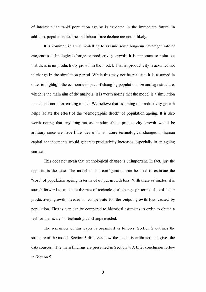
Adult generations (i.e. age groups 20-24, 25-29, …, 100-104) optimise their
consumption/saving patterns. A household’s optimization problem consists of
choosing a profile of consumption over the life cycle by maximizing a CES type inter-
temporal utility function that is subject to lifetime budget constraint. Inter-temporal
preferences of an individual born at time t are given by:
(5)
20
4
1
,, )(1
1
1
1k kgktkgkt
k
CusrU
0 < θ < 1
where “C” denotes consumption, “ ” is the pure rate of time preference and “θ” is
the inverse of the constant inter-temporal elasticity of substitution. Future
consumption is discounted by unconditional survival rate, “usr”, which is the
probability of survival up to the age “g+k” and may be written:
(6) usr kgkt , = mgmt
k
m sr ,0
where “srt+m,g+m” denotes the age/time-variable conditional survival rate between
periods “t+m” and “t+m+1” and between ages “g+m” and “g+m+1”
In is important to note that a “period” in the model corresponds to five years
and a unit increment in the index, “k”, represents both the next period, “t+k”, and, for
this individual, a shift to the next age group, “g+k”.
The household is not altruistic. It does not leave intentional bequests to
children. However, it leaves unintentional bequests due to uncertainty of life duration.
The unintentional bequests are distributed through a perfect annuity market, as
8
described theoretically by Yaari (1965). This idea was implemented in an OLG
context by Boersch-Supan et al. (2006).
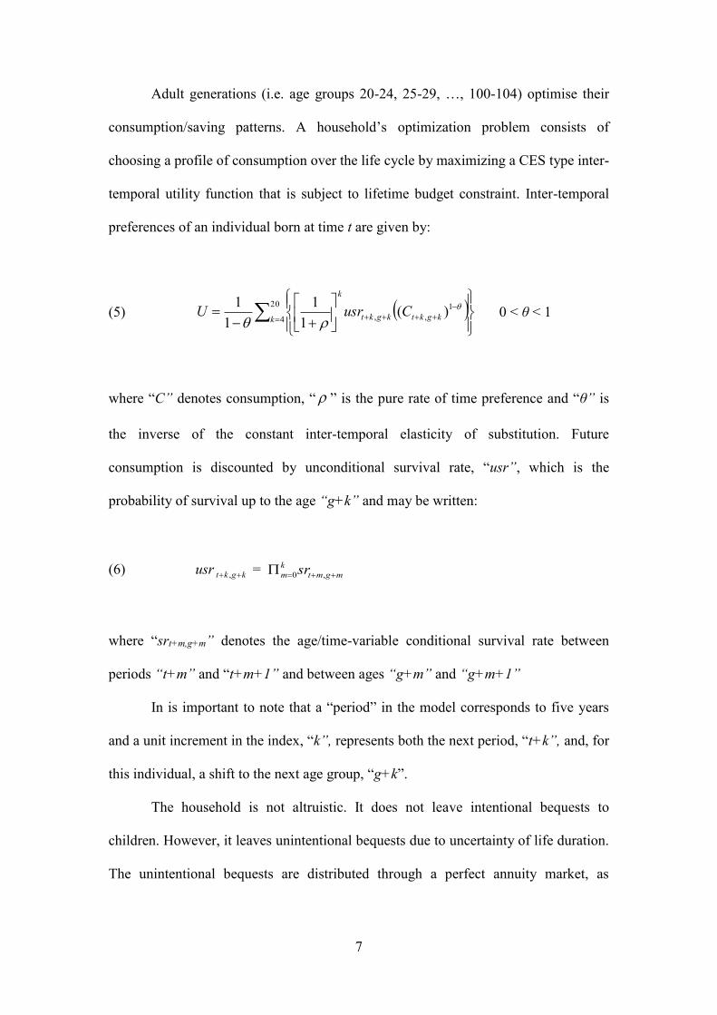
Given the assumption of a perfect annuity market, the household’s dynamic
budget constraint takes the following form:
(7)
gtgtt
K
tgtgtt
L
t
L
gt
gt
gt CHARiTRFPensCtrYsr
HA ,,,,,
.
1,1 1111
where “Ri” is the rate of return on physical assets, “τK” is the effective tax rate on
capital, “τL” is the effective tax rate on labour, “Ctr” is the contribution to the public
pension system, “YL” is labour income and “Pens” is pension benefits. The intuition
behind the term “1/sr” is that the assets of those who die during the period “t” are
distributed equally between their peers. Therefore, if the survival rate at time “t” in
age group “g” is less than one, then at time “t+1” everyone in their group has more
assets. That is, they all receive an unintentional bequest through the perfect annuity
market.
Labour income is defined as:
(8) ggt
L
gt LSEPwY ,
where “LS” is the exogenous supply of labour. It is assumed that labour income is a
function of the individual’s age-specific productivity. In turn, it is assumed that these
age-specific productivity differences are captured in age-earnings profiles. These
profiles, “EP”, are quadratic functions of age:
9
(9) 2)()( ggEPg , γ, λ, ψ ≥ 0
with parametric values estimated from micro-data (as discussed below). Retirees’
pension benefits are assumed to be the same across all generations and stay constant
in real terms.
Differentiating the household utility function with respect to its lifetime
budget constraint yields the following first-order condition for consumption,
commonly known as Euler’s equation:
(10)
gtt
K
tgt C
RiC ,
1
111,1
)1(
11
It is important to note that survival probabilities are present in both the utility
function and the budget constraint. Therefore, they cancel each other out and are not
present in the Euler’s equation.
2.3 Investment and Asset Returns
Migrants in any period are assumed to own the same level of assets the
domestic population of the same age. This implies that when net-migration is positive,
migrants’ assets add to the stock of capital. Therefore the motion law of capital stock,
“Kstock”, takes into account depreciation and assets of newly arrived migrants:
(11) 1,11,11 )1( gtg gtttt NMHAKstockInvKstock

10
where “Inv” represents investment, “δ” is the depreciation rate of capital, “HA” is
the level of household assets and “NM” is the level of net-migration.
Financial markets are fully integrated implying that financial capital is
undifferentiated so that interest rate parity holds. Let “Ri” be the rate of return on
physical assets. It can be defined as the rental rate minus the depreciation rate:
(12) )1(1 tt reRi
2.4 Government Sector
Currently Scotland has only limited tax-raising powers. For the majority of
spending, the Scottish Government receives a so-called “block grant” from the UK
Government. This grant is calculated based on the “Barnett Formula”, which takes
into account both the contributions of each region to tax revenue and the demand for
services. In our model, the revenue side of the government budget transfer on a
decomposition of the block grant calculated by the Scottish Government. Income and
consumption tax revenues are differentiated, as well as income from government
assets. The difference between government revenues and government expenditures –
net fiscal balance – in the model closes the government budget constraint. We call this
variable UK transfer, “UKTRF”, because in recent years this balance has been
negative, i.e. Scotland received a larger grant from the UK Government than was its
contribution to the centralised budget. Consequently government budget constraint is
defined as:
(13)
g
gtgtgtttt
ttt
g
gt
C
gt
C
tggtt
L
tgt
PensTRFPopGovHGovEGov
UKTRFGARiCPLSEPwCtrPop
,,,
,,,,

11
where “C” is the effective tax rate on consumption, “GA” is value of government
assets, “GovE” is public expenditures on education, “GovH” is public expenditures
on health care and “Gov” is public expenditures on other sectors (e.g. transport). The
left-hand side of this equation shows tax revenues from different sources, the interest
income from government assets and the transfers received from the UK government.
The right hand side of the equation refers to government expenditures and transfers to
households. Note that the representative household of generation “g” at time “t”
represents a specific cohort of size “ gtPop , ”. The size of each cohort must be taken
into account when computing total tax revenues and transfers to households in a
specific period of time. Note that the pension program is part of the overall
government budget.
Public expenditures on health and education are age-dependent. They are fixed
per person of a specific age. More specifically, “ASHEPCg” is age-specific health
expenditure per-person and “ASEEPCg” is age-specific education expenditure per-
person. Therefore, total public expenditure in these categories depends not only on the
size of the population but also on its age structure:
(14) 𝐺𝑜𝑣𝐻𝑡 = ∑ 𝑃𝑜𝑝𝑡,𝑔𝐴𝑆𝐻𝐸𝑃𝐶𝑔𝑔
(15) 𝐺𝑜𝑣𝐸𝑡 = ∑ 𝑃𝑜𝑝,𝑡,𝑔𝐴𝑆𝐸𝐸𝑃𝐶𝑔𝑔
Other types of public expenditures, “GEPC”, are assumed to be age-invariant. That is,
they are fixed per-person and hence total expenditure, “Gov”, depends only on the
size of the total population, “TPop”.

12
(16) 𝐺𝑜𝑣𝑡 = 𝑇𝑃𝑜𝑝𝑡 𝐺𝐸𝑃𝐶
2.5 Market and Aggregation Conditions
The model assumes that all markets are perfectly competitive. The equilibrium
condition for the goods market is that Scotland’s output, together with return on
foreign assets, “FA”, and transfers from RUK, must be equal to total demand
originating from consumption, investment and government spending:
(17) tttt
g
gtgttttt GovEGovHGovInvCPopUKTRFFARiY ,,
The demand for labour is equal to the supply:
(18) g
gggtt EPLSPopL ,
and the stock of capital accumulated in period “t” is equal to the demand expressed
by a firm:
(19) tt KKstock
The capital market is assumed to be in equilibrium. The total stock of private
wealth, “HA”, and government assets, “GA”, accumulated at the end of period “t”
must be equal to the value of the total stock of capital and foreign assets at the end of
period “t”:
13
(20) tt
g
tgtgt FAKstockGAHAPop ,,
Note that the current account can be derived from this model as the
difference between national savings and domestic investment:
(21)
Investment Domestic
1
Savings Private
1,1,1,11,1
tt
g
gtgt
g
gtgtt KstockKstockHAPopHAPopCA
Alternatively, the current account is either given as the trade balance plus the
interest revenues from net foreign asset holdings, or as the difference between
nominal GNP (i.e. GDP including interest revenues on net foreign assets) and
domestic absorption
3. Calibration
The model is calibrated using 2006 data for Scotland (where available). The
2006 year is chosen to avoid the effects of the financial crisis, which had a strong
negative impact on the performance of the Scottish economy and government
finances. The data for demographic shock is taken from the “official” population
projections carried out by the Office of National Statistics (discussed further below).
Population projections are used for calibration of fertility, survival and migration rates
used in the model.
The macro side of the model is calibrated base on aggregated 2006 social
accounting matrix (SAM). Data on public finances and GDP are taken from 2006-07
Government Expenditure and Revenue Scotland Report (GERS) (Scottish
Government, 2008). The estimate used assumes that North Sea revenues are

14
distributed on a geographical share basis. Effective wage income and consumption tax
rates are calculated from the corresponding government revenue category and
calibrated tax base i.e. total employment income and aggregate consumption. The
total amount of pensions and other transfers is taken from the Department of Work
and Pensions, Benefit Expenditure by Country, Region and Parliamentary
Constituency. Based on this information the effective pension contribution rate and
the average size of pension benefits are calculated. For effective pension contribution
rate calculation it is assumed that the same contribution rate is paid on all wage
income. For average size of pension benefits the total amount of pension benefits is
divided by the total number of people of pension age. For simplicity it is assumed that
both males and females start receiving pension benefits at age 65.
The source of the labour market data is the Quarterly Labour Force Survey
(QLFS). To avoid single observation biases data for three quarters is used (i.e.
Q1:2008, Q1:2009 and Q1:2010). From these pooled data, parameters of the age-
specific productivity (earnings) profiles are estimated. These data are also used to
calculate age-specific labour force participation rates. For age-specific productivity
profiles, Mincer age-earnings regressions are estimated (Mincer, 1958).
There are no Scotland specific estimates of the age structure of government
spending on health and education. Data of this type for Scotland and the UK are under
construction and were not available at the time of writing. However, there is some
evidence that suggests that the age-specific structure of government expenditure has a
similar shape in high-income countries. Lee and Mason (2011) report National
Transfer Accounts for many countries and demonstrate that age-specific profiles of
government spending on health and education are similar in high-income countries.
The specific estimates used in this paper are from the Canadian National Transfer
Accounts (see Zhang and Mérette, 2011). The majority of education spending occurs

15
between the ages 5-9 and 20-24. Health spending grows slowly until the age of 55-59
when it starts increasing much faster and accelerates after age 75-79. There is no
reason to believe that the “shape” of the Scottish profile would be radically different.
Capital share of the output (α) is set to 0.3. The (5-year) intertemporal elasticity of
substitution (1/γ) is set to 1.5.
There are three main steps in the calibration procedure. The first step consists
of using the information on output, capital and labour demands and the first-order
conditions of the firm problem to calibrate the scaling parameter for the productivity
function, plus wage and rental rates.
The second step is the most challenging involving equations pertaining to the
household’s optimisation problem, the equilibrium conditions in the assets and goods
markets to calibrate the rate of time preference and government expenditures on
sectors other than health and education (Gov). In other words, the (5-year) rate of time
preference is solved endogenously in the calibration procedure in order to generate
realistic consumption profiles and capital ownership profiles per age group, for which
no data are easily available. Capital ownership profiles must also satisfy the
equilibrium condition on the asset market. Public expenditures on other sectors (Gov)
is endogenously determined to close the budget constraint of the government and
ensures the equilibrium on the goods market. Note that the rate of time preference and
the inter-temporal elasticity of substitution together determine the slope of the
consumption profiles across age groups in the calibration of the model (when the
population is assumed to be stable). This is also the slope of the consumption profile
of an individual across his lifetime in the simulated model in the absence of
demographic shocks or economic growth.
The third and final step uses the calibration results of the first three steps to
verify the model is able to replicate the observed data corresponding to the initial
16
equilibrium. Only when the initial equilibrium is perfectly replicated with the
calibration solution can the model be used to evaluate the consequences of
demographic shocks associated with population ageing.
4. Findings
The baseline demographic scenario is the “official” 2010-based principal
population projection for Scotland (National Records of Scotland, 2011). This
projection is summarised in Figure 1 which shows the growth rates of key age groups.
According to this projection, by 2106 total population will increase by 22%, the
pension age population (65+) will increase by 127%; the children/youth population
(<20) will stay constant and the working age population (20-64) will stagnate during
this period with an increase of 1%. It is clear from this projection that significant
population ageing is expected.
Figure 2 reports simulated changes in output until 2106. Figure 3 shows
simulated changed in output per-person. The simulation suggests a reduction in output
per-person above 15% over the next 100 years. This corresponds to a considerable
welfare loss “caused” by population ageing.
With the model it is possible to use the results ex-post to approximate how
much total factor productivity growth is needed to compensate for the output loss
called by population ageing. The model suggests that productivity growth of about
15% is needed over the next 100 years just to keep output per-person constant. In
other words, productivity growth averaging around 0.14% per year is needed.
This estimated rate of future growth is well below recent trend productivity
growth in the UK. Data from the EU KLEMS project suggest that productivity growth
over the past two decades has averaged 2% per years (see O’Mahony and Timmer,

17
2009). Therefore, the analysis carried out in this paper suggests that about 7% of
(recent) historically observed productivity growth is required to counteract the
negative effect of population ageing on output per person. This is a significant change
and suggests that a “technological leap” will be needed that leads to a large increase
in productivity. Of course, the key unanswered question is what will cause such a big
change?
5. Concluding Comment
This paper developed an overlapping generations (OLG) computable general
equilibrium (CGE) model in order to evaluate the macro-economic impacts of
population ageing in Scotland. The model is particularly well suited to this task since
its OLG structure explicitly allows for the incorporation of ageing effects related to
age-specific labour force participation, age-specific productivity differences and age-
specific government expenditures. Population ageing is associated with lower output
per-person suggesting that it is welfare reducing. It was demonstrated that the
technical change needed to counteract this loss in welfare is considerable.

18
References
Auerbach, A. and Kotlikoff, L., 1987. Dynamic Fiscal Policy. Cambridge University
Press, Cambridge.
Bommier, A. and Lee, R.D., 2003. Overlapping generations models with realistic
demography. Journal of Population Economics, 16, 135-160.
Boersch-Supan, A., Ludwig, A. and Winter, J., 2006. Aging, pension reform and
capital flows: a multi-country simulation model. Economica, 73, 625-658.
Boersch-Supan, A., 2003. Labour market effects of population ageing. Labour, 17
(Special Issue), 5-44.
Burfisher, M.E., 2011. Introduction to Computable General Equilibrium Models.
Cambridge University Press, Cambridge.
Dixon, B. and Jorgenson, D., 2012. Handbook of Computable General Equilibrium
Modelling. North Holland, Amsterdam.
Fossati, A. and Wiegard, W., 2001. Policy evaluation with computable general
equilibrium models. Routledge, London.
Fougere, M. and Merette, M., 1999. Population ageing and economic growth in seven
OECD countries. Economic Modelling, 16, 411-427.
Fougere, M., Mercenier, J. and Merette, M., 2007. A sectoral and occupational
analysis of population ageing in Canada using a dynamic CGE overlapping
generations model. Economic Modelling, 24, 690-71.
Fougère, M., Harvey, S., Mérette, M. and Poitras, F., 2004. Ageing population and
immigration in Canada: an analysis with a regional CGE overlapping
generations model. Canadian Journal of Regional Science, 27, 209-236.
Giesecke, J.and Meagher, G.A., 2009. Population ageing and structural adjustment.
CoPS/IMPACT Working paper G-18. Monash University, Adelaide

19
Hosoe, N., Gasawa, K. and Hashimoto, H., 2010. Textbook of Computable General
Equilibrium Modeling: Programming and Simulations. Palgrave Macmillan,
London.
Lee, R. and Mason, A., 2011. Population ageing and the generational economy: a
global perspective. Edward Elgar, Cheltenham.
Mérette, M. and Georges, P., 2010. Demographic changes and gains from
globalisation: an analysis of ageing, capital flows and international trade,
Global Economy Journal, 10, online article.
Mincer, J., 1958. Investment in human capital and personal income distribution.
Journal of Political Economy, 66, 281-302.
National Records of Scotland, 2011. Projected Population of Scotland (2010-based).
National Population Projections by Sex and Age, with UK and European
Comparisons. National Records of Scotland, Edinburgh.
O’Mahony, M. and Timmer, M. 2009. Output, Input and Productivity Measures and
the industry level: The EU KLEMS Database. Economic Journal, 119 (538),
F374-F403
Scottish Government, 2008. 2006-07 Government Expenditure and Revenue
Scotland. Scottish Government, Edinburgh.
Weil, D., 1997, The economics of population ageing, in: M. Rosenzweig, Stark, O.
(Eds.), Handbook of Population Economics, Volume 1, Part B, North Holland,
Amsterdam, pp. 967-1014.
Yaari, M.E., 1965. Uncertain lifetime, life insurance, and the theory of the consumer.
Review of Economic Studies, 32, 137-160.
Zhang, and Merette, M, 2011. National transfer accounts: the case of Canada,
manuscript. University of Ottawa, Ottawa.

20
-20%
0%
20%
40%
60%
80%
100%
120%
140%
2011 2016 2021 2026 2031 2036 2041 2046 2051 2056 2061 2066 2071 2076 2081 2086 2091 2096 2101 2106
Figure 1Projected Change in Scottish Population by Age Groups, 2011-2106
<20 20-64 65+ Total
0.0%
1.0%
2.0%
3.0%
4.0%
5.0%
20
06
20
11
20
16
20
21
20
26
20
31
20
36
20
41
20
46
20
51
20
56
20
61
20
66
20
71
20
76
20
81
20
86
20
91
20
96
21
01
21
06
Figure 2
Simulated Changes in Output, Scotland, 20011-2106
with age-specific features
-20%
-15%
-10%
-5%
0%
5%
10%
15%
20%
20
06
20
11
20
16
20
21
20
26
20
31
20
36
20
41
20
46
20
51
20
56
20
61
20
66
20
71
20
76
20
81
20
86
20
91
20
96
21
01
21
06
Figure 3
Simulated Changes in Output Per-person, 2011-2106
GDP per-person with age-specific effects

21