popov statbility

8/12/2019 popov statbility

http://slidepdf.com/reader/full/popov-statbility 1/6



( ) ( 12 x f x g )−−=ψ (8)

then the Jacobian matrix of this system is (where we have to

give for the coordinate of singular point

)

21 ; x x

0 ; 2101 == x x x

( )⎥⎥⎦

⎤

⎢⎢⎣

⎡

∂∂

∂∂=

21

0

10

x x

ψ ψ xJ (9)

and then following equations represents the linearization of

the nonlinear equations about the equilibrium point

( )

( ) ψψ

d

d

d

d

22

1011

2

2101

x x

x x x

xt

x x xt

∂

∂+−

∂

∂=

=−

(10)

2211 x x x ∂∂∂

These equation

Table I: Linearized equations of nonlinear systems

NoEquation of nonlinear

systemψ

Singular

pointsLinearized equation

1 0=+′+′′ y yby y r 121 x xbx r −− [ ]0;0 0=+′′ y y

2 0=+′+′′ cy yby ya r 121 x

a

c x x

a

b r −− [ ]0;0 0=+′′ ya

c y

[ ]0;0

1012

21

ψψψ x x x x

x x

∂+

∂−

∂=′

=′⇒

s correspond to the linearized second order

0=+′+′′ ya

c y

a

b y

3 02 =++′+′′ dycy yb ya 2112 x

a

d x

a

c x

a

b−−−

⎥⎦

⎤⎢⎣

⎡− 0;

d

c0=+−′+′′

a

c y

a

c y

a

b y

4 0=++′+′′ t dycy yb ya t x

a

d x

a

c x

a

b112 −−− [ ]0;0 0=+′+′′ y

a

c y

a

b y

5 0=+′+′+′′ dy ycy yb yar 1212 x

a

d x x

a

c x

a

b r −−− [ ]0;0 0=+′+′′ ya

d y

a

b y

[ ]0;0 0=+′+′′ ya

d y

a

b y

6 02 =++′+′+′′ eydy yc yb ya r 21122 x

a

e x

a

d x

a

c x

a

b r −−−−

⎥⎦

⎤⎢⎣

⎡− 0;

e

d 0=−′+′′ y

a

d y

a

b y

7 0=++′+′+′′ t r eydy yc yb ya t r x

a

e x

a

d x

a

c x

a

b1122 −−−−

[ ]0;0 0=+′+′′ ya

d y

a

b y

8 ( ) 0=+′++′′ cy ynymb ya r ( ) 121 x

a

c xnxm

a

b r −+− [ ]0;0 0=+′+′′ ya

c ym

a

b y

9 ( ) 0=+′++′′

cy ynymyb ya

qr p

( ) 1211 xa

c

xnxmxa

b qr p −+− [ ]

0;0 0

=+′′ ya

c

y

Proceedings of the World Congress on Engineering and Computer Science 2009 Vol IIWCECS 2009, October 20-22, 2009, San Francisco, USA

ISBN:978-988-18210-2-7 WCECS 2009



( )

( )[ ] ( ) 22

2112

21221

22

11

21

12122

,

x x x x x x x x

x x

V x

x

V x xV

+−=−+−+=

=′∂

∂+′

∂

∂=′

The function V ́ is negative semidefinite (because for x2

= 0 the function V ́ is for arbitrary x1 equals zero) and the

system is globally stable.

III. POPOV CRITERION

The Popov criterion is considered as one of the most ap-

propriate criteria for nonlinear systems and it can be com-

pared with the Nyquist criterion for linear systems [4].

However there are reservations that relate to the very es-

sence, correctness and reliability of the criterion. It is nec-

essary to emphasise that this criterion is reliable, but the

conditions of its appl. should be clearly specified in advance.

Table II: Lyapunov´s functions for second-order systems

No Equation of system Restriction Lyapunov function V

1 0=+′+′′ cy yb ya -

2 0=+′+′′ cy yby ya qr r even q odd

22

21 x x

a

cV +=

3 0=+′+′′t qr

cy yby ya r even q,t odd

4 ( ) 0=+′++′′ t q sr cy ynymyb ya r,s even q,t odd

5 ( )( ) 0=+′+′++′′ t k q sr cy y f yenymyb ya r,s even k,q,t odd

22

11

1

12 x x

t a

cV t +

+= +

Table III: Lyapunov´s functions for third-order systems

No Equation of system Restriction Lyapunov function V

1 0=′+′′+′′′ r m yb ya y a,b>0

m,r odd23

12

1

2 x x

r

bV

r ++

= +

2 0=′+′′+′′′+′′′ ht r nm ye y yb y ya y

a,b,e>0

m,r odd

n,t,h even

23

12

1

2 x x

h

eV

h ++

= +

3 0=′+′′′+′′′+′′′ ht sr pnm ye y y yb y y ya y

a,b,e>0

h,m,r odd

n,p,s,t even

23

12

1

2 x x

h

eV h +

+= +

4

01 =′′′+

+′′′+′′+′′′+′′′

− z

ut sr pnm

y y yd

y y yc y yb y ya y

a,b,c,d>0

m,p,s,z odd

n,r,t,u even

23

12

1

2 x x

d V z +

+= +

5

0=′+

+′′′+′′+′′′+′′′

h

ut sr pnm

ye

y y yc y yb y ya y

a,b,c,e>0

m,p,s,h odd

n,r,t,u even

23

12

1

2 x x

h

eV

h ++

= +

6

01 =′+′′′+

+′′′+′′+′′′+′′′

− h z

ut sr pnm

ye y y yd

y y yc y yb y ya y

a,b,c,d,e>0

h,m,p,s,z odd

n,r,t,u even 23

12

11

1

2

1

2

x xh

e

x z

d V

h

z

++

+

++

=

+

+

701 =−′+′′′+

+′′′+′′+′′′+′′′

− y y y y y

u yt y s yc y ybn ym ya y r p

a,b,c>0

m,p,s odd n,r,t,u

even( ) 2

32

21 x x xV +−=

801 =+′+′′′+

+′′′+′′+′′′+′′′

− fy ye y y yd

y y yc y yb y ya y ut sr pnm

a,b,c,d,e>0f<0

d

f e

2=

m,p,s odd

n,r,t,u even

23

2

21 x xd

f xd V +⎟⎟

⎠

⎞⎜⎜⎝

⎛ +=


ISBN:978-988-18210-2-7 WCECS 2009



Fig. 1 shows the system configuration with one nonlinear

element and a linear part with the transfer function G( s) that

can include all linear elements. It shows the nonlinearity that

is single-valued, time–invariant and constrained to a hatch

sector bounded by slopes k that is assumed to satisfy: for the

case when all poles of G( s) are inside the left-half plane

( )∞<≤≤ k

e

e f 0 ,

for the case when G( s) has poles on the imaginary axis (the

so-called critical case)

( )∞<≤< k

e

e f 0

.

Fig.1: Non-linear control circuit and characteristic of

nonlinear element

For the case that G( s) has poles only inside the left-half

s-plane, the static characteristic can be zero both in the be-

ginning and out of the beginning. For the case when G( s) has

poles on the imaginary axis, it must not be zero out of the

beginning.

A nonlinear circuit with a transfer function of the linear

part G( s) and with the nonlinear element (with the above

described nonlinearity) is globally asymptotically stable

when an arbitrary real number q (> 0 or = 0 or < 0) exists

where for every ω ≥ 0 the following inequality is completed

( ) ( )[ ] 01

ωω1Re >++k

jGq j (14)

The Popov criterion can be – for more convenience – ap-

plied graphically in the G ( jω)-plane. Let us apply a modified

frequency response function G*( jω), defined

for (15)( ) ( )

( ) ( )ωIm.ωωIm

ωReωRe

jG jG

jG jG

=

=

∗

∗

0ω ≥

and we obtain the graphical interpretation of the Popov cri-terion for global asymptotic stability (GAS): The sufficient

condition for GAS of nonlinear circuit is that the plot of

G*( jω) should lie entirely to the right of the Popov line which

crosses the real axis at -1/k at a slope 1/q (q is an arbitrary

real number) .

In this contribution table III shows the commonly used

nonlinear circuits (with stability being solved). The table has

been constructed for the circuits with different transfer

function G( s).There is an algebraic solution to the inequality

(14) on condition that:

0 ≤ k < ∞ (only for poles G( s) inside the left-half of s-plane);

0 < k < ∞ (also for poles G( s) on the imaginary axis); a, b >0; ω... for every value from 0 to ∞ ; q...arbitrary.

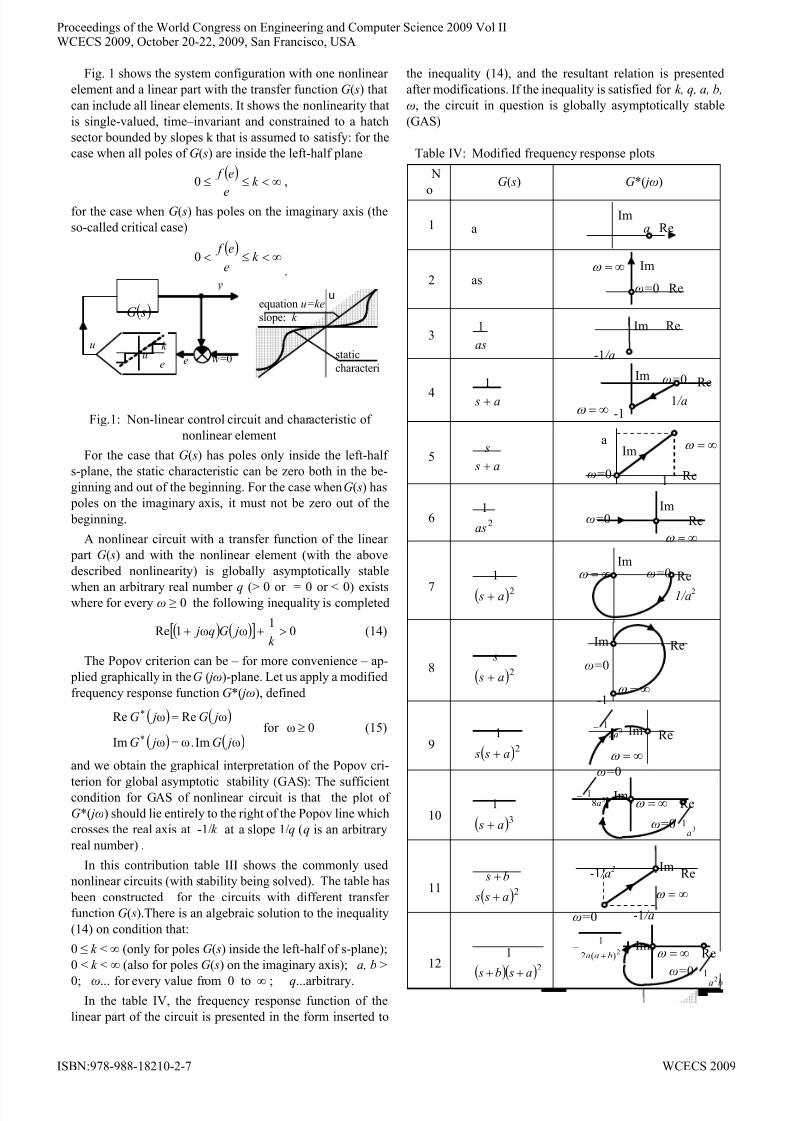
In the table IV, the frequency response function of the

linear part of the circuit is presented in the form inserted to

the inequality (14), and the resultant relation is presented

after modifications. If the inequality is satisfied for k, q, a, b,

ω, the circuit in question is globally asymptotically stable

(GAS)

Table IV: Modified frequency response plots

N

o

G( s) G*( jω)

1 a

2 as

3as

1

4a s +

1

∞=ω

5a s

s

+

6 2

1

as

7( )2

1a s +

8( )2

a s

s

+

9( )2

1

a s s +

10( )3

1

a s +

11( )2

a s s

b s

+

+

12 ( )( )2

1

a sb s ++

Im

ReIm

-1 /a

Im

Re1 /a

ω

=0

-1

Re1ω=0

∞=ω a

∞=ω

ReIm

ω=0

Re

Im

1/a2

ω

=0∞=ω

Im Re

-1

ω=0

∞=ω

Im Re

ω=0

∞=ω

321

a−

ImRe

ω=0

∞=ω 38

1a

−

31

a

Im-1 /a2

ω=0 -1 /a

∞=ω

Re

ImRe

ω=0

∞=ω 2)(2

1

baa +−

ba21

Im

∞=ω

Re

Im

ω=0

Rea

u

equation u=ke

slope: k

static

characteri

( ) sG

u

eeu w=0

k


ISBN:978-988-18210-2-7 WCECS 2009



for every value k . If it is not the case, then it is possible to

determine for which k circuit is GAS or that it is not for any k

(this calculation is illustrated in the table). Therefore the table

will allow us to directly determine the stability of the

nonlinear circuit with the transfer function G( s) and the

nonlinearity that satisfies the slope k . Table V illustrates the

modified frequency response plots enabling us graphic solu-

tions to stability.

IV. CONCLUSION Stability analysis of nonlinear control systems is difficult

task in engineering practice. This paper can help to solve the

problem. The describe methods creates tables and graphs for

three methods of stability analysis.First method is method of linearization. The table

includes the nonlinear equations and directs their linear ap-

proximation. Second method is Lyapunov direct method.

The table contains Lyapunov functions for usually used

control circuits second and third-order. The last method is

Popov criterion. The table will allow us to directly determine

the stability of the nonlinear circuit with the transfer function

G( s) and the nonlinearity that satisfies the slope k .

R EFERENCES

[1] R. Iserman, “Digital Control Systems”, Springer , Berlin, 1989

[2] W. S. Levine, “The Control Handbook ”, CRC Press, Inc., Boca Raton,

Florida 1996

[3] I. Svarc, R. Matousek, “How and when to use Popov and circle criteria

for stability”, In Proceedings of the ICCC ’2008, Sinaia (Romania),

2008, pp. 663-666. ISBN 978-973-746-897-0

[4] I. Svarc, “Stability analysis of nonlinear control systems using lin-

earization”, In Proceedings of 5th ICCC’2004, Zakopane, pages 25 - 30

[5] I. Svarc, “A new approach to graphs to stability of nonlinear controlsystems”, Journal Elektronika, Warsaw, No 8-9/2004, pages 18-22

[6] N. Sidorov, B. Loginov, A. Sinitsyn, M. Falaleev, “Lyapunov-Schmidt

Method in Nonlinear analysis and Applications”, Kluwer Academic

Publisher , 2002

Table V: Results of stability analysis by Popov´s criterion

No G( s) G( jω) in inequality (14)

( ) ( )[ ] 01

1Re >++k

jGq j ω ω Solution of (14)

Conditions of

stability

1 a a ka+1 > 0 GAS for every k

2 as ajω 1 - k ω3q > 0 GAS for every k

3as

1

ω a j

1− qk + a > 0 GAS for every k

4a s +

1

2222ω

ω

ω +−

+ a j

a

a

02

22

>+

+++

ω

ω aqak GAS for every k

5a s

s

+

2222

2

ω

ω

ω

ω

++

+ a

a j

a

( )

0

1

2

22

>+

++−

ω

ω aaqk GAS for every k

6 2

1

as

2

1

ω a− 2

ω ak < not stable for

arbitrary k

7( )2

1

a s +

( ) ( )222222

22 2

ω

ω

ω

ω

+−

+

−

a

a j

a

a

( )

( ) 0

12

222

22

>++

++−

ω

ω

a

kaaqk GAS for every k

8( )2

a s

s

+

( ) ( )222

32

222

22

ω

ω ω

ω

ω

+

−+

+ a

a j

a

a

( )( ) 0

2222

222

>++

+−+

ω

ω ω

a

aqak GAS for every k

9( )2

1

a s s +

( ) ( )222

22

222

2

ω ω

ω

ω +

−+

+

−

a

a j

a

a…

GAS for

k < 2a3

10 ( )31

a s + ( ) ......1

3 =+ a jω … GAS fork < 8a3

11( )2

a s s

b s

+

+

( )...

2 =

+

+

a j j

b j

ω ω

ω

32234

2456

28104

6124

abbabaa

babaak

−+−

+−−>

12( )( )2

1

a sb s ++

( )( )...

12 =

++ a jb j ω ω

( )2

4322345 281282

ba

abbababaak

+

++++<


ISBN:978-988-18210-2-7 WCECS 2009

popov statbility

Documents

Transcript of popov statbility