Poor Families, Poor Neighborhoods: How Family · PDF filePoor Families, Poor Neighborhoods:...
63
Transcript of Poor Families, Poor Neighborhoods: How Family · PDF filePoor Families, Poor Neighborhoods:...

Poor Families, Poor Neighborhoods: How Family Poverty Intensifies the Impact of
Concentrated Disadvantage on High School Graduation
Geoffrey T. Wodtke University of Michigan
Felix Elwert
University of Wisconsin-Madison
David J. Harding University of Michigan
Population Studies Center Research Report 12-776 September 2012
Corresponding Author: Geoffrey T. Wodtke, Population Studies Center, Institute for Social Research, University of Michigan, 426 Thompson Street, Ann Arbor, MI 48106. [email protected] Acknowledgements: The authors thank Daniel Almirall, Robert Sampson, Jeffrey Timberlake, and the University of Michigan Inequality Working Group for helpful discussions. This research was supported by the National Science Foundation Graduate Research Fellowship under Grant No. DGE 0718128 and by the National Institute of Child Health and Human Development under Grant Nos. T32 HD007339 and R24 HD041028 to the Population Studies Center at the University of Michigan.

Effects of Neighborhood Disadvantage among Poor Families 2
ABSTRACT
Theory suggests that the effects of disadvantaged neighborhoods on child educational outcomes may depend on a family’s economic resources as well as the timing of neighborhood exposures during the course of child development. However, most previous research assumes that disadvantaged neighborhoods have the same effects on all children regardless of their family resources, and few prior studies specifically analyze the timing of exposure to different neighborhood conditions across the early life course. This study extends research on neighborhood effects by investigating how timing of exposure to disadvantaged neighborhoods during childhood and adolescence affects high school graduation and whether these effects vary across families with different economic resources. Results based on novel counterfactual methods for time-varying treatments and time-varying effect moderators indicate that exposure to disadvantaged neighborhoods, particularly during adolescence, has a strong negative effect on high school graduation, and that this deleterious effect is much more severe for children from poor families. The severe impact of spatially concentrated disadvantage on children from poor families suggests that ecological socialization models of neighborhood effects must account for the interactions between nested social contexts like the family environment and local neighborhood, as well as for the dynamic coevolution of these contexts over time.
Effects of Neighborhood Disadvantage among Poor Families 3
INTRODUCTION
Since the publication of Wilson’s (1987) influential treatise on urban poverty, researchers
have worked to better understand the spatial dimensions of stratification processes, focusing
especially on the impact of concentrated neighborhood disadvantage on educational attainment.
Disadvantaged neighborhoods are thought to have a harmful impact on educational attainment
because resident children are socially isolated from successful role models, lack access to
institutional resources, are exposed to a variety of environmental health hazards, and must
navigate heterogeneous subcultures with conflicting views about the utility of formal schooling
(Anderson 1999; Brooks-Gunn, Duncan, and Aber 1997; Harding 2010; Jencks and Mayer 1990;
Massey 2004; Massey and Denton 1993; Sampson 2001; Wilson 1987; Wilson 1996). Although
earlier empirical evidence is mixed—some studies report no effect of neighborhood context on
educational attainment (e.g., Ginther, Haveman, and Wolfe 2000) and others find only small
effects (e.g., Aaronson 1998; Brooks-Gunn, Duncan, Klebanov, and Sealand 1993; Crane 1991;
Harding 2003)—more recent research documents strong neighborhood effects on educational
outcomes (Crowder and South 2010; Sharkey and Elwert 2011; Wodtke, Harding, and Elwert
2011).
Few studies, however, investigate whether the impact of neighborhood context depends
on, or is moderated by, other circumstances of a child’s life. In particular, prior research typically
assumes that the effects of neighborhood context are the same for all children, regardless of their
families’ economic resources (e.g., Ginther, Haveman, and Wolfe 2000; Harding 2003; Wodtke,
Harding, and Elwert 2011). Yet several sociological theories strongly suggest that the
socioeconomic position of the family should moderate the impact of neighborhood context.
Neighborhood-effect moderation occurs when individual or family characteristics dampen or
amplify the effect of some neighborhood treatment. For example, compound disadvantage theory
contends that family poverty intensifies the harmful effects of neighborhood deprivation because
children from poor families must rely more heavily on neighborhood networks, adults, and

Effects of Neighborhood Disadvantage among Poor Families 4
institutional resources than children from nonpoor families (Jencks and Mayer 1990; Wilson
1987; Wilson 1996). By contrast, relative deprivation theory posits that the effects of
disadvantaged neighborhoods are less severe among children in poor families because they lack
the personal resources needed to capitalize on social advantages available in more affluent
neighborhoods (Crosnoe 2009; Jencks and Mayer 1990). Previous studies that consider only the
marginal, or population average, effects of neighborhood context may obscure potentially
divergent consequences of growing up in disadvantaged neighborhoods among different
subgroups of children.
The consequences of living in disadvantaged neighborhoods also likely depend on the
timing of exposure during the course of development. Theories about the impact of concentrated
disadvantage on child development suggest that different neighborhood exposure trajectories
may have different effects on child educational outcomes, where, for example, those perspectives
emphasizing peer socialization mechanisms anticipate more pronounced effects of adolescent,
rather than early childhood, exposure to neighborhood disadvantage. Recent research shows that
it is critically important to account for duration of exposure to disadvantaged neighborhoods
(Crowder and South 2010; Wodtke, Harding, and Elwert 2011), but prior studies do not examine
how effects of neighborhood deprivation vary across different development periods. If
neighborhood effects are different between childhood and adolescence, then previous studies
provide an incomplete assessment of the developmental process through which neighborhoods
impact individuals. Neighborhood context is not a static feature of a child’s life: families move,
and neighborhoods change, exposing many children to different neighborhood conditions
throughout the course of development (Quillian 2003; Timberlake 2007).
This study investigates whether neighborhood effects are moderated by family economic
resources and whether these effects depend on the timing of neighborhood exposures during
different developmental stages. Specifically, it examines how exposure to disadvantaged
neighborhoods during childhood versus adolescence affects the chances of high school

Effects of Neighborhood Disadvantage among Poor Families 5
graduation among different subgroups of children defined in terms of the resources available to
their families over time. We focus on high school graduation because it is a critical educational
transition and essentially a precondition for economic security as an adult (Rumberger 1987).
Analyses of neighborhood-effect moderation are complicated by a number of
methodological difficulties. First, estimating neighborhood effects without regard for effect
moderation is itself a difficult endeavor because families dynamically select into and out of
neighborhoods on the basis of time-varying covariates. For example, parental marital status
affects future neighborhood attainment; in turn, where the family lives affects subsequent marital
events. In technical terms, parental marital status is a time-varying confounder affected by past
treatment. Conventional regression adjustments for observed time-varying confounders affected
by past neighborhood conditions cannot consistently estimate neighborhood effects (Wodtke,
Harding, and Elwert 2011).
Second, estimating how neighborhood effects are moderated by family economic
resources is even more complicated because the resources available to a family at a given point
in time depend in part on where the family lived in the past. If, for example, we are interested in
the effects of adolescent exposure to disadvantaged neighborhoods among subjects whose
families are poor during this developmental stage, we must contend with the problem that
neighborhood conditions during childhood in part create the subgroup of interest (poor families)
during adolescence. Appropriate handling of endogenous effect moderators, such as family
resources, presents an additional challenge above and beyond the problem of adjusting for time-
varying confounders affected by prior neighborhood context. Methods designed to appropriately
adjust for time-varying confounders in models for the marginal, or population average, effects of
treatment—for example, marginal structural models estimated by inverse probability of
treatment weighting (Wodtke, Harding, and Elwert 2011)—are not appropriate for analyzing
effect moderation by endogenous time-varying covariates.

Effects of Neighborhood Disadvantage among Poor Families 6
To overcome these problems, we use a two-stage regression-with-residuals estimator for
structural nested mean models to assess the effects of different neighborhood exposure
trajectories conditional on the evolving economic position of the family (Almirall, McCaffrey,
Ramchand, and Murphy 2011; Almirall, Ten Have, and Murphy 2010; Robins 1994). Under
assumptions defined below, these methods provide for unbiased estimation of the moderated
effects of time-varying treatments when time-varying confounders and putative moderators are
affected by past treatment.
This study advances research on the educational effects of concentrated neighborhood
disadvantage by (1) delineating a counterfactual model for neighborhood effects that
incorporates both time-varying treatments and effect moderators and (2) estimating the effects of
exposure to disadvantaged neighborhoods during childhood versus adolescence for different
subgroups of children defined in terms of their family resource history. We begin with a brief
review of the theoretical mechanisms through which neighborhood disadvantage is thought to
impact high school graduation. Next, we discuss several theories positing that the effects of
neighborhood disadvantage depend on the economic position of the family and the
developmental timing of exposure. Then, we outline the dynamic neighborhood selection process
that complicates conventional regression analyses, present the structural nested mean model and
its two-stage regression estimator, and, with data from the Panel Study of Income Dynamics,
estimate the moderated effects of exposure to disadvantaged neighborhoods during childhood
versus adolescence on high school graduation.
Results indicate that exposure to disadvantaged neighborhoods, particularly during
adolescence, has a strong negative effect on the chances of high school graduation and that the
deleterious effect of adolescent exposure to disadvantaged neighborhoods is much more severe
among individuals whose families are poor during this developmental period. In other words, we
find that the subgroup of individuals living in poor families during adolescence is especially
vulnerable to the harmful effects of disadvantaged neighborhoods. We conclude that ecological
Effects of Neighborhood Disadvantage among Poor Families 7
socialization models must account for the interactions between nested social contexts like the
family and neighborhood, as well as for the dynamic coevolution of these contexts over time.
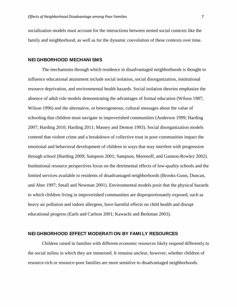
NEIGHBORHOOD MECHANISMS
The mechanisms through which residence in disadvantaged neighborhoods is thought to
influence educational attainment include social isolation, social disorganization, institutional
resource deprivation, and environmental health hazards. Social isolation theories emphasize the
absence of adult role models demonstrating the advantages of formal education (Wilson 1987;
Wilson 1996) and the alternative, or heterogeneous, cultural messages about the value of
schooling that children must navigate in impoverished communities (Anderson 1999; Harding
2007; Harding 2010; Harding 2011; Massey and Denton 1993). Social disorganization models
contend that violent crime and a breakdown of collective trust in poor communities impact the
emotional and behavioral development of children in ways that may interfere with progression
through school (Harding 2009; Sampson 2001; Sampson, Morenoff, and Gannon-Rowley 2002).
Institutional resource perspectives focus on the detrimental effects of low-quality schools and the
limited services available to residents of disadvantaged neighborhoods (Brooks-Gunn, Duncan,
and Aber 1997; Small and Newman 2001). Environmental models posit that the physical hazards
to which children living in impoverished communities are disproportionately exposed, such as
heavy air pollution and indoor allergens, have harmful effects on child health and disrupt
educational progress (Earls and Carlson 2001; Kawachi and Berkman 2003).
NEIGHBORHOOD EFFECT MODERATION BY FAMILY RESOURCES
Children raised in families with different economic resources likely respond differently to
the social milieu in which they are immersed. It remains unclear, however, whether children of
resource-rich or resource-poor families are more sensitive to disadvantaged neighborhoods.
Effects of Neighborhood Disadvantage among Poor Families 8
Competing social theories about neighborhood effect moderation—compound disadvantage
theory and relative deprivation theory—suggest starkly different scenarios.
Compound disadvantage theory posits that the detrimental impact of exposure to poor
neighborhoods is more severe for children who are also living in poor families (Jencks and
Mayer 1990; Wilson 1987; Wilson 1996). Family poverty itself is known to harm children’s
educational attainment (Duncan and Brooks-Gunn 1997; Duncan, Yeung, Brooks-Gunn, and
Smith 1998; Mayer 1997). Beyond this independent effect, family poverty is further thought to
exacerbate the effects of neighborhood disadvantage for several reasons. First, the social
networks of poor families are more often restricted to the local neighborhood than those of
nonpoor families (Jencks and Mayer 1990). By virtue of the limited geographic scope of their
social networks, children with poor parents may be more sensitive to the absence of successful
role models and the presence of “ghetto-related” subcultures in the local neighborhood (Wilson
1996). Without parents or resident adults to signal that socioeconomic advancement is possible,
children living in both poor families and disadvantaged neighborhoods may develop indelible
fatalistic sentiments about their life chances.
Second, in order to acquire the cultural skills that facilitate advancement in the formal
education system (Carter 2005), children with poor parents must rely more heavily on resident
adults and neighborhood institutions. By contrast, children with economically advantaged
parents can learn these skills at home and thus are less dependent on the local neighborhood.
Thus, if the neighborhood lacks role models and institutions to instill the requisite cultural skills,
then children in poor families will be most affected.
Finally, parents with greater economic resources may be able to “buy out” of the
potentially harmful effects of institutional resource deprivation in disadvantaged neighborhoods.
For example, nonpoor parents living in disadvantaged neighborhoods may be able to afford
higher-quality childcare outside the neighborhood, enroll their children in private schools or
other supplementary educational programs, and travel beyond the neighborhood to secure other
Effects of Neighborhood Disadvantage among Poor Families 9
goods and services that facilitate effective parenting. Children from poor families, on the other
hand, are likely more dependent on the institutional resources, or lack thereof, within the
neighborhood. For compound disadvantage theory, then, the negative educational effects of
residence in more versus less disadvantaged neighborhoods are hypothesized to be especially
severe for children in poor families and comparatively modest for children in nonpoor families.
In sharp contrast to compound disadvantage theory, relative deprivation theory, as it
relates to neighborhood effect moderation, contends that the impact of neighborhood
disadvantage is less severe for children in poor families than for children in nonpoor families
because a variety of social processes prevent poor children from realizing the benefits associated
with residence in more advantaged neighborhoods. Children in both poor and nonpoor families
are thought to have lower educational outcomes in disadvantaged neighborhoods, but children in
poor families are thought to benefit less than children in nonpoor families from residence in
more advantaged neighborhoods.
Because poor families lack disposable income, they may not be able to capitalize on the
availability of institutional resources in advantaged neighborhoods (Jencks and Mayer 1990). For
example, living in a neighborhood with quality childcare, high-end grocery stores, and many
recreational programs may be of little consequence to families that cannot afford these goods and
services. In this situation, residence in a more affluent neighborhood, relative to residence in a
disadvantaged neighborhood, may have little impact on children from poor families. By contrast,
children in nonpoor families, who can realize the benefits of access to neighborhood resources,
are expected to be more sensitive to their neighborhood context.
According to social psychological variants of relative deprivation theory, children
evaluate themselves, and are evaluated by resident adults, relative to their neighborhood or
school peers (Crosnoe 2009; Marsh 1987). Poor children living in more affluent neighborhoods,
then, may suffer stigmatization or develop negative self-perceptions that interfere with their
schooling. Nonpoor children in affluent neighborhoods do not suffer the harmful psychological

Effects of Neighborhood Disadvantage among Poor Families 10
and emotional effects of relative deprivation. Thus, when children from poor families live in
affluent neighborhoods, they may encounter a unique set of psychosocial harms that attenuate the
potential benefits of residence in more advantaged neighborhoods. The harmful psychological
effects of relative deprivation do not befall children from nonpoor families, and they are more
likely to prosper as a result of moving from a more to a less disadvantaged neighborhood.
Living in a more affluent neighborhood may also put children with poor parents at a
competitive disadvantage for access to limited educational resources, such as college preparatory
courses and attention from school staff (Crosnoe 2009; Jencks and Mayer 1990). Because
nonpoor children tend to be better prepared for school and have parents who are better equipped
to navigate the school system (Lareau 2000), they are more likely to secure these desired
resources, while children from poor families are displaced into less rigorous courses and
overlooked by instructors. If neighbors act as competitors for limited institutional resources
(Jencks and Mayer 1990), children from poor families are at a decided disadvantage in in
affluent neighborhoods. In this situation, living in less disadvantaged neighborhoods may not
lead to improved educational outcomes for poor children.
A small number of empirical studies analyze how neighborhood effects on various
outcomes are moderated by socioeconomic characteristics of the family, with inconsistent
results. South and Crowder (1999) focus on family formation and find no significant moderation
of neighborhood effects by family resources. By contrast, Wheaton and Clarke (2003) investigate
neighborhood effects on mental health and find evidence that children from poor families are
more vulnerable to disadvantaged neighborhoods than children from nonpoor families. Brooks-
Gunn et al. (1993), as the only study of educational attainment that tests for neighborhood effect
moderation, finds no evidence that the impact of neighborhood disadvantage varies by family
economic resources. These studies provide important insights into neighborhood-effect
moderation, but their results are limited because they do not properly account for the dynamic
coevolution of neighborhood contexts and family resources over time. Families move between
Effects of Neighborhood Disadvantage among Poor Families 11
different neighborhood contexts (Quillian 2003; Timberlake 2007), and their economic resources
change as parental income and household size fluctuate (Gottschalk, McLanahan, and Sandefur
1994). As we explain below, failure to account for the dynamic selection and feedback
mechanisms by which neighborhood context and family resources influence each other, as well
as inappropriate measurement of the timing and duration of exposure to different neighborhood
contexts, can lead to bias.
DURATION AND TIMING OF NEIGHBORHOOD EXPOSURES
The theories outlined above all suggest that neighborhood effects on educational
outcomes depend on the duration of exposure to neighborhood disadvantage. For social isolation
models, where the detrimental impact of poor neighborhoods is hypothesized to operate through
alternative cultural messages, a sustained exposure period is likely necessary for children to
internalize the local norms, beliefs, and values. Similarly, exposure to disadvantaged
neighborhoods for an extended period of time is expected to have a greater impact on
educational progress if the primary neighborhood mechanisms involve school quality,
institutional resource deprivation, or environmental health hazards. For example, children with
transitory exposure to deficient instruction in school may be able to overcome temporary
setbacks if they are enrolled in high-quality schools otherwise. By contrast, the learning deficits
associated with substandard schools will likely compound with long-term exposure. Several
studies attempt to assess the sensitivity of neighborhood effect estimates to duration of exposure
(Crowder and South 2010; Jackson and Mare 2007; Wodtke, Harding, and Elwert 2011). The
weight of the evidence suggests that long-term exposure to disadvantaged neighborhoods has a
more severe impact on child outcomes than transitory exposure.
The consequences of living in disadvantaged neighborhoods likely depend not only on
the duration but also on the developmental timing of exposure. Since school continuation
decisions typically occur during late adolescence, residence in disadvantaged neighborhoods

Effects of Neighborhood Disadvantage among Poor Families 12
during this developmental stage may be especially consequential for educational attainment.
Adolescence is also the period when the neighborhood becomes an important part of a child’s
social world (Darling and Steinberg 1997). If neighborhood effects operate primarily through
peer socialization mechanisms, then adolescence is the stage at which the neighborhood would
have an appreciable impact.
On the other hand, research on cognitive development and skill formation indicates that
individuals are particularly sensitive to environmental deprivation early in childhood (Duncan,
Yeung, Brooks-Gunn, and Smith 1998; Heckman 2006; Heckman and Krueger 2004). To the
extent that later educational outcomes are affected by cognitive abilities formed during
childhood, exposure to disadvantaged neighborhoods at a young age may affect school
continuation decisions during adolescence. These divergent perspectives suggest that the
educational effects of neighborhoods depend on exposure during a specific developmental
period, but previous research has not evaluated these competing hypotheses.
NEIGHBORHOOD SELECTION AND FEEDBACK
From the moment children are born, they are, together with their parents, embedded in a
neighborhood. And throughout the course of a child’s development, their families often move, or
the social composition of their neighborhood changes around them. Decisions to depart or stay in
a particular neighborhood are determined by a variety of family characteristics, such as parental
income and marital status, which also change over time. Furthermore, the same family
characteristics that influence neighborhood choice are themselves influenced by the history of
neighborhood conditions experienced by the family. This process of dynamic neighborhood
selection and feedback, whereby characteristics of the family environment are simultaneously
outcomes of prior neighborhood conditions and determinants of future neighborhood attainment,
results in temporally variable patterns of exposure to different neighborhood contexts and family
environments for children. This time-dependent process presents a difficult methodological
Effects of Neighborhood Disadvantage among Poor Families 13
problem for estimating how the effects of neighborhood disadvantage vary across groups: time-
varying family covariates may be confounders for the effect of future exposures, mediators for
the effect of past exposures, and potential effect moderators. To assess the effects of time-
varying neighborhood conditions for subgroups of children defined in terms of family
characteristics that are themselves time-varying, knowledge of the dynamic selection process is
crucial.
Previous research highlights socioeconomic position, family structure, and race as
important determinants of neighborhood attainment (Charles 2003; Sampson and Sharkey 2008;
South and Crowder 1997a; South and Crowder 1997b; South and Crowder 1998a; South and
Crowder 1998b; South and Deane 1993; Speare and Goldscheider 1987). Education, income,
employment status, and homeownership are all closely linked to the social composition of the
neighborhood in which a family resides, where those families who are more advantaged on these
characteristics are much less likely to live in disadvantaged neighborhoods (Sampson and
Sharkey 2008; South and Crowder 1997a; South and Crowder 1998a). In addition, parental
marital status and family size are associated with neighborhood socioeconomic characteristics.
Specifically, single parents and larger families are more likely than smaller and intact families to
live in disadvantaged neighborhoods (Sampson and Sharkey 2008; South and Crowder 1998a;
Speare and Goldscheider 1987). Past research also shows that spatial attainment is largely
determined by race. Because of extensive discrimination at all levels of the residential sorting
process, blacks are much more likely than whites to live in disadvantaged neighborhoods,
regardless of group differences in education, income, or family structure (Massey and Denton
1993; Yinger 1995). Comparative studies of residential mobility show that black families, unlike
their white counterparts, often struggle to convert personal resources into improved
neighborhood conditions, indicating that neighborhood selection processes operate differently for
blacks and whites (Iceland and Scopilliti 2008; South and Crowder 1998b; South and Deane
1993).
Effects of Neighborhood Disadvantage among Poor Families 14
While there is considerable evidence that family structure and socioeconomic
characteristics influence neighborhood attainment, theory and research also suggests that these
covariates are themselves affected by neighborhood context (Fernandez and Su 2004; Wilson
1987; Wilson 1996). Wilson (1987) argued that adult residents of disadvantaged neighborhoods
have more difficulty finding stable employment because of the paucity of jobs at appropriate
skill levels in these areas (see also Fernandez and Su 2004). Living in a disadvantaged
neighborhood also affects family structure, for example, by limiting the pool of potential spouses
with sufficient income to support a family (Wilson 1987). Several studies suggest that exposure
to disadvantaged neighborhoods leads to delayed marriage and increases the chances of non-
marital fertility (South and Crowder 1999; South and Crowder 2010). Thus, time-varying family
covariates may simultaneously confound, mediate, and, as outlined above, moderate the effects
of disadvantaged neighborhoods.
METHODS
Data
To assess the impact of different longitudinal patterns of exposure to disadvantaged
neighborhoods among subgroups of children defined by time-varying family resources, we use
data from the Panel Study of Income Dynamics (PSID). The PSID is a longitudinal study of
families that focuses on the dynamic aspects of economic and demographic behavior. It began in
1968 with a national sample of about 4,800 households. Then, from 1968 to 1997, the PSID
interviewed household members annually; after 1997, interviews were conducted biennially.
Families are matched to census tracts with the restricted-use PSID geocode file, which contains
tract identifiers for 1968 through 2003, and data on the socioeconomic composition of census
tracts come from the Geolytics Neighborhood Change Database (NCDB). The NCDB contains
nation-wide tract-level data from the 1970-2000 U.S. Censuses with variables and tract
boundaries defined consistently across time. Tract characteristics for intercensal years are

Effects of Neighborhood Disadvantage among Poor Families 15
imputed using linear interpolation. Longitudinal data from the PSID together with tract-level
measures from the NCDB allow us to analyze trajectories of neighborhood conditions and
putative effect moderators throughout the early life-course.
The analytic sample for this study includes the 6,135 subjects in the PSID who were age
2 at any time between 1968 and 1982. Using all available data for these subjects between age 2
and 17, measurements of neighborhood disadvantage and family-level covariates are constructed
separately by developmental period, where the time index 𝑘 is used to distinguish between
measurements taken during childhood (𝑘 = 1) versus adolescence (𝑘 = 2). The outcome of
interest, high school graduation, is measured at age 20.1
Treatment, Covariates, and Notation
Following Wodtke et al. (2011), principal component analysis is used to generate a
composite measure of neighborhood disadvantage based on seven tract characteristics: poverty,
unemployment, welfare receipt, female-headed households, education (percent of residents age
25 or older without a high school diploma, percent of residents age 25 or older with a college
degree), and occupational structure (percent of residents age 25 or older in managerial or
professional occupations). Census tracts are then divided into quintiles based on the national
distribution of the composite disadvantage index. Treatment is an ordinal variable, 𝐴𝑘, coded 1
through 5 to record the neighborhood disadvantage quintile in which a subject resides. Lower
values of 𝐴𝑘 indicate that a neighborhood is less disadvantaged and higher values indicate
greater disadvantage (see Appendix A for details). The childhood measurement of neighborhood
disadvantage, 𝐴1, is based on a subject’s average tract disadvantage score over the four survey
years from age 6 to 9. Neighborhood disadvantage during adolescence, 𝐴2, is based on the
average tract disadvantage score between age 14 and 17. Measuring neighborhood disadvantage
with multi-wave averages simultaneously reduces measurement error and accounts for duration
of exposure.2
Effects of Neighborhood Disadvantage among Poor Families 16
The analysis adjusts for time-invariant and time-varying covariates. The vector of time-
invariant covariates includes gender, race, birth year, mother’s age and marital status at the time
of childbirth, and the family head’s highest level of education completed.3 The vector of time-
varying covariates includes the family income-to-needs ratio, the family head’s marital and
employment status, homeownership, residential mobility, and family size, all of which are
measured at every wave in the PSID. At each survey wave, parental marital status is dummy-
coded, 1 for married and 0 for not married; employment status is coded 1 for employed and 0 for
not employed; residential mobility is coded 1 if the family moved in the previous year, and 0
otherwise; homeownership is expressed as a dummy that indicates whether the family owns the
residence they occupy; and household size counts the number of people present in a subject’s
family at the time of the interview. The income-to-needs ratio is equal to a family’s annual real
income divided by the poverty threshold, which is indexed to family size. For ease of
interpretation, the income-to-needs ratio is centered at the poverty line, so that this variable is
greater than 0 for families with incomes that exceed poverty level and is less than 0 for families
with sub-poverty incomes. In the results section, we use the descriptor “poor” for families at the
poverty line (income-to-needs = 0), while “extremely poor” and “nonpoor” refer to families with
resources equivalent to one-half the poverty line (income-to-needs = –.5) and three times the
poverty line (income-to-needs = 2), respectively.
We construct separate multi-wave averages of all time-varying covariates during
childhood and adolescence. The vector of time-varying covariates during childhood, 𝐿1, is
averaged over the survey waves in which a subject is age 2 to 5—the four waves immediately
preceding measurement of childhood exposure to neighborhood disadvantage. To simplify
notation, we include all time-invariant covariates measured at baseline in 𝐿1. Similarly, the
vector of time-varying covariates during adolescence, 𝐿2, is averaged over the four survey waves
in which a subject is age 10 to 13—the four waves preceding measurement of adolescent
neighborhood disadvantage. These variables thus have the following temporal order:
Effects of Neighborhood Disadvantage among Poor Families 17
(𝐿1,𝐴1, 𝐿2,𝐴2,𝑌), where 𝑌 is the outcome coded 1 if a subject graduated high school by age 20,
and 0 otherwise. We use multiple imputation with 100 replications to fill in missing values for all
covariates and the outcome (Royston 2005; Rubin 1987).4,5
Hypothesized Causal Relationships
Figure 1 presents a directed acyclic graph that describes the hypothesized causal
relationships between neighborhood disadvantage, family covariates, unobserved factors, and the
outcome, high school graduation. In directed acyclic graphs, nodes represent variables, arrows
represent direct causal effects, and the absence of an arrow indicates the absence of a direct
causal effect (Pearl 1995; Pearl 2000). In Figure 1, selection into different neighborhood contexts
is affected by baseline covariates and prior time-varying covariates. Neighborhood context, in
turn, affects future values of the time-varying covariates. The reciprocal relationship between
neighborhood context and time-varying covariates at adjacent time periods defines the dynamic
neighborhood selection and feedback process. Figure 1 also permits direct effects on high school
graduation for exposure to neighborhood disadvantage at each developmental stage. In addition,
neighborhood disadvantage during childhood has an indirect effect that operates through future
family covariates. In departure from more restrictive conventional assumptions, we allow
unobserved factors to directly affect time-varying covariates but not neighborhood exposure status.
Consistent with previous theory and research, this figure shows that time-varying
characteristics of the family environment are simultaneously confounders for the effect of future
exposure to neighborhood disadvantage and mediators for the effect of past exposure to
neighborhood disadvantage. Theory also suggests that time-varying family covariates are effect
moderators. Specifically, family economic resources are thought to temper or exacerbate the
educational effects of exposure to disadvantaged neighborhoods. Figure 1 is consistent with
neighborhood-effect moderation because the outcome in this graph depends on the hypothesized
effect moderator (Elwert and Winship 2010; VanderWeele 2009; VanderWeele and Robins 2009).

Effects of Neighborhood Disadvantage among Poor Families 18
Counterfactual Models of Moderated Neighborhood Effects
The central aim of this analysis is to estimate how the causal effects of exposure to
disadvantaged neighborhoods during childhood and adolescence are moderated by the evolving
economic position of the family. In this section, we use the counterfactual framework of causal
inference for time-varying treatments to formally define the moderated neighborhood effects of
interest (Almirall, McCaffrey, Ramchand, and Murphy 2011; Almirall, Ten Have, and Murphy
2010; Holland 1986; Robins 1994; Robins 1999b; Rubin 1974). For expositional clarity, we treat
𝐿1 and 𝐿2 in this section as repeated measures of a single time-varying covariate, the family
income-to-needs ratio; our empirical analyses below, however, incorporate vector-valued 𝐿𝑘.
Let the potential outcome 𝑌(𝑎1,𝑎2) indicate whether a subject would have graduated
high school had she been exposed to the sequence of neighborhood conditions (𝑎1,𝑎2) during
childhood and adolescence, possibly contrary to fact. For example, 𝑌(1,1) is the subject’s
outcome had she been exposed to the least disadvantaged, first quintile of neighborhoods during
childhood and adolescence, 𝑌(2,1) is the outcome had she been exposed to the second quintile of
Figure 1. Hypothesized causal relationships
L1 L2
A1 A2
Y
childhood
U1
adolescence young adulthood
Notes: Ak = neighborhood disadvantage, Lk = family economic resources and other time-varying covariates, Uk = unobserved factors and Y = high school graduation. L1 includes time-invariant baseline covariates.

Effects of Neighborhood Disadvantage among Poor Families 19
neighborhoods during childhood and the least disadvantaged, first quintile of neighborhoods
during adolescence, and so on. Similarly, let 𝐿2(𝑎1) represent the family income-to-needs ratio
the subject would have experienced during adolescence had she and her family been exposed to
neighborhood conditions (𝑎1) during childhood. Note that 𝐿2(𝑎1) is itself a potential outcome.
Because subjects are exposed to one of five levels of neighborhood disadvantage at two
developmental periods, there are twenty-five potential education outcomes
{𝑌(1,1),𝑌(2,1), … ,𝑌(4,5),𝑌(5,5)} and five intermediate potential income-to-needs outcomes
{𝐿2(1), 𝐿2(2), … , 𝐿2(5)}. For each subject, we only observe the potential outcomes
corresponding to the neighborhood contexts actually experienced; all other potential outcomes
are unobserved, or counterfactual.
In the counterfactual framework, causal effects are defined as contrasts between potential
outcomes. We define two sets of moderated neighborhood effects, one set for exposure during
childhood and one set for exposure during adolescence. The first set of moderated neighborhood
effects is defined as
𝑢1(𝐿1,𝑎1) = 𝐸(𝑌(𝑎1, 1) − 𝑌(1,1)|𝐿1) = (𝑎1 − 1)(𝛽1 + 𝛽2𝐿1), (1)
which gives the direct causal effect of childhood exposure to neighborhood disadvantage,
holding adolescent neighborhood conditions constant. Specifically, it gives the average causal
effect of exposure sequence (𝑎1, 1) compared to sequence (1,1) within levels of 𝐿1. In words,
𝑢1(𝐿1,𝑎1) compares the probability of high school graduation had subjects been exposed to
neighborhoods in quintile 𝑎1 during childhood and neighborhoods in the least disadvantaged
quintile during adolescence with the probability of high school graduation had subjects been
continuously exposed to the least disadvantaged quintile of neighborhoods, separately for
families with baseline income-to-needs given by 𝐿1. For example, 𝑢1(𝐿1 = 0,𝑎1 = 5), is the
causal effect of living in the most disadvantaged, fifth quintile of neighborhoods during
childhood and then in the least disadvantage quintile of neighborhoods during adolescence rather
than sustained exposure to neighborhoods in the least disadvantaged quintile of neighborhoods

Effects of Neighborhood Disadvantage among Poor Families 20
throughout childhood and adolescence among subjects whose families had poverty-level
resources 𝐿1 = 0 at baseline.
We use a linear parametric function, (𝑎1 − 1)(𝛽1 + 𝛽2𝐿1), to summarize these effects: 𝛽1
gives the average direct causal effect on high school graduation of childhood exposure to
neighborhoods located in quintile 𝑎1, rather than the less disadvantaged quintile 𝑎1 − 1, among
subjects in families with poverty-level resources during childhood, and 𝛽2 increments this effect
for subjects in families with incomes above or below the poverty line. If 𝛽2 = 0, then the
baseline income-to-needs ratio does not moderate the impact of exposure to disadvantaged
neighborhoods during childhood.6
The second set of moderated neighborhood effects is defined as
𝑢2(𝐿2(𝑎1),𝑎2) = 𝐸�𝑌(𝑎1,𝑎2) − 𝑌(𝑎1, 1)�𝐿2(𝑎1)� = (𝑎2 − 1)�𝛽3 + 𝛽4𝐿2(𝑎1)�, (2)
which gives the causal effect of adolescent exposure to neighborhood disadvantage, holding
childhood neighborhood conditions constant. Specifically, it gives the average causal effect of
neighborhood exposure sequence (𝑎1,𝑎2) compared to sequence (𝑎1, 1) within levels of 𝐿2(𝑎1).
That is, 𝑢2(𝐿2(𝑎1),𝑎2) compares the probability of high school graduation had subjects been
exposed to neighborhoods in quintile 𝑎1 during childhood and then neighborhoods in quintile 𝑎2
during adolescence with the probability of high school graduation had subjects been exposed to
neighborhoods in quintile 𝑎1 during childhood but then neighborhoods in the least disadvantaged
quintile during adolescence, separately for families with income-to-needs given by 𝐿2(𝑎1). For
example, 𝑢2(𝐿2(5) = 0,𝑎2 = 5) is the causal effect of living in the most disadvantaged quintile
of neighborhoods during adolescence, rather than the least disadvantaged quintile, had subjects
first been exposed to the most disadvantaged quintile of neighborhoods during childhood and
lived in families that would have poverty-level incomes 𝐿2(5) = 0 during adolescence under the
specified childhood exposure.
The parametric function, (𝑎2 − 1)�𝛽3 + 𝛽4𝐿2(𝑎1)�, summarizes the average effects of
adolescent exposure to different neighborhood conditions for subgroups of individuals defined in
Effects of Neighborhood Disadvantage among Poor Families 21
terms of their family’s income-to-needs ratio measured during adolescence: 𝛽3 gives the average
causal effect on high school graduation of adolescent exposure to neighborhoods located in
quintile 𝑎2, rather than the less disadvantaged quintile 𝑎2 − 1, holding neighborhood conditions
during childhood constant, among subjects in families that would have poverty-level resources
during adolescence under the fixed childhood exposure, and 𝛽4 increments this effect for
subjects in families that would have incomes above or below the poverty line at this development
stage. As above, if 𝛽4 = 0, then the family income-to-needs ratio does not moderate the impact
of adolescent exposure to neighborhood disadvantage.7
The causal functions defined here describe how the effects of exposure to disadvantaged
neighborhoods during childhood versus adolescence depend on the evolving economic resources
of the family. By including cross-product terms for the family income-to-needs ratio and
neighborhood context, these functions allow us to evaluate the compound disadvantage and
relative deprivation theories. In addition, by evaluating moderated neighborhood effects within a
longitudinal framework, we can examine whether individuals’ sensitivity to different
neighborhood conditions varies by developmental stage.
These causal functions involve conditional counterfactuals that are quite complex. For
clarity, it can be helpful to explain 𝑢1(𝐿1,𝑎1) and 𝑢2(𝐿2(𝑎1),𝑎2) using the language and logic of
sequential experiments. Consider a hypothetical experiment where, at baseline (childhood), the
researcher would first measure the family resources of each subject in the study. Next, the
researcher would randomly assign all subjects (and their families) to neighborhoods in different
quintiles of the disadvantage distribution during childhood, and then later, during adolescence,
assign all subjects to neighborhoods in the same disadvantage quintile. Finally, the researcher
would observe at the end of follow-up whether or not each subject graduated high school.
Comparing mean outcomes for subjects assigned to different neighborhood contexts during
childhood, separately by their families’ resources at baseline, would be an experimental estimate
of 𝑢1(𝐿1,𝑎1), the childhood causal function.
Effects of Neighborhood Disadvantage among Poor Families 22
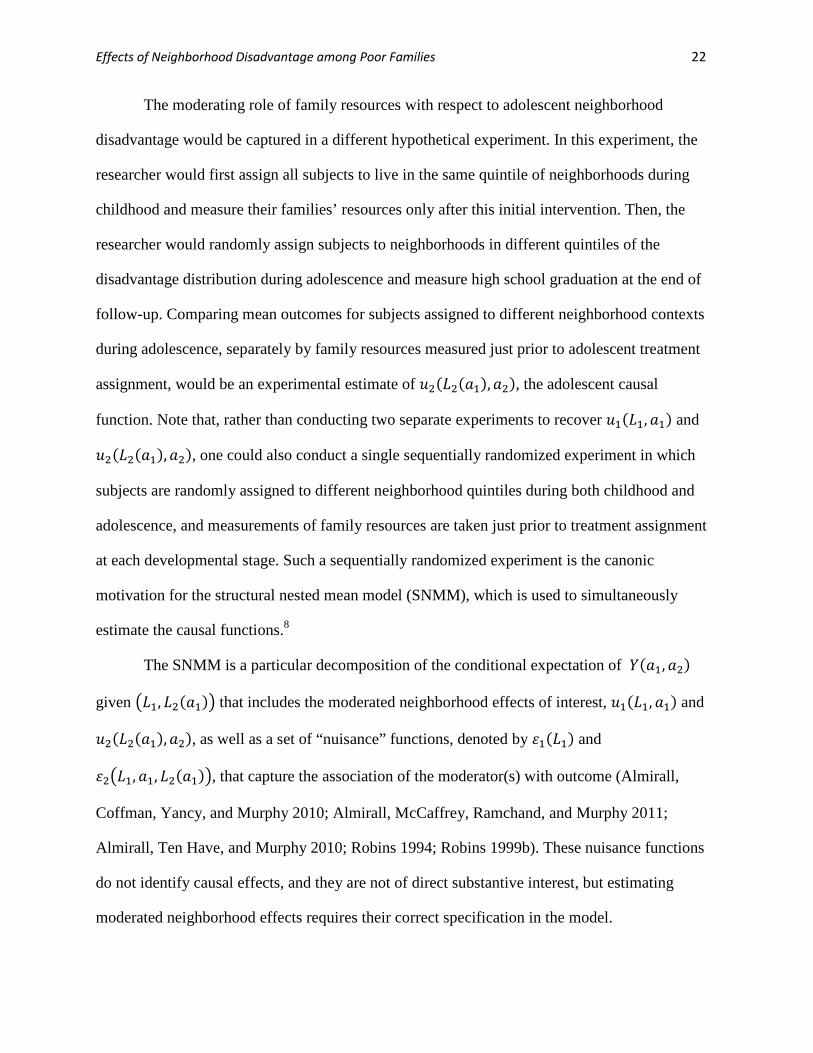
The moderating role of family resources with respect to adolescent neighborhood
disadvantage would be captured in a different hypothetical experiment. In this experiment, the
researcher would first assign all subjects to live in the same quintile of neighborhoods during
childhood and measure their families’ resources only after this initial intervention. Then, the
researcher would randomly assign subjects to neighborhoods in different quintiles of the
disadvantage distribution during adolescence and measure high school graduation at the end of
follow-up. Comparing mean outcomes for subjects assigned to different neighborhood contexts
during adolescence, separately by family resources measured just prior to adolescent treatment
assignment, would be an experimental estimate of 𝑢2(𝐿2(𝑎1),𝑎2), the adolescent causal
function. Note that, rather than conducting two separate experiments to recover 𝑢1(𝐿1,𝑎1) and
𝑢2(𝐿2(𝑎1),𝑎2), one could also conduct a single sequentially randomized experiment in which
subjects are randomly assigned to different neighborhood quintiles during both childhood and
adolescence, and measurements of family resources are taken just prior to treatment assignment
at each developmental stage. Such a sequentially randomized experiment is the canonic
motivation for the structural nested mean model (SNMM), which is used to simultaneously
estimate the causal functions.8
The SNMM is a particular decomposition of the conditional expectation of 𝑌(𝑎1,𝑎2)
given �𝐿1, 𝐿2(𝑎1)� that includes the moderated neighborhood effects of interest, 𝑢1(𝐿1,𝑎1) and
𝑢2(𝐿2(𝑎1),𝑎2), as well as a set of “nuisance” functions, denoted by 𝜀1(𝐿1) and
𝜀2�𝐿1,𝑎1, 𝐿2(𝑎1)�, that capture the association of the moderator(s) with outcome (Almirall,
Coffman, Yancy, and Murphy 2010; Almirall, McCaffrey, Ramchand, and Murphy 2011;
Almirall, Ten Have, and Murphy 2010; Robins 1994; Robins 1999b). These nuisance functions
do not identify causal effects, and they are not of direct substantive interest, but estimating
moderated neighborhood effects requires their correct specification in the model.
Effects of Neighborhood Disadvantage among Poor Families 23
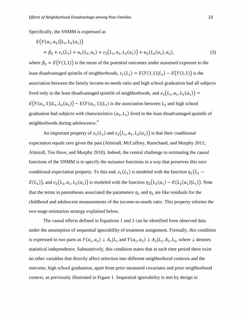
Specifically, the SNMM is expressed as
𝐸�𝑌(𝑎1,𝑎2)�𝐿1, 𝐿2(𝑎1)�
= 𝛽0 + 𝜀1(𝐿1) + 𝑢1(𝐿1,𝑎1) + 𝜀2�𝐿1,𝑎1, 𝐿2(𝑎1)� + 𝑢2(𝐿2(𝑎1),𝑎2), (3)
where 𝛽0 = 𝐸�𝑌(1,1)� is the mean of the potential outcomes under sustained exposure to the
least disadvantaged quintile of neighborhoods, 𝜀1(𝐿1) = 𝐸(𝑌(1,1)|𝐿1) − 𝐸�𝑌(1,1)� is the
association between the family income-to-needs ratio and high school graduation had all subjects
lived only in the least disadvantaged quintile of neighborhoods, and 𝜀2�𝐿1,𝑎1,𝐿2(𝑎1)� =
𝐸�𝑌(𝑎1, 1)|𝐿1, 𝐿2(𝑎1)� − 𝐸(𝑌(𝑎1, 1)|𝐿1) is the association between 𝐿2 and high school
graduation had subjects with characteristics (𝑎1,𝐿1) lived in the least disadvantaged quintile of
neighborhoods during adolescence.9
An important property of 𝜀1(𝐿1) and 𝜀2�𝐿1,𝑎1, 𝐿2(𝑎1)� is that their conditional
expectation equals zero given the past (Almirall, McCaffrey, Ramchand, and Murphy 2011;
Almirall, Ten Have, and Murphy 2010). Indeed, the central challenge to estimating the causal
functions of the SNMM is to specify the nuisance functions in a way that preserves this zero
conditional expectation property. To this end, 𝜀1(𝐿1) is modeled with the function 𝜂1�𝐿1 −
𝐸(𝐿1)�, and 𝜀2�𝐿1,𝑎1, 𝐿2(𝑎1)� is modeled with the function 𝜂2�𝐿2(𝑎1) − 𝐸(𝐿2(𝑎1)|𝐿1)�. Note
that the terms in parentheses associated the parameters 𝜂1 and 𝜂2 are like residuals for the
childhood and adolescent measurements of the income-to-needs ratio. This property informs the
two-stage estimation strategy explained below.
The causal effects defined in Equations 1 and 2 can be identified from observed data
under the assumption of sequential ignorability of treatment assignment. Formally, this condition
is expressed in two parts as 𝑌(𝑎1,𝑎2) ⊥ 𝐴1|𝐿1 and 𝑌(𝑎1,𝑎2) ⊥ 𝐴2|𝐿1,𝐴1, 𝐿2, where ⊥ denotes
statistical independence. Substantively, this condition states that at each time period there exist
no other variables that directly affect selection into different neighborhood contexts and the
outcome, high school graduation, apart from prior measured covariates and prior neighborhood
context, as previously illustrated in Figure 1. Sequential ignorability is met by design in
Effects of Neighborhood Disadvantage among Poor Families 24
experimental studies where treatment is randomly assigned at each time point. However, in
observational studies, such as the present investigation, satisfying this assumption requires data
on all the joint predictors of neighborhood disadvantage and high school graduation (we present
a sensitivity analysis for this assumption below).
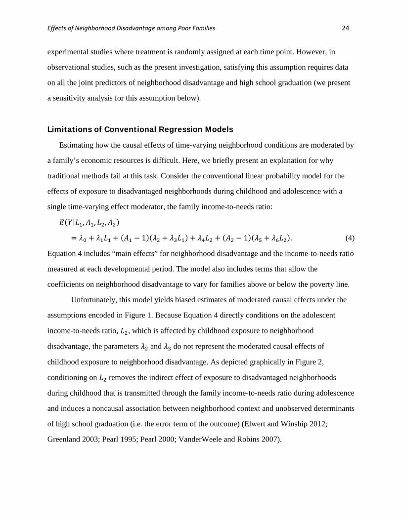
Limitations of Conventional Regression Models
Estimating how the causal effects of time-varying neighborhood conditions are moderated by
a family’s economic resources is difficult. Here, we briefly present an explanation for why
traditional methods fail at this task. Consider the conventional linear probability model for the
effects of exposure to disadvantaged neighborhoods during childhood and adolescence with a
single time-varying effect moderator, the family income-to-needs ratio:
𝐸(𝑌|𝐿1,𝐴1, 𝐿2,𝐴2)
= 𝜆0 + 𝜆1𝐿1 + (𝐴1 − 1)(𝜆2 + 𝜆3𝐿1) + 𝜆4𝐿2 + (𝐴2 − 1)(𝜆5 + 𝜆6𝐿2). (4)
Equation 4 includes “main effects” for neighborhood disadvantage and the income-to-needs ratio
measured at each developmental period. The model also includes terms that allow the
coefficients on neighborhood disadvantage to vary for families above or below the poverty line.
Unfortunately, this model yields biased estimates of moderated causal effects under the
assumptions encoded in Figure 1. Because Equation 4 directly conditions on the adolescent
income-to-needs ratio, 𝐿2, which is affected by childhood exposure to neighborhood
disadvantage, the parameters 𝜆2 and 𝜆3 do not represent the moderated causal effects of
childhood exposure to neighborhood disadvantage. As depicted graphically in Figure 2,
conditioning on 𝐿2 removes the indirect effect of exposure to disadvantaged neighborhoods
during childhood that is transmitted through the family income-to-needs ratio during adolescence
and induces a noncausal association between neighborhood context and unobserved determinants
of high school graduation (i.e. the error term of the outcome) (Elwert and Winship 2012;
Greenland 2003; Pearl 1995; Pearl 2000; VanderWeele and Robins 2007).

Effects of Neighborhood Disadvantage among Poor Families 25
With observational data in which time-varying moderators are affected by past levels of a
time-varying treatment, conventional regression models provide biased estimates of moderated
treatment effects even if there is no unobserved confounding of treatment (Robins 1987; Robins
1994; Robins 1999a). In other words, even with data from an optimal experiment that
sequentially randomized exposure to disadvantaged neighborhoods, conventional regression
models would fail to recover the moderated effects of neighborhood disadvantage if the
moderating covariates of interest were time-varying and affected by past neighborhood
conditions (Almirall, McCaffrey, Ramchand, and Murphy 2011; Almirall, Ten Have, and
Murphy 2010; Robins 1994; Robins 1999b). Thus, alternative methods are needed to estimate
moderated neighborhood effects in this study.10
Figure 2. Problems with conventional regression models
L1 L2
A1 A2
Y
U1
Notes: Ak = neighborhood disadvantage, Lk = family economic resources and other time-varying covariates, Uk = unobserved factors and Y = high school graduation. L1 includes time-invariant baseline covariates.
A. Over-control of intermediate pathways
L1 L2
A1 A2
Y
U1
B. Collider-stratification bias

Effects of Neighborhood Disadvantage among Poor Families 26
Two-stage Regression-with-Residuals Estimation
Almirall and colleagues (2011; 2010) provide a two-stage regression estimator for the
SNMM that is motivated by the zero conditional expectation property of the nuisance functions
discussed above. This approach is similar to estimating a conventional regression model, but it
proceeds in two steps. In the first stage, all time-varying covariates are regressed on the observed
past to obtain estimated residuals. For example, we regress the income-to-needs ratios in
childhood and adolescence on prior neighborhood context and time-varying covariates in models
with form 𝐸(𝐿1) = 𝛼0 and 𝐸(𝐿2|𝐿1,𝐴1) = 𝛾0 + 𝛾1𝐿1 + (𝐴1 − 1)(𝛾2 + 𝛾3𝐿1), and then we
estimate the residuals as 𝐿1𝑟 = 𝐿1 − 𝐸(𝐿1) and 𝐿2𝑟 = 𝐿2 − 𝐸(𝐿2|𝐿1,𝐴1). In the second stage, the
SNMM is estimated by regressing the observed outcome on neighborhood context and the
residualized time-varying covariates in a model with form,
𝐸(𝑌|𝐿1,𝐴1, 𝐿2,𝐴2)
= 𝛽0 + 𝜂1𝐿1𝑟 + (𝐴1 − 1)(𝛽1 + 𝛽2𝐿1) + 𝜂2𝐿2𝑟 + (𝐴2 − 1)(𝛽3 + 𝛽4𝐿2). (5)
As described above, the beta coefficients quantify how the probability of high school graduation
is expected to change with exposure to different neighborhood contexts during childhood versus
adolescence, conditional on prior income-to-needs, and the eta coefficients capture the
association between time-varying covariates and high school graduation. The only difference
between Equation 5 and the conventional regression model in Equation 4 is that Equation 5
includes “main effects” for the residualized time-varying covariates obtained from the first-stage
regressions rather than for the observed time-varying covariates. In other words, Equation 5 uses
𝜂1𝐿1𝑟 as the model for 𝜀1(𝐿1) and 𝜂2𝐿2𝑟 as the model for 𝜀2�𝐿1,𝑎1, 𝐿2(𝑎1)�, thereby satisfying the
zero conditional expectation property of the nuisance functions in the SNMM.
Figure 3 shows a stylized graph describing how the relationship between treatment and
future time-varying covariates changes after the latter are transformed into residuals.
Residualizing the adolescent income-to-needs ratio purges it of its association with neighborhood
disadvantage during childhood (i.e., no arrow from 𝐴1 to 𝐿2𝑟 ). Conditioning on the residualized
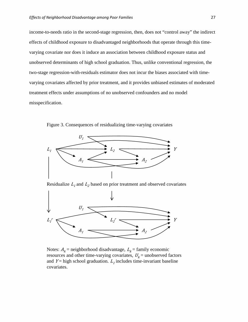
Effects of Neighborhood Disadvantage among Poor Families 27
income-to-needs ratio in the second-stage regression, then, does not “control away” the indirect
effects of childhood exposure to disadvantaged neighborhoods that operate through this time-
varying covariate nor does it induce an association between childhood exposure status and
unobserved determinants of high school graduation. Thus, unlike conventional regression, the
two-stage regression-with-residuals estimator does not incur the biases associated with time-
varying covariates affected by prior treatment, and it provides unbiased estimates of moderated
treatment effects under assumptions of no unobserved confounders and no model
misspecification.
Figure 3. Consequences of residualizing time-varying covariates
L1 L2
A1 A2
Y
U1
Notes: Ak = neighborhood disadvantage, Lk = family economic resources and other time-varying covariates, Uk = unobserved factors and Y = high school graduation. L1 includes time-invariant baseline covariates.
L1r L2
r
A1 A2
Y
U1
Residualize L1 and L2 based on prior treatment and observed covariates

Effects of Neighborhood Disadvantage among Poor Families 28
We compute two-stage regression estimates of the moderated effects of neighborhood
disadvantage on high school graduation, focusing on a single time-varying effect moderator, the
income-to-needs ratio, because theory suggests an important role for family economic resources
in buffering or amplifying the effects of neighborhood context. Other covariates are treated as
controls, entering only nuisance functions in the SNMM. Estimates are reported for the total
population and also for black and nonblack subjects separately in order to investigate potential
differences in the severity of neighborhood effects by race. Standard errors are estimated from
2,000 bootstrap samples (Efron and Tibshirani 1993).11
RESULTS
Sample Characteristics
Time-invariant covariates are summarized in Table 1, revealing considerable racial
inequalities. Overall, 80 percent of the total sample graduated high school by age 20, but only 75
percent of blacks are high school graduates compared to 85 percent of nonblacks. Parents of
black subjects are also much more disadvantaged than parents of nonblack subjects. For
example, blacks are more likely than nonblacks to have been born to young, unmarried mothers,
and black heads of household have much lower educational attainment than their nonblack
counterparts.
Table 1. Time-invariant covariates
Variable Total Blacks Nonblacks
% miss mean sd mean Sd mean sd S - high school graduate 43.0 .80 (.40) .75 (.44) .85 (.36) S - female 0.0 .48 (.50) .49 (.50) .48 (.50) M - age at childbirth 23.4 24.79 (5.56) 23.78 (5.62) 25.70 (5.35) M - married at childbirth 25.8 .71 (.45) .50 (.50) .90 (.30) H - high school graduate 2.9 .24 (.43) .25 (.43) .24 (.43) H - some college 2.9 .35 (.48) .22 (.41) .48 (.50) Notes: Results are combined estimates from 100 multiple imputation datasets. S, M and H indicate subject, mother of subject, and household head, respectively.

Effects of Neighborhood Disadvantage among Poor Families 29
Table 2 presents descriptive statistics for time-varying covariates, which further
document sizeable racial disparities. Nonblacks are much more likely than blacks to live with
heads of household that are married, employed, and who are homeowners. Nonblack families are
also smaller and less mobile than black families, and nonblacks have substantially more
economic resources at their disposal. Racial disparities in time-varying family covariates appear
to widen over time. For example, black-nonblack differences in marital and employment status,
as well as the income-to-needs ratio, increase between childhood and adolescence. Although the
economic position of both black and nonblack families improves over time, the improvement is
much greater for nonblacks, leading to growing racial disparities in material circumstances.
Table 2. Time-varying covariates
Variable Total Blacks Nonblacks
% miss mean sd mean Sd mean sd Childhood H - married 0.0 .73 (.40) .58 (.45) .87 (.29)
H - employed 0.0 .79 (.35) .67 (.40) .90 (.24)
FU - owns home 0.0 .46 (.45) .30 (.41) .61 (.44)
FU - size 0.0 4.85 (1.78) 5.23 (2.06) 4.51 (1.38)
FU - number of moves 13.1 1.15 (1.13) 1.20 (1.12) 1.11 (1.14)
FU - inc-to-needs ratio 0.0 .89 (1.22) .35 (.92) 1.37 (1.26) Adolescence H - married 23.8 .67 (.44)
.49 (.47)
.82 (.34)
H - employed 23.8 .78 (.37)
.65 (.42)
.89 (.25)
FU - owns home 23.8 .57 (.46)
.40 (.46)
.72 (.41)
FU - size 23.8 4.86 (1.57)
5.09 (1.83)
4.65 (1.25)
FU - number of moves 29.8 .76 (1.01)
.83 (1.03)
.69 (.98) FU - inc-to-needs ratio 23.8 1.28 (1.66) .55 (1.14) 1.95 (1.76) Notes: Results are combined estimates from 100 multiple imputation datasets. H and FU indicate household head and family unit, respectively.

Effects of Neighborhood Disadvantage among Poor Families 30
Neighborhood Conditions during Childhood and Adolescence
Table 3 describes exposure to different levels of neighborhood disadvantage during
childhood and adolescence for blacks and nonblacks. The main diagonal cells show the extent of
continuity in neighborhood conditions, while the off-diagonal cells describe upward and
downward neighborhood mobility.
Table 3. Joint treatment distribution n Blacks Nonblacks
row NH disadvantage quintile - adolescence NH disadvantage quintile - adolescence cell 1 2 3 4 5 1 2 3 4 5
NH
dis
adva
ntag
e qu
intil
e - c
hild
hood
1 38 11 6 8 5 358 49 23 15 3 .56 .16 .09 .12 .07 .80 .11 .05 .03 .01 .01 .00 .00 .00 .00 .11 .02 .01 .00 .00
2 19 26 28 12 6 169 279 87 31 6 .21 .29 .31 .13 .07 .30 .49 .15 .05 .01 .01 .01 .01 .00 .00 .05 .09 .03 .01 .00
3 20 37 62 39 38 48 245 356 107 34 .10 .19 .32 .20 .19 .06 .31 .45 .14 .04 .01 .01 .02 .01 .01 .01 .08 .11 .03 .01
4 15 24 75 180 152 34 61 229 425 130 .03 .05 .17 .40 .34 .04 .07 .26 .48 .15 .01 .01 .03 .06 .05 .01 .02 .07 .13 .04
5 14 33 76 239 1738 8 13 49 144 331 .01 .02 .04 .11 .83 .01 .02 .09 .26 .61 .00 .01 .03 .08 .60 .00 .00 .02 .04 .10
Notes: Results based on first imputation dataset.
Among blacks, 60 percent are exposed to the most disadvantaged quintile of American
neighborhoods during both childhood and adolescence. While the majority of blacks grow up in
highly disadvantaged neighborhoods, a nontrivial number live in less disadvantaged areas and
some of these individuals are upwardly mobile. For example, among blacks living in third
quintile neighborhoods during childhood, about 30 percent remain in these neighborhoods and
another 30 percent move to even less disadvantaged neighborhoods during adolescence.

Effects of Neighborhood Disadvantage among Poor Families 31
Downward neighborhood mobility is also common, however, with nearly 40 percent of
blacks in third quintile neighborhoods during childhood moving to more disadvantaged
neighborhoods in adolescence.
Compared to blacks, nonblacks grow up in much less disadvantaged neighborhoods.
Only 10 percent of nonblacks live in the most disadvantaged, fifth quintile of neighborhoods
throughout childhood and adolescence, and upward mobility from these areas is more common.
About 11 percent of nonblacks live in the least disadvantaged, first quintile of neighborhoods
throughout the early life course, and nearly 30 percent are continuously exposed to either first or
second quintile neighborhoods. By contrast, only about 3 percent of blacks live in either first or
second quintile neighborhoods during childhood and adolescence. Most nonblacks live in second
through fourth quintile neighborhoods during childhood, and many transition upward to less
disadvantaged neighborhoods in adolescence. The frequent mobility between different
neighborhood contexts among both blacks and nonblacks underscores the importance of
longitudinal measurement and dynamic modeling strategies in research on neighborhood effects.
Table 4 describes differences in exposure to neighborhood disadvantage during childhood
and adolescence by prior family resources. The rows in this table define different levels of the
income-to-needs ratio, where values below zero represent sub-poverty incomes and values
greater than zero represent incomes above the poverty line. Family resources during childhood
and adolescence are strongly related to neighborhood context, where those with higher income-
to-needs ratios are much less likely to live in the most disadvantaged neighborhoods and much
more likely to live in the least disadvantaged neighborhoods, compared to those with lower
income-to-needs ratios, as expected.
Poor families, however, are not restricted to living in disadvantaged neighborhoods, and
families of greater means are not bound to more advantaged communities. For example, Table 4
shows that 13 percent of families with income-to-needs ratios greater than two during childhood
(i.e., with incomes more than three times the poverty line) are exposed to the most disadvantaged
quintile of neighborhoods during the same developmental period. And among subjects in
families with incomes at or just above the poverty line during childhood, 4 percent and 8 percent
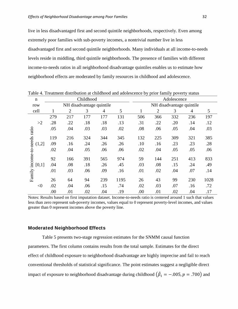
Effects of Neighborhood Disadvantage among Poor Families 32
live in less disadvantaged first and second quintile neighborhoods, respectively. Even among
extremely poor families with sub-poverty incomes, a nontrivial number live in less
disadvantaged first and second quintile neighborhoods. Many individuals at all income-to-needs
levels reside in middling, third quintile neighborhoods. The presence of families with different
income-to-needs ratios in all neighborhood disadvantage quintiles enables us to estimate how
neighborhood effects are moderated by family resources in childhood and adolescence.
Table 4. Treatment distribution at childhood and adolescence by prior family poverty status n Childhood Adolescence
row NH disadvantage quintile NH disadvantage quintile cell 1 2 3 4 5 1 2 3 4 5
Fam
ily in
com
e-to
-nee
ds ra
tio >2
279 217 177 177 131 506 366 332 236 197 .28 .22 .18 .18 .13 .31 .22 .20 .14 .12 .05 .04 .03 .03 .02 .08 .06 .05 .04 .03
(1,2] 119 216 324 344 345 132 225 309 321 385 .09 .16 .24 .26 .26 .10 .16 .23 .23 .28 .02 .04 .05 .06 .06 .02 .04 .05 .05 .06
[0,1] 92 166 391 565 974 59 144 251 413 833 .04 .08 .18 .26 .45 .03 .08 .15 .24 .49 .01 .03 .06 .09 .16 .01 .02 .04 .07 .14
<0 26 64 94 239 1195 26 43 99 230 1028 .02 .04 .06 .15 .74 .02 .03 .07 .16 .72 .00 .01 .02 .04 .19 .00 .01 .02 .04 .17
Notes: Results based on first imputation dataset. Income-to-needs ratio is centered around 1 such that values less than zero represent sub-poverty incomes, values equal to 0 represent poverty-level incomes, and values greater than 0 represent incomes above the poverty line.
Moderated Neighborhood Effects
Table 5 presents two-stage regression estimates for the SNMM causal function
parameters. The first column contains results from the total sample. Estimates for the direct
effect of childhood exposure to neighborhood disadvantage are highly imprecise and fail to reach
conventional thresholds of statistical significance. The point estimates suggest a negligible direct
impact of exposure to neighborhood disadvantage during childhood ��̂�1 = −.005, 𝑝 = .700� and

Effects of Neighborhood Disadvantage among Poor Families 33
provide no evidence of effect moderation by prior levels of the family income-to-needs ratio
��̂�2 = .005,𝑝 = .235�. For example, among individuals in poor families, even the most extreme
treatment contrast—exposure to the most disadvantaged quintile of neighborhoods during
childhood and then exposure to the least disadvantaged quintile of neighborhoods during
adolescence, compared to sustained residence in the least disadvantaged quintile of
neighborhoods—is estimated to reduce the probability of high school graduation by only 2
percentage points (i.e., 𝑢�1(𝐿1 = 0, 𝑎1 = 5) = 𝐸�(𝑌(5,1) − 𝑌(1,1)|𝐿1 = 0) = 4��̂�1 + �̂�2𝐿1� =
4�−.005 + .005(0)� = −.020, where 𝐿1 = 0 indicates that a subject’s family is at the poverty
line during childhood). Among individuals in families above or below the poverty line, the direct
effects of neighborhood disadvantage during childhood are also modest. Thus, regardless of
family resources, results indicate that childhood exposure to different neighborhood contexts has
a minimal impact on high school graduation if adolescent neighborhood conditions are held constant.
Table 5. Effects of neighborhood disadvantage on high school graduation (two-stage estimates)
Model Total Blacks Nonblacks
coef se coef Se coef se Intercept .888 (.021) *** .916 (.044) *** .877 (.019) *** Childhood NH dadvg –.005 (.012) –.004 (.019) –.006 (.015) NH dadvg x inc-to-needs .005 (.004) .005 (.008) .005 (.005) Adolesence NH dadvg –.042 (.010) *** –.054 (.018) ** –.026 (.013) †
NH dadvg x inc-to-needs .012 (.003) *** .017 (.006) ** .007 (.004) † Notes: Results are combined estimates from 100 multiple imputation datasets. Standard errors are based on 2000 bootstrap samples. †p < 0.10, *p < 0.05, **p < 0.01, and ***p < 0.001 for two-sided tests of no effect.
Estimates for the effect of adolescent neighborhood context, by contrast, indicate that
exposure to disadvantaged neighborhoods during this developmental period has a strong and
statistically significant negative effect on high school graduation ��̂�3 = −.042,𝑝 < .001� and
that this effect is substantially moderated by the family income-to-needs ratio ��̂�4 = .012,𝑝 <
.001�. Consistent with compound disadvantage theory, these estimates indicate that

Effects of Neighborhood Disadvantage among Poor Families 34
disadvantaged neighborhoods are especially harmful for individuals from poor families. For
example, among individuals in families living at the poverty line during adolescence, exposure to
the most disadvantaged quintile of neighborhoods, rather than the least disadvantaged quintile, is
estimated to reduce the probability of high school graduation by about 17 percentage points. For
individuals in families who are extremely poor during adolescence, exposure to the most
disadvantaged quintile of neighborhoods, compared to the least disadvantaged quintile, is
estimated to reduce the probability of high school graduation by nearly 20 percentage points (i.e.,
𝑢�2(𝐿2(𝑎1) = −.5,𝑎2 = 5) = 𝐸�(𝑌(𝑎1, 5) − 𝑌(𝑎1, 1)|𝐿2(𝑎1) = −.5) = 4��̂�3 + �̂�4𝐿2� =
4�−.042 + .012(−.5)� = −.192, where 𝐿2 = −.5 indicates that a subject’s family has an
income equal to one-half the poverty line during adolescence).
The effects of adolescent exposure to disadvantaged neighborhoods for nonpoor
individuals, on the other hand, are much less severe. Among individuals from nonpoor families
with incomes equivalent to three times the poverty line during adolescence, exposure to the most,
compared to the least, disadvantaged quintile of neighborhoods during the same developmental
period only reduces the probability of high school graduation by about 7 percentage points. In
sum, these results indicate that an individual’s chance of high school graduation is most sensitive
to neighborhood context during adolescence, and that family poverty intensifies the negative
effects of adolescent exposure to disadvantaged neighborhoods.
Separate effect estimates for blacks and nonblacks are reported in the second and third
columns of Table 5. These estimates are comparable to those from the total sample, indicating
that adolescent exposure to disadvantaged neighborhoods is highly consequential, while the
impact of exposure earlier during childhood is minimal, and that effects are most severe for
individuals living in poor families. Among blacks, exposure to the most disadvantage quintile of
neighborhoods during adolescence, compared to the least disadvantaged quintile, is estimated to
lower the probability of high school graduation by 25 percentage points for individuals whose
families are extremely poor, by about 21 percentage points for individuals in families at the
poverty line, and by only 8 percentage points for individuals in nonpoor families during
adolescence.

Effects of Neighborhood Disadvantage among Poor Families 35
Among nonblacks, estimates associated with adolescent neighborhood context are
smaller and only marginally significant, but they too suggest harmful effects for disadvantaged
neighborhoods during this developmental stage that are amplified by family resource
deprivation. Specifically, adolescent exposure to the most disadvantaged quintile of
neighborhoods, rather than the least disadvantaged quintile, is estimated to reduce the probability
of high school graduation by about 10 percentage points for nonblacks in poor families and by
about 5 percentage points for nonblacks in families with resources equivalent to three times the
poverty line.
Figure 4 displays probabilities of high school graduation for blacks with different
neighborhood and family resource histories computed from the SNMM estimates. The graph
shows how the probability of high school graduation would be expected to change if black
individuals that had lived in middle class, third quintile neighborhoods during childhood were
later exposed to different levels of neighborhood disadvantage in adolescence. Estimates are
plotted separately for subjects living in families that were extremely poor, poor, or nonpoor
during both childhood and adolescence to demonstrate the substantial magnitude of effect
moderation by the family income-to-needs ratio.
Results indicate that if blacks in both poor and extremely poor families had lived in third
quintile neighborhoods during childhood and then moved to a neighborhood in the least
disadvantaged quintile during adolescence, about 91 percent would have graduated high school
by age 20. If, on the other hand, these same individuals had moved from third quintile
neighborhoods in childhood to the most disadvantaged quintile of neighborhoods during
adolescence, only an estimated 69 percent of poor children and 65 percent of extremely poor
children would have graduated high school. For blacks living with nonpoor families, an
estimated 93 percent would have graduated had they moved, between childhood and
adolescence, from third quintile neighborhoods to neighborhoods in the least disadvantaged
quintile. About 86 percent of nonpoor blacks would be expected to graduate had they instead
moved to the most disadvantaged quintile of neighborhoods during adolescence.

Effects of Neighborhood Disadvantage among Poor Families 36
Notes: Childhood treatment set to residence in a third quintile, or middle class, neighborhood.
Figure 5 displays predicted probabilities of high school graduation for nonblacks by
neighborhood and family resource history. These estimates indicate that had nonblack
individuals in poor and in nonpoor families been exposed to third quintile neighborhoods during
childhood and then later moved to the least disadvantaged, first quintile of neighborhoods during
adolescence, about 87 percent of both groups would be expected to graduate from high school.
If, on the other hand, these individuals had moved to neighborhoods in the most disadvantaged
0.60
0.65
0.70
0.75
0.80
0.85
0.90
0.95
1 2 3 4 5
Pred
icte
d pr
obab
ility
of H
S gr
adua
tion
Neighborhood disadvantage quintile - adolescence
Extremely poor families
Poor families
Non-poor families
(least disadvantaged)
Figure 4. Predicted probability of high school graduation by adolescent exposure to neighborhood disadvantage and family poverty history, black respondents
(most disadvantaged)

Effects of Neighborhood Disadvantage among Poor Families 37
quintile during adolescence, only an estimated 77 percent of nonblacks in poor families and 83
percent of those in nonpoor families would have graduated high school.
Notes: Childhood treatment set to residence in a third quintile, or middle class, neighborhood.
Robustness Analyses
Under assumptions of no unobserved confounding (i.e., sequential ignorability) and no
model misspecification, the estimates presented above can be interpreted as average causal
effects of neighborhood context among different subgroups of children defined by their time-
0.60
0.65
0.70
0.75
0.80
0.85
0.90
0.95
1 2 3 4 5
Pred
icte
d pr
obab
ility
of H
S gr
adua
tion
Neighborhood disadvantage quintile - adolescence
Extremely poor families
Poor families
Non-poor families
(least disadvantaged)
Figure 5. Predicted probability of high school graduation by adolescent exposure to neighborhood disadvantage and family poverty history, nonblack respondents
(most disadvantaged)
Effects of Neighborhood Disadvantage among Poor Families 38
varying family resource history. These assumptions, although less stringent than those required
for conventional regression, are strong, and their violation would invalidate our inferences about
the moderated effects of disadvantaged neighborhoods. First, if either the causal or nuisance
functions of the SNMM were incorrectly specified, then our neighborhood-effect estimates
would be biased. Experimentation with a wide variety of specifications for both the causal and
nuisance functions, however, indicates that the reported estimates are quite robust (see Appendix B).
Second, if there are unmeasured factors that simultaneously affect neighborhood
selection and the probability of high school graduation, then our estimates are biased due to
unobserved confounding of neighborhood context. The assumption of no unobserved
confounding is not directly testable, but we measure and adjust for an extensive set of putative
confounders to mitigate this problem as much as possible. Furthermore, we investigate the
sensitivity of our effect estimates to hypothetical unobserved confounding. Results from this
formal sensitivity analysis, summarized in Appendix C, indicate that the magnitude of
unobserved confounding would have to be unreasonably large to alter our inferences about the
effects of adolescent exposure to disadvantaged neighborhoods. For example, among individuals
in poor families, we find that the effect of adolescent neighborhood disadvantage remains
statistically significant even in the extreme situation where unobserved confounding is assumed
to be twice as strong as the amount of confounding due to all observed covariates.
Finally, because some subjects drop out of the PSID before end of follow-up, a nontrivial
number are missing covariate and outcome data. To account for the uncertainty associated with
missing information, we report combined estimates from multiply imputed data. But in addition,
we also compute estimates using multiple imputation with deletion (von Hippel 2007), single
regression imputation (Longford 2005), and complete case analysis to investigate whether our
results are sensitive to different methods of missing data adjustment. Results indicate that
neighborhood effect estimates are stable under different procedures for handling missing data
(see Appendix D).
Effects of Neighborhood Disadvantage among Poor Families 39
DISCUSSION
Research on the spatial dimensions of social stratification is central to understanding the
reproduction of poverty and persistent educational inequality in America. Although the
educational consequences of disadvantaged neighborhoods are extensively studied, previous
research does not investigate whether neighborhood effects on high school graduation are
moderated by the evolving state of a child’s family environment or depend on the timing of
exposure to different neighborhood contexts during childhood versus adolescence. This study
integrates spatial, temporal, and developmental perspectives of the stratification process by
analyzing how the effects of different neighborhood contextual trajectories on high school
graduation are moderated by families’ economic resources in childhood and adolescence.
Using novel methods that properly account for dynamic neighborhood selection, this
study indicates that exposure to concentrated disadvantage, particularly during adolescence, has
a strong negative effect on the chances of high school graduation, and it reveals that the
consequences of adolescent exposure to disadvantaged neighborhoods are much more severe for
individuals whose families are also economically disadvantaged. By contrast, the effect of
neighborhood disadvantage is less pronounced among adolescents whose families live well
above poverty level. Neighborhood effects are thus moderated, time-dependent contextual
determinants of high school graduation.
Neighborhoods are important to “ecological” socialization models that describe how
interconnected social contexts influence child development (Brooks-Gunn, Duncan, Klebanov,
and Sealand 1993). This study demonstrates that such models must account for interactions
between nested contexts, like the family environment and neighborhood. Specifically, the
evidence presented in this study is consistent with the compound disadvantage theory of
neighborhood effect moderation, which contends that children in poor families are especially
vulnerable to the harmful effects of living in disadvantaged neighborhoods. Results indicate that
family resource deprivation greatly exacerbates the educational consequences of neighborhood

Effects of Neighborhood Disadvantage among Poor Families 40
deprivation. The “truly disadvantaged,” in this sense, are children simultaneously embedded in
impoverished families and impoverished neighborhoods, consistent with Wilson’s (1987)
seminal arguments about spatially concentrated poverty.
In addition to neighborhood effect moderation by family economic resources, this study
shows that it is essential to account for the longitudinal sequence of neighborhood contexts
experienced by individuals throughout the course of development. While previous research
documents the importance of duration of exposure to different neighborhood conditions
(Crowder and South 2010; Wodtke, Harding, and Elwert 2011), results presented here elaborate
these findings by demonstrating that neighborhood effects on high school graduation also depend
on the timing of exposure during childhood versus adolescence. Point estimates indicate that
exposure at both developmental periods reduces the probability of high school graduation, but
the effects of adolescent exposure are considerably larger and highly significant. These findings
add to the growing body of research indicating that neighborhood effects should be studied
within a longitudinal and developmental framework (Sampson, Sharkey, and Raudenbush 2008;
Sharkey and Elwert 2011; Wodtke, Harding, and Elwert 2011).
Investigating contextual effects within a temporal framework, however, requires new
methods that overcome critical problems with conventional regression analyses. Because time-
varying characteristics of the family environment are simultaneously mediators for the effect of
past neighborhood conditions and confounders for effect of future neighborhoods, conventional
regression estimators that condition on these covariates are biased due to over-control of
intermediate pathways and collider stratification. Several recent studies use inverse probability of
treatment weighting (Sampson, Sharkey, and Raudenbush 2008; Sharkey and Elwert 2011;
Wodtke, Harding, and Elwert 2011), a method that avoids the problems with conventional
regression, to estimate marginal, or population average, effects of neighborhood context. But
this approach is not designed for analyses of conditional, or moderated, neighborhood effects
among subgroups of children defined by time-varying family covariates. We use the SNMM and
Effects of Neighborhood Disadvantage among Poor Families 41
two-stage regression-with-residuals estimator (Almirall, McCaffrey, Ramchand, and Murphy
2011; Almirall, Ten Have, and Murphy 2010) to analyze neighborhood effect moderation by
family economic resources, a time-varying attribute that simultaneously confounds, mediates,
and moderates effects of past and future neighborhood exposures. The two-stage estimator is
unbiased for moderated neighborhood effects under a weaker set of assumptions than is required
for conventional regression, and analyses of potential violations of these assumptions indicate
that our results are robust. The methods used in this study can be easily adapted for time-varying
subgroup analyses of other contextual effects, such as the impact of school or firm
characteristics.
Although this study extends previous work on the temporal dimensions of neighborhood
effects, it is not without limitations. First, because the requisite data is unavailable for our sample
from the PSID, we are not able investigate the specific mechanisms, such as school quality or
environmental health hazards, through which structural neighborhood characteristics impact
children’s education progress. An important task for future research is to conduct mediation
analyses of neighborhood effects within an appropriate temporal framework. Second, this study
only examines a single educational outcome, high school graduation, measured during early
adulthood. Because of the timing of this particular school transition, our conclusions about the
importance of adolescent versus childhood exposure to disadvantaged neighborhoods should not
be extrapolated to other educational outcomes. Residence in disadvantaged neighborhoods
earlier rather than later in life likely has different consequences depending on the educational
outcome of interest. To better understand how neighborhood effects depend on timing of
exposure, future research should examine a variety of outcomes related to school progression and
achievement measured throughout the early life course.
These limitations notwithstanding, the present study provides important new evidence
about temporal dependency and family resource moderation of neighborhood effects on high
school graduation. With both income inequality and income segregation increasing in America
Effects of Neighborhood Disadvantage among Poor Families 42
(Reardon and Bischoff 2011), the devastating impact of spatially concentrated disadvantage on
high school graduation for children from poor families suggests that these broad social trends are
mutually reinforcing: income inequality begets income segregation, and income segregation
facilitates the reproduction of poverty.
END NOTES 1. Due to measurement limitations in the PSID, subjects with a general equivalency degree (GED) are coded as high school graduates. In addition, for subjects with item-specific missing data on educational attainment at age 20, we use measures of educational attainment taken at age 21, if available, to construct our indicator of high school graduation. 2. Classifying neighborhoods into quintiles of the composite disadvantage distribution results in some information loss about neighborhood context. Measurement error in treatment would be particularly concerning if it were linked to the moderating variable of interest, family poverty, because this might lead to inappropriate inferences about the degree of effect moderation. To investigate this issue, we also conduct analyses with the raw disadvantage index scores. Results (not reported) are very similar to those based on the quintile treatment definition. Because the quintile classification of neighborhoods greatly simplifies notation in the counterfactual model and facilitates a clean interpretation of effect estimates, we report results based on this treatment definition. 3. Parental education is treated as time-invariant because the PSID does not measure this factor at regular intervals, thereby limiting our ability to track changes over time. We use measurements of parental education taken when a child is age 2 or, if that is not available, the most recent measurement prior to age 2. 4. Some sample members leave the PSID before age 20 and thus are missing data for the outcome and covariates measured after their departure from the study. In addition to sample attrition, a small amount of data is missing due to item-specific nonresponse. Multiple imputation replaces missing data with 𝑚 > 1 values that are simulated from an imputation model. Separate estimates are computed for each of the 𝑚 complete datasets and then combined to account for the uncertainty associated with missing information. The combined estimates reported in this study are based on 𝑚 = 100 datasets. 5. In addition to reducing measurement error and accounting for duration of exposure, we measure neighborhood context and time-varying covariates using adjacent four-year averages to make the investigation of moderated neighborhood effects analytically tractable. Because the PSID provides annual measures of neighborhood context and time-varying covariates, we could, at least in theory, analyze the effects of different neighborhood exposures at every age during childhood and adolescence, conditional on family resource history through each time point. However, with separate annual measures, analyzing moderated neighborhood effects would require estimating millions of parameters, which is impossible with extant data. Thus, we divide the early life course into two developmental stages and measure key variables at each stage in a way that ensures unambiguous temporal ordering of the treatment, moderator, and confounders.

Effects of Neighborhood Disadvantage among Poor Families 43
6. When defining the moderated effects of neighborhood disadvantage during childhood, the analyst chooses the value to which adolescent treatment is set. We set adolescent treatment to residence in the least disadvantaged quintile of neighborhoods and define 𝑢1(𝐿1,𝑎1) as 𝐸(𝑌(𝑎1, 1) − 𝑌(1,1)|𝐿1) for two reasons. First, the resulting contrasts between childhood exposure sequences {(2,1), … , (5,1)} and sustained exposure to the least disadvantaged quintile of neighborhoods (1,1) are of key theoretical interest, and second, this formulation of 𝑢1(𝐿1,𝑎1) simplifies parameterization and interpretation of the causal function for adolescent neighborhood context. Note that different childhood treatment contrasts with, for example, adolescent treatment set to residence in a third quintile neighborhood, can be obtained from more complex combinations of model parameters. 7. Models that permit the effect of adolescent neighborhood disadvantage to be moderated by and the childhood measurements of neighborhood context and the income-to-needs ratio are also considered in supplemental analyses (see Table B.1 in Appendix B). There is no evidence that the effect of later exposure to disadvantaged neighborhoods during adolescence is moderated by neighborhood context or the family income-to-needs ratio measured earlier during childhood. Thus, we focus on the more parsimonious parameterization of adolescent neighborhood effects in Equation 2. 8. At this juncture, readers may wonder about other estimands that appear to represent moderated neighborhood effects but are not investigated in this study. For example, consider the question, “what is the effect of continuously living in the most disadvantaged quintile of neighborhoods, rather than the least disadvantaged quintile, among subjects whose families stay poor throughout the study?” This question, translated into counterfactual notation, is expressed as 𝐸�𝑌(5,5) − 𝑌(1,1)|𝐿1 = 0, 𝐿2 = 0)�. While this contrast may appear reasonable at first, it is not, in fact, a well-defined causal comparison: subjects whose families would stay poor had they continuously been exposed to the most disadvantaged neighborhoods and subjects whose families would stay poor had they been continuously exposed to the least disadvantaged neighborhoods are not the same set of individuals, and this comparison is therefore nonsensical because counterfactuals must compare the same subjects. Alternatively, consider the question, “what is the effect of continuously living in the most disadvantaged quintile of neighborhoods, rather than the least disadvantaged quintile, among subjects whose families would stay poor regardless of treatment received?” Translated into counterfactual notation, this question is expressed as 𝐸�𝑌(5,5)−𝑌(1,1)|𝐿1 = 0, 𝐿2(5) = 𝐿2(1) = 0)�. This is a well-defined causal contrast, but it cannot be identified because it is impossible to determine which families would stay poor regardless of treatment. Furthermore, it is unclear whether this effect is even a substantively interesting quantity, since it involves an unobservable subpopulation for which one of the mechanisms thought to mediate neighborhood effects is inoperative. By contrast, 𝑢1(𝐿1,𝑎1) and 𝑢2(𝐿2(𝑎1),𝑎2) are well-defined, identified under defensible assumptions, and substantively interesting in that they directly evaluate theories about compound disadvantage, relative deprivation, and developmental timing of neighborhood exposures. 9. Equation 3 is a parametric linear probability SNMM. The decomposition of the conditional mean on which the SNMM is based does not hold in nonlinear models, such as logit or probit regressions. While nonparametric linear probability, logit, and probit models are basically equivalent, parametric linear probability models can be problematic because they allow fitted values outside the logical [0,1] range. We find that this model provides a reasonable fit to the data without nonsensical predicted probabilities. In addition, models that relax the parametric restrictions in Equation 3 do not substantially alter the treatment-effect estimates of interest (see Appendix B). 10. In observational studies of neighborhood effects where time-varying confounders are affected by past neighborhood conditions, inverse probability of treatment (IPT) weighting can be used to estimate marginal, or population average, effects (Sampson, Sharkey, and Raudenbush 2008; Sharkey and Elwert 2011; Wodtke, Harding, and Elwert 2011). However, this approach precludes conditioning on time-

Effects of Neighborhood Disadvantage among Poor Families 44
varying covariates and thus does not permit analyses of moderated neighborhood effects when the moderator of interest varies across time, as in the present study. IPT weighting can be used to analyze effect moderation by baseline covariates only (Robins 1999b; Robins, Hernan, and Brumback 2000). 11. Bootstrapping is a method for estimating the variance of a sample statistic by resampling with replacement from the observed data. To compute bootstrap standard errors, we draw 𝑏 = 2,000 random samples of equal size to the observed data, apply the two-stage estimation procedure to each sample, and store the results. Then, the standard deviation of the 2,000 separate estimates obtained from this procedure gives the bootstrap estimate of the standard error. Hypothesis testing and p-values are based on a standard normal approximation.
REFERENCES
Aaronson, Daniel. 1998. "Using Sibling Data to Estimate the Impact of Neighborhoods on Children's Educational Outcomes." Journal of Human Resources 33:915-46.
Almirall, Daniel, Cynthia J. Coffman, William S. Yancy, and Susan A. Murphy. 2010. "Structurnal Nested Models." Pp. 231-61 in Analysis of Observational Health Care Data Using SAS, edited by D. Faries, A. C. Leon, J. M. Haro, and R. L. Obenchain. Cary, NC: SAS Institute.
Almirall, Daniel, Daniel F. McCaffrey, Rajeev Ramchand, and Susan A. Murphy. 2011. "Subgroups Analysis when Treatment and Moderators are Time-varying." Prevention Science (electronic publication ahead of print): http://dx.doi.org/10.1007/s11121-011-0208-7.
Almirall, Daniel, Thomas Ten Have, and Susan A. Murphy. 2010. "Structural Nested Mean Models for Assessing Time-Varying Effect Moderation." Biometrics 66:131-9.
Anderson, Elijah. 1999. Code of the Street: Decency, Violence, and the Moral Life of the Inner City. New York: Norton.
Brooks-Gunn, Jeanne, Greg J. Duncan, and J. Lawrence Aber. 1997. Neighborhood Poverty (Vol. 1): Context and Consequences for Children. New York: Russell Sage.
Brooks-Gunn, Jeanne, Greg J. Duncan, Pamela K. Klebanov, and Naomi Sealand. 1993. "Do Neighborhoods Influence Child and Adolescent Development?" American Journal of Sociology 99:353-95.
Brumback, Babette A., Miguel A. Hernan, Sebastien J. P. A. Haneuse, and James M. Robins. 2004. "Sensitivity Analyses for Unmeasured Confounding Assuming a Marginal Structural Model for Repeated Measures." Statistics in Medicine 23:749-67.
Carter, Prudence L. 2005. Keepin' It Real: School Success Beyond Black and White New York: Oxford University Press.
Charles, Camille Z. 2003. "The Dynamics of Racial Residential Segregation." Annual Review of Sociology 29:167-207.
Crane, Jonathan. 1991. "Effects of Neighbohoods on Dropping Out of School and Teenage Childbearing." Pp. 299-320 in The Urban Underclass, edited by C. Jencks and P. E. Peterson. Washington, D.C.: Brookings.
Effects of Neighborhood Disadvantage among Poor Families 45
Crosnoe, Robert. 2009. "Low-Income Students and the Socioeconomic Composition of Public High Schools." American Sociological Review 74:709-30.
Crowder, Kyle and Scott J. South. 2010. "Spatial and Temporal Dimensions of Neighborhood Effects on High School Graduation." Social Science Research 40:87-106.
Darling, Nancy and Laurence Steinberg. 1997. "Community Influences on Adolescent Achievement and Deviance." Pp. 120-31 in Neighborhood Poverty (Vol. 2): Policy Implications in Studying Neighborhoods, edited by J. Brooks-Gunn, G. J. Duncan, and J. L. Aber. New York: Russell Sage.
Duncan, Greg J. and Jeanne Brooks-Gunn. 1997. Consequences of Growing Up Poor. New York: Russell Sage.
Duncan, Greg J., W. Jean Yeung, Jeanne Brooks-Gunn, and Judith R. Smith. 1998. "How Much Does Childhood Poverty Affect the Life Chances of Children?" American Sociological Review 63:406-23.
Earls, Felton and Mary Carlson. 2001. "The Social Ecology of Child Health and Well-being." Annual Review of Public Health 22:143-66.
Efron, Bradley and Robert J. Tibshirani. 1993. An Introduction to the Bootstrap. New York: Chapman and Hall.
Elwert, Felix and Christopher Winship. 2010. "Effect Heterogeneity and Bias in Main-Effects-Only Regression Models." Pp. 327-36 in Probability and Causality: A Tribute to Judea Pearl, edited by R. Dechter, H. Geffner, and J. Y. Halpern. London: College Publications.
Elwert, Felix and Christopher Winship. 2012. "Endogenous Selection Bias." Unpublished Manuscript. University of Wisconsin-Madison.
Fernandez, Roberto M. and Celina Su. 2004. "Space in the Study of Labor Markets." Annual Review of Sociology 30:545-69.
Ginther, Donna, Robert Haveman, and Barbara Wolfe. 2000. "Neighborhood Attributes as Determinants of Children's Outcomes: How Robust are the Relationships?" Journal of Human Resources 35:603-42.
Gottschalk, Peter, Sara McLanahan, and Gary D. Sandefur. 1994. "The Dynamics and Intergenerational Transmission of Poverty and Welfare Participation." Pp. 85-108 in Confronting Poverty: Prescriptions for Change, edited by S. Danziger, G. D. Sandefur, and D. H. Weinberg.
Greenland, Sander. 2003. "Quantifying Biases in Causal Models: Classical Confounding vs Collider-stratification Bias." Epidemiology 14:300-6.
Harding, David J. 2003. "Counterfactual Models of Neighborhood Effects: The Effect of Neighborhood Poverty on Dropping Out and Teenage Pregnancy." American Journal of Sociology 109:676-719.
Harding, David J. 2007. "Cultural Context, Sexual Behavior, and Romantic Relationships in Disadvantaged Neighborhoods." American Sociological Review 72:341-64.
Harding, David J. 2009. "Collateral Consequences of Violence in Disadvantaged Neighborhoods." Social Forces 88:757-84.
Effects of Neighborhood Disadvantage among Poor Families 46
Harding, David J. 2010. Living the Drama: Community, Conflict, and Culture among Inner-City Boys. Chicago: University of Chicago Press.
Harding, David J. 2011. "Rethinking the Cultural Context of Schooling Decisions in Disadvantaged Neighborhoods: From Deviant Subculture to Cultural Heterogeneity." Sociology of Education 84:322-39.
Heckman, James J. 2006. "Skill Formation and the Economics of Investing in Disadvantaged Children." Science 312:1900-1.
Heckman, James J. and Alan B. Krueger. 2004. Inequality in America: What Role for Human Capital Policies? Boston, MA: The MIT Press.
Holland, Paul W. 1986. "Statistics and Causal Inference." Journal of the American Statistical Association 81:945-60.
Iceland, John and Melissa Scopilliti. 2008. "Immigrant Residential Segregation in US Metropolitan Areas, 1990-2000." Demography 45:79-94.
Jackson, Margot I. and Robert D. Mare. 2007. "Cross-Sectional and Longitudinal Measurements of Neighborhood Experience and Their Effects on Children." Social Science Research 36:590-610.
Jencks, Christopher and Susan E. Mayer. 1990. "The Social Consequences of Growing Up in a Poor Neighborhood." Pp. 111-86 in Inner-City Poverty in the United States, edited by L. E. Lynn and M. G. H. McGreary. Washington, D.C.: National Academy Press.
Kawachi, Ichiro and Lisa F. Berkman. 2003. "Neighborhoods and Health." New York: Oxford University Press.
Lareau, Annette. 2000. Home Advantage: Social Class and Parental Intervention in Elementary Education. New York: Rowan and Littlefield.
Longford, Nicholas T. 2005. "Single Imputation and Related Methods." Pp. 37-58 in Missing Data and Small-Area Estimation: Modern Analytical Equipment for the Survey Statistician, edited by S. Fienberg and W. van der Linden. New York: Springer.
Marsh, Herbert. 1987. "The Big Fish Little Pond Effect on Academic Self-Concept." Journal of Educational Psychology 79:280-95.
Massey, Douglas S. 2004. "Segregation and Stratification: A Biosocial Perspective." Du Bois Review 1:7-25.
Massey, Douglas S. and Nancy A. Denton. 1993. American Apartheid: Segregation and the Making of the Underclass. Cambridge, MA: Harvard University Press.
Mayer, Susan. 1997. What Money Can't Buy: The Effect of Parental Income on Children's Outcomes. Cambridge, MA: Harvard University.
Pearl, Judea. 1995. "Causal Diagrams for Empirical Research." Biometrika 82:669-710. Pearl, Judea. 2000. Causality: Models, Reasoning, and Inference. Cambridge: Cambridge
University Press. Quillian, Lincoln. 2003. "How Long Are Exposures to Poor Neighborhoods? The Long-Term
Dynamics of Entry and Exit from Poor Neighborhoods." Population Research and Policy Review 22:221-49.

Effects of Neighborhood Disadvantage among Poor Families 47
Reardon, Sean F. and Kendra Bischoff. 2011. "Income Inequality and Income Segregation." American Journal of Sociology 116:1092-153.
Robins, James M. 1987. "A New Approach to Causal Inference in Mortality Studies with a Sustained Exposure Period--Application to Control of the Healthy Worker Survivor Effect." Mathematical Modeling 7:1393-512.
Robins, James M. 1994. "Correcting for Noncompliance in Randomized Trials Using Structural Nested Mean Models." Communications in Statistics-Theory and Methods 23:2379-412.
Robins, James M. 1999a. "Association, Causation, and Marginal Structural Models." Synthese 121:151-79.
Robins, James M. 1999b. "Marginal Structural Models versus Structural Nested Models as Tools for Causal Inference." Pp. 95-134 in Statistical Models in Epidemiology, edited by E. Halloran. New York: Springer-Verlag.
Robins, James M., Miguel A. Hernan, and Babette A. Brumback. 2000. "Marginal Structural Models and Causal Inference in Epidemiology." Epidemiology 11:550-60.
Royston, Patrick. 2005. "Multiple Imputation of Missing Values: Update." The Stata Journal 5:1-14.
Rubin, Donald B. 1974. "Estimating Causal Effects of Treatments in Randomized and Nonrandomized Studies." Journal of Educational Psychology 66:688-701.
Rubin, Donald B. 1987. Multiple Imputation for Nonresponse in Surveys. New York: J. Wiley & Sons.
Rumberger, Russell W. 1987. "High-School Dropouts: A Review of Issues and Evidence." Review of Educational Research 57:101-21.
Sampson, Robert J. 2001. "How Do Communities Undergird or Undermine Human Development? Relevant Contexts and Social Mechanisms." Pp. 3-30 in Does It Take a Village? Community Effects on Children, Adolescents, and Families, edited by A. Booth and N. Crouter. Mahwah, N.J.: Erlbaum.
Sampson, Robert J., Jeffrey D. Morenoff, and Thomas Gannon-Rowley. 2002. "Assessing "Neighborhood Effects": Social Processes and New Directions in Research." Annual Review of Sociology 28:443-78.
Sampson, Robert J. and Patrick Sharkey. 2008. "Neighborhood Selection and the Social Reproduction of Concentrated Racial Inequality." Demography 45:1-29.
Sampson, Robert J., Patrick Sharkey, and Stephen W. Raudenbush. 2008. "Durable Effects of Concentrated Disadvantage on Verbal Ability among African-American Children." Proceedings of the National Academy of Sciences 105:845-52.
Sharkey, Patrick and Felix Elwert. 2011. "The Legacy of Disadvantage: Multigenerational Neighborhood Effects on Cognitive Ability." American Journal of Sociology 116:1934-81.
Small, Mario L. and Katherine Newman. 2001. "Urban Poverty After The Truly Disadvantaged: The Rediscovery of the Family, the Neighborhood, and Culture." Annual Review of Sociology 27:23-45.
South, Scott J. and Kyle D. Crowder. 1997a. "Escaping Distressed Neighborhoods: Individual, Community, and Metropolitan Influences." American Journal of Sociology 102:1040-84.

Effects of Neighborhood Disadvantage among Poor Families 48
South, Scott J. and Kyle D. Crowder. 1997b. "Residential Mobility Between Cities and Suburbs: Race, Suburbanization, and Back-to-the-City Moves." Demography 34:525-38.
South, Scott J. and Kyle D. Crowder. 1998a. "Avenues and Barriers to Residential Mobility among Single Mothers." Journal of Marriage and the Family 60:866-77.
South, Scott J. and Kyle D. Crowder. 1998b. "Housing Discrimination and Residential Mobility: Impacts for Blacks and Whites." Population Research and Policy Review 17:369-87.
South, Scott J. and Kyle D. Crowder. 1999. "Neighborhood Effects on Family Formation: Concentrated Poverty and Beyond." American Sociological Review 64:113-32.
South, Scott J. and Kyle D. Crowder. 2010. "Neighborhood Poverty and Nonmarital Fertility: Spatial and Temporal Dimensions." Journal of Marriage and Family 72:89-104.
South, Scott J. and Glenn D. Deane. 1993. "Race and Residential Mobility: Individual Determinants and Structural Constraints." Social Forces 72:147-67.
Speare, Alden and Frances K. Goldscheider. 1987. "Effects of Marital Status Change on Residential Mobility." Journal of Marriage and the Family 49:455-64.
Timberlake, Jeffrey M. 2007. "Racial and Ethnic Inequality in the Duration of Children’s Exposure to Neighborhood Poverty and Affluence." Social Problems 54:319-42.
VanderWeele, Tyler J. 2009. "On the Distinction between Interaction and Effect Modification." Epidemiology 20:863-71.
VanderWeele, Tyler J. and James M. Robins. 2007. "Directed Acyclic Graphs, Sufficient Causes and the Properties of Conditioning on a Common Effect." American Journal of Epidemiology 166:1096-104.
VanderWeele, Tyler J. and James M. Robins. 2009. "Minimal Sufficient Causation and Directed Acyclic Graphs." The Annals of Statistics 37:1437-65.
von Hippel, Paul T. 2007. "Regression with Missing Ys: An Improved Strategy for Analyzing Multiply Imputed Data." Sociological Methodology 37:83-117.
Wheaton, Blair and Philippa Clarke. 2003. "Space Meets Time: Integrating Temporal and Contextual Influences on Mental Health in Early Adulthood." American Sociological Review 68:680-706.
Wilson, William J. 1987. The Truly Disadvantaged: The Inner City, the Underclass, and Public Policy. Chicago: University of Chicago Press.
Wilson, William J. 1996. When Work Disappears: The World of the New Urban Poor. New York: Vintage Books.
Wodtke, Geoffrey T., David J. Harding, and Felix Elwert. 2011. "Neighborhood Effects in Temporal Perspective: The Impact of Long-term Exposure to Concentrated Disadvantage on High School Graduation." American Sociological Review 76:713-36.
Yinger, John. 1995. Closed Doors, Opportunities Lost: The Continuing Costs of Housing Discrimination. New York: Russell Sage.

Effects of Neighborhood Disadvantage among Poor Families 49 APPENDIX A. NEIGHBORHOOD DISADVANTAGE INDEX
Figure A.1. Neighborhood socioeconomic characteristics by disadvantage index quintile
3 4 57
12
24 5
8
19
4
79
14
29
1214
16
20
38
11
21
29
38
50
40
21
14
10
7
31
19
14
11
8
0
10
20
30
40
50
60
70
1 2 3 4 5
Perc
ent
Neighborhood disadvantage quintile
Percent unemployedPercent receiving welfarePercent povertyPercent female-headed householdsPercent without high school diplomaPercent college graduatesPercent mgr/prof workers
Table A.1 Principal component weights and correlations
Variable 1st PC
Weight Corr Percent poverty .408 .861 Percent unemployed .371 .783 Percent receiving welfare .412 .868 Percent female-headed households .337 .711 Percent without high school diploma .378 .798 Percent college graduates –.348 –.735 Percent mgr/prof workers –.385 –.812 Component variance 4.449 Proportion total variance explained .636
Notes: Principal component analysis based on correlation matrix. Analysis includes all tract-year observations from the 1970 to 2000 U.S. censuses.
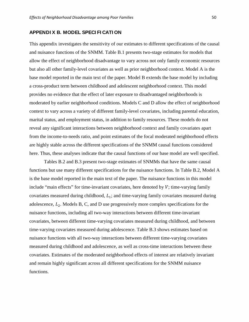
Effects of Neighborhood Disadvantage among Poor Families 50
APPENDIX B. MODEL SPECIFICATION
This appendix investigates the sensitivity of our estimates to different specifications of the causal
and nuisance functions of the SNMM. Table B.1 presents two-stage estimates for models that
allow the effect of neighborhood disadvantage to vary across not only family economic resources
but also all other family-level covariates as well as prior neighborhood context. Model A is the
base model reported in the main text of the paper. Model B extends the base model by including
a cross-product term between childhood and adolescent neighborhood context. This model
provides no evidence that the effect of later exposure to disadvantaged neighborhoods is
moderated by earlier neighborhood conditions. Models C and D allow the effect of neighborhood
context to vary across a variety of different family-level covariates, including parental education,
marital status, and employment status, in addition to family resources. These models do not
reveal any significant interactions between neighborhood context and family covariates apart
from the income-to-needs ratio, and point estimates of the focal moderated neighborhood effects
are highly stable across the different specifications of the SNMM causal functions considered
here. Thus, these analyses indicate that the causal functions of our base model are well specified.
Tables B.2 and B.3 present two-stage estimates of SNMMs that have the same causal
functions but use many different specifications for the nuisance functions. In Table B.2, Model A
is the base model reported in the main text of the paper. The nuisance functions in this model
include “main effects” for time-invariant covariates, here denoted by 𝑉; time-varying family
covariates measured during childhood, 𝐿1; and time-varying family covariates measured during
adolescence, 𝐿2. Models B, C, and D use progressively more complex specifications for the
nuisance functions, including all two-way interactions between different time-invariant
covariates, between different time-varying covariates measured during childhood, and between
time-varying covariates measured during adolescence. Table B.3 shows estimates based on
nuisance functions with all two-way interactions between different time-varying covariates
measured during childhood and adolescence, as well as cross-time interactions between these
covariates. Estimates of the moderated neighborhood effects of interest are relatively invariant
and remain highly significant across all different specifications for the SNMM nuisance
functions.
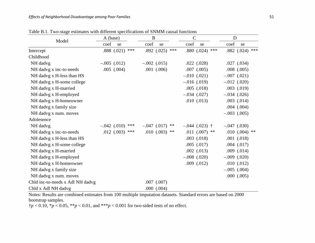
Effects of Neighborhood Disadvantage among Poor Families 51
Table B.1. Two-stage estimates with different specifications of SNMM causal functions
Model A (base) B C D coef se coef se coef se coef se
Intercept .888 (.021) *** .892 (.025) *** .880 (.024) *** .882 (.024) *** Childhood NH dadvg –.005 (.012) –.002 (.015) .022 (.028) .027 (.034) NH dadvg x inc-to-needs .005 (.004) .001 (.006) .007 (.005) .008 (.005) NH dadvg x H-less than HS –.010 (.021) –.007 (.021) NH dadvg x H-some college –.016 (.019) –.012 (.020) NH dadvg x H-married .005 (.018) .003 (.019) NH dadvg x H-employed –.034 (.027) –.034 (.026) NH dadvg x H-homeowner .010 (.013) .003 (.014) NH dadvg x family size .004 (.004) NH dadvg x num. moves –.003 (.005) Adolesence NH dadvg –.042 (.010) *** –.047 (.017) ** –.044 (.023) † –.047 (.030) NH dadvg x inc-to-needs .012 (.003) *** .010 (.003) ** .011 (.007) ** .010 (.004) **
NH dadvg x H-less than HS .003 (.018) .001 (.018) NH dadvg x H-some college .005 (.017) .004 (.017) NH dadvg x H-married .002 (.013) .009 (.014) NH dadvg x H-employed –.008 (.020) –.009 (.020) NH dadvg x H-homeowner .009 (.012) .010 (.012) NH dadvg x family size –.005 (.004) NH dadvg x num. moves .000 (.005) Chld inc-to-needs x Adl NH dadvg .007 (.007) Chld x Adl NH dadvg .000 (.004) Notes: Results are combined estimates from 100 multiple imputation datasets. Standard errors are based on 2000 bootstrap samples. †p < 0.10, *p < 0.05, **p < 0.01, and ***p < 0.001 for two-sided tests of no effect.

Effects of Neighborhood Disadvantage among Poor Families 52
Table B.2. Two-stage estimates with different specifications of SNMM nuisance functions
Model A (base) B C D coef se coef se coef se coef se
Intercept .888 (.021) .886 (.021) .879 (.021) .876 (.021) Childhood NH dadvg –.005 (.012) –.005 (.012) .000 (.012) –.005 (.012) NH dadvg x inc-to-needs .005 (.004) .006 (.004) .002 (.004) .005 (.004) Adolesence NH dadvg –.042 (.010) *** –.042 (.010) *** –.041 (.010) *** –.033 (.011) **
NH dadvg x inc-to-needs .012 (.003) *** .013 (.003) *** .012 (.003) *** .007 (.003) * Description Num. of 2nd stage parameters 25 39 69 99
Nuissance functions main effects for V, L1 and L2
A + all two-way interactions btw elements of V
B + all two-way interactions btw V and L1
C + all two-way interactions btw V and L2
Notes: Results are combined estimates from 100 multiple imputation datasets. Standard errors are based on 2000 bootstrap samples. For this analysis, V denotes time-invariant baseline characteristics. L1 and L2 denote time-varying factors measured during childhood and adolescence, respectively. †p < 0.10, *p < 0.05, **p < 0.01, and ***p < 0.001 for two-sided tests of no effect.
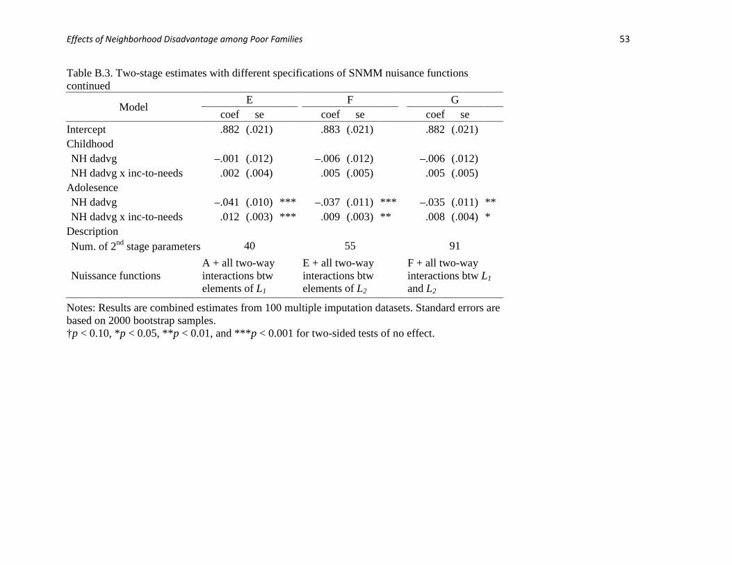
Effects of Neighborhood Disadvantage among Poor Families 53
Table B.3. Two-stage estimates with different specifications of SNMM nuisance functions continued
Model E F G
coef se coef se coef se Intercept .882 (.021) .883 (.021) .882 (.021) Childhood NH dadvg –.001 (.012) –.006 (.012) –.006 (.012) NH dadvg x inc-to-needs .002 (.004) .005 (.005) .005 (.005) Adolesence NH dadvg –.041 (.010) *** –.037 (.011) *** –.035 (.011) **
NH dadvg x inc-to-needs .012 (.003) *** .009 (.003) ** .008 (.004) * Description Num. of 2nd stage parameters 40 55 91
Nuissance functions A + all two-way interactions btw elements of L1
E + all two-way interactions btw elements of L2
F + all two-way interactions btw L1 and L2
Notes: Results are combined estimates from 100 multiple imputation datasets. Standard errors are based on 2000 bootstrap samples. †p < 0.10, *p < 0.05, **p < 0.01, and ***p < 0.001 for two-sided tests of no effect.

Effects of Neighborhood Disadvantage among Poor Families 54
APPENDIX C. SENSITIVITY ANALYSIS
In this section, we implement a formal sensitivity analysis to test the robustness of our estimates
to unobserved confounding, a violation of the sequential ignorability assumption. Unobserved
confounding would occur if families select different neighborhood contexts on the basis of
unmeasured factors that affect the chances of high school graduation. We consider unobserved
confounding of the following type: children currently living in more disadvantaged
neighborhoods may have lower graduation rates regardless of where they live, while children
currently living in less disadvantaged neighborhoods may have higher graduation rates
regardless of neighborhood context. This may occur because subjects living in disadvantaged
neighborhoods, compared to those living in more affluent communities, have parents that are less
“ambitious” or “skilled” when it comes to raising children or because they come from families
with less accumulated wealth. Since we lack reasonable measures of parental skill or ambition,
as well as family wealth, our neighborhood-effect estimates would be downwardly biased if
these characteristics are in fact confounders, indicating a negative impact of concentrated
disadvantage even if there is no such effect.
Following Sharkey and Elwert (2011), we implement a sensitivity analysis for time-
varying neighborhood treatments that models bias due to unobserved confounding as a function
of potential outcomes (Brumback, Hernan, Haneuse, and Robins 2004; Robins 1999a; Robins
1999b). With this approach, a selection function is used to summarize the relationship between
observed and counterfactual outcomes and then to compute bias-adjusted effect estimates. If
inferences about the negative effect of neighborhood disadvantage on high school graduation do
not change across a range of substantively reasonable confounding scenarios, as defined by
different values of the selection function, we conclude that our results are robust to unobserved
confounding.
To illustrate the logic behind this type of sensitivity analysis, consider a point-in-time
experiment that randomized a sample of families and their children to neighborhoods in each of
the five quintiles of the disadvantage distribution. Table C.1 provides a cross-tabulation of the
potential outcomes for this hypothetical experiment. The main diagonal cells give the observed
proportion of high school graduates in neighborhood quintile 𝑎 for subjects that were in fact
assigned to a neighborhood in quintile 𝐴 = 𝑎 of the composite disadvantage distribution. The
off-diagonal cells in parentheses are unobserved, or counterfactual, graduation rates. For
Effects of Neighborhood Disadvantage among Poor Families 55
example, cell (𝐸𝐸) is the graduation rate in the most disadvantaged quintile of neighborhoods
for individuals actually assigned to live in the least disadvantaged quintile of neighborhoods. In
an optimal randomized experiment, the potential outcome for a given treatment is the same for
members of all treatment groups, such that the observed and counterfactual graduation rates are
equal within columns: 𝐸 = (𝐹) = (𝐺) = (𝐻) = (𝐼), (𝐽) = 𝐾 = ⋯ = (𝑁), and so on. In other
words, with perfect randomization, the observed mean potential outcome among subjects living
in quintile 𝑎 should equal the unobserved mean potential outcome of living in quintile a among
subjects randomized to live in some other quintile 𝑎′. If the probability of high school graduation
is a linear function of neighborhood disadvantage, a regression of the observed outcome, 𝑌, on
the treatment variable, 𝐴, would provide a valid estimate of the average causal effect of
neighborhood disadvantage.
In this framework, unobserved confounding can be thought of as a departure from perfect
randomization of neighborhood context. Specifically, bias due to unobserved confounding occurs
if 𝐸 ≠ (𝐹) ≠ ⋯ ≠ (𝐼), (𝐽) ≠ 𝐾 ≠ ⋯ ≠ (𝑁), and so on. That is, if the observed mean outcome in
one treatment group is not exchangeable with the counterfactual mean outcome in the other
treatment groups, estimates are biased due to unobserved confounding. Based on this relationship
between observed mean outcomes and counterfactual mean outcomes, unobserved confounding
can be summarized by the following parsimonious selection function,
𝑠(𝑎,𝑎′) = 𝐸(𝑌(𝑎)|𝐴 = 𝑎) − 𝐸(𝑌(𝑎)|𝐴 = 𝑎′), (6)
where, for example, 𝑠(0,1) = 𝐸 − (𝐹). Different values of 𝑠(𝑎,𝑎′) correspond to varying types
and degrees of unobserved confounding.
For the present analysis, we adopt one particular specification of the selection function:
𝑠(𝑎,𝑎′) = (𝑎 − 𝑎′)𝛼, where 𝛼 ≤ 0 is a sensitivity parameter that specifies the magnitude of bias
due to unobserved confounding. We use a linear model for unmeasured confounding because our
empirical analysis of neighborhood effects is focused on estimating the parameters of a linear
SNMM. In this model, 𝛼 = 0 implies no unobserved confounding of neighborhood context, and
𝛼 < 0 defines the type of confounding described previously: children currently living in more
disadvantaged neighborhoods have lower graduation rates regardless of where they live, and
children currently living in less disadvantaged neighborhoods have higher graduation rates
regardless of neighborhood context. Note that this model constrains the magnitude of unobserved

Effects of Neighborhood Disadvantage among Poor Families 56
confounding to be the same across levels of observed covariates and moderators, that is, we
assume a uniform unobserved selection process for all subgroups in the analysis.
Based on this selection function, a bias-adjusted estimate for the average treatment effect
in the point-in-time context can be obtained from the following calculations. First, we compute
the proportion of subjects in each neighborhood quintile, denoted by 𝑃(𝐴) for 𝐴 = 1,2, … ,5.
Second, we subtract the bias term, 𝐵 = ∑ (𝐴 − 𝐴′)𝛼𝐴′=5𝐴′=1 𝑃(𝐴′), from the observed outcome, 𝑌, to
obtain a bias-adjusted outcome 𝑌𝑐 = 𝑌 − 𝐵. Finally, we estimate a bias-adjusted treatment effect
by regressing the corrected outcome, 𝑌𝑐, on the treatment variable, 𝐴. By selecting a range of
plausible values for the sensitivity parameter, 𝛼, and estimating bias-adjusted effects for each of
those values, we are able to assess the robustness of our results to different degrees of
unobserved confounding.
For the present analysis where treatment is time-varying, separate selection functions,
𝑠𝑘(𝑎𝑘,𝑎𝑘′ ), are used to model unobserved confounding in childhood (𝑘 = 1) and adolescence
(𝑘 = 2). The formula for the bias term is modified to account for the total bias accumulated
across developmental periods, 𝐵 = ∑ ∑ (𝐴𝑘 − 𝐴𝑘′ )𝛼𝑘𝐴𝑘′ =5
𝐴𝑘′ =1 𝑃(𝐴𝑘′ )𝑘=2
𝑘=1 , and then the adjusted
outcomes are computed as above. To incorporate effect moderation and controls for observed
confounders, we simply refit the SNMM using the adjusted outcomes, and this yields bias-
adjusted estimates for the impact of neighborhood disadvantage on high school graduation.
Following Sharkey and Elwert (2011), the sensitivity parameter, 𝛼𝑘, is calibrated such that a one
unit change corresponds to the amount of bias eliminated from our main effect estimates in the
childhood and adolescent causal functions after adjusting for all observed confounders. The
sensitivity of neighborhood effect estimates is thus interpreted in terms of multiples of observed
confounding bias.
Figures C.1 and C.2 display the results from this sensitivity analysis for the effects of
childhood and adolescent exposure to neighborhood disadvantage, respectively. In both figures,
separate bias-adjusted effect estimates are presented for children in poor and in nonpoor families.
The value of the sensitivity parameter, 𝛼, is plotted on the horizontal axis. A value of 𝛼 = 0
indicates no unobserved confounding and simply reproduces the estimates reported in Table 5.
For 𝛼 = −1, unobserved factors are assumed to confound the effect of neighborhood
disadvantage on high school graduation to the same extent as all observed covariates already

Effects of Neighborhood Disadvantage among Poor Families 57
controlled for in the regression, including race, parental education, marital status, employment
status, family structure, and so on. Because we adjust for a large and relevant set of observed
confounders, we judge values of 𝛼 < −1 to be implausible unobserved confounding scenarios.
The results of this sensitivity analysis indicate that our estimates and main substantive
conclusions are robust to unobserved confounding: across a wide range of values for 𝛼, we
conclude that the direct effect of exposure to disadvantaged neighborhoods during childhood is
small and not statistically significant for both poor and nonpoor children, while the effect of
adolescent neighborhood disadvantage is severe and remains statistically significant under a
moderate degree of unobserved confounding (𝛼 > −.5) for nonpoor children and under a high
degree of unobserved confounding (𝛼 > −1) for poor children. Even in the most extreme
situation where unobserved confounding is assumed to be twice as strong as that already
controlled for through observed covariates (𝛼 = −2), the negative effect of neighborhood
disadvantage on high school graduation among children in poor families remains substantively
large and statistically significant. Thus, based on the results in Figures C.1 and C.2, we conclude
that the neighborhood effect estimates presented in Table 5 are highly robust to unobserved
confounding.
Table C.1. Potential outcomes from hypothetical neighborhood experiment Observed Treatment
Mean Potential Outcome, 𝐸(𝑌(𝑎)|𝐴) 𝐸(𝑌(1)|𝐴) 𝐸(𝑌(2)|𝐴) 𝐸(𝑌(3)|𝐴) 𝐸(𝑌(4)|𝐴) 𝐸(𝑌(5)|𝐴)
𝐴 = 1 𝐸 (𝐽) (𝑂) (𝑇) (𝐸𝐸) 𝐴 = 2 (𝐹) 𝐾 (𝑃) (𝑈) (𝐹𝐹) 𝐴 = 3 (𝐺) (𝐿) 𝑄 (𝑉) (𝐺𝐺) 𝐴 = 4 (𝐻) (𝑀) (𝑅) 𝑊 (𝐻𝐻) 𝐴 = 5 (𝐼) (𝑁) (𝑆) (𝑋) 𝐼𝐼
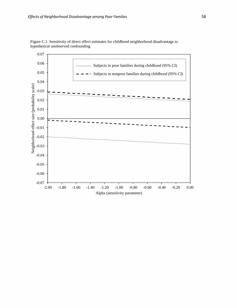
Effects of Neighborhood Disadvantage among Poor Families 58
-0.07
-0.06
-0.05
-0.04
-0.03
-0.02
-0.01
0.00
0.01
0.02
0.03
0.04
0.05
0.06
0.07
-2.00 -1.80 -1.60 -1.40 -1.20 -1.00 -0.80 -0.60 -0.40 -0.20 0.00
Nei
ghbo
rhoo
d ef
fect
size
(pro
babi
lity
scal
e)
Alpha (sensitivity parameter)
Figure C.1. Sensitivity of direct effect estimates for childhood neighborhood disadvantage to hypothetical unobserved confounding
Subjects in poor families during childhood (95% CI)
Subjects in nonpoor families during childhood (95% CI)
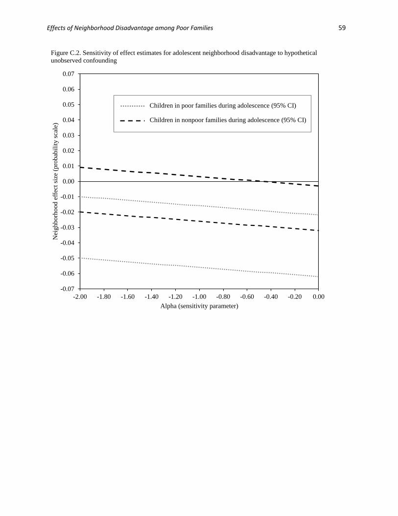
Effects of Neighborhood Disadvantage among Poor Families 59
-0.07
-0.06
-0.05
-0.04
-0.03
-0.02
-0.01
0.00
0.01
0.02
0.03
0.04
0.05
0.06
0.07
-2.00 -1.80 -1.60 -1.40 -1.20 -1.00 -0.80 -0.60 -0.40 -0.20 0.00
Nei
ghbo
rhoo
d ef
fect
size
(pro
babi
lity
scal
e)
Alpha (sensitivity parameter)
Figure C.2. Sensitivity of effect estimates for adolescent neighborhood disadvantage to hypothetical unobserved confounding
Children in poor families during adolescence (95% CI)
Children in nonpoor families during adolescence (95% CI)

Effects of Neighborhood Disadvantage among Poor Families 60
APPENDIX D. MISSING DATA ADJUSTMENTS
The analyses in this study suffer from a nontrivial amount missing data, summarized in Tables 1
and 2 of the main text, due primarily to attrition from the PSID. This appendix investigates
whether results change considerably using different methods of adjustment for missing data. The
first column of Table D.1 shows the combined estimates reported in the main text from 100
multiple imputation (MI) samples. Under the assumption that data are “missing at random”
(MAR), specifically, that conditional on observed covariates, the mechanism governing
missingness does not depend on unobserved factors that also affect the variable in question,
combined effect estimates and standard errors based on MI are unbiased and valid, respectively.
The second column contains combined estimates based on multiple imputation with deletion
(MID), a procedure where all missing data are multiply imputed but cases with missing values
for the outcome variable are deleted prior to estimation (von Hippel 2007). This approach offers
greater statistical efficiency than MI but requires more stringent assumptions about the missing
data mechanism. The third column contains estimates based on single regression imputation (SI)
for which missing values are replaced with the conditional sample mean. Under the MAR
assumption, this procedure yields unbiased effect estimates but understates their variance.
Finally, the last column presents estimates from a complete case analysis (CC) that simply
deletes all observations with any missing data. This procedure is unbiased only if data are
“missing completely at random” (MCAR), that is, only if the mechanism governing missingness
does not depend on observed or unobserved factors that affect the variable in question.
Combined estimates based on conventional MI are virtually identical to those obtained from
MID and are similar to those from SI and CC. We report MI estimates because this approach
requires the weakest assumptions for unbiased estimation and valid inference.
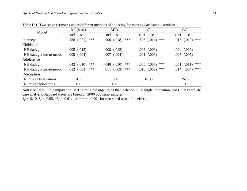
Effects of Neighborhood Disadvantage among Poor Families 61
Table D.1. Two-stage estimates under different methods of adjusting for missing data/sample attrition
Model MI (base) MID SI CC coef se coef se coef se coef se
Intercept .888 (.021) *** .906 (.018) *** .896 (.014) *** .915 (.019) *** Childhood NH dadvg –.005 (.012) –.008 (.012) .006 (.008) –.004 (.013) NH dadvg x inc-to-needs .005 (.004) .007 (.004) .001 (.003) .007 (.005) Adolesence NH dadvg –.042 (.010) *** –.040 (.010) *** –.055 (.007) *** –.051 (.011) ***
NH dadvg x inc-to-needs .012 (.003) *** .011 (.003) *** .016 (.002) *** .014 (.004) *** Description Num. of observations 6135 3500 6135 2626
Num. of replications 100 100 1 0 Notes: MI = multiple imputation, MID = multiple imputation then deletion, SI = single imputation, and CC = complete case analysis. Standard errors are based on 2000 bootstrap samples. †p < 0.10, *p < 0.05, **p < 0.01, and ***p < 0.001 for two-sided tests of no effect.