Polyphase-Coded FM (PCFM) Radar

Waveforms, Part II: Optimization

1Shannon D. Blunt, IEEE Senior Member,

1John Jakabosky, IEEE Student

Member, 2Matthew Cook, IEEE Member,

1James Stiles, IEEE Senior Member,

1Sarah Seguin, IEEE Member, and

3Eric L. Mokole, IEEE Fellow

This work was supported in part by the Centers of Excellence program of the Kansas Department of

Commerce, by the Radar Division of the US Naval Research Laboratory, through the Office of Naval

Research base funding program, and by the Air Force Office of Scientific Research. It was presented in

part at the 2011 and 2012 IEEE Radar Conferences [1,2].

1S.D. Blunt, J. Jakabosky, J. Stiles, and S. Seguin are with the Electrical Engineering & Computer Science

Dept., Radar Systems & Remote Sensing Lab, of the University of Kansas, Lawrence, KS. 2M. Cook is with the University of Kansas and Garmin International in Olathe, KS.

3E.L. Mokole is with the Radar Division of the US Naval Research Laboratory, Washington, DC.

2

Abstract

This paper addresses polyphase code optimization with respect to the nonlinear FM

waveform generated by the CPM implementation. A greedy search leveraging the complementary

metrics of PSL, ISL, and spectral content yield extremely low range sidelobes relative to

waveform time-bandwidth product. Transmitter distortion is also incorporated into the

optimization via modeling and actual hardware. Thus the physical radar emission can be

designed to address spectrum management and enable the physical realization of advanced

waveform-diverse schemes.

Keywords radar, pulse compression, continuous phase modulation, nonlinear distortion, radio spectrum

management, optimization methods, greedy algorithms

I. INTRODUCTION

The traditional approach to nonlinear FM (NLFM) waveform design relies on the

identification of a suitable continuous phase/frequency function of time (see Sect. 5.2 of

[3] for an overview). Many such methods are based on the principle of stationary phase

[4–6], which relates the power spectral density and the chirp rate at each frequency and

thereby shapes the spectral content of the waveform accordingly. Another class of NLFM

is hyperbolic FM (HFM), otherwise known as linear period modulation (LPM) [7,8].

Other design approaches include higher-order polynomials [9], use of the Zak transform

[10], and hybrid methods that also employ amplitude tapering on receive [11,12]. In this

paper, the authors explore the optimization of the class of NLFM waveforms denoted as

polyphase-coded FM (PCFM) that are made possible through the continuous phase

modulation (CPM) implementation.

In the companion paper [13], it was shown that the CPM implementation commonly

used for aeronautical telemetry, deep-space communications, and Bluetooth devices can

3

be modified to implement arbitrary polyphase radar codes as PCFM waveforms. With the

use of appropriate mismatch filtering on receive to compensate for increased range

sidelobes resulting from design mismatch, this scheme provides a means to use the large

existing library of polyphase codes on high-power radar systems. Furthermore, this new

code/waveform linkage provides the opportunity to optimize a code according to the

characteristics of the resulting continuous waveform, thereby ameliorating the design

mismatch problem. Such an approach can likewise be extended to incorporate the

distortion induced by the physical transmitter and thus facilitate actual physical emission

optimization.

The virtue of a coded structure is that its discrete nature allows for optimization of

the temporal signature through various code-search strategies [14–16]. Extension of this

discrete structure into the continuous domain via appropriate implementation [13] and

through the subsequent transmitter distortion thus provides a framework for optimizing

physical emissions by these same code-search strategies. Figure 1 illustrates this general

notion of emission optimization in which a candidate polyphase code is selected, is

implemented as a continuous PCFM waveform via CPM, and then is injected into the

transmitter where the waveform encounters spectral shaping and nonlinear effects.

Assessment of the resulting physical emission (a distorted version of the waveform) is

used to close the optimization loop and thereby drive the code-search process.

4

Figure 1: Notional representation of the optimization of physical radar emissions

Cast in the manner of Fig. 1 using the CPM implementation, the emission

optimization problem involves the determination of a sequence of N phase values (more

specifically, phase change values). If each of these N values can take on one of L possible

states, then there exist NL possible coded emissions (assuming, for operational time

scales, that the transmitter behavior is time invariant). For even modest values of N and L,

the computational requirements to search all possibilities quickly become intractable,

thus necessitating the search for adequate suboptimal solutions. Consequently, a variation

of the greedy code-search strategy known as Marginal Fisher’s Information (MFI) [16],

recently demonstrated as an effective means to search a high-dimensional solution space,

is employed. While the high dimensionality precludes the practical determination of a

globally optimal solution, it is shown that this greedy approach yields effective

suboptimal results, in part by leveraging a “performance diversity” concept that alternates

among multiple different, yet complementary, performance metrics. Also, for some

sensing applications, the argument can be made that many “good enough” emissions are

even preferable to a single “best” emission.

For emission optimization, three operational paradigms are considered: 1) an

idealized distortion-free transmitter; 2) transmitter distortion defined by a mathematical

5

model; and 3) incorporation of a physical transmitter. The distortion-free case is included

to demonstrate the potential of optimizing PCFM waveforms in this manner, with the

special classes of linear FM (LFM) [3, Sect. 4.2] and hyperbolic FM (HFM) [7,8]

waveforms used as benchmarks for comparison. Using mathematical models for

transmitter distortion [17] provides an efficient way to account for realistic transmitter

effects. This Model-in-the-Loop (MiLo) version of emission optimization may be useful

to determine the potential capabilities and deficiencies of various transmitter

components/topologies and may also serve as a starting point for inclusion of the physical

transmitter in the optimization process. Note that the efficacy of the MiLo approach is

clearly dependent upon how well the mathematical model reflects reality. Finally,

Hardware-in-the-Loop (HiLo) emission design involves the incorporation of a physical

transmitter into the optimization procedure. An L-band radar test bed at the University of

Kansas is used to demonstrate HiLo design.

The remainder of the paper is organized as follows. Section II establishes a formal

framework that connects the discrete code to the physical emission, thus facilitating

optimization. Section III discusses the code-search process used herein and the various

optimization criteria. In Section IV, the distortion-free case is considered, and optimized

PCFM waveforms are assessed according to standard benchmarks. Finally, the capability

to optimize physical emissions for MiLo and HiLo schemes is demonstrated (Section V).

II. CODIFYING THE EMISSION

As shown in Figure 1, the physical PCFM radar emission can be characterized by

three stages: 1) an underlying discrete code comprised of a sequence of phase values that

6

2) undergoes a transformation into a continuous signal followed by 3) a subsequent

transformation representing the distortion imparted by the transmitter. Per the

formulation in [13], let 0 1 2, , , , N represent the collection of 1N phase values

in a constant-envelope polyphase code. The set 1 2, , , N is thus the collection of

“shortest path” phase changes between the pairs of adjacent phase values (see (1) and (2)

in [13]). Noting that the initial phase 0 is arbitrary with regard to the set of N phase

changes, the structure of the code can be compactly represented as the length-N vector

1 2

T

N x . (1)

The continuous phase modulation (CPM) implementation of radar codes can be

expressed in a compact manner as the composite operator

CPM( ; )s t Tx x (2)

representing [13, Fig. 4] that generates the continuous-time PCFM waveform associated

with the particular phase-change code x. Likewise, the distortion imparted by the

transmitter onto the continuous waveform can be represented by the operation

Tx Tx CPM( ; ) ( ; )u t T s t T T x x x , (3)

which produces the physical emission launched from the radar. Finally, defining the

operation ( ; )u t x as the performance evaluation of the resulting emission according to

some desired characteristic(s) like peak sidelobe level (PSL), integrated sidelobe level

(ISL), spectral containment, etc., the design problem can thus be stated as:

“optimize ( ; )u t x by selecting the parameters in 1 2

T

N x ”

7

according to a specified criteria for (see Section III.D). Hence, the notional emission

generation and optimization framework of Fig. 1 can be illustrated from a mathematical

perspective as shown in Fig. 2.

Figure 2: Mathematical representation for the optimization of PCFM radar emissions

While it is beyond the scope of this present work to explore it in depth, the specific

nature of the transmission operator TTx plays an important role in the actual radar

emission. Here, as a proof of concept, a standard transmitter distortion model and a

specific hardware instantiation are considered. However, the myriad combinations of

transmitter components and design topologies [18], combined with physical effects such

as mutual coupling and calibration of antenna arrays [19–21], as well as emerging

operating modalities such as MIMO [22] and adaptive waveform design [15], all serve to

illustrate a rich research problem with regard to the modeling, design, and incorporation

of the effect of TTx. It is clear that significant advances will necessarily require a holistic

consideration of the signal processing (waveform generation and receive processing), the

systems engineering attributes/capabilities for the particular sensing modality, and the

physical electromagnetic (EM) effects at the given operating frequencies. Also note that,

for a physical system, there is a practical limit to how well the modeled TTx can actually

be known, thus promoting the concerted use of both MiLo and HiLo approaches.

8

III. SEARCHING FOR OPTIMALITY

Numerous approaches exist for searching the NL possible coded emissions (genetic

algorithms, simulated annealing, etc.) with varying degrees of speed and effectiveness. In

contrast to a traditional code-search effort, the computational burden of the present

problem is more onerous due to the generation of the physical emission via (2) and (3)

and the subsequent evaluation of ( ; )u t x . The following subsections outline the

general search strategy used herein, as well as some specific procedures to enhance and

accelerate the search. A multi-metric performance framework is also incorporated that

aids in the avoidance of inadequate locally optimal solutions.

A) Systematic Search for Optimized Emissions

The search strategy used here is a piecewise greedy approach whereby 1N

parameters in the phase-change vector x are held constant while the remaining parameter

is perturbed to each of the L possible phase-change values [16]. The particular perturbed

value (say the th ) of this thn parameter that provides the greatest improvement

according to the performance evaluation subsequently replaces the previous value for

the thn parameter, following which the process is repeated for a different parameter. If no

improvement is possible, the parameter value is unchanged.

The phase change parameter n was defined in [13] as

if

2 sgn if

n nn n

n n n

, (4)

where

1 n n n for 1, ,n N , (5)

9

sgn( ) is the signum operation, and n is the phase value of the thn chip in the length-

(N1) polyphase code. Because the search process involves a piecewise perturbation of

the code parameters, it is instructive to note that a search in space is different from a

search in space. For implementation convenience, the latter is considered.

To initialize the search process, an initial phase-change code is defined as

(0) (0) (0) (0)1 2

T

N x , (6)

which produces the continuous waveform (0) (0)CPM( ; )s t Tx x and the subsequent

physical emission (0) (0) (0)Tx Tx CPM( ; ) ( ; )u t T s t T T

x x x . Likewise, after the thi

perturbation stage, the phase-change code is

( ) ( ) ( ) ( )1 2

Ti i i i

N x , (7)

with associated waveform ( ) ( )CPM( ; )i is t Tx x and physical emission

( ) ( )Tx CPM( ; )i iu t T T

x x .

If the th( 1)i stage involves the perturbation of the thn phase-change parameter n ,

then (7) is modified by using (4) as

( 1) ( ) ( ) ( ) ( ) ( )1 1 , 1, , , , , ,

Ti i i i i i

n n n n n N

x (8)

for the L possible values of the perturbation ,n , which are equally spaced on ,

including 0 (no change). With the subsequent candidate emission resulting from (8) as a

function of ,n defined as

( 1) ( 1)Tx CPM( ; )i i

n nu t T T

x x , (9)

10

the optimal ˆ,n with index ˆ is thus determined by

( 1) ( )ˆ arg min ( ; ) ( ; )i inu t u t x x (10)

depending on the prescribed performance metric . Once the optimal perturbation value

ˆ,n is determined, then the associated ( 1)ˆ i

n

x becomes ( 1)ix . The process is then

repeated for one of the other N phase-change parameters to obtain ( 2)ix and so on until

the desired performance is attained for the physical emission.

B) Optimized Perturbation Ordering

In the search procedure just described, the ordering of perturbation of the phase-

change parameters was not considered. From the perspective of a greedy search

paradigm, it is appropriate to follow an ordering whereby the particular parameter being

perturbed is the one that yields the greatest performance improvement. However, since it

is not known a priori which parameter n can be perturbed to provide the greatest

improvement, it is necessary to consider the perturbation of each of the N parameters

separately and thereafter perform an a posteriori selection. Note that for the perturbation

of n for each 1, 2, ,n N , the other 1N parameters are held constant such that this

procedure involves N separate parallel searches for the thi perturbation stage. This

search process can be stated formally by extending (10) as

( 1) ( )ˆˆ, arg min min ( ; ) ( ; )i in

n

n u t u t x x (11)

such that replacing the particular ( )ˆi

n with ( )ˆˆ ˆ,

in n

yields the most improvement

in the given metric .

11

The “super-greedy” search in (11) involves an N-fold increase in computational cost

as compared to a pre-determined or random ordering of parameter perturbations. While

parallel processing could clearly be employed to compensate for this high computational

burden, a line search technique is presented to reduce the number of necessary

performance evaluations.

C) Line Search in Phase Space

As stated in Section III.A, the search process necessitates the completion of a

performance evaluation of each candidate emission as ( 1)( ; )inu t x for a discrete set of

perturbation values ,n for 1, 2, , L and a given index n . To avoid the brute force

approach of evaluating the emission for all L values of ,n on , , the well-known

Fibonacci line search [23], or some variation thereof, can be used to focus successively

onto the region(s) of ,n for which the greatest improvement is obtained via (10).

It is assumed that ( 1)( ; )inu t x is a continuous function of ,n on , for a

fixed n, though not necessarily convex. Hence, a coarse gridding of the interval ,

into J sections can be established so that a separate line search is performed on each

section, followed by a selection of the best result from among the J sections. The benefit

of such a search strategy is evidenced by noting the impact of doubling the number of

discrete phase-space values for ,n to 2L . In this case, the brute force approach

requires L additional performance evaluations, while the piecewise line search need only

require J additional evaluations, which can be a significant computational savings for

12

modest values of J. For example, the results in Section IV indicate that the piecewise line

search works well for J 4.

D) Emission Assessment

There are multiple assessment metrics for with which one could optimize

emission performance. Perhaps the most common metric is the peak sidelobe level (PSL)

[24], denoted PSL, and given by

PSL

( ,0)( , ) max

(0,0)

for m ,T , (12)

where

( , ) ( ; ) ( ; )

Tj t

t T

e u t u t dt

x x (13)

is the ambiguity function in terms of delay and Doppler frequency . The PSL metric

in (12) considers the zero-Doppler cut of (13), where the interval m m, corresponds

to the time (range) mainlobe and ,T T is the time support of ( ,0) due to finite

pulse length. The PSL metric indicates the largest degree of interference that one point

scatterer can cause to another at a different range offset.

Another important metric is ISL, the integrated sidelobe level (ISL) [24], which for

the zero-Doppler cut of the ambiguity function can be defined as

m

mISL

0

( ,0)

( , )

( ,0)

T

d

d

. (14)

13

The ISL metric is particularly useful for establishing the susceptibility to distributed

scattering such as clutter.

The metrics in (12) and (14) may also be expanded to encompass non-zero Doppler

by generalizing the mainlobe and sidelobe regions to correspond to the interior and

exterior, respectively, of a range-Doppler ellipse. From a practical standpoint, the range-

Doppler sidelobe region need only comprise a Doppler interval that depends on feasible

target velocities. Thus a Doppler-tolerant aspect may also be incorporated into these

metrics by defining a skewed range-Doppler mainlobe ellipse.

For code optimization approaches in the literature, PSL tends to be the most

common basis for design. In contrast, most techniques to design continuous NLFM

waveforms rely upon shaping of the waveform power spectral density [11] to mimic the

effects of amplitude tapering while maintaining the constraint of a constant envelope. In

that same vein, a spectrum-based metric that is posed in terms of the error with respect to

a frequency template is defined to assess such waveforms. To that end, let ( )W f be a

frequency weighting template (for example, a Gaussian window) that is scaled to have

energy commensurate to that of a constant modulus pulse of duration T. For the emission

frequency response ( ; )U f x , parameterized on the phase-change code x , a frequency

template error (FTE) metric FTE can be defined as

H

L

FTE

H L

1( ; ) ( ; ) ( )

qfp p

f

U f U f W f dff f

x x , (15)

where Lf and Hf demarcate the edges of the frequency interval of interest. The values p

and q define the degree of emphasis placed on different frequencies. For p = 1 and q = 2,

the metric in (15) defines a form of frequency-domain mean-square error (MSE). It is this

14

version that shall be applied later in the paper. Alternatively, p > 1 overly emphasizes

frequencies with higher power (in-band) and p < 1 overly emphasizes frequencies with

lower power (out-of-band). Since the desire is to vary the phase as a free parameter for

optimization, it is only the spectral envelope that is used in (15) for optimization. Also,

because the power spectral density (PSD) is the Fourier transform of the autocorrelation,

the PSD-based metric of (15) is complementary to metrics based on the ambiguity

function (13) such as PSL (12) and ISL (14) in terms of optimizing the matched filter

response of a waveform.

E) Performance Diversity

The metrics in the previous section provide different ways to assess the same

fundamental goal – minimizing the range (and perhaps also Doppler) sidelobes. From an

optimization perspective, these complementary metrics may be exploited to facilitate a

form of performance diversity since each metric realizes a different performance surface

with regard to the emission, especially with regard to the locations of local minima. In

other words, if one metric gets stuck in a local minimum, switching to a different yet

complementary metric may allow continued progress, with no further improvement

occurring only in the unlikely event that all metrics experience the same local minimum.

Note that while multi-objective optimization generally involves the balancing of different

conflicting metrics, the multi-metric approach described here involves complementary

metrics that provide different perspectives on the same criterion: lower range sidelobes.

With regard to waveform optimization consider the example of a phase transition

code x comprised of 64 ( N) elements. Figure 3 depicts the possible change in

performance metric (the difference portion of (10)) when a single element of x

15

(specifically, index 23n ) is varied over the interval [ , ] under the condition of an

ideal transmitter. Note that the three (ISL, PSL, FTE) minima occur at slightly different

phase transition values due to different underlying performance surfaces which,

compounded over multiple optimization stages, can subsequently produce quite different

waveforms at convergence. Furthermore, upon expanding to consider the best

perturbation index n̂ over the set of all 64 possible phase transitions via (11), Fig. 4

reveals that the three metrics lead to three quite different results: the PSL metric indicates

ˆ 51n is the best phase transition to perturb; while ISL and FTE metrics indicate ˆ 59n

and ˆ 61n , respectively.

Figure 3: Change in performance metric (for PSL, ISL, and FTE) as a function of different values

for phase transition n = 23

16

Figure 4: Best change in performance metric (for PSL, ISL, and FTE) as a function of transition

index n. The different metrics indicate that different transition indices are the best: PSL( n̂ = 51 ),

ISL( n̂ = 59 ), and FTE( n̂ = 61 )

Employing this performance diversity paradigm, it has been found that emission

optimization performance for all these complementary metrics can be significantly

improved when a policy is instituted whereby the particular assessment metric is varied

for different optimization stages. The nature of the policy is arbitrary and could involve,

for example, a fixed interval of permutation stages for each metric in turn or,

alternatively, an independent random selection of the metric for each stage. While global

optimality is still not guaranteed, this form of metric-varying optimization helps avoid

more of the local minima, since convergence would only halt if none of the metrics could

provide sufficient further improvement.

IV. DISTORTION-FREE OPTIMIZATION

To evaluate the efficacy of this new design approach in the context of existing

waveforms, first consider the case of an idealized transmitter with no distortion. To

assess the performance of optimized PCFM waveforms, comparisons are made with the

17

well-known LFM chirp and the linear period modulation (LPM) waveform (otherwise

known as hyperbolic FM, a class of NLFM [8]). For the same time-bandwidth product,

these waveforms provide benchmarks for range resolution (LFM) and PSL (LPM).

Specifically, because a reduction in range sidelobes corresponds to better spectral roll-

off, the result is degradation in range resolution compared to the LFM benchmark.

However, the PSL value for LFM is known to be quite high at −13.5 dB. In contrast,

LPM waveforms have a lower bound on PSL of [7]

LPM bound 10PSL 20log ( ) 3BT dB (16)

for time-bandwidth product BT, which establishes a useful benchmark for sensitivity.

For the idealized transmitter, no distortion occurs so Tx( ; ) ( ; ) ( ; )u t T s t s t x x x .

Consider optimizing this idealized PCFM emission for a phase-transition code x

comprised of 64 ( N) elements, where each individual value of can take on one of 64

( L) phase transitions drawn from a uniform sampling on the interval [ , ] and

indexed as 1,2, , L , where 1 corresponds to and L corresponds to

. Consequently, we may express the thn phase transition n with index n as

12

1

nn

L

(17)

for 1,2, ,n N . Here the CPM implementation employs the rectangular (RECT)

shaping filter [13] which, using (17), closely approximates an LFM waveform when

n n . The optimization process is initialized with this LFM coding and the

autocorrelation mainlobe for (12) and (14) is defined with m nullmin[ , 2.5 ]pT where

18

null is the distance from the mainlobe peak to the 1st null and 2.5 pT is used to bound the

mainlobe width, for pT the transition interval defined in [13].

According to the mainlobe bandwidth for PCFM waveforms as defined in [13, Sect.

3], it is straightforward to show that N provides an approximate upper limit on the time-

bandwidth product (based on the first spectral null). Hence, for 64N the bound from

(16) reveals a PSL lower limit of 39.1 dB for LPM waveforms [7].

Using the metrics for PSL (12), ISL (14), and FTE (15) separately, Fig. 5 shows the

autocorrelations of the resulting optimized waveforms. In each case, the search process

from (11) is applied until no further convergence is observable (that is, a local minimum

is reached). Also shown in Fig. 5 is the result obtained from the performance diversity

paradigm in which the search process from (11) is repeated using the metric ordering

{ISL, PSL, FTE, ISL, PSL, FTE, ISL, PSL, FTE, PSL}, where the converged local

minimum solution for the metric in each step serves as the initialization of the next step.

This ordering is arbitrary, with the cycling structure used to avoid a successive repeat of

the same metric which would have no benefit. A comparison of the four cases (ISL, PSL,

FTE, and performance diversity) reveals that performance diversity yields substantial

improvement in sidelobe levels relative to the three individual metrics.

19

Figure 5: Autocorrelation of the optimized ideal emissions using the PSL, ISL, and FTE metrics

individually and the performance diversity paradigm

Figure 6: Autocorrelation of the optimized ideal emissions using the PSL, ISL, and FTE metrics

individually and the performance diversity paradigm (mainlobe zoom-in)

Figure 6 illustrates the mainlobe width for the different waveforms relative to the

LFM waveform. Table 1 quantifies the resolution for 3 dB and 6 dB mainlobe widths

relative to that of the baseline LFM waveform and the final PSL, ISL, and FTE metrics

for the four optimized waveforms (ISL only, PSL only, FTE only, and performance

20

diversity). It is found that optimization according to PSL only yields the least

improvement over LFM for all three performance metrics (based on final PSL, ISL, and

FTE values). That said, PSL optimization experiences little range resolution degradation

relative to LFM. While a marked improvement is observed when using ISL or FTE

individually, the clear winner in terms of sidelobe reduction is when all three metrics are

used in the framework of performance diversity. In fact, the final PSL value of 40.2 dB

for performance diversity is 1.1 dB better than the 39.1 dB lower bound defined above

for LPM waveforms. The trade-off for such improvement is a ~30% degradation in range

resolution (mainlobe broadening) relative to LFM.

Table 1: Quantified performance for optimization of idealized emissions

Table 2 provides the indices employed by (17) to generate the resulting optimized

PCFM waveforms. It is interesting to consider the associated phase transition sequences

shown in Fig. 7 which represent the time-frequency behavior. Compared to the initial

linear phase transition sequence using n n and L N in (17) that closely

approximates LFM, the four optimized waveforms exhibit a seemingly random dithering

that actually serves to break up the coherency which otherwise produces higher sidelobes.

This dithering aside, careful examination shows that all four waveforms follow a roughly

sideways S-shaped path close to the linear trajectory that is akin to traditional NLFM [3,

Sect. 5.2]. Also, the PSL and FTE sequences have short-term wideband components that

21

are similar to the emissions of some species of bats (see Rhinolophidae and

Mormoopidae in [25]).

Table 2: Phase transition indices (vector x) for optimized ideal emissions based on (17)

Figure 7: Discrete phase transition sequence x of emissions optimized for PSL, ISL, and FTE

individually and using performance diversity.

In terms of unwrapped phase, the PCFM waveforms generated by the four x

sequences in Table 2 still approximate the parabolic shape associated with the LFM

phase progression (Fig. 8). Thus the Doppler tolerance property is also largely retained. A

close-up of the delay-Doppler ambiguity function for the performance diversity

optimized waveform is shown in Fig. 9. Where traditional NLFM waveforms possess

22

significant deviation from LFM at the ends of the pulse, which leads to additional ridges

near the main range-Doppler ridge, these ridges are rather small for the optimized PCFM

waveforms because the deviation from linear now takes the form of localized frequency

dithering (Fig. 7). For the performance diversity ambiguity function (Fig. 9), the largest

range-Doppler sidelobe value outside the main delay-Doppler ridge is −16.4 dB.

Figure 8: Continuous phase progression of emissions optimized for PSL, ISL, and FTE individually

and using performance diversity. Standard LFM is included for comparison.

Figure 9: Partial delay-Doppler ambiguity function of the emission optimized under the

performance diversity framework

23

V. OPTIMIZATION OF RADAR EMISSIONS

Now consider the impact of transmitter distortion and the use of transmitter-in-the-

loop optimization to compensate for distortion-induced sensitivity degradation. The

radar transmitter is comprised of multiple components (mixers, filters, amplifiers, etc.)

that contribute to the distortion of the waveform. The most prominent source of distortion

tends to be the power amplifier, which induces a nonlinear amplitude compression as a

result of being operated in saturation to achieve high power efficiency.

There are essentially two ways in which the transmitter may be incorporated into the

process of optimizing the radar emission: 1) a Model-in-the-Loop (MiLo) formulation

that employs a mathematical model of the transmitter; and 2) direct use of Hardware-in-

the-Loop (HiLo). The former can exploit the benefits of high-performance computing and

massive parallelization to search efficiently for an optimized emission. However, the

MiLo approach cannot account for all attributes of the transmitter and thus there is a limit

to the fidelity that it can provide. In contrast, the HiLo approach allows the emission to be

tuned precisely to the physical hardware, though the physical generation of candidate

emissions and their subsequent capture for performance evaluation can introduce

significant latency into the optimization process. Both approaches are considered in the

next two subsections.

A) MiLo Optimization

The simplest approach for transmitter MiLo optimization can be realized using an

IIR filter such as a Chebyshev filter followed by a mathematical model of the amplitude

compression of the power amplifier. The filter replicates the spectral shaping of the

physical system and provides more realistic rise and fall times for the pulse along with

24

the amplitude ripple and phase distortion of a physical system. The power amplifier

causes nonlinear distortion that compounds the filtering effects.

Extensive work exists on modeling power amplifier distortion. In this analysis, the

model of a solid-state amplifier from [17] is adopted as it approximates the physical

amplifier to be used in the subsequent hardware assessment. Note that greater distortion

can be expected for tube-based power amplifiers, which remain in widespread use.

Denoting ( ; )s t x as the filtered version of the waveform that is input to the power

amplifier, the model-based emission can be expressed as

( ; ) ( ; ) ( ; )u t G s t s tx x x , (18)

where the compression term G is

A r

G rr

(19)

and

1/ 2

2

0

1

bb

v rA r

v r

A

. (20)

In (20), v is the small-signal gain, 0A is the saturating amplitude at the amplifier output,

and b is an integer that controls the softness of transition from linear to nonlinear. For the

ensuing results the values 10v , 0 1A , and 3b are used.

Figure 10 shows (in blue) the autocorrelation of the performance diversity waveform

optimized for an ideal transmitter (from Sect. IV). Driving this waveform into the model

above introduces distortion that produces increased sidelobe levels (in red) in the amount

of 4.6 dB for the PSL metric and 2.8 dB for the ISL metric (interestingly, the FTE metric

25

does not change). Applying the performance diversity approach to now optimize the

model-distorted emission (black trace) provides 4.4 dB of lost sensitivity for the PSL

metric and 2.2 dB for the ISL metric. However, the FTE metric is now degraded by 2.1

dB. Table 3 quantifies the various metrics.

Figure 10: Emission autocorrelation for the ideal optimization (distortion-free) case, the modeled

transmitter distortion case, and transmitter Model-in-the-Loop (MiLo) optimization

Table 3: Quantified Performance for MiLo Optimization

B) HiLo Optimization

Direct incorporation of the physical transmitter into the optimization process

naturally accounts for the eccentricities of the hardware and thus can be expected to

provide the most accurate result. To demonstrate the efficacy of HiLo optimization, the

26

L-band (fc = 1.842 GHz) radar test bed depicted in Fig. 11 is used with the anechoic

chamber at the University of Kansas to perform free-space emission optimization that

includes antenna effects. Here a Class A power amplifier is used which, in an attempt to

mimic some of the distortion effects of a high-power amplifier, is driven well into

saturation. Specifically, the 1 dB compression point for the amplifier is 6 dBm, and the

input power driving the amplifier is 11 dBm (thus 5 dB into saturation).

Following the CPM implementation of a candidate code (performed digitally in

Matlab), the resulting PCFM waveform is converted to in-phase and quadrature-phase

(I/Q) components and is then loaded onto the arbitrary waveform generator (AWG). The

AWG drives the waveform into a single sideband (SSB) modulator that upconverts the

waveform to L-band. The upconverted waveform is passed through the saturated solid-

state power amplifier and a quad-ridge horn transmit antenna. The receive antenna is a

standard-gain horn. Following attenuation and downconversion in the receiver, the

subsequent baseband signal is sampled by the digitizer and passed back to a Matlab

program running on a laptop (Fig. 11), where the emission is assessed. Due to the

absence of receiver clipping it is assumed that any distortion induced within the receive

chain is negligible relative to that introduced by the transmitter.

The performance diversity emission, optimized under ideal conditions from Section

IV, is again used as the initialization. Due to buffering delays in the arbitrary waveform

generator and the digitizer, the HiLo operation on this test bed is much slower than what

could be achieved in the MiLo case in simulation. Thus, only the PSL metric from (12) is

used to drive emission optimization. In practice, a high-fidelity model of the system

27

could be employed to obtain an initialization via MiLo that should subsequently only

require fine tuning with HiLo optimization.

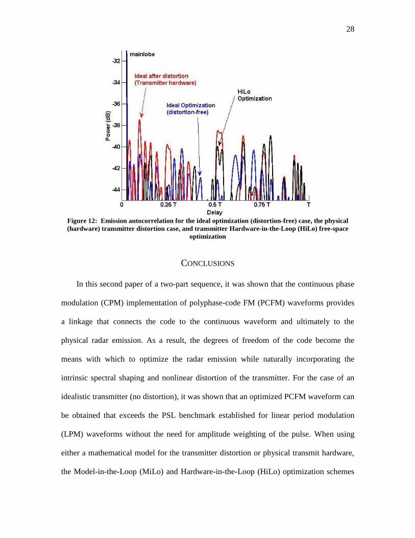
As expected, the transmitter hardware distorts the idealized emission (Fig. 12)

yielding 2.7 dB of PSL degradation. HiLo optimization is able to recover 1.5 dB of this

lost sensitivity. Table 4 quantifies the results according to the various metrics. Due to the

use of an available Class A power amplifier, the degree of degradation was rather limited.

Further studies are planned to investigate the amount of degradation and subsequent

performance recovery that can be obtained for high-power tube-based amplifiers.

Figure 11: L-band radar test bed (anechoic chamber in background)

Table 4: Quantified performance for HiLo Optimization

28

Figure 12: Emission autocorrelation for the ideal optimization (distortion-free) case, the physical

(hardware) transmitter distortion case, and transmitter Hardware-in-the-Loop (HiLo) free-space

optimization

CONCLUSIONS

In this second paper of a two-part sequence, it was shown that the continuous phase

modulation (CPM) implementation of polyphase-code FM (PCFM) waveforms provides

a linkage that connects the code to the continuous waveform and ultimately to the

physical radar emission. As a result, the degrees of freedom of the code become the

means with which to optimize the radar emission while naturally incorporating the

intrinsic spectral shaping and nonlinear distortion of the transmitter. For the case of an

idealistic transmitter (no distortion), it was shown that an optimized PCFM waveform can

be obtained that exceeds the PSL benchmark established for linear period modulation

(LPM) waveforms without the need for amplitude weighting of the pulse. When using

either a mathematical model for the transmitter distortion or physical transmit hardware,

the Model-in-the-Loop (MiLo) and Hardware-in-the-Loop (HiLo) optimization schemes

29

demonstrated the capability to recapture the lost sensitivity due to transmitter distortion.

This work sets the stage for the physical optimization of high-power radar emissions, the

design of emissions for exotic transmitter topologies proposed to enable better spectral

containment, and numerous new waveform diversity approaches.

REFERENCES

[1] J. Jakabosky, P. Anglin, M.R. Cook, S.D. Blunt, and J. Stiles, “Non-linear FM waveform

design using marginal Fisher’s information within the CPM framework,” IEEE Radar

Conf., pp. 513-518, Kansas City, MO, May 2011.

[2] J. Jakabosky, S.D. Blunt, M.R. Cook, J. Stiles, and S.A. Seguin, “Transmitter-in-the-loop

optimization of physical radar emissions,” IEEE Radar Conf., pp. 874-879, Atlanta, GA,

May 2012.

[3] N. Levanon and E. Mozeson, Radar Signals, John Wiley & Sons, Inc., Hoboken, NJ, 2004.

[4] E. Fowle, “The design of FM pulse compression signals,” IEEE Trans. Information Theory,

vol. 10, no. 1, pp. 61-67, Jan. 1964.

[5] C.E. Cook, “A class of nonlinear FM pulse compression signals,” Proceedings of the IEEE,

vol. 52, no. 11, pp. 1369-1371, Nov. 1964.

[6] R. De Buda, “Stationary phase approximations of FM spectra,” IEEE Trans. Information

Theory, vol. 12, no. 3, pp. 305-311, July 1966.

[7] T. Collins and P. Atkins, “Nonlinear frequency modulation chirps for active sonar,” IEE

Proc. Radar, Sonar & Navigation, vol. 146, no. 6, pp. 312-316, Dec. 1999.

[8] J.J. Kroszczynski, “Pulse compression by means of linear-period modulation,” Proc. IEEE,

vol. 57, no. 7, pp. 1260-1266, July 1969.

[9] A.W. Doerry, “Generating nonlinear FM chirp waveforms for radar,” Sandia Report,

SAND2006-5856, Sept. 2006.

[10] I. Gladkova, “Design of frequency modulated waveforms via the Zak transform,” IEEE

Trans. Aerospace & Electronic Systems, vol. 40, no. 1, pp. 355-359, Jan. 2004.

[11] J.A. Johnston and A.C. Fairhead, “Waveform design and Doppler sensitivity analysis for

nonlinear FM chirp pulses,” IEE Proc. F – Communications, Radar & Signal Processing,

vol. 133, no. 2, pp. 163-175, Apr. 1986.

[12] E. De Witte and H.D. Griffiths, “Improved ultra-low range sidelobe pulse compression

waveform design,” Electronics Letters, vol. 40, no. 22, pp. 1448-1450, Oct. 2004.

[13] S.D. Blunt, M. Cook, J. Jakabosky, J. de Graaf, E. Perrins, “Polyphase-coded FM (PCFM)

waveforms, part I: implementation,” to appear in IEEE Trans. AES.

[14] C.J. Nunn and G.E. Coxson, “Polyphase pulse compression codes with optimal peak and

integrated sidelobes,” IEEE Trans. Aerospace & Electronic Systems, vol. 45, no. 2, pp.

775-781, Apr. 2009.

[15] A. Nehorai, F. Gini, M.S. Greco, A.P. Suppappola, and M. Rangaswamy, Special Issue on

“Adaptive waveform design for agile sensing and communication,” IEEE Journal of

Selected Topics in Signal Processing, vol. 1, no. 1, June 2007.

[16] J.D. Jenshak and J.M. Stiles, “A fast method for designing optimal transmit codes for

radar,” IEEE Radar Conf., Rome, Italy, May 2008.

30

[17] E. Costa, M. Midrio, S. Pupolin, “Impact of amplifier nonlinearities on OFDM

transmission system performance,” IEEE Communications Letters, vol. 3, no. 2, pp. 37-39,

Feb. 1999.

[18] F.H. Raab, P. Asbeck, S. Cripps, P.B. Kenington, Z.B. Popovic, N. Pothecary, J.F. Sevic,

and N.O. Sokal, “Power amplifiers and transmitters for RF and microwave,” IEEE Trans.

Microwave Theory & Techniques, vol. 50, no. 3, Mar. 2002, pp. 814-826.

[19] C. Balanis, Antenna Theory, Wiley-Interscience, 2005, Sect. 8.7.

[20] S.D. Blunt, T. Chan, and K. Gerlach, “Robust DOA estimation: the reiterative

superresolution (RISR) algorithm,” IEEE Trans. Aerospace & Electronic Systems, vol. 47,

no. 1, pp. 332-346, Jan. 2011.

[21] B. Cordill, J. Metcalf, S.A. Seguin, D. Chatterjee, and S.D. Blunt, “The impace of mutual

coupling on MIMO radar emissions,” IEEE Intl. Conf. on Electromagnetics in Advanced

Applications, pp. 644-647, Torino, Italy, Sept. 2011.

[22] J. Li and P. Stoica, MIMO Radar Signal Processing, John Wiley & Sons, Inc., Hoboken,

NJ, 2009.

[23] D.A. Pierre, Optimization Theory with Applications, Dover Publications, 1986.

[24] M.A. Richards, J.A. Scheer, and W.A. Holm, Principle of Modern Radar: Basic Principles,

SciTech Publishing, 2010, pp. 793-794.

[25] M. Vespe, G. Jones, and C.J. Baker, “Lesson for radar: waveform diversity in echolocating

mammals,” IEEE Signal Processing Magazine, vol. 26, no. 1, pp. 65-75, Jan. 2009.