Polymorphism and Variant Analysis Lab Matt Hudson Polymorphism and Variant Analysis | Matt Hudson |...

Polymorphism and Variant Analysis | Matt Hudson | 2015

1

Polymorphism and Variant Analysis

Lab

Matt Hudson

PowerPoint by Casey Hanson


2

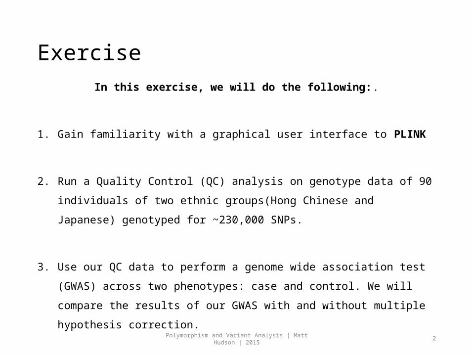
ExerciseIn this exercise, we will do the following:.

1. Gain familiarity with a graphical user interface to PLINK

2. Run a Quality Control (QC) analysis on genotype data of 90

individuals of two ethnic groups(Hong Chinese and Japanese)

genotyped for ~230,000 SNPs.

3. Use our QC data to perform a genome wide association test

(GWAS) across two phenotypes: case and control. We will compare

the results of our GWAS with and without multiple hypothesis

correction.


3

Step 0D: Local Files

For viewing and manipulating the files needed for this laboratory exercise, insert your flash drive.

Denote the path to the flash drive as the following:

[course_directory]

We will use the files found in:

[course_directory]/04_Variant_Analysis/data/


4

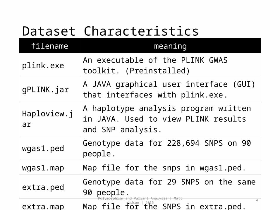
Dataset Characteristicsfilename meaning

plink.exeAn executable of the PLINK GWAS toolkit. (Preinstalled)

gPLINK.jarA JAVA graphical user interface (GUI) that interfaces with plink.exe.

Haploview.jarA haplotype analysis program written in JAVA. Used to view PLINK results and SNP analysis.

wgas1.pedGenotype data for 228,694 SNPS on 90 people.

wgas1.map Map file for the snps in wgas1.ped.

extra.pedGenotype data for 29 SNPS on the same 90 people.

extra.map Map file for the SNPS in extra.ped.

pop.covPopulation membership of the 90 people.(1 = Han Chinese, 2 = Japanese)


5

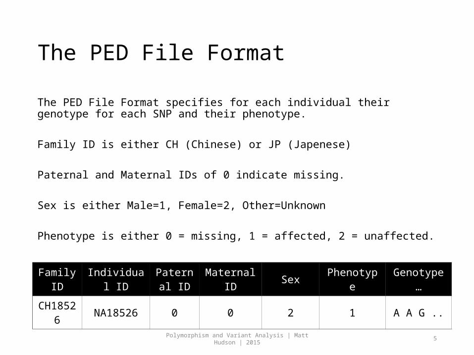
The PED File Format

The PED File Format specifies for each individual their genotype for each SNP and their phenotype.

Family ID is either CH (Chinese) or JP (Japenese)

Paternal and Maternal IDs of 0 indicate missing.

Sex is either Male=1, Female=2, Other=Unknown

Phenotype is either 0 = missing, 1 = affected, 2 = unaffected.

Family ID

Individual ID

Paternal ID

Maternal ID Sex Phenotype Genotype

…

CH18526 NA18526 0 0 2 1 A A G ..


6

The MAP File Format

The MAP File Format specifies the location of each SNP.

Note: Morgans (M) are a special kind of genetic distance derived from chromosomal recombination studies. Morgans can be used to reconstruct chromosomal maps.

chr SNP ID M Base Pair Position

8 rs17121574 12.8 12799052


7

Configuring gPLINKIn this exercise, we will configure gPLINK to work with our data.

Additionally, we will perform a format conversion to speed up our QC analysis.

Finally, we will validate our conversion and see what individuals and SNPs would be filtered out with default filters for QC analysis.


8

Step 1A: Starting gPLINK

gPLINK is a graphical user interface, written in JAVA, to the command line program PLINK.

To start gPLINK, navigate to

[course_directory]/04_Variant_Analysis/data/

Double click on gplink.jar.


9

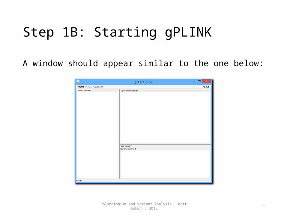
Step 1B: Starting gPLINK

A window should appear similar to the one below:


10

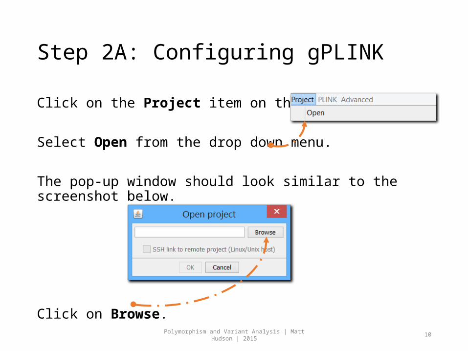
Step 2A: Configuring gPLINK

Click on the Project item on the Menu Bar.

Select Open from the drop down menu.

The pop-up window should look similar to the screenshot below.

Click on Browse.


11

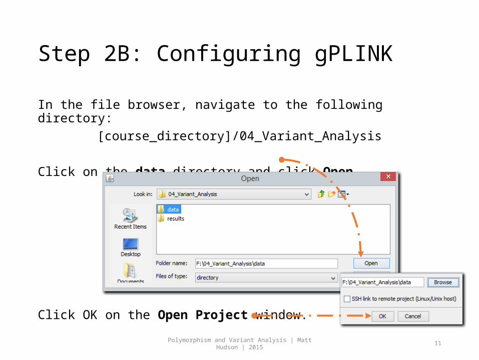
In the file browser, navigate to the following directory: [course_directory]/04_Variant_Analysis

Click on the data directory and click Open.

Click OK on the Open Project window.

Step 2B: Configuring gPLINK


12

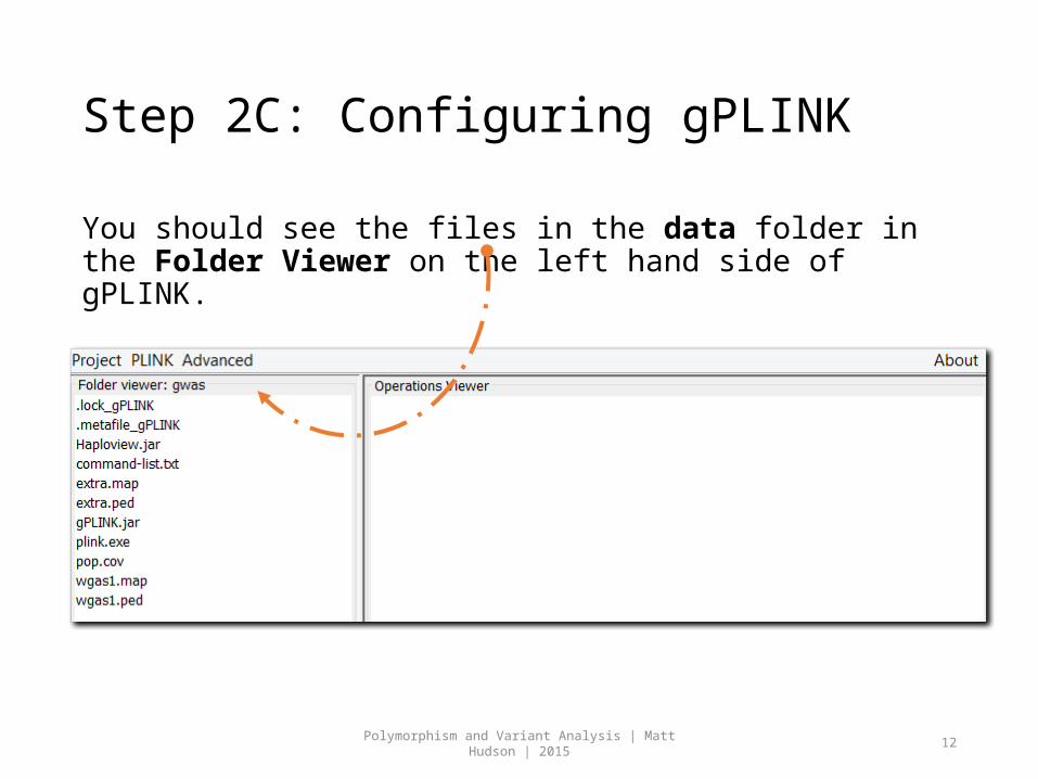
Step 2C: Configuring gPLINK

You should see the files in the data folder in the Folder Viewer on the left hand side of gPLINK.


13

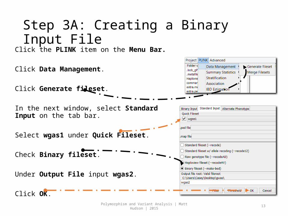
Step 3A: Creating a Binary Input File Click the PLINK item on the Menu Bar.

Click Data Management.

Click Generate fileset.

In the next window, select Standard Input on the tab bar.

Select wgas1 under Quick Fileset.

Check Binary fileset.

Under Output File input wgas2.

Click OK.


14

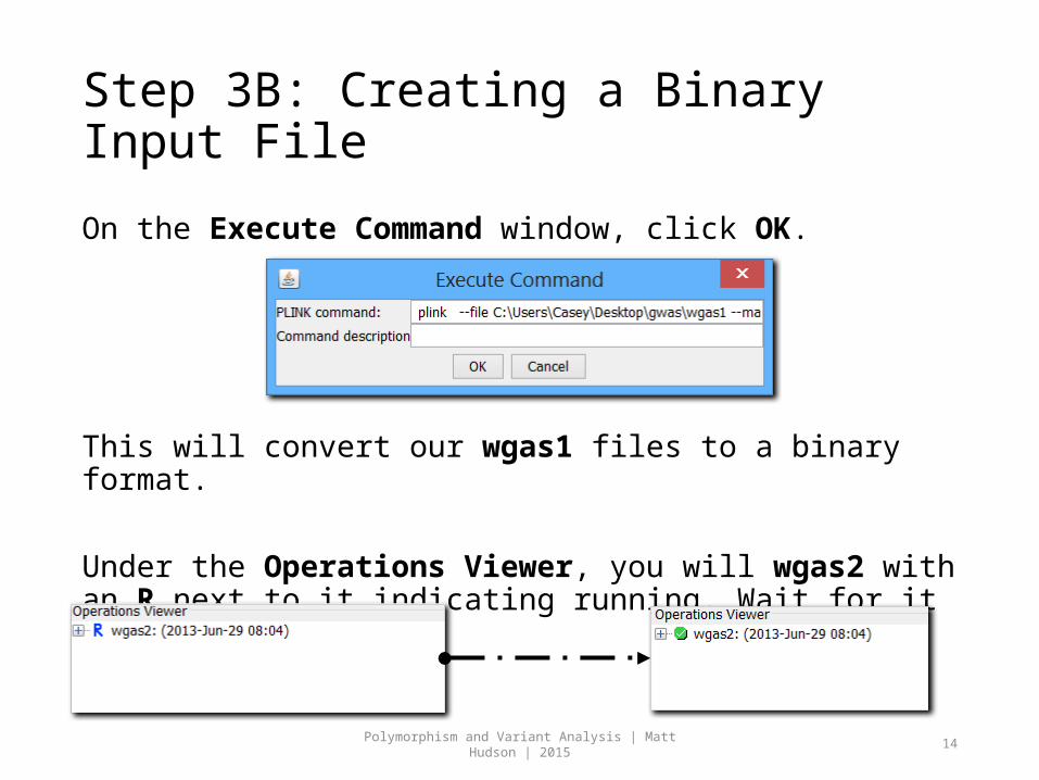
Step 3B: Creating a Binary Input File

On the Execute Command window, click OK.

This will convert our wgas1 files to a binary format.

Under the Operations Viewer, you will wgas2 with an R next to it indicating running. Wait for it to turn GREEN.


15

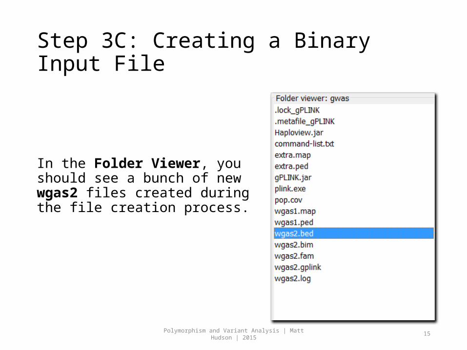
Step 3C: Creating a Binary Input File

In the Folder Viewer, you should see a bunch of new wgas2 files created during the file creation process.


16

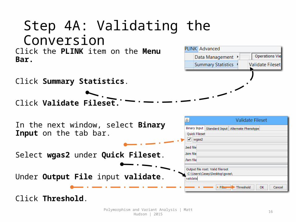
Step 4A: Validating the ConversionClick the PLINK item on the Menu Bar.

Click Summary Statistics.

Click Validate Fileset.

In the next window, select Binary Input on the tab bar.


Under Output File input validate.

Click Threshold.


17

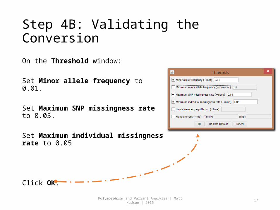
Step 4B: Validating the Conversion

On the Threshold window:

Set Minor allele frequency to 0.01.

Set Maximum SNP missingness rate to 0.05.

Set Maximum individual missingness rate to 0.05

Click OK.


18

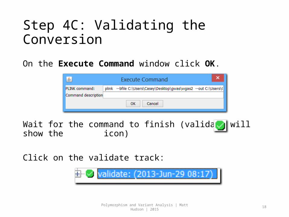
Step 4C: Validating the Conversion

On the Execute Command window click OK.

Wait for the command to finish (validate will show the icon)

Click on the validate track:


19

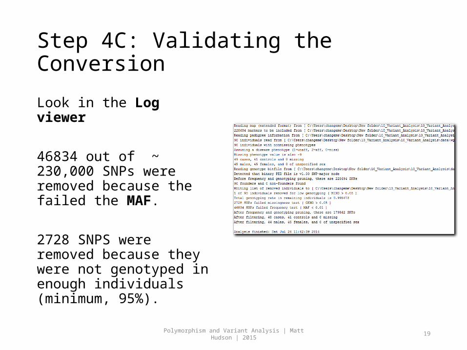
Step 4C: Validating the Conversion

Look in the Log viewer

46834 out of ~ 230,000 SNPs were removed because the failed the MAF.

2728 SNPS were removed because they were not genotyped in enough individuals (minimum, 95%).


20

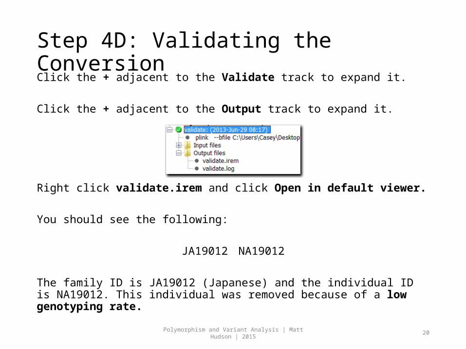
Step 4D: Validating the ConversionClick the + adjacent to the Validate track to expand it.

Click the + adjacent to the Output track to expand it.

Right click validate.irem and click Open in default viewer.

You should see the following:

JA19012 NA19012

The family ID is JA19012 (Japanese) and the individual ID is NA19012. This individual was removed because of a low genotyping rate.


21

Quality Control AnalysisIn this exercise, we will perform Quality Control Analysis (QC) to filter our data according to a set of criteria.


22

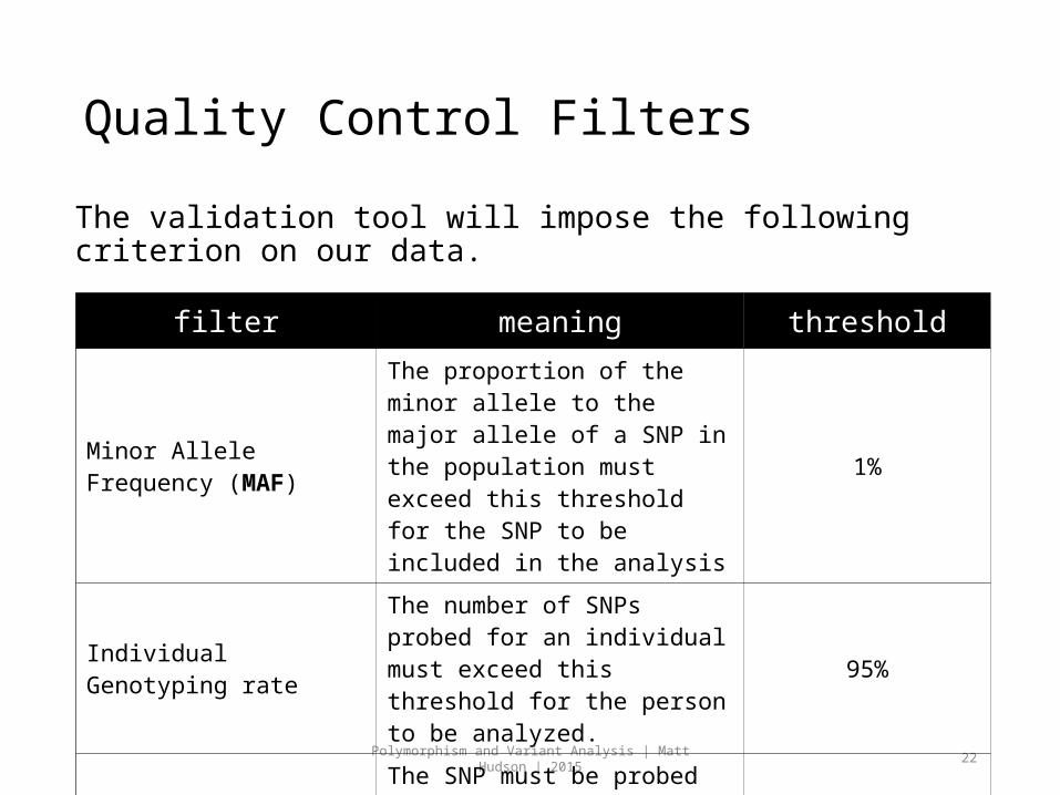
Quality Control Filters

The validation tool will impose the following criterion on our data.

filter meaning threshold

Minor Allele Frequency (MAF)

The proportion of the minor allele to the major allele of a SNP in the population must exceed this threshold for the SNP to be included in the analysis

1%

Individual Genotyping rate

The number of SNPs probed for an individual must exceed this threshold for the person to be analyzed.

95%

SNP genotyping rateThe SNP must be probed for at least this many individuals.

95%


23

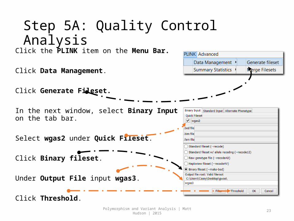
Step 5A: Quality Control AnalysisClick the PLINK item on the Menu Bar.

Click Data Management.

Click Generate Fileset.



Click Binary fileset.

Under Output File input wgas3.

Click Threshold.


24

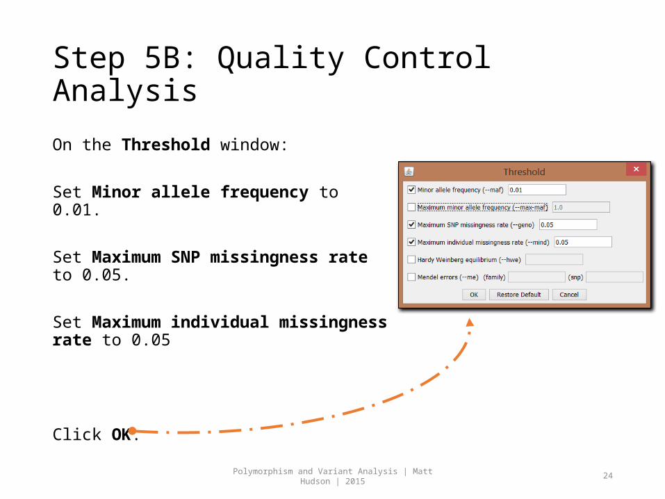
Step 5B: Quality Control Analysis

On the Threshold window:

Set Minor allele frequency to 0.01.

Set Maximum SNP missingness rate to 0.05.

Set Maximum individual missingness rate to 0.05

Click OK.


25

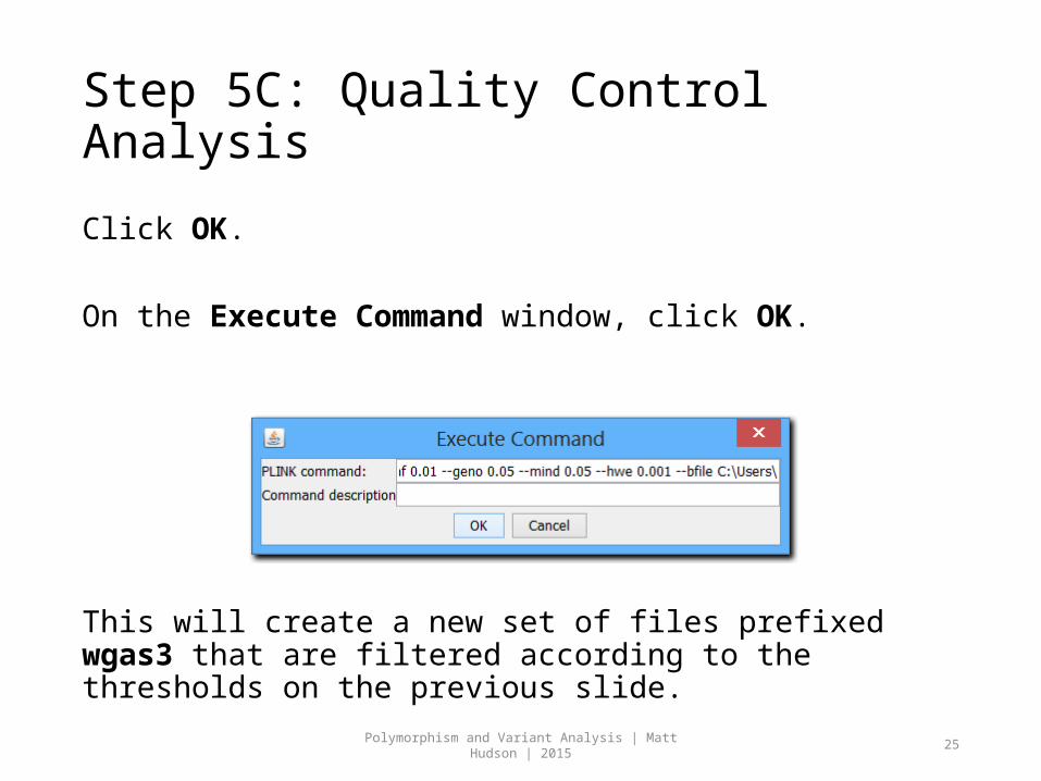
Step 5C: Quality Control Analysis

Click OK.


This will create a new set of files prefixed wgas3 that are filtered according to the thresholds on the previous slide.


26

Genome Wide Association Test (GWAS)In this exercise, we will a GWAS on our filtered data across two phenotypes: a case study and control. We will then compare the results between unadjusted p-values and multiple hypothesis corrected p-values.


27

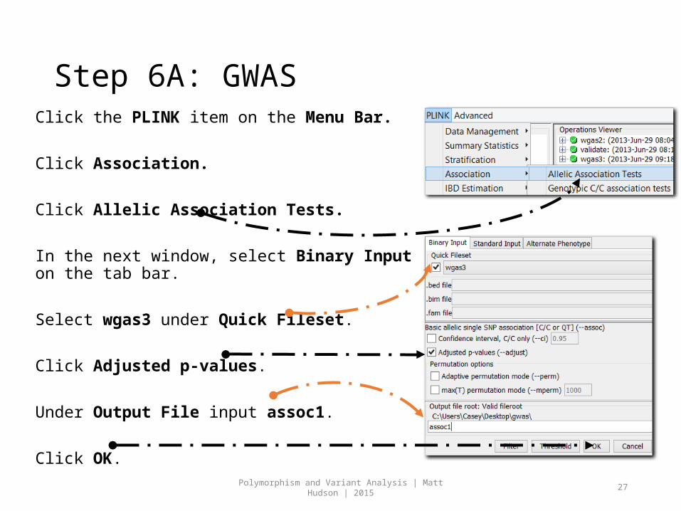
Step 6A: GWASClick the PLINK item on the Menu Bar.

Click Association.

Click Allelic Association Tests.



Click Adjusted p-values.

Under Output File input assoc1.

Click OK.


28

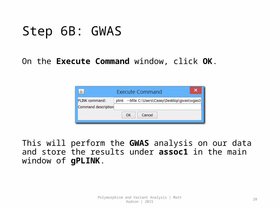
Step 6B: GWAS


This will perform the GWAS analysis on our data and store the results under assoc1 in the main window of gPLINK.


29

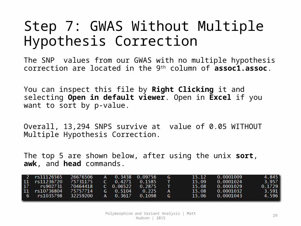
Step 7: GWAS Without Multiple Hypothesis CorrectionThe SNP values from our GWAS with no multiple hypothesis correction are located in the 9th column of assoc1.assoc.

You can inspect this file by Right Clicking it and selecting Open in default viewer. Open in Excel if you want to sort by p-value.

Overall, 13,294 SNPS survive at value of 0.05 WITHOUT Multiple Hypothesis Correction.

The top 5 are shown below, after using the unix sort, awk, and head commands.


30

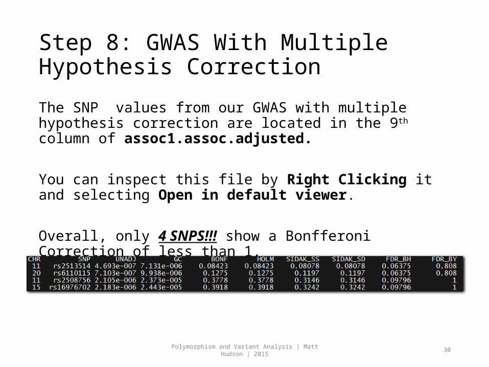
Step 8: GWAS With Multiple Hypothesis Correction

The SNP values from our GWAS with multiple hypothesis correction are located in the 9th column of assoc1.assoc.adjusted.

You can inspect this file by Right Clicking it and selecting Open in default viewer.

Overall, only 4 SNPS!!! show a Bonfferoni Correction of less than 1.


31

VisualizationIn this exercise, we will generate a Manhattan Plot of our association results using Haploview from the Broad Institute.


32

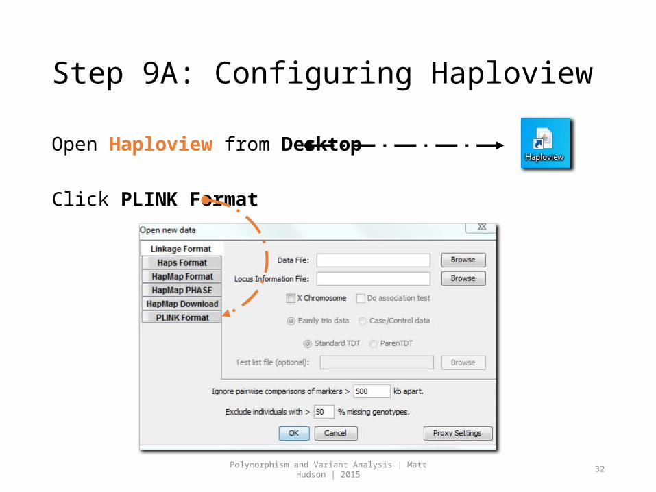
Step 9A: Configuring Haploview

Open Haploview from Desktop

Click PLINK Format


33

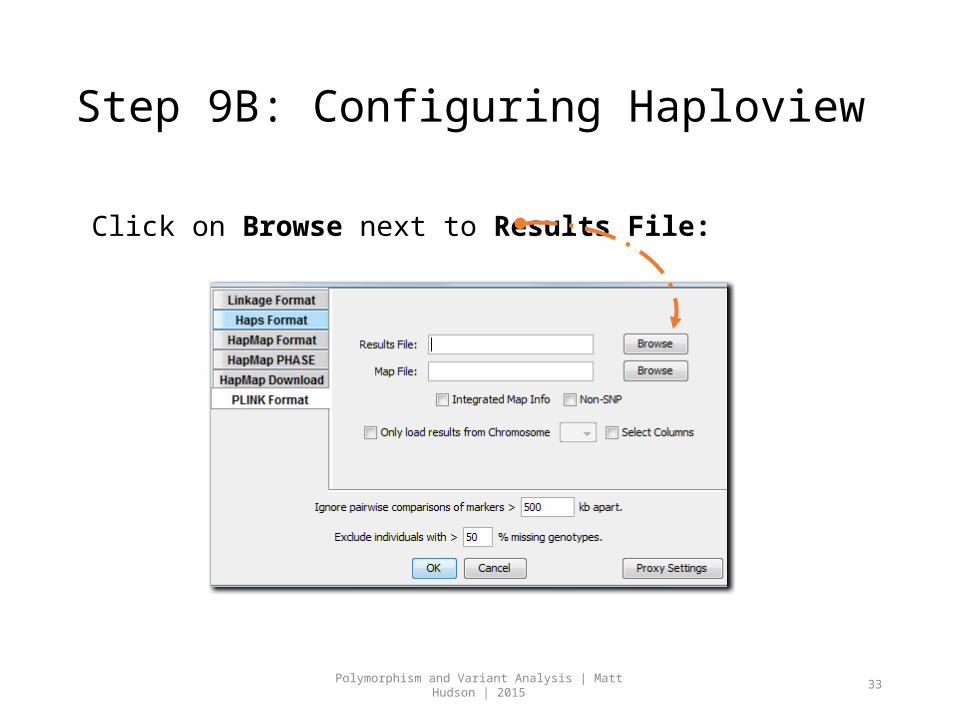
Step 9B: Configuring Haploview

Click on Browse next to Results File:


34

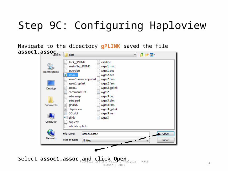
Step 9C: Configuring Haploview

Navigate to the directory gPLINK saved the file assoc1.assoc.

Select assoc1.assoc and click Open.


35

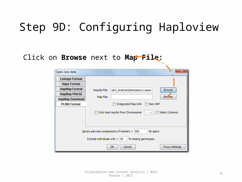
Step 9D: Configuring Haploview

Click on Browse next to Map File:


36

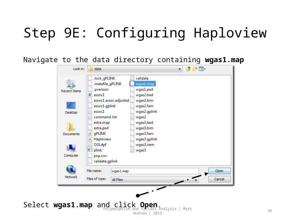
Step 9E: Configuring Haploview

Navigate to the data directory containing wgas1.map

Select wgas1.map and click Open.


37

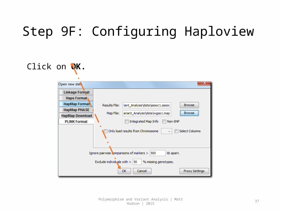
Step 9F: Configuring Haploview

Click on OK.


38

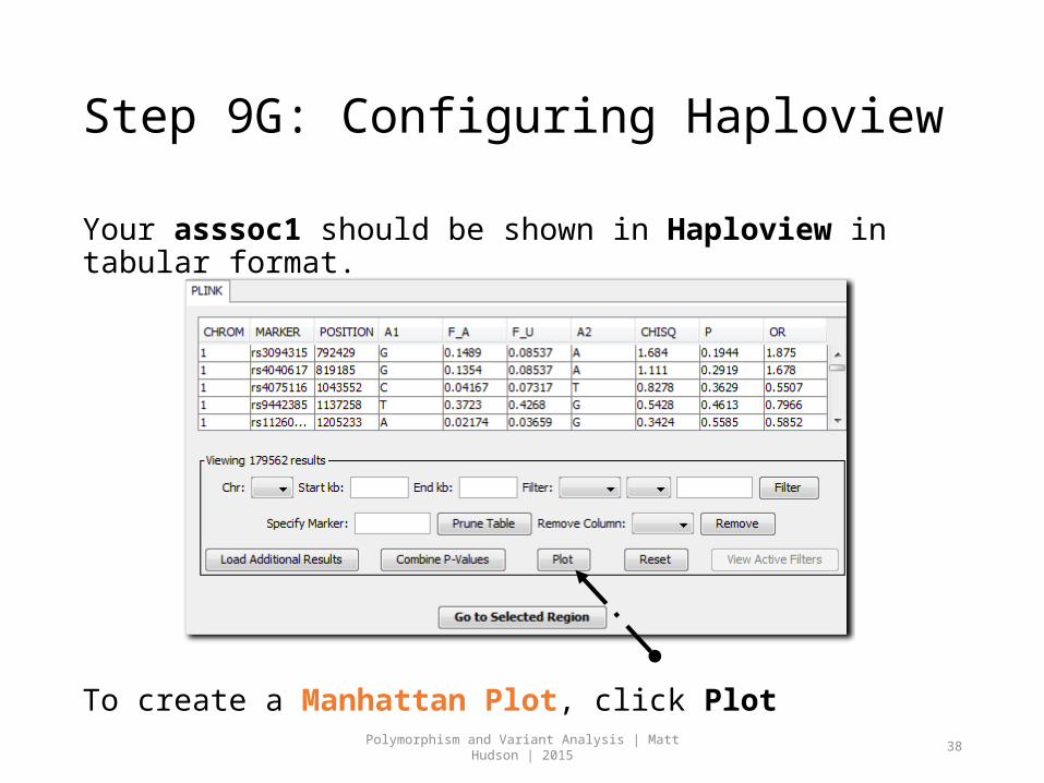
Step 9G: Configuring Haploview

Your asssoc1 should be shown in Haploview in tabular format.

To create a Manhattan Plot, click Plot


39

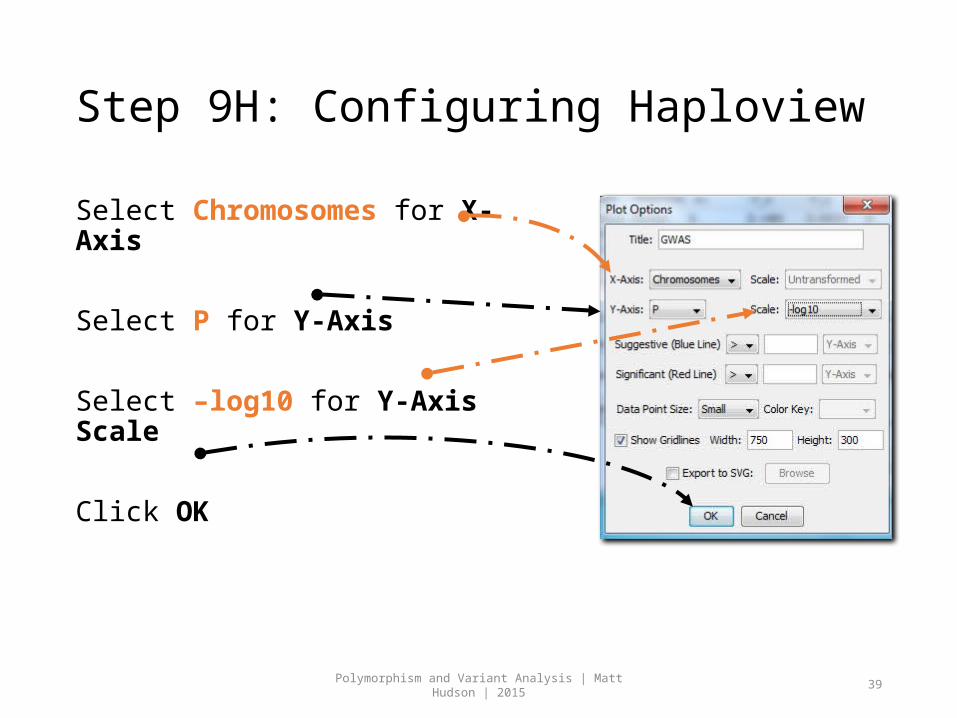
Step 9H: Configuring Haploview

Select Chromosomes for X-Axis

Select P for Y-Axis

Select –log10 for Y-Axis Scale

Click OK


40

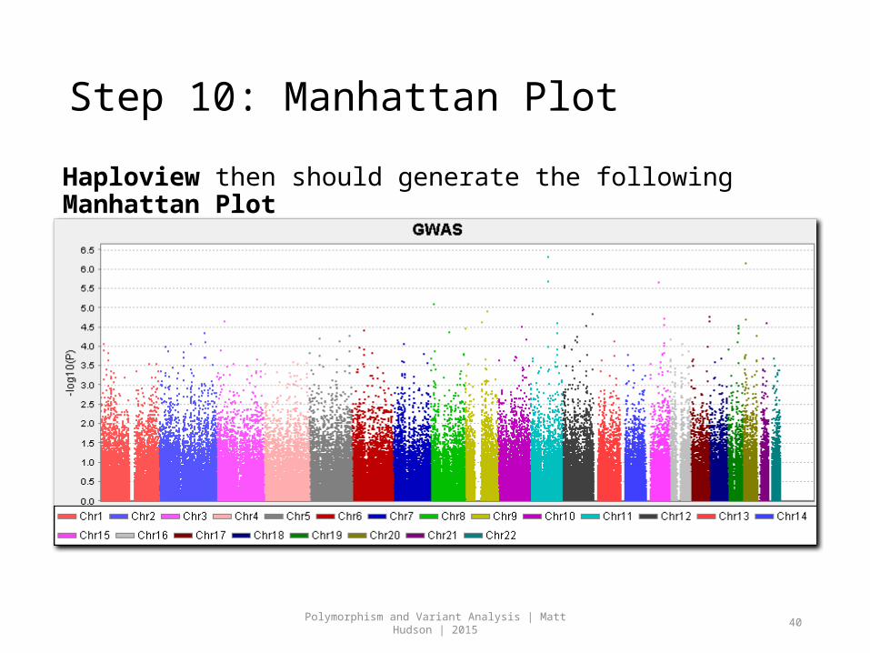
Step 10: Manhattan Plot

Haploview then should generate the following Manhattan Plot

Polymorphism and Variant Analysis Lab Matt Hudson Polymorphism and Variant Analysis | Matt Hudson |...

Documents

Transcript of Polymorphism and Variant Analysis Lab Matt Hudson Polymorphism and Variant Analysis | Matt Hudson |...