POLYMER STRUCTURES AND · PDF fileABSTRACT Investigations relating to dilute solutions of...
112
OFFICIAL PROJECT ASD TECHNICAL REPORT 61-22 RECORD Co.y. L C vp4t. POLYMER STRUCTURES AND PROPERTIES E. F. Casassa, T. A. Orofino, J. W. Mickey, T. G. Fox, G. C. Berry, D. J. Plazek, R. E. Kerwin, H. Nakayasu, V. R. Allen, C. A. J. Hoeve, M. O'Brien MELLON INSTITUTE 0 ooq a /6 AERONAUTICAL SYSTEMS DIVISION BEST AVAILABLE COPY
Transcript of POLYMER STRUCTURES AND · PDF fileABSTRACT Investigations relating to dilute solutions of...
OFFICIAL PROJECT
ASD TECHNICAL REPORT 61-22 RECORD Co.y.
L C vp4t.
POLYMER STRUCTURES AND PROPERTIES
E. F. Casassa, T. A. Orofino, J. W. Mickey,
T. G. Fox, G. C. Berry, D. J. Plazek, R. E. Kerwin,
H. Nakayasu, V. R. Allen, C. A. J. Hoeve, M. O'Brien
MELLON INSTITUTE
0 ooq a /6AERONAUTICAL SYSTEMS DIVISION
BEST AVAILABLE COPY

DHISC Lh
ThIS DOCUMNT iS BEST
iQUALIY AVAILABLE. Tht COPY
"FURNISHD TO DTIC CONTAINED
A SIGNIFICANT NUMBER OF
PA("ES W.ICH DO NOTý-JLJf GIB IX
REPRODUCED FROMBEST AVAILABLE COPY

ASD TECHNICAL REPORT 61-22
POLYMER STRUCTURES AND PROPERTIES
E. F. Casassa, T. A. Orofino, J. W. Mickey,T. G Fox, G. C. Berry, D. J. Plazek, R. E. Kerwin,
H. Nakayasu, V. R. Allen, C. A. J. Hoeve, M. O'Brien
Mellon Institute
Directorate of Materials and ProcessesContract No. AF 33(616)-6968
Project No. 0(7-7340)
AERONAUTICAL SYSTEMS DIVISIONUNITED STATES AIR FORCE
WRIGHT-PATTERSON AIR FORCE BASE, OHIO
?1OT fRELEASABLE TO OTS
FOREWO D
This report was prepared by Mellon Institute under USAF ContractNo. AF 33(616)-6968. This contract was initiated under Project No. 0(7-7340),"Polymer Structures and Properties," Task No. 73404. The work was adminis-
tered under the direction of the Directorate of Materials and Processes,Deputy for Technology, Aeronautical Systems Division.
This report covers work conducted from February 1, 1960 toApril 30, 1961.
ABSTRACT
Investigations relating to dilute solutions of polymers havecomprised: a theoretical treatment of Rayleigh scattering to include bothintramolecular and intermolecular optical interference effects; thetemperature dependence of the second virial coefficient for polystyrenein cyclohexane; the intrinsic viscosity-molecular weight relation forpoly-(vinyl acetate) in butanone; and design and construction of a precisionlight scattering photometer.
The melt viscosity-molecular weight relation at 2180 formonodisperse polystyrene prepared anionically was found to be identicalwith that for ordinary fractions.
Poly-(vinyl acetate), prepared by an emulsion polymerizationin the presence of a protein, yielded an insoluble component containingbound protein.
Preliminary stress-strain measurements on cross-linked swollenpolyethylene gave only equivocal evidence for specific solvent effects onthe unperturbed random-flight dimensions of the polymer chains.
PUBLICATION REVIEW
This report has been reviewed and is approved,
FOR THE CONMANDER:
A. M. LOVELACEChief, Poyler BranchNonmetallic laterials LaboratoryDirectorate of :<aterials & Processes
iii

TABLE OF CONTENTS
PART I DILUTE SOLUTION STUDIES
Page
I. Theory of Rayleigh Scattering from Solutions of Polymers:Effect of Intermolecular Correlations - Edward F. Casassa .... 1
A. Introduction ......................... *...........* ........ I
B. Theory for Linear Macromolecules ......................... 2
C.- The Single Contact Approximation ......................... 6
D. An Approximate Theory for Multiple Contacts .............. 8
E. Discussion ........ .... 14
II. Dimensions of Polymers--Specific Solvent Effects - T. A.Orofino, J. W. Mickey and T. G Fox ........................... 16
A. Introduction .......... . ... ..... ..................... 16
B. Experimental. Virial Coefficient-Temperature Studies onPolystyrene-Solvent Systems .................... 17
1. Selection of polymer molecular weight ................ 172. Phase studies and selection of solvents .............. 183. Osmotic pressure studies ................... 184. Light scattering studies ............... * ... 25
C. Theoretical. The Molecular Weight Dependence of theIntrinsic Viscosity in Polymer Solutions. A Comparisonof Theory and Experiment .......... ....... 99.......... 27
1. Introduction ... * #..... .............. . . . .. . . . ... 272. Theoretical [u]-M relationships ...................... 283. Derivation of K-from data on good solvents ... . ........ 294. The ([]-M relationship at high molecular weight ...... 335, The [r•j-M relationship at low molecular weight ....... 39
D. Summary and Conclusions ................................. 40
iv

TABLE OF CONTENTS - continued
Page
III. Light Scattering Photometer - G. C. Berry, E. F. Casassa,
and D. J. Plazek ................................................. 41
A. Introduction ................................................ 41
B. Apparatus ................................................. 41
1. General description .................................... 412. Optical design ......................................... 413. Optical alignment ....................................... 464. Electrical design ................................... ... 485. Electronic performance ................................. 506. Choice of the photomultiplier tube ...................... 527. Choice of the light source ............................. 538. Performance ............................................ 53
C. Conclusion .................................................. 55
D. Future Work ................................................. 55
IV. Viscosity - Molecular Weight Relationship for Poly-(Vinyl
Acetate) - R. E. Kerwin and H. Nakayasu ......................... 55
A. Introduction ............................................... 55
B. Experimental ............................................... 56
C. Results and Discussion ...................................... 58
D. Conclusion .................................................. 61
Appendix I ........................................................... 62
Appendix II .......................................................... 64
Appendix III ......................................................... 66
Bibliography ......................................................... 67
v
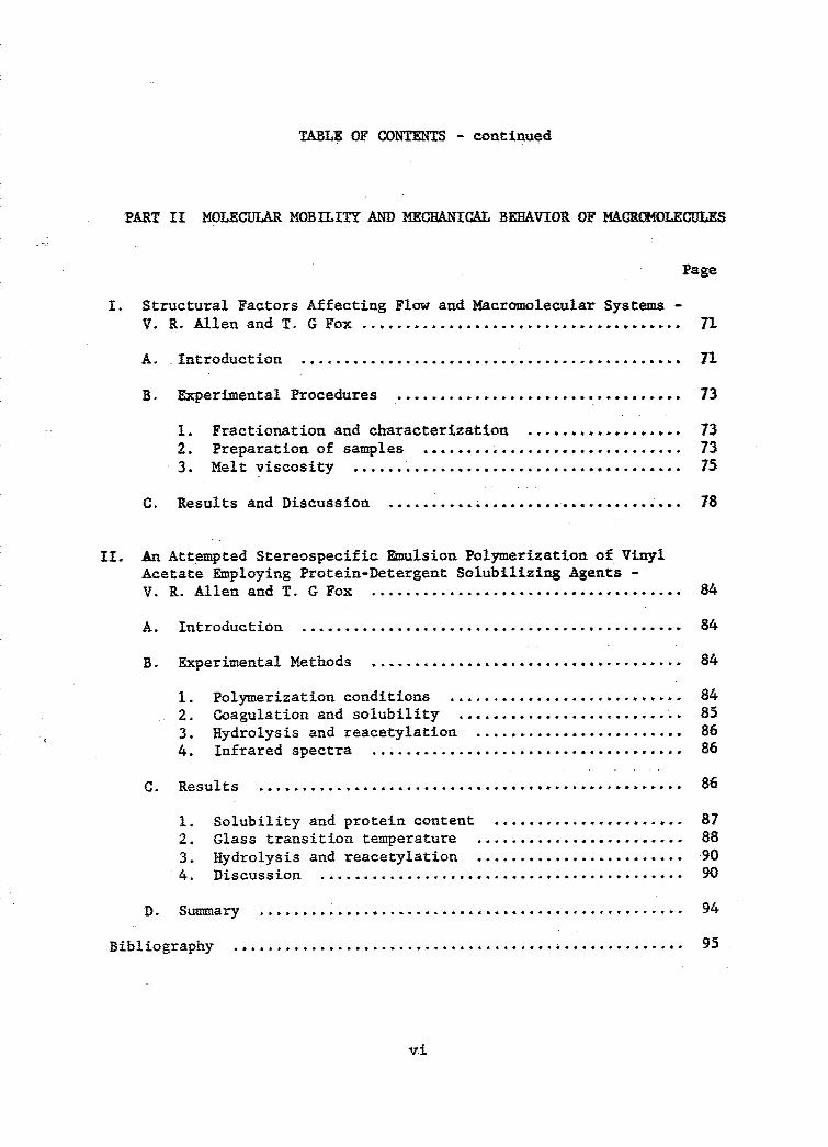
TABLE OF CONTENTS - continued
PART II MOLECULAR MOBILITY AND MECHANICAL BEHAVIOR OF MACRCZOLECULES
Page
I. Structural Factors Affecting Flow and Macromolecular Systems -
V. R. Allen and T. G Fox ...................................... 71
A. Introduction ............................................ 71
B. Experimental Procedures ................................. 73
I. Fractionation and characterization .................. 732. Preparation of samples ............................... 733. Melt viscosity ....................................... 75
C. Results and Discussion ................................... 78
II. An Attempted Stereospecific Emulsion Polymerization of VinylAcetate Employing Protein-Detergent Solubilizing Agents -V. R. Allen and T. G Fox .................................... 84
A. Introduction ............................................ 84
B. Experimental Methods ........................ ............ 84
1. Polymerization conditions ........................... 842. Coagulation and solubility .......................... 853. Hydrolysis and reacetylation ......................... 864. Infrared spectra .................................... 86
C. Results ................................................. 86
i. Solubility and protein content ...................... 872. Glass transition temperature ........................ 883. Hydrolysis and reacetylation ........................ 904. Discussion ......................................... 90
D. Summary ................................................. 94
Bibliography .................................................... 95
Vi

TABLE OF CONTENTS - continued
PART III ELASTICITY OF POLYMERIC NETWORKS
Page
I. Specific Diluent Effects on the Elastic Properties of
Polymeric Networks - C. A. J. Hoeve and M. OtBrien .......... 96
A. Introduction ............................................ 96
B. Procedure ................................................ 97
C. Experimental ............................................. 98
D. Results and Discussion .................................. 99
Bibliography . .................................................... 100
vii
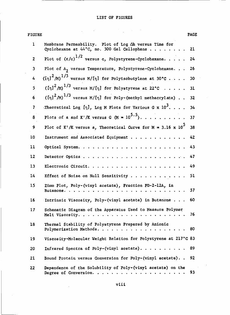
LIST OF FIGURES
FIGURE PAGE
I Membrane Permeability. Plot of Log 6h versus Time forCyclohexane at 440C0 no. 300 Gel Cellophane ........ 21
2 Plot of (if/c)1/2 versus c, Polystyrene-Cyclohexane...... 24
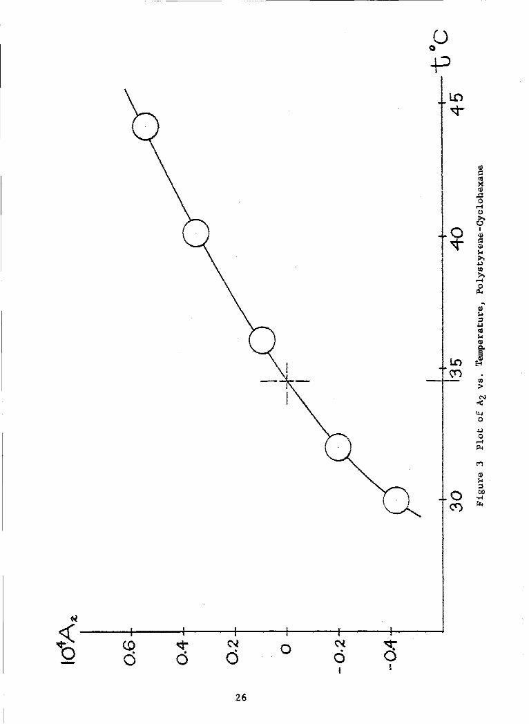
3 Plot of A2 versus Temperature, Polystyrene-Cyclohexane. . . 26
4 ([112/M)1/3 versus M/([] for Polyisobutylene at 30CC . . . 30
5 ([112/M)1/3 versus M/[n] for Polystyrene at 22.C ..... ... 31
6 ([P42/M)I/3 versus M/fi4 for Poly-(methyl methacrylate) 32
7 -Theoretical Log (n], Log M Plots for Various G x 10 . ... 34
8 Plots of a and KV/K versus G (M4- 10 5.5l ) ............. .. 37
9 Plot of KI/K versus a, Theoretical Curve for H = 3.16 x 10⁵ 38
10 Instrument and Associated Equipment ..... ............ ... 42
11 Optical System ............. ....................... ... 43
12 Detector Optics ........ .......................... 47
13 Electronic Circuit ........... ..................... ... 49
14 Effect of Noise on Null Sensitivity .................. 51
15 Zimm Plot, Poly-(vinyl acetate), Fraction PD-2-12A, inButanone ....................... ....................... 57
16 Intrinsic Viscosity, Poly-(vinyl acetate) in Butanone . . 60
17 Schematic Diagram of the Apparatus Used to Measure PolymerMelt Viscosity ........... ....................... ... 76
18 Thermal Stability of Polystyrene Prepared by AnionicPolymerization Methods ......... ................... ... 80
19 Viscosity-Molecular Weight Relation for Polystyrene at 217 0 C 83
20 Infrared Spectra of Poly-(vinyl acetate) .............. ... 89
21 Bound Protein versus Conversion for Poly-(vinyl acetate). . 92
22 Dependence of the Solubility of Poly-(vinyl acetate) on theDegree of Conversion.. ................................ 93
viii
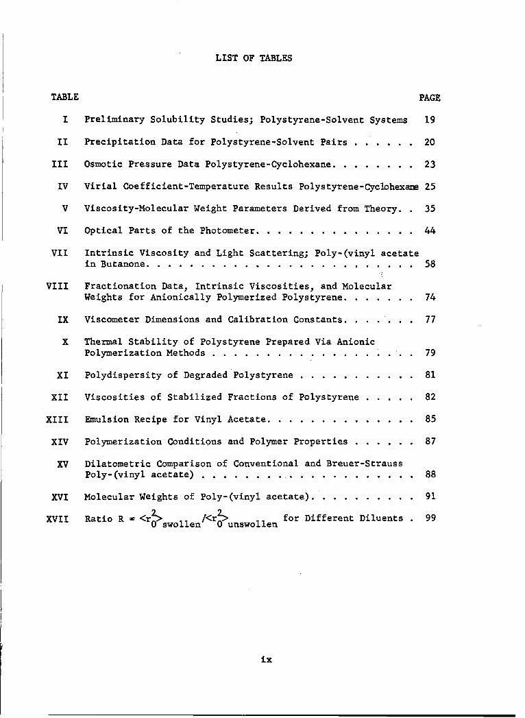
LIST OF TABLES
TABLE PAGE
I Preliminary Solubility Studies; Polystyrene-Solvent Systems 19
II Precipitation Data for Polystyrene-Solvent Pairs .......... 20
III Osmotic Pressure Data Polystyrene-Cyclohexane ........... ... 23
IV Virial Coefficient-Temperature Results Polystyrene-Cyclohexane 25
V Viscosity-Molecular Weight Parameters Derived from Theory.. 35
VI Optical Parts of the Photometer ...... .............. .... 44
VII Intrinsic Viscosity and Light Scattering; Poly-(vinyl acetatein Butanone ................ ......................... ... 58
VIII Fractionation Data, Intrinsic Viscosities, and MolecularWeights for Anionically Polymerized Polystyrene ........... 74
IX Viscometer Dimensions and Calibration Constants ........... 77
X Thermal Stability of Polystyrene Prepared Via AnionicPolymerization Methods ........... ............... . ... . 79
XI Polydispersity of Degraded Polystyrene .... ........... ... 81
XII Viscosities of Stabilized Fractions of Polystyrene ........ 82
XIII Emulsion Recipe for Vinyl Acetate ...... .............. ... 85
XIV Polymerization Conditions and Polymer Properties ........ .. 87
XV Dilatometric Comparison of Conventional and Breuer-StraussPoly-(vinyl acetate) ........... ..................... .. 88
XVI Molecular Weights of Poly-(vinyl acetate) .............. ... 91
XVII Ratio R = <r?>swollen/0 unswollen for Different Diluents . 99
ix

PART I - DILUTE SOLUTION STUDIES
I. Theory of Rayleigh Scattering from Solutions of Polymers: Effect ofIntermolecular Correlations - Edward F. Casassa
A. Introduction
The problem of the dependence of Rayleigh scattering fromdilute polymer solutions upon solute concentration and scattering anglehas been solved exactly only for special cases of limited applicabilityor more generally only for approximate molecular models. The difficultiesencountered do not pertain to the electromagnetic calculation per se:that is, the customary formulation1 ' 2 involving the classical electro-magnetic theory for scattering centers embedded in a medium of slightlydifferent dielectric constant appears to be altogether adequate now thata long-standing controversy concerning the local electric field actingon a scatterer has been resolved. 3 However, the intramolecular andintermolecular optical interference effects which determine the form ofthe angular scattering envelope depend on the configurational statisticsof the dissolved polymer molecule; and hence all the formidable difficultiesencountered in the statistical theory of real polymer chains with excludedvolume must appear also in the light scattering problem. In calculatingthe scattering from a system with the aid of statistical mechanics oneevidently develops in effect an equation of state in virial form or, moreprecisely, a series expression which reduces to the purely thermodynamicvirial expansion when the interference effects vanish.
The most complete treatment of scattering from polymer solutionswas initiated by Zimm4 who utilized the molecular distribution functionsof McMillan and Mayer 5 to obtain a theory valid to the approximation thatin accounting for intermolecular interactions only configurations withsingle contacts between pairs of solute molecules need be considered. Inmore recent work, Albrecht 6 has extended Zimm's method to include bimolecularclusters with two intermolecular contacts. Although some valuable gener-alizations can be inferred from the results carried to this approximation,further progress in the exact treatment is obstructed by difficulties whichappear nearly insuperable, even for machine computations; and thus muchinterest attaches to approximate molecular models for which calculation isfeasible. One such model was devised by Flory and Krigbaum, T'. whorepresented a polymer molecule by a Gaussian distribution of chain segmentsspherically symmetrical about the molecular center of mass, and thermodynamicinteraction between two molecules as the interpenetration of two such "soft"spheres. Flory and Bueches then used this model in studying the lightscattering problem.
Manuscript released by authors May 1961•for publication as an ASD TechnicalReport.
1
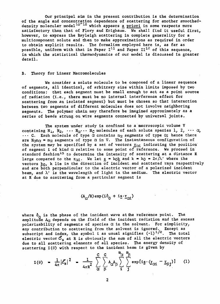
Our principal aim in the present contribution is the determinationof the angle and concentration dependence of scattering for another smoothed-density molecular model 1 0- 1 2 which appears a priori in some respects moresatisfactory than that of Flory and Krigbaum. We shall find it useful first,however, to express the Rayleigh scattering in complete generality for amulticomponent solute and then to make approximations as required in orderto obtain explicit results. The formalism employed here is, as far aspossible, uniform with that in Paper I11 and Paper 1112 of this sequence,in which the statistical thermodynamics of our model is discussed in greaterdetail.
B. Theory for Linear Macromolecules
We consider a solute molecule to be composed of a linear sequenceof segments, all identical, of arbitrary size within limits imposed by twoconditions: that each segment must be small enough to act as a point sourceof radiation (i.e., there must be no internal interference effect forscattering from an isolated segment) but must be chosen so that interactionbetween two segments of different molecules does not involve neighboringsegments. The polymer chain may therefore be imagined approximately as aseries of beads strung on wire segments connected by universal joints.
The system under study is confined to a macroscopic volume Vcontaining NI, N2 , ... Na... NC molecules of each solute species 1, 21 ...... C. Each molecule of type a contains na segments of type a; hence thereare Nana - ma segments of type a in V. The instantaneous configuration ofthe system may be specified by a set of vectors ai indicating the positionof segment i of kind a relative to some point of reference. We proceed instandard fashion1 3 to determine the intensity of scattering at a distance Rlarge compared to the rai. We let s = kot and k = ko = 21f/X' where thevectors ½0, k lie in the direction of incident and scattered rays respectivelyand are both perpendicular to the electric vector of a polarized incidentbeam, and V is the wavelength of light in the medium. The electric vectorat R due to scattering from a particular segment is
(a R)exp(i60 + is-%ad
where 65 is the phase of the incident wave atthe reference point. Theamplituae A, depends on the field of the incident radiation and the excess
polarizability of segments of species a in the solvent. For simplicity,any contribution to scattering from the solvent is ignored. Except as
subscript and index, the symbol i as usual signifies (-l)1/2. The total
electric vector5s at R is obviously the sum of all the electric vectorsdue to all scattering elements of all species. The energy density ofscattering 1(e) with respect to the incident beam is given by
1ni2 1 -(r'~ r r.1(e) = A A •-AA -exp[i i - LJ 1 (1)i4iR 2 H U
2
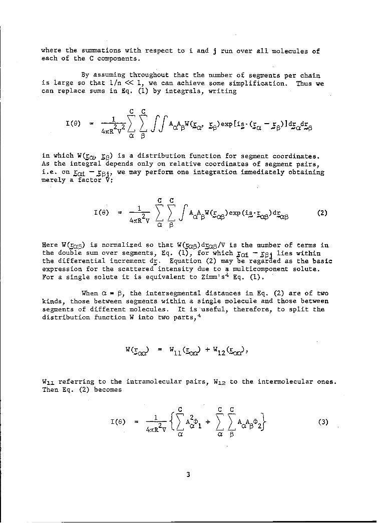
where the summations with respect to i and j run over all molecules ofeach of the C components.
By assuming throughout that the number of segments per chainis large so that 1/n << 1, we can achieve some simplification. Thus wecan replace sums in Eq. (1) by integrals, writing
C C(e) = / ( r )exp[is. - r )ldr dr
a -
in which W(ra, Sp) is a distribution function for segment coordinates.As the integral depends only on relative coordinates of segment pairs,i.e. on rci -- r, we may perform one integration immediately obtainingmerely a factor V:
C C
1(e)1 7 fA A W(r )exp(is.-a )dra (2)a
Here W(rya) is normalized so that W(rcb•)drcE/V is the number of terms inthe double sum over segments, Eq. (1), for which rod - rj lies withinthe differential increment dr. Equation (2) may be regarAed as the basicexpression for the scattered intensity due to a multicomponent solute.For a single solute it is equivalent to Zimm's 4 Eq. (1).
When a = P, the intersegmental distances in Eq. (2) are of twokinds, those between segments within a single molecule and those betweensegments of different molecules. It is useful, therefore, to split thedistribution function W into two parts, 4
W(r = Wll() + W1 2 (r ,
W11 referring to the intramolecular pairs, W1 2 to the intermolecular ones.Then Eq. (2) becomes
C C C
1(G) A 2{7'2 + 7 7A CA 2 1 (3)4TcR 2 V f
a a
3
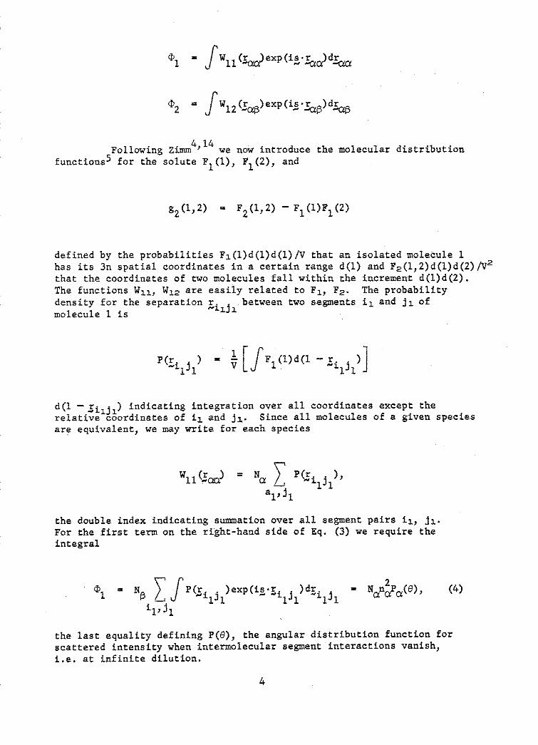
S"fWI(r~exp(is-rd•
1 = 1iQa)Iaýd a
f27WI 2 rc)exp(is - )d1
Following Zimm 4 we now introduce the molecular distributionfunctions 5 for the solute FI(1), F1 (2), and
g2 (1, 2 ) = F21(,2) - F1(1)F1(2)
defined by the probabilities F1 (l)d(l)d(1)/V that an isolated molecule 1has its 3n spatial coordinates in a certain range d(l) and F2 (1,2)d(l)d(2)NV2
that the coordinates of two molecules fall within the increment d(l)d(2).The functions W1 1 , W12 are easily related to F1 , F2 . The probabilitydensity for the separation r. . between two segments i 1 and ji ofmolecule 1 is •L31
)~ ='E F (l) d(1 111 'il -V
d(l- ri.1 l) indicating integration over all coordinates except therelative coordinates of il and jl. Since all molecules of a given speciesare equivalent, we may write for each species
Wlltc) N= a P1 ,j
the double index indicating summation over all segment pairs il, j,.For the first term on the right-hand side of Eq. (3) we require theintegral
21 N 73 P(rilJl )exp(is-ri li)drilil
1- )*i*J 1.,~j Nanj(e), (4)
the last equality defining F(e), the angular distribution function forscattered intensity when intermolecular segment interactions vanish,i.e. at infinite dilution.
4

The function F2 (1,2) has now to be introduced into the integralD2 of Eq. (3). From the definitions above it is evident that
P(r = - 'F(l112)d(l)d(2 - rl)(qlq 2 V 2 2
qlq2
and
Wl2(r) = NaN 7 F(r qlq2)
ql q2
qj, q 2 designating segments of molecules 1 and 2 of types a and •. Toproceed, we factor F2 (1,2) in the way prescribed by Zimm4
F 2 (l,2) = F1(1)F 1 (2) q Ci - X(il, i2]
il i 2
and expand the product. Since the short-range interaction functions Xare zero except when the segments in question are in contact, they mayproperly be represented by three-dimensional Dirac delta functions. 1 5
Combining these expressions we have:
( 2 N= • T FF (1)FI(2)FI - X(il 1 i 2 )
V ql q q2 i13_ i2
+ 7' X(ii )X(J , ) +"
(il, i 2 , jlj 2 )
x d(l)d(2 - r )exp(is. )dl (5)
The first term of 02
exp(is- dr
5

relates to the surface scattering from the volume V. It will be omittedin all that follows since it is negligible at experimentally accessiblescattering angles.
Again invoking the short range nature of the X functions wecan set r -r. - r and factor the second term of Eq. (5) toobtain ýqlq2 -i2 q2 filq,
N aN 13 X~ l' pp ex ~ s-
ily i2' ql, q2
p~ NNXJP(ri )exp(is-r )dr. C-ý- n2n 2X P (ep (e) (6)
I ri 2 q2 "ep is 2 q)2 -V 2q2 V c2cza a
The integral of X(il,i2), denoted by Xap (B in Papers I and II), is takento be the same for all segment pairs of each type a- f-
C. The Single Contact Approximation
So far, the treatment has been rigorous with respect to theproperties of the string-of-beads molecular model and represents simplya generalization of Zimmt s theory to more than one solute component. Infact, since the probability densities remain unspecified no characteristicof the model except the short range nature of interactions has yet beenused. Albrecht's 6 work comprises the evaluation of the third term inEq. (5) for a single solute component. It is only in this term thatprobabilities of intermolecular contacts dependent on chain statisticsfirst appear. By combining Eqs. (4) and (6) in Eq. (3), we obtain thescattering from the system:
C C C2 V2 2 I41rR vi(e) - A&1aN, (e) - A? IA ANcnaNpn X P (e) P (e) + (7)
at a l
Expressing concentrations c in the customary units of mass/volume, andwriting the amplitudes Aa, Ap in terms of the refractive increments
ta= -)/6ca etc., with l the refractive index of the solution, we obtainan expression of the more familiar fDrm
K 1-K 1 + 2A (e)
R(&) 2 2
a
6
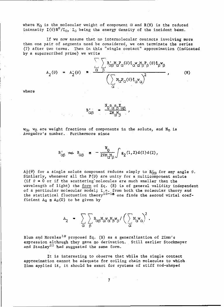
where Ma is the molecular weight of component a and R(e) is the reducedintensity I(e)R2 /Io, Io being the energy density of the incident beam.
If we now assume that no intermolecular contacts involving morethan one pair of segments need be considered, we can terminate the series(7) after two terms. Then in this "single contact" approximation (indicated
by a superscribed prime) we write
L_ Bý 5NMP(8)ý waMNPP (e)w W
A2 (e) = A'(6) a , " 2 (8)
awhere
N n nX
wa, wt are weight fractions of components in the solute, and No isAvogadro's number. Furthermore since
N0B -• B• -= 2v# g(1, 2) d(1) d(2),
Ak(e) for a single solute component reduces simply to BI for any angle e.Similarly, whenever all the P(e) are unity for a multicomponent solute(if G = 0 or if the scattering'•molecules are much smaller than thewavelength of light) the form of Eq. (8) is of general validity independentof a particular molecular model; i.e. from both the molecular theory andthe statistical fluctuation theoryis-is one finds the second virial coef-ficient A2 5 A2 (0) to be given by
A2 P Z aMawaM~~ (7Paa)aý a
Blum and Morales' 9 proposed Eq. (8) as a generalization of Zimm'sexpression although they gave' no derivation. Still earlier Stockmayerand Stanley2 0 had suggested the same form.
It is interesting to observe that while the single contactapproximation cannot be adequate for coiling chain molecules to which
Zimm applied it, it should be exact for systems of stiff rod-shaped
7

particles.1 4 Hence for a distribution of rod species or a mixture ofrods and small molecules (with P(e) unity) Eq. (8) gives A2 (e) withoutapproximation. In certain rather simple cases, therefore, it should bepossible to determine the interaction coefficients Ba3 from the dependenceof A2 (9) on e, in measurements on a single composition of a mixed solute.This has been accomplished in at least the one instance2 1 of solutionsof mixtures of the plasma protein fibrinogen and a rod-like polymericform.
D. An Approximate Theory for Multiple Contacts
In devising-a theory in which all orders of intermolecularcontacts are included we are obliged to resort to some approximationwhich renders tractable the higher members of the series of integralsin Eq. (5). We therefore adopt the simplificationl elaborated inPapers I and II that probabilities of intermolecular contacts may beexpressed as products of probabilities for single contacts. Explicitly,we assume that
P(OJlJ21'Ok1k2 01 2 1)22 1 )2Ol 12i2P(Ok1k2)1i2... P(O 1m2)1 12
P(OJZJ2)ili2l for example, denoting the conditional probability of acontact between segments J1, J2 given the "initial" intermolecular contactbetween segments i1 and i 2 . With the consistent additional assumptionthat the separation rqlq2 depends only on the initial contact, Eq. (5)is replaced by
0 "O Z 1 - (~7~ 0 jJii1'i 2' qlq q2 Jl1 J2
+ 2 2Jl' J2.,klk k2
XJP(i. )XPs(isr. )d.q f P(r )exp(isrq )d_lql t oilql lq2 f -Vi2 q 2 2 2q2 w2 q 2
8

As we pointed out earlier the series in square brackets can be summedto give
1-expEX 7O ",P(O. )~
2 v Xcx pil'i 2 X P(O 2)ili
X fP(r. )exp(is-r. )dr. f P~r )exp(is-r. )dr. (9)ý ý i1q 1 -ilql_ - 1q ri 2 q2 -i 2 q2 -t2q2
ql, q2
At this point it is necessary to introduce a specific form for theprobabilities in Eq. (9). We take them to be given by random-flightstatistics although it is not strictly correct to do so when chainsexhibit an intramolecular excluded volume effect. (If this is the case,Xaa does not vanish and the distribution function F, does not correspondto a random flight. 1 2 ) Assuming therefore that
P(r ) = [(2icb2/3)Iq- i1 ]-3/2exp(-3r2. 11q - ill2b2) (10)
we obtain
I P(r. )exp(isr. 2:r. PQr. )r cos(sr cos e)sin e dedrilql 1 1 q 3.i1qI10 0-0 0
=exp(-1q 1 - ijs2b2 /6)
where b 2 is the mean square segment length or mean square separationbetween beads of the chain (assumed now to obey a Gaussian distribution).We substitute this result into Eq. (10), introduce the random-flightvalues1 I of the contact probabilities P(0J1 3 2 )i i2 , etc., and replacesums by integrals. The integrations over q, and q2 are readily performedleaving finally an intractable double integration over il and i2 .
Since it would be a cumbrous affair Lo obtain numerical resultsfor a multicomponent system from the approximate (2 derived by thisprocedure, we shall consider further only the simplest, but difficult
9

enough, case of a homogeneous solute, for which a = •. Thus, suppressingthe greek subscripts and using the reduced variables x il/n, y 1 ia/n,we obtain from Eq. (9)
D -2 N2n4Xfj (, w) f (u, x) f (u, y) dxdy (11)
00
in which
(?Pw) =
I= 2x1/2 + 2y1/2 + 2(l x)1/2 + 2(l y)i/2 (x + y)1/ 2
--(i - + Y)i1/2 _ I+ x y)i1/2 _(2 -- x- y)i1/2, (12)
-. (12)u(1'X
f(ux) = u-(2 - eux - eU(lx)i,
f(uy) a u- (2 e - euU(l-Y)
= 4xnl/2(312nb2 ) 33/2
u M 6ns s <r /(7 sin
<r 2 > a * nb2 being the mean square molecular radius for the random flightchain. We shall use the star to designate quantities consistent with theassumptions leading to Eq. (11).
Recalling that A2 (e) approaches the second virial coefficientA2 a A2 (0) as e approaches 0, we may define a new angular scatteringfunction
P2 (e) = A2 (B)/A2 (0)
g (I2) Z (i- rq)d(l)d(2 )
njfg(l02)d(l)d(2)
10

for a cluster of two molecules, analogous to P(e) for a single molecule.Then the general expression for scattering from a homogeneous solute maybe written
R(e) = Kc[MP(e) - ZA2 M 2P 2 (e)c + .]
or
Kc 1
R(e) 7P(-0) + 2A2 Q(e)c + "'" (13)
where
Q(e) = P2 (e)/P 2(e)
The function Q(6) is thus unity, by definition, at zero angle, andordinarily decreases with increasing angle. Apart from its directoccurrence in the reciprocal scattering expression, Q(G) is convenientfor tabulation since, as a measure of deviations from the single contactapproximation, it may be expected to vary less rapidly with e than doesP2 0(). As we have already assumed random-flight statistics in developingthe approximate expression, Eq. (11), it is consistent to use the random-flight model again in introducing P(O), i.e. to let
= 2 -uP(G) - [u +e -1] (14)
2U
in
Q Me _e2 (P2(ef 1~ - exp (-ý) dxdy) (15)
00
An exact analytic evaluation-of Q (e) appears impossible; buteven wfthout resorting to numerical integration, we can investigate thebehavior of the function in certain limiting cases and'in approximation.If thermodynamic interactions are weak (that is, if ý, and thus ' and
11
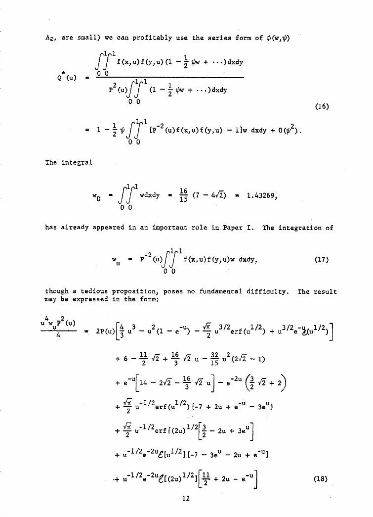
A2 , are small) we can profitably use the series form of k(w,4')
101 1f(xfu)f (y -u)(l j w+ ... )dxdy
* 00Q (u) - 1
P 2(u (1 - -w + ... )dxdy
0 0 (16)
-- 1 - " f [P 2 (u) f (x, u) f (y, u) - liw dxdy + 0(42).
00
The integral
W fO wdxdy - 16 - 41) - 1.43269,
00
has already appeared in an important role in Paper I. The integration of
w P- 2(u)j f(x,u)f(y,u)w dxdy, (17)
00
though a tedious proposition, poses no fundamental difficulty. The resultmay be expressed in the form:
w'uP (uu)3 _2 u u3/2 (ul/2) u3/2e-(ul/214 - L2P(u)JL u3 u2( -- e 2 erf +
iI 6 1ý2 6 r2u_32 u2 (2-/ -1
2 3 15
+ eu[14 - 2Y-u -1 l6 ;2 u] - 2u 317+ 2)
VT-12 / -u
+ U-1/2 erf(u 1/2)[-7 + 2u +e -- 3 eu]
* -- u 1/2 erf[(2u) 1 /2 - 2u + 3 eu
+ u-1 / 2 e 2u 8[ul/2j [-7 - 3 eu - 2u + e-u]
-1/2 -2ue 1/2] ii 1U+ e- l[(2u) ][T + 2u - euj
12
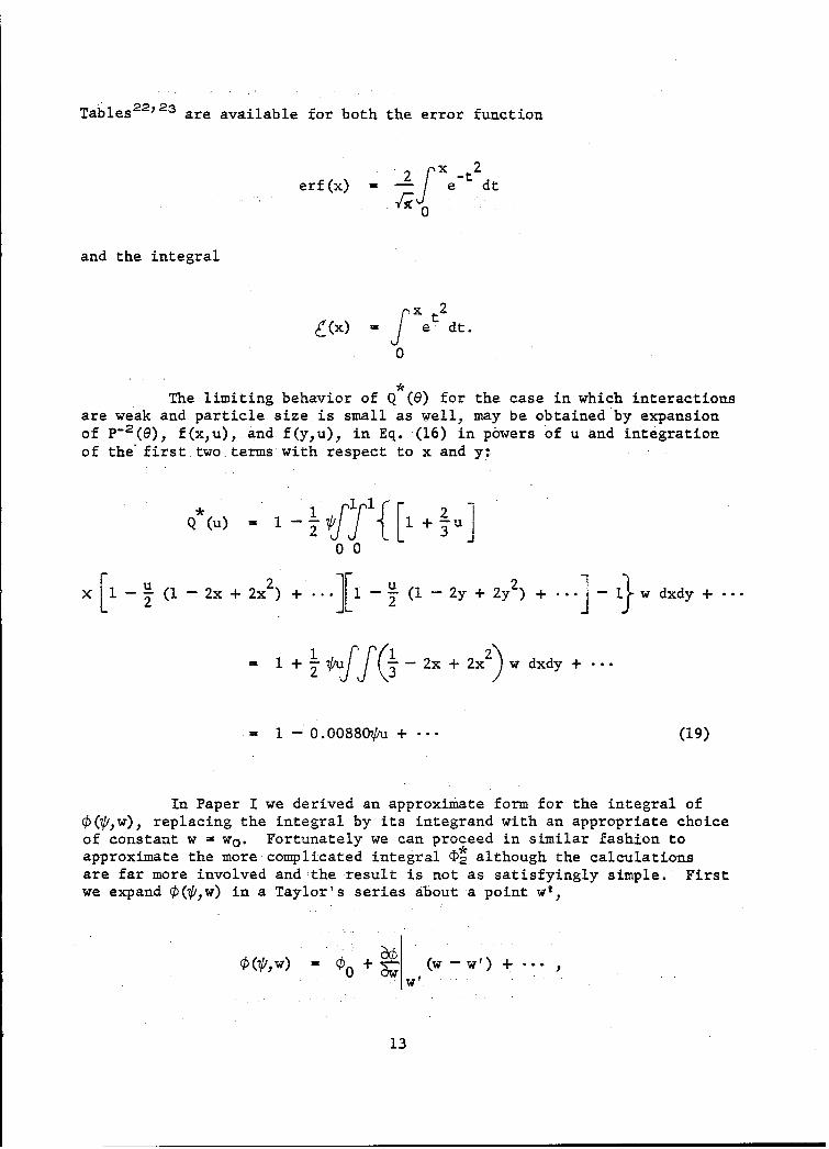
Tables 2 2 ', 2 are available for both the error function
erf(x) 2 e dt
0
and the integral
•(x) fxet 2dt.
0
The limiting behavior of Q (e) for the case in which interactions
are weak and particle size is small as well, may be obtained by expansionof p-2(e), f(x~u), and f(y.,u), in Eq. (16) in powers of u and integration-of the'first two terms with respect to x and y;
Q (u) 2 + 3- l -uO00
X I-•(I -- 2x + 2x 2 + .. i- (1 -- 2y + 2y2) + .. . w dxdy +--
= 1 + 1 -- 2x + 2x.2 w dxdy +--
= I - .oo880op + .. (19)
In Paper I we derived an approximate form for the integral of0(?Pw), replacing the integral by its integrand with an appropriate choiceof constant w f wo. Fortunately we can proceed in similar fashion to
approximate the more complicated integral (D2 although the calculationsare far more involved andwthe result is not as satisfyingly simple. First
we expand 0(?Pw) in a Taylor's series about a point wt,
00
,w l+ +u f( (w-2 2w d +. ...,
= -0.O8 Wu (9
InPaerI edeivd naproimtefrmfo teinegalo

and then, after multiplying by f(x)f(y), integrate the series term byterm with respect to x and y to obtain
I>*
S2(w')p 2 (u) + ; // (w - w t)f(x)f(y)dxdy +
00
As in the earlier work we neglect the higher terms and causethe second to vanish by a proper choice of w'. That is, we let
ff wf(x)f(y)dxdy - w'P2 (u)
00
hence w' is identical with w of Eq. (18). Then 02* is given by
-ID /N2n 4XP2 (e) -:, 00 (w)-[- exp (-u It/*;2
and finally using this, together with the same approximation for theparticular case u - 1,
f (7, w) dxdy j [ exp (-- 0 0,
in Eq. (15) gives for an approximation to Q (e)
** wo 1 - exp (-4v, )Q (e) = uu [ exp - 0) ] (20)
E. Discussion
The function Wu, which depends only on the value of u, is equalto wo at u = 0 and increases slowly as u increases. Therefore as either"4' or u increases positively (with neither zero), Q*(e), at least initially,decreases gradually from unity; that is, it decreases as thermodynamicinteractions become stronger or as the scattering molecules become larger.
14

That this behavior is correct qualitatively, is shown bycomparison with the (almost) exact treatment of Albrecht.6 Quantitatively,though, our theory predicts only a very small effect; for Q (6) canscarcely be more than a few per cent less than unity for physicallyrealizable values of u and 7P. Albrecht's theoretical development givesthe first two terms of a power series
Q(e) - 1 - 0.074u'1 + ... (21)
which is to be compared with our Eq. (19) above. The wide discrepancyin the coefficients of the linear terms does not of course prove anythingabout the behavior of the closed form, Eq. (20), at large values of wu,but it does suggest that this series may well be seriously inadequate.
The only other theory available for comparison is that of Floryand Bueche 9 based on the Flory-Krigbaum molecular model. Their seriesexpansion of Q(e) gives
Q(e) 1 - 0.038u•f + (22)
and from numerical calculations for large values of u and ?P they find thatQ(e) may fall to about 0.5 for values of these parameters that are quitereasonable physically. It seems surprising at first sight that for smallvalues of u* the new theory shows much poorer agreement with Eq. (21) thandoes the Flory-Bueche expression, since in two respects the model we haveused appears superior. Inasmuch as it preserves the correct random-flightvalue for the separation of segment pairs within a molecule, it automaticallyyields the correct random-flight P(G). The averaging of the segment densitydistribution inherent in the Flory-Krigbaum model leads to a considerablydifferent function. 2 412 5 In view of this, Flory and Bueche retained theP(6) of Eq. (14) in their theory of Q(G) and used their model only inaccounting for the intermolecular interference effects. The second andmore significant consideration is that our model gives correctly thesimultaneous probability of two intermolecular distances (e.g. one segment-segment contact and one segment-segment separation) whereas the Flory-Buechetreatment is approximate in the specification of more than one such distance.Consequently, although the coefficient of the second term in the series forQ(e) depends on probabilities for simultaneous occurrence of three distances,it does not seem obvious why Eq. (19) should be more inaccurate than Eq. (22).
15
II. Dimensions of Polymers--Specific Solvent-Effects -- T. A. Orofino,J. W. Mickey and T. G Fox
A. Introduction
A number of years ago, Florysand co-workers advanced the theorythat the intrinsic viscosity of a polymer solution [Tq] may be expressed bythe relationship
M= K1/2 a3 (23)
where M is the polymer molecular weight and a is a factor by which thelinear dimensions of the polymer coil are expanded due to long-rangepolymer-solvent interactions. The constant K is a molecular weightindependent quantity defined
K ( 0 /M)3/2 (24)
2.where ro is the root mean square end-to-end distance (proportional to M)of the polymer chain in a solvent for which C is unity, and 0 is a universalconstant.
For any given polymer-solvent pair there exists a thermodynamicallysignificant temperature, e, at which a is unity. This temperature may bedetermined experimentally, as, for example, from an observation of thetemperature so at which the second virial coefficient A2 in the expressionfor the reduced osmotic pressure ,r/c
c = (//c)" [ + MA 2c + ... (25)
where c is polymer concentration, vanishes. (At temperatures a few degreesbelow e. the polymer solution separates into two phases.) Values of e havebeen recorded for many systems. 3 2 In accordan e with Eq. (23) the constantK may be evaluated from the ratio of [(T] and M14 in a e-solvent mixture,and, again, a number of values 3 1 for various polymers have been so determined.
16

On the basis of early measurementsZ8 33it was believed that Kwould to a first approximation be independent of the solvent chosen forany given polymer, although in general dependent upon temperature. Theeffects of the two variables, i.e. solvent and G-temperature, are noteasily separated and for this reason the constancy of K with solvent typehas not been unequivocally established to date for the systems studied.Moreover, there is experimental evidenceZ3,3 4 to support the notion that,indeed, variations of K with solvent type occur.
We may therefore conclude that the dimension of an isolatedpolymer coil, as reflected by such measurable quantities as the intrinsicviscosity and light scattering radius of gyration, in a e-solvent solutionwhere the net segment-solvent interaction is nil, may in general be presumedto depend upon two factors: (a) the temperature at which the particularpolymer-solvent pair is a e-mixture and (b) the chemical and physicalnature of the solvent molecule. The latter, in relation to the structuralcharacteristics of the polymer repeating unit, may impose certain conforma-tional restrictions upon relatively short sections of the polymer chain.We are interested in studying this effect, whose elucidation necessarilyinvolves control or elimination of factor (a) as a variable. On thisaccount, we have endeavored to select a number of solvent pairs for aparticular polymer, the members of each pair of which exhibit approximatelythe same e-temperature with the polymer chosen, but which differ considerablyin chemical type or structure. Thusfor any selected solvent pair, differ-ences in the e-solvent dimensions of the dissolved polymer, which it is ourobject to determine, may be meaningfully attributed to the specific shortrange polymer-solvent interaction, the more general, and obscuring, effectof temperature having been circumvented by selection of e-temperatures inapproximate juxtaposition.
In our current program we have selected polystyrene-solventsystems for study; the method of the dependence of the second virialcoefficient on temperature has been chosen for the definition of e-tempera-tures. In the next section, experimental results obtained to date arepresented and discussed.
In Section C a draft of a manuscript entitled "The MolecularWeight Dependence of the Intrinsic Viscosity in Polymer Solutions. AComparison of Theory and Experiment" is presented. Although somewhatmore general in scope, the results of this investigation are pertinentto the present project.
B. Experimental. Virial Coefficient-Temperature Studies on Polystyrene-Solvent Systems
1. Selection of polymer molecular weight. In selecting asingle polystyrene sample of suitable molecular weight for our investiga-tions, the following considerations were taken into account: The polymersample should be stable and relatively homogeneous, to minimize possiblecomplications of molecular weight polydispersity on the physical properties
17

of interest, and should be available in sufficient quantity for allmeasurements. The molecular weight should be high enough to (a) permitaccurate determinations of solution viscosities and (b) present no diffi-culties in diffusion through osmotic membranes. It should be sufficientlylow so that (a) shear corrections to the intrinsic viscosities areinconsequential (b) the polymer solutions do not exhibit phase separationuntil five or more degrees below the e-temperature and (c) dissymmetrycorrections in light scattering measurements are small.
With the above criteria in mind, we decided upon an optimummolecular weight of 3.5-4.5 X 10⁵. A thirty gram sample of anionicallypolymerized polystyrene meeting this specification was generously suppliedto us by co-workers in our laboratories.
2. Phase studies and selection of solvents. In the selectionof suitable solvents for our investigations, the objective was to obtaintwo or more solvent pairs, members of each pair of which exhibited approxi-mately the same e-temperature with polystyrene, and which preferablydiffered considerably in structure. As there is no way to predict thesolubility characteristics with any assurance of accuracy, a large numberof solvents was investigated by the following method: A small amount ofa readily available polystyrene sample was.added to the solvent underconsideration and the solubility, or lack of it, observed over a widerange of temperature. Our preliminary observations are recorded inTable I, where in the last column the approximate precipitation temperaturesnoted (which presumably are somewhat below the e-points for the systems)are listed.
On the basis of the data summarized in Table II four solventswere selected for more detailed investigation. For each of these,reversible precipitation temperatures of dilute solutions of a highmolecular weight polystyrene sample were determined in a water bathcontrolled to ±0.01°C. The precipitation temperatures observed may bepresumed to correspond, within a few degrees, to the respective e-pointsof the systems. Estimated values of the latter are listed in Table IItogether with other pertinent information. Listed also in Table II arevalues of 6 - 6psy the Hildebrand solubility parameter differences betweenthe solvents and polystyrene (6ps = 9.2). These differences may be regardedas semi-quantitative measures of the degree to which members of a given0-solvent pair are dissimilar in structure and polarity; it is desirablefor our purposes that values for a given pair exhibit opposite algebraicsigns, as is the case for the two pairs cited.
The estimated e-temperatures, boiling points and refractiveindices of the four solvents listed in Table II are such that it isfeasible to employ them as suitable media for polystyrene in osmoticpressure, light scattering and viscometric measurements. Our work inthe past and in the immediate future has been and will be confined tothese solvents.
3. Osmotic pressure studies. As mentioned earlier, it is our
aim to establish accurate values of the e-temperatures for a number of
18
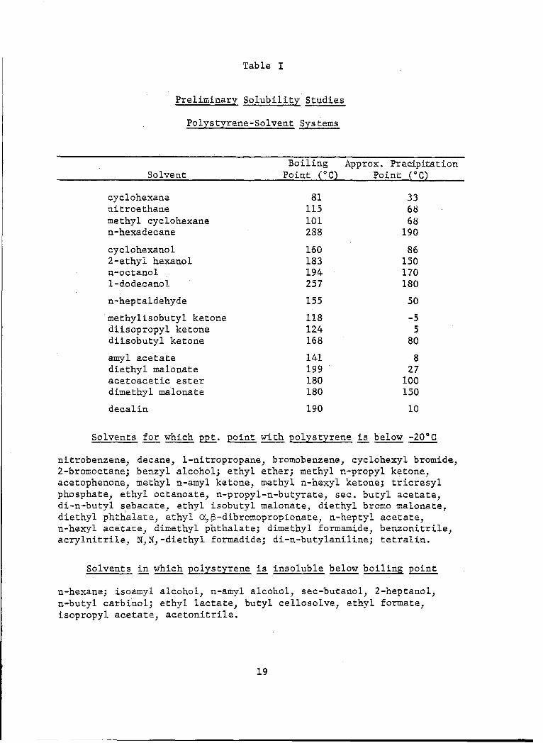
Table I
Preliminary Solubility Studies
Polystyrene-Solvent Systems
Boiling Approx. PrecipitationSolvent Point (°C) Point (°C)
cyclohexane 81 33nitroethane 115 68methyl cyclohexane 101 68n-hexadecane 288 190
cyclohexanol 160 862-ethyl hexanol 183 150n-octanol 194 1701-dodecanol 257 180
n-heptaldehyde 155 50
methylisobutyl ketone 118 -5diisopropyl ketone 124 5diisobutyl ketone 168 80
amyl acetate 141 8diethyl malonate 199 27acetoacetic ester 180 100dimethyl malonate 180 150
decalin 190 10
Solvents for which p£p. point with polystyrene is below -20'C
nitrobenzene, decane, l-nitropropane, bromobenzeneY cyclohexyl bromide,2-bromoctane; benzyl alcohol; ethyl ether; methyl n-propyl ketone,acetophenone, methyl n-amyl ketone, methyl n-hexyl ketone. tricresylphosphate, ethyl octanoate, n-propyl-n-butyrate, sec. butyl acetate,di-n-butyl s ebacate, ethyl isobutyl malonate, diethyl bromo malonate,diethyl phthalate, ethyl aa,-dibromopropionate, n-heptyl acetate,n-hexyl acetate, dimethyl phthalate; dimethyl formamide, benzonitrile,acrylnitrile, NN,-diethyl formadide; di-n-butylaniline; tetralin.
Solvents in which polystyrene is insoluble below boiling point
n-hexane; isoamyl alcohol, n-amyl alcohol, sec-butanol, 2-heptanol,n-butyl carbinol; ethyl lactate, butyl cellosolve, ethyl formate,isopropyl acetate, acetonitrile.
19

Table II
Precipitation Data for Polystyrene-Solvent Pairs
D Approx.
Solvent B.P. P2 5 (g/cc) n 2 5 5 - p e-temp.,°C
cyclohexane 81 0.779 1.4262 -1.0 34diethylmalonate 199 1.055 1.4143 +0.3 32
methyl cyclohexane 101 0.769 1.4231 -1.4 71nitroethane 115 1.047 1.3901 +1.94 71
polystyrene-solvent systems by interpolation of the temperature at whichthe second virial coefficient A2 for the system is zero. The lightscattering method is the most convenient procedure for evaluation of A2and will be extensively utilized in most of our work. It is desirable,however, to establish for one (or more) systems the value of e by anindependent means. We have completed a study of the osmotic second virialcoefficient-temperature relationship for polystyrene in cyclohexane, theresults of which are herein reported.
The osmometer used in our work was an all brass Fuoss-Mead blockinstrument with a membrane-capillary tube cross-section ratio of 4360.The membranes were wet regenerated cellulose, 300 gauge, obtained fromAmerican Viscose Corporation. Temperature control for the osmometer wasmaintained by means of a water bath, regulated by a sensitive thyratronrelay, enclosed in an insulated cabinet fitted with an air thermostat,heating element and blower. With this apparatus, temperatures in therange 30-45°C, measured with Beckman thermometers, could be maintainedwithin ±0.002 for extended periods and within less than ±0.001 for a fewhours. Reading of the capillary tube levels was accomplished by means ofa cathetometer scaled directly to 0.001 cm.
A typical membrane permeability plot for one of the membranesused in our study is shown in Fig. 1. The half-time computed from theslope is 56 minutes.
The procedure employed in the osmotic pressure measurementswas as follows: A solution of polystyrene in redistilled cyclohexanewas carefully prepared and allowed to stand overnight at a temperature(440C) well above the precipitation point. Taking care to avoid cooling,the solution was used to rinsel and eventually to fill, the osmometeralready at constant temperature (440 C) in the water bath. Preheated,long hypodermic needles and syringes were found useful in these opera-tions. After elimination of any bubbles, the osmotic pressure of thesolution at the filling temperature (the highest temperature employed
20

0
o _0
004
a
r4M
0 .
4)
to
Q
01
0
0
.9- 0 ,.
.0r
0l
d o40 0
210

in the series of measurements) was determined by allowing the levels toequilibrate from two directions - an initial setting of the difference insolution and solvent levels Ah greater than the equilibrium value Ah E anda setting of Ah less than AhE. The stable values obtained in the twodeterminations usually differd by less than 1-2%; the mean value was takenas the equilibrium difference in height.
Upon completion of measurements at the highest temperature, 440c,bath temperature was reduced to 40* and the osmotic pressure redetermined.Subsequently, measurement at 36, 32 and 30'C was carried out, at the endof which portions of the solution and solvent were withdrawn from theosmometer and analyzed by a dry weight determination of polymer. The osmometerwas then rinsed and filled with the next solution and fresh solvent.
The series of equilibriumAh values obtained for a given solutionwas converted to osmotic pressure units (g/cm2 ) by multiplication of each bythe density appropriate to the temperature of measurement and the polymerconcentration. For this purpose, the following relationships, establishedexperimentally, were used
p(t,c) = p(t,o) + (3.22)l0"•c
(2-6)
p(t,o) = 0.764 + (1.06)10-3(34-t)
where p(t,c) is the density of a polystyrene-cyclohexane solution of con-centration c g/lOO cc. at temperature t 0 c.
The osmotic pressure values it were divided by the appropriatesolution concentrations to yield the ratio it/c, which values are listed inTable III. The concentrations appropriate to each measurement were arrivedat as follows: from the dry weight concentration established at the end ofa temperature series, together with data for the progressive decrease of thesum of the heights of the capillary levels throughout the run, it was possibleto correct each concentration for the loss of solvent which had occurred fromthe beginning of a temperature series to the end of a measurement at a giventemperature. These corrections were usually of the order of 1% or less.The concentration values, corrected for evaporation, were then expressed inunits appropriate to the particular temperature of measurement.
The final osmotic data were plotted in accordance with the squareroot relationship
S(i/c)1/e = [RT/MnIi'1[1 + (A2Mn/2)cI (27)
22
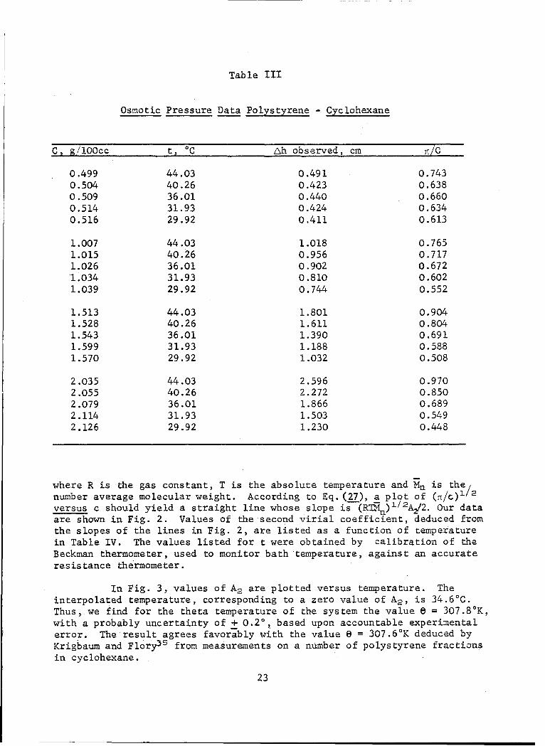
Table III
Osmotic Pressure Data Polystyrene - Cyclohexane
C, g/1OOcc t' C Lh observed, cm 'tiC
0.499 44.03 0.491 0.7430.504 40.26 0.423 0.6380.509 36.01 0.440 0.6600.514 31.93 0.424 0.6340.516 29.92 0.411 0.613
1.007 44.03 1.018 0.7651.015 40.26 0.956 0.7171.026 36.01 0.902 0.6721.034 31.93 0.810 0.6021.039 29.92 0.744 0.552
1.513 44.03 1.801 0.9041.528 40.26 1.611 0.8041.543 36.01 1.390 0.6911.599 31.93 1.188 0.5881.570 29.92 1.032 0.508
2.035 44.03 2.596 0.9702.055 40.26 2.272 0.8502.079 36.01 1.866 0.6892.114 31.93 1.503 0.5492.126 29.92 1.230 0.448
where R is the gas constant, T is the absolute temperature and Mn is the/number average molecular weight. According to Eq. (27), a plot of (I/C)lversus c should yield a straight line whose slope is-(RTRn)1/2A2/2. our dataare shown in Fig. 2. Values of the second virial coefficient, deduced fromthe slopes of the lines in Fig. 2, are listed as a function of temperaturein Table IV. The values listed for t were obtained by calibration of theBeckman thermometer, used to monitor bath temperature, against an accurateresistance thermometer.
In Fig. 3, values of A2 are plotted versus temperature. Theinterpolated temperature, corresponding to a zero value of A2 , is 34.6°C.Thus, we find for the theta temperature of the system the value e = 307.8°K,with a probably uncertainty of + 0.2°, based upon accountable experimentalerror. The result agrees favorably with the value 8 = 307.6°K deduced byKrigbaum and Flor9 5 from measurements on a number of polystyrene fractionsin cyclohexane.
23

41
0
C14
244

Table IV
Virial Coefficient-Temperature Results Polystyrene-Cyclohexane
(M = 4.04 x 10⁵)
t°c 1O4A2
44.03 0.543
40.26 0.350
36.01 0.093
31.93 -0.195
29.92 -0.420
4. Light scattering studies. We have recently begun lightscattering measurements, by means of which we plan to determine accurate8 temperatures for each of the four solvents listed in Table II. As inthe preceeding osmotic pressure studies, it is our intention to computethe S-temperatures by interpolation of the virial coefficient-temperaturerelationships. The light scattering virial equation analogous to Eq. (25)for osmotic pressure is
c/!t = (c/- )[l + 2A2Mc + ... 1 (28)
where T' is the excess turbidity, extrapolated to zero angle. Thus,determination of the scattering intensity as a function of angle, concen-tration and temperature for a given polystyrene-solvent system permitsevaluation of A2 as a function of temperature, from which G may be deduced.
The light scattering instrument at our disposal is a Brice-Phoenix unit which we are presently calibrating and adapting to ourparticular needs.
We have designed and constructed a thermostat by means of whichclose temperature control of the light scattering cell may be maintained.In the operating position, the cell rests on a hollow base through whichwater from a large constant temperature reservoir is recirculated viaheavily insulated conduits. A heavily insulated, double-wall jacket slipsover the cell and makes contact with the hollow base. Bath water is alsodirected through this jacket in an efficient manner by the placement of
25
0
'40
0-a
-4
0n
00
C) 1
26~
suitable baffles. We are presently in the process of determining therelationship between bath and cell temperatures, as a function of theformer, when the aforementioned assembly is in operation.
Calibration of the instrument has been completed and lightscattering measurements will be carried out in the near future.
C. Theoretical. The Molecular Weight Dependence of the IntrinsicViscosity in Polymer Solutions. A Comparison of Theory and Experiment*
1. Introduction. From a large amount of experimental datacollected over the years, one may ascertain certain general characteristicsof the molecular weight dependence of the intrinsic viscosity of linearpolymers. It is the purpose of this communication to investigate theextent to which theoretical relationships currently available are able toaccount for and, to some degree, elaborate upon the more important of thesefeatures observed.
Over a limited, although often quite useful, range of polymermolecular weights M, the intrinsic viscosities [(Ti of a given polymer--solvent system at a specified temperature may be adequately representedby a semi-empirical relationship of the Mark-Howink form
[TIJ = K'Ma (29)
where K' and a are constants characteristic of the particular system
investigated. Values of these parameters have been determined for a largenumber of polymer-solvent pairs in the range of molecular weights normallyof interest for characterization purposes, about 105 - 106.
The parameter a in most cases assumes values between 0.5 and 0.8and, in magnitude, is qualitatively associated with the solvent power ofthe medium. The constant K' is usually in the range 10-3 - 10"- and for agiven polymer in a series of solvents (or in a given solvent at varioustemperatures) tends to decrease with increasing a.
For some polymer-solvent pairs, investigated over wide ranges ofmolecular weights, two relationships of the form (29),with different valuesof the constants, have been used to describe the systems; one set ofparameters is applicable to the region of low molecular weight, (less thanabout 3 x 10⁴), the other, with a larger value of a, to the region ofmoderate to high molecular weight. Systems 3 8 have been studied in whicha for the low molecular weight region was found to be 0.5, a value usuallyassociated with e-solvent systems over the entire molecular weight range(cf. seq.).
This section represents in part a manuscript which is to be submittedfor publication.
27
2. Theoretical [q]-M relationships. According to the Flory-Foxrelationship3 9 , the intrinsic viscosity of a linear polymer is given by theexp ress ion
[rI] = D(r2 /HM)3/2N-/&3 = M•-/2a3 (30)0
where r 2 proportional to M, is the unperturbed root mean square end-to-endQ
separation of chain ends in a S-solvent mixtttre, D is a constant (about2.2 x 1021 for most systems, with [rjj in deciliters/g.) and a is an expansionfactor by which the linear dimensions of the molecular coil are assumed tobe increased by segment-solvent interactions. The latter quantity may beoperationally defined
a= ((•J/(•] 8 )-/3 (31)
where [I]e is the intrinsic viscosity of the specified polymer of givenmolecular weight, at a specified temperature, in a 9-solvent mixture.According to the theory4 0 , of intra molecular interactions, the parametera may be expressed by the relationship
Oa- P = 2Cm04(l - e/T)MN/2 = GMý/a (32)
where C is a constant previously defined4 1 , 4i and S are interactionmparameters characteristic of the polymer-solvent pair and T is the absolutetemperature. Higher terms are neglected4 2 . When the right hand side ofthe above equation becomes zero, as it does, for example, at the uniquetemperature T = 8 for a given polymer-solvent pair, a becomes unity, [rj],in accordance with Eq. (31), reduces to [T]jJ and the intrinsic viscosity-molecular weight relationship of Eq. (30) becomes
[ile = R,1/2 ; K = (9--/-) 3/2 (3)
The constant K is independent of polymer molecular weight. It may beexpected to vary somewhat with temperature through its dependence on theunperturbed root mean square end-to-end distance, and, taking into accountpossible effects on the latter arising from short range specific solventinteractions, may in general depend to some degree upon the nature of themedium in which the polymer is dissolved. Evidence for the latter efforthas been noted in the case of cellulose derivatives. 4 3
Values 3 9 ' 4' of K for a number of different polymers have beenderived from e-solvent intrinsic viscosity measurements in accordance withthe first of the equations (33).
28
An alternate, indirect method for the determination of K valuesfrom viscosity data in good solvents was suggested a number of years ago39A variant of this procedure has been developed recently by Kawai and Naito37.
In the next section, the details of the original treatment are examined andare applied to data on a number of polymer-solvent systems.
3. Derivation of K from data on good solvents. Equations (8)and (10) of the preceding section may be combined, with elimination of a,to yield the relationship39
([•]2/M) /3 = K2/3 + K5/3G(M/[ 1I]) (34)
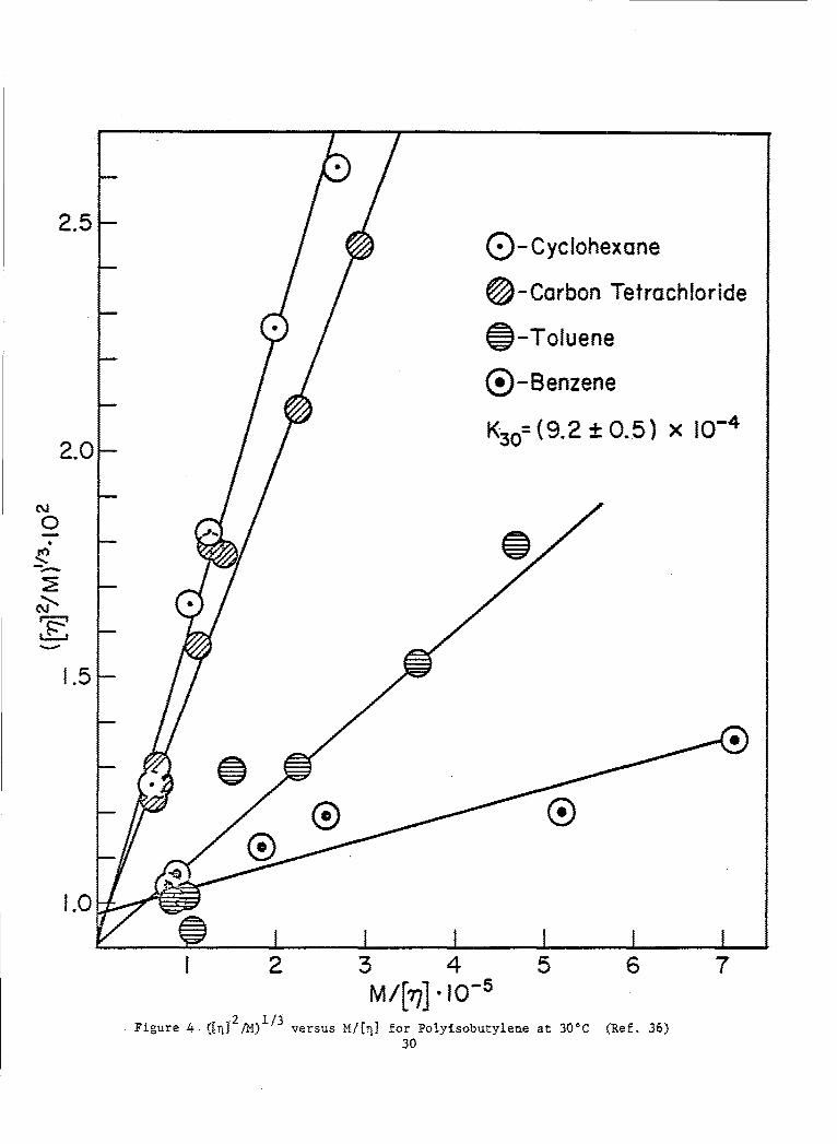
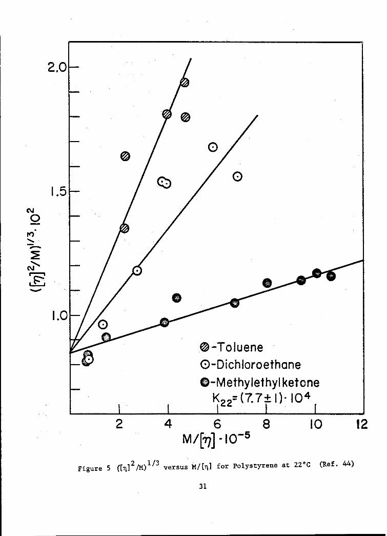
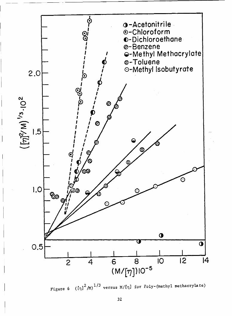
Thus, according to theory, a plot of ([11]2/M)1/3 versus M/[,q] for anypolymer-solvent system/at a given temperature should produce a straightline with intercept K2'/3 and slope K5 / 3 G. Graphs for the systems poly-isobutylene 6, polystyrene-4 and polymethylmethacrylate in varioussolvents are shown in Figs. 4, 5, and 6 respectively. The dataappear to describe linear relationships in all cases, although in somethere is considerable scatter. In the polyisobutylene and polystryenesystems, common intercepts, within experimental error, are obtained. Therespective values of K derived from these intercepts are 9.2 and 7.7 x jo-4
in reasonably good agreement in each case with those values (at the sametemperature) deduced from e-solvent viscometric data3 9 ' 10.6 and 8.0 x 10⁻⁴.With the exception of the curves for chloroform and dichloroethane, thedata on polymethylmethacrylate also yield a common intercept, correspondingto a K value of 4.4 x 10⁻⁴, which stands in good agreement with the value4 6
4.8 x 10⁻⁴ deduced from e-solvent measurements. Possible explanations forthe apparent anomolies observed in the case of the two aforementionedsolvents are 1. the existence of specific solvent effects which couldconceivably alter the K values appropriate to these systems, 2. failureto take into account higher terms in Eq. (32) the effect of which may besignificant in these cases* , and 3. other deficiencies in theory.
Everything considered, the procedure described for the determina-tion of K values from good solvent data does appear to afford a usefulmeans of polymer characterization when direct evaluation of K from 9-solvent measurements is impracticable or inconvenient. Moreover, themethod described, when applied with objective reservation, may serve as auseful guide in the detection and evaluation of specific solvent effects.
*The equivalent version of Eq. (34) with retention of the second order
interaction term7 in Eq. (32) is of the form
([T2]/M)i/3 = K2/3 + K5/3G(M/[rj]) + KS/3H(Ml/2/[rf]2)
where H is a molecular weight independent quantity proportional to thesecondary interaction parameter (1/3 - X2 ). The additional term couldconceivably make a significant contribution at low values of M/[L], inline with the deviations observed in the two solvents cited.
29
2.5- (Q-Cyclohexone
0D-Carbon Tetrachloride
(D-Toluene
®-Benzene
2.0- K-30=(9.2±0.5) X 10- 4
0
('J
1.5
1.0
12 3 4 5 6 7MI['i7] 'J -5
Figure.4. ([rIJ 2 'm) 13versus M'/tj] for Polyisobutylene at 30'0 (Ref. 36)30
2.0-
0
1.5-
00
1.0-1.0
,0-Toiuene
O-Dichloroethane0-Methylethyl ketone
K22= (7.7- 1)- 1 i 4
2 4 6 8 10 12M/['/] - 10-5
Figure 5 ([rI]2/M)I/ 3 versus M/[b] for Polystyrene at 22 0 C (Ref. 44)
31
@o-Acetonitrile®D-Chlorof ormc-Dichloroethane
I @-Benzene@-Methyl Methocrylate
I c-Toluene2.0) -Methyl Isobutyrate
20-
ID
1.0-
2 4 ý6 8 10 12 14
2M [ý 1/35
Figure 6 ([n] 44M)1 versus 14/[I for Poly-(methyl methacrylate)
32
4. The [n]- relationship at high molecular weight.
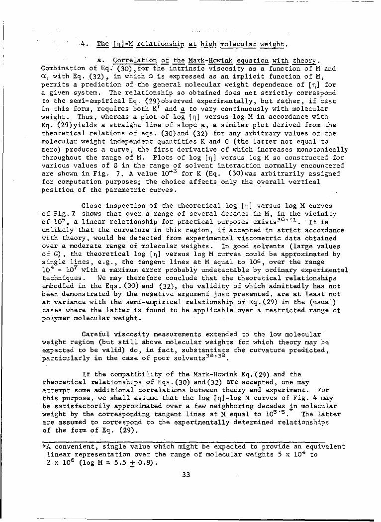
a. Correlation of the Mark-Howink equation with theory.Combination of Eq. (30),for the intrinsic viscosity as a function of M anda, with Eq. (32), in which U is expressed as an implicit function of M,permits a prediction of the general molecular weight dependence of [n] fora given system. The relationship so obtained does not strictly correspondto the semi-empirical Eq. (29)observed experimentally, but rather, if castin this form, requires both K' and a to vary continuously with molecularweight. Thus, whereas a plot of log [ri] versus log M in accordance withEq. (29)yields a straight line of slope a, a similar plot derived from thetheoretical relations of eqs. (30)and (32) for any arbitrary values of themolecular weight independent quantities K and G (the latter not equal tozero) produces a curve, the first derivative of which increases monotonicallythroughout the range of M. Plots of log [n] versus log M so constructed forvarious values of G in the range of solvent interaction normally encounteredare shown in Fig. 7. A value 10-3 for K (Eq. (30)was arbitrarily assignedfor computation purposes; the choice affects only the overall verticalposition of the parametric curves.
Close inspection of the theoretical log [il versus log M curvesof Fig. 7 shows that over a range of several decades in M, in the vicinityof 105, a linear relationship for practical purposes exists 3 6
*41. It isunlikely that the curvature in this region, if accepted in strict accordancewith theory, would be detected from experimental viscometric data obtainedover a moderate range of molecular weights. In good solvents (large valuesof G), the theoretical log [l] versus log M curves could be approximated bysingle lines, e.g., the tangent lines at M equal to 105, over the range10 - 107 with a maximum error probably undetectable by ordinary experimentaltechniques. We may therefore conclude that the theoretical relationshipsembodied in the Eqs. (30) and (32), the validity of which admittedly has notbeen demonstrated by the negative argument just presented, are at least notat variance with the semi-empirical relationship of Eq.(29) in the (usual)cases where the latter is found to be applicable over a restricted range ofpolymer molecular weight.
Careful viscosity measurements extended to the low molecularweight region (but still above molecular weights for which theory may beexpected to be valid) do, in fact, substantiate the curvature predicted,particularly in the case of poor solvents36236
If the compatibility of the Mark-Howink Eq.(29) and thetheoretical relationships of Eqs.(30) and(32) are accepted, one mayattempt some additional correlations between theory and experiment. Forthis purpose, we shall assume that the log [rl]-log M curves of Fig. 4 maybe satisfactorily approximated over a few neighboring decades in molecularweight by the corresponding tangent lines at M equal to 105's. The latterare assumed to correspond to the experimentally determined relationshipsof the form of Eq. (29).
*A convenient, single value which might be expected to provide an equivalent
linear representation over the range of molecular weights 5 x 10⁴ to2 x 106 (log M = 5.5 + 0.8).
33

0.8- t00
5020
0.4 10
0-
-0.4-
fI
P-0.8 -00
-1.2-
-1.6 -
-2.0-
-2.4
I 2 3 4 5 6 7Log M
Figure 7 Theoretical Log [T], Log M plots for Various G K 10O
34

In Table V, values of a and the ratio K'/K are listed for various(arbitrary) G appropriate to the range of solvent power usually encountered.The parameter a was computed with the aid of the general theoretical relation
a = d ln [i71]/d inM = 1/2 + 3(0U2 - 1)/2(5ce - 3) (35)
derivable by differentiation of Eqs. (30) and (32). Taking M equal to105.5, a for various G was computed from Eq. (32); these, inserted into theabove equation, yielded the desired values of a. Combination of Eqs. (29)and (30) yields for the logarithm of the ratio K'/K
log (K'/K) = (1/2 - a)log M + 3log Ca (36)
by means of which entries in the last column of Table V were computedtaking, again, M equal to 105*.
Table V
Viscosity-Molecular Weight Parameters Derived from Theory
(for M = 3.16 x 10⁵)
10- G a K'/K
0 1.00 0.5000 1.000
1 1.16 0.6413 0.264
5 1.41 0.7141 0.187
10 1.57 0.7354 0.196
20 1.75 0.7416 0.224
30 1.88 0.7591 0.250
50 2.06 0.7669 0.296
100 2.33 0.7752 0.387
35
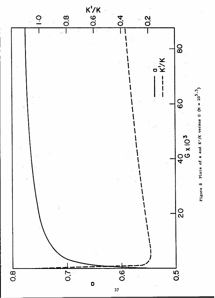
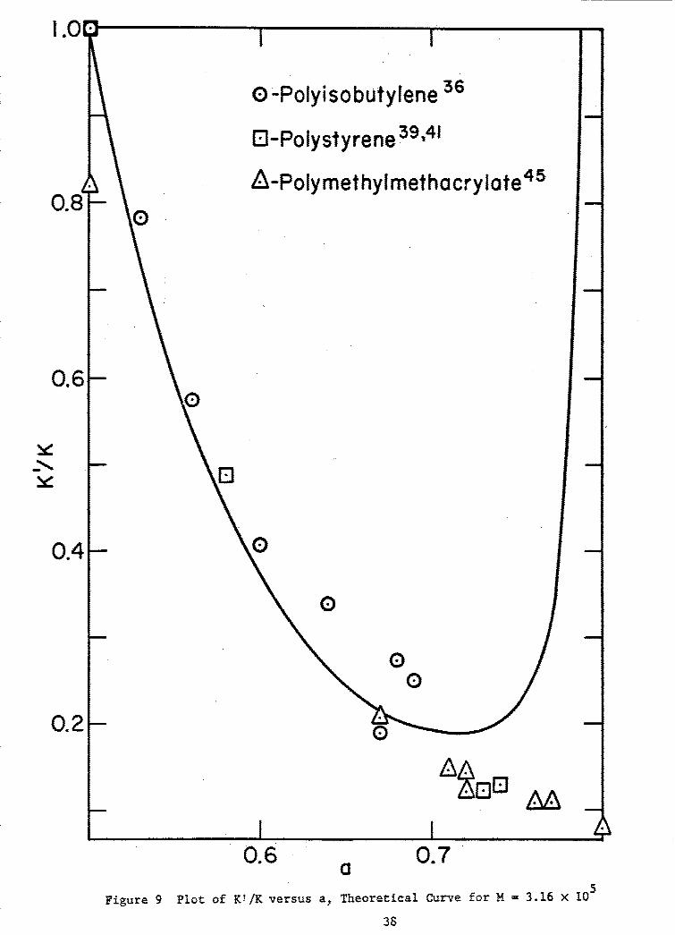
In Figs. 8 and 9, plots of a and V/K versus G and a plot ofKV/K versus a, respectively, are given. The latter curve retains noparameters of the theoretical relationships employed in its construction,other than K whose value for each of a number of polymers, ignoring possiblespecific solvent effects (see preceding section) may be regarded as a fairlywell known quantity. We have accordingly included in Fig. 9 for comparisonsome experimental values available from the literature.
From the plots of Figs. 7, 8 and 9 a number of interesting features,borne out for the most part by experimental data, are evident. in thetheoretical log [(i] versus log M plots of Fig. 7, for example, we note thatthe spacing of the parametric curves is not in linear proportion to the valuesof the interaction quantity G (see Eq. (32)) to which they refer. The effectis more pronounced in the plot of a versus G in Fig. 8, which in additionto exhibiting the increase in a with solvent power of the medium experimen-tally observed, predicts a rapid initial increase of the viscosity-molecularweight exponent, followed by a gradual asymptotic approach to the limitingvalue required by theory, 0.8, with increasing G. If the G value character-istic of some arbitrarily selected polymer-solvent pair is regarded as arandom quantity, uniformly distributed within observable limits, it is verylikely that the corresponding a value for the system will fall withinnarrowly defined limits (about-0.72-0.77). Whatever the basic origin ofthis effect, it is interesting to note that the predictions of theory inthis instance are supported by experimental evidence, i.e., the preponderanceof reported a values in the region described, and, perhaps more significantly,the paucity of observed values in the range 0.5 < a < 0.7.
We note finally in Fig. a that theory predicts a decrease in K'with increasing a over most of the range of polymer-solvent interactionencountered, and that qualitatively, at least, the effect is in accord with,experimental observations.
b. Calculation of the constants K' and a. In their recentpublication, Kawai and Naito suggest a "one point" method for the estimationof the Mark-Howink viscosity-molecular weight relationship appropriate to aparticular polymer-solvent pair of interest. The calculation requires aknowledge of the molecular weight of a single sample (preferably of minimalheterogeneity and lying about in the middle of the molecular weight range ofinterest) and the intrinsic viscosity of this sample in the solvent chosen,together with extensive [I]-M data for the same polymer dissolved in someother solvent. In accordance with the relationships presented earlier, weshall describe a similar, and perhaps more direct, procedure for carryingout this calculation.
If a number of values of [-q] and M are known for some polymer-solvent pairs, the constant K (Eq. (33)) for the polymer at the correspondingtemperature may be evaluated by the graphical procedure described in anearlier section. Ignoring possible specific effects, the value of K soestablished is, in accordance with theory, also applicable to the samepolymer dissolved in other media. Thus, insertion of this K value, togetherwith a single set of [TI-M values for the solvent of interest, in Eq. (30)permits evaluation of the expansion parameter a appropriate to the new system.
36
K'/K
coa
0 0
(03I C,
-0
d d37I
I.01
o -Polyisobutylene 3 6
O-Polystyrene 3 9 ,4z
0.8 A-Polymethylmethacrylate4 5
0.6-
0
0.4- 0
0
10
0.2- 0
0.6 a 0.7
Figure 9 Plot of K!/K versus a, Theoretical Curve for M = 3.16 x 10O
3S
From a, the slope of the tangent line to the theoretical [11]-M curve,
which we have interpreted as the Mark-Howink exponent a, may be computedin accordance with Eq. (35). The companion constant K' is obtainable fromEq. (36),utilizing previously determined values of K, a, C and M derivedfrom data on the single sample studied.
The viscosity-molecular weight relationship calculated in themanner described should provide a satisfactory representation over a rangeof molecular weights not differing greatly from that of the sample used inits construction. The validity of the values deduced for K' and a, restsprimarily upon the validity of the single set of [71]-M data utilized; thegeneral theoretical relationships assumed serve only as a means of intro-ducing a perturbation for variations in M from the assigned value. The useof average values of the viscosity constants (the logarithmic mean in thecase of K') derived from data on two or more fractions would, of course,increase the reliability of the relationship.
The viscosity-molecular weight relationship for a given polymer-solvent pair may also be estimated by another "one point" method which doesnot require viscometric data on a reference system. According to the theory4 1'
4 2
of intermolecular interactions advanced by Flory and co-workers, the expansionfactor a is related to the second virial coefficient A2 which appears in theseries expansion of the reduced osmotic pressure 3T/c.
g/c = RT[l/M + A2 c + .. .1 (37)
where c is polymer concentration and R is the gas constant, in accordancewith the expression
ln [1 + (Tl/2/2) (o2 - 1)] = (270/25/2 N) (ApM/[r]) (38)
Here, 0 is the viscosity constant appearing in Eq.(30) and N is Avogadro'snumber. Thus, a single set of the quantities M, [TI] and A2 for a givenpolymer-solvent pair suffices to establish the associated value of aappearing in Eq. (38). Once a is known, K may be computed from Eq. (30)and the constants K' and a may be evaluated in the manner described in thepreceding "one point" method. It should be noted, however, that in thepresent procedure, theory plays a somewhat more dominant role in assigningthe Mark-Howink constants.
5. The [n]-M relationship at low molecular weight. In thepreceding sections we have demonstrated the general compatibility of thetheoretical relationships(30) and(32) with the semi-empirical Mark-Howinkequation, applicable to high molecular weight polymers over a restrictedrange in M. We may conclude that the apparent linearity of log [r]-log Mplots experimentally observed in this region arises from the insensitivityof the derivative d ln U3 /d ln M, an effect which seems to be adequatelyaccounted for by the theory presented.
39
Some 4 5 1 4 7 1 4a polymer-solvent systems have been investigated inwhich viscometric measurements extended to the low molecular weight regionindicate the need for two equations of the Mark-Howink form in order tosatisfactorily represent the data. One of the relationships applies to thehigh molecular weight region, in accordance with the customary representa-tion, the other, of lesser slope, to the region of low molecular weights,usually less than about 30-50,000. On a logarithmic plot, the two linesintersect, forming an apparent "break point" in the [i]-M plots. Closeinspection of the data obtained for such systems shows that the log []l-log M relationship may in fact be equally well described by a smooth curve.Thus, by this interpretation, the representation by two intersecting lineswould appear to be merely a convenient means of expressing the data withinexperimental error.
According to the theoretical relationships presented here, theslope of the ln [I]- ln M curve should decrease monotonically with decreasingM, and, regardless of G, should attain at sufficiently low molecular weighta value experimentally indistinguishable from the characteristic 0.5 foundfor e-solvent mixtures over the entire range of M. This conclusion has beenreached by Rossi 35 et al, in whose publication an experimental verificationis presented fr polystyrene-toluene solutions.
The degree to which the theoretical curves fit experimental dataover a range of M in which d ln [i]/d ln M approaches one-half has beenexamined by Fox and Flory for polyisobutylene systems - e. The agreement inthese cases is rather good.
D. Summary and Conclusions
Zn this report we have outlined and discussed the progress todate on an experimental program designed to further our understanding ofthe specific effects of solvents on the e-point dimensions of polymerchains. Accurate 8-temperatures for the system selected in our initialwork should be established in the near future, at which time an extensiveinvestigation of the molecular dimensions of polystyrene in these 8-solventswill be undertaken. We have in mind extending our general methods to otherpolymer-solvent systems at a later date.
Many aspects of the problem of the specific effect of solventson chain dimensions are also amenable to theoretical treatment. In thisconnection, we have included in our report a draft of a manuscript which,in more general terms, deals with the viscometric behavior of polymersolutions, and which presents a re-interpretation of current polymer theoryin light of the possible influence of specific solvent effects.
We are also presently engaged in another theoretical investigationon the temperature dependence of the intrinsic viscosity, and hence moleculardimensions, in the vicinity of the 8-temperature.
40

III. Light Scattering Photometer - G. C. Berry, E. F. Casassa, D. J. Plazek
A. Introduction
A precision light scattering photometer has been designed andconstructed. The instrument is primarily intended to provide accuratemeasurements of the relative scattering from polymer solutions as a functionof angle and temperature. The design is such, however, that the instrumentcan also be used to measure absolute scattering. The optical design issimilar in principle to that described by McIntyre and Doderer 9 , and themechanical arrangement includes many features described by Katz 50 . Ahighly collimated monochromatic beam is split and then focused in a lightscattering cell and on a monitoring photomultiplier. The scattered lightis detected by a second photomultiplier which "sees" the scattering volumein the cell through a suitable optical system. The ratio of the two photo-currents generated in this manner is measured in a bridge circuit. Thismethod tends to eliminate the effect of lamp intensity fluctuations on themeasured response due to scattered light. The following report is adescription of the mechanical, optical and electronic design of thephotometer.
B. Apparatus
1. General description. Fig.I0 is a schematic drawing of theinstrument and associated equipment. Since the details of the constructionare available in a set of mechanical drawings, it is sufficient here topoint out the major components in the instrument. These consist of separatehousings for a lamp; for a set of monochromatic filters; for a mechanicalbeam chopper; for a set of neutral filters, beam splitter, and monitoringphotomultiplier; and for the detector photomultiplier. The last unitmounted on a goniometer permits accurate determination of scattering as afunction of angle. The sample cell is placed at the center of the
.goniometer either on an open pedestal or in an enclosed thermostat. Themechanical construction is such that all of the optical parts may beindividually adjusted, as required for the optical alignment. The entireunit is sturdily constructed to eliminate difficulties from vibration orunintentional mechanical shocks.
A model NBS Brinkman-Haake thermostat is used as the water bathand pump to supply the thermostating liquid to the cell thermostat. Thisliquid is circulated between the double walls of the thermostat and thuscontrols the temperature of a liquid bath surrounding the sample.
2. Optical design. Fig. 11 is a schematic diagram of the opticalsystem of the instrument. The light source is a mercury vapor lamp, withthe arc aligned perpendicular to the optical axis. Two such lamps areconsidered below. The source is located approximately at the focal pointof lens L, (the characteristics of the optical parts are given in Table VI).
41

00 0
0 Cd
uH
0s 4.
Irf 0
xsi 0
C! iI=
Hs 04 =00
0c W
P4- 0. t
IP-
CLC
Q 0 aP4H
-
is 0MI0
Ci isH 4i

'-4n
CI
r~ra
-44
14
en 44
434

Table VI
Optical Parts of the Photometer
Part Description
LI, L2 35 mm projection lens, 7 in f.l.; Anastigmat F/3.6 coated lens
L3 44 mm dia; 189 mm f.l.; coated achromatic lens
L4 18 mm dia; 39 mm f.l.; coated achromatic lens
Ls 29 mm dia; 40 mm f.l.; lens
A 2 3/8" dia. heat absorbing glass
G, Corning glass filters 3484, 5120
G2 Corning glass filters 3484, 4303, 5120
B Corning glass filters 3309, 5113
N, 2" dia. Series VII metallic neutral filter (Tiffen OpticalCo.), trans 1/8
N2 2" dia. Series VII metallic neutral filter (Tiffen Optical
Co.), trans 1/32
N3 Neutral filters, Phoenix Co., trans 1/2
N4 Neutral filters, Phoenix Co., trans 1/4
N5 Neutral filters, Phoenix Co., trans 1/8
Ne Neutral filters, Phoenix Co., trans 1/16
N7 Schott neutral filters, (Fish-Schurman Co.), NG 4; trans 1/10
N8 Schott neutral filters, (Fish-Schurman Co.), NG 4; trans 1/10
N9 Schott neutral filters, (Fish-Schurman Co.), NG 5; trans 1/3
N1 0 Schott neutral filters, (Fish-Schurman Co.,), NG 11; trans 1/2
N1 1 Neutral filter, trans about 1/20
Sh 4 Prontor II shutter
P1, P2 1 1/2" dia., 3.5 mm thick polarizers, Polaroid HN22C, SpC, FGE Glass
M, D DuMont K1780 photomultiplier tubes
Wi 32 mm dia.
W2 Cut from 100 mm ID pyrex tube
Pr1 Silvered right angle prism; 34 mm width, 45 mm hypotenuse, 32 mm side
Pr 2 1 1/4" glass cube (no = 1.508) fabricated from two 450 right angle
prisms with cement of refractive index about 1.495 (Tiffen
Optical Co.)
Source 200/250 volts, 250 watt ME/D box lamp
Source HIOO-A4 General Electric mercury vapor lamp
44

Lens L, receives light through a large slit So and a heat absorbingfilter A. The essentially parallel light from L, passes through one ofthe three monochromatic filters G1 , G2 or B. N, and N2 are removableneutral filters; Sh, is a sliding shutter. Lens L2 is identical to L1 ,and may be moved independently of L1 . The position of L2 is adjustedso that the aperture S2 is in the focal plane of L2 by focusing an imageof the source at S 2 . The position of S1 is adjusted so that its image is
focused in the cell. Lens L3 is adjusted so that S2 is in its focal
plane. This arrangement gives a highly collimated beam of light from
the exit of L3 .
The beam splitting prism is a glass tube constructed from two
triangular prisms cemented along the diagonal faces. The refractive index
of the cement is close to that of the glass so that the primary beam
suffers only negligible polarization and attenuation at the interface.
The opposite sides of the cube are ground parallel and polished.
The lens L 5 is chosen to make the optical path length from L3to the monitor photomultiplier M nearly identical to that from L3 to the
cell. Thus, a uniformly irradiant image of S, is focused both in the celland on M. A second prism, Pr 2 merely turns the monitor beam downward
through 900 into M to maintain compact dimensions in the unit. Other
components in the maini-filter box include the removable neutral filters
for the primary beam, N3 to N6 , and for the monitor beam, N7 to N 10 .
Sh 2 is a sliding shutter and W, is a plane glass window to keep dust out
of the housing. S3 and S4 are stray light slits, made slightly largerthan the primary beam at their respective positions.
The cell is normally enclosed in a thermostat with a clear glass
W 2 and a neutral filter Ni1 as plane entrance and exit windows respectivelyfor the primary beam. The neutral filter (of about 5 percent transmission)
serves to reduce back reflection of the incident beam into the cell from
the glass-air interface by a factor of 400. Without this attenuation the
back reflection of about 5% of the incident beam would produce scattering
in the sense opposite from the incident beam sufficient to falsify
seriously angular dependence measurements on very large molecules 5 2 . The
scattering volume is viewed through a curved window W3 , ground and polished
on the outside surface. The light scattering cell may be cylindrical in
shape, such as that used in the Brice-Phoenix photometer, or conical, a
form which helps to reduce reflections5 3 . In the latter case, the ther-
mostat liquid in which the cell is immersed must have a refractive index
rather close to that of the scattering liquid if undesirable refractions
are to be avoided. The detector optics follow a design given by
Kushner 4 . Slits S5 and S6 are placed in the focal and image planes,
respectively, of lens L 4 . The detector photomultiplier, D, views the
light passing slit Se. Sh3 is a camera shutter and 0 is an opal glass
diffuser which is in the line of view only when the detector is viewing
the primary beam directly.
The removable polarizers, P1 and P2 , are mounted so as to be
easily rotated precisely through 90'. They have a resolving power of 10
seconds of arc.
45
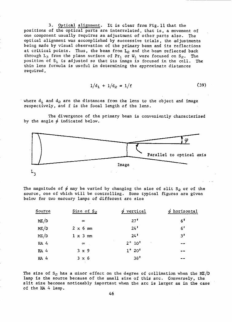
3. Optical alignment. It is clear from Fig. il that thepositions of the optical parts are interrelated, that is, a movement ofone component usually requires an adjustment of other parts also. Theoptical alignment was accomplished by successive trials, the adjustmentsbeing made by visual observation of the primary beam and its reflectionsat critical points. Thus, the beam from L2 and the beam reflected backthrough L3 from the plane surface of Pri or W1 were focused on S2 . Theposition of S, is adjusted so that its image is focused in the cell. Thethin lens formula is useful in determining the approximate distancesrequired,
1/d1 + l/d 2 = 1/f (39)
where d, and d2 are the distances from the lens to the object and imagerespectively, and f is the focal length of the lens.
The divergence of the primary beam is conveniently characterizedby the angle $ indicated below.
Parallel to optical axis
Image
L3
The magnitude of $ may be varied by changing the size of slit S2 or of thesource, one of which will be controlling. Some typical figures are givenbelow for two mercury lamps of different arc size
Source Size of S2 $ vertical $ horizontal
ME/D CO 27' 61
ME/D 2 x 6 mm 24' 6'
ME/D 1 x 3 mm 24t 3V
HA 4 1 201 --
HA 4 3 x 9 1i20' --
HA4 3x6 38' --
The size of S2 has a minor effect on the degree of collimation when the ME/Dlamp is the source because of the small size of this arc. Conversely, theslit size becomes noticeably important when the arc is larger as in the caseof the HA 4 lamp.
46

The monitor system is similarly aligned by visual means. Theprism Pr 2 is placed so that light falls on the central part of M, and thenLS and NM are adjusted until the image of S, is focused on M.
The alignment of the detecting system involves two adjustmentsafter the photomultiplier housing has been placed on the optical axis ofthe primary beam. S5 is placed in the focal plane of L& by visuallyfocusing a beam of parallel light on SS. Placement of Sa in the image planeof L, requires a scattering source located in the position of the cell.Thus, the image of an opal diffuser at the cell position was focused on S6by movement of the system L4 :S 5 , with the distance between the latter twoelements fixed. The distances from the cell to L4 and from L4 to S5 and S6can be estimated by Eq. (39) and the lens focal length, but visual adjust-ment is necessary unless the nodal points of L4 are determined and used todefine the distances in Eq. (39), since L4 is not thin compared to d2 and f.The observation may be made by viewing the image on a thin paper screen inthe plane of the slit.
For a given lens and scattering volume, the angular resolution ofthe detecting system is determined by slit S5 or the lens diameter, one ofwhich will be controlling. Fig. 12 shows the angle *, defined as thelimiting plane angle of acceptance. No ray incident on L4 making an anglewith the axis of the receiver greater than * can pass through S5.
The angle * may be estimated by assuming a uniform scatteringvolume, and refraction at the air-glass interface of the thermostat. There
Sresults
0/2f if 9 < f(D + y)/dltan i• = (40)(D + y)/2d3 if 2 > f(D + y)/d 1
ýTT
Cell L4 S5 S6 Pah cacubeImage .
Figure 12 Detector Optics
47

Refraction can be accounted for approximately by replacing * with ' =/n,where n is the liquid refractive index. The distance y is fixed by thedimensions of S6 or the scattering volume in the cell. Since it is desir-able not to have the detector photomultiplier see past the edges of thebeam, S6 is made to be the controlling element. In particular y', thesize of S6, is given approximately by
y= nyf/(d1 - f) (41)
It is important to note in Eq. (40) that if I is small enough, the angleof acceptance becomes independent of the size of the scattering volume.
These detector optics and the highly collimated primary beammake it possible to use the photometer as an absolute instrument if desired.Kushner 5 4 has shown that the scattering volume defined by these optics iseasily calculated from the geometric parameters of the system. This, com-bined with the observations of Hermans and Levinson5 5 concerning therefraction corrections applicable when the detector does not see past theedges of the scattering volume, allows a direct correlation between theRayleigh scattering factor and the ratio of the instrument response to thelight scattered at 90* and to a section of the primary beam attenuated bya dense filter of accurately known transmittance.
The height of the scattering volume is limited by the entrancewindow to the thermostat. The width and depth of the scattering volume,that is, its dimensions parallel and perpendicular to the axis of theprimary beam in a horizontal plane, are limited by two criteria. Thevolume must be small enough so that the detector will not see scatteringand reflections from the entrance and exit positions on the cell wall atany angle of observation and so that deviations from uniform irradiancein the scattering volume are negligible. At present the apparatus includesa 1 x 3 mm slit at S5 and a 1.8 x 1.8 mm slit at Se with Se 209 mm from thecenter of the cell. These dimensions are critical since a change in onewithout a change in others could result in the detector photomultiplierseeing past the edges of the scattering volume or in an increased angularacceptance. This arrangement sets the angular acceptance, fS, at about2.70 in the vertical and i° in the horizontal directions. These angleswould both be 30 in the absence of slit S 5 .
4. Electrical design. The photomultiplier circuit is shownschematically in Fig.13. The dynode resistors (not shown) are sealedinto the tube base by the manufacturer. Resistors R5 prevent formationof a space charge about the anode. Resistor R6 allows the monitoringphotomultiplier tube to be operated at a lower voltage than the detectortube to reduce its noise contribution. This can be done since obtainingsufficient light at the monitor tube is never a problem. The DC powersupply (John Fluke, Mfg. Co., Model 405) provides voltages adjustablecontinuously from 600 to 3000 volts, regulated to within 0.1% maximumdeviation for a 20% change in line voltage, with less than 0.005% drift
per hour.
48

S-------"-E Power - E----
R supply
•R5 R5
•-- Anod Anode
SwI Sw2
Sw
3
R ~R 7C ,I
C l
H = 100 K
+ 200 V Tube No. 5963 R3 = 10 R,
R4 = 22 K
R 5 = 100 K
S••R3 R6 =3.5M
C1 = 18 to 2 00 i4f
RR Tuned Sw1, Sw2 JBT#S52
S-LlVoitmeter Sw1, JBT#ST52P
-"MD,. duMont K1780
T, T, Triad No. G-22
Figure 13 Electronic Circuit
49
The anode photocurrents are sent to ground potential through tworesistors, RH and R2 (normally, R2 = RH). The resistors are 10-turn model7601 Beckman "Helipots." These potentiometers are linear to within 0.015%for readings greater than 20% of full scale, and to within 0.025% forreadings greater than 5% of full scale.
The switching arrangement shown allows one to observe the voltageimpressed on either RH or R2 , or the difference between the voltagesimpressed on R, and R2 . The variable capacitors C, are used to shift therelative phase of the voltages in the bridge to that necessary for exactcancellation (180°). Although the photocurrents are produced in exactlythis relationship, reactances in the circuit are sufficient to requirecompensation. The details of this adjustment are discussed below.
The signal from the bridge (points I and 2, Fig. 13) is sent tothe grids of an impedance matching dual cathode-follower tube, type 5963.The plate voltage for this tube may be supplied by any regulated powersupply, or by batteries. The signal from the cathode follower goes to theprimary winding of an isolation step-up transformer (4:1) so that thedifferential signal is transformed into a single ended signal. This signalis then measured on a voltmeter tuned to the chopper frequency. A Hewlett-Packard model 302-A wave analyzer serves this purpose.
The wave analyzer utilizes the heterodyne principle. The incomingsignal is mixed with a signal from an internal oscillator to give a signalof a fixed difference (or heterodyne) frequency to which a selectiveamplifier is tuned. The selective amplifier includes a crystal filter circuitof very narrow bandpass characteristic: the response attenuated by 3db at+ 3 cycles and by 80db at + 70 cycles. The light beam is chopped mechanicallyso that the desired signal has a frequency of 450 cps. The 450 cps frequencyis chosen so that the 60 cps pickup or its harmonics will be effectivelyattenuated. There is no observable signal from this source when the volt-meter is tuned to 450 cps. The signal also has a strong component at 120cps (and harmonics) since the lamp is operated from a 60 cps power supply.An alternative to this would be to operate the lamp from a DC power supply,chopping the beam at 450 cps. This should increase the RMS signal measuredon the tuned voltmeter. The lamp is presently being operated from an ACsupply because the high current regulated supply required for DC operationis not readily available.
5. Electronic performance. The purpose of the bridge circuit isto reduce so far as possible the effect of lamp intensity fluctuations onmeasurement of the response due to scattering and to allow more accuratedeterminations of the relative photocurrent than might be possible fromdirect reading of a single phototube signal on a meter. If both photo tubesrespond identically to fluctuations in the intensity or position of the arc,the ultimate resolution of the bridge is governed by the noise generated inthe photomultipliers and by the resolution of the tuned voltmeter. Thephotomultiplier noise far exceeds that generated elsewhere in the circuit(amplifier noise, Johnson noise, 60 cps pickup, etc.) and can be estimatedby the relationship
5 6
50

(S/N) 2 = ip 2 /2e&f(it + ip) (42)
where S/N is the signal to noise ratio, i and it are the photo currentand thermonic emission at the cathode, respectively, e is the electroniccharge, and Af the bandwidth of the measuring instrument. There are twocontributions to the noise given by Eq. (42): the thermonic emission andthe shot noise arising from the statistical natureaE the photo emissionprocess. Eq. (42) predicts that the S/N ratio will vary with the squareroot of i for large photocurrents (intense light flux), and with ip forvery small photocurrents.
The percentage error in the bridge balance can be obtained from
R .I . _ I V +( 4 3 )R2 M
where ID and IM are the detector and monitor photocurrents, respectively,and vD is the voltage impressed on R2 , of the order of I my. The un-
certainty in the signal at the null balance of the bridge is given by 6V.
If the noise from the phototubes were sufficiently small, 6V would be
determined by the resolution of the measuring instrument, of the order
of 1 . volt for the tuned voltmeter. In fact, if the phototube impressed
some constant voltage across RH and R2 , the voltmeter resolution would
still determine WV. There are, however, low-frequency fluctuations in
the noise level which are partially damped out by the meter, but which
still make it difficult to determine the exact null point. Fig.
illustrates this problem schematically. The voltage across the bridge
is plotted as a function of the resistor ratio R2 /R 2 . The desired null
balance occurs when RI/R 2 = ID/IM. The amplitude fluctuations in the
noise level, however, allow one to come only within 5V of the desired
balance.
V D
N ,L..
>I
R /R
Figure 14 Effect of bloise on Rull Sensitivity
51
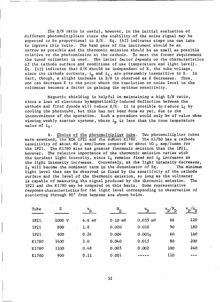
The S/N ratio is useful, however, in the initial evaluation ofdifferent photomultipliers since the stability of the noise signal may beexpected to be proportional to S/N. Eq. (42) indicates steps one can taketo improve this ratio. The band pass of the instrument should be asnarrow as possible and the thermonic emission should be as small as possiblerelative to the photoemission at the cathode. To meet the former requirementthe tuned voltmeter is used. The latter factor depends on the characteristicsof the cathode surface and conditions of use (temperature and light level).Eq. (42) indicates that S/N should be independent of E, the tube voltage,since the cathode currents, ip and it, are presumably insensitive to E. Infact, though, a slight increase in S/N is observed as E decreases. Thus,one can decrease E to the point where the resolution or noise level in thevoltmeter becomes a factor in gaining the optimum sensitivity.
Magnetic shielding is helpful in maintaining a high S/N ratio,since a loss of electrons bymagnetically induced deflection between thecathode and first dynode will reduce S/N. It is possible to reduce it bycooling the phototube, but this has not been done as yet, due to theinconvenience of the operation. Such a procedure would only be of value whenviewing weakly scatter systems, where ip is less than the room temperaturevalue of it.
6. Choice of the photomultiplier tube. Two photomultiplier tubeswere examined, the RCA IP21 and the duMont K1780. The K1780 has a cathodesensitivity of about 60 p amp/lumen compared to about 40 p. amp/lumen forthe 1P21. The K1780 also has greater thermonic emission than the 1P21,however. The relative importance of the thermonic emission varies withthe incident light intensity, since it remains fixed and ip increases asthe light intensity increases. Conversely, as the light intensity decreases,it will become the dominant term in the denominator of Eq. The minimumlight level that can be observed is fixed by the sensitivity of the cathodesurface and the level of the thermonic emission, so long as the voltmeteris capable of measuring the signal produced by the thermonic emission. TheIP21 and the K1780 may be compared on this basis. Some representativeresponse characteristics for the light level corresponding to observation ofscattering through 90* from benzene are shown below.
Tube E vD ND nD vD/ND vD/nD
IP21 1000 V 6.6 mV 0.10 mV 0.035 mV 66 220
IP21 800 1.8 0.020 0.010 90 180
1P21 600 0.24 0.004 0.0015 60 160
K1780 1400 3.0 0.040 0.015 80 200
K1780 1100 0.48 0.005 0.002 100 240
K1780 900 0.11 0.001 110 ---
52
The response is expressed as the voltage impressed across RH, vD being theRMS contribution from the photocurrent, and ND and nD the total tube noiseand the thermonic component, respectively. The ratio vD/nD is approximatelyindependent of E, as epxected, and indicates that the weakest light levelfor which the photomultiplier will give a usable signal is about the samefor both tubes. The lower limit of detection, fixed by the cathode sensi-tivity and the thermonic emission, is about 200 times less than the scatteringobserved from benzene at 900 with the ME/D lamp as the source and bothphototubes at room temperature. In addition, the low frequency fluctuationsin the phototube noise are less severe with the K1780. Thus, the presentapparatus employs the K1780 for both monitor and detector.
7. Choice of the light source. Two mercury vapor lamps wereexamined: the 250 watt Mazda (Metropolitan Vickers) NE/D and the 100 wattHA4 (General Electric). The former source produces a primary beam about12 times more intense than the latter if the comparison is made for beamscollimated such that 9 is about 30' in the vertical direction. Unfortunately,however, the ME/D also exhibits much greater fluctuations in the arc positionand intensity than does the HA4, and apparently has a relatively shortlifetime (average lifetime given as 500 hr. in lamp specifications). Someof the loss in intensity incurred when using the HA4 can be recovered bysacrifice in beam collimation. Thus, the beam intensity can be increasedby a factor of two if 0 is allowed to change from 38'-to 2010' in thevertical direction. The Me/D is used in the present apparatus since itwill allow measurements of scattering from materials which give only onehundredth the scatter from benzene at 90*. If the use of the instrumentis to be confined to strongly scattering polymer solutions, however, itappears the HA4 would be a more suitable choice in view of its longerlifetime and better stability.
8. Performance. Several aspects of the performance have alreadybeen discussed, including the divergence of the primary beam, the angularacceptance of the detector, and the phototube behavior. In this sectionsome measurements of a null balance and its behavior will be considered.
The bridge circuit effectively removes the effects of long termdrifts in the lamp intensity, but the effect of rapid fluctuations in theintensity and position of the arc are uncertain. This effect has beenminimized by keeping the optical path lengths from L3 to the cell and tothe monitor phototube as nearly alike as possible, but complete compensationhas probably not been accomplished. Further study is necessary to clarifythis point. In any case, the effect is now small enough so that it consti-tutes no severe problem in attaining an accurate null point. Another sourceof error is the effect of temperature on the beam splitter, PrI. The amountof light reflected to the monitor may vary by as much as 5% per 1C shift inthe prism temperature. This is apparently due to the closeness of therefractive indices of the glass and cement. A slight shift in either causedby the change in temperature is sufficient to cause a marked change in theamount of light reflected from the interface, since this depends on thesquare of the difference of the refractive indices. This drift is unfortunatebut is no real problem since room temperature variations are negligible duringany single series of measurements, and the ratio of the intensities determinedat any two angles is independent of this effect.
53

The table below indicates the reproducibility of the nullbalance readings. These readings were determined with E = 1100 volts for themagnetically shielded detector photomultiplier, and with the ME/D lamp as thelight source.
Root-mean-squaredeviation from
Source Photocurrent mean reading
Benzene 900 scatter 0.0050% amp 0.3%
Attenuated benzene scatter 0.00060 1 %
Attenuated benzene scatter 0.00012 3 %
Attenuated benzene scatter 0.00007 8 %
These figures indicate satisfactory performance of the bridge circuit.
The bridge circuit includes two variable capacitors which haveimpedance much greater than the helipots. As mentioned above, these arenecessary to balance the out-of-phase portion of the signal. A completenetwork analysis of the bridge has not been done, but the results for somecases included in Appendix II, are useful at this point. It is shown therethat if the out-of-phase imbalance is caused by some capacitive shunt toground, then it may be corrected by suitable adjustment capacitors shuntedacross the phototubes. The calculation indicates that this setting shouldbe independent of the ratio R1 /R 2 , i.e. of the helipot setting. Anotherlimiting case occurs when only inductance in the helipots is of importance.This result indicates that such an effect ought to be corrected forautomatically, since the correction requires the ratio of the two induc-tances to vary as the ratio R1 /R 2 and this should be close to the actualsituation in the helipots.
In practice, one adjusts the capacitors so that the minimumvoltage at null balance is equal to that impressed on the bridge by thephototube noise (this can be determined at 500 cps where the main signalis greatly attenuated and the signal left is due to the phototube noise).This adjustment increases the sharpness of the null, although it has anegligible effect on the exact position of the null. The capacitoradjustment is not independent of the helipot setting, however, suggestingthat there must be sources of the phase imbalance other than those includedin the simplified network analyses we have worked out. The observationthat the value of RI/R 2 is only negligibly affected by the capacitor ad-justment is taken as an indication that the resistor ratio is truly theratio of the photocurrents, at least within the experimental error ofdetermining R/.
54

C. Conclusion
The light scattering photometer described is capable ofdetermining the relative scattering to within 0.3% from materials rangingin scattering power from benzene to strongly scattering polymer solutions.In addition, depolarization measurements and the scattering from much moreweakly scattering liquids may be determined with some loss in precision.The scattering volume is illuminated by a highly collimated beam of light,and the detector has a low angular acceptance, making the instrument usefulwhere high angular resolution is necessary. The temperature of thescattering volume may be held constant over a wide range.
D. Future Work
The completion of the light scattering photometer brings theimmediate project to a conclusion, but since the instrument was constructedwith certain studies in mind, a brief note of some anticipated investigationsis pertinent. In general terms, the future work will be concerned withmeasurements on the thermodynamic and configurational properties of poly-mers in solution for comparison with theoretical predictions. In particular,the effect of molecular weight, temperature, and molecular weight distributionon the second virial coefficient and on the molecular configuration willbe skdiedThese investigations will be made on polymers of various structures, i.e.,flexible linear and branched chains, stereoregular molecules, and stiffchains. It is expected that these data will also be useful in suggestingpossible directions for new developments.
IV. Viscosity - Molecular Weight Relationship for Poly-(Vinyl Acetate) -
R. E. Kerwin and H. Nakayasu
A. Introduction
The intrinsic viscosity - molecular weight relationship forlinear Poly-(vinyl acetate) in methyl ethyl ketone has been studied by anumber of investigators57- 0. All of these studies deal principally withpolymers of molecular weight higher than 100,000 with a few measurementsof lower molecular weight material covered in references 59 and 60. Inconnection with other work undertaken in this laboratory, it has becomenecessary to know which, if any, of these published relationships remainvalid in the region of lower molecular weights. Accordingly, we havecarried out viscosity and light scattering measurements on this systemusing polymer fractions of molecular weight from 6,000 to 30,000.
55
B. Experimental
The polymer labeled PD-2 in Table VII is a linear, low conversion(14.8%), low molecular weight poly-(vinyl acetate) prepared in bulk at 300Cby photo-polymerization of vinyl acetate with t,a'-azodiisobutyronitrilephotosensitizer (.289 moles/liter) and acetaldehyde chain transfer agent(.233 moles/mole of monomer; chain transfer constant C = 0.02). Thismaterial was fractionated at 30* from a 2% solution in benzene usingligroin (solvent naphtha) as the non-solvent&±. Polymer RKI was preparedsimilarly except that chloroform was used as chain transfer agent (1.15moles/mole of monomer; C = 0.015) and the polymerization proceeded to 36%conversion. This polymer was fractionated at 28CC from a 4.4% solutionin toluene using n-hexene as non-solvent. The high chain transfer con-stants of these two chain transfer agents insured low molecular weightproducts.
The methyl ethyl ketone used as solvent in the viscosity andlight scattering measurements was purchased as reagent grade and furtherpurified by drying over "Drierite", distilling, and storing in darkbottles at OC.
The light scattering measurements were made at 250C with aBrice-Phoenix light scattering photometer and a cylindrical cell withflat entrance and exit windows. The apparatus was calibrated with respectto a 0.75% solution of "Cornell Polystyrene" in methyl ethyl ketone forwhich the absolute excess scattering at right angles iRayleigh's ratio)for unpolarized 5416A0 light was taken62 as 632 x 10 . Measurementswere made on the solvent and four concentrations of each fraction and atat least 7 angles including 450, 900 and 1350. These concentrations rangedfrom 0.7% to 2.0% for the highest molecular weight solutions and from 3.0%to 9.8% for the lowest molecular weight solutions. Fraction PD-2-12& wasmeasured in a small semi-octagonal cell since only 1.5 grams were available.All results were treated according to the method of Zimmi"s to determine theweight average molecular weight, k. Fig. 15, the Zimm plot for fractionPD-2-12A, serves as an illustration. The refractive index increment usedin these calculations was 0.080 cc/g, the value reported by Shultz5 7 andby Matsumoto and Ohyanagi•. The concentrations of all solutions weredetermined by weighing freeze-dried polymer directly into volumetricflasks and diluting to volume at known temperature. The glassware used tocontain or transfer the solutions for light scattering was rinsed in acetonedistilled to remove all traces of dust. The solutions were rendered dust-free by centrifuging for one hour at 14,000 RPM in a "Servall" SS-I centrifuge.
Viscosity measurements were carried out with a Cannon-Ubbelohdesemi-micro viscometer, model A 258. No kinetic energy correction was appliedto the data since the maximum correction factor, calculated from the dimen-sions of the viscometer and the solvent flow time, amounted to only 0.03%.
For polymer PD-2 four concentrations were measured for eachfraction, each being prepared separately to avoid dilution error in the
viscometer. The ranges of concentration employed were I to 3 g/lO0 cc.
for the highest [TI] and I to 10 g/lOO cc. for the lowest. Solutions were
56

Wa 0
<..
-4
04
4-3
'--..4
.4.
-4
0)
-ý4
t;t
L914
57
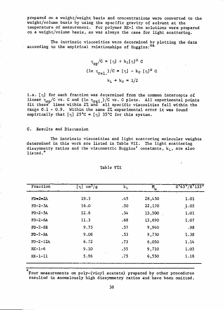
prepared on a weight/weight basis and concentrations were converted to theweight/volume basis by using the specific gravity of solvent at thetemperature of measurement. For polymer RK-l the solutions were preparedon a weight/volume basis, as was always the case for light scattering.
The intrinsic viscosities were determined by plotting the dataaccording to the empirical relationships of Huggins:64
sp /C = [rT] + kl[•] 2 C
(In rel. )/C = [T] - k 2 [•T] 2 C
k, + k2 = 1/2
i.e. [rj] for each fraction was determined from the common intercepts oflinear qsp/C vs. C and (ln Tlrel.)/C vs. C plots. All experimental pointsfit these lines within 2% and all specific viscosities fell within therange 0.1 - 0.9. Within the same 2% experimental error it was foundempirically that [TI] 25 0 C = [TI] 35CC for this system.
C. Results and Discussion
The intrinsic viscosities and light scattering molecular weightsdetermined in this work are listed in Table VII. The light scatteringdissymmetry ratios and the viscometric Huggins' constants, kj, are also1 is ted. *
Table VII
Fraction [k, cm3 /g kX R'45-/R' 1350
FD-2-2A 19.3 .45 28,430 1.01
PD-2-3A 16.0 .50 22,170 1.05
PD-2-SA 12.6 .54 15,500 1.01
PD-2-6A 11.3 .68 13,690 1.07
PD-2-8B 9.75 .57 9,940 .98
PD-2-9A 9.08 .53 9,730 1.38
PD-2-12A 6.72 .73 6,050 1.14
RK-1-6 9.10 .55 9,710 1.03
RK-1-11 5.96 .75 6,550 1.18
Four measurements on poly-(vinyl acetate) prepared by other proceduresresulted in anomalously high dissymmetry ratios and have been omitted.
58

These data are plotted with those from references 57-60 on theusual double logarithmic coordinates in Fig. 16. The published viscosity-molecular weight relations obtained in the earlier work are listed belowand the pertinent data are collected in Appendix III.
ShultzsT Log [(] -1.871 + 0.71 Log MW
Elias and Patate° Log [(] -1.377 + 0.62 Log Mw
Matsumoto and Ohyanagie 1 Log [(] -1.9706 + 0.71 Log Mw
The straight lines determined by the first two equations areshown in Fig. 14. The line corresponding to the equation of Matsumotoand Ohyanagi lies slightly below all of the existing data including theirown. A good fit to their data is given by a line of the same slope butwith K = 1.135 x 10⁻² instead of K = 1.07 x 10²'.
Shultz's equation was derived as the best fit to his data andthose of Howard whichtogether cover the molecular weight range from246,000 to 3,460,000. From the graph it may be readily seen that exceptfor the point for RK-1-11 the results of this present work agree within2% with the low molecular weight extrapolation of Shultz's line.
It is evident from the figure that the line corresponding tothe equation of Elias and Patat deviates by about 25% from the very lowmolecular weight data of this work and by about 15% from the very highmolecular weight data of Shultz. In addition to their light scatteringdata, which is presented in Fig. 16, Elias and Patat consideredsedimentation-diffusion molecular weight measurements for the range17,000 < Ms D < 1,200,000 in deriving their equation. Of their eightexperimental points for Mw from light scattering the lowest six agreewell with Shultz's line. Of the remaining two, one, the point forMw = 1.2 x 10⁶L majy be considered doubtful as the polymer was poorlyfractionated, Mw/Mn being listed by the authors as 3.00. -Light scatteringand sedimentation-diffusion molecular weights determined on duplicatesamples by Elias and Patat are in agreement within experimental error;hence it is the points at lower molecular weight, for which only sedimentation-diffusion data are available, which cause their divergence from other studies.
The data of Matsumoto and Ohyanagi fall 12% below Shultz's lineand generally below all previous data. There are two possible sources ofthis disparity, their use of whole polymer and their polymer preparativeprocedure. The authors themselves consider the fact that their polymer isnot fractionated and arrive at the conclusion that the measured viscosityfor their heterogeneous polymer (Mw/Mn - 2.00) should be 5% lower than [n]for a homogeneous fraction of the same Mw. (cf. Table VII and discussion,reference 60. It may be that their method of preparation of poly-(vinylacetate), involving as it does two precipitations in water and finallyboiling in water, brings about a significant amount of hydrolysis. Thiswould lead to the presence of species other than poly-(vinyl acetate) intheir solutions.
59
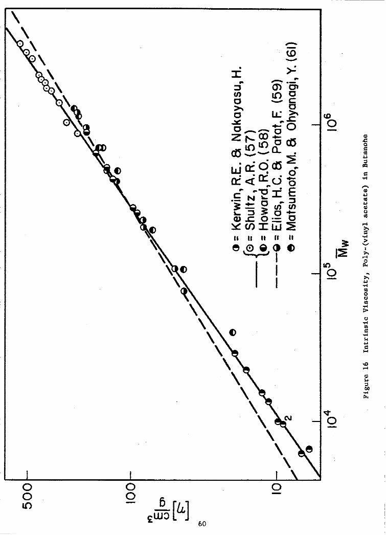
0*)0
0 -0 OD
to 01(2 too
0j * i (00
-I--tc -r
~ f- w 0 )-
v cO0 C'
I I I0 R-r4.
IIocQ)
0U
607
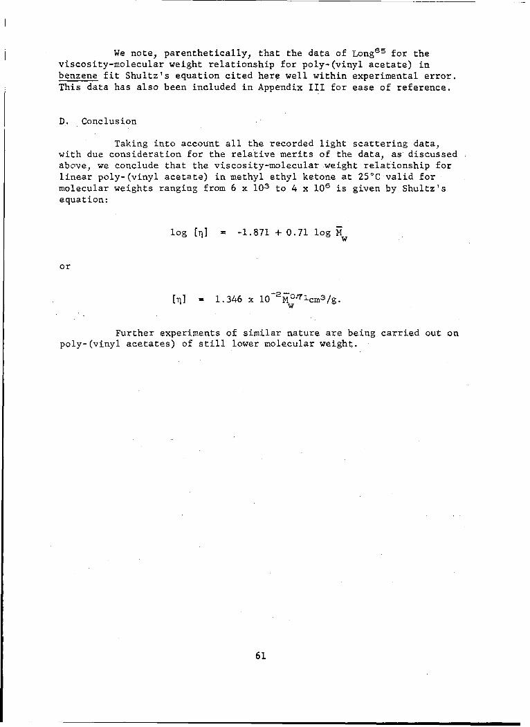
We note, parenthetically, that the data of Long 6 5 for theviscosity-molecular weight relationship for poly-(vinyl acetate) inbenzene fit Shultz's equation cited here well within experimental error.This data has also been included in Appendix III for ease of reference.
D. Conclusion
Taking into account all the recorded light scattering data,with due consideration for the relative merits of the data, as discussedabove, we conclude that the viscosity-molecular weight relationship forlinear poly-(vinyl acetate) in methyl ethyl ketone at 25'C valid formolecular weights ranging from 6 x 10³ to 4 x 10⁶ is given by Shultz'sequation:
log [O] = -1.871 + 0.71 logw
or
[r] = 1.346 x l0- 2M°o•cm3/g.w
Further experiments of similar nature are being carried out onpoly-(vinyl acetates) of still lower molecular weight.
61

Appendix I
Evaluation of Wu - Some details concerning the determinationof wu are noted here. In performing the integrations indicated in Eq. (39),we consider in turn each of the eight double integrals obtained in multi-plying the successive terms of w, as defined in Eq. (34), by f(x,u)f(y,u).The first four integrals turn out to be identical and expressible in termsof the forms
Sxi/2e-uxdx
and1
o x/2euXdx,
which upon integration by pa~ts yield expressions containing the irreducibleintegrals erf(uI/2) and e(u 2 ).
The last four double integrals in wu are more difficult toevaluate but happily are also identical, all being equivalent to
(x + y)1/2f(x,u)f(y,u)dxdy
o 0
After substitution of a new variable V = x + y and multiplication of thefactors in this integral, the evaluation of the resulting nine doubleintegrals proceeds as before to yield results again in terms of errorfunctions and e.
The final result, Eq. (40), was checked by expansion ofwuu'P 2 (u) in series. When terms in like powers of u were collected, theobvious requirements were met that coefficients of the terms in u0
through u3 vanish and that the coefficient of the UiL term be wo.
The integral E (x) - This function was apparently first tabulatedby Dawson in the interval 0 < x K 2; and the compilation was latercorrected and extended x = 4 for intervals of 0.01 by Terrill and Sweeney. 2 3
More recently tables have been publishedr of the related function
PXo X
e -x exp(t 2 )dt0
62
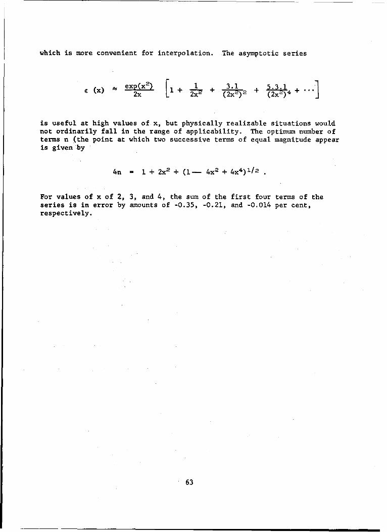
which is more convenient for interpolation. The asymptotic series
S(x) • exp(x 2 ) L i+ 3.1 + 5.3.1 12x 1+ +(2x-) 2 (2x-) 4 +.
is useful at high values of x, but physically realizable situations wouldnot ordinarily fall in the range of applicability. The optimum number ofterms n (the point at which two successive terms of equal magnitude appearis given by
4n 1 1 + 2x2 + (I1- 4x2 + 4x4)1/2
For values of x of 2, 3, and 4, the sum of the first four terms of theseries is in error by amounts of -0.35, -0.21, and -0.014 per cent,respectively.
63

Appendix II
The network analysis is based on the following idealization ofthe bridge circuit.
R H -- RI X3
X3
k 553D
X3 is immediately assumed to be very large relative to the other impedancessince it represents the impedance of the detection system (between pointsI and 2 in figure 13). X, and X4 represent capacitive shunts to groundacross the helipots. They could be caused by the capacitance of the lines,switches, etc., or they could be caused by a capacitor placed in the cir-cuit to balance out the effect of the former. X2 and X3 represent in-ductance in the helipot windings. Thus, X2 will vary with RI. ApplyingKirchoff's law for loops 2, 3, and 4, there results (i is the square rootof -1)
[R 1H+i (X2 Xlhi2 + (-R -iX 2 )I 3 + 0 1 +X2
(-R 1 - iX)1 2 + [R1 + R2 + i (X2 + X3 )]I 3 + (R2 + iX 3 )L14 = 0
0 + (-R 2 - iX 3 )I 3 + [-R 2 + i(-X 3 + X4)114 = I5iX4
Solving this system of equations for I, one obtains
RH + i(X 2 - X1) -IiX1 0
I 3 Dl= D -R, -iX 0 R 2 + iX3
0 15iX4 -R 2 - i(X 3 -X X4)
64
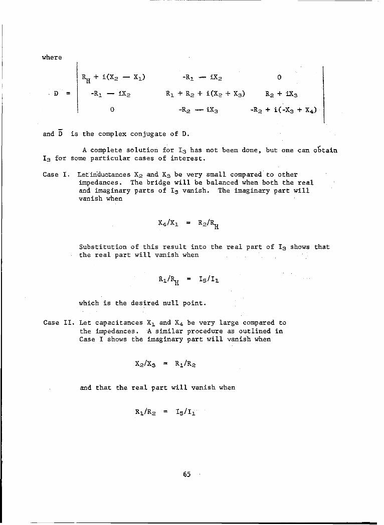
where
RH+ i(X 2 - XI) -I- iX2 0
D -R= X R, +R 2 +i(X 2 +X 3 ) R 2 +iX 3
0 -2- iX3 -R2 + i(-X 3 + W4
and Di is the complex conjugate of.D.
A complete solution for 13 has not been done, but one can o5 tain13 for some particular cases of interest.
Case I. Letin~ductances X2 and X3 be very small compared to otherimpedances. The bridge will be balanced when both the realand imaginary parts of 13 vanish. The imaginary part willvanish when
x41/x1 = R/
Substitution of this result into the real part of 13 shows thatthe real part will vanish when
R/H= 15/11
which is the desired null point.
Case II. Let capacitances X, and X4 be very large compared tothe impedances. A similar procedure as outlined inCase I shows the imaginary part will vanish when
X/3= RI/R2
and that the real part will vanish when
R1/R2 = 15/11
65
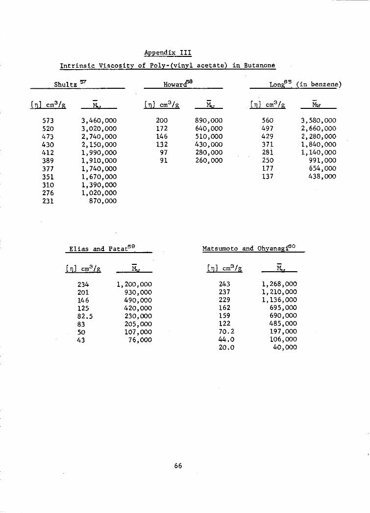
Appendix III
Intrinsic Viscosity of Poly-(vinyl acetate) in Butanone
Shultz 57 Howarcp Long 5 (in benzene)
[E] cm3 /g I En] cm 3 /g I En] cm3 /g
573 3,460,000 200 890,000 560 3,580,000520 3,020,000 172 640,000 497 2,660,000473 2,740,000 146 510,000 429 2,280,000430 2,150,000 132 430,000 371 1,840,000412 1,990,000 97 280,000 281 1,140,000389 1,910,000 91 260,000 250 991,000377 1,740,000 177 654,000351 1,670,000 137 438,000310 1,390,000276 1,020,000231 870,000
Elias and Patat5 9 Matsumoto and Ohyanagi 6 0
En] cm3 /g % En] cm3 /g T.,
234 1,200,000 243 1,268,000201 930,000 237 1,210,000146 490,000 229 1,136,000125 420,000 162 695,00082.5 230,000 159 690,00083 205,000 122 485,00050 107,000 70.2 197,00043 76,000 44.0 106,000
20.0 40,000
66

BIBLIOGRAPHY
1. P. Debye, J. Appl. Phys. 51, 18 (1947).
2. B. H. Zinm, R. S. Stein, and P. Doty, Polymer Bull. 1, (1945).
3. M. Fixman, J. Chem. Phys. 23, 2074 (1955).
4. B. H. Zimm, J. Chem. Phys. 16, 1093 (1948).
5. W. G. McMillan and J. E. Mayer, J. Chem. Phys. 13, 276 (1945).
6. A. C. Albrecht, J. Chem. Phys. 27, 1014 (1957).
7. P. J. Flory, J. Chem. Phys. 17, 1347 (1949).
8. P. J. Flory and W. R. Krigbaum, J. Chem. Phys. 18, 1086 (1950).
9. P. J. Flory and A. M. Bueche, J. Polymer Sci. 27, 219 (1957).
10. E. F. Casassa, J. Chem. Phys. 27, 970 (1957).
11. E. F. Casassa and H. Markovitz, J. Chem. Phys. 29, 493 (1958).
12. E. F. Casassa, J. Chem. Phys. 31, 800 (1959).
13. See for example, J. 0. Hirschfelder, C. F. Cutiss, and R. B. Bird,Molecular Theor of Gases and Liquids (John Wiley & Sons, Inc.,New York, 1957) p. 891'ff.
14. B. H. Zimm, J. Chem. Phys. 14, 164 (1946).
15. M. Fixman, J. Chem. Phys. 23, 1656 (1955).
16. H. C. Brinkman and J. J. Hermans, J. Chem. Phys. 17, 574 (1949).
17. W. H. Stockmayer, J. Chem. Phys. 18, 58 (1950).
18. J. G. Kirkwood and R. J. Goldberg, J. Chem. Phys. 18, 54 (1950).
19. J. J. Blum and M. F. Morales, J. Chem. Phys. 20, 1822 (1952).
20. See H. E. Stanley, Thesis, Massachusetts Institute of Technology (1949).
21. E. F. Casassa and I. H. Billick, J. Am. Chem. Soc. 78, 1377 (1957).
67

22. Tables of the Error Function and Its Derivatives (U. S. GovernmentPrinting Office, Washington, D. C., 1954).
23. H. M. Terrill and L. Sweeny, J. Franklin Inst. 237, 495 (1944);238, 220 (1944).
24. J. J. Hermans, Rec. Trav. chim. 68, 859 (1949).
25. H. Benoit and M. Goldstein, J. Chem. Phys. 21, 947 (1953).
26. H. G. Dawson, Proc. London Mathematical Soc. 29, 521 (1898).
27. B. Lohmander and S. Rittsten, K. Fysiogr. Salsk. Lund. Forhandl,28, 45 (1958).
28. P. J. Flory and T. G Fox, Jr., J. AmxwChem. 'Soc. 7Z3 1904 (1951).
29. P. J. Flory, J. Chem. Phys. 17, 1347 (1949); P. J. Flory andW. R. Krigbaum, ibid. 18, 1086 (1950).
30. T. A. Orofino and P. J. Flory, J. Chem. Phys. 26, 1067 (1957).
31. P. J. Flory, Principles of Polymer Chemistry, Cornell UniversityPress, Ithaca, New York (1953), Chapter XIV.
32. T. G Fox, to be published.
33. T. G Fox, Jr., and P. J. Flory, J. Am= Chem. Soc. 73.1909 (1951).
34. P. J. Flory, 0. K. Spurr, Jr., and D. K. Carpenter, J. PolymerSci. 27, 231 (1958).
35. W. R. Krigbaum and P. J. Flory, J. Am. Chem. Soc. 7_6 3758(1954).
36. T. G Fox and P. J. Flory, J. Phys. and Colloid Chem. 53,197 (1949).
37. T. Kawai and R. Naito, J. Applied Polymer Sci. 3, 232 (1960).
38. C. Rossi, V. Bianchi and E. Bianchi, Makromol. Chem. 4131 (1960).
39. P. J. Flory and T. G Fox, J. Am. Chem. Soc. 73, 1904 (19.51);ibid. 1909 1915.
68

40. P. J. Flory, J. Chem. Phys. 17, 303 (1949).
41. P. J. Flory, Principles of Polymer Chemistry, Cornell UniversityPress, Ithaca, New York (1953).
42. T. A. Orofino and P. J. Flory, J. Chem. Phys. 26, 1067 (1957).
43. P. J. Flory, 0. K. Spurr, Jr., and D. K. Carpenter, J. PolymerSci. 27, 231 (1958).
44. P. Outer, C. I. Carr and B. H. Zimm, J. Chem. Phys. 18830 (1950).
45. T. G. Fox, et al. to be published.
46. T. G Fox, et al. to be published.
47. W. R. Krigbaum and P. J. Flory, J. Polymer Sci. 11, 37 (1953).
48. D. C. Pepper, Sci. Proc. Roy. Dublin Soc., 25, 239 (1951).
49. D. McIntyre and M. C. Doderer, J. Res. Nat. Bur. Std., 62153 (1959).
50. S. Katz, private communication.
52. H. Sheffer and J. Hyde, Can. J. Chem. 30, 817 (1952).
53. E. F. Casassa and S. Katz, J.PolymerSci. 14, 385 (1954).
54. L. Kushner, J. Opt. Soc. Am. 44, 155 (1954).
55. J. J. Hermans and S. Levinson, J. Opt. Soc. Am. 41, 460(1951).
56. R. Engstrom, J. Opt. Soc. Am. 37, 420 (1947).
57. A. R. Shultz, J. Am. Chem. Soc. 76, 3422 (1954).
58. R. 0. Howard, Ph.D. Thesis, Massachusetts Institute of TechnologyCambridge, Massachusetts, 1952.
69

59. H. G. Elias and F. Patat, Makromol. Chem. 25, 13 (1958).
60. M. Matsumoto and Y. Ohyanagi, J. Polymer Sci. 46, 441 (1960).
61. Technical Report No. 3, Office of Naval Research, Contract Nonr-3693(00),February 29, 1960.
62. C. I. Carr, Jr., and B. H. Zimm, J. Chem. Phys. 18• 1616 (1950).
63. B. H. Zimm, J. Phys. and Colloid Chem. 5. 260 (1948);J. Chem. Phys. j6, 1093, 1099 (1948).
64. M. L. Huggins, J. Am. Chem. Soc., 64, 2716 (1942).
65. V. C. Long, Ph.D. Thesis, University of Michigan, Ann Arbor, Michigan,1958.
70
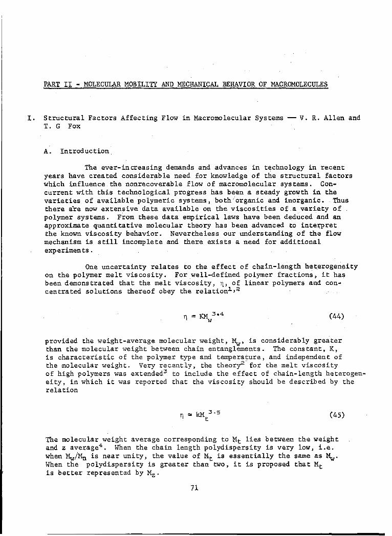
PART II - MOLECULAR MOBILITY AND MECHANICAL BEHAVIOR OF MACROMOLECULES
I. Structural Factors Affecting Flow in Macromolecular Systems -- V. R. Allen andT. G Fox
A. Introduction
The ever-increasing demands and advances in technology in recentyears have created considerable need for knowledge of the structural factorswhich influence the nonrecoverable flow of macromolecular systems. Con-current with this technological progress has been a steady growth in thevarieties of available polymeric systems, both'organic and inorganic. Thusthere are now extensive data available on the viscosities of a variety ofpolymer systems. From these data empirical laws have been deduced and anapproximate quantitative molecular theory has been advanced to interpretthe known viscosity behavior. Nevertheless our understanding of the flowmechanism is still incomplete and there exists a need for additionalexperiments.
One uncertainty relates to the effect of chain-length heterogeneityon the polymer melt viscosity. For well-defined polymer fractions, it hasbeen demonstrated that the melt viscosity, I, of linear polymers and con-centrated solutions thereof obey the relation1 ,'2
= -w 3 4 (44)
provided the weight-average molecular weight, M., is considerably greaterthan the molecular weight between chain entanglements. The constant, K,is characteristic of the polymer type and temperature, and independent ofthe molecular weight. Very recently, the theory# for the melt viscosityof high polymers was extended3 to include the effect of chain-length heterogen-eity, in which it was reported that the viscosity should be described by therelation
T = kM t3"5 (45)
The molecular weight average corresponding to Mt lies between the weightand z average . When the chain length polydispersity is very low, i.e.when Mw/Mn is near unity, the value of Mt is essentially the same as Mw.When the polydispersity is greater than two, it is proposed that Mtis better represented by Mz.
71
In apparent contradiction to the theory, it has been reportedthat the viscosities of whole polymers of known distributions,6 and ofmixtures of polymer fractions7 are adequately expressed by Eq. (44). Con-sequently, it would seem that a need is indicated for additional informationrelating polymer melt viscosity to chain length in the high molecular weight
region with particular emphasis on both the degree of polydispersity and the
nature of the distribution.
There exists even greater uncertainty concerning the [i]-Mrelation for the low molecular weight region both because of the relativescarcity of data and because of the increased complexity of the relationship.
The log-log plots of viscosity versus chain length for various polymers areseldom linear over a broad range of chain length in this low molecularweight region. Further, for these samples of lower average chain length,
both the slope and/or shape of the relation seem to be temperature-dependent. Although according to theory2 , the polymer viscosity should
be proportional to the first-power of the chain length in this region, it
has been recognized8 ,9 that variation with molecular weight of local factorsbecome increasingly important with decreasing chain length. This influence
of the change in the "free volume" of the polymer with chain length, as
expressed by the change in Tg, is also demonstrated by the isothermal
viscosity-molecular weight concentration of diluent relationships' 0 .
Even fewer data are available concerning the effect of chainlength heterogeneity in this low molecular weight region. Furthermore,
the theory of Bueche 3 does not apply to polydispersity for low molecular-weight polymers. Consequently, a definite need is indicated for additionaldata in this low molecular weight region in order to allow a better under-
standing of the factors which affect the viscous flow of short-chain
polymers.
This report constitutes a preliminary description of proceduresand results in the general investigation of structural factors affecting
flow in macromolecular systems. The objectives are to extend the present
knowledge of:
(i) the effect of chain length heterogeneity on viscous flowin both the high and low molecular weight regions.
(2) the effect of diluents on the 1 -M relation, and
(3) the possible effect of chain stereoregularity on both
the viscosity and concentration and chain entanglements.
Because of the availability of polystyrene samples having avery low polydispersity, prepared by anionic polymerization methods, and,because of the large amount of data on fractions of this polymer in the
literature, it has been decided to use it for the bulk of this investigation.
72
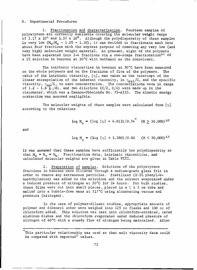
B. Experimental Procedures
1. Fractionation and characterization. Fourteen samples ofpolystyrene are currently available covering the molecular weight rangeof 1.17 x 10⁴ and 1.37 x 10⁶. Although the polydispersity of these samplesis very low (Mw/Mn - 1.05 - 1.10), it was decided to fractionate each intoabout four fractions with the express purpose of removing any very low (andvery high) molecular weight material. At present, eight of the polymershave been separated into 3-4 fractions via a one-stage fractionation1 i of
a 1% solution in benzene at 30'C with methanol as the nonsolvent.
The intrinsic viscosities in benzene at 30'0 have been measuredon the whole polymers and on the fractions of five of the polymers. Thevalue of the intrinsic viscosity, [rI], was taken as the intercept of thelinear extrapolation of the inherent viscosity, ln Trel/C, and the specificviscosity, sp/c, to zero concentration. The concentrations were in range
of 1.2 - 1.6 g./dl. and two dilutions (C/2, C/4) were made up in theviscometer, which was a Cannon-Ubbelohde No. 75-A133. The kinetic energycorrection was assumed negligible.
The molecular weights of these samples were calculated from [I]according to the relations
log Mv - (log [T] + 4.013)/0.74* (M > 30,000)12
and
log Mv = (log [i] + 3.380)/0.60 (H < 30,000)13
It was assumed that these samples have sufficiently low polydispersity sothat Mn = Mv = Mw. Fractionation data, intrinsic viscosities, andcalculated molecular weights are given in Table VIII.
2. Preparation of samples. Solutions of the polystyrenefractions in benzene were filtered through a medium-grade glass frit inorder to remove any extraneous particles. Stabilizer (0.5% phenyl-b-naphthylamine) was added to the solutions and the solvent evaporated undera reduced pressure of nitrogen at 50'C for 24 hours. For bulk studies,these films were cut into small pieces, placed in a 1 x 5 cm tube andmelted into a bubble-free mass at 2170C using alternating vacuum andpressure (nitrogen).
In the case of polymer-diluent studies, appropriate amounts ofpolymer. and dibenzyl ether were weighed into 125 cc flasks and 100 cc ofchloroform added. This solution was cast into chloroform-extrated, taredaluminum dishes and the chloroform evaporated under reduced pressure ofnitrogen of 40 0 C with a steady flow of nitrogen being maintained. After
This particular relationship was used so that melt viscosity data couldbe compared with reported7 values.
73
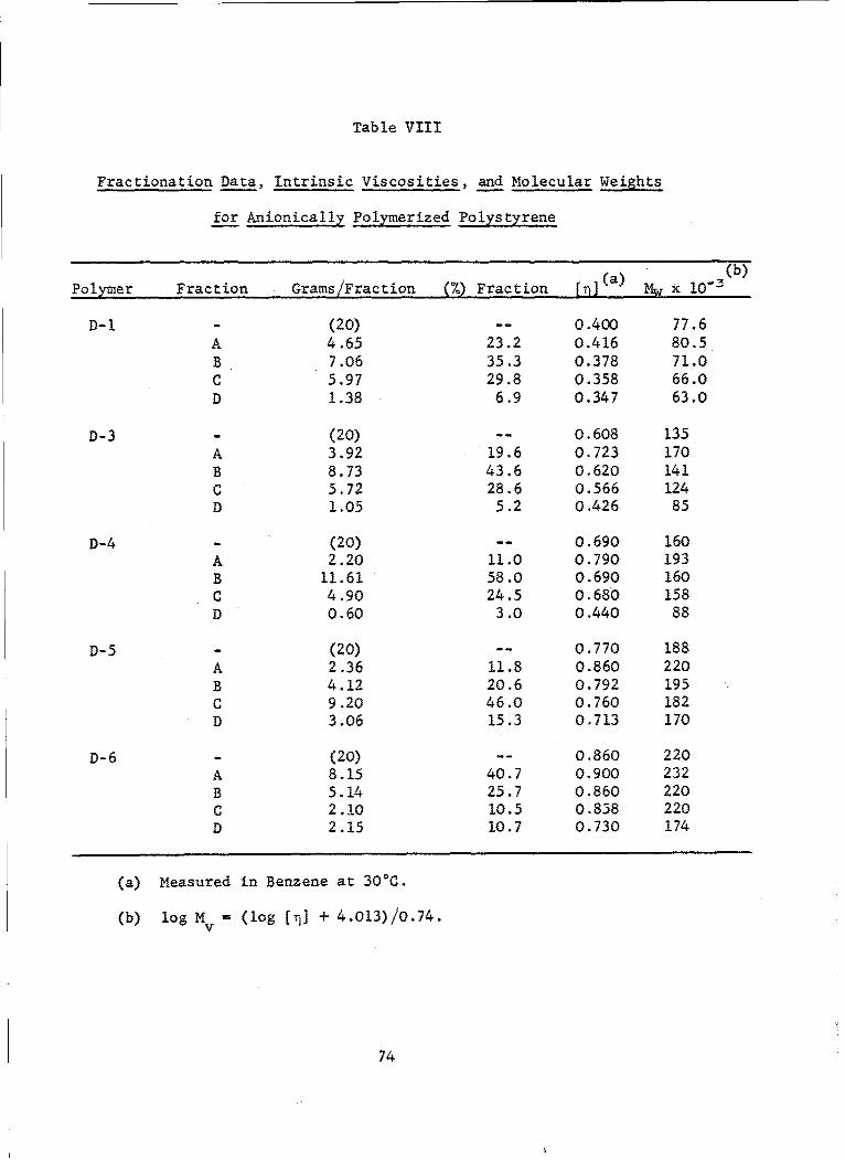
Table VIII
Fractionation Data, Intrinsic Viscosities, and Molecular Weights
for Anionically Polymerized Polystyrene
Polymer Fraction Grams/Fraction (%) Fraction [rJ] (a) N X 10"3
D-l - (20) -- 0.400 77.6A 4.65 23.2 0.416 80.5B 7.06 35.3 0.378 71.0C 5.97 29.8 0.358 66.0D 1.38 6.9 0.347 63.0
D-3 - (20) -- 0.608 135A 3.92 19.6 0.723 170B 8.73 43.6 0.620 141C 5.72 28.6 0.566 124D 1.05 5.2 0.426 85
D-4 - (20) -- 0.690 160
A 2.20 11.0 0.790 193B 11.61 58.0 0.690 160
c 4.90 24.5 0.680 158D 0.60 3.0 0.440 88
D-5 - (20) -- 0.770 188A 2.36 11.8 0.860 220B 4.12 20.6 0.792 195C 9.20 46.0 0.760 182D 3.o6 15.3 0.713 170
D-6 - (20) -- 0.860 220A 8.15 40.7 0.900 232B 5.14 25.7 0.860 220o 2.10 10.5 0.838 220D 2.15 10.7 0.730 174
(a) Measured in Benzene at 300C.
(b) log m = (log ([I] + 4.013)/0.74.
74

three days, the decrease in rate of the polymer-diluent mixture (0.05% byweight of the diluent per 24 hours) indicated that the chloroform had beenremoved. [Analytical tests are in progress to determine the exact con-centration of ingredients after this drying procedure. Unless thesetests indicate otherwise, the above procedure will be followed in preparingthe polymer-diluent mixtures.] These concentrated polymer solutions willthen be transferred to the 1 x 5 cm tubes and treated as above.
3. Melt viscosity. For the measurement of melt viscosity, anapparatus was constructed which is a model of that described by Fox, Gratch,and Loshaek' 4 . A scale model is diagrammed in Fig. 17. Temperature controland flexibilitywere achieved through the use of different vapor baths con-taining diethylene glycol (244.50C), naphthalene (2170C), cyclohexanol(161.50C), and toluene (110.80C). (A thermostated oil bath will be usedif lower temperatures should be required.)
Eight different sizes of viscometers (thirty-three in all) areavailable of the capillary type, i.e. straight, uniform-bore. The lengthof the capillary portion varies from 7.0 to 20 cm with 43 to 30 cm of 8 mmtubing fused to the capillary. There are four successive marks along thecapillary with the first mark being one cm from the tip. This arrangementallows three viscosity determinations to be made with a single capillary.
Four viscometers are of the capillary pipette type, having abulb ca. 12 mm in diameter located at various distances (7.0, 16.0, and25 cm) from the tip. The reference marks are located on the uniform-boreportions immediately adjacent to the bulb. Thus, only a single viscositydetermination is obtained per capillary.
The viscometers were calibrated by H. Nakayasu, formerly of thislaboratory, against selected National Bureau of Standards oils and fromthe bore dimensions1 4 . A recalibration and reproducibility check wasmade on twelve viscometers (three different sizes) using Oronite polybutene128 (TI = 5400 poises at 25.05 + 0.050C). An example of the reproducibilityachieved in these measurements is demonstrated by the results obtained ontwo similar viscometers having calibration constants, as measured byNakayasu, of ca. 1000 poises/cm.Hg/min. With an applied nitrogen pressureof 3.5-4.0 cm Hg and flow times of 1.0-1.6 minutes, the result of twelvemeasurements was I = 5392 poises with a maximum deviation of + 2.2%. Thisnot only indicates the reproducibility expected in these measurements butalso points out the excellent reliability of the constants determined byNakayasu, which are listed in Table IX for each type of viscometer.
There were slight discrepancies noted in four of the viscometerswhich were checked. For example, the viscosities measured between marks1-2 and 3-4 of a certain viscometer were in agreement with the value forthe polybutene, but the viscosities measured between marks 2-3 were con-sistently higher by 4%, using the constants determined by Nakayasu.Until such time as these viscometers can be checked against severalstandard oils, they will not be used.
75
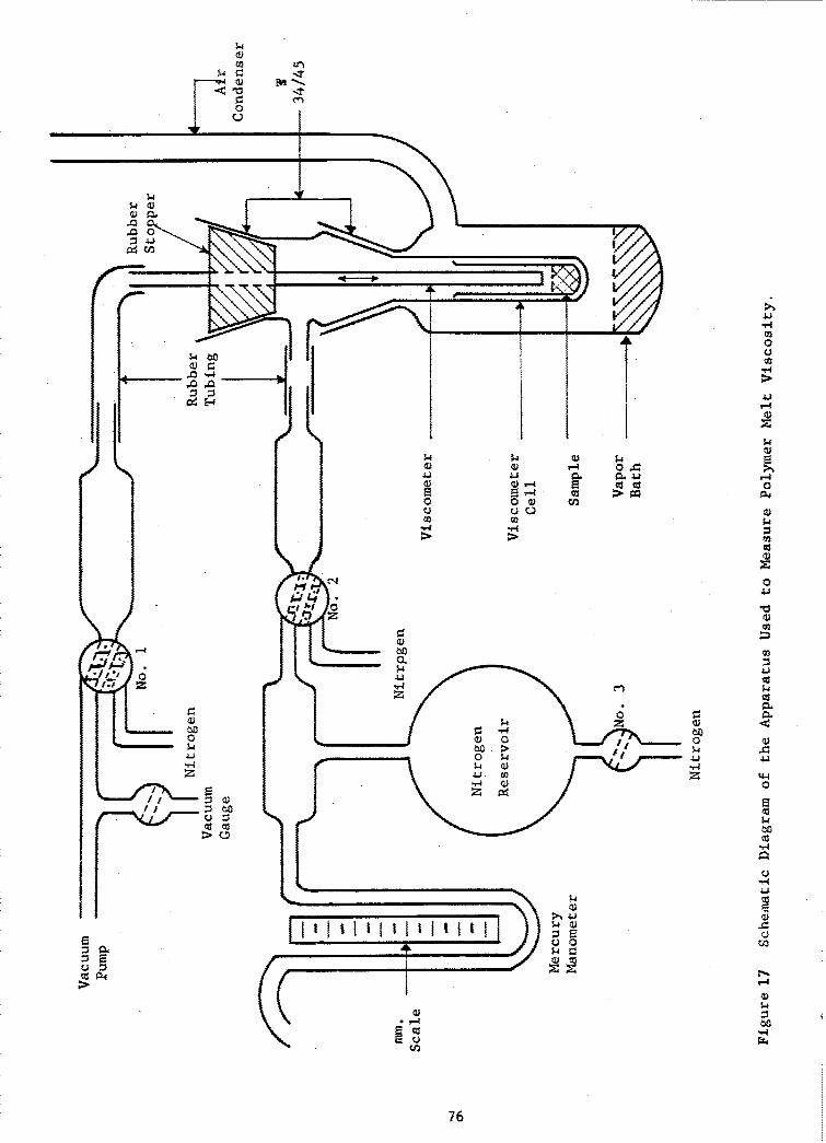
,4
0
,a 0
0
4Z -,
0 (10
V44>0
414C- 0r o
U Oto4
0 4J
z ;44
10
-,4-41
tv 54
(UU14 to
Cs .10
76

Tab le IX
Viscometer Dimensions and Calibration Cons tants(I)
Capillary Capillary(2) Capillary Constants (poise/minmcm Hg)
Bore (mm) Length (cm) A(3) B(3) C(3)
Pipette Type
0.5 5 0.013780.5 10 0.017661.0 15 0.16901.0 7.5 0.3825
Straight Capillary Type
0.5 20.5 1.005 1.002 0.9900.5 15.0 1.989 2.081 1.9621.0 19.0 4.575 5.331 4.8851.0 13.5 9.981 9.917 9.4841.0 9.5 24.515 25.424 24.7123.o 14.5 97.515 98.939 93.2513.o 7.0 498.84 435.27 472.473.o 7.0 1052.6 1115.5 1033.4
(1) Determined by H. Nakayasu of this laboratory.
(2) Overall length of the uniform-bore capillary.
(3) Corresponding to the flow lengths between successive marks.
A brief description is given for the general procedure used inthe measurement of the melt viscosity with occasional reference to Fig. 17.
The sample (ca. 2-3 grams) is placed in a 1 x 5 cm pyrextube which is in turn placed in the sample holder. Theappropriate viscometer is positioned just above the surfaceof the sample and the air replaced by nitrogen by successiveaddition of nitrogen and evacuation. Heat is then appliedto the vapor bath and the sample is heated as far above itssoftening point as possible, without causing degradation.Stopcock #1 is then rotated until no more gas bubblesappear and a clear melt is obtained. This removes volatileimpurities. The sample is now ready for the viscositymeasurement.
77
The flow of nitrogen through Stopcock #1 isstopped and the lower end of the capillary is insertedinto the clear melt. After a predetermined time toallow the system to reach thermal equilibrium, nitrogenpressure (2-25 cm Hg as required to give a reasonableflow time 2-3 minutes) is applied by opening Stopcock#2 which connects the pressure reservoir (ca. one liter)to the viscometer assembly. This forces the polymerup the capillary.
The flow time between successive marks is measuredand the average pressure is read from the mercurymanometer. This is corrected for mean difference inheight between the polymer in the capillary and thesurface of the melt. After the polymer reaches thefourth mark (or earlier), Stopcock #2 is closed and#3 is opened, releasing the pressure. A reversepressure of nitrogen is applied through Stopcock #1,causing the polymer to flow slowly out of the viscometer.
The melt viscosity of the polymer is then calculated from themeasured flow time and applied pressure (corrected) and from thecapillary constant.
C. Results and Discussion
It is necessary that the polymer samples have a sufficientlylow degree of polydispersity to allow reliable interpretation of theviscosity data. Therefore, it is also important that the characterizedfractions do not undergo any changes prior to measurement of the viscositywhich would affect the chain-length distribution. A thermal stabilitystudy was initiated to insure that this type polystyrene, prepared byanionic polymerization methods, could withstand the extreme temperaturesto which it would eventually be subjected.
In the molecular weight range of 6-8 x 10⁴, heating for one-two hours at 217'C is necessary to cause a two-gram sample to flow into abubble-free mass suitable for capillary-viscosity measurements. For asample having a molecular weight of 2 x 10⁵, the required heating timeincreases to four-five hours. Some preliminary viscosity measurements onwhole polymers indicated that the thermal stability of this type ofpolymer is relatively poor, a 15-20% decrease in ri being observed in onehour at 217' under an atmosphere of nitrogen. Consequently, a comparativestudy was made of the effect on both the melt viscosity, ri, and theintrinsic viscosity, [T1], of heating at 217°C under conditions correspondingto those during the measurement of the melt viscosity. The results, listedin Table X and shown in Fig. 18, clearly demonstrate that the stabilizeris required to prevent degradation during the lengthy heating period,leading to an increase in chain-length polydispersity.
78
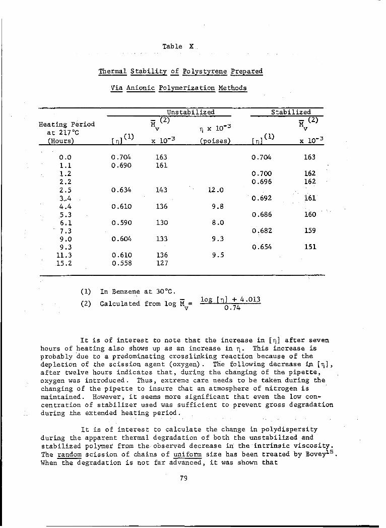
Table X,
Thermal Stability of Polystyrene Prepared
Via Anionic Polymerization Methods
Unstabilized Stabilized
Heating Period (2) R (2)
at 2170C v q x 10-) v
(Hours) [I] () x 10-: (poises) [1nI) x 10"3
0.0 0.704 163 0.704 1631.1 0.690 1611.2 0.700 1622.2 0.696 1622.5 0.634 143 12.03_4 0.692 1614.4 0.610 136 9.85.3 0.686 1606.1 0.590 130 8.07.3 0.682 1599.0 0.604 133 9.39.3 0.654 15111.3 0.610 136 9.515.2 0.558 127
(1) In Benzene at 300C.
(2) Calculated from log M = log [fl] + 4.013v 0.74
It is of interest to note that the increase in [TI] after sevenhours of heating also shows up as an increase in TL. This increase isprobably due to a predominating crosslinking reaction because of thedepletion of the scission agent (oxygen). The following decrease ini [I],after twelve hours indicates that, during the changing of the pipette,oxygen was introduced. Thus, extreme care needs to be taken during thechanging of the pipette to insure that an atmosphere of nitrogen ismaintained. However, it seems more significant that even the low con-centration of stabilizer used was sufficient to prevent gross degradationduring the extended heating period.
It is of interest to calculate the change in polydispersityduring the apparent thermal degradation of both the unstabilized andstabilized polymer from the observed decrease in the intrinsic viscosity.The random scission of chains of uniform size has been treated by Bovey' 5 .When the degradation is not far advanced, it was shown that
T9
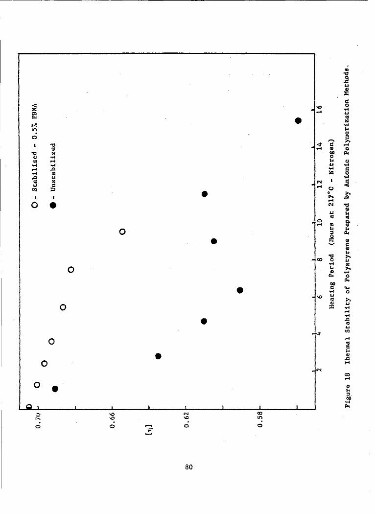
0
z '-4
414
I El
I ~ i-4 El0
0 N4 0
A A4
El 0l
oto44
0 0
800

Pw/P = (2/S 2 )(e +S-l) (46)
where Pw and Po are the degree of polymerization of the degraded sampleand the original sample, respectively, and S is the number of scissionsper primary chain. Also, regardless of how far the degradation hasproceeded, it was shown that
P = I/(l+S) (47)
where Pn is number-average degree of polymerization of the degraded sample.
The number of chain scissions per primary chain was calculatedusing (3) and the molecular weights given in Table X. For this it wasassumed that Mv Z M
v wThen the number-average degree of polymerization was calculated
from (4) and the polydispersity M /M was determined. The results of thesecalculations are presented in TabYe nXI. It is apparent from these valuesthat stabilizer is necessary, particularly for the high molecular weightsamples which require extended treatment at high temperatures in order toobtain a clear melt suitable for viscosity measurements. Further, it isclear from these calculations that every effort should be made to reducethe required heating period and to insure the exclusion of air from thesample during successive measurements.
Table XI
Polydispersity of Degraded Polystyrene(a)
Polymer Stabilized(b) Unstabilized
Heating Period (Hours at 2170C) 5.0 6.1
"M (original) 160,000 160,000v
"M (degraded) 150,000 120,000v
Scissions per chain 0.2 0.95
Mw/Mn 1.12 1.46
(a) Calculations based on treatment of Bovey' 5 .
(b) 0.5% phenyl-b-naphthylamine.
81
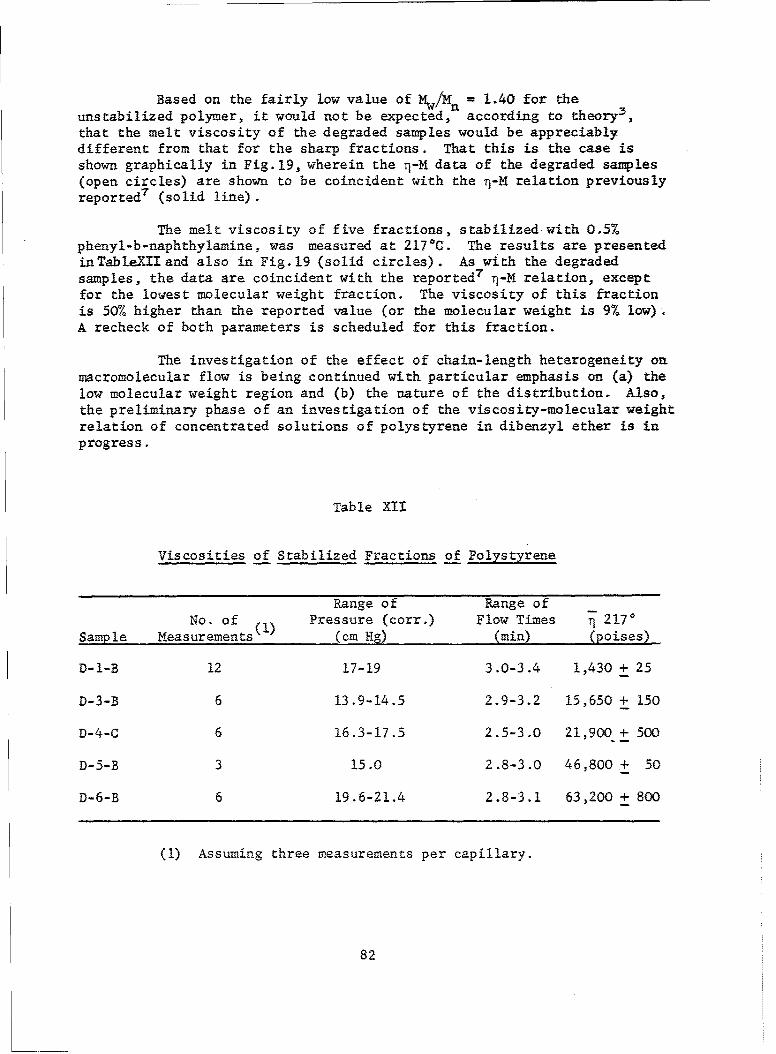
Based on the fairly low value of Mw/Mn = 1.40 for theunstabilized polymer, it would not be expected, according to theory,that the melt viscosity of the degraded samples would be appreciablydifferent from that for the sharp fractions. That this is the case isshown graphically in Fig.19, wherein the r1-M data of the degraded samples(open circles) are shown to be coincident with the I-M relation previouslyreported7 (solid line).
The melt viscosity of five fractions, stabilized with 0.5%phenyl-b-naphthylamine, was measured at 217°C. The results are presentedinTableXII and also in Fig. 19 (solid circles). As with the degradedsamples, the data are coincident with the reported7 q-M relation, exceptfor the lowest molecular weight fraction. The viscosity of this fractionis 50% higher than the reported value (or the molecular weight is 9% low).A recheck of both parameters is scheduled for this fraction.
The investigation of the effect of chain-length heterogeneity onmacromolecular flow is being continued with particular emphasis on (a) thelow molecular weight region and (b) the nature of the distribution. Also,the preliminary phase of an investigation of the viscosity-molecular weightrelation of concentrated solutions of polystyrene in dibenzyl ether is inprogress.
Table X1I
Viscosities of Stabilized Fractions of Polystyrene
Range of Range ofNo. of Pressure (corr.) Flow Times rj 2170
Sample Measurements (cm Hg) (min) (poises)
D-I-B 12 17-19 3.0-3.4 1,430 + 25
D-3-B 6 13.9-14.5 2.9-3.2 15,650 + 150
D-4-C 6 16.3-17.5 2.5-3.0 21,900 + 500
D-5-B 3 15.0 2.8-3.0 46,800 + 50
D-6-B 6 19.6-21.4 2.8-3.1 63,200 + 800
(1) Assuming three measurements per capillary.
82
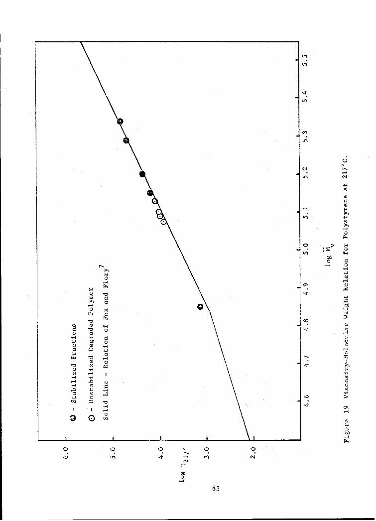
0
C,
-41
U,4
02
4-440a
-4
N4 -4-4
r-4 0
-2 .144~4-1 > -j
'0 0
I -44-4 .- gr0
'-4 ,a to
.83

II. An attempted Stereospecific Emulsion Polymerization of Vinyl AcetateEmploying Protein-Detergent Solubilizing Agents - V. R. Allen andT. G. Fox
A. Introduction
Breuer and Strauss, in an unpublished manuscript' 6 , havesuggested recently the use of protein-detergent complexes in free-radicalemulsion polymerizations to obtain stereoregular polymers. Because ofthe conveniences associated with polymerization in emulsion, it was con-sidered of interest to prepare a vinyl polymer having a stereoregularstructure employing this new technique. Such a polymer would be valuablein the study of the factors affecting flow in macromolecular systems.
We report here the results of this investigation of the appli-cation of the Breuer-Strauss technique to the polymerization of an emul-sion of vinyl acetate stabilized by a bovine serum albumin-sodium dodecylsulfate complex. A brief description is given of the experimentalmethods followed by the description of results to date. Although thepreliminary present evidence suggests that crystalline products are ob-tained in some instances, the reproducibility is very poor. Hence, theresults of this preliminary study, though quite striking, are not con-clus ive.*44*
B. Experimental Methods
i. Polymerization conditions. The polymers were prepared inan emulsion system according to the method reported by Breuer and Straussis.The polymerization recipe, as given in Table XIIIwas used, except as notedelsewhere.
Note added in proof (11-15-61): Originally in this manuscript we re-corded observations on diffraction patterns and unique physical andchemical properties which suggested the presence of a crystalline componentin six of the thirty-eight polymerization products. Subsequently, (cf.Quarterly Report 17, Nov. 15, 1961) we found that these samples were con-taminated with sodium calcium silico aluminate introduced as an impurityin the sodium chloride used to coagulate the polymer in the early experi-ments; in addition, there were evidences of the presence of detergent ina crystalline form in a few samples. Since the original observationssuggesting crystallinity were shown to be of no significance in this study,they have been deleted from this report.
84

Table XIII
Emulsion Recipe for Vinyl Acetate
Water (0 2 -free) 100
Vinyl Acetate (dist.) 100
Bovine Serum Albumin (BSA)' 3.5
Sodium Dodecyl Sulfate (SDS) 2 1.6
Potassium Persulfate 3 0.3
1. Nutritional Biochemicals Company - Crystalline Grade.2. Fisher Scientific Company - Reagent Grade.3. Eastman Company - Reagent Grade.
A typical polymerization may be described as follows:
3.5 g. of albumin was dissolved in 100 ml of 02 -freewater under nitrogen. The detergent and initiator werethen added and allowed to dissolve. After solution, nitro-gen was bubbled in for five minutes and the solution chilledin a refrigerator.
100 g. of freshly-distilled vinyl acetate (chilled)was added through a self-sealing rubber stopper with alarge syringe. The system was then flushed with nitrogenfor five minutes and placed in the thermostatically con-trolled water bath.
After a considerable induction period of one to thirtyhours, the flask was removed from the bath after a giventime and the latex poured (or spooned) into ca. threeliters of concentrated NaCl solution. The polymer wasfiltered, washed with water, and dried in vacuo at 50 0 C.The conversion was calculated from the weight of driedpolymer.
2. Coagulation and solubility. Although mentioned in thetypical experiment above, the method of coagulation of the polymer isdescribed more fully. In the earliest runs, it was found that sufficientNaCl remained in the polymer after the washing to produce faint lines inthe x-ray diffraction pattern. Consequently, in some of the later runs,the polymer was removed from the salt solution by filtration and redis-persed in distilled water. After soaking 24 hours in successive portionsof water, residual salt could not be detected by x-ray. The alternativemethod of coagulating in distilled water was also used although the soapmade filtration difficult.
85

The solubility of the dried polymer was measured qualitativelyby placing a small piece (0.1 g) in 2-3 ml of the desired solvent. Thequantitative measurement of solubility (which is referred to in the de-scription of results) was obtained by placing one-gram samples of thepolymer in 100 ml of acetone with stirring. After 24 hours, the residuewas allowed to settle (or centrifuged) and the solution decanted off.This procedure was repeated three times. The solubility was calculatedfrom the weight of dried, soluble polymer.
3. Hydrolysis and reacetylation. The polymers to be hydro-lyzed were in the form of thin strips cut from either cast or pressedfilms. The hydrolysis was carried out in small flasks, equipped withcondensers, on a steam plate. Fifty milliliters (excess) of either 4MNaOH or 6M HCI were added to one gram of polymer and heated for 24 to 48hours. The mixture was dialyzed against distilled water until neutral.
Reacetylation of these hydrolysates was according to themethod of Melville and Sewell 1 7 . After 48 to 96 hours on the steam plate,the excess acid was neutralized with IM NaOH and the product dialyzed.
4. Infrared spectra. The IR spectra of the various polymerswere obtained using a Perkin-Elmer "Infracord". The samples were eitherin the form of cast films, pressed films, or KBr pellets.
C. Results
Poly-(vinyl acetate) PVAc, prepared in emulsion according tothe recipe given in TableXIlIwithout the BSA, hereinafter referred to asconventional polymer, is soluble in ketones, lower alcohols, and aro-matics. It flows readily at slightly elevated temperatures (Tg - 35 0 C)and is rapidly (-2 hours) hydrolyzed by dilute acid or base at 100°C intoa water-soluble product which can be easily crystallized. This poly-(vinyl alcohol) PVA can be reacetylated; the product having propertiesessentially identical to the original PVAc.
The x-ray diffraction pattern of this PVAc is tygical of anamorphous polymer, having a strong absorption band at 7.0 A and a slightlyweaker band at 4.0 A. Regardless of prior sample treatment, annealing,stretching, etc., this pattern persists.
The inclusion of the BSA in the emulsion recipe results in aproduct containing an insoluble phase (in acetone), even at low conver-sions, which contains tightly bound protein in quantities up to 20% byweight, as measured by nitrogen (Kjeldahl) analysis. The soluble phase,in every case, contains no protein. Numerous tests on the propertieslisted above for this soluble phase show that it is indistinguishable fromthe conventional polymer. Consequently, this phase need not be mentionedfurther, except occasionally for comparative purposes.
86

There is presented in Table XIV the experimental conditionsfor thirteen of the thirty-eight polymerizations which were attempted.Of the remaining, fourteen may be considered duplicates of one or moreof those listed, three were lost by frothing of the latex due to ex-cessive heat build-up, and eight, which were modifications of the basicsystem(Table XIII),either failed to polymerize or yielded the conventionalproduct.
1. Solubility and protein content. The solubility is one ofthe more interesting properties of the polymers of vinyl acetate preparedaccording to the Breuer-Strauss technique. There is presented inTable XIV the results of solubility measurements of these polymers incold (30') acetone, normally a good solvent for PVAc.
Table XIV
Polymerization Conditions and Polymer Properties
Induction Polymerization2 Con- Insolubility BoundTemp. Period Period version in Acetone Protein
Polymer (°C) (Hours) (Hours) (%) (%) M%)
VC-i 30 9 9 88 0 0
VC-2 28 1 2 30 0 0
VT-I 30 9 9 80 100 3
VT-16 20 20 0.5 1.6 100 20.4
VT-20 35 2 2 19.3 90 13.7
VT-21 33 5 3 18.0 70 6.0
VT-23 33 21 3 30.0 50 11.1
VT-28 30 5 3 18.2 56 16.2
VT-29 30 5 3 18.3 65 19.7
VT-22 40 2 2 27 96 5.0
VT-15 28 1 3 35 52 7.4
VT-19 25 27 5 72 32 5.0
VT-II 30 8 4 30 0 0
1 Time to appearance of blue fluorescense.
2 Time after blue fluorescence.
87

The gels were swollen slightly and films could be formed on evaporationof the solvent. Examination of these films in a polarizing microscoperevealed that considerable strain was present. When the strained portionswere heated to 70-80', these strain patterns disappeared but appearedagain as the sample cooled to room temperature. These acetone-extractedgels were resistant to other types of solvents, e.g. ethers, alcohols,esters, and substituted benzenes, at various temperatures. They wereattacked by strongly basic amides and amines, e.g. dimethyl formamideand triethylene tetraamine, resulting in partial solubility.
In every case, the insoluble polymer was found to containprotein varying in concentration from 2-20% by weight. This proteincould not be extracted from the polymer by either boiling water, reflux-ing alcohol-water mixtures, or aging in cold water.
The presence of the protein in the insoluble polymer was firstobserved by infrared analysis (confirmed analytically with ninhydrin andmeasured quantitatively by Kjeldahl analysis). The percentage of boundprotein is given in Table XV and typical infrared spectra presented inFig. 20.
2. Glass transition temperature. It was found that the glasstransition temperatures, Tg, for the insoluble gel and for the solublephase were essentially the same as for a sample of PVAc prepared by free-radical polymerization in solution. Also, above Tg, the plots of thechange in specific volume with temperature were linear up to 140C withalmost identical slopes, as listed in Table XV. Bubble formation wasobserved above 150°C, indicating either volatile impurities in the sam-ple or decomposition.
Table XV
Dilatometric Comparison of Conventional and
Breuer-Strauss Poly-(vinyl acetate)
Sample Physical Tg (•Tp/T) x 104
Designation Characteristic (°C) (above Tg)
VT-15 Soluble 30-32 4.70
VT-1 Insoluble 30-32 4.30
PD-2 Conventional 32-34 4.80
88

-80
60
-4o
Sol Phase of VT-134
SI II0
3 4 5 6 7 8 9 10 11 12 13 14 15
- 80
- 60
A Gel Phase of VT-134 40-40
A Protein Absorption Bands_ • -20A
3 4 5 6 7 8 9 10 11 12 13 14 15
80
60
4o
Conventional PVAc
20
1 t I I
3 4 5 6 7 8 9 10 ii 12 13 14 15
Wave length (microns)
Figure 20. Infrared Spectra of Poly(vinyl acetate).
89

3. Hydrolysis and reacetylation. Comparative hydrolysisstudies of the insoluble gel, the soluble phase, and the conventionalpolymer revealed that the rate of solution of the insoluble gel in thehydrolysis media was lower by a factor of ten than that of the othertwo. Since conventional PVAc was also insoluble in these media priorto conversion into the alcohol, it is suggested that the lower rates ob-served for the insoluble, protein-containing gels may be due to thebound protein. Indeed, a physical mixture of 85/15 conventional PVAc/protein did exhibit a slightly lower rate (a factor of 2).
The properties of the hydrolysates of the Breuer-Strauss in-soluble PVAc samples differ in certain respects from those of conven-tional polymer. Aside from the insolubility of the former in thehydrolysis media, it was observed that these insoluble hydrolysates wereoften crystalline without annealing. Further, sharply-oriented sampleswere obtained by pressing the water-insoluble hydrolysates at 150* with10,000 psi ram pressure. Five series of sharp areas were observed inthe diffraction patterns of some of these samples.
As with the hydrolysis study, a markedly lower rate of re-acetylation (solution in the acetylating mixture) was observed in thecase of the hydrolysates from the insoluble PVAc. Although thesehydrolysates were free of protein, it was necessary to expose these sam-ples to much longer heating periods (up to 48 hours) before solutionas compared with 3-4 hours, for the hydrolysates of the conventionalPVAc. In all cases, the reacetylated samples were amorphous.
4. Discussion. The polymerization of vinyl acetate in anemulsion stabilized by the BSA-SDS complex yields a polymer which is,for the soluble phase, indistinguishable from conventionally-preparedemulsion polyvinyl acetate, and, for the insoluble phase, strikinglydifferent. The fact that there is present, in almost all the trials, aninsoluble phase containing variable quantities of bound protein (up to20%) indicates clearly that the protein plays an important role in thepolymerization.
From the experimental facts reported above, a hypothesis canbe formulated concerning the possible role of the protein or the protein-detergent complex in the polymerization. Let us assume that theprotein-detergent complex is structurally composed of the extended pro-tein molecule partially covered with adsorbed detergent. This appearsreasonable since it has been reported by Harrap and Schulman1 8 and con-firmed by Strauss and Strauss19 and by Blei 2 ° that denaturation of theprotein (giving an extended molecule)' 8 occurs rapidly when the detergent/protein mole ratio exceeds 35-40. (The mole ratio used in thesepolymerizations was 100.)
Let us now extend this speculative hypothesis to explain theformation of an insoluble phase which contains bound protein. Twospecific facts directly related to this question are (a) the protein isnot removed by extraction with boiling water or other polar-solvent
90

mixtures, and (b) some of the hydrolysis products still contain residualnitrogen corresponding to 2-4% protein. These facts strongly indicatethat the protein is not simply trapped in a polymer matrix by powerfulinterchain forces, such as hydrogen bonding, but that there is a chemicalbond between the two.
Thus, it would appear reasonable to suspect that the polymerinitially formed on the surface of the protein-detergent complex isgrafted onto the protein via chain transfer reaction with the sulfhydrylor other groups of the protein. After the surface of the protein issaturated with grafted polymer, the locus of the reaction changes,possibly to detergent-monomer micelles formed as polymer replaces soapon the protein surface, and the conventional type, acetone-soluble PVAcis formed, free of protein.
Examinations of Fig. 21and 22reveal that the polymers formedat low conversions (2-20%) are rich in protein and predominantly insolublein acetone. Also, a very apparent change occurs in the polymerizationmedium-at ca. 20%. conversion; changing from a fluid latex to a veryviscous psuedo-gel. Further, addition of only 0.3 part by weight of anefficient chain-transfer agent (n-dodecyl mercaptan) to the polymeriza-tion recipe resulted in a product (VT-II) which was amorphous, completelysoluble in acetone, and free of protein.
Although not directly related to this question of how thepolymer is bound to the protein, nevertheless, it may be significantthat the viscosity-average molecular weights, Table XVI,of the solublephases of VT-134 and VT-23 agreed within 14% of that of the conventionalpolymer, VC-I. This may be interpreted as signifying that the polymeriza-tion of the soluble phase does occur in a conventional monomer-detergentmicelle, as suggested above. (This, of course, assumes that the otherfactors which affect molecular weight were constant.)
Table XVI
Molecular Weights of Poly-(vinyl acetate)
[h]Polymer Per cent Acetone (1)
Designation Soluble at 300C Mv x 105 Remarks
VC-I 100 2.28 5.6 Conventional PVAc
VT-134 33 2.24 5.5
VT-23 50 2.04 4.8
(1) From log Mv = 1.39 log [71] + 5.25.
91

0 00
-,4
U, 3-4 0
1 4o 0
0
oP
C.)
0 0
00c
CN 000m
-4)
#0 r4-
C~l C~l -
S0 -0 '4t SQ!
92
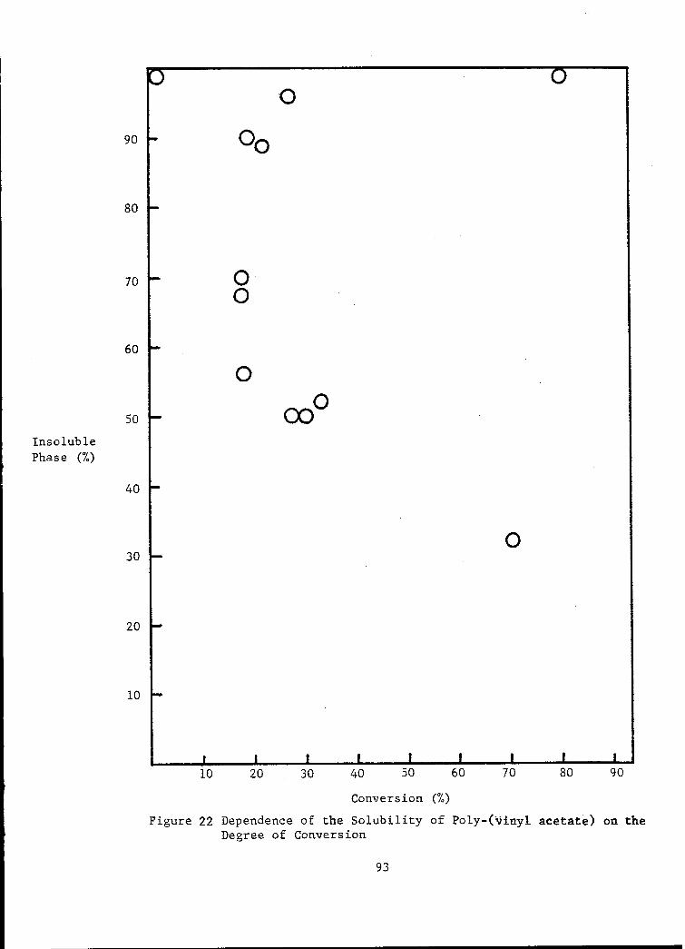
00 0
90 00
80
70 0-0
60
00
50 00InsolublePhase (e)
40
030
20
10
. IIIII I Ii
10 20 30 40 50 60 70 80 90
Conversion (%)
Figure 22 Dependence of the Solubility-of Poly-(•inyl acetate) on theDegree of Conversion
93

D. Summary
Application of the Breuer-Strauss technique of stereospecificpolymerization to emulsions of vinyl acetate stabilized by a bovineserum albumin-sodium dodecyl sulfate complex yields a product whichvaries, depending on the extent of conversionY from an insoluble phasecontaining bound protein at low conversion to a mixture of the in-soluble material and soluble, protein-free polymer at higher conver-sion. The soluble phase is similar in all respects to emulsion PVAcprepared without protein. The insoluble phase exhibits lower rates ofhydrolysis and subsequent reacetylation than the conventional polymer.
94

BIBLIOGRAPHY
1. T. G Fox and S. Loshaek, J. Appl. Phys. 26, 1080 (1955).
2. F. Bueche, J. Chem. Phys. 20, 1959 (1952).
3. F. Bueche, J. Polymer Sci. 43, 527 (1960).
4. P. J. Flory, Principles of Polymer Chemistry, Cornell UniversityPress, Ithaca, New York, 1953, p. 307.
5. P. J. Flory, J. Am. Chem. Soc., 62, 1057 (1940).
6. J. F. Rudd, J. Polymer Sci. 44, 459 (1960).
7. T. G Fox and P. J. Flory, J. Am. Chem. Soc. 70, 2384 (1948).
8. See Chapter 12, pp. 45204 of Rheology, Theory and Applications,Vol. I, F. R. Eirich, Ed., Academic Press, Inc., New York(1956).
9. F. Bueche, J. Polymer Sci. 45, 267 (1960).
10. cf. 8, p. 463-5.
11. cf. 4, p. 340.
12. R. H. Ewart and H. C. Tingey, Abstracts of papers presented at the111th Meeting of the American Chemical Society, Atlantic City,New Jersey, April, 1947.
13. D. C. Pepper, Royal Dublin Soc. 25, 239 (1951).
14. cf. 8, p. 436-7.
15. F. A. Bovey, The Effects of Ionizing Radiation on Natural andSynthetic High Polymers, Interscience Publishers, N. Y., 1958,pp. 74-6.
16. M. Breuer and U. P. Strauss, Private Communication, April, 1960.
17. H. W. Melville and R. R. Sewell, Makromol. Chem., 32, 139 (1959).
18. B. S. Harrap and J. H. Schulman, Disc. for Soc. 13, 197 (1953).
19. G. Strauss and U. P. Strauss, J. Phys. Chem. 62, 1321 (1958).
20. I. Blei, J. Coll. Sci., 15, 370 (1960).
95

PART III - ELASTICITY OF POLYMERIC NETWORKS
I. Specific Diluent Effects on the Elastic Properties of Polymeric Networks- C. A. J. Hoeve and M. O'Brien
A. Introduction
The thermoelastic properties of individual polymeric chains areat present rather well understood. Recent theoretical work' 2 on thechain dimensions as a function of the hindrance to rotation around chainbonds has met with considerable success. For any given force the meanend-to-end distance of the chain may be calculated as a function of tem-perature. However, the thermoelastic properties of networks composed ofsuch chains are much more difficult to comprehend. At first sight rathersweeping assumptions have to be made to enable the construction ofidealized models, for which a theoretical treatment is feasible.
One basic assumption underlying all theories is that the chainsin the unconstrained state are Gaussian. This assumption is not severelyrestrictive and appears to be a good approximation for networks of chainsconsisting of many links.
A second assumption is that interactions between chains areindependent of deformation. This assumption has not yet been evaluatedtheoretically, although some recent experimental evidence 3 suggests thateffects of this nature are not large.
A third assumption is that the unperturbed chain dimensions ofthe free uncrosslinked chains are independent of specific diluent effects.These diluent effects may be important in a study of the elastic propertiesof swollen networks. Contrary to the former two assumptions, the thirdone may be relaxed from a theoretical point of view. The consequences ofthis more general approach are investigated below.
Flory4 has given the following equation for a network in theunswollen state
f = vk T(< 1 >2/L. )(c - a- 2 ). (48)1o
For a network at force zero in swelling equilibrium with a diluent, heobtained4
96

(v V1/NV)[< V >2 v2-v2 /2 ] -[/n(l-v 2 ) + v2 + X1 v2 (49)
and for a force f,)) [<o a >2 /VI2] + XV' 2],
(v V1/NV) [< > (v 3(L IL) - v; 2 1 = -[h(l-vI) + v2 + x(va) (50)
combined with
f = vk T(< a >2 /L ) (v')2/3L~l - L 3 /viES). (51)
2o L -LNILo51
10 10
v is the number of chains in the sample; k and Na are respectivelyBoltzmann's constant and Avogadro's number. T is the absolute temperature.Lio and Li are the lengths of the isotropic sample in the unswollen andswollen state respectively, and L is the length corresponding to the forcef, either for the swollen or unswollen sample. By definition a = L/Lio.v- and v 2 are the volume fractions of polymer in the swollen sample inrespectively the isotropic state and the deformed state, corresponding tof. x' is the interaction parameter for diluent-polymer interaction.V, is the molar volume of the diluent and Vo is the volume of the unswollenpolymer. < 6 >2 = < rf >/< r2 >, where < r' > is the mean square end-to-enddistance of the polymer chains in the isotropic sample at the volume, cor-responding to f, and < ro > is the mean square end-to-end distance foruncrosslinked chains.
2Earlier theories have assumed that < ro > is constant, independent
of temperature and specific diluent effects. However, it has recently3 ' 5
been shown that the temperature dependence of < ro > may be introduced inthe rubber elasticity theory. In fact, at present, this theory is success-fully used to evaluate d in < r2 >/dT for various polymers.
We will now critically examine the implicit assumption that < ro >is independent of diluent effects. The relative probabilities of differentconformations may conceivably depend on the diluent, as has been observedfor 1,2 dichloroethane 6 in different solvents. If these effects alsoexist for polymeric chains, < ro > depends on the diluent. It follows thenthat < a >2, and through eq.(50)the force on an elongated swollen sample, isa function of the diluent.
B. Procedure
The procedure for obtaining the ratio R, defined as < 2 swollen< ro > unswollen' was as follows. From the stress-strain curve in the
97

unswollen state v < X>2 was obtained through eq.(48).Substituting this valueand the measured value of v2 in eq.( 4 9)we obtained )(- Subsequently v 2corresponding to the length L was calculated with the aid of eq(50) and withthis value f was calculated according to eq.(51).During this procedure< ro > was assumed to be equal to < ro > u swollen On comparing the calculatedvalue of the force with that measured at the same L, we have thatR = f /f
calculated measured.
C. Experimental
Linear polyethylene ('Super Dylan", low pressure polyethylene,obtained from the Koppers Company) was chosen as the polymer. The diluentschosen were paraffin, melting range 65-70'C, n-hexadecane, a-chloronaphthaleneand di-2-ethylhexyl azelate. The latter three solvents were "Reagant Grade"and no attempt was made to purify them further.
Polyethylene films of a uniform thickness of 1-2 mm. were pressedat about 150'C and samples were cut at room temperature with a mold in theshape of a dumbbell. These samples are of uniform width of 3.1 mm. over alength of 25 mm. In order to crosslink the samples, they were irradiatedat room temperature in evacuated glass containers by y-radiation from acylindrical Co6 ° source with a uniform dose rate of 0.61 megarep/hr. Thesamples investigated below received doses of 10 to40 megarep. The dumbbellshape enabled the samples to be clamped in and stretched without breakageat the clamps. The clamps consisted of a pair of small metal plates, heldtogether by screws. The lower clamp was fixed, while the upper clamp wassuspended from a strain gauge which could be adjusted vertically. Thestrain gauge (Statham Instrument Company, Transducer Model G-l) had acapacity of 750 g. and a linear response of 0.05 my. per g. under a suppliede.m.f. of 12 v. The output of the strain gauge was displayed on a Leedsand Northrup recorder, giving a full scale deflection of 10 mv. The instru-ment was calibrated by addition of known weights before and after eachexperiment.
The length of the sample was measured with a cathetometer. Twothin metal pins, perforating the uniform section 20 mm. apart, served asmarkers.
A stream of high purity nitrogen was passed through the samplechamber in order to prevent oxidative degradation. Samples were swollenby diluent in the sample chamber. After the stress-strain experiment, thepolyethylene sample was extracted with boiling xylene and evaporated todryness at 150°C in vacuum. The stress-strain curve in the unswollenstate after this treatment was usually identical, within experimentalerror, to that before swelling; otherwise the experiment was discarded.
The liquid thermostat (containing Silicone Oil DC-550, DowCorning Corporation) maintained a constant temperature of 150 ± O.I°C.
Stress-strain curves were obtained by stretching the sample atintervals to an extension ratio of about 1.3 and decreasing the length in
98
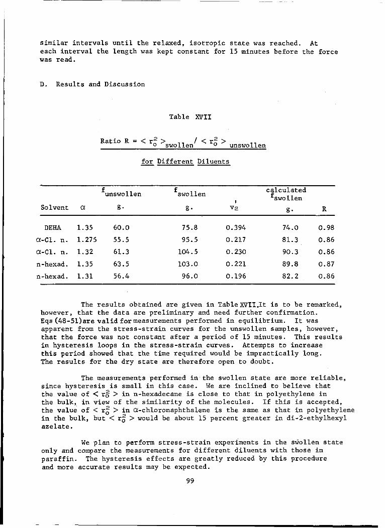
similar intervals until the relaxed, isotropic state was reached. Ateach interval the length was kept constant for 15 minutes before the forcewas read.
D. Results and Discussion
Table XVII
RatioR 2 >swo < r2 >0 Swollen 0 unswollen
for Different Diluents
f f calculatedunswollen swollen fswollen
Solvent a g. g. v 2 g. R
DEHA 1.35 60.0 75.8 0.394 74.0 0.98
a-Cl. n. 1.275 55.5 95.5 0.217 81.3 0.86
a-Cl. n. 1.32 61.3 104.5 0.230 90.3 0.86
n-hexad. 1.35 63.5 103.0 0.221 89.8 0.87
n-hexad. 1.31 56.4 96.0 0.196 82.2 0.86
The results obtained are given in Table XVII.It is to be remarked,however, that the data are preliminary and need further confirmation.Eqs (48-51)are valid formeasurements performed in equilibrium. It wasapparent from the stress-strain curves for the unswollen samples, however,that the force was not constant after a period of 15 minutes. This resultsin hysteresis loops in the stress-strain curves. Attempts to increasethis period showed that the time required would be impractically long.The results for the dry state are therefore open to doubt.
The measurements performed in the swollen state are more reliable,since hysteresis is small in this case. We are inclined to believe thatthe value of < ro > in n-hexadecane is close to that in polyethylene inthe bulk, in view of the similarity of the molecules. If this is accepted,the value of < ro2 > in a-chloronaphthalene is the same as that in polyethylenein the bulk, but < r2 > would be about 15 percent greater in di-2-ethylhexylazelate.
We plan to perform stress-strain experiments in the swollen stateonly and compare the measurements for different diluents with those inparaffin. The hysteresis effects are greatly reduced by this procedureand more accurate results may be expected.
99
BIBLIOGRAPHY
1. C. A. J. Hoeve, J. Chem. Phys., 32, 888 (1960).
2. C. A. J. Hoeve, J. Chem. Phys., in press.
3. A. Ciferri, C. A. J. Hoeve and P. J. Flory, J. Am. Chem. Soc.,83, 1015 (1961).
4. P. J. Flory, J. Am. Chem. Soc., 78, 5222 (1956).
5. P. J. Flory, C. A. J. Hoeve and A. Ciferri, J. Polymer Sci.,34, 337 (1959).
6. M. V. Volkenstein and V. I. Brevdo, Zhur. Fiz. Khim. 28,1313 (1954); Y. H. Inami, J. B. Ramsey, J. Chem. Phys.31, 1297 (1959).
100
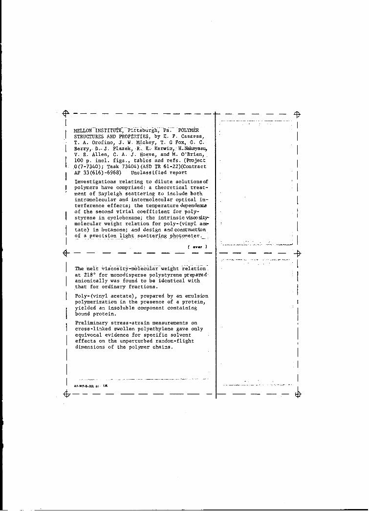
MELLON INSTITUTE, Pittsburgh,- Pa.--- POLYMERSTRUCTURES AND PROPERTIES, by E. F. Casassa,T. A. Orofino, J. W. Mickey, T. G Fox, G. C.Berry, D.-J. Plazek, R. E;* Kerwiny:H.Nakayas;V. R. Allen, C. A. J. Hoeve, and M. O'Brien,100 p. incl. figs., tables and refs. (Project0(7-7340); Task 73404)(ASD TR 61-22)(ContractAF 33(616)-6968) Unclassified report
Investigations relating to dilute solutionsofpolymers have comprised: a theoretical treat-ment of Rayleigh scattering to include bothintramolecular and intermolecular optical in-terference effeccs; the temperature dependenceof the second virial coefficient for poly-styrene in cyclohexane; the intrinsic viscosty-molecular weight relation for poly-(vinyl ac-tate) in butanone; and design and constnuctionof a precision light scattering photometer.
C oVO, I
The meit viscosity-molecular weight relation.at 218' for monodisperse polystyrene preparedanionically was found to be identical withthat for ordinary fractions.
Poly-(vinyl acetate), prepared by an emulsionpolymerization in the presence of a protein,yielded an insoluble component containingbound protein.
Preliminary stress-strain measurements oncross-linked swollen polyethylene gave onlyequivocal evidence for specific solventeffects on the unperturbed random-flightdimensions of the polymer chains.
AF-WP-8-JUL 61 IM