Polymer Artificial Muscles - Worcester Polytechnic Institute · world-class research environment at...
90
Polymer Artificial Muscles Controls and Applications with Low-Cost Twist Insertion Fiber Actuators A Major Qualifying Project Submitted to the Faculty of Worcester Polytechnic Institute in partial fulfillment of the requirements for the Degree of Bachelor of Science in Robotics Engineering By ____________________________________ William Hunt Robotics Engineering Program Date: 6 May 2015 Project Advisor: ____________________________________ Professor Cagdas Onal This report represents the work of a WPI undergraduate student submitted to the faculty as evidence of a degree requirement. WPI routinely publishes these reports on its web site without editorial or peer review. For more information about the projects program at WPI, see http://www.wpi.edu/Academics/Projects.
Transcript of Polymer Artificial Muscles - Worcester Polytechnic Institute · world-class research environment at...

Polymer Artificial Muscles Controls and Applications with Low-Cost Twist Insertion Fiber Actuators
A Major Qualifying Project
Submitted to the Faculty of Worcester Polytechnic Institute
in partial fulfillment of the requirements for the
Degree of Bachelor of Science in Robotics Engineering
By
____________________________________
William Hunt
Robotics Engineering Program
Date: 6 May 2015
Project Advisor:
____________________________________
Professor Cagdas Onal
This report represents the work of a WPI undergraduate student submitted to the faculty as
evidence of a degree requirement. WPI routinely publishes these reports on its web site without
editorial or peer review. For more information about the projects program at WPI, see
http://www.wpi.edu/Academics/Projects.
ii
Abstract
Functional artificial muscle fibers could reduce the cost, weight and complexity of many robotic
systems, and are therefore an attractive development goal in robotics engineering. When coiled
into flexible helical artificial muscle fibers, Nylon monofilaments produce linear tensile
actuation under thermal stimulus. In this research the behavior of these coiled muscle fibers was
investigated using a test fixture designed to emulate the conditions in a real application. Tests
showed muscle performance consistent with past research, but also revealed a previously
undocumented thermal effect wherein muscles changed length unexpectedly under variable-
loading conditions at high temperatures. This effect, along with other known properties of the
muscle fibers, was modeled in a parametric simulation environment, and parameter estimation
utilities were used to quantitatively match the model to the real-world response. The matched
parameter model was used to simulate a computer controlled antagonistic servo-joint, which
illustrated the potential of the muscle fibers for real-world application, and the controls
challenges introduced by the newly discovered thermal effect.

iii
Acknowledgements
It is difficult to thoroughly document the network of exceptional individuals who maintain the
world-class research environment at Worcester Polytechnic Institute. The author Mr. Hunt
wishes to express particular gratitude for the continuing assistance of advisor Prof. Cagdas Onal,
along with his doctoral research staff in the WPI Soft Robotics Laboratory. Special thanks are
extended to Arthur C. Heinricher at WPI, for his ongoing encouragement and support of the
author’s work leading up to this project.
Additional thanks to:
E.A. Partlow III, Cornell University
R. Baughman, U.T. Dallas
Washburn Laboratories, WPI
T. Chaulk & J. Johnson, WPI
P. Radhakrishnan, WPI

iv
Contents
1 Introduction ............................................................................................................................. 1
1.1 Basis for this Research ..................................................................................................... 1
1.2 Contributions to the Field ................................................................................................. 2
2 Background .............................................................................................................................. 2
2.1 Muscle Applications in Robotics ..................................................................................... 2
2.2 Past Work in Artificial Muscles ....................................................................................... 4
2.3 Twist-Insertion Polymer Muscles .................................................................................... 6
2.4 Twist Mechanics and Anisotropism ................................................................................. 8
2.5 Achieving Linear Actuation ............................................................................................. 9
3 Methods ................................................................................................................................. 10
3.1 Method of Fiber Generation ........................................................................................... 10
3.2 Preliminary Characterizations ........................................................................................ 12
3.3 Design of Antagonistic Configuration ........................................................................... 18
3.4 Rotary Fixture Characterization ..................................................................................... 22
3.5 Parametric Modeling ...................................................................................................... 25
3.6 Controls for Antagonistic Configuration........................................................................ 27
4 Results ................................................................................................................................... 27
4.1 Preliminary Test Findings .............................................................................................. 27
4.2 Model Findings .............................................................................................................. 36

v
4.3 Parameter Estimation Findings ...................................................................................... 45
4.4 Controls Findings ........................................................................................................... 52
5 Discussion and Conclusions .................................................................................................. 58
5.1 Application Notes ........................................................................................................... 58
5.2 Further Research ............................................................................................................ 60
5.3 Project Conclusion ......................................................................................................... 62
6 References ............................................................................................................................. 63
APPENDIX A Antagonistic Stimulus Fixture Design Documents ......................................... 65
APPENDIX B Antagonistic Stimulus Fixture Software.......................................................... 76
APPENDIX C Antagonistic Stimulus Fixture Operating Instructions .................................... 83

1
1 INTRODUCTION
1.1 BASIS FOR THIS RESEARCH
There are a number of robotic applications for low-cost muscle-like actuators, especially in
rapidly developing fields such as humanoid control, active prosthetic design and wearable textile
devices [5]. Artificial muscle technologies could lead to an era of dramatically increased human-
robot interaction and integration, wherein humans receive replacement artificial muscle implants,
and robots become just as nimble and dexterous as their human designers [29].
Haines et al. have demonstrated a novel approach for synthesizing artificial muscle-like actuator
fibers from commercially available, low-cost polymer fibers such as fishing line by twist
insertion. These fibers exhibit contraction of up to 49%, with considerable load capacity and very
low hysteresis. They offer cost, simplicity, weight and strength advantages over a number of
existing technologies. In particular, they possess a high strength-to-weight ratio, making them
potentially valuable in aerospace applications. Several example configurations for the application
of these fibers have already been demonstrated, including textile-woven, braided, plied and
bundled actuators, driven electro- and hydro-thermally [5].
This project investigates robotic design applications and limitations for the polymer muscle
fibers of Haines et al. in research and development phases. First, elements of muscle fiber
production are reproduced. Next, a prototype actuator configuration is developed, and used to
perform an assay of non-repeatable elements in muscle actuation, and the resulting limitations on
muscle control. Finally, a controlled model for a 1-DOF rotational robotic joint (based upon the
prototype actuator configuration) is produced in-silico. The dynamical characteristics of this
simulated joint are documented, and potential applications are discussed.
2
1.2 CONTRIBUTIONS TO THE FIELD
This project attempts to recreate the helical muscle fibers of Haines et al., characterize some of
their behavioral properties, and demonstrate a prototype antagonistic rotary actuator
configuration in-silico, using Joule heating and passive cooling. The end result and primary
robotic design component of this project is a rotational joint fixture that can be driven by
antagonistically biased (prestrained) muscle fibers, and which may be used by a future project
group to implement the simulated joint from this project. This joint illustrates the applicability of
twist-insertion fiber actuators to controlled robots, and reveals the limitations of the actuators. As
such, this work also provides an outline for future research in soft robotic actuation systems,
especially those that require high work capacity, including aerospace, micro- and nano-robots,
and ultra-low-cost systems.
2 BACKGROUND
2.1 MUSCLE APPLICATIONS IN ROBOTICS
Many robotics applications require control of the position and/or dynamical characteristics of a
mechanism. There is widespread interest in a category of actuators that behave similarly to
natural muscle fibers, affording positional, force and/or impedance control while maintaining a
flexible, lightweight form factor. Artificial muscle technologies are an attractive solution to
challenging robotics problems, especially in robots such as humanoids, manipulators and
prostheses [5]. Artificial muscles may also be useful in aerospace, as they provide a light-weight
alternative to existing transducer technology. Contrary to traditional cost- and weight-expensive
geared motors, artificial muscle systems have the potential to be both physically and
operationally flexible, and customizable for a wide range of applications [29].

3
Pneumatic muscle systems are already known to be well suited for complicated open-chain
robots [10]; these systems have been used in various robots including humanoid walking systems
[19] and dexterous graspers [27]. Force application contexts that preclude more traditional
actuators due to weight, noise or cost are good potential applications for pneumatic muscles. For
example, Serres [16] showed an application for pneumatic muscles in human resistive strength
training under orbital microgravity.
Natural muscles operate in antagonistic pairs or groups, which afford precise control of
movement [1]. Human motion is dependent upon the dynamical characteristics of these muscle
groups. Modern walking prostheses seek to
emulate the properties of natural limbs,
which can dynamically adjust mechanical
joint impedance properties [11]. While
existing systems such as hysteresis brakes
and series elastic actuators allow this type of
control, these technologies can be
cumbersome and expensive. Artificial
muscle systems may solve this problem in a
more compact, comfortable package [11].
Developers of walking and humanoid robots
have attempted to emulate the dynamical
properties of natural muscle groups [18].
Artificial muscles are likely to improve the
realism of these bio-mimetic designs,
Fig. 1: Atlas, a modern humanoid robot, image credit WPI via DARPA [25]

4
because these actuators typically operate in antagonistic groups [10]. Complicated movements
such as walking have already been achieved using this approach [19].
Artificial muscles have been applied in non-traditional applications. Madden et al. [14] provided
case studies detailing naval-specific muscle applications for controlling the shape and orientation
of propeller blades. An example variable-camber propeller was proposed for the Expendable,
Mobile Antisubmarine Warfare Training Target (EMATT) vehicle, and some existing artificial
muscle technologies were shown to be feasible actuation systems for this design [14]. Because of
their light weight, artificial muscles could also be valuable in aerospace systems.
2.2 PAST WORK IN ARTIFICIAL MUSCLES
Artificial muscle research has spanned various technologies, many of which are based around
specialized materials. In some cases, esoteric alloys, polymers and gels have been shown to
exhibit muscle-like behavior. In other cases, more conventional materials and technologies have
been formed into macroscopic structure that create the desired behavior. Artificial muscle
research draws heavily on the findings of materials science and nanotechnology scholars.
Perhaps the most conventional and well-known artificial muscle technology is the pneumatic or
McKibben air muscle [2]. A pneumatic muscle is constructed by containing an airtight, flexible
tube or bladder within a braided, non-
extensible fiber shell. When the bladder is
inflated, the shell converts the inflating
pressure into a compressive or tensile
force along the length of the muscle,
resulting in displacement and/or force
Fig. 2: Robotic hand using air muscles, image credit Shadow Robot Company [26]
5
application. These actuators are strong and light, but (like other fluidic actuators) they require
pressure and valve systems [2].
As noted above, pneumatic muscles have seen significant adoption [10][19][27][16]. One
application, a dexterous hand from the Shadow Robot Company, is shown in Fig. 2 [26].
Existing applications for pneumatic muscles may benefit from the introduction of more advanced
muscle-like actuators that do not require fluidic control overhead.
Relatively common material-based artificial muscle technologies are based around shape
memory alloys (SMAs), which include the well-known Nitinol (a nickel-titanium alloy). SMAs
can be formed into muscle-like devices that actuate with temperature [13]. SMA products are
commercialized and broadly available for muscle applications. An example product is Flexinol
actuator wire, available from Dynalloy, Inc. [9]. Flexinol is a Nitinol variant, capable of up to
7% reversible stroke with a muscle strength that exceeds the yield strength of the alloy at
operating temperature (a Flexinol wire can exert enough force to break itself).
SMAs have convenient features such as intrinsic conductivity, which permits direct
electrothermal heating. Unfortunately, while they can provide fast, high energy strokes, SMAs
are highly hysteretic and therefore difficult to control [5][13]. SMAs are also expensive when
used in large quantities to achieve high-strength actuation: the cost of Flexinol wire actuators
exceeds $700 US per kilogram [8].
Shape Memory Polymers (SMPs) provide similar functionality to SMAs, but at a lower strength,
cost and weight. They are not inherently conductive, so they are harder to heat than Nitinol and
its variants [17]. Fiber reinforcement provides some improvement in SMP strength [17], and

6
researchers showed that performance improved when SMPs were filled with carbon nanotubes
[12].
Another polymer solution uses an electroactive approach, in which dielectric elastomers are
subjected to electric fields [24]. This Electro-active Polymer (EAP) technology does not require
heating for actuation, but necessitates a high voltage [5][24]. Some other electroactive polymers
need to be stimulated chemically or electrochemically, in a wet environment, or are themselves
gels [11]. These technologies have exhibited relatively high efficiencies (~20%), but impose the
additional system load of chemical storage and delivery [11].
Carbon nanotubes (CNTs) can be spun into yarns, which provide torsional and linear actuation
under appropriate conditions [15][20]. These types of actuation can be induced by multiple
stimulation methods, including electrochemical charge injection [15], gas absorption on an
attached layer of palladium and thermal changes [20]. Thermal actuation was achieved by
infiltrating the CNT yarn with a guest such as wax. When made to expand and contract under
changes in temperature (which can be produced using light or electricity), wax-infiltrated yarns
provided lengthwise actuation on the order of 5%, with a unit-mass work capacity up to 29 times
that of a natural muscle [20]. Unfortunately these muscles rely on state-of-the-art carbon
nanotube technology and are therefore expensive [5].
2.3 TWIST-INSERTION POLYMER MUSCLES
Recent work by Haines et al. demonstrated a novel form for a thermo-mechanical artificial
muscle based on low-cost, readily available precursor materials. The seminal work in Science [5]
explained a process of twist insertion into drawn fibers of nylon (and similar materials).

7
When the twisted fibers are heated, they untwist,
producing strong torsional actuation. If these
same fibers are coiled into helical spring-like
strands (as shown in Fig. 3), heating induces
linear contraction along the helix axis. Haines et
al. provided an overview of the characteristics of these actuator strands, and illustrated various
example configurations including parallel linear actuators, braids and textiles. Twist insertion
actuators have a work capacity, relative to mass, over 100 times that of natural human muscle
[5], which is a three-fold improvement over the expensive carbon nanotube technology discussed
above [20]. The coiled fibers exhibited very low hysteresis performance and sustained one
million cycles of operation, but exhibited low maximum energy conversion efficiencies on the
order of 1% [5].
In the original research, electro-thermal actuation was obtained using Joule heating in filaments
pre-coated with conductive material, or by twisting a discrete conductive element into the fiber
during fabrication. Hydro-thermal heating was also achieved by containing muscle fibers within
a fluid-tight tube, which was alternately filled with hot and cold water to cycle the muscle [5]. In
more recent research, fibers were painted with conductive silver paint before coiling. The silver
paint then provided the electrical pathway for Joule heating. These silver-plated filament
actuators cycled more quickly when cooled passively in water [25].
In some of the tests of Haines et al., coiling was induced by continuous twisting of the fiber, to
the point that the fiber began to twist around itself helically (a phenomenon known as writhe). In
other tests, twisted fibers were wrapped around mandrels of various diameters. This produced
Fig. 3: Optical image of coiled nylon fiber actuator

8
muscles capable of greater actuation distance, but lower load capacity, a geometrically intuitive
result [5].
Twist insertion muscles are extremely easy to manufacture, requiring only a rotating spindle and
a means to keep the coiling fiber under tension. Media coverage of this technology has
highlighted the ease of manufacturing from common fibers such as fishing line and sewing
monofilament, and even encouraged hobbyists to pursue their own applications [6].
2.4 TWIST MECHANICS AND ANISOTROPISM
Haines et al. describe the thermal expansion of drawn polymer fibers, which can be anisotropic
(an important property if mechanical twisting action is required) [5]. Aligned crystalline regions
of polymer samples have negative thermal expansion along the chain direction, due to a
hypothesized change in the rotation of carbon-carbon bonds within the polymer backbone [30].
Drawn fibers that are not entirely crystalline can exhibit a much greater lengthwise contraction
than purely aligned crystalline molecules, because of the contraction of amorphous elastic tie
molecules within the fiber structure [4][3]. These drawn fibers also expand diametrically, due to
the expansion of crystalline regions [25][4]. The result is an anisotropic expansion, with a
negative coefficient in the draw direction and a positive coefficient perpendicular thereto.
Torsional untwisting occurs when twisted polymers that exhibit these anisotropic expansion
conditions are heated. When a fiber is twisted, the polymer chains oriented lengthwise along the
fiber form helices. Shrinking in polymer chains now occurs along these helices. Haines et al.
describe an analogous relationship between original fiber length, twist, axial length and diameter
in the surface layer of a yarn [4]:
Δ𝑛
𝑛=Δ𝜆
𝜆
1
cos2 𝛼𝑓−Δ𝑑
𝑑−Δ𝑙
𝑙tan2𝛼𝑓 (1)

9
In this expression, 𝑛 is the fiber twist, 𝜆 the polymer chain length, 𝑙 the twisted fiber length, 𝛼𝑓
the angle of the molecular helix formed by twisting, 𝑑 the original fiber diameter, and Δ-
expressions the temperature-induced changes in these quantities. By this analogy, Haines et al.
explained that a change in twist is related to lengthwise fiber contraction and diametric fiber
expansion. As equation (1) illustrates, these two effects combine additively to affect torsional
action. This leads to a useful conjecture: it is advantageous in twist-insertion muscle design to
select precursor fibers with highly anisotropic thermal expansion characteristics, in which a
temperature increase causes the fiber to contract lengthwise and expand diametrically [5][4].
2.5 ACHIEVING LINEAR ACTUATION
The linear actuation achieved by helical fiber configurations is explained by the fiber untwisting
effect described in the previous section. A fiber that has been coiled into a helix will undergo
twisting when the helix is extended and compressed. The magnitude of this twisting is described
by this equation, from Haines et al. [5]:
Δ𝑇 =𝑁Δ𝐿
𝑙2 (2)
Where 𝑙 is the length of the original, fiber, Δ𝐿 is the change in length of the helical coil, 𝑁 is the
number of coils and Δ𝑇 is the change in twist per unit length in the original fiber. Equation (2) is
fundamentally a formulation of spring mechanics [5][25][4]; it illustrates that a change in fiber
twist will produce a corresponding, proportional change in helix length. By comparison of the
mechanical work achieved by torsional and linear twist-insertion actuators, Haines et al.
demonstrated empirically that the twist-length relationship of equation (2) is likely to be the
mechanism that drives linear actuation in coiled muscle fibers [5].

10
3 METHODS
3.1 METHOD OF FIBER GENERATION
A simple test and manufacturing fixture was developed to produce and characterize the twist
insertion muscle fibers investigated by Haines et al.
[5]. The twisting fixture comprised a benchtop
twisting stand, a heat gun for muscle stimulation,
and a digital camera for recording tests. The stand
provided a convenient USB serial port user interface,
controlled twist insertion, and a weight hook for
gravitational tension application. Bags of small ball
bearings, measured on scales, served as calibrated
weights. Fig. 4 shows the fiber twisting and test
stand CAD model.
The tabletop test stand was only capable of twisting
short lengths of muscle fiber, and could not twist
muscles quickly. Thus, this fixture was dismantled
for parts midway through the project period, and
replaced by a less formal setup permitting rapid preparation of longer samples. A metal wire
hook was installed in the chuck of a handheld electric drill. Nylon fiber tied to this hook was
weighted to calibrated tensions by the same technique used for short lengths (a metal hook with a
bag of weighted ball bearings). Longer fibers were coiled using existing vertical drops such as
balconies and stairwells. For such large sample lengths, zip ties were attached to the weighted
Fig. 4: Computer-aided design graphic for muscle twisting fixture
11
end of the twisting fiber and permitted to ride against a vertical wall or board to prevent
unwinding.
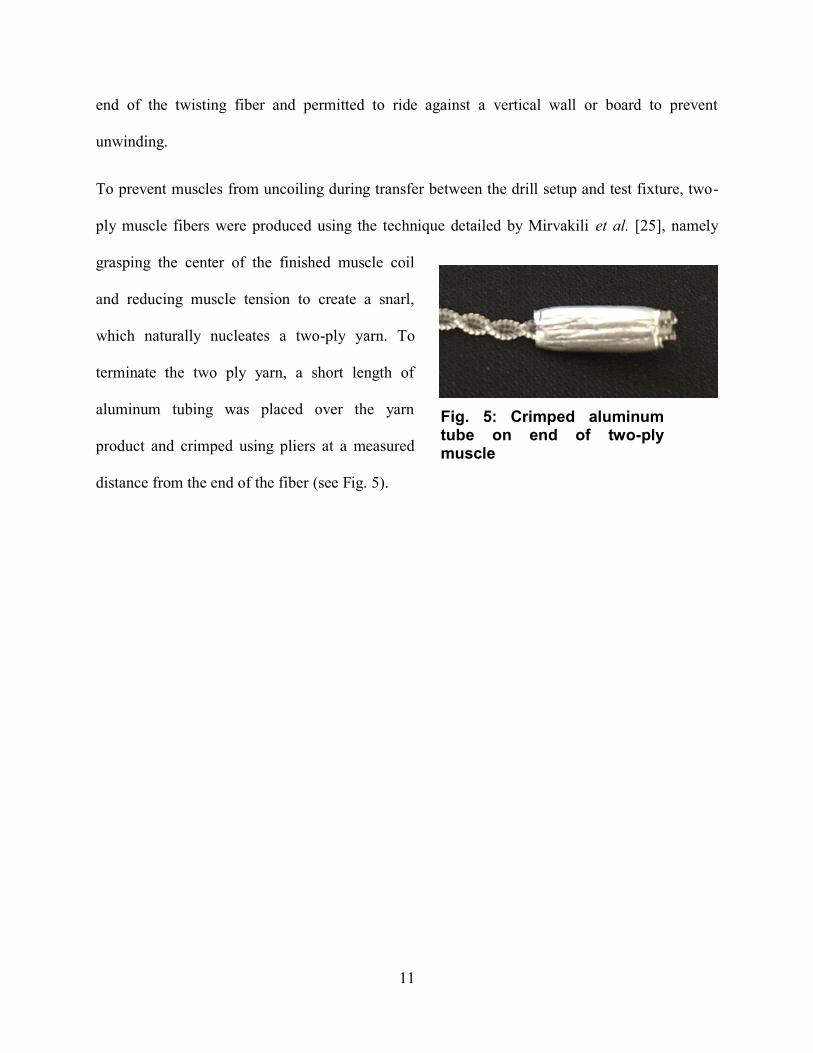
To prevent muscles from uncoiling during transfer between the drill setup and test fixture, two-
ply muscle fibers were produced using the technique detailed by Mirvakili et al. [25], namely
grasping the center of the finished muscle coil
and reducing muscle tension to create a snarl,
which naturally nucleates a two-ply yarn. To
terminate the two ply yarn, a short length of
aluminum tubing was placed over the yarn
product and crimped using pliers at a measured
distance from the end of the fiber (see Fig. 5).
Fig. 5: Crimped aluminum tube on end of two-ply muscle

12
3.2 PRELIMINARY CHARACTERIZATIONS
The seminal research [5] illustrated that a wide range of spring indices could be achieved in the
test fiber by nucleating coils at a common load and subsequently changing to a smaller or larger
load, depending on the spring index desired. To reduce the number of variables at play and
simplify the twist insertion process, this research addressed only artificial muscle fibers produced
using a fixed load. Fiber characterization testing began with a series of coiling operations using a
few different fiber diameters and coiling loads, to establish the range of loads that nucleated
suitable coils in different diameter fibers.
Note that only a small selection of precursors was considered during this test, due to limitations
on time for testing. The preliminary tests addressed here were performed on muscles coiled from
2-lb, 12-lb and 20-lb grades of a single example precursor product: Trilene XL Smooth Casting
monofilament fishing line. As noted in the seminal research [5], twisted nylon actuators seem to
exhibit common scale-independent behaviors, so it is reasonable to expect that the effects
observed here will also occur when alternative precursor test ratings are used.
The procedure for static characterization required a very simple setup. A muscle was coiled on
the test rig of Fig. 4 and loaded with a mass of known weight. It was then brought to a high
temperature using a heat gun, and allowed to cool. At each step of heating and cooling, the
temperature of the muscle was verified using a thermocouple, and an image was captured. This
process of cycling was repeated several times, to “train” the muscle. After that point, the muscle
was brought to a series of different temperatures (controlled by manually changing the distance

13
to the heat gun), and images were captures at each step. Finally, the images collected during the
test were analyzed in the program Kinovea1 to determine the length of the fiber at each test point.
Note that the process of cycling the muscle to a high temperature was only added after a failed
attempt at characterization illustrated a “training” effect. Whenever the load changed, cycling to
high temperatures caused permanent deformation that did not reverse during cooling. By
repeatedly cycling the muscle to a high temperature, it was possible to illustrate a condition of
repeatable actuation.
The earliest characterization tests revealed a complex training effect, which prevented a basic
model of muscle behavior from being established. To produce a more model-suggestive dataset,
it was necessary to perform more elaborate series of tests, here dubbed the “detailed
characterization”. Detailed characterization was split into two test sequences, referenced here as
T1 and T2.
The preliminary tests used a heat gun as a heat source, requiring a great deal of user input and
control. The heat gun test rig was extremely slow and provided poor quality data points due to its
lack of precise thermal control. It was determined to be inadequate for detailed characterizations.
To mitigate this problem, various electrical heating systems were explored.
If the muscle was wrapped in a fine resistive wire, and the wire heated by an electric current, the
muscle would theoretically take on the temperature of the wire after a certain period. When
tested practically, however, the hot wire always formed a knife-like cutting edge and sliced
through the muscle. Even a small indentation in the muscle fiber surface would be enough to
nucleate further splitting, so it is reasonable that the hot-wire approach was impractical. A
1 http://www.kinovea.org/
14
similar effect was observed when a multi-fiber conductive thread element was used in place of
the hot wire. While the conductive thread element provided more diffuse heat, it still localized
heating enough to cut through the fiber.
Haines et al. [5] demonstrated a mode of uniform surface-layer heating using pre-plated silver
fibers. Those precursor fibers were not obtained in time for testing. A similar technique of [5]
dictated that the muscle be wrapped in forest-grown carbon nanotube sheet, which formed a
flexible conductive layer. This was similarly impractical within the scope of this project.
Mirvakili et al. [25] demonstrated a technique for reproducing the surface-layer heaters of [5], in
which a conductive silver bearing paint was applied to the muscle surface at some point during
manufacturing. An advantage to this method is the ability to apply the paint at any stage; e.g.
mid-twisting but before supercoiling (the preferred technique in [25]), which theoretically
reduces the amount of flexibility required. The paint used in [25] was SPI Flash-Dry, a very
expensive compound intended for electrically conductive sample mounting. As a less expensive
substitute, a vial of Ted Pella, Inc. Pelco Conductive Silver Paint was obtained.
At first, the muscle was painted during the coiling process, just before supercoiling. The Pelco
paint proved insufficiently flexible, incrementally flaking off the muscle fiber during
supercoiling. Next the paint was experimentally applied after coiling, to the entire muscle coil
structure, using a foam applicator pad. This produced an effective surface heating element, but
that element soon flaked away during muscle operation. At this point, the paint technique was
abandoned due to the high cost of silver paint samples. Further testing used a more complex, but
less expensive, alternative. It is recommended that future experimenters attempt to obtain pre-
plated precursor fibers or the proper SPI Flash-Dry paint compound, in order to reproduce the
heating elements from [5] and/or [25].

15
The low-cost heating alternative comprised a small-
diameter tubular diffuser device. The heater itself
comprised an aluminum tube, wrapped in Kapton tape, and
subsequently in Kanthal heating wire. The selected tube’s
diameter was just large enough to accommodate a test
muscle. Tubes constructed from kitchen-grade aluminum
foil were tested and shown to be effective, but solid
aluminum tubes with a greater wall thickness were stronger
and easier to re-use. This design produced a uniform heated
environment for the muscle, at the cost of high-speed
heating and cooling (the heater tube diffuser introduced a
large amount of extra thermal mass).
In the case of the preliminary tests, the tube was made long
enough to completely contain the sample muscle fiber,
Because the tube obscured the muscle’s length and
prevented direct weight attachment, a wire hanger was produced that fit inside of the tubular
heater. This wire was attached to the end of the sample, and a weight hanger and anti-rotation
moment arm were formed at the other end. Additionally, a circular vision target was affixed to
the hanger, to simplify analysis of test images. An electrical current was applied to the Kanthal
wire to increase the temperature of the muscle tube. An external, manually-controlled fan was
sometimes used during cooling to speed up the tests.
The driver circuit for the heater was an older, single channel version of the circuit developed for
the antagonistic test fixture, which is documented in Section 3.3. The original driver circuit was
Fig. 6: Detail Test Setup
16
destroyed during transportation of the test setup, but the circuit for the antagonistic test fixture
was designed to be compatible with the T1/T2 heater setup. Further documentation for that
circuit is omitted here, as it is thoroughly documented in Section 3.3. Similarly, the computer
program interface for the heater controller (a PI controller with a feedforward component) was
very similar to that for the antagonistic fixture, also documented in Section 3.3. That program is
omitted from this report, as it is merely an early version of the antagonistic fixture program, with
slower logging and only a single channel of control. Note that this project did not use any source
control repository or formal versioning, because the number of software tools developed was so
small.
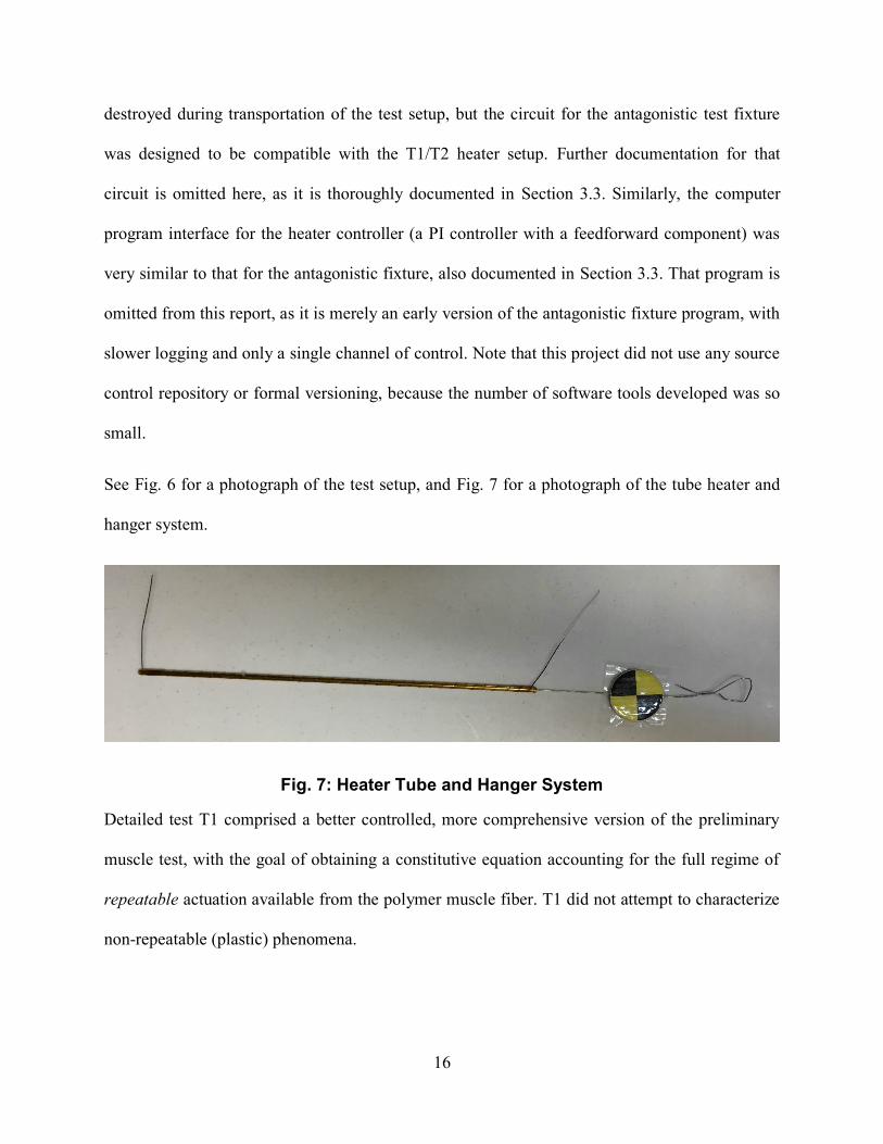
See Fig. 6 for a photograph of the test setup, and Fig. 7 for a photograph of the tube heater and
hanger system.
Fig. 7: Heater Tube and Hanger System
Detailed test T1 comprised a better controlled, more comprehensive version of the preliminary
muscle test, with the goal of obtaining a constitutive equation accounting for the full regime of
repeatable actuation available from the polymer muscle fiber. T1 did not attempt to characterize
non-repeatable (plastic) phenomena.
17
A sample two-ply muscle was loaded into the heater tube, and a small weight of 275 g was
applied. The heater was then cycled to a high temperature (90°C) and returned to room
temperature (approximately 25°C) five times. After cycling, muscle fiber temperature was swept
through a series of increasing values, and finally returned to room temperature. At this point, the
load on the muscle was increased, and the process repeated.
This was the extent of testing performed in the preliminary phase. For T1, though, additional
data points were collected; after the first batch of data, a series of five additional batches were
collected. The procedures for these batches were identical, but in each new batch, the peak
temperature used during initial cycling was reduced. In an attempt to prevent previous tests from
influencing each new batch, the muscle was cycled five times to 90 degrees at the 275 g load
between batches.
To communicate the basis for test T2, a brief digression into the results of T1 is necessary. T1
demonstrated that muscle actuation could be described using two quantities in superposition, first
an actuation descriptor 𝑐, and second a deformation descriptor 𝑠. The actuation descriptor
appeared to be an instantaneous function of muscle temperature, while the deformation 𝑠
appeared to depend on the muscle’s historical temperature and load parameters. In short, the
parameter 𝑠 accounted for plastic deformation and nonlinear dynamic effects.
Originally, test T2 was intended to produce a thorough characterization of the behavior of
parameter 𝑠 and therefore the hysteretic element of the muscle constitutive model. Unfortunately,
time did not permit such a complete characterization. Instead, a slice of the sample space was
collected using the following regime:
T2.i Cycle to a high temperature at a low load (90°C, 275 g).
T2.ii Cool to a low temperature (25°C, 275 g).

18
T2.iii Change load to a “starting load” parameter (25°C, starting load).
T2.iv Heat to a “starting temperature” parameter (starting temperature, starting load).
T2.v Cool to low temperature (25°C, starting load).
T2.vi Change to “ending load” parameter (25°C, ending load).
T2.vii Heat to “ending temperature” parameter (ending temperature, ending load).
T2.viii Heat to high temperature (90°C, ending load).
T2.ix Change load to low load (90°, 275 g).
T2.x Start over at step T2.ii with a new set of load and temperature parameters; repeat for
various parameter permutations.
These tests were performed at a set of loads (700 g, 850 g, 1000 g, 1150 g) and temperatures
(25°C, 50°C, 70°C, 90°C) in each available permutation of starting load, ending load, starting
temperature, and ending temperature. Accounting for small amounts of data lost due to testing
error, 250 of the available 256 permutations were successfully captured. The structure of these
tests permitted deduction of the behavior of the 𝑠 parameter during heating from room
temperature, after training to many different sets of loads and temperatures.
Because the heating processes in T2 were only performed starting at room temperature, T2 did
not generate a comprehensive constitutive equation for plastic deformation behavior. Complete
tests would need to assess the effect of changing both temperature and load, without returning to
room temperature in between events. Nevertheless, T2 illustrated the degree of plastic
deformation possible during muscle operation within a wide range of temperatures, and was
therefore informative of broad quantitative conclusions about muscle control and application
limitations.
3.3 DESIGN OF ANTAGONISTIC CONFIGURATION
The antagonistic test configuration was designed to permit testing in a realistic use case, where
the muscle under test drives a rotor whose position may be monitored. The configuration needed
a rotor with attachment points at various radii, a stator with adjustable attachment points, and a

19
low-resistance means for monitoring the position
of the rotor. A final feature requirement was added
to simplify the application of torque: a disc of
constant radius from which a weight-bearing cable
can be suspended, attached to the rotor and
concentric with the axis of rotation.
Both springs and muscles could be used as
antagonistic force elements, in various
configurations. The ends of two-ply muscles are easily looped through their own twists to form
tightening loops. Extension springs also include loops for
mounting. Thus, steel pins (as shown in Fig. 8) provided a
convenient connection means for both these forms of stimulus.
These pins could be easily supported by drilled holes, so a
“pegboard” arrangement of mounting holes was included in
the fixture to satisfy the requirement for adjustable mounting
locations.
To measure the position of the rotor, a low friction Vishay
Spectrol potentiometer was purchased. Rigid mounting of the
potentiometer was not acceptable, as even the slightest
misalignment of the shafts would introduce binding. Instead, a
method similar to patent US 2937861 [23] was adapted to the
design. The potentiometer was mounted to a plastic armature.
Fig. 8: Steel Pin with Attached Muscle and Spring
Fig. 9: Antagonistic Test Fixture

20
A small extension spring held the armature against a sliding contact surface. The potentiometer’s
shaft was coated in a small quantity of beeswax and pressed into a hole along the rotation axis of
the rotor. As the rotor and potentiometer shaft rotated, the mounting armature provided counter-
rotation torque on the body of the potentiometer, while allowing the potentiometer body to
translate slightly, thereby avoiding a binding condition.
The finished fixture is shown in Fig. 9. For detailed design drawings of the components and
assembly of the antagonistic configuration, see Appendix A.
To heat the muscles installed in the antagonistic fixture, tubular aluminum heaters were
constructed with Kanthal heater wire. The heaters for the antagonistic joint fixture were shorter
than the heater from the preliminary test (described in Section 3.2 and illustrated in Fig. 7) but
otherwise identical in form and function. Because the antagonistic fixture design required the
ends of the muscles to be exposed, the heater tubes were cut short and affixed at one end of the
muscles using Kapton tape. This arrangement allowed the muscle fibers to move in and out of
the heater tubes, complicating the mode of heating but permitting inflexible heater geometry.
The fixture required two computer-interfaced electrical subsystems to operate: a thermal control
system, capable of heating and cooling two muscle heater channels and measuring their
temperatures, and a position measurement system, capable of reading the state of the
potentiometer. To speed up sampling, two independent Arduino serial interface boards were
used, one for temperature control and another for sensor feedback. These interface boards were
loaded with a remote prototyping API downloaded from the web2 and modified for this custom
use. An external computer was programmed in Python to command the boards, using a Python
2 https://github.com/HashNuke/Python-Arduino-Prototyping-API

21
module provided by the remote prototyping API and modified for this custom use. Note that the
Arduino Prototyping API was used freely under the MIT License.
Temperature measurement was accomplished using an Amprobe TMD-56 thermocouple meter
with two K-type thermocouples. An interpreter program for the USB interface on the TMD-56,
taken from the open source project Artisan on GitHub3, was modified to permit access to the
temperature reading inside Python.
3 https://github.com/artisan-roaster-scope/artisan
Fig. 10: Antagonistic Fixture Connection Diagram
Figure Links: http://www.vishay.com/docs/57042/157.pdf https://www.fairchildsemi.com/datasheets/TI/TIP120.pdf

22
The schematic for the fixture, including the USB command and file logging architecture, is
shown in Fig. 10. Note that the Arduino board was not powerful enough to drive the muscle
heater. Instead, each channel was connected to a TIP120 Darlington transistor pair, capable of
driving up to 5 A on each channel (for more information, see the datasheet link in Fig. 10). The
12 V power supply was a surplus power brick rated at only 3.35 A, so the TIP 120 was more than
sufficient to switch the heater power. The driver circuitry of Fig. 10 was assembled on a
solderless breadboard, with alligator clip leads for connecting the driver circuit to the muscle
heater assembly.
The test fixture software package comprised the aforementioned modified Arduino Prototyping
API, the interpreter program for the AMPROBE thermocouple meter adapted from the Artisan
project, and a control script called tempTest.py. The source code files for the modified libraries
and the control script can be found in Appendix B. Note that additional simple scripts were also
created, using the same libraries, to facilitate tests without temperature stimuli, and calibration
runs. These scripts are omitted from this report for brevity.
For instructions on the configuration and use of the fixture, see Appendix C.
3.4 ROTARY FIXTURE CHARACTERIZATION
The characterizations of Section 3.2 suggested a potential constitutive model for the muscle
fibers, but did not present a large amount of data for analysis. To create time-domain datasets
suitable for in-silico parameter matching, a series of temperature stimuli were applied to a
muscle in the antagonistic configuration.
To ensure that a useful model of the antagonistic fixture could be developed for parameter
matching, it was necessary to sample the response of the antagonistic fixture to a known

23
stimulus. A reference extension spring was procured for this purpose. The spring was suspended
from a pin and a weight was applied to the spring. A photograph of the spring was captured next
to a scale 2 inches in length. The weight applied to the reference spring was changed, and an
additional photograph was captured. This procedure was repeated for several different weights.
In an image editing program (GIMP4), the lengths of the reference spring and reference length
under various loads were approximated graphically. The measurement was made between the
centers of the circular hooks at each end of the spring; the resulting pixel lengths were then
converted to millimeters by referencing the known length of the scale in the photographs. Finally
the spring lengths measured in the sample images were converted to lengths reflecting the
distance between the centers of the fixture pins, by adding the difference in the measured inner
diameter of the spring loop and the measured outer diameter of the fixture pin. This length data,
along with the known load weight data, was used to generate a plot of the reference spring’s load
response. A linear region of this response curve was selected and subjected to regression; the
result was a linear mathematical model for a certain region of the reference spring’s operation.
Note that the reference spring was assumed to be massless and lossless.
4 https://www.gimp.org/

24
The reference spring was attached to the test fixture as shown
in Fig. 11. A test weight was applied and the rotor was
manually cycled between its endstops for calibration. Finally,
the rotor was held manually at the zero position and released,
provoking a damped oscillatory response. This process was
repeated until five valid sample sequences were collected.
The five sample sequences from the reference spring
oscillation test were later used in a parameter matching
exercise to determine antagonist fixture parameters such as
rotational inertia and frictional damping rate.
Muscle response curves were collected on the rotary fixture
by stringing a single two-ply muscle to the fixture, in a
manner similar to the spring configuration shown in Fig. 11.
No spring was connected to the fixture, but a weight was applied as in the reference spring
oscillation test. Initially, the weight was a minimal training mass to provoke the muscle to
become taut.
Using the tubular heater described in Section 3.3, the muscle was repeatedly cycled to
approximately 90°C and then returned to room temperature. Rotor movement was monitored
during this stimulus. Once a roughly repeatable motion was achieved, the cyclic stimulus was
terminated and a larger load weight was applied to the fixture. The muscle temperature was
stepped incrementally (in a staircase pattern) and returned to room temperature. This temperature
sweeping was reiterated until a roughly repeatable motion was achieved. Then, the minimal
training mass was applied and the muscle was again cycled between approximately 90°C and
Fig. 11: Spring Test Configuration

25
room temperature. This process was repeated for various load weights, with temperature cycling
at the low training mass between each load weight staircase stimulus.
One final data sequence was produced using a different stimulus function. The muscle was reset
using the same low training mass and temperature cycling regime used in the staircase stimulus
test. Then, at a test load, the muscle was heated quickly to approximately 90°C and allowed to
cool to room temperature. This heating cycle was reiterated, producing a rough sawtooth
temperature waveform, until roughly repeatable actuation was observed. Then, at room
temperature, the load mass was increased by pouring a known mass of ball-bearings into the load
vessel, without stopping the test or repeating the training mass cycling regime. The sawtooth
heating and cooling cycle was then repeated until roughly repeatable actuation was observed.
Additional mass was added once more, and the cycle was repeated. The resulting single output
dataset from this test provided a convenient characterization of muscle behavior under changing
load.
3.5 PARAMETRIC MODELING
To develop a mathematical model for the artificial muscles, it was necessary to manually
investigate the results of the preliminary and rotary fixture tests for qualitative behaviors, then
characterize these behaviors’ relationships with temperature and with each other. Each behavior
was separated into a mechanical constitutive linear element (e.g. source, capacitor, dashpot,
mass) to simplify the analysis. The constitutive models for each of these effects were assumed to
be linear, though the effect of temperature on each effect was not always assumed linear. The
conclusions of this process are documented as results in Section 4.2.

26
In addition to the muscle itself, it was also necessary to develop a simple mathematical model of
the rotary antagonistic text fixture. This model assumed simple Newtonian rigid-body response
characteristics, with Coulomb friction in the rotating joint.
After the mathematical model was ready, and the model parameters governing the behavior of
the muscle and joint fixture models were named, the models were imported to Mathworks
Simulink technical simulation software. A few simplifying assumptions were taken during this
process; these assumptions are documented in Section 4.2. Note that, at this point, most of the
model parameters (except physical constants such as gravitational accelerations) were filled with
dummy values.
To determine the muscle-independent parameters of the fixture model, such as damping and
rotational inertia, the reference spring model developed in Section 3.4 was imported into
Simulink and “installed” in the fixture according to the dimensional structure shown in Fig. 11.
The data from the reference spring oscillation tests of Section 3.4 were imported into the
modeling environment, and the Simulink Parameter Estimation tool was executed to match the
response of the simulated fixture to that of the experimental fixture, under reference spring
stimulus. The Parameter Estimation dialog was permitted to vary the damping coefficient and the
rotational inertia estimate; this yielded a close-fitting match between the simulation and the five
real-life test reference spring oscillation test cases.
To determine the muscle parameters, the reference spring model was removed from the
simulation, and the muscle model was “installed” in the fixture according to the dimensional
structure used during rotary muscle testing. The data from the staircase muscle tests of Section
3.4 were then imported into the modeling environment, and the Simulink Parameter Estimation
tool was executed to match the response of the simulated muscle to that of the experimental

27
muscle. This step was computationally intensive, and therefore proceeded slowly. At some
stages, manual adjustments were made in some parameters based on qualitative knowledge of the
model not available to the parametric search algorithm. More details on this process and its
findings are documented in Section 4.2.
3.6 CONTROLS FOR ANTAGONISTIC CONFIGURATION
With a muscle model established, the Simulink test configuration was reorganized to support two
simultaneously simulated muscles acting antagonistically. A simple joule heating model for these
muscles was adopted, and its heating and cooling rates were set based on an ad-hoc empirical
measurement of the fixture’s heating and cooling rates.
The heater stimulus channels in the simulated two-channel joint setup were connected to a virtual
discrete PID (proportional-integral-derivative) controller. Various steps were taken in an attempt
to linearize the system for controls tuning; these steps and their outcomes are documented in
Section 4.4. Finally, a controlled system was produced in-silico (i.e. numerical simulation), and
the response of the system to various inputs and forcing stimuli were recorded.
4 RESULTS
4.1 PRELIMINARY TEST FINDINGS
Preliminary tests comprised mostly ad-hoc procedures on temporary fixtures, plus the detailed
characterizations T1 and T2.
The earliest tests did not produce much useful quantitative information. The preliminary testing
process demonstrated empirically that the selected precursor (20-lb Trilene XL Smooth Casting
nylon fishing fiber) could be coiled into muscle form under a tension of 2.7 N, or 275 grams-
force. This value was selected as the standard coiling load for all subsequent testing.

28
The earliest preliminary tests also revealed several meaningful qualitative muscle properties,
which influenced the design of the detailed tests T1 and T2. The muscles tended to permanently
increase in length when heated under high load, but they returned to their original length if
heated under low load. Furthermore, the muscles exhibited temperature-dependent contraction at
all loads, and the degree of contraction (in percentage-points) did not appear to depend on load.
Based on these findings, the procedures for T1 and T2 were developed to characterize the
repeatable contraction and non-repeatable deformation behaviors of the muscle fibers,
respectively.
T1 yielded data along the axes of temperature, strain, load, and training temperature. Consider
first several plots of strain data with respect to load at different peak training temperatures,
shown in Fig. 12. In these illustrations, the temperature of each reading is indicated by coloring.

29
Fig. 12: T1 Raw Response Plots

30
Note that each of the plots in Fig. 12 describes a consistent contraction during heating, up to an
approximately constant strain limit, at which the muscle cannot get any shorter. It appears that
this contraction’s absolute magnitude is associated with the temperature, independent of the load
on the muscle.
To test this hypothesis, it is possible to strip the resting room temperature positional bias from
each horizontal row of data points in the raw plots of Fig. 12. This is achieved by subtracting the
strain value of the rightmost point (room temperature) in a given constant-load dataset from each
data value within the same dataset. The result is a zero-bias metric indicating the degree of
muscle contraction with respect to room temperature strain, herein named the contraction offset.
Note that this quantity represents percentage points of difference in strain, and not percent
change relative to any position.
The plot of Fig. 13 illustrates the relationship between the contraction offset and temperature, for
all the relevant data points in T1. Each colored line represents a set of data points taken under a
fixed load (horizontal tuples in the raw response plots of Fig. 12). Note the boundary condition
associated with low loads, which causes a set of lines that stray from the primary trend.

31
Fig. 13: T1 Contraction Offset for All Samples
Fig. 14: T1 Contraction Offset w/ Boundary Excluded

32
The plot in Fig. 14 shows the contraction data for all samples from the previous set of plots,
excluding samples taken at 275 g and 475 g loads. It appears that eliminating this region of the
sample space also eliminates the boundary effect shown in Fig. 13. Quadratic regression over the
resulting dataset produces the fit of equation (3).
𝑜𝑓𝑓𝑠𝑒𝑡 = −0.001279548572343𝑡2 + 0.001385427266603𝑡 + 0.846078596331288 (3)
This fit is shown in Fig. 15.
Fig. 15: T1 Contraction Offset Regression

33
As shown in Fig. 13, a boundary condition prevents the muscle from contracting fully in certain
circumstances. In particular, this boundary condition appears to occur when contracting would
cause the muscle’s overall strain to become smaller than a certain value. The final plot in Fig. 12
shows that this effect is not simply a “hard cutoff”; instead, the contraction offset function
changes when the muscle is operating below a strain value of 5%.
The goal of detail testing is to suggest a mathematical model of muscle behavior. To keep this
model simple, further analysis will assume low strain conditions (<5%) can be avoided during
use, by mechanically forcing the muscle under that minimum tensile strain at all times. With this
assumption, and with the newly created regression from Fig. 15, a temporary descriptive model
can be created. This model is shown in equation (4).
𝑐 = −0.00128𝑡2 + 0.00139𝑡 + 0.846
𝜎 = {𝑠 + 𝑐, 𝑠 + 𝑐 > 5𝑢𝑛𝑑𝑒𝑓, 𝑠 + 𝑐 < 5
(4)
In this model, 𝜎 is the actual strain in percentage points, 𝑐 is the contraction offset computed in
Fig. 15, and 𝑠 is a quantity named “resting length” which must account for all phenomena not
attributed to thermal muscle actuation. Future linear tests over artificial muscles must resolve the
value of 𝑠, resting length, in various operating conditions. Any data point that is collected will be
useful in this pursuit, because values for 𝑠 can be obtained by solving the equation 𝜎 = 𝑠 + 𝑐.
Note that more information can be gleaned from T1, now that a basic model has been
established. In particular, T1 shows the value of 𝑠 when a muscle is subjected to a fixed load and
taken to a fixed temperature several times, for a variety of loads and temperatures, when starting
from a known state similar to the state of a “virgin” muscle (trained at a high temperature and a
low load). By solving the equation 𝜎 = 𝑠 + 𝑐, values of 𝑠 can be determined in these conditions.

34
Fig. 16 shows a plot of the values of 𝑠 given by T1 data for several different initial heating
temperatures and loads investigated during T1. These values are computed from all valid data
points and not just room temperature cases; this is the reason for the vertical lines at each tested
load (each line illustrates the range of values observed).
Fig. 16: T1 Values of Resting Length s for Various Loads and Initial Training Temperatures
Fig. 16 reveals that increasing the training load can cause an increase in the resting length, but
increasing the peak training temperature does not necessarily increase resting length. It also
shows that, near high peak training temperatures, the rate of increase of 𝑠 with respect to the load
goes up (in other words, the slope of the 𝑠-load curve increases).

35
Regression over this plot is omitted from this report, because the data points are too localized to
produce useful regression information. Notwithstanding this fact, Fig. 16 illustrates a strong and
conclusive limitation of the polymer artificial muscle technology: the resting length of the
muscle depends strongly upon the current and past values of load and operating temperature,
and this resting length value contributes as much to the overall length of the muscle fiber as the
repeatable contraction effect highlighted by Haines et al. [5] and documented in Fig. 15.
The behavior of the muscle during thermal cycling was not fully captured during this test; there
was not sufficient time to parse and analyze all of these data points. To ensure a proper survey of
performance, a sampling of thermal cycling data was selected for parsing, namely the pulsed
temperature runs before the 675 g and 1075 g load tests at 90°C, 70°C, and 50°C. Fig. 17 shows
all of these selected cycling processes in a single plot. Note that the common “sequence number”
axis in Fig. 17 serves merely to illustrate the order of events; each separate outlined block of
cycling events occurred at a different point in the T1 process.
Fig. 17: T1 Cycling Behavior in Select Cases
36
In each outlined block within Fig. 17, the first sample occurs at room temperature, and the
muscle is repeatedly heated to a higher temperature. Fig. 17 illustrates that the first heat cycle has
the greatest effect on muscle resting length. At low loads or temperatures, this first heat cycle
appears to completely “train” the muscle to its new resting length. At higher loads and
temperatures, specifically the instance in which the 1075 g load is applied and the muscle is
cycled to 90°C, the muscle resting length keeps increasing slightly with each cyclic application
of heat. In other words, the result in Fig. 17 shows that thermal cycling has a much stronger
effect on training during the first training cycle than on subsequent cycles. Only at high loads
and temperatures does a significant cyclic non-repeatability become evident.
Note that, to reduce time requirements, thermal cycling beyond the first training cycle was not
performed during T2, based on the conclusions from the data shown in Fig. 17.
Test T2 attempted to address a high-dimensional field of data, namely the hysteretic response of
the resting muscle length 𝑠, using a reasonably small number of test data points. Unfortunately
time did not permit a sufficiently complex analysis of the sample space of possible muscle
temperature histories. Proper evaluation of muscle hysteresis in a reasonable timeframe would
require the use of an automatic thermomechanical analyzer, which was not available for this test.
Such an investigation may also require interpretation of high-dimensional data, a complex
mathematical problem which falls outside the scope of this project. Because of these
shortcomings, the results of T2 have been determined to be irrelevant for characterizing muscle
response, and are omitted here.
4.2 MODEL FINDINGS
The selected model structure for the rotary fixture (independent of the muscle model) is shown in
Fig. 18.
37
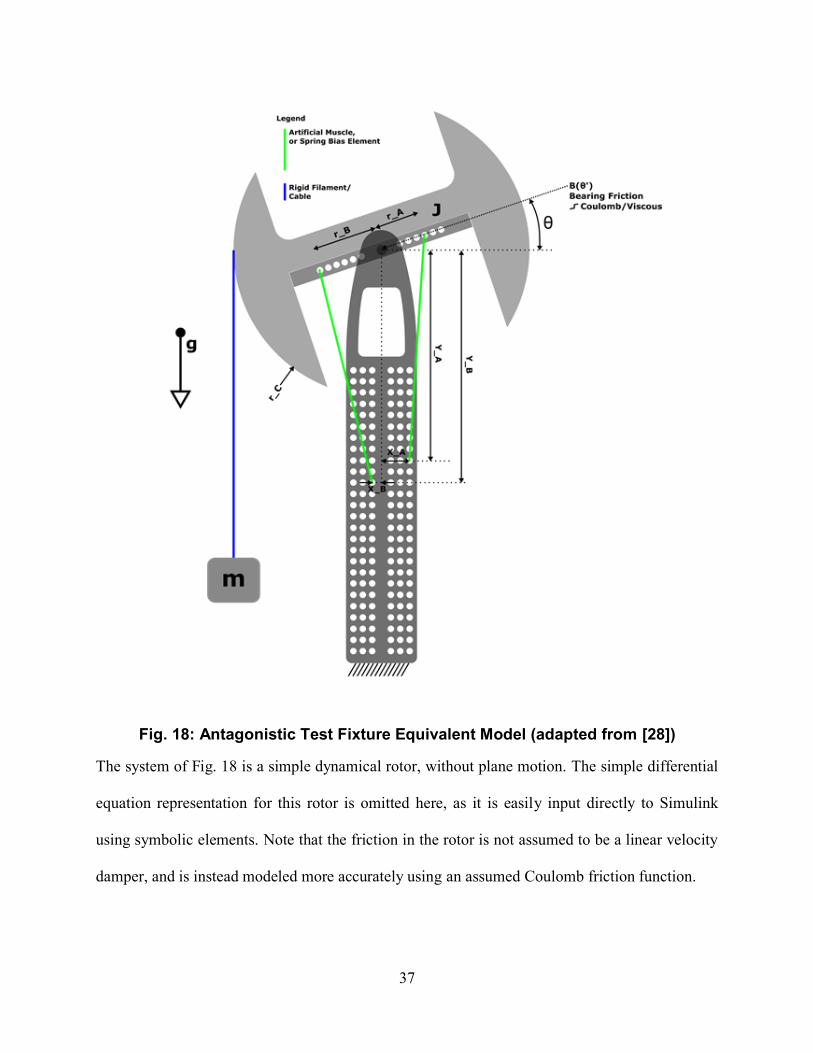
Fig. 18: Antagonistic Test Fixture Equivalent Model (adapted from [28])
The system of Fig. 18 is a simple dynamical rotor, without plane motion. The simple differential
equation representation for this rotor is omitted here, as it is easily input directly to Simulink
using symbolic elements. Note that the friction in the rotor is not assumed to be a linear velocity
damper, and is instead modeled more accurately using an assumed Coulomb friction function.

38
The complicating factors in this model are the non-linear modulated transformer functions
between the muscle/spring stimulus elements and the rotor. These elements possess length and
tension properties, which impose torque functions on the rotor. To compute these torque
functions, vector mathematics must be applied. The known vectors are:
𝐴 = �̂�𝑋𝐴 − 𝑗̂𝑌𝐴
�⃑⃑� = −�̂�𝑋𝐵 − 𝑗̂𝑌𝐵
𝑟𝐴⃑⃑⃑⃑ = �̂�𝑟𝐴 cos 𝜃 + 𝑗̂𝑟𝐴 sin 𝜃
𝑟𝐵⃑⃑ ⃑⃑ = −𝑖̂𝑟𝐵 cos 𝜃 − 𝑗̂𝑟𝐵 sin 𝜃
The vectors of interest, namely the muscle/spring elements, can now be defined in terms of
known quantities. The conclusive vectors are shown in equations (5) and (6); the vector lengths
are shown in equations (7) and (8).
𝑀𝐴⃑⃑ ⃑⃑ ⃑⃑ = 𝐴 − 𝑟𝐴⃑⃑⃑⃑
𝑀𝐵⃑⃑ ⃑⃑ ⃑⃑ = �⃑⃑� − 𝑟𝐵⃑⃑ ⃑⃑
𝑀𝐴⃑⃑ ⃑⃑ ⃑⃑ = −�̂�𝑟𝐴 cos 𝜃 − 𝑗̂𝑟𝐴 sin 𝜃 + �̂�𝑋𝐴 − 𝑗̂𝑌𝐴 (5)
𝑀𝐵⃑⃑ ⃑⃑ ⃑⃑ = 𝑖̂𝑟𝐵 cos 𝜃 + 𝑗̂𝑟𝐵 sin 𝜃 − �̂�𝑋𝐵 − 𝑗̂𝑌𝐵 (6)
𝐿𝐴 = |𝑀𝐴⃑⃑ ⃑⃑ ⃑⃑ | = √(𝑋𝐴 − 𝑟𝐴 cos 𝜃)2 + (−𝑌𝐴 − 𝑟𝐴 sin 𝜃)2 (7)
𝐿𝐵 = |𝑀𝐵⃑⃑ ⃑⃑ ⃑⃑ | = √(−𝑋𝐵 + 𝑟𝐵 cos 𝜃)2 + (−𝑌𝐵 + 𝑟𝐵 sin 𝜃)2 (8)
The length of each muscle/spring is now known in terms of the angle 𝜃 of the rotor. The torque
on the rotor due to each muscle/spring element is a function of both rotor position (the
39
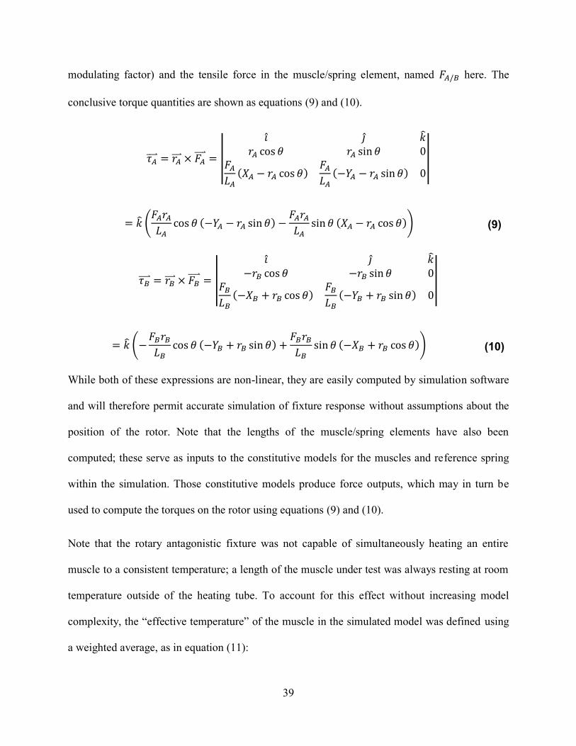
modulating factor) and the tensile force in the muscle/spring element, named 𝐹𝐴/𝐵 here. The
conclusive torque quantities are shown as equations (9) and (10).
𝜏𝐴⃑⃑ ⃑⃑ = 𝑟𝐴⃑⃑⃑⃑ × 𝐹𝐴⃑⃑⃑⃑⃑ = ||
�̂� 𝑗̂ �̂�𝑟𝐴 cos 𝜃 𝑟𝐴 sin 𝜃 0
𝐹𝐴𝐿𝐴(𝑋𝐴 − 𝑟𝐴 cos 𝜃)
𝐹𝐴𝐿𝐴(−𝑌𝐴 − 𝑟𝐴 sin 𝜃) 0
||
= �̂� (𝐹𝐴𝑟𝐴𝐿𝐴
cos 𝜃 (−𝑌𝐴 − 𝑟𝐴 sin 𝜃) −𝐹𝐴𝑟𝐴𝐿𝐴
sin 𝜃 (𝑋𝐴 − 𝑟𝐴 cos 𝜃)) (9)
𝜏𝐵⃑⃑⃑⃑⃑ = 𝑟𝐵⃑⃑ ⃑⃑ × 𝐹𝐵⃑⃑⃑⃑⃑ = ||
�̂� 𝑗̂ �̂�−𝑟𝐵 cos 𝜃 −𝑟𝐵 sin 𝜃 0
𝐹𝐵𝐿𝐵(−𝑋𝐵 + 𝑟𝐵 cos 𝜃)
𝐹𝐵𝐿𝐵(−𝑌𝐵 + 𝑟𝐵 sin 𝜃) 0
||
= �̂� (−𝐹𝐵𝑟𝐵𝐿𝐵
cos 𝜃 (−𝑌𝐵 + 𝑟𝐵 sin 𝜃) +𝐹𝐵𝑟𝐵𝐿𝐵
sin 𝜃 (−𝑋𝐵 + 𝑟𝐵 cos 𝜃)) (10)
While both of these expressions are non-linear, they are easily computed by simulation software
and will therefore permit accurate simulation of fixture response without assumptions about the
position of the rotor. Note that the lengths of the muscle/spring elements have also been
computed; these serve as inputs to the constitutive models for the muscles and reference spring
within the simulation. Those constitutive models produce force outputs, which may in turn be
used to compute the torques on the rotor using equations (9) and (10).
Note that the rotary antagonistic fixture was not capable of simultaneously heating an entire
muscle to a consistent temperature; a length of the muscle under test was always resting at room
temperature outside of the heating tube. To account for this effect without increasing model
complexity, the “effective temperature” of the muscle in the simulated model was defined using
a weighted average, as in equation (11):
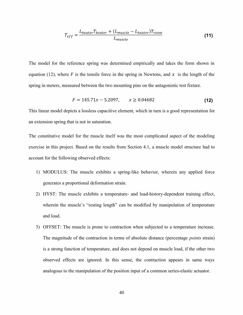
40
𝑇𝑒𝑓𝑓 =𝐿ℎ𝑒𝑎𝑡𝑒𝑟𝑇ℎ𝑒𝑎𝑡𝑒𝑟 + (𝐿𝑚𝑢𝑠𝑐𝑙𝑒 − 𝐿ℎ𝑒𝑎𝑡𝑒𝑟)𝑇𝑟𝑜𝑜𝑚
𝐿𝑚𝑢𝑠𝑐𝑙𝑒 (11)
The model for the reference spring was determined empirically and takes the form shown in
equation (12), where 𝐹 is the tensile force in the spring in Newtons, and 𝑥 is the length of the
spring in meters, measured between the two mounting pins on the antagonistic test fixture.
𝐹 = 145.71𝑥 − 5.2097, 𝑥 ≥ 0.04682 (12)
This linear model depicts a lossless capacitive element, which in turn is a good representation for
an extension spring that is not in saturation.
The constitutive model for the muscle itself was the most complicated aspect of the modeling
exercise in this project. Based on the results from Section 4.1, a muscle model structure had to
account for the following observed effects:
1) MODULUS: The muscle exhibits a spring-like behavior, wherein any applied force
generates a proportional deformation strain.
2) HYST: The muscle exhibits a temperature- and load-history-dependent training effect,
wherein the muscle’s “resting length” can be modified by manipulation of temperature
and load.
3) OFFSET: The muscle is prone to contraction when subjected to a temperature increase.
The magnitude of the contraction in terms of absolute distance (percentage points strain)
is a strong function of temperature, and does not depend on muscle load, if the other two
observed effects are ignored. In this sense, the contraction appears in same ways
analogous to the manipulation of the position input of a common series-elastic actuator.

41
The MODULUS effect is the easiest to
model; it is merely a linear spring. The
OFFSET effect is also simple to model,
because this effect appears to occur
independent of the other system effects. Thus
the OFFSET can be modeled as a true
positional offset source, with offset
magnitude a function of temperature,
positioned in series with the MODULUS
element.
The HYST effect is the most difficult to model, but it is common to use damper models for
hysteretic effects. In fact, researchers working with polymer artificial muscles coiled from
conductive thread showed that a damper model accurately described isothermal load-cycling
hysteresis within their muscles (an effect not directly investigated here) [21]. A model based on
this work provides a convenient starting point for this case. A fixed damper model in parallel
with a spring models isothermal hysteresis, but more detail must be added to account for the
muscle’s memory of its resting length. If a damper’s coefficient is negatively dependent upon
temperature, the damper will permit fast deformations at high temperatures, but resist them at
low temperatures, preventing recovery from a deformation achieved at high temperature. This is
an accurate description of the observed muscle behavior. Thus, the HYST effect is modeled
using a linear spring and damper in parallel, with the damper’s coefficient dependent upon
temperature. For simplicity, the temperature dependence of the damper element is assumed
linear.
Fig. 19: Muscle Model

42
The model as described above is illustrated in Fig. 19. Note that this model does not account for
the mass of the muscle, which is assumed to be negligible relative to the masses in the
antagonistic rotary test fixture.
From this point in the analysis, it is convenient to assess response in terms of relative strain. This
strain will be assessed with respect to a “base length”, refined as the minimum length of the
muscle before it has deformed. Strain is denoted in the simulation work associated with this
paper using the character sigma (𝜎); this notation is continued here.
𝜎 =𝐿 − 𝐿𝑏𝑎𝑠𝑒𝐿𝑏𝑎𝑠𝑒
And so:
𝐿 = 𝐿𝑏𝑎𝑠𝑒 + 𝜎𝐿𝑏𝑎𝑠𝑒
The most convenient mathematical interpretation of the muscle model will take 𝐿 or 𝜎 as an
input, and produce the resulting tensile force as an output. Certain simplifications are necessary
to accomplish this inversion. First, the springs must be modeled as tensile springs, which can
only produce tensile force, and which cannot actuate below a certain threshold force. To invert
this region of saturation, it is necessary to introduce a slight incline to the otherwise sharp cliff of
saturation. Thus, a very small strain value 𝜖 is selected, and the spring forces follow in equations
(13) and (14):
𝐹𝐾ℎ𝑦𝑠𝑡 =
{
𝐿𝑏𝑎𝑠𝑒(𝜎ℎ𝑦𝑠𝑡 − 𝜖)𝐾ℎ𝑦𝑠𝑡 + 𝐹ℎ𝑦𝑠𝑡𝑚𝑖𝑛 , 𝜎ℎ𝑦𝑠𝑡 > 𝜖
𝐹ℎ𝑦𝑠𝑡𝑚𝑖𝑛𝜖
𝜎ℎ𝑦𝑠𝑡 , 0 < 𝜎ℎ𝑦𝑠𝑡 ≤ 𝜖
0, 𝜎ℎ𝑦𝑠𝑡 ≤ 0
(13)

43
𝐹𝐾𝑚𝑜𝑑𝑢𝑙𝑢𝑠 =
{
𝐿𝑏𝑎𝑠𝑒(𝜎 − 𝜎𝑜𝑓𝑓𝑠𝑒𝑡 − 𝜎ℎ𝑦𝑠𝑡 − 𝜖)𝐾𝑚𝑜𝑑𝑢𝑙𝑢𝑠 + 𝐹𝑚𝑜𝑑𝑢𝑙𝑢𝑠𝑚𝑖𝑛 , 𝜎 − 𝜎𝑜𝑓𝑓𝑠𝑒𝑡 − 𝜎ℎ𝑦𝑠𝑡 > 𝜖
𝐹𝑚𝑜𝑑𝑢𝑙𝑢𝑠𝑚𝑖𝑛𝜖
(𝜎 − 𝜎𝑜𝑓𝑓𝑠𝑒𝑡 − 𝜎ℎ𝑦𝑠𝑡), 0 < (𝜎 − 𝜎𝑜𝑓𝑓𝑠𝑒𝑡 − 𝜎ℎ𝑦𝑠𝑡) ≤ 𝜖
0, (𝜎 − 𝜎𝑜𝑓𝑓𝑠𝑒𝑡 − 𝜎ℎ𝑦𝑠𝑡) ≤ 0
(14)
In equations (13) and (14), the expressions 𝐹ℎ𝑦𝑠𝑡𝑚𝑖𝑛 and 𝐹𝑚𝑜𝑑𝑢𝑙𝑢𝑠𝑚𝑖𝑛 are the minimum forces
required to begin deforming the respective springs. The expression for damping is simple:
𝐹𝐵ℎ𝑦𝑠𝑡 = 𝐵ℎ𝑦𝑠𝑡𝐿𝑏𝑎𝑠𝑒𝜎ℎ𝑦𝑠𝑡̇
The sum of the forces is computed as follows, and yields a final differential equation
representation in equation (15).
𝐹𝐵ℎ𝑦𝑠𝑡 + 𝐹𝐾ℎ𝑦𝑠𝑡 − 𝐹𝐾𝑚𝑜𝑑𝑢𝑙𝑢𝑠 = 0
𝐵ℎ𝑦𝑠𝑡𝐿𝑏𝑎𝑠𝑒𝜎ℎ𝑦𝑠𝑡̇ = 𝐹𝐾𝑚𝑜𝑑𝑢𝑙𝑢𝑠 − 𝐹𝐾ℎ𝑦𝑠𝑡
𝜎ℎ𝑦𝑠𝑡̇ =𝐹𝐾𝑚𝑜𝑑𝑢𝑙𝑢𝑠 − 𝐹𝐾ℎ𝑦𝑠𝑡
𝐵ℎ𝑦𝑠𝑡𝐿𝑏𝑎𝑠𝑒 (15)
The value of 𝜎𝑜𝑓𝑓𝑠𝑒𝑡 must be defined. The results from Section 4.1 showed that the offset
element obeys a temperature law, which has been measured empirically. A quadratic relation
appeared to provide a suitable temperature law, so the offset function is defined accordingly in
equation (16):
𝜎𝑜𝑓𝑓𝑠𝑒𝑡 = 𝐴𝑇2 + 𝐵𝑇 + 𝐶 (16)
Note that, for consistency with the rest of the model, the value of 𝜎𝑜𝑓𝑓𝑠𝑒𝑡 was defined to have
units of pure fractional strain, not percentage points. This is a departure from the notation used
in Fig. 15 and related tests.

44
Finally, the relation between temperature and the coefficient of the HYST damping element must
be defined. A linear relation is selected for simplicity, as shown in equation (17):
𝐵ℎ𝑦𝑠𝑡 = 𝐻𝐵ℎ𝑦𝑠𝑡 (𝑇 + 𝑇ℎ𝑦𝑠𝑡𝑜𝑓𝑓𝑠𝑒𝑡) (17)
All of the models documented here were simple enough to ingress into the MATLAB/Simulink
environment. The Simulink model subsystem for the muscle itself is shown in Fig. 20. The
complete subsystem for the fixture, configured with a single muscle, is shown in Fig. 21. Finally,
the test configuration for the entire system (set up for the sawtooth test stimulus) is shown in Fig.
22.
Fig. 20: Simulink Muscle Subsystem

45
Fig. 21: Simulink Joint Subsystem w/ One Muscle
Fig. 22: Complete Simulink Model w/ Experimental Stimulus
4.3 PARAMETER ESTIMATION FINDINGS
Before the parameters of the muscle could be determined, it was necessary to find the values of
the rotor rotational inertia and damping. This was accomplished using the Simulink Parameter
Estimation utility, over the five reference spring oscillation sample sets collected before muscle
testing. Two separate parameter estimations were performed, one using the more accurate
Coulomb damping model, and another using the less accurate but simpler linear damping model.

46
Table 1 shows the results of the reference spring parameter matching exercise.
Table 1: Reference Spring Oscillation Parameter Matching Results
Test Configuration Parameter Value
Coulomb Damping Inertia J 0.00124103 kg − m2
Damping D 0.00545940 N −m
Linear Damping Inertia J 0.00131390 kg − m2
Damping D 0.00415667 N −m
The reference spring parameter matching exercise was trivial due to the small number of
parameters under investigation. The muscle parameter matching exercise was much more
computationally intensive and therefore slower. The parameters under analysis were
[𝐹ℎ𝑦𝑠𝑡𝑚𝑖𝑛 , 𝐾ℎ𝑦𝑠𝑡, 𝐹𝑚𝑜𝑑𝑢𝑙𝑢𝑠𝑚𝑖𝑛 , 𝐾𝑚𝑜𝑑𝑢𝑙𝑢𝑠, 𝐻𝐵ℎ𝑦𝑠𝑡 , 𝑇ℎ𝑦𝑠𝑡𝑜𝑓𝑓𝑠𝑒𝑡 , 𝐴, 𝐵, 𝐶]. The 𝐹𝑚𝑜𝑑𝑢𝑙𝑢𝑠𝑚𝑖𝑛 and
𝐾𝑚𝑜𝑑𝑢𝑙𝑢𝑠 parameters could be easily estimated based on the initial resting state of the system, but
the remaining parameters had to be estimated computationally. Three staircase stimulus datasets
with different load weights were selected as the estimation experiments; the data from these tests
were imported into Simulink and a nonlinear parameter estimation exercise was executed (note
that the Coulomb damping model was used for the fixture model in this step). The results of the
estimation exercise are shown in Table 2.
Table 2: Muscle Model Parameter Estimation Results
Parameter Name Value Estimation Technique
𝐴 −1.17832e − 05 1/K2 Computational Search
𝐵 1.40992e − 05 1/K Computational Search
𝐶 0.00881695 Computational Search
𝐹ℎ𝑦𝑠𝑡𝑚𝑖𝑛 1.75489 N Computational Search
𝐾ℎ𝑦𝑠𝑡 415.189N
m
Computational Search
𝐹𝑚𝑜𝑑𝑢𝑙𝑢𝑠𝑚𝑖𝑛 3.789 N Manual Estimation
𝐾𝑚𝑜𝑑𝑢𝑙𝑢𝑠 186N
m
Manual Estimation
𝐻𝐵ℎ𝑦𝑠𝑡 −545.907 N − s
m − K
Computational Search

47
𝑇ℎ𝑦𝑠𝑡𝑜𝑓𝑓𝑠𝑒𝑡 −243.380 ℃ Computational Search
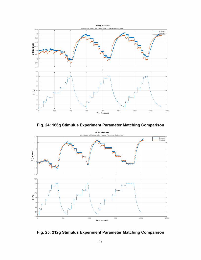
The estimation response curves are shown alongside the experimental data curves in Fig. 23, Fig.
24 and Fig. 25. Note that all the data in these three figures were used as reference data in the
parameter estimation exercise.
Fig. 23: 139g Stimulus Experiment Parameter Matching Comparison
48
Fig. 24: 166g Stimulus Experiment Parameter Matching Comparison
Fig. 25: 212g Stimulus Experiment Parameter Matching Comparison

49
Because all the staircase datasets were used in parameter estimation, the sawtooth dataset was
selected as a downstream verification dataset. The output of the simulated system, when
stimulated using the temperature curve from the sawtooth experiment, is shown in Fig. 26.
Fig. 26: Downstream Verification Comparison of Measured and Simulated Response Datasets for Sawtooth Stimulus Experiment
Note that the downstream verification plot closely follows the general trend of the experimental
plot. The saturation condition (in which the coils of the muscle fiber press up against one
another) was not modeled in the simulated muscle element, and the resulting error in response
can be observed in the first two peaks of Fig. 26. Simulation noise can also be observed in the
first two relaxations of Fig. 26; this noise was caused by overshoot inside the spring saturation
regions of the muscle model. If these two phenomena are ignored, the simulated response
appears to be an accurate reproduction of the real-world system output.
To confirm the above assumptions about the origins of error in Fig. 26, the muscle model and
simulation configuration were augmented using small changes designed to address hypothetical
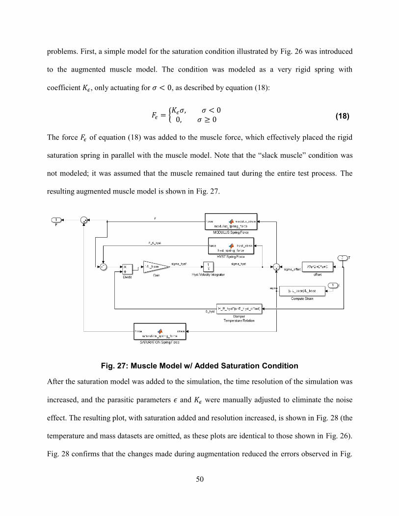
50
problems. First, a simple model for the saturation condition illustrated by Fig. 26 was introduced
to the augmented muscle model. The condition was modeled as a very rigid spring with
coefficient 𝐾𝜖, only actuating for 𝜎 < 0, as described by equation (18):
𝐹𝜖 = {𝐾𝜖𝜎, 𝜎 < 00, 𝜎 ≥ 0
(18)
The force 𝐹𝜖 of equation (18) was added to the muscle force, which effectively placed the rigid
saturation spring in parallel with the muscle model. Note that the “slack muscle” condition was
not modeled; it was assumed that the muscle remained taut during the entire test process. The
resulting augmented muscle model is shown in Fig. 27.
Fig. 27: Muscle Model w/ Added Saturation Condition
After the saturation model was added to the simulation, the time resolution of the simulation was
increased, and the parasitic parameters 𝜖 and 𝐾𝜖 were manually adjusted to eliminate the noise
effect. The resulting plot, with saturation added and resolution increased, is shown in Fig. 28 (the
temperature and mass datasets are omitted, as these plots are identical to those shown in Fig. 26).
Fig. 28 confirms that the changes made during augmentation reduced the errors observed in Fig.
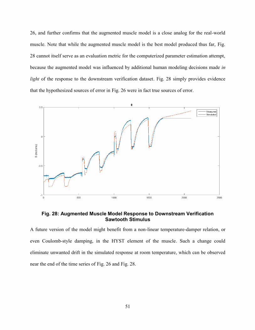
51
26, and further confirms that the augmented muscle model is a close analog for the real-world
muscle. Note that while the augmented muscle model is the best model produced thus far, Fig.
28 cannot itself serve as an evaluation metric for the computerized parameter estimation attempt,
because the augmented model was influenced by additional human modeling decisions made in
light of the response to the downstream verification dataset. Fig. 28 simply provides evidence
that the hypothesized sources of error in Fig. 26 were in fact true sources of error.
Fig. 28: Augmented Muscle Model Response to Downstream Verification Sawtooth Stimulus
A future version of the model might benefit from a non-linear temperature-damper relation, or
even Coulomb-style damping, in the HYST element of the muscle. Such a change could
eliminate unwanted drift in the simulated response at room temperature, which can be observed
near the end of the time series of Fig. 26 and Fig. 28.

52
4.4 CONTROLS FINDINGS
The ultimate goal of this project was to develop an environment for investigating controls for
polymer artificial muscles, and to demonstrate a potential controls model. For simplicity, PI
(proportional-integral) control was selected as the controller type. Simulink conveniently
includes a discrete PI controller block, so the test simulation environment was set up around that
controller block.
For the in-silico controls test, the simulated joint model was updated to include two
antagonistically coupled muscle models, as shown in Fig. 29.
Fig. 29: Antagonistic Simulation Arrangement
Note that this antagonistic model used the simpler, linear model for damping, instead of the non-
linear Coulomb model. The antagonistic model also included the augmented version of the
muscle model, described in Section 4.3.
Heating was simulated using a linear energy flow model, and cooling was simulated according to
Newton’s cooling law. The rate coefficients for each of these models were empirically measured
using a real heater tube, so the simulated heating and cooling rates would match real-world
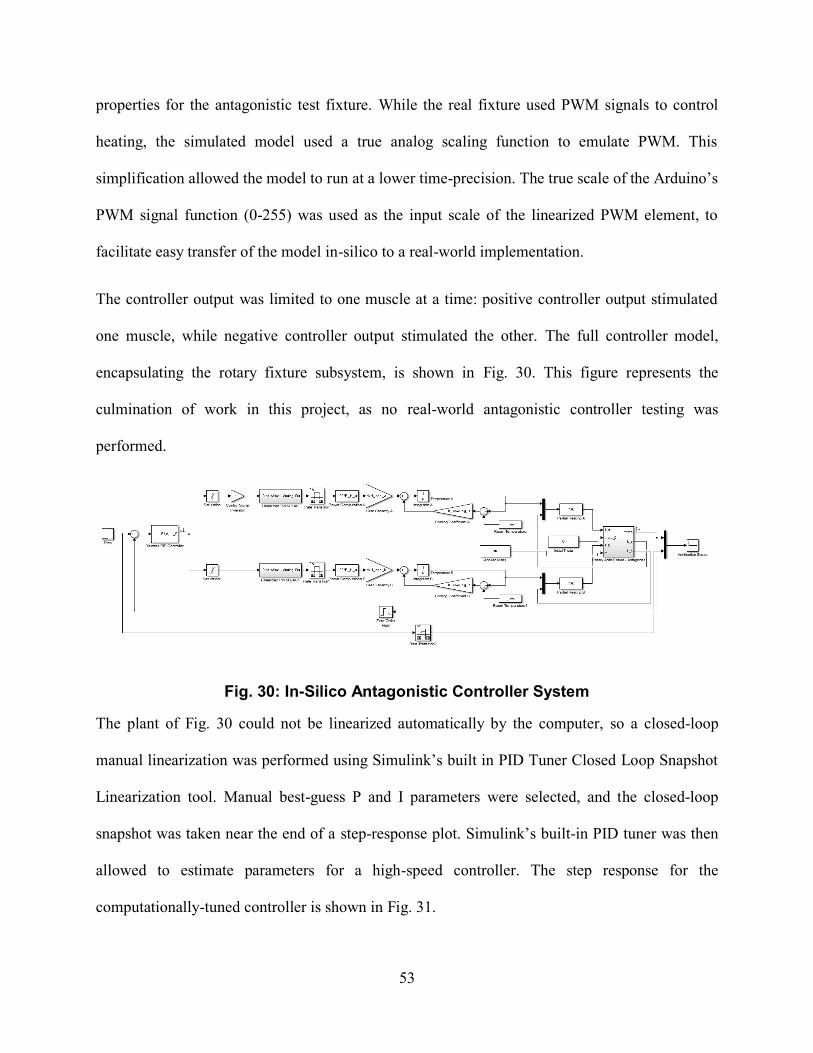
53
properties for the antagonistic test fixture. While the real fixture used PWM signals to control
heating, the simulated model used a true analog scaling function to emulate PWM. This
simplification allowed the model to run at a lower time-precision. The true scale of the Arduino’s
PWM signal function (0-255) was used as the input scale of the linearized PWM element, to
facilitate easy transfer of the model in-silico to a real-world implementation.
The controller output was limited to one muscle at a time: positive controller output stimulated
one muscle, while negative controller output stimulated the other. The full controller model,
encapsulating the rotary fixture subsystem, is shown in Fig. 30. This figure represents the
culmination of work in this project, as no real-world antagonistic controller testing was
performed.
Fig. 30: In-Silico Antagonistic Controller System
The plant of Fig. 30 could not be linearized automatically by the computer, so a closed-loop
manual linearization was performed using Simulink’s built in PID Tuner Closed Loop Snapshot
Linearization tool. Manual best-guess P and I parameters were selected, and the closed-loop
snapshot was taken near the end of a step-response plot. Simulink’s built-in PID tuner was then
allowed to estimate parameters for a high-speed controller. The step response for the
computationally-tuned controller is shown in Fig. 31.

54
Fig. 31: PI Controller Step Response
The effect of “re-training” in the HYST element of the muscle model provoked concern about
the PI controller’s ability to maintain zero steady-state error during repeated cycling events and
non-constant loads. To test the validity of this concern, various test stimuli were applied to the
in-silico model.
First, a symmetric pulsed input was applied. The response is shown in Fig. 32.
Fig. 32: PI Controller Square Response

55
Next, a step input was applied, and a mass stimulus was applied instantaneously, after a delay
period. The response is shown in Fig. 33. This outcome serves to illustrate the rotary system’s
ability to compensate for changes in applied load.
Fig. 33: PI Controller Mass Step Response
Next, during a normal step response, the mass stimulus was fluctuated using sine wave functions
of increasing frequencies. The resulting response curves are shown in Fig. 34, Fig. 35 and Fig.
36. Note that the system is highly sensitive to external load stimulus, because of the intrinsic
pliability present in the MODULUS element of the muscle model.
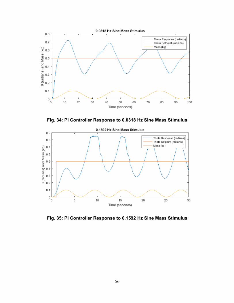
56
Fig. 34: PI Controller Response to 0.0318 Hz Sine Mass Stimulus
Fig. 35: PI Controller Response to 0.1592 Hz Sine Mass Stimulus
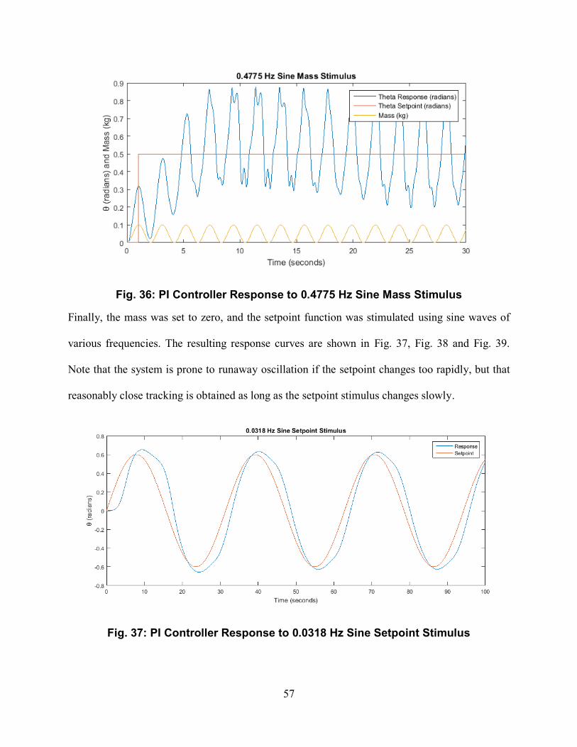
57
Fig. 36: PI Controller Response to 0.4775 Hz Sine Mass Stimulus
Finally, the mass was set to zero, and the setpoint function was stimulated using sine waves of
various frequencies. The resulting response curves are shown in Fig. 37, Fig. 38 and Fig. 39.
Note that the system is prone to runaway oscillation if the setpoint changes too rapidly, but that
reasonably close tracking is obtained as long as the setpoint stimulus changes slowly.
Fig. 37: PI Controller Response to 0.0318 Hz Sine Setpoint Stimulus
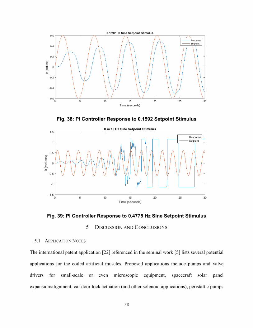
58
Fig. 38: PI Controller Response to 0.1592 Setpoint Stimulus
Fig. 39: PI Controller Response to 0.4775 Hz Sine Setpoint Stimulus
5 DISCUSSION AND CONCLUSIONS
5.1 APPLICATION NOTES
The international patent application [22] referenced in the seminal work [5] lists several potential
applications for the coiled artificial muscles. Proposed applications include pumps and valve
drivers for small-scale or even microscopic equipment, spacecraft solar panel
expansion/alignment, car door lock actuation (and other solenoid applications), peristaltic pumps

59
using sequentially actuated fiber segments, optical device actuators, haptic feedback devices,
porosity control, and various other applications. This section treats a few of those proposed
applications in context of the controls findings from the project.
In brief, this project found that twisted polymer artificial muscles could actuate repeatably under
constant loads, but changed operating region (“resting length”) when subjected to varying loads
during operation. This outcome suggests that applications for the muscles fall into two broad
categories: those that impart unpredictably varying tension on the fiber element, and those that
produce repeatable or constant loading profiles. Instances that require constant loading profiles
are immediate candidates for application of the muscle technology discussed herein, as the
muscles become very easy to model when they do not undergo a change in resting length.
Examples include some valves and pumps, solenoid applications, optical device actuators, and
purely visual event controllers (e.g. facial features on a humanoid robot).
Use cases in which the load profile range is unpredictable, or simply very wide, may still be
candidates for application of twisted polymer muscle technology, but these applications will
require more careful control and may exhibit range-of-motion limitations. Examples of more
challenging applications include haptic feedback, complex manifold control and pumping,
reversible spacecraft solar panel or solar sail expansion, and pure robotics actuation (e.g.
humanoid joint movement). Recent work by Yip and Niemeyer [21] showed that twisted
polymer muscles spun from whole conductive threads (rather than monofilaments) made suitable
actuators for a robotic hand. That research did not investigate or report on in-situ training effects,
which could impact grasping strength or limit muscle range of motion, but the success of a
relatively complex application bodes well for this technology.

60
Note that the applications for twisted polymer muscles are not identical to those applications
previously documented for traditional muscle analogs, though there is some overlap. The
polymer muscles are especially flexible, and very weight-efficient, so they are well suited to
space applications. Because of their low power efficiency, they are poorly suited for traditional
power robotics applications such as dynamic manipulation. Nevertheless, as shown in this
project, these artificial muscles may still find applications in power robotics. Consider a robotic
linkage containing clutches, brakes or dampers at its joints. This kind of element is common if an
armature will be subjected to unknown forces, or simply needs to be back drivable. Twisted
polymer muscles may satisfactorily control the dynamical parameters in those kinds of auxiliary
drive elements, while more traditional actuators execute primary actuation maneuvers.
5.2 FURTHER RESEARCH
Targets for future research include more precise thermal characterizations of muscle properties,
better mathematical modeling, mitigation methods for the “retraining” effect, and faster cooling.
Specifically, future projects should investigate surface-layer or intrinsic heating elements, rather
than using large external heater tubes with unnecessarily high heat capacities. Haines et al. [5]
and Mirvakili et al. [25] have already shown that silver coatings or paints can be used as surface-
layer heating elements. Yip and Niemeyer [21] have demonstrated that this method of heating
still works when muscles are coiled from whole threads (rather than monofilaments). At a
minimum, it is recommended that future experimenters attempt to obtain pre-plated precursor
fibers or the proper SPI Flash-Dry paint compound, in order to reproduce the heating elements
from [5] and/or [25].
61
The major challenge for surface-layer heating is cost, as silver is typically the conductive agent.
A safe, flexible, low cost alternative surface heating agent would be useful to drive down the cost
of high-speed muscles. This is a potential area for future research.
The issue of re-training during loading at temperature remains a controls challenge, though many
applications can avoid this problem by imparting predictable loads on the muscle. Yip and
Niemeyer [21] did not report the re-training effect, but their muscles were constructed from
thread precursors, and treated during “initial training” at a higher peak temperature. It is possible
that one of these changes in precursor or process reduced the muscles’ propensity for complex
hysteretic behavior ([21] reports a fairly straightforward hysteresis loop effect during isothermal
load variation). Further investigation or coordination with those researchers may reveal useful
information.
The geometric means by which the polymer muscles achieve actuation should be transferrable to
other materials with similar molecular structures. Further research into the materials background
for the effects documented herein could reveal a precursor material that yields higher efficiency,
or reduces the re-training effect.
In a push toward testing efficiency, future projects should work to develop more precise, more
automated, non-inertial test fixtures, in which applied force functions are generated using a
control system and not using a hanging weight or spring. This development effort could be
avoided by the acquisition of a thermomechanical analysis machine, but there will always be
some advantages to developing custom test fixtures with the target application in mind.

62
5.3 PROJECT CONCLUSION
The research performed in this project demonstrated that the twisted polymer artificial muscles
of Haines et al. [5] contain useful features, but are also subject to certain mechanical limitations
associated with model complexity. While other researchers have characterized the initial training
of the muscle, no known published work has documented the property of re-training during load
changes at high temperature. This project produced empirical evidence for that effect, and further
documented a simple model with predictive power over the artificial muscle fibers.
The robotic design portion of this project was simple, but it provided the author with an
opportunity to develop a research tool that functioned like a potential application device, namely
the antagonistic muscle fixture. While the fixture was never configured or operated in the full
antagonistic configuration, it was used to collect empirical data that drove in-silico testing, and it
could be easily re-used by a future researcher for similar testing. Design challenges in this
project included test device integration, low-impact mechanical measurement, and unknown
operating parameters of the muscle. The fixture’s construction is extremely strong; it was
designed to accommodate several muscles acting in parallel under high tension. Finite element
analyses for critical parts, while omitted from this report for brevity, are included in the reference
package design files.
In conclusion, the author wishes to thank the countless supporting parties to this work, and to
reiterate that the technology treated herein holds promise for application in the field of soft
robotics, and in a broad range of other technical fields. Twisted polymer artificial muscles are
not without their limitations, but this low-cost, lightweight alternative to more traditional
electromechanical actuators indicates an early step in the right direction for soft robotics
actuation.

63
6 REFERENCES
[1] “agonist muscle.” Taber’s Medical Dictionary. 2015. Retrieved from http://www.tabers.com/tabersonline/view/Tabers-
Dictionary/765961/all/muscle
[2] C. Chou, B. Hannaford, Measurement and Modeliing of McKibben Pneumatic Artificial Muscles. IEEE Trans. Robot.
Auto. 12 (1) 90-102 (1996).
[3] C. L. Choy, F. C. Chen, K. Young, Negative Thermal Expansion in Oriented Crystalline Polymers. Jour. Poly. Sci.
Poly. Phys. Ed. 19 (2), 335-352 (1981).
[4] C. S. Haines et al., Supplementary Materials for Artificial Muscles from Fishing Line and Sewing Thread. Science 343,
868 (2014). Supplementary Materials from Science online.
[5] C.S. Haines et al., Artificial muscles from fishing line and sewing thread. Science 343, 868-872 (2014).
[6] C.S. Haines, How to Make an Artificial Muscle Out of Fishing Line (Science Friday, New York, 2014). Retrieved from http://www.sciencefriday.com/blogs/03/06/2014/how-to-make-an-artificial-muscle-out-of-fishing-line.html
[7] DARPA, Upgraded Atlas robot to go wireless as the stakes are raised for the DARPA Robotics Challenge finals
(DARPA, Arlington, 2015). Retrieved from http://www.darpa.mil/NewsEvents/Releases/2015/01/20.aspx
[8] Dynalloy, 70°C and 90°C Flexinol® Actuator Wire Price Guide (Dynalloy, Inc., Irvine, 2014). Retrieved from http://www.dynalloy.com/flexwire_70_90.php
[9] Dynalloy, Technical Characteristics of Flexinol® Actuator Wire (Dynalloy, Inc., Irvine, 2014). Retrieved from
http://www.dynalloy.com/pdfs/TCF1140.pdf
[10] F. Daerden, D. Lefeber, B. Verrelst, R. Van Ham, Pleated pneumatic artificial muscles: actuators for automation and robotics. Proc. 2011 IEEE/ASME Conf. Adv. Intelligent Mechatronics, Como, Italy (2001).
[11] H. Herr, R. Kornbluh., New horizons for orthotic and prosthetic technology: artificial muscle for ambulation. Proc.
SPIE 5385, Smart Structures and Materials 2004: Electroactive Polymer Actuators and Devices (2004).
[12] H. Koerner, G. Price, N. A. Pearce, M. Alexander, R. A. Vaia, Remotely actuated polymer nanocomposites–stress-recovery of carbon-nanotube-filled thermoplastic elastomers. Nat. Mat. 3 115-120 (2004).
[13] J. Cui et al., Combinatorial search of thermoelastic shape-memory alloys with extremely small hysteresis width. Nat.
Mat. 5 286-290 (2006).
[14] J. D. W. Madden et al., Artificial muscle technology: physical principles and naval prospects. IEEE Jour. Ocean. Eng. 29 (3) 706-728 (2004).
[15] J. Foroughi et al. Torsional carbon nanotube artificial muscles. Science 334 494-497 (2011).
[16] J. L. Serres, thesis, Wright State University (2008).
[17] J. Leng, X. Lan, Y. Liu, S. Du, Shape-memory polymers and their composites: stimulus methods and applications. Prog. Mat. Sci. 56 1077-1135 (2011).
[18] J. Yamaguchi, D. Nishino, A. Takanishi, Realization of dynamic biped walking varying joint stiffness using
antagonistic driven joints. Proc. 1998 IEEE Conf. Rob. Auto., Leuven, Belgium (1998).
[19] K. Hosoda, T. Takuma, A. Nakamoto, S. Hayashi, Biped robot design powered by antagonistic pneumatic actuators for multi-model locomotion. Robotics and Autonomous Systems 56, 46-53 (2008).
[20] M. D. Lima et al. Electrically, chemically, and photonically powered torsional and tensile actuation of hybrid carbon
nanotube yarn muscles. Science 338 928-932 (2012).
[21] M.C. Yip, G. Niemeyer, High-Performance Robotic Muscles from Conductive Nylon Sewing Thread. Proc. 2015 IEEE Conf. Rob. Auto., Seattle, Washington (2015).
[22] N. Li, C.S. Haines, M.D. Lima, M.J. de Andrade, S. Fang, J. Oh, M.E. Kozlov, F. Goktepe, O. Oktepe, D. Suh, R.H.
Baughman, “Coiled and non-coiled twisted nanofiber yarn and polymer fiber torsional and tensile actuators,”
International Patent Application PCT/US2013/053227, Feb 6, 2014
[23] R. J. Maring, “Potentiometer mounting,” U.S. Patent 2937861, May 24, 1960.
[24] R. Pelrine, R. Kornbluh, Q. Pei, J. Joseph, High-speed electrically actuated elastomers with strain greater than 100%.
Science 287 836-839 (2000).

64
[25] S. M. Mirvakili et al., Simple and strong: twisted silver painted nylon artificial muscle actuated by Joule heating. Proc.
SPIE 9056, Electroactive Polymer Actuatots and Devices (2014).
[26] Shadow Robot Company, Air Muscle Hand (Shadow Robot Company, London). Image provided by owner and used by
express permission.
[27] Shadow Robot Company, Shadow Dexterous Hand Technical Specification (Shadow Robot Company, London, 2013).
Retrieved from http://www.shadowrobot.com/wp-content/uploads/shadow_dexterous_hand_technical_specification_E1_20130101.pdf
[28] T. Chaulk, W. D. Hunt, J. Johnson, Dynamic Model of an Artificial Muscle Test Fixture. 2016, C-Term ME/RBE 4322,
Worcester Polytechnic Institute. [Unpublished College Coursework].
[29] Y. Bar-Cohen, Electroactive Polymer (EAP) Actuators as Artificial Muscles – Reality, Potential, and Challenges (SPIE, Bellingham, ed. 2, 2004).
[30] Y. Kobayashi, A. Keller, The temperature coefficient of the c lattice parameter of polyethylene; an example of thermal
shrinkage along the chain direction. Polymer 11 (2), 114-117 (1970).

65
APPENDIX A ANTAGONISTIC STIMULUS FIXTURE DESIGN DOCUMENTS
The following pages contain mechanical specification drawings for the antagonistic figure. These
drawings provide reference and replication information for the fixture provided to the Soft Robotics
Laboratory at WPI.

66
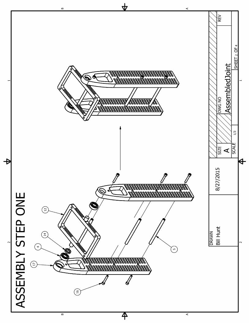
67

68

69

70

71

72

73

74

75
76
APPENDIX B ANTAGONISTIC STIMULUS FIXTURE SOFTWARE
This appendix lists the primary source code files necessary for the operation of the antagonistic test
fixture. Note that additional simple scripts were also created, using the same libraries, to facilitate tests
without temperature stimuli, and calibration runs. An older, single channel version of the antagonistic
test script was also used for tubular heater control. These ancillary scripts are omitted from this report
for brevity, but all test scripts from this project are in custody of the WPI Soft Robotics Laboratory, c/o
Prof. Cagdas Onal. As noted previously, this project did not use any source control repository or formal
versioning, because the number of software tools developed was so small.
Source and license information is provided for each program, under its header. All *.ino programs are
intended to execute on the Arduino Duemilanove or Uno board, and all *.py programs and modules are
designed to execute under Python 2.7.10 32-bit.
License Text – MIT License (See notes about granular application) NOTE: THIS LICENSE NOTICE APPLIES GRANULARLY TO THE FILES
arduino.py
prototype/prototype.ino
AND NOT TO ANY OTHER FILES IN THIS MQP, INCLUDING THE PROJECT REPORT IN WHICH COPIES OF THE LICENSED
FILES HAVE BEEN EMBEDDED
Copyright (c) 2009-2010 Akash Manohar J <[email protected]>
Permission is hereby granted, free of charge, to any person obtaining a copy
of this software and associated documentation files (the "Software"), to deal
in the Software without restriction, including without limitation the rights
to use, copy, modify, merge, publish, distribute, sublicense, and/or sell
copies of the Software, and to permit persons to whom the Software is
furnished to do so, subject to the following conditions:
The above copyright notice and this permission notice shall be included in
all copies or substantial portions of the Software.
THE SOFTWARE IS PROVIDED "AS IS", WITHOUT WARRANTY OF ANY KIND, EXPRESS OR
IMPLIED, INCLUDING BUT NOT LIMITED TO THE WARRANTIES OF MERCHANTABILITY,
FITNESS FOR A PARTICULAR PURPOSE AND NONINFRINGEMENT. IN NO EVENT SHALL THE
AUTHORS OR COPYRIGHT HOLDERS BE LIABLE FOR ANY CLAIM, DAMAGES OR OTHER
LIABILITY, WHETHER IN AN ACTION OF CONTRACT, TORT OR OTHERWISE, ARISING FROM,
OUT OF OR IN CONNECTION WITH THE SOFTWARE OR THE USE OR OTHER DEALINGS IN
THE SOFTWARE.
Arduino Interface Program – prototype/prototype.ino #ifndef SERIAL_RATE
#define SERIAL_RATE 115200
#endif
#ifndef SERIAL_TIMEOUT
#define SERIAL_TIMEOUT 5

77
#endif
void setup() {
Serial.begin(SERIAL_RATE);
Serial.setTimeout(SERIAL_TIMEOUT);
}
void loop() {
int pin = 0;
switch (readData()) {
case 0 :
//set digital low
//set digital high
pin = readData();
pinMode(pin, OUTPUT);
digitalWrite(pin, LOW); break;
case 1 :
//set digital high
pin = readData();
pinMode(pin, OUTPUT);
digitalWrite(pin, HIGH); break;
case 2 :
//get digital value
Serial.println(digitalRead(readData())); break;
case 3 :
// set analog value
pin = readData();
pinMode(pin, OUTPUT);
analogWrite(pin, readData()); break;
case 4 :
//read analog value
Serial.println(analogRead(readData())); break;
case 99:
//just dummy to cancel the current read, needed to prevent lock
//when the PC side dropped the "w" that we sent
break;
}
}
char readData() {
Serial.println("w");
while(1) {
if(Serial.available() > 0) {
return Serial.parseInt();
}
}
}
Arduino Prototyping Interface Script – arduino.py #!/usr/bin/env python
# -*- coding: utf-8 -*-
import serial
import time
class Arduino(object):
def __init__(self, port, baudrate=115200):
self.serial = serial.Serial(port, baudrate, timeout=1)
self.serial.write(b'99')
def __str__(self):
return "Arduino is on port %s at %d baudrate" %(self.serial.port, self.serial.baudrate)
def setLow(self, pin):
self.__sendData('0')
self.__sendData(pin)
return True

78
def setHigh(self, pin):
self.__sendData('1')
self.__sendData(pin)
return True
def getState(self, pin):
self.__sendData('2')
self.__sendData(pin)
return self.__formatPinState(self.__getData()[0])
def analogWrite(self, pin, value):
self.__sendData('3')
self.__sendData(pin)
self.__sendData(int(value))
return True
def analogRead(self, pin):
self.__sendData('4')
self.__sendData(pin)
return self.__getData()
def __sendData(self, serial_data):
while(self.__getData()[0] != "w"):
pass
serial_data = str(serial_data).encode('utf-8')
self.serial.write(serial_data)
def __getData(self):
input_string = self.serial.readline()
if input_string is None:
return "\n"
else:
input_string = input_string.decode('utf-8')
return input_string.rstrip('\n')
def __formatPinState(self, pinValue):
if pinValue == '1':
return True
else:
return False
def close(self):
self.serial.close()
return True
AMPROBE TMD-56 Interface Module Script – amprobe.py (See notes about granular license
application) # This source is based on code from the artisan-roaster-scope project at https://github.com/artisan-
roaster-scope/artisan
# The artisan-roaster-scope project is licensed under GPL v3. To comply with the terms of that license,
GPL v3 applies granularly
# to this file. Note that the GPL v3 does not apply to the other files in the Polymer Muscle MQP
project, INCLUDING THE PROJECT REPORT IN WHICH COPIES OF THE LICENSED FILES HAVE BEEN EMBEDDED, unless
otherwise specified.
# This program provides an interface to the Amprobe TMD-56 thermocouple meter T1 and T2 in Python
# REQUIREMENTS
# python
# pyserial
import serial
import time
import binascii
from threading import Thread, Lock
class AmprobeMeter:
79
__stableT1 = 0
__stableT2 = 0
port = ''
__thread = None
__lock = None
def __init__(self, port):
self.port = port
self.__lock = Lock()
self.__thread = Thread(target=self.__readMeter)
self.__thread.daemon = 1
self.__thread.start()
def getTemperatures(self):
with self.__lock:
return self.__stableT1, self.__stableT2
def __readMeter(self):
while(self.__thread.isAlive()):
try:
ser = serial.Serial(self.port, baudrate=19200, bytesize=8, parity='E', stopbits=1,
timeout=1)
command = "#0A0000NA2\r\n"
ser.write(command)
r = ser.read(14)
ser.close()
#convert to binary to hex string
s1 = binascii.hexlify(r[5] + r[6])
s2 = binascii.hexlify(r[10]+ r[11])
#we convert the strings to integers. Divide by 10.0 (decimal position)
t1 = int(s1,16)/10.
t2 = int(s2,16)/10.
with self.__lock:
self.__stableT1 = t1
self.__stableT2 = t2
except serial.SerialException, e:
print e
Temperature Control, Test and Logging Script – tempTest.py import amprobe
import time
import datetime
import arduino
from threading import Thread, Lock
class TempController:
__arduinoA = None
__arduinoB = None
__meter = None
__pinA = 0
__pinB = 0
__thread = None
__outputThread = None
__prevUpdateTime = 0
__period = 0
__mainThreadLock = None
__outputThreadLock = None
__enabled = 0
__currentOutputA = 0
__currentOutputB = 0
__setpointA = 0
__setpointB = 0
__kC = 0
__kF = 0
__kP = 0

80
__kI = 0
__ILimit = 0
__accumulatorA = 0
__accumulatorB = 0
__prevUnstableTimeA = 0
__prevUnstableTimeB = 0
__tempStableA = 0
__tempStableB = 0
__controlScale = 0.55
__temperatureUpdate = 0
__currentTemperatureA = 0
__currentTemperatureB = 0
__prevTemperatureA = 0
__prevTemperatureB = 0
__temperatureSteadyTime = 10
__tempThresh = 1.0
def __init__(self, arduinoAPort, arduinoBPort, amprobePort, temperaturePinA, temperaturePinB,
updatePeriod,\
kC, kF, kP, kI, accumLimit, logFileName):
self.__arduinoA = arduino.Arduino(arduinoAPort)
self.__arduinoB = arduino.Arduino(arduinoBPort)
time.sleep(1)
self.__meter = amprobe.AmprobeMeter(amprobePort)
self.__pinA = temperaturePinA
self.__pinB = temperaturePinB
self.__period = updatePeriod
self.__prevUpdateTimeA = time.time()
self.__prevUpdateTimeB = self.__prevUpdateTimeA
self.__prevUnstableTimeA = self.__prevUpdateTimeA
self.__prevUnstableTimeB = self.__prevUpdateTimeB
self.__kC = kC
self.__kF = kF
self.__kP = kP
self.__kI = kI
self.__ILimit = accumLimit
self.__logFile = open(logFileName, 'w')
self.__mainThreadLock = Lock()
self.__mainThread = Thread(target=self.__updateController)
self.__mainThread.daemon = 1
self.__mainThread.start()
self.__outputThreadLock = Lock()
self.__outputThread = Thread(target=self.__writeToOutput)
self.__outputThread.daemon = 1
self.__outputThread.start()
def setEnabled(self, enabled):
with self.__mainThreadLock:
self.__enabled = enabled
# turn on LED if controller is enabled
# turn off LED and heater if controller is disabled
if enabled:
header="Time (s), Temperature A (C), Setpoint A (C), Temperature Stable A, Temperature B
(C), Setpoint B (C), Temperature Stable B, Temperature Update, Potentiometer Reading"
print header
self.__logFile.write(header + '\n')
self.__arduinoA.setHigh(13)
else:
time.sleep(0.5)
self.__arduinoA.setLow(13)
with self.__outputThreadLock:
self.__arduinoB.analogWrite(self.__pinA, 0)
self.__arduinoB.analogWrite(self.__pinB, 0)
def setSetpoint(self, setpointA, setpointB):
81
with self.__mainThreadLock:
self.__temperatureUpdate = 1
self.__setpointA = setpointA
self.__setpointB = setpointB
self.__tempStable = 0
def stableTemperatureA(self):
with self.__mainThreadLock:
return self.__tempStableA
def stableTemperatureB(self):
with self.__mainThreadLock:
return self.__tempStableB
def __updateController(self):
while self.__mainThread.isAlive():
currentTime = time.time()
if currentTime - self.__prevUpdateTime >= self.__period:
self.__prevUpdateTime = currentTime
# update temperature
# get thread-safe copies
with self.__mainThreadLock:
self.__prevTemperatureA = self.__currentTemperatureA
self.__prevTemperatureB = self.__currentTemperatureB
self.__currentTemperatureA = self.__meter.getTemperatures()[0]
self.__currentTemperatureB = self.__meter.getTemperatures()[1]
if self.__currentTemperatureA > self.__setpointA + self.__tempThresh or
self.__currentTemperatureA < self.__setpointA - self.__tempThresh:
self.__prevUnstableTimeA = currentTime
if self.__currentTemperatureB > self.__setpointB + self.__tempThresh or
self.__currentTemperatureB < self.__setpointB - self.__tempThresh:
self.__prevUnstableTimeB = currentTime
self.__tempStableA = (currentTime - self.__prevUnstableTimeA) >
self.__temperatureSteadyTime
self.__tempStableB = True# Channel B is disabled (currentTime -
self.__prevUnstableTimeB) > self.__temperatureSteadyTime
localEnabled = self.__enabled
localSetpointA = self.__setpointA
localStableA = self.__tempStableA
localSetpointB = self.__setpointB
localStableB = self.__tempStableB
localTemperatureUpdate = self.__temperatureUpdate
self.__temperatureUpdate = 0
if localEnabled:
errorA = localSetpointA - self.__currentTemperatureA
errorB = localSetpointB - self.__currentTemperatureB
# compute integral state
self.__accumulatorA += errorA * (currentTime - self.__prevUpdateTime)
if self.__accumulatorA > self.__ILimit:
self.__accumulatorA = self.__ILimit
elif self.__accumulatorA < -self.__ILimit:
self.__accumulatorA = -self.__ILimit
self.__accumulatorB += errorB * (currentTime - self.__prevUpdateTime)
if self.__accumulatorB > self.__ILimit:
self.__accumulatorB = self.__ILimit
elif self.__accumulatorB < -self.__ILimit:
self.__accumulatorB = -self.__ILimit
# compute output

82
outputA = self.__controlScale*(self.__kC + self.__kF*localSetpointA +
self.__kP*errorA + self.__kI*self.__accumulatorA)
if outputA>255:
outputA = 255
elif outputA<0:
outputA = 0
outputB = self.__controlScale*(self.__kC + self.__kF*localSetpointB +
self.__kP*errorB + self.__kI*self.__accumulatorB)
if outputB>255:
outputB = 255
elif outputB<0:
outputB = 0
with self.__mainThreadLock:
self.__currentOutputA = outputA
self.__currentOutputB = outputB
position = self.__arduinoA.analogRead(0)
logString = str(currentTime) + "," + str(self.__currentTemperatureA) + "," +
str(localSetpointA) + "," + str(localStableA) + "," + str(self.__currentTemperatureB) + "," +
str(localSetpointB) + "," + str(localStableB) + "," + str(localTemperatureUpdate)+ "," + position
print logString
self.__logFile.write(logString)
def __writeToOutput(self):
while self.__outputThread.isAlive():
with self.__mainThreadLock:
outputA = self.__currentOutputA
outputB = 0# Channel B is disabled self.__currentOutputB
with self.__outputThreadLock:
self.__arduinoB.analogWrite(self.__pinA, self.__currentOutputA)
self.__arduinoB.analogWrite(self.__pinB, self.__currentOutputB)
time.sleep(0.1)
# List temperature setpoints here
# Both channel lists must specify the same number of temperature setpoints
temperaturesA = [25,90,25,90]
temperaturesB = [25,90,25,90]
try:
time.sleep(1)
filename = raw_input("Enter a log file name: ")
timeInterval = 0.03
controller = TempController("COM4", "COM6", "COM8", 6, 5, timeInterval, kC=-55.4, kF=1.5, kP=30,
kI=timeInterval*25.0, accumLimit=500, logFileName = "Log - " + datetime.datetime.today().strftime("%a
%d-%m-%Y %H-%M-%S") + " - " + filename)
controller.setEnabled(1)
for i in range(len(temperaturesA)):
controller.setSetpoint(temperaturesA[i],temperaturesB[i])
while not (controller.stableTemperatureA() and controller.stableTemperatureB()):
time.sleep(0.1)
raw_input()
print "Stopping test...\n\n"
controller.setEnabled(0)
print "Controller disabled.\n\n"
except KeyboardInterrupt:
print "Stopping test...\n\n"
controller.setEnabled(0)
print "Controller disabled.\n\n"

83
APPENDIX C ANTAGONISTIC STIMULUS FIXTURE OPERATING INSTRUCTIONS
Operating the antagonistic test fixture is straightforward. Fig. 10 (in section 3.3) shows the proper
electrical and data-line configuration for the fixture. If an existing test script is to be used, that script will
generally need to be modified slightly to suit the test at hand. For example, the names of COM ports and
the lists of temperature set points may need to be changed. The scripts provided with the fixture are all
very simple utility programs less than 500 lines. Detailed documentation of test script design is omitted,
as it is assumed that any user of the fixture is well-versed in Python programming.
These instructions assumed that the user has already configured or custom-designed a test script for their
intended use of the fixture, and now seeks to execute a physical test using the fixture proper.
The antagonistic test fixture may be configured in a purely antagonistic arrangement (two muscles
antagonizing each other, with an optional spring or weight bias), a “dummy” antagonistic arrangement
(one muscle fighting a spring or weight bias), or a purely dynamical arrangement (a combination of
springs and weights that includes no muscle fibers).
The purely dynamical arrangement is convenient for fixture calibration, and requires no muscle setup.
Springs may be strung between fixturing pins, or bolted to the fixture body as convenient. Bias weights
may be suspended from the plastic torque application disk using string or monofilament. A tie-off point
of the suspension element has been included in the design of the torque application disk for this purpose.
When a bias weight of more than a few grams is applied, it is necessary to clamp the fixture to a solid
work surface to prevent tipping. A DeWALT brand sliding clamp has been included with the fixture for
this purpose; the clamp’s wide mouth permits various modes of fixturing as convenient.
The processes for setting up the purely antagonistic arrangement and dummy antagonistic arrangement
are identical. The bias weight or springs may be affixed to the fixture just as in the purely dynamical

84
arrangement, but a defined procedure must be followed in order to properly affix the muscles to the
fixture:
1. Insert a fixture pin (STATOR ROD in Appendix A) into the selected muscle mounting hole on
either stator plate.
2. Slide a heater tube onto the sample two-ply muscle fiber.
3. Grasp the exposed bottom end (without the aluminum crimp) of the two-ply muscle fiber in two
locations. Twist the fiber in a direction opposite the direction of ply. This will cause the ply to
unwind temporarily, creating a gap between two singleton muscle fibers.
4. Insert the end of the fixture pin into the gap formed in the muscle, then allow the muscle to relax.
At this point, the heater tube should be captured between the crimped end of the muscle fiber and
the bulge created by the infiltrating fixture pin.
5. Gently draw the pin along the muscle’s length until it rests at one end of the muscle, adjacent to
the terminal loop of fiber. Center the pin on the fixture body, inserting it into the second stator
plate. At this point, the position of the muscle on the fixture pin may be adjusted if necessary.
6. Allow the muscle to relax torsionally, then obtain a dummy fixture pin (any unused STATOR
ROD or ROTOR ROD will do).
7. Insert the dummy fixture pin into the dangling end of the muscle using the same method just
applied with the stator pin, and gently draw it to the end of the fiber (adjacent to the metal
crimp).
8. Obtain a fixture pin for the rotor (ROTOR ROD in Appendix A), and insert it into the selected
muscle mounting hole on the rotor.
9. Rotate the dummy pin (which remains inserted in the dangling end of the muscle) until there is
no torsional strain in the muscle fiber.

85
10. Align the end of the dummy pin with the rotor fixture pin. In most cases, the dummy pin will not
come to rest perfectly in parallel with the fixture pin axis. Rotate the dummy pin the minimum
amount necessary to align it closely with the fixture pin, then slide the muscle off the dummy pin
and onto the rotor fixture pin. The goal is to transfer the muscle from the dummy pin to the
fixture pin with minimal introduction of twist.
The steps above may be applied for an arbitrary number of muscles. Multiple muscles may be strung to
the same fixture pin(s), and multiple sets of fixture pins may be installed in the fixture as dictated by the
test.