WORKING PAPER L-2005-02

Michael M. Sørensen

Polyhedral Computations for the Simple Graph Partitioning Problem

Polyhedral Computations for the Simple

Graph Partitioning Problem

Michael M. SørensenAarhus School of Business

Dept. of Accounting, Finance and LogisticsFuglesangs Alle 4

DK-8210 Aarhus VDenmark

email: mim@asb.dk

November 3, 2005

Abstract

The simple graph partitioning problem is to partition an edge-weightedgraph into mutually disjoint subgraphs, each containing no more than bnodes, such that the sum of the weights of all edges in the subgraphs ismaximal. In this paper we present a branch-and-cut algorithm for theproblem that uses several classes of facet-defining inequalities as cutting-planes. These are b-tree, clique, cycle with ear, multistar, and S, T -inequalities. Descriptions of the separation procedures that are used forthese inequality classes are also given. In order to evaluate the useful-ness of the inequalities and the overall performance of the branch-and-cutalgorithm several computational experiments are conducted. We presentsome of the results of these experiments.

Key words: Branch-and-cut algorithm, Facets, Graph partitioning, Mul-ticuts, Separation procedures.

1 Introduction

Given an edge-weighted graph G on n nodes and a positive integer b ≤ n, thesimple graph partitioning problem (SGPP) is to determine a partition of G intosubgraphs, each containing at most b nodes, such that the sum of the weightsof all edges in the subgraphs is maximal. The set of nodes in a subgraph of apartition is called a cluster. This problem is NP-hard in general when b ≥ 3;it specializes to a weighted matching problem when b = 2. In this paper weconsider the computational aspects of a polyhedral approach to the SGPP. Inparticular, we evaluate the usefulness of several classes of inequalities that definefacets of the associated simple graph partitioning polytope, and we provide somecomputational results of a branch-and-cut algorithm for the SGPP.

We use the following notation in this paper. The complete graph on n nodesis denoted by Kn = (Vn, En). Let S, T ⊂ Vn be two disjoint subsets of nodes.δ(S, T ) is the set of edges in En with one endnode in S and the other endnodein T ; however, instead of δ({s}, Vn \ {s}) we use δ(s) to denote the star of nodes in En. En(S) is the set of edges in En with both endnodes in S. Let x ∈ REn ,let E ⊆ En, and let a ∈ R. We write ax(E) as shorthand for the sum

∑e∈E axe.

We associate the SGPP with the complete graph Kn by giving all edges inEn that do not exist in G a zero weight so that these edges give no contributionto a partition of Kn. We define variables xe for all e ∈ En such that xuv = 1if and only if nodes u and v are in the same cluster of a partition; otherwisexuv = 0. Given edge weights ce ∈ Z for all e ∈ En and integer cluster capacityb ≥ 3, the following 0–1 ILP formulation of the SGPP was introduced in [3].

max∑

e∈En

cexe

s.t.xuv + xuw − xvw ≤ 1 for all (u, v, w) ⊂ Vn

x(δ(v)) ≤ b− 1 for all v ∈ Vn

xe ≥ 0, integer for all e ∈ En.

(1)

The first set of constraints, called triangle inequalities, ensures that x ∈ {0, 1}En

is an incidence vector of a partition of Kn. There are three distinct triangleinequalities for each triple of nodes. The second set of constraints, the starinequalities, imposes the capacity restriction of the clusters. The upper boundsxe ≤ 1 on the variables are not necessary in (1) because they are implied by thetriangle inequalities.

Since we choose to work with the complete graph, our formulation of theSGPP may have more variables and constraints than what would be necessaryif an alternative formulation was used. On the other hand, this means that wecan formulate the problem by using only variables that represent the edges. Inthis way we avoid using any variables that represent the allocation of the nodesto clusters (so-called cluster variables), and thus we avoid introducing symmetryinto the formulation; e.g. see [4] and [8].

All inequalities in (1) define facets of the simple graph partitioning polytopeunder mild conditions. The simple graph partitioning polytope, which we denoteby Pn(b), is the convex hull of all vectors that are feasible solutions to (1). Theimportance of facet-defining inequalities is that they define the boundaries ofthe polytope, so that they are the tightest possible valid inequalities that canbe used to solve the problem. In order to get an even tighter representation

1

of Pn(b) than that given by the inequalities in (1) we use further facet-defininginequalities that belong to several different classes. This means that a verylarge number of inequalities is usually employed in the solution process. Toget this working in a practical manner we have designed a polyhedral cutting-plane algorithm which is embedded in a branch-and-bound enumeration, thusproviding two of the main components of a branch-and-cut algorithm for theSGPP.

Several closely related studies are described in the literature. Faigle et al. [3]were the first to take a polyhedral approach to the SGPP. Barahona et al. [1] usea cut-and-branch algorithm to solve the max-cut problem, Brunetta et al. [2]solve the equipartition problem by branch-and-cut, Ferreira et al. [4, 5] usebranch-and-cut to solve a node and edge-weighted version of the graph par-titioning problem, and Grotschel and Wakabayashi [6, 7] use a cutting-planealgorithm for the clique partitioning problem. A different approach to solvinggraph partitioning problems is described by Johnson et al. [9] who use a columngeneration algorithm.

The rest of this paper is organized as follows. In the next section we describethe separation procedures for generating inequalities of the various classes thatare used in the cutting-plane algorithm. Section 3 gives an overview of thebranch-and-cut algorithm for the SGPP. Subsequently, in section 4, we considerthe computational experiments and present some results. Finally, we make someconcluding remarks.

2 Separation procedures

This section describes the separation procedures for the inequalities that areused here as cutting-planes. Given an LP solution x, the purpose of a separa-tion procedure for a particular class of inequalities is to generate one or moreinequalities from the class that are not satisfied by x. When the separationprocedure is guaranteed to identify a most violated inequality, if any exists,it is called an exact separation procedure; when it may fail to find a violatedinequality it is a heuristic separation procedure.

The inequalities we use besides those in the ILP formulation belong to thefollowing classes of facet-defining inequalities: S, T -inequalities, cycle with earinequalities, b-tree inequalities, clique inequalities, and multistar inequalities.We expect that the separation problem of detecting a most violated inequalityis NP-hard for all of these inequality classes. For this reason our separationprocedures are heuristics that attempt to identify several violated inequalitiesfrom each class. The only exceptions are the star and triangle inequalities in (1)which are separated by complete enumeration. Only when these inequalities aresatisfied by the current LP solution do we check the other inequality classes. Bychecking an inequality class we mean that we apply the associated separationprocedures in order to generate a number of violated inequalities.

Some of the separation procedures that are described below work on the setof active inequalities in the LP. These are the inequalities which are satisfied atequality by the current LP solution.

2

2.1 Separation of S, T -inequalities

The following class of S, T -inequalities was introduced in [7] for the clique parti-tioning polytope Pn(n). Let S and T be two disjoint nonempty subsets of nodessuch that |S| ≤ |T |. Then the S, T -inequality

x(δ(S, T ))− x(En(S))− x(En(T )) ≤ |S|

is valid for Pn(b). In particular, when |S| = 1 and |T | = 2 the inequalityspecializes to a triangle inequality. The S, T -inequality is facet-defining forPn(b) when |S| < |T | and b ≥ 4. In the special case where b = 3 the modifiedS, T -inequality x(δ(S, T ))−x(En(T )) ≤ |S| is facet-defining when 3 ≤ |S| ≤ |T |or |S| < |T | when |S| ≤ 2.

These inequalities are similar in structure to the α-inequalities for the b-clique polytope [10]. Here we use a separation heuristic which is inspired by theone described in [13] for the α-inequalities. The basic idea is to modify currentlyactive S, T -inequalities. Since these inequalities are satisfied at equality it isoften easy to detect a modification that yields a new violated inequality. Themodification we consider here is to augment either node set S or node set T byone node.

For each active S, T -inequality in the current LP we do the following. For allnodes v ∈ Vn\(S∪T ) we calculate δv

S := x(δ({v}, S)) and δvT := x(δ({v}, T )). If

δvS > δv

T a new violated S, T -inequality is obtained by adding node v to node setT . On the other hand, if δv

T > δvS + 1 a new violated inequality can be obtained

by adding v to S. Among the new violated inequalities that are determined inthis way we only generate the one that gives the largest violation. The reasonfor selecting only one violated inequality for each active S, T -inequality is tokeep the number of new inequalities that are generated at a manageable level.

In the latter case above where S is augmented it may happen that |S| = |T |.In this case the corresponding S, T -inequality is implied by the inequalities thatare obtained by removing a node from S ∪ T (see the proof of Theorem 4.1in [7]) and possibly interchanging the roles played by the two node sets. Forthis reason we look instead for a most violated inequality among the inequalitiesthat are induced by a reduced node set.

2.2 Separation of cycle with ear inequalities

The class of cycle with ear (CWE) inequalities was discovered by de Souza andLaurent [15] and Ferreira et al. [4]. Let G = (V,E) be a subgraph on b+1 nodesof Kn that has a nondegenerate ear decomposition. That is, E = C∪P1∪· · ·∪Pr

where C is a cycle and Pi is a path of length at least two whose endnodes belongto C ∪ P1 ∪ · · · ∪ Pi−1 but whose inner nodes do not. Pi is called an ear andits endnodes are denoted by ui and vi. The ear decomposition is said to benondegenerate if ui 6= vi for i = 1, . . . , r. Let A = {e ∈ En | e = uivi for some i}be the set of chords associated with the endnodes of the ears, and let ge be thenumber of occurrences of e in the list u1v1, . . . , urvr. In [12] it is shown thatthe cycle with ear inequality for Pn(b) is

x(E)−∑e∈A

gexe ≤ b− 1.

This inequality defines a facet of Pn(b) when b ≥ 3.

3

Ferreira et al. [5] use these inequalities and some related inequality classes intheir computational study of the node capacitated graph partitioning problem.In particular, they describe two separation heuristics for the CWE inequalities.Here we provide a third separation heuristic. Besides the fact that we work withthe complete graph Kn, our heuristic is based on a conceptually different viewof the structure of the inequalities. The alternative description of the structureis as follows.

Let {w1, w2, w3} ⊂ Vn be a subset of three distinct nodes. The CWE inequal-ity is obtained as the sum of the inequality xw1w2 +xw1w3 +xw2w3 ≤ 1 (which isnot valid for Pn(b)) and b−2 triangle inequalities xukwk

+xvkwk−xukvk

≤ 1, fork = 4, . . . , b + 1, where uk, vk ∈ {w1, . . . , wk−1} and wk ∈ Vn \ {w1, . . . , wk−1}.It is easy to see that this is true. The first three nodes constitute an initialcycle, and the support of each triangle inequality either (i) augments the cycle,in which case ukvk is an edge of the cycle, (ii) adds a new ear, in which caseukvk is not an edge of the cycle or an existing ear, or (iii) augments an existingear.

This observation immediately suggests a greedy separation heuristic. Weenumerate all triangles such that xw1w2 + xw1w3 + xw2w3 > 1. To each suchtriangle we iteratively add b − 2 further nodes, one node wk at a time, suchthat the contribution from xukwk

+ xvkwk− xukvk

is maximal, where uk, vk ∈{w1, . . . , wk−1} are distinct nodes. If the left-hand side contribution after addingnode wk becomes less than or equal to k− 2, we skip the current CWE configu-ration because it will not result in a violated CWE inequality; this is because weare ensuring that all triangle inequalities are satisfied by x. All violated CWEinequalities that are found in this way are generated.

We use one further separation heuristic for the CWE inequalities. Thisheuristic works on the currently active CWE inequalities. Each node in theCWE configuration is interchanged with a node not in the configuration thatleads to the largest increase of the left-hand side of the CWE inequality. Inthe special case where the CWE configuration is a proper cycle we also detectattractive 2-exchanges of edges in the cycle in an iterative manner.

2.3 Separation of b-tree inequalities

The b-tree inequalities were introduced in [14] for the SGPP, and because thedescription of these inequalities is quite involved, the reader is referred to [14]for details about the structure of the inequalities. Here we just mention thatthe inequalities are induced by a configuration which is built upon trees of bedges. This configuration also consists of b− 1 disjoint sets of additional nodesthat play the role of superimposing S, T -inequalities on the tree. The b-treeinequalities define facets of Pn(b), for b ≥ 3, if and only if the tree is not a starand all sets of additional nodes are nonempty.

The structure of the b-tree inequalities has inspired the derivation of the classof cut-tree inequalities for the b-clique polytope in [13]. Here we use separationprocedures for the b-tree inequalities that are similar to the procedures that aredescribed in [13], but with a few additional features. Two procedures are greedyconstruction heuristics, while a third procedure attempts to modify active b-treeinequalities. The procedures only differ in the determination of a tree, while theyuse the same method for determining the sets of additional nodes.

Both procedures for building b-trees start with a tree that is a single edge

4

and iteratively augment the tree by adding one edge at a time until the tree hasb edges. In the first procedure only “double star” trees are considered; that is,the tree has exactly two inner nodes, the endnodes of the starting edge. In theother procedure no restrictions are imposed on the structure of the resultingtree. New edges are added to the tree in such a way that the most attractiveedge that has one endnode in the tree is chosen next. If the resulting tree turnsout to be a star it is not considered further. We apply these procedures to alledges where the associated variable has a positive value. In this way severaltrees are built, but duplicate trees are eliminated. The modification procedureuses the tree in the support of an active b-tree inequality.

When a tree is available the sets of additional nodes must be determined.This is done in almost the same way as described in [13], so we will not go intodetails here. There is one exception to that method, however, which we wouldlike to mention. Because the inequality is only facet-defining if all node sets arenonempty, we should make sure that at least one node is included in each of theadditional node sets. Therefore we start by assigning one node to each of thenode sets. This is done by solving a (unbalanced) transportation problem whereeach node set demands a node. Subsequently, further nodes may be added tothe sets whenever it is attractive to do so. All violated b-tree inequalities foundare generated.

2.4 Separation of clique inequalities

Let S ⊆ Vn be a subset of nodes such that |S| ≥ b + 2. In [12] it is shown thatthe clique inequality

x(En(S)) ≤⌊|S|b

⌋ (b

2

)+

(|S| mod b

2

)defines a facet of Pn(b), for b ≥ 3, if and only if |S| mod b 6= 0. We use threeseparation heuristics for the clique inequalities.

The first heuristic starts with the full clique where S = Vn. Subsequently weiteratively remove one node at a time from S until there are only b+2 nodes leftin the clique. During each iteration the node to be removed from the current Sis the node s ∈ S that has the smallest value of x(δ({s}, S \ {s})), and we letS := S \{s}. Whenever S mod b 6= 0 and S induces a violated clique inequalitythe inequality is generated.

The inequalites that are generated by this heuristic tend to be associatedwith nodes sets S of large cardinalities. For this reason the second heuristichas been designed to detect violated inequalities that are induced by relativelysmall cliques.

In the second heuristic we do as follows for each node u ∈ Vn. An initial nodeset S is established which consists of node u and b − 1 other nodes such thatthe values xus are maximal for s ∈ S \ {u} . Then S is augmented iteratively,one node at a time, by including the node v ∈ Vn \ S for which x(δ({v}, S))is maximal. Whenever the augmented node set S := S ∪ {v} contains at leastb + 2 nodes and |S| mod b 6= 0 we generate the induced clique inequality if it isviolated.

The third heuristic is a modification procedure in which three attemptsare made to determine new violated clique inequalities from each active cliqueinequality: (i) if |S| mod b ≤ b − 2 a node outside the clique is added to node

5

set S, (ii) if |S| mod b ≥ 2 and |S| ≥ b + 3 a node is removed from node setS, and (iii) a node in S is interchanged with a node not in S. In each of thesethree cases only the most violated inequality is generated.

2.5 Separation of multistar inequalities

Let S, T ⊂ Vn be two disjoint sets of nodes such that |S| ≥ 2 and |T | ≥ 2. Thesubgraph of Kn with node set S ∪ T and edge set δ(S, T ) ∪ En(S) is called amultistar with nucleus S and satellites T . If all edges in En(S) are deleted fromthe multistar we obtain a bipartite subgraph. Here we assume that |S| ≥ 2and |T | = (b − 1)|S| + d − 2, where d ∈ {0, 1}, and we consider the multistarinequality

x(δ(S, T )) + dx(En(S)) ≤ (b− 1)|S|+ d− 2.

When d = 0 it is also called a bipartite subgraph (BSG) inequality. In [12] it isshown that the inequaltiy defines a facet of Pn(b) when b ≥ 3.

For any given nucleus S the best set of satellites is determined exactly byincluding in T the required number of nodes with largest values x(δ({w}, S)),for w ∈ Vn \S. Our heuristic for separating multistar inequalities only considersmultistars where the nucleus consists of two or three nodes. Multistars withlarger nuclei may be generated by a modification procedure that works on theactive multistar inequalities.

The separation heuristic considers all node pairs u, v as a nucleus, providedthat xuv is fractional. We skip the cases where xuv is 0 or 1, because thenall multistar inequalities with S = {u, v} are satisfied by x due to the triangleand star inequalities in (1). We consider both the BSG inequality (the casewith d = 0) and the multistar inequality (d = 1) and generate any violatedinequalities.

If none of the inequalities with S = {u, v} are violated by x, but if any oneof them is nearly violated, the separation heuristic continues to add a node tothe nucleus. That is, provided that multistar inequalities with |S| = 3 existgiven the values of n and b. Each of the remaining n − 2 nodes is consideredas a third node in S, and the satellite contributions from all other nodes arecalculated. The most attractive of these nodes are included in T for both casesd = 0 and d = 1. All violated inequalities found in this way are generated.

We also use a modification procedure that works on the active multistarinequalities. The first modification that is considered is to determine the best setof satellite nodes T given the nucleus S in the support of the current inequality.The second and last modification attempts to augment the nucleus S by onenode as described above. It is common for all modifications that both typesof multistar inequalities are considered, and all violated inequalities found aregenerated.

3 A branch-and-cut algorithm

In this section we describe the most important components of the branch-and-cut algorithm we have implemented for the SGPP. Basically, a branch-and-cutalgorithm is an LP-based branch-and-bound procedure which incorporates a

6

cutting-plane algorithm for the solution of the LP subproblems. We first out-line the cutting-plane algorithm, and since the way we perform branching isnonstandard, we also explain the main features of the branch-and-cut enumer-ation.

Besides these components our algorithm also uses a heuristic for the SGPPin order to quickly obtain an incumbent feasible partition. The value of thispartition is used to prune branches of the branch-and-cut tree until a betterpartition is possibly found during the enumeration. The reader is referred to [11]for a description of this heuristic.

3.1 The cutting-plane algorithm

The cutting-plane algorithm controls the generation of violated inequalities bythe separation procedures. It also manages the addition of these inequalities tothe LP, the removal of nonbinding inequalities from the LP, and the storage ofnonbinding inequalities for later use.

The separation procedures are often able to detect a large number of violatedinequalities. In order to keep this number of inequalities at a managable level wegenerate at most 40n inequalities in total every time the separation proceduresare called. From the set of generated inequalities we iteratively add up to 400most violated inequalities to the LP at a time, then reoptimize the revised LPbefore adding the next subset of violated inequalities. This continues until allgenerated inequalities are satisfied by the LP solution. We refer to this iterativeprocess as the reoptimization loop.

Because of the large number of inequalities that are involved in the optimiza-tion process, it becomes necessary to remove nonbinding inequalities from theLP to keep the basis at a reasonable size. So every time the LP has been reopti-mized all inequalities with positive slack are removed from the LP. Some of theinequalities that are removed from the LP may be needed later to reconstructa subproblem in the branch-and-cut enumeration tree and therefore cannot becompletely discarded. These inequalities are stored in a cut-pool from whichthey can easily be retrieved whenever they are needed. The cut-pool is also usedto store inequalities that have been active recently and which are separated bya heuristic procedure — in this way we get easy access to some inequalities thatmight not be found otherwise.

Some of the separation procedures assume that all inequalities in (1) aresatisfied by the current LP solution. In order to ensure this the inequalities aregenerated in a hierarchical manner. There are two levels in this hierarchy. Atthe first level we only generate star and triangle inequalities. This is done untilan LP solution is obtained which satisfies all these inequalities. If the resultingLP solution is integer the cutting-plane algorithm terminates with the incidencevector of a partition which is optimal for the current subproblem. Otherwisewe go to the second level and check the other inequality classes.

At the second level we first add all violated inequalities in the cut-pool tothe set of generated inequalities. Next we apply the appropriate modificationprocedures to the currently active inequalities, and finally the separation pro-cedures for CWE, b-tree, clique, and multistar inequalities are employed. Aftercompletion of the reoptimization loop we return to the first level of constraintgeneration.

7

The cutting-plane algorithm terminates when no violated inequalities aregenerated or when tailing-off prevails. In the latter case where successive LPvalues converge very slowly it is usually better to perform branching than tocontinue the generation of new inequalities. In the present implementationwe detect tailing-off at the beginning of the second level in the cutting-planealgorithm: If the LP value decreases by less than 0.1% during three consecutiveentries at the second level, cut generation is terminated.

3.2 Branching

The standard way to perform branching for a 0–1 ILP is to select a variablexe with a fractional value and create two subproblems, one with the additionalconstraint xe = 0 and the other with the additional constraint xe = 1. This isa reasonable way to do branching, and it is the way it is done in [2] and [5].We have chosen a more general way to perform branching for the SGPP whichexploits that we optimize on the complete graph Kn; we branch on cliquesinstead of edges.

Let S ⊆ Vn such that 2 ≤ |S| ≤ b. Then the branching decision is toforce either all nodes or at most |S| − 1 of the nodes in S to be in the samecluster of a partition. This gives the branching constraints x(En(S)) =

(|S|2

)and x(En(S)) ≤

(|S|−12

), respectively. Note that standard branching takes place

when |S| = 2.We determine the set of clique nodes S to branch on in the following way.

Initially we select, among the variables with values closest to 0.5, a single vari-able xuv which has the objective coefficient with largest absolute value. Theinitial S = {u, v} is then augmented by further nodes in order to create severalcandidate cliques. This is done in a greedy manner. For each candidate cliquewe examine the effects on the current LP value of the respective branchingconstraints by adding each constraint and reoptimizing the resulting LP. LetzU(S) be the objective value that results from adding the up-branch constraintx(En(S)) =

(|S|2

), and let zD(S) be the value that results from the down-branch

constraint x(En(S)) ≤(|S|−1

2

). We choose the clique S∗ to branch on which gives

the smallest upper bounds on the values of the subproblems. That is, any othercandidate clique S′ has bzU(S′)c ≥ bzU(S∗)c or bzD(S′)c ≥ bzD(S∗)c. Ties arebroken by choosing the clique that has the smallest value of max{zU(S), zD(S)}.

During the branch-and-cut enumeration the next subproblem to be exploredis the one with the largest upper bound on the value of an optimal partition.This best-bound search strategy has the advantage of minimizing the numberof subproblems to be enumerated. Among the disadvantages of this strategy isthat the LPs in two successive subproblems tend to be highly unrelated, thus re-quiring relatively long reoptimization times. In order to overcome this weaknesswe store a list of all binding constraints and basic variables at the parent nodein the enumeration tree. So the LP of the parent problem is reconstructed bygetting all necessary constraints from the cut-pool, and the associated optimalbasic solution is calculated before solving the subproblems.

We also apply variable-fixing as part of the initialization of each subproblem.Here we use logical implications that follow from the triangle inequalities. Sup-pose that a variable xuv is fixed to a value of 1. If the variable xuw is also fixedto 1, then xvw can be fixed to 1 as well. On the other hand, if xuw is fixed to 0

8

it follows that we can also fix xvw to 0. These fixings of variables are, of course,only locally valid; that is, they only apply to the current subproblem and itsfuture descendants. A further possibility, which we have not implemented inthe present code, is to fix nonbasic variables to their actual values. This can bedone when the associated reduced cost of the variable exceeds the gap betweenthe current LP value and the lower bound given by an incumbent partition.

4 Computational experiments

We have conducted extensive computational experiments with our code for theSGPP. Our first set of experiments were aimed at evaluating the usefulnessof the various inequality classes within the cutting-plane algorithm, not usingany branching at all. The last experiments included the full branch-and-cutalgorithm with the purpose of assessing the size and range of problems that canbe solved with it. This section summarizes our findings from these experiments.

The problem instances we use in the experiments are obtained from the equi-cut instances in [2]. We take each equicut instance with given graph structureand edge weights and create three instances of the SGPP with different clustercapacities b = n/2, b = bn/4c, and b = bn/6c, respectively. This gives a total ofmore than 500 SGPP instances where the associated graphs have 30 nodes ormore. Some of the problem instances are highly structured in that the underly-ing graphs have certain grid characteristics, i.e. planar grids, toroidal grids, andmixed grids, including the set of real world instances. There are also two sets ofunstructured instances — purely random instances and instances with negativeand positive edge weights. See [2] for further details on the characteristics.

The computational results that are reported below were obtained by runningour code for the SGPP partly on a Compaq Evo desktop computer (Pentium 4processor, 1.5 GHz) and partly on a HP/Compaq nc6000 laptop computer (Pen-tium M processor, 1.6 GHz). For the LP solver we have used the dual simplexroutine from the CPLEX 8.0 callable library.

4.1 Evaluation of inequality classes

Here we present some of the results from the experiments with the cutting-planealgorithm in order to get an impression of the usefulness of the various classes offacet-defining inequalities that are employed. These experiments only make useof the cutting-plane algorithm, so no branching takes place and the heuristicis not used. The cutting-plane algorithm, as described above, is modified ina number of ways during these studies: The separation procedures for someinequality classes are never called so that only the appropriate classes are usedin a given experiment; the tailing-off termination mechanism is suspended sothat inequality generation continues even when tailing-off occurs; and a timelimit of one hour is imposed on the algorithm. This means that the cutting-plane algorithm will run until no cuts are generated or the time limit is exceeded.

In the first experiment we only use star and triangle inequalities togetherwith the nonnegativity constraints in (1). Table 1 presents some of the probleminstances where these constraints are sufficient to determine an integer optimalLP solution. Only instances that are associated with graphs on at least 40 nodesare included in this table. The first two columns in this table identify the original

9

equicut instance, the third and fourth columns show the number of nodes andthe cluster capacity, and the last two columns give the optimal partition valueand the solution time in seconds (rounded to the nearest integer). All probleminstances in the table are solved well within the one-hour time limit, and itis encouraging to see that some relatively large instances are easily solved. Itshould be noted, however, that the solved instances in Table 1 are all associatedwith grid graphs.

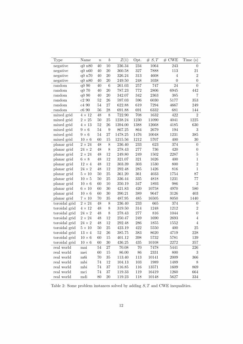
In the second experiment we examine the effect of using S, T -inequalitiesand CWE inequalities in addition to the star and triangle inequalities. Table 2presents several problem instances for which integer optimal LP solutions areobtained by using S, T inequalities and CWE inequalities. The column labelledZ(1) shows the LP value when all star and triangle inequalities are satisfied,so the difference between this value and Opt. is the gap that is closed by usingthe additional inequalities. The columns labelled # S, T and # CWE show thenumbers of S, T inequalities (including triangle inequalities) and CWE inequal-ities added to the LP during the optimization process. It is apparent from thetable that the time consumed by the cutting-plane algorithm has increased con-siderably in general when compared to the times in Table 1. It is also evidentthat there is a strong correlation between the number of inequalities neededand the time used. Again it is encouraging to see that several relatively largeproblem instances can be solved with just a few inequality classes and withoutbranching.

The next three experiments are aimed at evaluating the partial effects ofusing each of the classes of multistar, clique, and b-tree inequalities. Each ofthese inequality classes is used together with all classes of inequalities in thesecond experiment above, and only the still unsolved problem instances areconsidered. Below we present some results for the instances where one class ofinequalities dominates the others; that is, the LP value obtained on terminationof the cutting-plane algorithm is less than that obtained from using the otherinequalities.

There are a few problem instances for which the use of multistar inequalitiesgives tighter bounds than using clique or b-tree inequalities. The results areshown in Table 3. Here Z(2) is the bound that results from using S, T andCWE inequalities as in the second experiment, and Z(3) is the final LP valueobtained when multistar inequalities are also used. # MS is the total numberof multistar inequalities added. There is only one of these instances for whichan integer optimal LP solution is found. It should also be mentioned that thenumber of multistar inequalities added is sometimes quite modest in comparisonwith the other classes that are used. For example, in the planar grid 2 × 21instance more than 23,000 CWE inequalities are added, which explains therelatively long computation time.

The clique inequalities are sometimes very helpful to obtain good bounds;in particular when b is small relative to n. Using these inequalities we haveexperienced the best results for mixed grid and random instances. Some of theresults are shown in Table 4. Here Z(2) is as above and Z(4) is the final LPvalue that results from using the clique inequalities. # CL is the total number ofclique inequalities added to the LPs. In four of these instances integer optimalLP solutions are determined within a few seconds. In most of the remaininginstances considerable reductions in the gap between Z(2) and Opt. are obtainedwith reasonable computational effort. It is remarkable that only a few clique

10

Type Name n b Opt. Time (s)mixed grid 2× 20 40 10 648 0mixed grid 2× 20 40 20 884 14mixed grid 4× 10 40 20 938 9mixed grid 5× 8 40 20 938 8mixed grid 3× 14 42 21 996 16mixed grid 6× 7 42 21 996 25mixed grid 2× 22 44 22 1020 40mixed grid 2× 24 48 8 708 0mixed grid 2× 24 48 12 840 1mixed grid 3× 16 48 12 876 1mixed grid 4× 12 48 12 876 1mixed grid 8× 6 48 12 876 2mixed grid 2× 24 48 24 1164 99mixed grid 3× 16 48 24 1218 73mixed grid 4× 12 48 24 1336 65mixed grid 6× 8 48 24 1236 31mixed grid 5× 10 50 25 1320 39mixed grid 10× 6 60 30 1752 132mixed grid 10× 7 70 35 2234 373planar grid 23× 2 46 7 217 0planar grid 6× 8 48 24 355 4toroidal grid 2× 20 40 6 222 0toroidal grid 4× 10 40 20 329 3toroidal grid 5× 8 40 20 300 3toroidal grid 8× 5 40 20 293 1toroidal grid 3× 14 42 21 333 2toroidal grid 7× 6 42 21 329 3toroidal grid 21× 2 42 21 272 3toroidal grid 12× 4 48 8 350 0toroidal grid 4× 12 48 12 355 0toroidal grid 6× 8 48 12 354 1toroidal grid 4× 12 48 24 383 9toroidal grid 12× 4 48 24 412 4toroidal grid 6× 8 48 24 395 5toroidal grid 6× 10 60 30 474 23toroidal grid 7× 10 70 35 544 58real world mei 60 30 93 17real world mfi 90 15 131 7

Table 1: Some problem instances solved by using star and triangle inequalities.

11

Type Name n b Z(1) Opt. # S, T # CWE Time (s)negative q0 n80 40 10 236.34 234 1064 243 0negative q0 n60 40 20 360.58 327 7888 113 21negative q0 n70 40 20 326.24 313 4608 4 2negative q0 n80 40 20 249.50 248 1038 0 0random q0 90 40 6 261.03 257 747 24 0random q0 70 40 20 787.23 772 2806 6945 442random q0 90 40 20 342.07 342 2363 385 7random c2 90 52 26 597.03 596 6030 5177 353random c4 90 54 27 622.88 619 7294 4667 249random c6 90 56 28 691.88 691 6332 681 144mixed grid 4× 12 48 8 722.90 708 1632 422 2mixed grid 2× 25 50 25 1238.24 1230 11090 4041 1225mixed grid 4× 13 52 26 1394.00 1388 12668 4185 630mixed grid 9× 6 54 9 867.25 864 2679 194 3mixed grid 9× 6 54 27 1478.25 1476 10048 1231 385mixed grid 10× 6 60 15 1215.56 1212 5707 400 30planar grid 2× 24 48 8 236.40 233 623 374 0planar grid 24× 2 48 8 278.43 277 736 420 0planar grid 2× 24 48 12 249.80 249 1502 2287 5planar grid 6× 8 48 12 321.07 321 1626 400 1planar grid 12× 4 48 12 303.39 303 1530 800 2planar grid 24× 2 48 12 292.48 285 1426 816 1planar grid 5× 10 50 25 361.20 361 4033 1754 87planar grid 10× 5 50 25 336.44 335 4818 1231 77planar grid 10× 6 60 10 350.19 347 1893 986 2planar grid 6× 10 60 30 421.83 420 10758 4970 580planar grid 10× 6 60 30 390.21 389 9647 3126 403planar grid 7× 10 70 35 487.95 485 16505 8050 1440toroidal grid 2× 24 48 8 236.40 233 665 374 0toroidal grid 4× 12 48 8 319.50 314 1248 1212 2toroidal grid 24× 2 48 8 278.43 277 816 1044 0toroidal grid 2× 24 48 12 250.47 249 1690 2693 4toroidal grid 24× 2 48 12 292.48 286 1855 1552 4toroidal grid 5× 10 50 25 423.19 422 5550 400 25toroidal grid 13× 4 52 26 385.75 383 8620 4719 228toroidal grid 10× 6 60 15 401.12 398 5732 5781 139toroidal grid 10× 6 60 30 436.25 435 10108 2272 357real world mai 54 27 70.08 70 7478 5441 226real world mei 60 15 86.00 86 2331 800 3real world m6i 70 35 113.40 113 10141 2009 366real world mbi 74 12 104.13 103 1989 1489 8real world mbi 74 37 116.85 116 13571 1609 869real world mci 74 37 119.33 119 16419 1260 664real world mdi 80 20 119.23 118 10148 5627 334

Table 2: Some problem instances solved by adding S, T and CWE inequalities.

12

Type Name n b Z(2) Z(3) Opt. # MS Time (s)random t0 10 30 15 1071.01 1070.00 1070 334 560random t0 50 30 15 713.39 712.72 712 287 179mixed grid 2× 21 42 7 565.98 564.79 558 2565 390mixed grid 3× 14 42 7 572.36 570.00 558 984 59mixed grid 4× 11 44 11 746.41 745.20 742 367 57mixed grid 4× 13 52 13 968.93 967.66 960 1813 596planar grid 5× 8 40 6 199.80 199.21 199 549 3planar grid 2× 21 42 21 959.10 951.35 949 602 3589toroidal grid 8× 4 32 5 180.85 179.71 178 562 1

Table 3: Problem instances with best bounds from using multistar inequalities.

inequalities seem to be needed in order to enforce the bound reductions.Like the clique inequalities, the b-tree inequalities are also very useful to

obtain good bounds. Table 5 presents some of the results. Here Z(5) is the LPvalue that is reached by the cutting-plane algorithm when b-tree inequalities areused and # b-T is the total number of these inequalities that are added. In six ofthese problem instances an integer optimal LP solution is obtained, and in mostof the other instances an upper bound is obtained which is close to the valueof an optimal partition. There are, however, three instances (negative q0 n30,mixed grid 5× 8, and mixed grid 6× 7) where there is still a significant gap tobe closed. We note that relatively many b-tree inequalities are used to obtainthe bounds and that the cutting-plane algorithm runs through many iterationsin these cases, which is why the time spent by the algorithm often extends overseveral minutes.

The above results suggest that the classes of S, T , CWE, clique, and b-treeinequalities are the most useful of the five inequality classes that are consideredin this paper. Since, however, the multistar inequalities can be useful in someinstances we have chosen also to use them in our branch-and-cut algorithm. Weremark that our conclusion is based on the particular separation procedures wehave implemented for these inequality classes — better separation proceduresfor some classes may affect the outcome — so this conclusion is not a definiteone.

4.2 Branch-and-cut results

Here we present some computational results of the branch-and-cut algorithm.For each type of problem we consider a few of the larger instances with differentcluster capacities in order to demonstrate the size and range of problem instancesthat can be solved. In these experiments we have allowed the branch-and-cutalgorithm to run for a maximum of five hours. This means that some probleminstances have not been solved to proven optimality. Table 6 shows the results.The column labelled Heur shows the value of the best partition found by theheuristic. ZLP is the final LP value obtained at the root of the branch-and-cut enumeration tree. Branch is the number of subproblems considered duringthe enumeration; this includes the root problem so that a 1 in this columnmeans that the problem instance is solved without branching. Since all edgeweights are integers, a branch in the enumeration tree is pruned whenever the

13

Type Name n b Z(2) Z(4) Opt. # CL Time (s)random q0 00 40 6 718.45 700.66 687 3 21random q0 10 40 6 693.33 677.52 662 3 26random q0 20 40 6 664.19 650.01 632 2 25random q0 30 40 6 629.45 617.72 605 2 25random q0 40 40 6 589.56 579.95 567 2 21random q0 60 40 6 495.25 488.57 483 3 14random q0 70 40 6 426.29 422.48 416 2 9random q0 80 40 6 355.05 353.44 350 2 5random c0 70 50 8 674.34 672.81 666 2 130random c2 90 52 13 501.30 498.79 496 8 64mixed grid 2× 19 38 9 573.87 567.32 550 53 135mixed grid 2× 20 40 6 513.69 510.00 510 19 0mixed grid 4× 10 40 6 510.24 505.15 501 14 0mixed grid 5× 8 40 6 514.00 510.00 510 5 0mixed grid 2× 21 42 10 666.00 658.00 658 31 4mixed grid 3× 14 42 10 686.15 677.55 558 45 152mixed grid 6× 7 42 10 691.13 681.47 658 1 16mixed grid 2× 22 44 7 590.70 585.91 576 73 94mixed grid 4× 11 44 7 599.97 594.58 576 7 3mixed grid 2× 23 46 7 615.00 609.00 606 68 149mixed grid 2× 25 50 8 724.00 718.00 718 47 1mixed grid 5× 10 50 12 893.07 882.01 868 9 27mixed grid 4× 13 52 8 767.00 753.00 746 23 2

Table 4: Some problem instances with best bounds from using clique inequali-ties.

LP value exceeds the incumbent partition value by less than one. This is whyno branching takes place when ZLP < Heur + 1.

The negative and random problem instances have varying densities in termsof the number of nonzero edge weights. Our experience with these instancesshows that relatively dense instances are hard to solve, while the very sparseinstances are more easy to solve. The last two digits in the problem name givethe percentage of zero weights; for example, negative c0 n30 is relatively dense inthat only 30% of the edges have zero weights. We conclude that dense instanceswith 50 nodes or more cannot be solved within a reasonable time limit.

Despite the fact that some of the mixed grid instances are easily solved (cf.Tables 1 and 2), some of the other instances appear to be very hard to solve.For example, two of the instances in Table 6 cannot be solved within the 5-hour time limit. The reason is that these problem instances are very regularin structure — all edges in the grid have weight 10 and all other edges haveweight 1 — so that there exist several alternative optimal solutions. Sometimesthe gap between ZLP and the optimal partition value is large, and it may beextremely difficult to close this gap during the branch-and-cut enumeration.

We have been able to solve all the planar grid instances in the test set.Indeed, most of these instances are easily solved without branching when b =n/2 (a few examples are given in Tables 1 and 2). Table 6 gives some exampleswith smaller capacities b. All toroidal grid instances have also been solved.

14

Type Name n b Z(2) Z(5) Opt. # b-T Time (s)negative q0 n30 40 6 364.17 363.15 351 4778 80negative q0 n60 40 6 298.32 297.23 297 4486 62negative q0 n70 40 6 281.16 279.33 278 6964 210negative q0 n70 40 10 305.47 305.00 305 2443 71negative c0 n80 50 8 308.23 308.00 308 10329 1542random q0 90 40 10 292.06 291.09 288 2329 64random c0 90 50 8 403.65 402.51 402 7867 379mixed grid 5× 8 40 10 656.76 655.68 648 4994 364mixed grid 6× 7 42 7 577.23 575.77 558 6125 205mixed grid 6× 8 48 8 714.00 711.87 708 9504 910planar grid 4× 10 40 6 224.18 224.00 224 2685 27planar grid 8× 5 40 6 216.22 216.00 216 2481 11planar grid 10× 4 40 6 205.25 203.79 203 5399 97planar grid 4× 12 48 8 281.14 281.00 281 465 0toroidal grid 4× 10 40 6 240.72 238.62 237 2220 21toroidal grid 3× 14 42 7 272.09 270.91 270 7307 319toroidal grid 7× 6 42 7 267.28 265.66 265 6318 210toroidal grid 4× 11 44 11 323.37 323.00 323 1350 67toroidal grid 6× 8 48 8 316.91 315.82 314 6689 389

Table 5: Some problem instances with best bounds from using b-tree inequalities.

However, these instances seem to be somewhat harder to solve in general thanthe corresponding planar grid instances. The examples given in the table alsoindicate this; note that one instance is only barely solved within the 5-hour timelimit.

The set of real world problems contains the largest instances we have at-tempted to solve. The largest instance on 148 nodes is only solved for b = 74, inwhich case it is easily solved. For the smaller cluster capacities the algorithm isunable to solve the problem; in the case with b = 37 the cutting-plane algorithmdoes not complete its processing of the root problem within the time limit. Mostof the other problem instances in this set are solved without branching as canbe seen in Table 6.

5 Concluding remarks

The branch-and-cut algorithm presented in this paper works well on most prob-lem instances we have attempted to solve. In particular, this is true with regardto instances that are associated with grid graphs on 100 or fewer nodes. Withregard to the unstructured instances, however, the densities of the graphs to bepartitioned seem to be the single most deciding factor for the solvability of theproblems. In general, sparse problem instances are easily solved, while denseones are hard to solve — the latter instances may not be solved if the graph has50 nodes or more.

The cluster capacity b may also influence the ability to solve a problem.More than half of the instances that are easily solved without branching havecapacity b = n/2. Branching takes place more frequently when the capacities

15

Type Name n b Heur ZLP Opt. Branch Time (s)negative c0 n30 50 8 518 552.49 n.a. n.a. 18000negative c0 n40 50 8 556 571.55 556 95 2361negative c0 n50 50 8 504 522.11 504 157 3424negative c0 n30 50 12 561 590.98 561 361 13092negative c0 n40 50 12 571 600.88 571 301 8824negative c0 n50 50 12 536 564.19 542 93 3354negative c0 n30 50 25 582 593.26 582 33 1244negative c0 n40 50 25 575 599.97 577 115 3649negative c0 n50 50 25 549 570.34 549 95 2736random c0 70 50 8 666 674.29 666 27 813random c0 80 50 8 550 560.20 555 37 1565random c0 90 50 8 402 402.98 402 1 31random c0 70 50 12 792 828.23 n.a. n.a. 18000random c0 80 50 12 646 662.61 648 341 14651random c0 90 50 12 454 454.57 454 1 25random c0 70 50 25 1189 1233.32 1189 31 8539random c0 80 50 25 887 896.41 887 13 2218random c0 90 50 25 550 550.00 550 1 10mixed grid 2× 23 46 7 606 609.00 606 141 6194mixed grid 2× 23 46 11 734 752.00 n.a. n.a. 18000mixed grid 2× 23 46 23 1082 1084.15 1082 3 414mixed grid 5× 10 50 8 709 729.41 n.a. n.a. 18000mixed grid 5× 10 50 12 868 882.02 868 221 7490mixed grid 4× 13 52 8 746 753.00 746 629 4058mixed grid 4× 13 52 13 960 967.95 960 19 2341planar grid 5× 10 50 8 307 308.36 308 3 58planar grid 5× 10 50 12 333 334.18 333 3 110planar grid 6× 10 60 10 362 366.55 365 7 495planar grid 6× 10 60 15 388 392.31 389 19 4010planar grid 7× 10 70 11 433 434.37 434 3 376planar grid 7× 10 70 17 460 460.60 460 1 47toroidal grid 13× 4 52 8 319 319.81 319 1 2toroidal grid 13× 4 52 13 352 352.91 352 1 428toroidal grid 6× 10 60 10 386 390.24 386 33 1276toroidal grid 6× 10 60 15 419 420.65 420 3 168toroidal grid 7× 10 70 11 459 464.42 462 63 5505toroidal grid 7× 10 70 17 491 496.14 491 101 17616real world mdi 80 13 110 110.83 110 1 40real world mdi 80 40 125 125.77 125 1 6real world m1i 100 16 140 140.91 140 1 2real world m1i 100 25 145 145.97 145 1 221real world m1i 100 50 152 152.42 152 1 6real world m8i 148 24 230 231.66 n.a. n.a. 18000real world m8i 148 37 241 n.a. n.a. n.a. 18000real world m8i 148 74 258 258.61 258 1 84

Table 6: Some branch-and-cut results.

16

are smaller, but we cannot conlude that instances with small capacities areconsistently harder to solve than instances with larger capacities.

The fact that extensive branching sometimes takes place indicates that moreclasses of facet-defining inequalities may be needed in order to solve some ofthe hard problem instances. Whether some of the already known inequalityclasses from the literature can be useful in a branch-and-cut framework likethe present one is an open question that can only be answered through furthercomputational studies. Another important research direction is the search fornew classes of facets of Pn(b) and related polytopes.

References

[1] F. Barahona, M. Junger, G. Reinelt, Experiments in quadratic 0–1 pro-gramming, Mathematical Programming 44 (1989) 127–137.

[2] L. Brunetta, M. Conforti, G. Rinaldi, A branch-and-cut algorithm for theequicut problem, Mathematical Programming 78 (1997) 243–263.

[3] U. Faigle, R. Schrader, R. Suletzki, A cutting plane algorithm for optimalgraph partitioning, Methods of Operations Research 57 (1986) 109–116.

[4] C.E. Ferreira, A. Martin, C.C. de Souza, R. Weismantel, L.A. Wolsey, For-mulations and valid inequalities for the node capacitated graph partitioningproblem, Mathematical Programming 74 (1996) 247–266.

[5] C.E. Ferreira, A. Martin, C.C. de Souza, R. Weismantel, L.A. Wolsey,The node capacitated graph partitioning problem: A computational study,Mathematical Programming 81 (1998) 229-256.

[6] M. Grotschel, Y. Wakabayashi, A cutting plane algorithm for a clusteringproblem, Mathematical Programming 45 (1989) 56–96.

[7] M. Grotshcel, Y. Wakabayashi, Facets of the clique partitioning polytope,Mathematical Programming 47 (1990) 367–387.

[8] S. Holm, M.M. Sørensen, The optimal graph partitioning problem, ORSpektrum 15 (1993) 1–8.

[9] E.L. Johnson, A. Mehrotra, G.L. Nemhauser, Min-cut clustering, Mathe-matical Programming 62 (1993) 133–151.

[10] E.M. Macambira, C.C. de Souza, The edge-weighted clique problem: Validinequalities, facets and polyhedral computations, European Journal of Op-erational Research 123 (2000) 346–371.

[11] M.M. Sørensen, An adaptation of the Kernighan-Lin heuristic to the sim-ple graph partitioning problem, Working paper 99-1, Dept. of Manage-ment Science and Logistics, Aarhus School of Business, 1999. (Available atwww.hha.dk/∼mim/papers.htm.)

[12] M.M. Sørensen, Facet defining inequalities for the simple graph parti-tioning polytope, Working paper 00-3, Dept. of Management Science andLogistics, Aarhus School of Business, 2000. (Revised version available atwww.hha.dk/∼mim/papers.htm.)

17

[13] M.M. Sørensen, New facets and a branch-and-cut algorithm for theweighted clique problem, European Journal of Operational Research 154(2004) 57–70.

[14] M.M. Sørensen, b-Tree facets for the simple graph partitioning polytope,Journal of Combinatorial Optimization 8 (2004) 151–170.

[15] C.C. de Souza, M. Laurent, Some new classes of facets for the equicutpolytope, Discrete Applied Mathematics 62 (1995) 167–191.

18

Working Papers from Logistics/SCM Research Group L-2005-02 Michael M. Sørensen: Polyhedral computations for the simple graph

partitioning problem. L-2005-01 Ole Mortensen: Transportkoncepter og IT-støtte: et undersøgelsesoplæg og

nogle foreløbige resultater. L-2004-05 Lars Relund Nielsen, Daniele Pretolani & Kim Allan Andersen: K shortest

paths in stochastic time-dependent networks. L-2004-04 Lars Relund Nielsen, Daniele Pretolani & Kim Allan Andersen: Finding the

K shortest hyperpaths using reoptimization. L-2004-03 Søren Glud Johansen & Anders Thorstenson: The (r,q) policy for the lost-

sales inventory system when more than one order may be outstanding. L-2004-02 Erland Hejn Nielsen: Streams of events and performance of queuing sys-

tems: The basic anatomy of arrival/departure processes, when focus is set on autocorrelation.

L-2004-01 Jens Lysgaard: Reachability cuts for the vehicle routing problem with time

windows.

ISBN 87-7882-080-4

Department of Accounting, Finance and Logistics Faculty of Business Administration

Aarhus School of Business Fuglesangs Allé 4 DK-8210 Aarhus V - Denmark Tel. +45 89 48 66 88 Fax +45 86 15 01 88 www.asb.dk