Pollution-generating Technologies and Disposability ... · Pollution-generating Technologies and...

Pollution-generating Technologies andDisposability Assumptions

Arnaud Abad∗and Walter Briec∗

10es Journees de Recherches en Sciences Sociales 8 et 9 decembre2016

Abstract

This paper exams the concept of Pollution-generating Technologies (PgT).The main goal of this methodological contribution is to reveal any PgTin production processes compatible with a minimal set of assumptions.We model PgT using a congestion approach of the output set relaxingstrong disposability assumption. To this end, we define the B-disposalassumption, that is a kind of limited strong disposability. The B-disposalassumption reflects cost disposability assumption with respect to the un-desirable outputs. This disposability assumption leads to a new dualityresult between an output distance function and the revenue function withpossibly negative shadow prices. A sample of 13 representative Frenchairports is considered over the period 2007-2011, in order to implementthe new B-disposal assumption on non-parametric technologies.

JEL: C61, D24, Q50.

Keywords: B-disposal Assumption, Bad Outputs, Cost Disposability, Dis-tance Function, Duality, Pollution-generating Technologies (PgT), Revenue Func-tion.

∗University of Perpignan, CRESEM, 52 Avenue Paul Alduy, F-66860 PerpignanCedex, France. Corresponding author: [email protected], Phone: 0033 (0)430950480.

1

1 Introduction

Since the early nineties, researchers strive to model undesirable outputs1 us-

ing non-parametric models (Tyteca, 1996; Zhou et al., 2008a; Dakpo et al.,

2016). Such methods need less restrictive assumptions than the econometric

models (e.g. Murty and Kumar, 2003). Parametric methods involve to specify a

functional form while non-parametric models require to apply mathematical pro-

gramming methods; such as Data Envelopment Analysis (DEA). Furthermore,

non-parametric approach presents more flexibility (e.g., in terms of inputs and

outputs selection).

In general, several approaches are distinguished in the literature. Following

Scheel (2001), the proposed models can be classified either into direct or indi-

rect approaches. The former consider the original output data and alter the

technology assumptions whereas the latter modify the value of the undesirable

outputs.

The first approach was to treat bad outputs as inputs (Cropper and Oat-

tes, 1992; Reinhard et al., 2000; Hailu and Veeman, 2001; Sahoo et al., 2011;

Mahlberg et al., 2011). Fare and Grosskopf (2003) pointed out, through an illus-

trative example, that this method is inconsistent with physical laws. Following

Pethig (2003, 2006), this approach also fails to satisfy the Materials Balance Prin-

ciples (MBP)2. Moreover, considering residual outputs as inputs comes down to

model the technology with an unbounded output set (Fare and Grosskopf, 2003;

Leleu, 2013). Thus, this model fails to satisfy the standard axioms of produc-

tion theory. Furthermore, it does not consider the link between the undesirable

production and the inputs (Forsund, 2009).

1Note that throughout this paper we use equivalently the terms bad outputs, undesirableoutputs and residual outputs.

2More precisely, considering bad outputs as inputs fails to satisfy the first law of thermo-dynamics (Ayres and Kneese, 1969). This law can be illustrated through the famous sayingof one of the founder of modern chemistry: ”Nothing is lost, nothing is created, everything istransformed” Antoine Lavoisier (1743-1794).

2

The second approach attempts to model residual outputs in production the-

ory by introducing additional production axioms. Fare et al. (1989) introduced

model based on the concept of joint-production, using the Weak (or ray) Dis-

posability (WD) axiom proposed by Shepard (1970), and the null jointness as-

sumption. The former means that desirable and undesirable outputs can only

be simultaneously reduced by a proportional factor. The latter highlights the

pollution problem: any desirable production can be produced without bad out-

puts. Nevertheless, models derived from these notions have several limits. First,

they consider a single abatement factor. Kuosmanen (2005) proposed to en-

hance them by introducing a non-uniform abatement factor in order to capture

all feasible production plans. The traditional WD model, by considering a single

abatement factor, reduces the production set and thereby conduct to an artificial

high number of efficient Decision Making Units (DMUs). Second, the standard

WD model does not exclude positive shadow prices for residual outputs (Hailu

and Veeman, 2001; Hailu, 2003). Rodseth (2013) examines this issue, and finds

that positive prices may be appropriate in cases where bads are recuperated by

good outputs. Third, Kuosmanen and Podinovski (2009) pointed out that us-

ing a single abatement factor may yields some convexity infeasibilities. Finally,

Coelli et al. (2007) showed that WD model fails to satisfy the MBP.

There exist also indirect approaches which alter the value of undesirable out-

puts in order to transform them into desirable outputs. Several authors consider

an additive inverse transformation3 (Koopmans, 1951), and the translation in-

variance property (Ali and Seidford, 1990; Seidford and Zhu, 2002), while other

use a multiplicative inverse alteration (Golany and Roll, 1989). Then, stan-

dard DEA method can be implemented. However, as mentioned in Fare and

Grosskopf (2004), such approaches is not consistent with physical laws since it

3The additive inverse transformation consists to multiply each undesirable outputs by −1.This approach exhibits the same technology set as considering bad outputs as inputs. However,it alters the sign of undesirable outputs.

3

consider strong disposal of outputs. Another issue is that it difficult to determine

the suitable transformations of the bad outputs (Scheel, 2001).

Among the above approaches, WD models are extensively implemented in

the literature about non-parametric combined environmental and productive ef-

ficiency studies. With respect to the limits associated with the WD model,

two innovative approaches have been defined. First, an approach based on the

MBP was introduced (Lauwers, and Van Huylenbroeck, 2003; Coelli et al., 2007;

Lauwers, 2009). Most recently, Murty et al. (2012) proposed an innovative by-

production technology constructed as an intersection of an intended-production

technology and a residual-generation technology. Murty (2015) extended this

approach to a full-blown axiomatic model. Dakpo et al. (2016) presented a

critical review of these recent developments.

This paper proposes to model PgT using an innovative B-disposal assump-

tion. This approach is based upon the congestion of the output set for with a

relaxed disposability assumption is considered (Briec et al., 2016). We define

a new B-disposal assumption that is a sort of limited strong disposability. B-

disposal technologies allow to define congestion in the good outputs (i.e. loss of

good outputs) resulting from the output set does not satisfy the usual disposal

assumption. The B-disposal assumption reflects cost disposability assumption

with respect to the undesirable outputs. Cost disposability involves that it is not

possible to reduce freely bad outputs; i.e. without any costs. The main reason

for this methodological innovation is to reveal any PgT in production processes

compatible with a minimal set of assumptions. The basic tool employed to char-

acterize multi-output technologies is the output distance function. Being dual

to the revenue function (Shepard, 1953; Mc Fadden, 1978), it offers a general

framework to economy analysis.

This note unfolds as follows. Section 2 presents the traditional technology,

4

underlying standard axioms and their subsets. Furthermore, introduces the new

disposal assumption and the boundaries for the residual outputs. Section 3 high-

lights the notions of output distance function and revenue function on the new

PgT technology. Looking from a dual viewpoint, we establish the main duality

result between the output distance function and a revenue function allowing for

negative prices. Thereafter, we show how to detect cost disposability of unde-

sirable outputs and testing consistency with revenue maximization. Section 4

defines convex non-parametric PgT and proposes a non-parametric test of cost

disposability in bad outputs. A sample of 13 representative French airports is

considered over the period 2007-2011, in order to implement the new B-disposal

assumption on non-parametric technologies in section 5. Finally, Section 6 con-

cludes, discusses limitations and offers directions for future research.

2 Technology: Assumptions and Definitions

2.1 Technology Based upon Traditional Assumptions

Let us define the notation used in this paper: Rn+ be the non-negative Euclidean

n-dimensional orthant; for y, ν ∈ Rn+ we denote y ≤ ν ⇐⇒ yi ≤ νi ∀i ∈ [n],

where [n] denotes the subset {1, ..., n}.

A production technology transforming inputs x = (x1, ..., xm) ∈ Rm+ into

outputs y = (y1, ..., yn) ∈ Rn+ can be characterized by the output correspondence

P : Rm+ −→ 2R

n+ where P (x) is the set of all outputs vectors that can be produced

from x:

P (x) = {y : y can be produced from x} . (2.1)

Throughout this paper, we assume the output correspondence satisfies the

following regularity properties (see Hackman, 2008; Jacobsen, 1970; McFadden,

1978):

5

P1: P (0) = {0} and 0 ∈ P (x) for all x ∈ Rm+ .

P2: P (x) is bounded above for all x ∈ Rm+ .

P3: P (x) is closed for all x ∈ Rm+ .

Note that P1 imposes that there is no free lunch and that the null output

can always be produced. Moreover, P2 and P3 involve that P (x) is compact. In

addition to the axioms of no free lunch as well as the boundedness and closedness

of the output set, there are three other assumptions that we sometimes invoke

on the output correspondence:

P4: P (x) is a convex set for all x ∈ Rm+ .

P5 : If u ≥ x ⇒ P (x) ⊇ P (u).

P6: ∀y ∈ P (x), 0 ≤ v ≤ y ⇒ v ∈ P (x).

Assumption P4 postulates convexity of the output correspondence. This

is useful to provide a dual interpretation through the revenue function and in

empirical applications of, for instance, non-parametric technologies. Notice that

under P1 and P4 if y ∈ P (x) then λy ∈ P (x), ∀λ ∈ [0, 1]. This implies the

ray (or weak) disposability of the outputs, while axioms P5 and P6 imposes the

more traditional assumption of strong (or free) disposal of inputs and outputs. A

convex, ray disposable technology satisfying P1−P5 but failing P6 is congested

in the sense of Fare and Grosskopf (1983a).4

To measure efficiency, it is convenient to distinguish between certain subsets

of the output set P (x). In particular, two subsets denoting production units on

the boundary prove useful. For all x ∈ Rm+ , the efficient subset is defined by:

4Kuosmanen (2003) shows that this traditional specification fails convexity, but that arevised specification is convex.

6

E(x) = {y ∈ P (x) : v ≥ y and v = y ⇒ v ∈ P (x)}. (2.2)

The weak efficient subset is written as:

W (x) = {y ∈ P (x) : v > y ⇒ v ∈ P (x)}. (2.3)

2.2 Disposal Assumption for Bad Outputs

Let B ⊂ [n], indexing the bad outputs of the technology. We introduce the

following symbol:

y ≥B v ⇐⇒

⎧

⎪

⎨

⎪

⎩

yj ≤ vj if j ∈ B

yj ≥ vj else(2.4)

Moreover:

y >B v ⇐⇒

⎧

⎪

⎨

⎪

⎩

yj < vj if j ∈ B

yj > vj else(2.5)

Obviously, if −y ≥B −v we denote y ≤B v. Notice that if B = ∅, then we

retrieve the standard vector inequality, since the set of the residual outputs is

empty.

We can now define a new disposability assumption for the outputs.

Definition 2.1 Let P be an output correspondence satisfying P1-P3. For all

y ∈ Rn+, the output set P (x) satisfies the B-disposal assumption if for all sets

of output vectors{

yJ}

J∈{∅,B}⊂ P (x), y ≤J yJ for any J ∈ {∅, B} implies that

y ∈ P (x).

If B = ∅, then we retrieve B-disposal assumption reduces to the standard

free disposability assumption.

7

In this paper, the free disposal assumption is limited by combining it with

a particular partial reversion of free disposal. The more output dimensions are

subjected to these particular partial reversions of free disposability defined by the

B-disposal assumption, the more the traditional free disposability assumption

gets limited and thus weakened. Indeed, Definition 2.1 implies that the larger the

bad output subset B is the more difficult one can dispose outputs. In general,

these definitions can account for cases where there is a simultaneous lack of

free disposability in all dimensions, but it is also possible to define this lack

independently in several dimensions.

Let us introduce the following convex cone:

KB ={

y ∈ Rn : y ≥B 0

}

. (2.6)

Notice that this notation implies that K∅ = Rn+. Definition 2.1 is illustrated

in Figure 1. In the latter, we have B = {2}. For any y, if there is some yØ that

classically dominates y and some y2 that “{2}-dominates” y, then y ∈ P (x).

For a given configuration of observations, this serves to construct an output set

where wasting the second output (undesirable production) implies an additional

opportunity revenue in terms of the first output dimension (desirable produc-

tion). However, the reverse dependency between output dimensions does not

hold. The B-disposal assumption reflects cost disposability assumption with re-

spect to the bad outputs. Cost disposability implies that it is not possible to

reduce freely residual outputs (y2); i.e. without any costs.

8

✻

✲0

y1

y∅

y{2}

y

P (x)

y2 = Bad Output

−K{2}

Figure 1: The case B = {2} on an output set.

To study this new disposal assumption from a dual standpoint, we introduce

the revenue function R : Rn × Rm+ −→ R ∪ {−∞} defined by:

R(p, x) =

⎧

⎪

⎨

⎪

⎩

supy{p.y : y ∈ P (x)} if P (x) = ∅

−∞ if P (x) = ∅

(2.7)

Notice that this definition allows to take into account negative prices which

are specifically linked to PgT.

The following propositions study the properties of the B-disposal assumption.

Proposition 2.2 Let P be an output correspondence satisfying P1-P3. For all

x ∈ Rm+ , P (x) satisfies the B-disposal assumption if and only if:

P (x) =(

(P (x)− Rn+) ∩ (P (x)−KB)

)

∩ Rn+.

This proposition characterizes a B-disposal output set in terms of an in-

tersection of the convex cones in (2.6). Remark that 2.2 is only based on the

B-disposal assumption and P1-P3. Therefore, the above proposition holds true

even if P (x) is not convex.

The following proposition extends the results of Proposition 2.2 to a convex

output correspondence. In particular, we provide a dual characterization of the

9

B-disposability notion.

Proposition 2.3 Let P be an output correspondence satisfying P1-P3. More-

over, assume that P4 holds. For all x ∈ Rm+ , P (x) satisfies the B-disposal

assumption if and only if

P (x) ={

y ∈ Rn+ : p.y ≤ R(p, x), p ∈ R

n+ ∪KB

}

.

Intuitively stated, a convex output set satisfying B-disposal can be enveloped

by a revenue function for proper prices. This result constitutes the basis for the

duality result developed in Section 3.

We are now ready to define a new cost disposability notion in the dimension

of the residual outputs:

Definition 2.4 Let P be an output correspondence satisfying P1-P3 and let B

be a subset of [n]. For all x ∈ Rm+ , P (x) satisfies cost disposability of unde-

sirable outputs if it fails strong disposability assumption but satisfies B-disposal

assumption.

In particular this means that:

(P (x)− Rn+) ∩ R

n+ =

(

(P (x)− Rn+) ∩ (P (x)−KB)

)

∩ Rn+. (2.8)

Definition 2.4 provides a strict definition of cost disposability of bad outputs

by assuming that the output set does not satisfy the usual disposal assumption.

Recall that in such a case:

P (x) = (P (x)− Rn+) ∩ R

n+. (2.9)

In the following, for all price vector p ∈ Rn, we say that an output of P (x)

is p-optimal if it maximizes the revenue R(·, p). An output vector y ∈ P (x)

10

is interior, if y > 0. The next result establishes a characterization of the new

PgT.

Proposition 2.5 Let P be an output correspondence that satisfies P1-P3. As-

sume that P4 holds. P (x) satisfies cost disposability in the dimension of residual

outputs if and only if there exists some interior pB-optimal output in P (x) with

pB ∈ KB\Rn+.

2.3 Boundaries for Bad Outputs

It remains an open question: how to detect undesirable outputs from the struc-

ture of the output correspondence? To answer this question, it is useful to in-

troduce the concept of bad frontier. Therefore, the following definition identifies

a subset that is not efficient, but that is a part of the boundary of a B-disposal

output correspondence.

Definition 2.6 Let P be an output correspondence satisfying P1-P3 and let

B ⊂ [n]. For all x ∈ Rm+ , we call bad output efficient frontier the subset:

EB(x) = {y ∈ P (x) : v ≥B y and v = y ⇒ v ∈ P (x)}.

We call bad output weakly efficient frontier the subset:

WB(x) = {y ∈ P (x) : v >B y ⇒ v ∈ P (x)}.

It follows that E∅(x) = E(x) is the usual efficient subset of P (x). Moreover,

note that y ∈ EB(x) if and only if:

(P (x)\{y}) ∩ (y +KB) = ∅. (2.10)

11

Proposition 2.7 Let P be an output correspondence satisfying P1-P3. Assume

that P4 holds.

(a) The subsets EB(x) and WB(x) are closed.

(b) If the output set P (x) satisfies cost disposability with respect to residual out-

puts then the subset EB(x)\E(x) is non-empty and contains an interior point.

(c) Suppose that EB(x)\E(x) is non-empty and contains an interior point. Sup-

pose moreover that P (x) satisfies the B-disposal assumption. Then P (x) satisfies

cost disposability in the dimension of undesirable outputs.

Remark 2.8 There exist output sets that not satisfies cost disposability of bad

outputs and for which there exists a boundary point in EB(x)\E(x). For example

assume that P (x) is the cube defined by P (x) = {(y1, y2) ∈ R2+ : y1 ≤ 1, y2 ≤

1}. Then yB = (1, 0) ∈ E{1}\E. However, P (x) satisfies free disposability of

undesirable outputs.

3 Duality between Technology and Revenue Func-

tion Based on B-Disposability

Shephard (1953) introduced the so-called Shephard distance function in pro-

duction theory. This distance function characterises technology and provides

a useful tool in efficiency and productivity measurement by virtue of its radial

nature5. This distance function has the advantage to be always feasible under

P1-P4.5See Russell (1985, 1987) for an axiomatic approach to the measurement of technical effi-

ciency.

12

3.1 Distance Function and Revenue Function on PgT :

A Duality Result

The output distance function ψP : Rm+n+ −→ R ∪ {+∞} is defined by:

ψP (x, y) =

⎧

⎪

⎨

⎪

⎩

inf{λ > 0 : 1λy ∈ P (x)} if 1

λy ∈ P (x) for some λ > 0

+∞ otherwise(3.1)

The above definition holds for a technology that satisfies the ray disposability

assumption.

Following the traditional duality result in Jacobsen (1970) or McFadden

(1978) between revenue function and output distance function, one can state

a duality result making a link between the distance function and the revenue

function on an output set P (x) satisfying the ray disposability assumption.

Proposition 3.1 Let P be an output correspondence satisfying P1-P5 and P6.

We have the following properties:

(a) For all (x, y) ∈ Rm+n+

ψP (x, y) = infp≥0

{ p.y

R(p, x): R(p, x) = 0

}

. (3.2)

(b) Let p be a non-negative output price vector. We have:

R(p, x) = supy

{ p.y

ψ(x, y): y ∈ R

n+

}

. (3.3)

Apart from this traditional duality relationship, a weaker duality result be-

tween the revenue function and the ray (or weak) disposable output distance

function is available in the literature (e.g. Shephard (1974)) whereby some (but

not all) prices are allowed to be negative (assumption P6 is dropped).6

6Also McFadden (1978) anticipates the use of negative prices and maintains that duality

13

Now, we extend the properties of the distance function to account for negative

orientations and to be compatible with output sets satisfying the B-disposal

assumption.

Proposition 3.2 Let P be an output correspondence satisfying P1-P5. Assume

moreover that P (x) satisfies the B-disposal assumption. We have the following

properties:

(a) For all (x, y) ∈ Rm+n+ :

ψP (x, y) = infp∈KB∪Rn

+

{ p.y

R(p, x): R(p, x) = 0

}

. (3.4)

(b) Let p ∈ KB∪Rn+ be an output price vector having some negative components.

Then:

R(p, x) = supy

{ p.y

ψ(x, y): y ∈ R

n+

}

. (3.5)

Property (a) extends the results by Shephard (1953) in the context of an

output correspondence that may fail both the strong and the weak disposability

assumptions. The converse results expressing the revenue function with respect

to the Shephard distance function is stated in (b). This duality result consid-

erably weakens current duality results imposing strong disposability. Otherwise

stated, this proposition shows that B-disposal of outputs is a necessary and

sufficient condition for the output Shephard distance function to characterize

technology. This substantially weakens the existing result on the importance

of ray disposal in the outputs for the traditional output distance function to

characterize technology.

This new duality result is illustrated in Figure 2. Since the second output

satisfies cost disposability, it receives a negative price and the revenue function

ends up having a positive rather than a negative slope.

results can be preserved under these circumstances.

14

✻

✲0

y1

y

❥

P (x)

y2 = Bad Output

p.x = R(x, p)p.x

−K{2}

Figure 2: Shephard distance function and duality with B = {2} .

In principle it is possible to relax the convexity assumption. Under non-

convexity, the duality result in Proposition 3.2 would only hold locally (similar

to the local duality result in, e.g., Briec, Kerstens and Vanden Eeckaut (2004)).

Note again that while the revenue function is non-decreasing in the outputs,

revenue functions estimated on convex technologies are furthermore convex in

the outputs (see Jacobsen (1970) or Shephard (1974)).

It should be clear by now that when the output set satisfies free disposal, then

it also satisfies B-disposal assumption. But, the converse is not necessarily true.

The same applies to weak disposal assumption: an output set satisfying weak

disposability assumption also satisfies B-disposal assumption, but the converse

need not be true.

3.2 Measurement of Cost Disposability

We are now interested in making the link between special cases of the output

distance function introduced below and the cost disposability of bads. To study

this relationship from the dual viewpoint we introduce the adjusted price cor-

respondence p : Rm+n+ −→ 2R

ninspired from Luenberger (1995) and defined

15

by:

p(x, y) = arg minp∈KB∪Rn

+

{ p.y

R(p, x): R(p, x) = 0

}

. (3.6)

Notice that if the minimum is not achieved, then p(x, y) = ∅. At points where

ψP (x, ·) is differentiable and applying the envelop theorem to 3.4 we obtain:

∇yψP (x, y) =p(x, y)

R(p, x). (3.7)

Thus,

p(x, y) = ∇yψP (x, y)R(p, x) (3.8)

For simplicity, we introduce the following notation:

P ∅(x) = (P (x)−K∅) ∩ Rn+ = (P (x)− R

n+) ∩ R

n+, (3.9)

PB(x) = (P (x)−KB) ∩ Rn+, (3.10)

P J(x) = P ∅(x) ∩ PB(x) =(

(P (x)− Rn+) ∩ (P (x)−KB)

)

∩ Rn+. (3.11)

In the next proposition, the impact of adding convexity to axioms P1− P3

is analyzed.

Proposition 3.3 Let P be an output correspondence satisfying P1-P4. For all

x ∈ Rm+ , we have the following properties:

(a) P (x) satisfies cost disposability with respect to residual outputs if and only if

there exists some y ∈ P (x) such that p(x, y) ⊂ KB\Rn+.

(b) P (x) satisfies cost disposability in the dimension of undesirable outputs if

and only if there exists some y ∈ P (x) such that ψP ∅(x, y) < ψP J (x, y).

In the following a procedure is proposed to measure cost disposability in the

dimension of bads.

16

Definition 3.4 Let P be an output correspondence satisfying P1-P3. For all

production vector (x, y) ∈ T , we define the following ratio to measure cost dis-

posability of residual outputs:

DCB(x, y) = ψP J (x, y)/ψP ∅(x, y)

.

We can now state the following corollary for our measure of cost disposability

in the dimension of undesirable outputs.

Corollary 3.5 Let P be an output correspondence satisfying P1-P3. Assume

moreover that for all x ∈ Rm+ , P (x) satisfies the B-disposal assumption. Then,

there exists some y ∈ P (x) such that DCB(x, y) > 1 if and only if P (x) satisfies

cost disposability with respect to bad outputs.

This measure DCB(x, y) evaluates eventual cost disposability componentwise

per subset B.

3.3 Testing for Consistency with Revenue Maximization

Suppose we are given some data on input-output vectors (xj , yj) and output

prices pj for all j ∈ J . Here we ask whether or not there exists a family of

output sets P (x) that can make sense of this observed behavior. It is possible to

show that the existence of negative prices involves cost disposability of residual

outputs in the general sense defined in this contribution. Following Varian (1984)

we say that a family of output sets P (x) rationalizes the data if yj is a solution

of the program:

maxy

{

pj .y : y ∈ P (xj)}

(3.12)

17

for all j ∈ J . Equivalently, a family of output sets P (x) rationalizes the data if

for all j ∈ J and all y ∈ P (xj):

pj.yj ≥ pj.y. (3.13)

Assume that the output set is one-dimensional (n = 1). The main difference

with Varian’s (1984) Weak Axiom of Profit Maximization (WAPM) is that here

prices can be negative. This excludes the strong disposal (or negative monotonic)

property of the output set. Following Varian (1984) we assume the family of

output sets is nested by the following assumption:

∀y ∈ P (x), x ≤ u implies that y ∈ P (u). (3.14)

In the following, we suppose that for all j

pji < 0 if i ∈ B and pji > 0 if i /∈ B (3.15)

The key idea of the following result is that if an output set P (x) rationalizes the

data, then it necessarily satisfies a B-disposal assumption and cost disposability

assumption in the undesirable outputs dimension.

Proposition 3.6 The following conditions are equivalent:

(a) There exists a family of nested output sets P (x) that rationalizes the data.

(b) If xk ≤ xj, then pj.yk ≤ pj.yj for all j, k ∈ J .

(c) There exists a family of nontrivial closed, convex and nested output sets that

rationalizes the data and that satisfies cost disposability of bads.

An immediate consequence is that negative prices imply cost disposability

in the dimension of residual outputs. Obviously, if all observed prices are non-

negative, then we have B = ∅ for j ∈ J and, because of B = ∅, we retrieve the

18

Varian (1984) WAPM result.

Notice that in principle it is possible to relax the convexity assumption (e.g.,

as in Briec, Kerstens and Vanden Eeckaut (2004)). Obviously, the same remarks

as the ones mentioned at the end of subsection 3.1 apply.

4 Bad Outputs on Non-Parametric Technolo-

gies

In this section we focus on convex non-parametric technologies. In particular we

consider the so-called Data Envelopment Analysis (DEA) model due to Banker,

Charnes and Cooper (1984).

4.1 Non-Parametric Convex Technologies

We consider a set of DMUs A = {(xk, yk) : k ∈ K} where K is an index set of

natural number. We assume that the technology satisfy the Variable Returns

to Scale (VRS) assumption (Banker et. al., 1984)7. In such case the production

technology is defined by:

TDEA ={

(x, y) : x ≥∑

k∈K

µkxk, y ≤∑

k∈K

µkyk,∑

k∈K

µk = 1, µ ≥ 0}

(4.1)

For any observed (x0, y0), the output correspondence is:

7Notice that if we assume that A contains the null input-output vector (0, 0) then axiomP1 holds true. Equivalently, one can suppose a non-increasing returns to scale assumption(Fare et. al., 1983b).

19

PDEA(x0) ={

y : x0 ≥∑

k∈K

µkxk, y ≤∑

k∈K

µkyk,∑

k∈K

µk = 1, µ ≥ 0}

To establish cost disposability with respect to undesirable outputs, we need

to identify the following subset:

PB,DEA(x0) ={

y : x0 ≥∑

k∈K

θkxk, y ≤B∑

k∈K

θkyk,∑

k∈K

θk = 1, θ ≥ 0}

(4.2)

Let us consider the collection J = {∅, B}. We now have P J (x0) = P ∅ (x0) ∩

PB (x0) =(

(

P (x0)− Rn+

)

∩(

P (x0)−KB)

)

∩ Rn+. Equivalently, we have:

P J,DEA (x0) = PDEA (x0) ∩ PB,DEA (x0) (4.3)

Thus, we have8

8As mentioned previously, one can define non-convex B-disposal technologies:

P J,DEANC (x0) =

{

y : x0 ≥∑

k∈K

θkxk, x0 ≥∑

k∈K

µkxk

y ≤B∑

k∈K

θkyk, y ≤∑

k∈K

µkyk

θ, µ ∈ {0, 1}}

. (4.4)

20

P J,DEA(x0) ={

y : x0 ≥∑

k∈K

θkxk, x0 ≥∑

k∈K

µkxk

y ≤B∑

k∈K

θkyk, y ≤∑

k∈K

µkyk

∑

k∈K

θk =∑

k∈K

µk = 1, θ, µ ≥ 0}

The above system of linear inequations can be formulated:

P J,DEA(x0) ={

y : x0,i ≥∑

k∈K

θkxk,i, i = 1, ..., m (4.5)

x0,i ≥∑

k∈K

µkxk,i, i = 1, ..., m

yj ≥∑

k∈K

θkyk,j, j ∈ B

yj ≤∑

k∈K

θkyk,j, j = 1, ..., n

yj ≤∑

k∈K

µkyk,j, j = 1, ..., n

∑

k∈K

θk =∑

k∈K

µk = 1, θ, µ ≥ 0}

Remark that, if θ = µ then the above output set shows non-disposabilty of

undesirable outputs (Kuosmanen, 2005). Following Leleu (2013), such repre-

sentation is an incorrect modeling of VRS assumption in traditional Shepard’s

weakly disposable technology. Nevertheless, this modeling has been implemented

21

in the literature (see for instance Picazo-Tadeo et al., 2005; Bilsel et al., 2014).

This contribution provides an innovative axiomatic characterization of the in-

correct modeling of VRS assumption in traditional Shepard’s weakly disposable

technology.

Notice that if we consider a set of DMUs A′= {(xk, yk), (xk, 0) : k ∈ K}9,

where K is an index set of natural number, we retrieve the correct way of lin-

earizing VRS Shepard’s weakly disposable technology proposed in Kuosmanen

(2005). Kuosmanen and Podinovski (2009), showed that this technology is the

smallest convex extension of Shepard’s weakly disposable technology. Based on

the initial work of Podinovski (2004), they highlighted that Kuosmanen tech-

nology is the correct minimum extrapolation technology that verified the stated

axioms. This modeling allows to consider proper abatement factor for each ob-

served activity. Furthermore, based on this modeling, a dual interpretation of

weak disposability is proposed in Kuosmanen and Matin (2011)10. This paper

offers a new axiomatic characterization of the Kuosmanen technology.

In the same vein, if we take A′

0 = {(xk, yk), (x0, 0) : k ∈ K}8, the above

output set corresponds to the correct way of linearizing VRS Shepard’s weakly

disposable technology proposed in Leleu (2013). This modeling also introduce a

dual interpretation of weak disposability.

9In such a case axiom P1 holds true.10Kuosmanen and Matin (2011) introduced the concept of ”limited liability condition” to

provide a dual interpretation of the weak disposability. If the maximum profit is not positiveand smaller than the sunk costs of inputs the ”limited liability condition” is not verified. Insuch a case, it is optimal to stop the production activity.

22

✻

✲

.................................

PB(x0)

0

y2

y1

AA′

D

D′C

C′′ C′

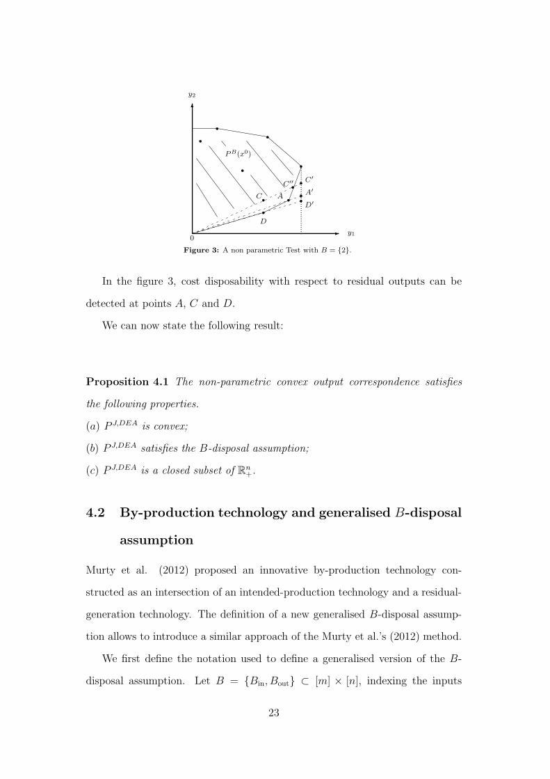
Figure 3: A non parametric Test with B = {2}.

In the figure 3, cost disposability with respect to residual outputs can be

detected at points A, C and D.

We can now state the following result:

Proposition 4.1 The non-parametric convex output correspondence satisfies

the following properties.

(a) P J,DEA is convex;

(b) P J,DEA satisfies the B-disposal assumption;

(c) P J,DEA is a closed subset of Rn+.

4.2 By-production technology and generalised B-disposal

assumption

Murty et al. (2012) proposed an innovative by-production technology con-

structed as an intersection of an intended-production technology and a residual-

generation technology. The definition of a new generalised B-disposal assump-

tion allows to introduce a similar approach of the Murty et al.’s (2012) method.

We first define the notation used to define a generalised version of the B-

disposal assumption. Let B = {Bin, Bout} ⊂ [m] × [n], indexing the inputs

23

generating pollution and the bad outputs of the technology. Let T a production

technology satisfying the following regularity properties:

T1: (0, 0) ∈ T and (0, y) ∈ T ⇒ y = 0.

T2: T (y) = {(u, v) ∈ T : v ≤ y} is bounded for all y ∈ Rn+.

T3: T is closed.

T4: ∀(x, y) ∈ T ∧ ∀(u, v) ∈ Rm+ × Rn

+ if (x,−y) ≤ (u,−v) then (u, v) ∈ T .

The assumptions T1−T3 are equivalent to P1−P3. T4 imposes traditional

assumption of strong disposability of inputs and outputs.

Definition 4.2 Let T a production technology satisfying T1-T3. For all (x, y) ∈

Rm+ ×Rn

+, the technology T satisfies the generalised B-disposal assumption if for

all sets of vectors{

xJ , yJ}

J∈{∅,B}⊂ T , (−x, y) ≤J (−xJ , yJ) for any J ∈ {∅, B}

implies that (x, y) ∈ T .

If B = ∅, then the generalised B-disposal assumption reduces to the standard

free disposability assumption (T4).

Proposition 4.3 Let T a technology satisfying T1-T3. For all (x, y) ∈ Rm+×Rn

+,

T satisfies the generalised B-disposal assumption if and only if:

T =(

(

T + (Rm+ × (−R

n+))

)

∩(

T + (KBin × (−KBout)))

)

∩ (Rm+ × R

n+).

For simplicity, we introduce the following notation:

T ∅ =(

T + (Rm+ × (−R

n+))

)

∩ (Rm+ × R

n+), (4.6)

TB =(


∩ (Rm+ × R

n+), (4.7)

24

T J = T ∅∩TB =(

(

T +(Rm+ × (−R

n+))

)

∩(

T +(KBin × (−KBout)))

)

∩ (Rm+ ×R

n+).

(4.8)

We assume that the technology satisfy the Variable Returns to Scale (VRS)

assumption (Banker et. al., 1984). To establish generalised cost disposability

with respect to polluting inputs and undesirable outputs, we need to identify

the following subset:

TB,DEA ={

(x, y) : x ≥Bin

∑

k∈K

θkxk, y ≤Bout∑

k∈K

θkyk,∑

k∈K

θk = 1, θ ≥ 0}

(4.9)

Let us consider the collection J = {∅, B}. We now have T J = T ∅ ∩ TB =(

(

T + (Rm+ × (−Rn

+)))

∩(


)

∩ (Rm+ ×Rn

+). Equivalently,

we have:

T J,DEA = TDEA ∩ TB,DEA (4.10)

Thus, we have

T J,DEA ={

(x, y) : x ≥∑

k∈K

µkxk, x ≥Bin

∑

k∈K

θkxk

y ≤∑

k∈K

µkyk, y ≤Bout

∑

k∈K

θkyk

∑

k∈K

θk =∑

k∈K

µk = 1, θ, µ ≥ 0}

The subset TB,DEA allows to capture cost disposability in the dimensions of

25

inputs generating pollution and residual outputs. In the Murty et al.’s (2012)

words, this sub-technology reflects nature’s residual generation. The subset

TDEA permits to capture the intended-production activities of firms. The in-

tersection of TB,DEA and TDEA defines a new PgT. Murty et al. (2012) assume

that the nature’s residual generation sub-technology operates independently of

the firm’s intended-production sub-technology. The proposed PgT no postulates

a such assumption. The subset TB,DEA is dependent on the intended (desirable)

outputs and on no polluting inputs; i.e., inequalities need to be specified for these

inputs and outputs in 4.9. We not assume that intended outputs and no-polluting

inputs not interact with the nature’s residual generation sub-technology. The

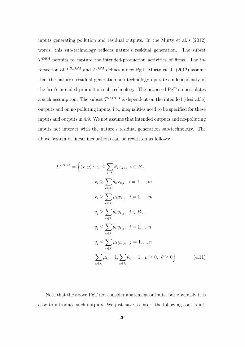
above system of linear inequations can be rewritten as follows:

T J,DEA ={

(x, y) : xi ≤∑

k∈K

θkxk,i, i ∈ Bin

xi ≥∑

k∈K

θkxk,i, i = 1, ..., m

xi ≥∑

k∈K

µkxk,i, i = 1, ..., m

yj ≥∑

k∈K

θkyk,j, j ∈ Bout

yj ≤∑

k∈K

θkyk,j, j = 1, ..., n

yj ≤∑

k∈K

µkyk,j, j = 1, ..., n

∑

k∈K

µk = 1,∑

k∈K

θk = 1, µ ≥ 0, θ ≥ 0}

(4.11)

Note that the above PgT not consider abatement outputs, but obviously it is

easy to introduce such outputs. We just have to insert the following constraint:

26

yj ≥∑

k∈K µkyk,j, j ∈ B′out. Where, B = {Bin, Bout, B′

out} ⊂ [m]× [n] indexing

the inputs generating pollution, the bad outputs and the abatement outputs of

the technology. Finally, remark that adding the following constraints11 in 4.11:

∑

k∈K

θkxk,i =∑

k∈K

µkxk,i, i = 1, ..., m

and

∑

k∈K

θkyk,j =∑

k∈K

µkyk,j, j = 1, ..., n.

Then, the PgT defined in 4.11 can be rewritten in the by-production tech-

nology (Murty et al., 2012).

4.3 Non-Parametric Test of Cost Disposability in the

Dimension of Bads

To test cost disposability with respect to undesirable outputs we need to be

able to compute the distance function over an output correspondence. From the

specification of convex non-parametric technologies, it is quite straightforward

to derive the following mathematical program12:

11These additional constraints assume that the efficient combination of the inputs and out-puts should be the same in both sub-technologies.

12Remark that, if θ = µ then ψPJ,DEA(x0, y0) can be implemented based on the set of DMUsA, A

′

or A′

0.

27

ψP J,DEA(x0, y0) = inf λ

s.t. x0,i ≥∑

k∈K

θkxk,i, i = 1, ..., m

x0,i ≥∑

k∈K

µkxk,i, i = 1, ..., m

1

λy0,j ≥

∑

k∈K

θkyk,j, j ∈ B

1

λy0,j ≤

∑

k∈K

θkyk,j, j = 1, ..., n

1

λy0,j ≤

∑

k∈K

µkyk,j, j = 1, ..., n

∑

k∈K

θk =∑

k∈K

µk = 1, θ, µ ≥ 0

The above program has 2(m+n) + 1+Card(B) constraints, where Card(B)

is the number of elements in B. When the technology is DEA convex, then the

solution is obtained by solving a linear program. To measure cost disposability

of residual outputs we need to compute ψP J,DEA(x0, y0)/ψPDEA(x0, y0)13. In the

same way ψPDEA(x0, y0) can be computed as follows:

13Consider replacing the VRS DEA technologies by CRS technologies and that θ = µ, thenthe test of cost disposability with respect to undesirable outputs is equivalent of the test ofcongestion in Fare et al. (1989) (not paying attention to the choice of distance function).

28

ψPDEA(x0, y0) = inf λ

s.t. x0,i ≥∑

k∈K

θkxk,i, i = 1, ..., m

1

λy0,j ≤

∑

k∈K

θkyk,j, j = 1, ..., n

∑

k∈K

θk = 1, θ ≥ 0

5 Empirical illustration

5.1 Data

The dataset used comes from many reports and documents of the Ministere de

l’ecologie, du Developpement durable et de l’Energie (http://www.developpement-

durable.gouv.fr). Two inputs are selected: (i) number of employees and (ii) oper-

ational costs. These inputs indicators permit to produce different outputs. Thus,

one desirable output, (iii) number of passengers ; and one undesirable output

represented by (iv) CO2 emissions. This bad output is measured by using the

TARMAAC (Traitements et Analyses des Rejets eMis dans l’Atmosphere par

l’Aviation Civile) tool of the Direction generale de l’Aviation civile (DGAC).

Table 1 presents the statistic descriptives of the variables used in this study.

5.2 Results

Table 2 presents measure of cost disposability in the dimension of residual out-

puts based on the B-disposability (DCB) and the weak disposability (DCWD)

29

Table 1: Characteristics of inputs and outputsVariables Min Max Mean St. Dev.

InputsEmployees (quantity) 67 3813 738 1166

Operational costs (Keuros) 15614 1112248 187521 329679Good Output

Passengers (quantity) 1014704 60970551 10328725 15646444Bad Output

CO2 emissions (millions of tons) 13 896 136 222

assumptions for the years 2007 to 2011.

Notice that both weak disposable and B-disposable Shepard output distance

functions are computed under VRS assumption (columns three and four). We

consider the correct linearization of the weakly disposable technology proposed

by Sahoo et al. (2011) or Zhou et al. (2008b):

ψPWD,DEA(x0, y0) = inf λ

s.t. x0,i ≥∑

k∈K

αkxk,i, i = 1, ..., m

1

λy0,j =

∑

k∈K

αkyk,j, j ∈ B

1

λy0,j ≤

∑

k∈K

αkyk,j, j = card(B) + 1, ..., n

∑

k∈K

αk = θ, α ≥ 0, 0 ≤ θ ≤ 1

Readers can see that the B-disposability assumption allows to consider a

more severe form of cost disposability with respect to undesirable outputs than

it proposed by the weak disposability assumption. For each time period we have:

Shep. BD ≥ Shep. WD or equivalently DCB ≥ DCWD.

30

Table 2: Measures of congestion in good outputsAirport Shep. SD Shep. WD Shep. BD DCWD DCB

2007

Bale-Mulhouse 0.7900 0.7900 0.7900 1.0000 1.0000Beauvais 0.6569 1.0000 1.0000 1.5224 1.5224

Bordeaux-Merignac 1.0000 1.0000 1.0000 1.0000 1.0000Lille 0.6419 0.6419 1.0000 1.0000 1.5578

Lyon-Saint Exupery 0.9091 0.9091 0.9091 1.0000 1.0000Marseille-Provence 0.9924 1.0000 1.0000 1.0077 1.0077

Montpellier-Mediterranee 0.7503 0.8927 1.0000 1.1898 1.3328Nantes-Atlantique 0.8713 0.8713 0.8811 1.0000 1.0113Nice-Cote d’azur 1.0000 1.0000 1.0000 1.0000 1.0000

Paris CDG 1.0000 1.0000 1.0000 1.0000 1.0000Paris ORY 0.5604 1.0000 1.0000 1.7844 1.7844

Strasbourg-Entzheim 1.0000 1.0000 1.0000 1.0000 1.0000Toulouse-Blagnac 1.0000 1.0000 1.0000 1.0000 1.0000

2008







2009







2010







2011







31

6 Conclusions

This paper is aimed to analyze the concept of PgT in the context of multi-output

production and duality theory. In this contribution a class of PgT based upon

a new notion of B-disposal assumption is considered. This new B-disposal as-

sumption consists to re-interpret the traditional strong disposability assumption

as a limited rather than a global property.

Thereafter, we introduce a new duality result between the output distance

function and the revenue function with possibly negative shadow prices. This

new duality result substantially weakens the existing result on the importance

of weak disposal in the outputs for the traditional output distance function to

characterize technology.

Then, introducing non parametric convex PgT, this contribution provides an

innovative axiomatic characterization of the incorrect modeling of VRS assump-

tion in traditional Shepard’s weakly disposable technology. Under specific sets

of DMUs (respectively A′and A

′

0), we retrieve the correct way of linearizing

VRS Shepard’s weakly disposable technology proposed in Kuosmanen (2005)

and Leleu (2013). Moreover, we show that the new PgT can be rewritten in the

by-production technology (Murty et al., 2012).

Finally, we propose an empirical illustration to emphasize the new measure

of cost disposability in the dimension of bad outputs (DCB). We show that

B-disposability assumption defines a more severe form of cost disposability with

respect to residual outputs than it suggested by the weak disposability assump-

tion.

The principal limitation of this paper relates of one main reason. We focus

on the output distance function and it dual relation with the revenue function.

The duality result and the new measure of cost disposability of bad outputs can

also defined using the so called directional distance function (Luenberger, 1992,

32

1995; Chambers et. al., 1996; Chambers and Pope, 1996).

33

References

Ali, A.I., L.M. Seidford (1990) Translation Invariance in Data Envelopment

Analysis, Operations Research Letters, 9, 403-405.

Ayres, R.U., A.V. Kneese (1969) Production, consumption, and externalities,

The American Economic Review, 59, 282-297.

Banker, R.D., Charnes, A., and W.W. Cooper (1984) Some Models for Estimat-

ing Technical and Scale Efficiency in Data Envelopment Analysis, Manage-

ment Science, 30, 1078-1092.

Bilsel, M., N. Davutyan (2014) Hospital efficiency with risk adjusted mortality

as undesirable output: the Turkish case Annal of Operational Research, 221,

73-88.

Briec, W., Kerstens, K., and P. Vanden Eeckaut (2004) Non-convex Technolo-

gies and Cost Functions: Definitions, Duality and Nonparametric Tests of

Convexity, Journal of Economics, 81(2), 155-192.

Briec, W., Kerstens, K., and I. Van de Woestyne (2016) Congestion in production

correspondences, Journal of Economics, 1-26.

Chambers, R., Chung, Y., and R. Fare (1996) Benefit and Distance Functions,

Journal of Economic Theory, 70(2), 407-419.

Chambers, R. G. and R. D. Pope (1996) Aggregate Productivity Measures,

American Journal of Agricultural Economics, 78: 1360-1365.

Coelli, T., Lauwers, L., and G. Van Huylenbroeck (2007) Environmental effi-

ciency measurement and the materials balance condition Journal of Produc-

tivity Analysis, 28, 3-12.

Cropper, M.L., and W.E. Oates (1992) Environmental Economics: A Survey,

Journal of Economic Literature, 30, 675-740.

Dakpo, K. H., Jeanneaux, P., and L. Latruffe (2016) Modelling pollution-generating

technologies in performance benchmarking: Recent developments, limits and

34

future prospects in the nonparametric framework, European Journal of Op-

erational Research, 250(2), 347-359.

Fare, R., and S. Grosskopf (1983a) Measuring output efficiencv, European Jour-

nal of Operational Research, 13, 173-179.

Fare, R., Grosskopf, S., and C.A.K. Lovell. (1983b) The Structure of Technical

Efficiency, Scandinavian Journal of Economics 85, 181-190.

Fare, R., Grosskopf, S., Lovell, C.A.K., and C. Pasurka (1989) Multilateral pro-

ductivity comparisons when some outputs are undesirable: A non parametric

approach, The Review of Economics and Statistics, 71, 90-98.

Fare, R., and S. Grosskopf (2003) NonParametric Production Analysis with Un-

desirable Outputs: Comment, American Journal of Agricultural Economics,

43(3), 257-271.

Fare, R., and S. Grosskopf (2004) Modeling Undesirable Factors in Efficiency

Evaluation: Comment, European Journal of Operational Research, 157, 242-

245.

Fare, R., and D. Primont (1995) Multi Output Production and Duality: Theory

and Applications, Kluwer Academic Publishers, Boston.

Forsund, F. R. (2009) Good Modeling of Bad Outputs: Pollution and Multiple-

Output Production, International Review of Environmental and Resource

Economics, 3, 1-38.

Golany, B., and Y. Roll (1989) An Application Procedure for DEA, Omega The

International Journal of Management Science, 17(3), 237-250.

Hackman, S.T. (2008) Production Economics: Integrating the Microeconomic

and Engineering Perspectives, Springer-Verlag Berlin Heidelberg.

Hailu, A., and T. S. Veeman (2001) Non-parametric Productivity Analysis with

Undesirable Outputs: An Application to the Canadian Pulp and Paper

Industry, American Journal of Agricultural Economics, 83(3), 605-616.

35

Hailu, A. (2003) Non-parametric Productivity Analysis with Undesirable Out-

puts: Reply, American Journal of Agricultural Economics, 85(4), 1075-1077.

Jacobsen, S.E. (1970) Production Correspondences, Econometrica, 38(5), 754-

771.

Koopmans, T. C. (1951) Analysis of Production as an Efficient Combination of

Activities, Activity Analysis of Production and Allocation, Cowles commis-

sion, Wiley and Sons, New York.

Kuosmanen, T. (2003) Duality Theory of Non-convex Technologies, Journal of

Productivity Analysis, 20(3), 273-304.

Kuosmanen, T. (2005) Weak Disposability in Nonparametric Production Analy-

sis with Undesirable Outputs, American Journal of Agricultural Economics,

87(4), 1077-1082.

Kuosmanen, T., and V. Podinovski (2009) Weak Disposability in Nonparametric

Production Analysis: Reply to Fare and Grosskopf, American Journal of

Agricultural Economics, 91(2), 539-545.

Kuosmanen, T., and R. K. Matin (2011) Duality of Weakly Disposable Technol-

ogy, Omega, 39, 504-512.

Lauwers, L., G. Van Huylenbroeck (2003) Materials balance based modelling

of environmental efficiency. In 25th international conference of agricultural

economist, South Africa.

Lauwers, L. (2009) Justifying the incorporation of the materials balance principle

into frontier-based eco-efficiency models, Ecological Economics, 68, 1605-

1614

Leleu, H. (2013) Shadow pricing of undesirable outputs in nonparametric anal-

ysis, European Journal of Operational Research, 231, 474-480.

Luenberger, D.G. (1992) Benefit Function and Duality, Journal of Mathematical

Economics, 21(5), 461-481.

36

Luenberger, D.G. (1995) Microeconomic Theory, Boston, McGraw-Hill.

Mahlberg, B., Luptacik, M., and B.K. Sahoo (2011) Examining the drivers of

total factor productivity change with an illustrative example of 14 EU coun-

tries, Ecological Economics, 72, 60-69.

McFadden, D. (1978) Cost, Revenue and Profit Functions, in: M. Fuss, D. Mc-

Fadden (eds) Production Economics: A Dual Approach to Theory and Ap-

plications, North-Holland publishing company, 3-109.

Murty, M.N., and S. Kumar (2003) Win-win opportunities and environmental

regulation: testing of porter hypothesis for Indian manufacturing industries,

Journal of Environmental Management, 67, 139-144.

Murty, S., Russell, R. R., and S. B. Levkoff (2012) On Modeling Pollution-

generating Technologies, Journal of Environmental Economics and Man-

agement, 64, 117-135.

Murty, S. (2015) On the properties of an emission-generating technology and its

parametric representation, Economic Theory, 60, 243-282.

Pethig, R. (2003) The ’materials balance approach’ to pollution: its origin, impli-

cations and acceptance, Universitt Siegen, Fakultt Wirtschaftswissenschaften,

Wirtschaftsinformatik und Wirtschaftsrecht in its series Volkswirtschaftliche

Diskussionsbeitrge, 105-03.

Pethig, R. (2006) Nonlinear Production, Abetment, Pollution and Materials Bal-

ance Reconsidered, Journal of Environmental Economics and Management,

51, 185-204.

Picazo-Tadeo, A. J., Reig-Martinez, E., and F. Hernandez-Sancho (2005) Di-

rectional Distance Functions and Environmental Regulation, Resource and

Energy Economics, 27, 131-142.

Podinovski, V. (2004) Bridging the Gap Between the Constant and Variable

Return-to-scale Models: Selective Proportionality in Data Envelopment Anal-

37

ysis, Journal of Operational Research Society, 55, 265-276.

Reinhard, S., Knox Lovell, C.A., and G.J. Thijssen (2000) Environmental Ef-

ficiency with Multiple Environmentally Detrimental Variables: Estimated

with SFA and DEA, European Journal of Operational Research, 121, 287-

303.

Rodseth, K. L. (2013) Capturing the least costly way of reducing pollution: A

shadow price approach, Ecological Economics, 92, 16-24.

Russell, R.R. (1985) Measures of Technical Efficiency, Journal of Economic The-

ory, 35, 109-126.

Russell, R.R. (1987) On the Axiomatic Approach to the Measurement of Techni-

cal Efficiency, Measurement in Economics: Theory and Application of Eco-

nomic Indices, W. Eichhorn Ed., Springer-Verlag Berlin Heidelberg.

Sahoo, B.K., Luptacik, M., and B. Mahlberg (2011) Alternative measures of en-

vironmental technology structure in DEA: An application, European Journal

of Operational Research, 275, 750-762.

Scheel, R.W. (2001) Undesirable Outputs in Efficiency Valuations, European

Journal of Operational Research, 132, 400-410.

Seidford, L., and J. Zhu (2002) Modeling Undesirable Factors in Efficiency Eval-

uation, European Journal of Operational Reaearch, 142, 16-20.

Shepard, R.W. (1953) Cost and Production Functions, Princeton: Princeton

University Press.

Shepard, R.W. (1970) Theory of Cost and Production Functions, Princeton:

Princeton University Press.

Shephard, R.W. (1974) Indirect Production Functions, Meisenheim am Glan,

Verlag Anton Hain.

Tyteca, D. (1996) On the Measurement of the Environmental Performance of

Firms - a Litterature Review and a Productive Efficiency Perspective, Jour-

38

nal of Environmental Management, 46, 281-308.

Varian, H. (1984) The Nonparametric Approach to Production Analysis, Econo-

metrica, 52(3), 579-597.

Zhou, P., Ang, B. W., and K. L. Poh (2008a) A survey of data envelopment anal-

ysis in energy and environmental studies, European Journal of Operational

Research, 189, 1-18.

Zhou, P., Ang, B. W., and K. L. Poh (2008b) Measuring environmental perfor-

mance under different environmental DEA technologies, Energy Economics,

30, 1-14.

39

Appendix:

Proof of Proposition 2.2: First, assume that P (x) satisfies the B-disposal

assumption. For all sets of output vectors{

yJ}

J∈{∅,B}⊂ P (x) and all y ∈ Rn

+,

y ≤J yJ ∀J ∈ {∅, B} implies that y ∈ P (x). Consequently, we deduce that

(⋂

J∈{∅,B} P (x) − KJ)⋂

Rn+ ⊂ P (x). Moreover, we obviously have P (x) ⊂

(⋂

J∈{∅,B} P (x) −KJ)⋂

Rn+. Hence, the first implication holds. Conversely, as-

sume that P (x) = (⋂

J∈{∅,B} P (x)−KJ)⋂

Rn+. For any J ∈ {∅, B}, if yJ ∈ P (x)

and y ≤J yJ , then y ∈ (P (x) − KJ)⋂

Rn+. Consequently, let a set of output

vectors{

yJ}

J∈{∅,B}⊂ P (x), y ∈ (P (x)−KJ)

⋂

Rn+ = P (x). Thus, P (x) satisfies

the B-disposal assumption. ✷

Proof of Proposition 2.3: We have P (x) = (⋂

J∈{∅,B} P (x)−KJ)⋂

Rn+. But,

for any J ∈ {∅, B} (since P4 holds),

P (x)−KJ =⋂

p∈KJ

{

y ∈ Rn+ : p.y ≤ R(p, x)

}

Consequently,

P (x) =(

⋂

J∈{∅,B}

⋂

p∈KJ

{y ∈ Rn+ : p.y ≤ R(p, x)}

)

∩ Rn+.

This subset can immediately be rewritten as:

P (x) ={

y ∈ Rn+ : p.y ≤ R(p, x), p ∈

⋃

J∈{∅,B}

KJ}

.

By using Proposition 2.2, this ends the proof. ✷

Proof of Proposition 2.5: We first prove that if there exists a price p ∈

KB\Rn+ and an interior pB-optimal output vector, then the technology satisfies

40

cost disposability in the dimension of bad outputs. Suppose that p ∈ KB\Rn+.

In such a case, there is some j ∈ [n]\B such that pj < 0. Assume that the

free disposal assumption holds and let us show a contradiction. Since P (x) is

a compact subset of Rn+, there exists some yB maximizing the revenue. Since

pj < 0 and under a free disposal assumption, at the optimum, we have yBj = 0.

Therefore, yB is not an interior point. Consequently, if there exists a pB-optimal

interior point, the output set is not freely disposable. Thus the output set P (x)

satisfies cost disposability with respect to undesirable outputs.

Let us prove the converse. Suppose that the output set satisfies cost dispos-

ability in the dimension of residual outputs. In such a case there exists some

frontier point zB > 0 that belongs to P (x) and some price vector rB ∈ KB\Rn+

such that zB maximizes the revenue for price rB. In the following we prove that

in the case where rB ∈ Rn+ one can find a pair (yB, pB) such that that yB is an

interior pB-optimal point with pB ∈ KB\Rn+. Since P (x) is closed, convex and

contains 0 and using the fact that zB > 0, it is easy to show that one can find

some frontier output vector yB > 0 in P (x). Moreover, from the hyperplane

support theorem there exists some price vector pB ∈ Rn with pB.yB = R(pB, x).

Clearly pB /∈ Rn+ because in such case we would have pB.y⋆ > pB.yB, which

contradicts the fact that yB maximizes the revenue.

We have proven that one can find a pair (yB, pB) such that yB > 0 is pB-

optimal with pB /∈ Rn+. Hence, all we need to prove is that pB ∈ KB. Suppose

this is not the case end let us show a contradiction. If this is not true, there is

some j ∈ B with pBj < 0. Let us consider the output vector yB defined for all

i ∈ [n] by

yBi =

⎧

⎪

⎨

⎪

⎩

yBi if i = j

0 if i = j

We obviously have yB ≤B yB. Since the B-disposal assumption holds yB ∈ P (x).

41

However, since pBj < 0, we have pB.yB > pB.yB that is a contradiction. There-

fore, pBi ≥ 0 for all i ∈ B which implies that pB ∈ KB and ends the proof. ✷

Proof of Proposition 2.7: (a) is a standard result whose the proof similar

to that one of the standard case. (b) Suppose that the technology satisfies cost

disposability with respect to bad outputs. From Proposition 2.5 there is an inte-

rior output vector yB ∈ P (x) and a price pB ∈ KB such that yB maximizes the

revenue in P (x). Since pB ∈ KB, the hyperplane {y : pB · y = R(x, pB)} weakly

separates P (x) and yB+KB. It follows that (P (x)\{yB})∩(yB+KB) = ∅. Con-

sequently, yB ∈ EB(x) which proves (b). To prove (c) suppose that there is some

zB ∈ EB(x) in the interior of P (x). Equivalently, (P (x)\{zB})∩ (zB +KB) = ∅.

From the convex separation theorem there is some price vector rB such that the

hyperplane {z : rB.z = R(x, rB)} weakly separates P (x) and zB+KB. However,

from the Farkas lemma, this property implies that rB ∈ KB. If rB /∈ Rn+, then

from Proposition 2.5, the result is established. If this is not the case, since the

output set is closed convex and contains 0, following the method used in the

proof of Proposition 2.5 one can find a frontier point yB > 0 that is pB-optimal

with pB ∈ KB\Rn+, which ends the proof. ✷

Proof of Proposition 3.2: (a) We have

ψP (x, y) =

⎧

⎪

⎨

⎪

⎩

inf{λ > 0 : 1λy ∈ P (x)} if 1

λy ∈ P (x) for some λ > 0

∞ otherwise

But from Proposition 2.3:

42

P (x) ={

y ∈ Rn+ : p.y ≤ R(p, x), p ∈

⋃

J∈{∅,B}

KJ}

=⋂

p∈!

J∈{∅,B} KJ

{

y ∈ Rn+ : p.y ≤ R(p, x)

}

.

Let us denote:

ψOE(x, y) = inf{λ > 0 :py

λ≤ R(p, x)}

Now, we have the equality:

ψP (x, y) = inf{λ > 0 :1

λy ∈ P (x)}

= infp∈

!J∈{∅,B} K

J

{

inf{λ > 0 :py

λ≤ R(p, x)}

}

= infp∈

!J∈{∅,B} K

JψOE(x, y)

If R(p, x) = 0, an elementary calculus yields:

ψP (x, y) =p∗y

R(p, x)

Consequently,

ψP (x, y) = infp∈

!J∈{∅,B} K

JψOE(x, y)

= infp∈

!J∈{∅,B} K

J

{ py

R(p, x): R(p, x) = 0

}

.

(b) can be obtained in a way similar to Fare and Primont (1995). ✷

43

Proof of Proposition 3.3 : (a) follows from Proposition 2.5 and 3.2.b. (b)

P (x) satisfies cost disposability in the dimension of undesirable outputs if and

only if P ∅(x) = P J(x). However, for any output correspondence P , y ∈ P (x)

if and only if ψP (x, y) ≤ 1. Moreover, by definition P J(x) ⊂ P ∅(x) which

implies that ψP ∅(x, y) ≤ ψP J (x, y). Hence, P ∅(x) = P J(x) is equivalent to

ψP ∅(x, y) = ψP J (x, y). Consequently P (x) satisfies cost disposability with the

respect to residual outputs if and only if ψP ∅(x, y) < ψP J (x, y) for at least some

y ∈ P (x), which ends the proof. ✷

Proof of Proposition 3.6: (a) =⇒ (b) is established in Varian (1984). Let us

prove that (b) =⇒ (c). Define P (x) as the smallest convex subset satisfying the

B-disposal assumption and containing all the yi such that xi ≤ x. Namely, if

A(x) = {yi : xi ≤ x, i ∈ I}, then we have:

P (x) =(

Co(

A(x))

−K∅)

∩(

Co(

A(x))

−KB)

∩ Rn+.

If there are no xi ≤ x, then let P (x) = ∅. Since Co(

A(x))

is a convex polytope,(

Co(

A(x))

−KI)

∩Rn+ is a convex polytope for all I ∈ {∅, B}. Therefore P (x)

is a convex polytope. Consequently, from Proposition 2.2, P (x) satisfies an B-

disposal assumption. Let us prove that P (x) rationalizes the data. Since P (xi)

is a convex polytope we only need to demonstrate this for the vertices of P (xi).

But, the vertices of P (xi) are some subset of A(xi). Since all the xk’s in A(xi)

satisfy the relevant condition by condition (b) we deduce that P (x) rationalizes

the data. Finally, by construction P (x) is closed, convex and nested. The last

implication (c) =⇒ (a) is obvious since (c) is stronger than (a). ✷

Proof of Proposition 4.1: (a) The subset P J,DEA is the intersection of a finite

44

number of convex sets, thus it is convex. (b) holds by definition of P J,DEA. (c)

P J,DEA is intersection of a finite number of closed sets, hence it is closed. ✷

Proof of Proposition 4.3: Based on Proof of Proposition 2.2 the result is

immediate. ✷

45

Pollution-generating Technologies and Disposability ... · Pollution-generating Technologies and...

Documents

Transcript of Pollution-generating Technologies and Disposability ... · Pollution-generating Technologies and...