Politically feasible reforms of non-linear tax systems∗

Felix J. Bierbrauer† Pierre C. Boyer‡

January 2, 2019

Abstract

We develop a framework for a political economy analysis of tax reforms. We

document that most tax reforms give rise to tax cuts or tax increases that are a

monotonic function of income. We prove a median voter theorem for monotonic

reforms of non-linear tax systems. We then focus on simple reforms that involve

a change of the tax rates for incomes in a certain bracket. We characterize the

conditions under which such reforms are politically feasible. We also develop a

sufficient statistics approach that identifies whether a given tax system admits

reforms that are politically feasible.

Keywords: Non-linear income taxation; Tax reforms; Political economy; Optimal

taxation.

JEL classification: C72; D72; D82; H21.

∗We thank Marcus Berliant, Laurent Bouton, Micael Castanheira, Vidar Christiansen, Sebastien

Courtin, Allan Drazen, Antoine Ferey, Sidartha Gordon, Olivier Gossner, Hans Peter Gruner, Bard

Harstad, Emanuel Hansen, Bas Jacobs, Laurence Jacquet, Kai Konrad, Yukio Koriyama, Etienne

Lehmann, Jean-Baptiste Michau, Benny Moldovanu, Massimo Morelli, Abdoulaye Ndiaye, Andreas Pe-

ichl, Carlo Prato, Anasuya Raj, Alessandro Riboni, Dominik Sachs, Michael Sicsic, Laurent Simula,

Johannes Spinnewijn, Stefanie Stantcheva, Alain Trannoy, Aleh Tsyvinski, Paul-Armand Veillon, Mar-

ius Vogel, John Weymark, Nicolas Werquin, Jan Zapal, and Floris Zoutman. We also appreciate the

comments of seminar and conference audiences at Yale, Paris-Dauphine, Oslo, Cologne, CREST-Ecole

Polytechnique, Leuven, Caen, Mannheim, ENS-Lyon, Paris Fiscal Study Group, 3rd Belgian-Japanese

Public Finance Workshop in Louvain, Transatlantic Theory Workshop in Paris, CESifo Area Conference

on Public Sector Economics, PET 2017, Tax-Day at MPI Munich, 67th Annual Meeting of the French

Economic Association, Taxation Theory Conference in St. Louis, LMU Munich. Jakob Wegmann pro-

vided excellent research assistance. The authors gratefully acknowledge the Max Planck Institute in

Bonn for hospitality and financial support, and the Investissements d’Avenir (ANR-11-IDEX-0003/Labex

Ecodec/ANR-11-LABX-0047) and IPP (Paris) for financial support.†CMR - Center for Macroeconomic Research, University of Cologne, Albert-Magnus Platz, 50923

Koln, Germany. E-mail: bierbrauer@wiso.uni-koeln.de‡CREST, Ecole Polytechnique, 5, avenue Henry Le Chatelier, 91128 Palaiseau, France. E-mail:

pierre.boyer@polytechnique.edu

1 Introduction

We present a new approach for a political economy analysis of non-linear tax systems.

We focus on tax reforms. Our main results provide a characterization of tax reforms that

are politically feasible in the sense that a majority of individuals prefers the reform over

the status quo.

Previous literature has focussed on models of voting over tax schedules. The set

of non-linear tax policies is multi-dimensional policy space. Thus, the median voter’s

preferred policy is not a Condorcet winner. This complicates any analysis of voting over

non-linear tax schedules. One way of dealing with this complication is to restrict attention

to a subset of tax systems for which a median voter theorem applies.1 These restrictions

limit the scope for a comprehensive political economy analysis of top tax rates, earned

income tax credits, or taxes for the middle class.

Our main contributions are as follows: First, we prove a median voter theorem for

reforms of non-linear tax systems. The theorem applies to reforms that satisfy a mono-

tonicity condition. We document that this monotonicity condition is typically satisfied

in practical tax policy. The analysis of politically feasible reforms, moreover, provides

an explanation for the frequent observation that income tax schedules are more progres-

sive for middle incomes than for low or high incomes. Second, we discuss the relation

between reforms that are politically feasible and reforms that are attractive from a wel-

fare perspective. Thereby we contribute to bridging the gap between political economy

analyses of non-linear taxes and analyses of optimal welfare-maximizing taxes. Political

economy approaches frequently limit attention to a subset of tax systems for tractability,

whereas the normative literature seeks to avoid a priori restrictions on tax policies. A

focus on monotonic reforms makes it possible to analyse whether non-linear tax systems

can be reformed in way that is both politically feasible and welfare improving, or, whether

the status quo is efficient in the sense that the scope for politically feasible welfare im-

provements has been exhausted. Finally, we develop a sufficient statistics approach that

identifies politically feasible reforms empirically, given data on the actual tax policy, the

behavioral responses to taxation and the distribution of incomes.

A median voter theorem for monotonic tax reforms. We focus on monotonic tax

reforms, i.e. on reforms with the property that the difference between taxes due after the

reform and taxes due before the reform is a monotonic function of income. We prove a

median voter theorem according to which a monotonic reform is politically feasible if and

only if it is supported by the taxpayer with median income (Theorem 1). We moreover

1For instance, the well-known prediction due to Meltzer and Richard (1981) that tax rates are an

increasing function of the difference between median and average income is obtained by focussing on

linear income taxes.

1

document that, in practice, most tax reforms are monotonic.2 For instance, the tax cuts

under Bush (2001-2003) in the US and in the 80s under Thatcher in the UK involved

tax cuts for all incomes, with larger cuts for larger incomes. By our Theorem 1, if the

person with median income is among the beneficiaries of such a reform, a majority will

be in favor. Another example of a monotonic reform is one that involves higher taxes,

with increases that are a larger for “the rich.” For instance, the tax reforms in the UK in

2010 and in France in 2013 were of this type. Again, if the median voter appreciates the

reform, there is a majority in favor of it. In an extension of Theorem 1, we also provide

conditions under which reforms that are monotonic only for incomes above or below the

median income are politically feasible. This applies to reforms of the US income tax

under Clinton and Obama. Both involved lower taxes for low incomes and higher taxes

for high incomes.

Political feasibility and welfare. Monotonic reforms also play a prominent role in

the theory of welfare-maximizing taxation. Characterizations of optimal tax systems via

the perturbation method often look at the welfare implications of reforms that we refer

to as simple in what follows.3 A simple reform involves a small change of the marginal

tax rates for incomes that lie in a certain bracket.4 Welfare-maximizing approaches then

strike a balance between the distortions due to the increase of tax rates in the bracket

and the revenue due to the increased tax receipts from incomes above the bracket. A

characterization of welfare-optimal taxes can be obtained from the condition that there

must not exist a simple reform that yields welfare gains.

Thus, simple reforms have welfare implications that are well understood. Moreover,

they are monotonic so that Theorem 1 applies. Hence, by focussing on simple reforms we

can provide a more detailed analysis of how the set of politically feasible reforms relates

to the set of welfare-maximizing reforms. To see where the tension between welfare con-

siderations and political feasibility may come from, note that political feasibility requires

that a reform makes a sufficiently large number of individuals better off. Welfare consid-

erations, by contrast, tradeoff utility gains and losses of different individuals. A reform

that yields large gains to a small group of individuals and comes with small losses for

a large group can be welfare-improving, but might not be politically feasible. A reform

that has small gains for many and large costs for few might be politically feasible without

2We investigate a panel of 33 OECD countries and find that 78 percent of the tax reforms that took

place since the year 2000 were monotonic reforms. For the Unites States, the United Kingdom, and

France we also consider alternative data sources that allow us to cover a longer time horizon. This leads

to similar conclusions: the share of monotonic reforms is 80% for the US (period 1981-2016), 84% for

France (period 1916-2016), and 77% for the UK (period 1981-2016).3See Piketty (1997), Saez (2001), Golosov, Tsyvinski and Werquin (2014), or Jacquet and Lehmann

(2016).4Consequently, the tax payments of individuals with incomes in the bracket change linearly with their

income; and, once the endpoint of the bracket is reached, the extra tax burden stays constant. Thus, a

simple reform involves additional taxes that are a non-decreasing function of income.

2

being welfare-improving.

Theorem 2 provides a characterization of simple reforms that are politically feasible.5

It considers a Pareto efficient tax system as the status quo. The theorem shows that tax

cuts for below median incomes and tax increases for above median incomes are politically

feasible. To see the logic, consider first a bracket of below median incomes. Lowering

the marginal tax rates for incomes in this bracket leads to a tax cut for all individuals

with higher income, including all individuals with above median income. It also involves

a loss of tax revenue. If the status quo is efficient, then individuals with above median

income are net beneficiaries, i.e. their gain from the tax cut outweighs their loss from the

reduced tax revenue. Hence, there is a majority in favor of such a reform. Interestingly,

the reduced rates apply to below median incomes, but the majority support relies on

above median incomes. The mirror image is a reform that involves higher rates for above

median incomes and which is supported by all individuals with below median income.

This characterization implies a marked discontinuity at the median level of income.

Below, tax cuts are politically feasible. Above, higher tax rates are politically feasible.

This marked discontinuity suggests an explanation for the observation that actual tax

schedules often have a pronounced increase of marginal tax rates close to the median

income:6 if political economy forces push towards low tax rates below the median and

towards high tax rates above the median, then there has to be an intermediate range that

connects the low rates below the median with the high rates above the median.

As a corollary, Theorem 2 also provides an answer to the question whether a given tax

system can be reformed in way that is both welfare-improving and politically feasible. For

below median incomes, moving towards lower marginal tax rates is politically feasible.

If, according to a given welfare measure, tax rates are too high in the status quo, then

such a reform is also politically feasible. Otherwise, there is no simple reform that is

both welfare-improving and politically feasible. Analogously, raising marginal tax rates

is politically feasible for above median incomes. If tax rates are too low from a welfare

perspective, then such a reform also yields a welfare gain. If not, there is no simple reform

for above median incomes that is both welfare improving and politically feasible.

Identifying politically feasible reforms. We also show how to bring our analysis to

the data. An implication of our analysis is that we only need Pareto bounds for marginal

tax rates to identify simple reforms that are politically feasible. We build on sufficient

statistics approaches to the analysis of non-linear tax systems. Specifically, we derive both

upper and lower Pareto bounds for marginal tax rates. How tight these Pareto bounds are

5A caveat that applies to any approach based on small reforms is that it can only identify directions

for reform. While this is informative, it does not extend without further assumptions to large reforms,

see Kleven (2018).6In Section 6 we present evidence for the US and France. The Netherlands share this pattern, see

Jacobs, Jongen and Zoutman (2017). In Germany it is referred to as the “Mittelstandsbauch” (middle

class belly) of the income tax schedule.

3

depends on behavioral responses, in particular on the elasticity of taxable income (ETI).

There is an inverse elasticity logic at play: the lower this elasticity, the more permissive

are the Pareto bounds. Tax policy then has a larger room to maneuver in the sense

that marginal tax rates can be lowered or increased without violating Pareto efficiency.

We illustrate our approach using data for the United States, the United Kingdom, and

France. For these empirical cases, the upper Pareto bound gets close to the status quo

schedule for values of this elasticity that are discussed in the empirical literature. Thus,

the discussion about the appropriate value of the ETI has implications for whether taxes

on “the rich” can be increased in a politically feasible way. Low estimates suggest that

the answer is “yes”, high estimates suggest that the answer is “no”. The lower bound

does not give rise to such controversies. It is far away from the status quo for plausible

values of the ETI. Thus, marginal taxes on “the poor” can be lowered in a politically

feasible way.

Outlook. The remainder is organized as follows. The next section discusses related

literature. Section 3 presents evidence on monotonic reforms. The formal framework

is introduced in Section 4. Section 5 contains the median voter theorem for monotonic

reforms. The characterization of politically feasible reforms can be found in Section 6.

Section 7 discusses extensions of the median voter theorem for monotonic reforms to

models of taxation that are richer than our basic setup, a generic Mirrleesian framework.

Specifically, we consider the possibility to mix direct and indirect taxes as in Atkinson and

Stiglitz (1976), the possibility to add sources of heterogeneity among individuals such as

fixed costs of labor market participation or public goods preferences, and the possibility

that taxpayers seek to mitigate income differences that are due to luck as opposed to

effort, as in Alesina and Angeletos (2005). The last section contains concluding remarks.

Unless stated otherwise, proofs are relegated to the Appendix.

2 Related literature

Any political economy approach to non-linear income taxation faces the difficulty that

the set of non-linear tax schedules is a multi-dimensional policy space. With such a

policy space, the existence of a Condorcet winner is not to be expected. Many political

economy approaches to redistributive taxation deal with this complication by restricting

attention to a subset of tax systems in which a Condorcet winner can be found. The

advantage of this approach is that it allows for clear-cut political economy predictions.

The disadvantage is that the set of tax systems may become too small for an analysis that

is empirically appealing. We provide a more detailed discussion that relates our work to

this literature in what follows. The main difference is that we look at preferences over

tax reforms – as opposed to preferences over a subset of tax systems.

Well-known political economy approaches to redistributive income taxation use the

4

model of linear income taxation due to Sheshinski (1972). In this model, marginal tax

rates are the same for all levels of income and the resulting tax revenue is paid out as a

uniform lump-sum transfer. As has been shown by Roberts (1977), the median voter’s

preferred alternative is a Condorcet winner in the set of all linear income tax systems.

Gans and Smart (1996) note that the median voter theorem for linear taxation reflects

a more general result in social choice theory due to Rothstein (1990; 1991).7 Our work

is related in that we also draw on Rothstein’s insight to prove a median voter theorem,

albeit one that applies to tax reforms.

The analysis by Gans and Smart (1996) extends to a specific class of non-linear tax

systems, namely those that can be ordered according to their degree of progressivity.

Benabou (2000) uses this framework for a dynamic political economy analysis of re-

distributive taxation. Specifically, he focusses on tax systems with a constant rate of

progressivity, see also Heathcote, Storesletten and Violante (2017). We present median

voter results that also apply to reforms of tax systems in this class. A limitation of it

is that one cannot have varying degrees of progressivity for different income categories.

Progressivity often times is particularly pronounced for middle incomes.

Median voter theorems for linear income taxation have been widely used on the as-

sumption that voters are selfish. A prominent example is the analysis by Meltzer and

Richard (1981). The explanatory power of this framework was found to be limited – see,

for instance, the review in Acemoglu, Naidu, Restrepo and Robinson (2015) – and has

led to analyses in which the preferences for redistributive tax policies are also shaped by

prospects for upward mobility or a desire for a fair distribution of incomes.8 In Section 7

we extend our basic analysis and prove a median voter theorem for reforms of non-linear

tax systems that takes account of such demands for fairness.

Roell (2012), Bohn and Stuart (2013) and Brett and Weymark (2016; 2017) study

non-linear taxes in the citizen-candidate framework due to Osborne and Slivinski (1996)

and Besley and Coate (1997): citizens compete for office and lack powers of commitment.

An elected candidate will therefore implement her own preferred policy. Voting over

candidates is therefore equivalent to voting over the non-linear tax policies that the

different candidates’ would select if they could dictate tax policy. The median voter’s

preferred tax policy is a Condorcet winner in this set of selfishly optimal tax schedules.

The literature has also explored political economy approaches to non-linear taxation

that do not give rise to median voter results. Non-linear taxation has, for instance,

been squared with probabilistic voting, the political agency model of Barro (1973) and

Ferejohn (1986), or pork-barrel spending.9 Saez and Stantcheva (2016) study generalized

7An alternative condition for the validity of the median voter theorem is that preferences are single-

peaked, see Black (1948).8See, for instance, Piketty (1995), Benabou and Ok (2001), Alesina and Angeletos (2005), Benabou

and Tirole (2006), or Alesina, Stantcheva and Teso (2018).9See Farhi, Sleet, Werning and Yeltekin (2012), Scheuer and Wolitzky (2016), Acemoglu, Golosov and

Tsyvinski (2008; 2010), or Bierbrauer and Boyer (2016).

5

welfare functions with weights that may reflect such political equilibrium outcomes. In

this paper, we focus on tax reforms. Moreover, we do not analyze political competition as

a strategic game that gives rise to equilibrium tax policies. Our framework is, however,

consistent with such an approach. Game-theoretic models of political competition can be

used to generate predictions of how the political process selects from the set of politically

feasible reforms.

Pareto bounds for non-linear taxes play an important role in our characterization of

politically feasible tax reforms. Upper bounds have previously been derived by Werning

(2007) and Lorenz and Sachs (2016). Our work also contains the characterization of a

lower Pareto bound.

Our characterization of politically feasible reforms uses perturbation arguments akin

to those in the literature on welfare-maximizing tax systems. It complements both the

heuristic approaches due to Piketty (1997) and Saez (2001) and approaches that use func-

tional derivatives such as Golosov et al. (2014) and Jacquet and Lehmann (2016). Simple

reforms – i.e. small changes of marginal tax rates for incomes in a particular bracket –

play a prominent role for both. Such reforms induce discontinuities in the marginal tax

schedule and hence give rise to discontinuous behavioral responses. Heuristic approaches

proceed on the assumption that these discontinuities can be ignored provided that the

reform is “sufficiently small.” The work on functional derivatives uses well-behaved ap-

proximations of simple reforms to avoid discontinuities. We neither use heuristics nor

approximations. Instead, we explicitly compute functional derivatives in the presence of

bunching.

The focus on reforms links our work to an older literature in public finance that seeks

to complement the theory of optimal taxation – which characterizes welfare-maximizing

tax systems and has no role for current tax policy – by a theory of incremental changes

that apply to a given status quo, see Feldstein (1976). Weymark (1981), for instance,

studies the scope for Pareto-improving reforms of a commodity tax system. Guesnerie

(1995) provides a survey of this literature and contains an analysis of tax reforms that

emphasizes political economy forces, formalized as a requirement of coalition-proofness.

Our analysis goes beyond this earlier literature by combining results from social choice

theory on the validity of median voter theorems with the perturbation approach to the

analysis of non-linear tax systems.

3 Monotonic reforms

The focus on monotonic tax reforms enables a tractable political economy analysis of tax

reforms in subsequent sections. Here, we define monotonic reforms more formally and

argue that they play a prominent role in practical tax policy. Let T0 be the pre-reform

and T1 be the post-reform tax schedule. The tax reform is said to be monotonic over

a range of incomes Y ⊂ R+ if T1 − T0 is a monotonic function for y ∈ Y . Given a

6

cross-section distribution of income, we say that a reform is monotonic above (below) the

median if T1− T0 is a monotonic function for incomes above (below) the median income.

As will become clear, monotonicity at least above or below the median is key for our

median voter results.

Tax reforms in OECD countries are typically monotonic over the whole range of in-

comes, but there are also notable deviations from this pattern. Many of these deviations

are such, however, that monotonicity applies for incomes above or below the median.

Other deviations are such that the non-monotonicity is negligible in magnitude. In the

following, we explain how we arrive at these assertions. First, we analyze tax reforms in

OECD countries from 2000 to 2016. Second, for the Unites States, the United Kingdom,

and France we use additional sources to cover a longer time horizon and we look explicitly

at specific tax reforms that took place in these countries.

The OECD provides annual data on key parameters of the statutory personal in-

come tax systems of its member countries. In particular, it documents tax brackets and

marginal tax rates. We use this information to construct the corresponding tax func-

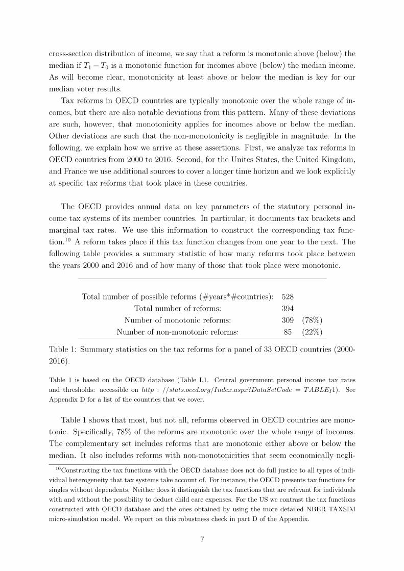
tion.10 A reform takes place if this tax function changes from one year to the next. The

following table provides a summary statistic of how many reforms took place between

the years 2000 and 2016 and of how many of those that took place were monotonic.

Total number of possible reforms (#years*#countries): 528

Total number of reforms: 394

Number of monotonic reforms: 309 (78%)

Number of non-monotonic reforms: 85 (22%)

Table 1: Summary statistics on the tax reforms for a panel of 33 OECD countries (2000-

2016).

Table 1 is based on the OECD database (Table I.1. Central government personal income tax rates

and thresholds: accessible on http : //stats.oecd.org/Index.aspx?DataSetCode = TABLEI1). See

Appendix D for a list of the countries that we cover.

Table 1 shows that most, but not all, reforms observed in OECD countries are mono-

tonic. Specifically, 78% of the reforms are monotonic over the whole range of incomes.

The complementary set includes reforms that are monotonic either above or below the

median. It also includes reforms with non-monotonicities that seem economically negli-

10Constructing the tax functions with the OECD database does not do full justice to all types of indi-

vidual heterogeneity that tax systems take account of. For instance, the OECD presents tax functions for

singles without dependents. Neither does it distinguish the tax functions that are relevant for individuals

with and without the possibility to deduct child care expenses. For the US we contrast the tax functions

constructed with OECD database and the ones obtained by using the more detailed NBER TAXSIM

micro-simulation model. We report on this robustness check in part D of the Appendix.

7

gible. We provide more specific examples of such reforms below. Not all countries have

a fraction of monotonic reforms close to the average of 78%. For instance, the fraction of

monotonic reforms is much smaller in Israel and Italy, and much larger in Belgium and

Sweden. Summary statistics for all OECD countries can be found in the supplementary

material for this paper. The Supplement also reports on findings obtained from additional

sources for the US, the UK and France. The share of monotonic reforms is 80% for the

US (period 1981-2016), 84% for France (period 1916-2016) and 77% for the UK (period

1981-2016). In the following, we illustrate these descriptive statistics by a discussion of

specific examples.

An interesting reform took place in France in 1937 (first budget after the Front Pop-

ulaire election in 1936). Figure 1 shows the reform induced change in the tax burden

for different levels of income. The origin of the sawtooth pattern is a change in the

description of the tax code. Tax law expressed tax liabilities by means of marginal tax

rates before the reform and by means of average tax rates after the reform. This example

illustrates that we tend to understate the prevalence of monotonic reforms by focussing

on the instances where T1 − T0 is a monotonic function: there are reforms, like the one

in the Figure, that are essentially monotonic even though the function T1 − T0 exhibits

some small non-monotonicities.

Figure 1: Reform of the French income tax in 1937

Examples of monotonic reforms are the tax cuts in the United Kingdom under the

Thatcher government in 1988, the 2010 reform in the United Kingdom and 2013 reform in

France that both involved the creation of a new bracket at the top, or the Bush tax cuts

between 2001 and 2003 in the United States that involved tax cuts that were increasing

in income (see Figure 2). The Reagan tax cuts are another example of a reform that

8

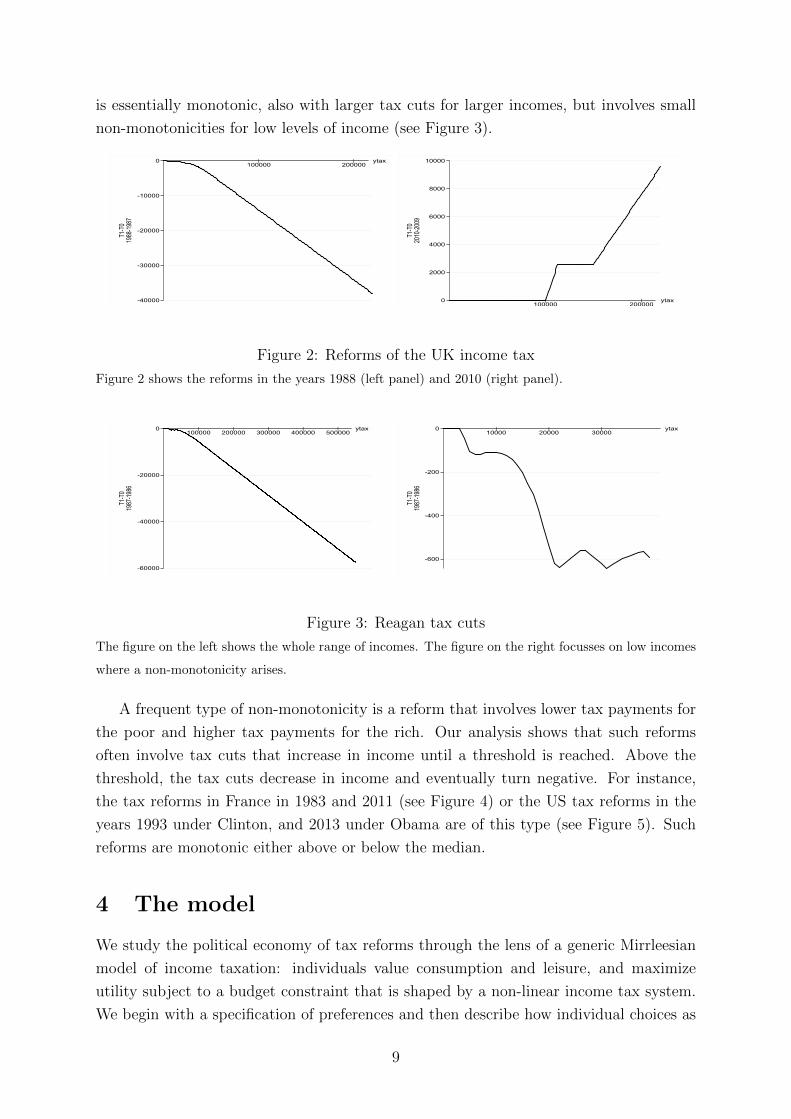
is essentially monotonic, also with larger tax cuts for larger incomes, but involves small

non-monotonicities for low levels of income (see Figure 3).

100000 200000| | ytax

-40000

-30000

-20000

-10000

0

T1-T

019

88-19

87

100000 200000| | ytax0

2000

4000

6000

8000

10000

T1-T

020

10-20

09

Figure 2: Reforms of the UK income tax

Figure 2 shows the reforms in the years 1988 (left panel) and 2010 (right panel).

100000 200000 300000 400000 500000| | | | | ytax

-60000

-40000

-20000

0

T1-T

019

87-19

86

10000 20000 30000| | | ytax

-600

-400

-200

0

T1-T

019

87-19

86

Figure 3: Reagan tax cuts

The figure on the left shows the whole range of incomes. The figure on the right focusses on low incomes

where a non-monotonicity arises.

A frequent type of non-monotonicity is a reform that involves lower tax payments for

the poor and higher tax payments for the rich. Our analysis shows that such reforms

often involve tax cuts that increase in income until a threshold is reached. Above the

threshold, the tax cuts decrease in income and eventually turn negative. For instance,

the tax reforms in France in 1983 and 2011 (see Figure 4) or the US tax reforms in the

years 1993 under Clinton, and 2013 under Obama are of this type (see Figure 5). Such

reforms are monotonic either above or below the median.

4 The model

We study the political economy of tax reforms through the lens of a generic Mirrleesian

model of income taxation: individuals value consumption and leisure, and maximize

utility subject to a budget constraint that is shaped by a non-linear income tax system.

We begin with a specification of preferences and then describe how individual choices as

9

100000 200000 300000 400000| | | | ytax

-4000

-2000

0

2000

4000

6000

T1-T

019

83-19

82

100000| ytax

-200

0

200

400

600

800

T1-T

020

11-20

10

Figure 4: Reforms of the French income tax in years 1983 and 2011

Figure 4 shows the reforms in the years 1983 (left) and 2011 (right).

50000 100000| | ytax

-500

0

500

1000

1500

T1-T

019

93-19

92

100000 200000 300000 400000 500000| | | | | ytax

-2000

0

2000

4000

6000

T1-T

020

13-20

12

Figure 5: Reforms of the US income tax under Clinton and Obama

Figure 5 shows the reforms in the years 1993 (left) and 2013 (right).

well as measures of tax revenue, welfare and political support are affected by reforms of

the tax system. We discuss extensions to richer models of taxation in Section 7.

4.1 Preferences

There is a continuum of individuals of measure 1. Individuals have a utility function u

that is increasing in private goods consumption, or after-tax income, c, and decreasing

in earnings or pre-tax income y. Individuals differ in their willingness to work harder in

exchange for increased consumption. To formalize this we distinguish different types of

individuals. The set of possible types is denoted by Ω with generic entry ω. The utility

that an individual with type ω derives from c and y is denoted by u(c, y, ω). The slope

of an individual’s indifference curve in a y-c-diagram −uy(c,y,ω)

uc(c,y,ω)measures how much extra

consumption an individual requires as a compensation for a marginally increased level of

pre-tax income. We assume that this quantity is decreasing in the individual’s type, i.e.

for any pair (c, y), and any pair (ω, ω′) with ω′ > ω,

−uy(c, y, ω′)

uc(c, y, ω′)≤ −uy(c, y, ω)

uc(c, y, ω).

10

This assumption is commonly referred to as the Spence-Mirrlees single crossing property.11

It implies that utility-maximizing choices are such that higher types end up having higher

incomes than lower types, and, in particular, that this ordering does not depend on the

tax system. Thus, type ω′ chooses weakly higher earnings than type ω < ω′ not only

under an initial tax schedule T0 but also under any alternative tax schedule T1.

The set Ω is taken to be a compact subset of the non-negative real numbers, Ω =

[ω, ω] ⊂ R+. The cross-section distribution of types in the population is represented by

a cumulative distribution function F with density f .

We allow for income effects. Specifically, we assume that leisure is a non-inferior

good. If individuals experience an increase in an exogenous source of income e, they do

not become more eager to work. More formally, we assume that for any pair (c, y), any

ω, and any e′ > e,

−uy(c+ e, y, ω)

uc(c+ e, y, ω)≤ −uy(c+ e′, y, ω)

uc(c+ e′, y, ω). (1)

The assumptions introduced so for are preserved by monotone transformations of the

individuals’ utility functions. Our analysis of politically feasible reforms does not require

anything else, i.e. it is based on an ordinal interpretation of the utility function u. When

performing welfare comparisons, we invoke the additional assumption that an individual’s

marginal utility of consumption uc(c, y, ω) is both non-increasing in c and non-increasing

in ω, i.e. ucc(c, y, ω) ≤ 0 and ucω(c, y, ω) ≤ 0.12 These assumptions will enable us to show

that the marginal consumption utility of low income types is not less than the marginal

consumption utility of high income types.

The Spence-Mirrlees single crossing property is an ordinal property, i.e. a property

that is preserved by monotone transformations of the utility function u. Higher types

have flatter indifference curves. The index ω represents this order. Any monotone trans-

formation of ω represents this order as well. Thus, as long as we only invoke the ordinal

properties of preferences, many representations of an individuals’ type are possible. This

observation will give us a degree of freedom when we bring our analysis of politically

feasible reforms to the data.

11The existing literature frequently invokes a utility function U : R2+ → R so that u(c, y, ω) = U

(c, yω

)and interprets ω as an hourly wage and l = y

ω as the time that an individual needs to generate a pre-tax-

income of y, see e.g. Mirrlees (1971) or Diamond (1998). Our analysis is consistent with this specification

but does not require it.12These assumptions hold for any utility function that is additively separable between utility from

consumption on the one hand and costs of effort on the other. With a non-separable utility function

of the form u(c, y, ω) = U(c, yω

), ucω(c, y, ω) ≤ 0 holds provided that Ucl

(c, yω

)≥ 0 so that working

harder makes one more eager to consume. Seade (1982) refers to Ucl(c, yω

)≥ 0 as non-Edgeworth

complementarity of leisure and consumption.

11

4.2 Tax reforms

Individuals are confronted with a predetermined income tax schedule T0 that assigns a

(possibly negative) tax payment T0(y) to every level of pre-tax income y ∈ R+. Under

the initial tax system individuals with no income receive a transfer equal to c0 ≥ 0. We

assume that T0 is everywhere differentiable so that marginal tax rates are well-defined

for all levels of income. We also assume that y − T0(y) is a non-decreasing function of y

and that T0(0) = 0.

A reform induces a new tax schedule T1 that is derived from T0 so that, for any level

of pre-tax income y, T1(y) = T0(y) + τ h(y), where τ is a scalar and h is a function.

We represent a reform by the pair (τ, h) where τ measures the size the reform. A small

reform, for instance, has τ close to zero. Without loss of generality, we focus on reforms

such that y−T1(y) is non-decreasing. The reform induces a change in tax revenue denoted

by ∆R(τ, h). For now we assume that this additional tax revenue is used to increase the

basic consumption level c0. Alternatives are considered in Section 7.

y

c

C1(y)

C0(y)

c0 + ∆R

c0

c0 + ∆R − τ(yb − ya)

ya yb

Figure 6: A simple reform

Simple reforms. Some of our results follow from looking at a special class of reforms.

For this class, there exists a first threshold level of income ya, so that the new and the

old tax schedule coincide for all income levels below the threshold, T0(y) = T1(y) for

all y ≤ ya. There exists a second threshold yb > ya so that, for all incomes between ya

and yb, marginal tax rates are increased (or decreased) by τ , T ′0(y) + τ = T ′1(y) for all

y ∈ (ya, yb). For all incomes above yb, marginal tax rates coincide, so that T ′0(y) = T ′1(y)

12

for all y ≥ yb. Hence, the function h is such that

h(y) =

0, if y ≤ ya ,

y − ya, if ya < y < yb ,

yb − ya, if y ≥ yb .

For reforms of this type we will write (τ, ya, yb) rather than (τ, h). Figure 6 shows how

a reform in the (τ, ya, yb)-class that generates positive tax revenue, ∆R > 0 , affects

the combinations of consumption c and earnings y that are available to individuals.

Specifically, the figure shows the curves

C0(y) = c0 + y − T0(y), and C1(y) = c0 + ∆R + y − T0(y)− τh(y) .

For incomes below ya and above yb the curves have the same slopes. The basic transfer

increases by ∆R so that more consumption is available at income levels smaller than ya.

Less consumption is available at income levels larger than yb. In Figure 6 we assumes that,

at these income levels, the loss from the additional tax payment τ(ya − yb) exceeds the

gain from the increase of the basic transfer.13 Between ya and yb the increased marginal

tax rate implies that the consumption schedule becomes flatter.

Simple reforms play a prominent role in the literature, see e.g. Saez (2001). By

contrast, analyses that use functional derivatives to analyze tax perturbations rest on

the assumption that both pre- and post-reform earnings are characterized by first order

conditions, see Golosov et al. (2014). Simple reforms cannot be approached directly with

this approach because they induce a discontinuity in marginal tax rates. Therefore, we

present a detailed analysis of the behavioral responses to simple reforms in part A of the

Appendix. The formal analysis that follows applies both to reforms in the (τ, ya, yb)-class

and to reforms where pre- and post-reform earnings follow from first order conditions.

Notation. To describe the implications of reforms for measures of revenue, welfare and

political support it proves useful to introduce the following optimization problem: choose

y so as to maximize

u (c0 + e+ y − T0(y)− τh(y), y, ω) , (2)

where e is a source of income that is exogenous from the individual’s perspective. We

assume that this optimization problem has, for each type ω, a unique solution that we

denote by y∗(e, τ, ω).14 The corresponding indirect utility level is denoted by V (e, τ, ω).

Armed with this notation we can express the reform-induced change in tax revenue as

∆R(τ, h) :=

∫ ω

ω

T1(y∗(∆R(τ, h), τ, ω))− T0(y∗(0, 0, ω))f(ω) dω .

13Otherwise the reform would be Pareto-improving, leading to additional consumption at all levels of

income.14For ease of exposition, we ignore the non-negativity constraint on y in the body of the text and

relegate this extension to part C in the Appendix. There, we clarify how the analysis has to be modified

if there is a set of unemployed individuals whose labor market participation might be affected by a

reform.

13

The reform-induced change in indirect utility for a type ω individual is given by

∆V (ω | τ, h) := V (∆R(τ, h), τ, ω)− V (0, 0, ω) .

Pareto-improving reforms. A reform (τ, h) is said to be Pareto-improving if, for all

ω ∈ Ω, ∆V (ω | τ, h) ≥ 0, and if this inequality is strict for some ω ∈ Ω.

Welfare-improving reforms. We consider a class of social welfare functions with

weights that are a non-increasing function g : Ω → R+. The welfare change that is

induced by a reform is given by

∆W (τ, h) :=

∫ ω

ω

g(ω)∆V (ω | τ, h)f(ω) dω .

A reform (τ, h) is said to be welfare-improving if ∆W (τ, h) > 0.

Political support for reforms. Political support for the reform is measured by the

mass of individuals who are made better if the initial tax schedule T0 is replaced by T1,

S(τ, h) :=

∫ ω

ω

1∆V (ω | τ, h) > 0f(ω) dω ,

where 1· is the indicator function. A reform (τ, h) is supported by a majority of the

population if S(τ, h) ≥ 12. We call such reforms politically feasible.

4.3 Types and earnings

We repeatedly invoke the function y0 : Ω→ R+ where y0(ω) = y∗(0, 0, ω) gives earnings

as a function of type in the status quo. We denote the inverse of this function by ω0 so

that ω0(y) is the type who earns an income of y in the status quo. By the Spence-Mirrlees

single crossing property the function y0 is weakly increasing. The existence of its inverse

ω0 requires in addition that, under the status quo schedule T0, there is no bunching so

that different types choose different levels of earnings.

Assumption 1 The function y0 is strictly increasing and continuous.

It is not difficult to relax this assumption. However, taking account of bunching in the

status quo requires additional steps in the formal analysis that we relegate to part C

of the Appendix. This extension is relevant because empirically observed tax schedules

frequently have kinks and hence give rise to bunching, see e.g. Saez (2010) and Kleven

(2016). That said, we focus on a status quo without bunching in the body of the text for

expositional clarity.

In much of the literature following Mirrlees (1971) types are identified with hourly

wages. Our framework is consistent with this approach, but is also compatible with

others. In particular, if y0 is a strictly increasing function then we can also identify

14

an individual’s type with the individual’s income in the status quo. This is particularly

useful for empirical applications. Information on the status quo distribution of incomes is

often more easily available than information on alternative measures of productive ability.

5 Median voter theorems for monotonic reforms

The focus on monotonic reforms enables a characterization of reforms that are politically

feasible. As we show in this section, checking whether or not a reform is supported by

a majority of individuals is, with some qualifications, the same as checking whether or

not the taxpayer with median income is a beneficiary of the reform. We begin with an

analysis of small reforms and turn to large reforms subsequently.

5.1 Small reforms

We say that an individual of type ω benefits from a marginal increase of τ if, at τ = 0,

∆Vτ (ω | τ, h) :=

d

dτV (∆R(τ, h), τ, ω) > 0 .

If this derivative is negative, we say that the individual benefits from a decrease of τ .

Theorem 1 Let h be a monotonic function. The following statements are equivalent:

1. The median voter benefits from a small reform.

2. There is a majority of voters who benefit from a small reform.

To obtain an intuitive understanding of Theorem 1, consider a policy-space in which indi-

viduals trade-off increased transfers and increased taxes. The following Lemma provides

a characterization of preferences over such reforms.

Lemma 1 Consider a τ -∆R diagram and let s0(ω) be the slope of a type ω individual’s

indifference curve through point (τ,∆R) = (0, 0). For any ω, s0(ω) = h(y0(ω)).

Consider, for the purpose of illustration, a reform in the (τ, ya, yb)-class. Individuals who

choose earnings below ya are not affected by the increase of tax rates. As a consequence,

s0(ω) = h(y0(ω)) = 0 which means that they are indifferent between a tax increase τ > 0

and increased transfers ∆R ≥ 0 only if ∆R = 0. As soon as τ > 0 and ∆R > 0, they are no

longer indifferent, but benefit from the reform. Individuals with higher levels of income

are affected by the increase of the marginal tax rate, and would be made worse off by any

reform with τ > 0 and ∆R = 0. Keeping them indifferent requires ∆R > 0 as reflected by

the observation that s0(ω) = h(y0(ω)) > 0. Moreover, if h is a non-decreasing function

of y, the higher an individual’s income the larger is the increase in ∆R that is needed

in order to compensate the individual for an increase of marginal tax rates. Noting that

y0(ω) is a non-decreasing function of ω by the Spence-Mirrlees single crossing property,

we obtain the following Corollary to Lemma 1.

15

Corollary 1 Suppose that h is a non-decreasing function of y. Then ω′ > ω, implies

y0(ω) ≤ y0(ω′) and s0(ω) ≤ s0(ω′) .

Corollary 1 establishes a single-crossing property for indifference curves in a τ -∆R-space,

see Figure 7 (right panel). The indifference curve of a richer individual is steeper than

the indifference curve of a poorer individual. Thus, if h is a non-decreasing function of y,

it is more difficult to convince richer individuals that a reform that involves higher taxes

and higher transfers is worthwhile. This is the driving force behind Theorem 1: if the

median voter likes such a reform, then anybody who earns less will also like it so that

the supporters of the reform constitute a majority. If the median voter prefers the status

quo over the reform, then anybody who earns more also prefers the status quo. Then,

the opponents of the reform constitute a majority.

y

c

IC(ω′)

IC(ω)

y

c

τ

∆R

IC(ω)

IC(ω′)

τ

∆R

Figure 7: Single-crossing properties

Figure 7 shows indifference curves of two types ω′ and ω with ω′ > ω. The figure on the left illustrates

the Spence-Mirrlees single-crossing property: in a y-c space lower types have steeper indifference curves

as they are less willing to increase their earnings in exchange for a given increase of their consumption

level. The figure on the right shows indifference curves in a τ -∆R space: here, lower types have flatter

indifference curves indicating that they are more willing to accept an increase of marginal taxes in

exchange for increased transfers.

The following Corollary uses these insights to provide a characterization of Pareto-

improving reforms and of reforms that are more controversial as they come with winners

and losers.

Corollary 2 Let h be a non-decreasing function.

(i) A small reform (τ, h) with τ > 0 is Pareto-improving if and only if the richest

individual is not made worse off, i.e. if and only if ∆Vτ (ω | 0, h) ≥ 0.

(ii) A small reform (τ, h) with τ < 0 is Pareto-improving if and only if the poorest

individual is not made worse off, i.e. if and only if ∆Vτ (ω | 0, h) ≤ 0.

16

(iii) A small reform (τ, h) with τ > 0 benefits voters in the bottom x per cent and harms

voters in the top 1− x per cent if and only if ∆Vτ (ωx | 0, h) = 0, where ωx satisfies

F (ωx) = x.

According to part (i) of Corollary 2, tax increases are Pareto-improving if and only if

the individuals with top incomes benefit. According to part (ii), tax cuts are Pareto-

improving if and only if they are in the interest of those with minimal income. Part

(iii) characterizes a reform that involves tax increases and which splits the population

into beneficiaries and opponents. If the individuals who just make it, say, to the top 10

per cent are indifferent then all individuals who belong to the bottom ninety percent are

winners and individuals in the top 10 per cent are losers.

Non-monotonic reforms. As shown in the previous section, not all conceivable re-

forms are such that h is monotone for all levels of income. For such reforms we cannot

prove an equivalence of support by the median voter and support by a majority of indi-

viduals. The following Proposition states a weaker result: it gives conditions under which

support of the median voter is a sufficient condition for political feasibility.

Proposition 1 Let y0M be median income in the status quo.

1. Let h be non-decreasing for y ≥ y0M . If the median voter benefits from a small

reform with τ < 0, then it is politically feasible.

2. Let h be non-decreasing for y ≤ y0M . If the poorest voter benefits from a small

reform with τ < 0, then it is politically feasible.

The first part of Proposition 1 covers reforms that are monotonic and involve tax cuts

that are more sizable for richer individuals, as under the Reagan and Bush tax cuts,

see Figure 3. A way of making sure that such a reform is appealing to a majority of

voters is to have the median voter among the beneficiaries. If, from the median voter’s

perspective, the reduced tax burden outweighs the loss of tax revenue, then everybody

with above median income benefits from the reform.

The second part applies the same logic to tax cuts for low incomes. If the poorest

individuals benefit from a tax cut and h is non-decreasing for below median incomes, then

individuals with incomes closer to the median benefit even more. Individuals with below

median incomes then constitute a majority in favor of the reform. This case applies,

in particular, to reforms so that T1 − T0 is negative and decreasing for incomes below

a threshold y, as for the reforms by Clinton and Obama, see Figure 5. In this case,

political feasibility is ensured by putting the threshold (weakly) above the median, so

that everybody with below median income is a beneficiary of the reform.

Heathcote et al. (2017) focus on income tax systems in a class that has a constant

rate of progressivity. A tax system in this class takes the form T (y) = y − λ y1−ρ where

the parameter ρ is the measure of progressivity and the parameter λ affects the level of

17

taxation. An increase of the rate of progressivity can be viewed as a reform (τ, h) so that

h is increasing for incomes above a threshold y and decreasing for incomes below y.15 As

a consequence, such a reform is monotonic either below or above the median.

The following Proposition that we state without proof demonstrates that the same

logic applies to reforms that involve higher taxes and higher transfers - rather than lower

taxes and lower transfers.

Proposition 2 Let y0M be median income in the status quo.

1. Let h be non-decreasing for y ≤ y0M . If the median voter benefits from a small

reform with τ > 0, then it is politically feasible.

2. Let h be non-decreasing for y ≥ y0M . If the richest voter benefits from a small

reform with τ > 0, then it is politically feasible.

5.2 Large reforms

We can evaluate the gains or losses form large reforms simply by integrating over the

gains and losses from small reforms since

∆V (ω | τ, h) =

∫ τ

0

∆Vτ (ω | s, h) ds . (3)

The following Lemma provides a characterization of the function ∆Vτ . The Lemma does

not require that a small reform is a departure from the status quo schedule with τ = 0.

It allows for the possibility that τ has already been raised from 0 to some value τ ′ > 0

and considers the implications of a further increase of τ .

Lemma 2 For all ω,

∆Vτ (ω | τ ′, h) = u1

c(ω)(∆Rτ (τ ′, h)− h(y1(ω))

), (4)

where u1c(ω) := uc

(c0 + ∆R(τ ′, h) + y1(ω)− T1(y1(ω)), y1(ω), ω

)is a shorthand for the

marginal utility of consumption that a type ω individual realizes after the reform and

y1(ω) := y∗(∆R(τ ′, h), τ ′, ω) is the corresponding earnings level.

If h is a monotonic function, then a reform’s impact on available consumption, as mea-

sured by ∆Rτ (τ ′, h)− h(y1(ω)), is a monotonic functions of ω. These observations enable

us to provide an extension of Theorem 1 to large reforms: if every marginal increase of τ

yields a gain ∆Rτ (τ ′, h)− h(y1(ω)) that is larger for less productive types, then a discrete

change of τ also yields a gain that is larger for less productive types. As a consequence,

if the median voter benefits if τ is raised from zero to some level τ ′ > 0, then anyone

15Formally, let the status quo be a tax system T0 with T0(y) = y−λ0y1−ρ0 . Consider the move to a new

tax system T1 with T1(y) = y−λ1y1−ρ1 and ρ1 > ρ0. Then τ h(y) = T1(y)−T0(y) = λ0y1−ρ0 −λ1y1−ρ1 .

This expression is strictly increasing in y for y > y :=(λ1(1−ρ1)λ0(1−τ0)

) 1ρ1−ρ0

and strictly decreasing for y < y.

18

with below-median income will also benefit. If the median voter does not benefit, then

anyone with above-median income will also oppose the reform. Consequently, a reform

is politically feasible if and only if it is in the median voter’s interest.

Proposition 3 Let h be a monotonic function.

1. Consider a reform (τ, h) so that for all τ ′ ∈ (0, τ), ∆Vτ (ωM | τ ′, h) > 0, then this

reform is politically feasible.

2. Consider a reform (τ, h) so that for all τ ′ ∈ (0, τ), ∆Vτ (ωM | τ ′, h) < 0, then this

reform is politically infeasible.

Propositions 1 and 2 also extend to large reforms with similar qualifications.

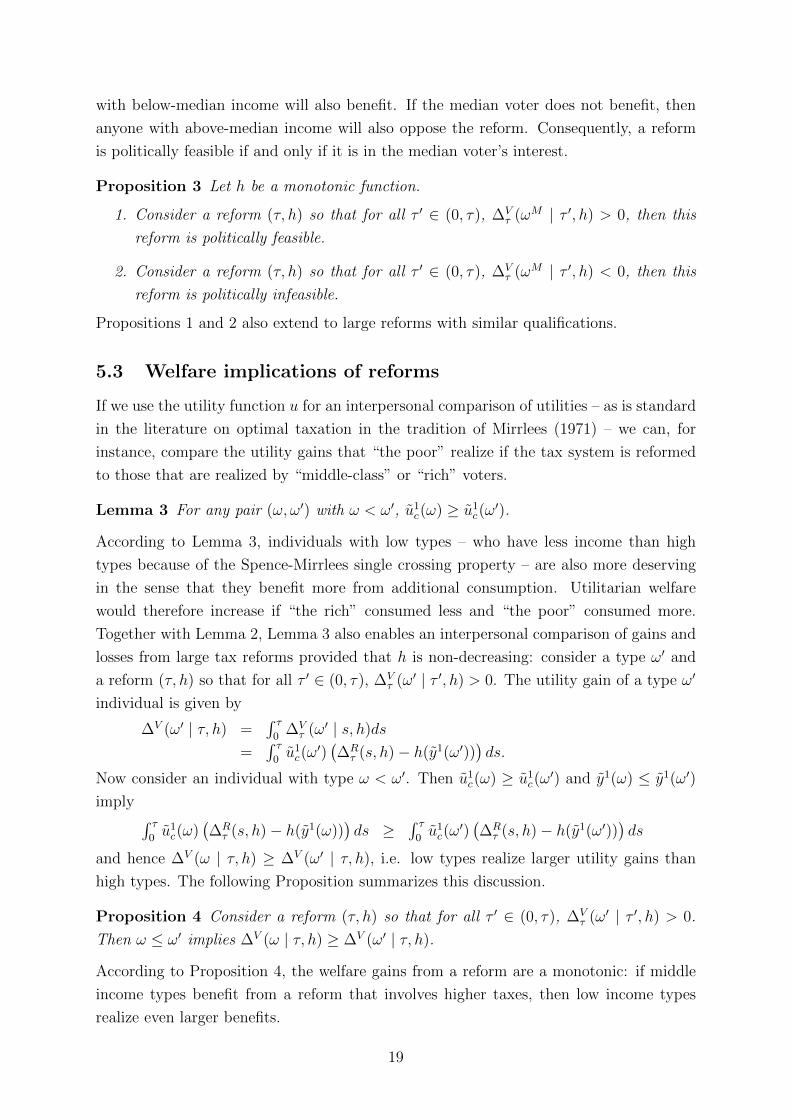
5.3 Welfare implications of reforms

If we use the utility function u for an interpersonal comparison of utilities – as is standard

in the literature on optimal taxation in the tradition of Mirrlees (1971) – we can, for

instance, compare the utility gains that “the poor” realize if the tax system is reformed

to those that are realized by “middle-class” or “rich” voters.

Lemma 3 For any pair (ω, ω′) with ω < ω′, u1c(ω) ≥ u1

c(ω′).

According to Lemma 3, individuals with low types – who have less income than high

types because of the Spence-Mirrlees single crossing property – are also more deserving

in the sense that they benefit more from additional consumption. Utilitarian welfare

would therefore increase if “the rich” consumed less and “the poor” consumed more.

Together with Lemma 2, Lemma 3 also enables an interpersonal comparison of gains and

losses from large tax reforms provided that h is non-decreasing: consider a type ω′ and

a reform (τ, h) so that for all τ ′ ∈ (0, τ), ∆Vτ (ω′ | τ ′, h) > 0. The utility gain of a type ω′

individual is given by

∆V (ω′ | τ, h) =∫ τ

0∆Vτ (ω′ | s, h)ds

=∫ τ

0u1c(ω

′)(∆Rτ (s, h)− h(y1(ω′))

)ds.

Now consider an individual with type ω < ω′. Then u1c(ω) ≥ u1

c(ω′) and y1(ω) ≤ y1(ω′)

imply ∫ τ0u1c(ω)

(∆Rτ (s, h)− h(y1(ω))

)ds ≥

∫ τ0u1c(ω

′)(∆Rτ (s, h)− h(y1(ω′))

)ds

and hence ∆V (ω | τ, h) ≥ ∆V (ω′ | τ, h), i.e. low types realize larger utility gains than

high types. The following Proposition summarizes this discussion.

Proposition 4 Consider a reform (τ, h) so that for all τ ′ ∈ (0, τ), ∆Vτ (ω′ | τ ′, h) > 0.

Then ω ≤ ω′ implies ∆V (ω | τ, h) ≥ ∆V (ω′ | τ, h).

According to Proposition 4, the welfare gains from a reform are a monotonic: if middle

income types benefit from a reform that involves higher taxes, then low income types

realize even larger benefits.

19

6 Detecting politically feasible reforms

By our median voter theorems, in order to understand whether there are politically

feasible reforms of a tax system we need to understand whether or not it can be reformed

in a way that makes the voter with median income better off. But how do we tell whether

or not a given tax system admits reforms that are in the median voter’s interest? In

this section, we first provide a characterization of such reforms (Theorem 2), and then

develop a sufficient statistics approach that makes it possible to identify them empirically.

Our analysis enable us to identify tax schedules that can be reformed in such a way

that the requirements of political feasibility and welfare improvements are both met.

Put differently, it makes it possible to identify tax schedules that are inefficient in the

sense that the scope for politically feasible welfare improvements has not been exhausted.

Throughout, we focus on simple reforms and provide sufficient conditions under which

such reforms are politically feasible and/ or welfare improving.

6.1 Pareto-efficient tax systems and politically feasible reforms

Theorem 2 below provides a characterization of simple reforms that are politically feasible.

Before we state the theorem, we introduce some terminology. A tax schedule T0 is Pareto-

efficient if there is no Pareto-improving reform. If it is Pareto-efficient, then for all ya

and yb,

yb − ya ≥ ∆Rτ (0, ya, yb) ≥ 0 ,

where ∆Rτ (0, ya, yb) is the marginal change in tax revenue that results as we slightly rise

τ above 0, while keeping ya and yb fix. If we had instead ∆Rτ (0, ya, yb) < 0, then a small

reform (τ, ya, yb) with τ < 0 would be Pareto-improving: all individuals would benefit

from increased transfers and individuals with an income above ya would, in addition,

benefit from a tax cut. With yb − ya < ∆Rτ (0, ya, yb), a small reform (τ, ya, yb) with

τ > 0 would be Pareto-improving: all individuals would benefit from increased transfers.

Individuals with an income above ya would not benefit as much because of increased

marginal tax rates. They would still be net beneficiaries because the increase of the tax

burden was dominated by the increase of transfers. Under a Pareto-efficient tax system

there is no scope for such reforms. We say that T0 is an interior Pareto-optimum if, for

all ya and yb,

yb − ya > ∆Rτ (0, ya, yb) > 0 .

Theorem 2 Suppose that T0 is an interior Pareto-optimum.

(i) For y0 < y0M , there is a simple reform (τ, ya, yb) with ya < y0 < yb and τ < 0 that

is politically feasible.

20

(ii) For y0 > y0M , there is a simple reform (τ, ya, yb) with ya < y0 < yb and τ > 0 that

is politically feasible.

According to Theorem 2, if the status quo is an interior Pareto-optimum, reforms that

involve a shift towards lower marginal tax rates for below median incomes and reforms

that involve a shift towards higher marginal tax rates for above median incomes are

politically feasible. With an interior Pareto-optimum, a lowering of marginal taxes for

incomes between ya and yb comes with a loss of tax revenue. For individuals with incomes

above yb the reduction of their tax burden outweighs the loss of transfer income so that

they benefit from such a reform. If yb is smaller than the median income, this applies to

all individuals with an income (weakly) above the median. Hence, the reform is politically

feasible. By the same logic, an increase of marginal taxes for incomes between ya and yb

generates additional tax revenue. If ya is chosen so that ya ≥ y0M , only individuals with

above median income have to pay higher taxes with the consequence that all individuals

with below median income, and hence a majority, benefit from the reform.

Theorem 2 allows us to identify politically feasible reforms. To see whether a given sta-

tus quo in tax policy admits politically feasible reforms, we simply need to check whether

the status quo is an interior Pareto-optimum. This in turn requires a characterization of

Pareto bounds for tax rates. In the following, we will provide such a characterization. It

takes the form of sufficient statistics formulas for the Pareto bounds that are associated

with a given status quo in tax policy.

6.2 An upper bound for marginal tax rates

If a tax system has rates that are inefficiently high, a Pareto-improving tax cut is possible;

i.e., there is a simple reform (τ, ya, yb) with τ < 0 so that

∆Rτ (τ, ya, yb) ≤ 0 . (5)

Proposition 5 below provides sufficient conditions for the existence of a reform that sat-

isfies (5). More specifically, it states a separate condition for every level of income. If, at

income level y′ = y0(ω′), the marginal tax rate T ′0(y′) exceeds an upper bound Dup(y′),formally defined below, then there exists a Pareto-improving tax cut for incomes close to

y′. The function Dup is therefore the upper Pareto bound for marginal tax rates.

The upper bound is shaped by the taxpayers’ behavioral responses as captured by the

partial derivatives of the function y∗ and by the distributions of types and earnings. We

denote by y∗e(0, 0, ω) the behavioral response of a type ω-individual to increased transfers.

This expression equals 0 if there are no income effects. The behavioral response to

increased marginal tax rates is denoted by y∗τ (0, 0, ω). It captures the substitution effect

associated with a change of marginal tax rates. For types close to ω′, this expression

is negative, as we also show formally in the proof of Proposition 5: earnings go up in

response to a tax cut. Finally, y∗ω(0, 0, ω) is the marginal change in income associated

21

with a higher type. By the Spence-Mirrlees single crossing property and our assumption

that there is no bunching, this expression is strictly positive.

Income effects interact with marginal tax rates. They enter the upper Pareto bound

Dup via the expression

I0(ω′) := E [T ′0(y0(ω′)) y∗e(0, 0, ω′) | ω ≥ ω′] . (6)

The sign of this expression depends on the sign of marginal tax rates in the status quo.

If the status quo is a first best schedule with marginal tax rates of zero everywhere,

then I0(ω′) = 0. If, by contrast, marginal tax rates are positive for types above ω′, then

I0(ω0) < 0. The term −I0(ω0) > 0 then captures that individuals with an income above

yb generate higher earnings after a (τ, ya, yb)-reform that involves a tax increase, τ > 0.

Finally, the Pareto bound depends on the inverse hazard rate of the type distribution

at ω′, 1−F (ω′)f(ω′)

. The inverse hazard rate gives the ratio of individuals with types above

ω′, 1 − F (ω′), whose tax payments go down in response to a cut of marginal tax rates,

to those whose earnings expand because of the substitution effect, as measured by the

density at ω′, f(ω′). The smaller this ratio, the tighter the Pareto bound.

Proposition 5 Let

Dup(y′) := −1− F (ω0(y′))

f(ω0(y′))

(1− I0(ω0(y′))

) y∗ω(0, 0, ω0(y′))

y∗τ (0, 0, ω0(y′))

.

Suppose that there is an income level y′ so that T ′0(y′) > Dup(y′). Then there exists a

revenue-increasing reform (τ, ya, yb) with τ < 0, and ya < y′ < yb.

If there are no income effects, the upper boundDup coincides with the revenue-maximizing

or Rawlsian income tax schedule for all levels of income where the latter does not give

rise to bunching. With income effects this is not generally the case. The reason is that

Dup depends on the status quo schedule T0 via I0. We discuss below how one can use Dup

to detect inefficiently high tax rates in empirical work. We first sketch its derivation.

Sketch of Proof. The change in tax revenue ∆R(τ, ya, yb) satisfies the fixed point

equation

∆R(τ, ya, yb) =

∫ ω

ω

T1(y∗(∆R(τ, ya, yb), τ, ω))− T0(y∗(0, 0, ω))f(ω)dω .

Starting from this equation, we use the implicit function theorem and our analysis

of behavioral responses to simple reforms in Appendix A to derive an expression for

∆Rτ (τ, ya, yb).

16 We then evaluate this expression at the tax policy that prevails in the

status quo, i.e. for τ = 0, and obtain

∆Rτ (0, ya, yb) =

1

1− I0

R(ya, yb),

16We are effectively computing a Gateaux derivative of tax revenue in direction h.

22

where I0 := I0(ω) is our measure of income effects applied to the population at large.

The multiplier 11−I0 captures the behavioral responses due to the income effects that come

from changing the intercept of the consumption schedule. Further,

R(ya, yb) =∫ ω0(yb)ω0(ya)

T ′0(y∗(0, 0, ω)) y∗τ (0, 0, ω) + y∗(0, 0, ω)− ya f(ω) dω

+(yb − ya)

1− F (ω0(yb))−∫ ωω0(yb)

T ′0(y∗(0, 0, ω)) y∗e(0, 0, ω) f(ω) dω.

The first term on the right hand side gives the change in tax revenue that comes from

individuals with incomes between ya and yb, driven by the behavioral response to the

change in marginal tax rates and the mechanical effect according to which these indi-

viduals pay more taxes on incomes exceeding ya. The second term gives the change in

tax revenue that comes from individuals with incomes exceeding yb, again consisting of a

mechanical effect and the income effects that are associated with the increase of the tax

burden by yb − ya.Note that ∆R

τ (0, ya, ya) = 11−I0 R(ya, ya) = 0. A small increase of marginal tax rates

does not generate additional revenue if applied only to a null set of agents. However,

if the cross derivative ∆Rτyb

(0, ya, ya) = 11−I0 Ryb(ya, ya) is negative, then ∆R

τ (0, ya, yb)

turns negative, if starting from ya = yb, we marginally increase yb. Straightforward

computations yield:

Ryb(ya, ya) =(dω0(yb)dyb

)|yb=ya

T ′0(y∗(0, 0, ω0(ya))) y∗τ (0, 0, ω0(ya)) f(ω0(ya))

+(1− I0(ω0(ya))) (1− F (ω0(ya))) .

Hence, if this expression is negative we can increase tax revenue by decreasing marginal

tax rates in a neighborhood of ya. Using

y∗ω(0, 0, ω0(ya))−1 =

(dω0(yb)

dyb

)|yb=ya

,

the statement Ryb(ya, ya) < 0 is easily seen to be equivalent to T ′0(ya) > Dup(ya), as

claimed in the Proposition 5 for ya = y′.

From theory to data. As we will now demonstrate, the characterization of the upper

Pareto bound in Proposition 5 can be used to detect whether a given tax system has tax

rates that are inefficiently high. To this end, we will first recast the upper Pareto bound

in terms of sufficient statistics that can easily be related to data. We will then provide

concrete empirical illustrations.

Sufficient statistics approaches characterize the effects of tax policy by means of elas-

ticities that describe behavioral responses.17 This route is also available here. To see this,

define the elasticity of type ω’s earnings with respect to the net-of-tax rate 1− T ′(·) and

with respect to the skill index ω, respectively, as

ε0(ω′) ≡ 1− T ′0(y0(ω′))

y0(ω′)y∗τ (0, 0, ω

′), and α0(ω′) ≡ ω′

y0(ω′)y∗ω(0, 0, ω′). (7)

17See, e.g., Saez (2001), Chetty (2009), or Kleven (2018).

23

We can also write

I0(ω′) = E

[T ′0(y0(ω))

y0(ω)

c0

η0(ω) | ω ≥ ω′], (8)

where η0(ω) is the elasticity of type ω’s earnings with respect to the intercept of the

consumption schedule.

Corollary 3 Let

Dup(y′) := − 1− F (ω0(y′))

f(ω0(y′)) ω0(y′)

(1− I0(ω0(y′))

) α0(ω0(y′))

ε0(ω0(y′)).

Suppose there is an income level y′ so thatT ′0(y′)

1−T ′0(y′)> Dup(y′). Then there exists a tax-

revenue-increasing reform (τ, ya, yb) with τ < 0, and ya < y′ < yb.

The following remark that we state without proof clarifies the implications of frequently

invoked functional form assumptions for the sufficient statistics formula in Corollary 3.

Remark 1 If the utility function u takes the special form u(c, y, ω) = U(c, y

ω

), then y

ω

can be interpreted as labor supply in hours and the ratio α0(ω)ε0(ω)

can be written as α0(ω)ε0(ω)

=

−(

1 + 1ε0(ω)

), where ε0(ω) is the elasticity of hours worked with respect to the net wage

rate, for an individual with wage rate ω. If preferences are such that u(c, y, ω) = c−(yω

)1+ 1ε

for a fixed parameter ε, then, for all ω, α0(ω)ε0(ω)

= −(1 + 1

ε

).

The sufficient statistics formula in Corollary 3 is based on a generic notion of an

individual’s type. For an empirical application, one needs to specify what is meant by a

type and a cross-section distribution of types in terms of data. One possible approach is

to identify an individual’s type with the individual’s income in the status quo. On the

assumption that the status quo does not give rise to bunching, income in the status quo is

a monotonic transform and therefore also an admissible representation of an individual’s

type. We will employ this approach in all empirical applications that we provide.18 For

simplicity, we also frequently invoke the assumption that preferences take the quasi-linear

form u(c, y, ω) = c −(yω

)1+ 1ε introduced in Remark 1. The test whether marginal taxes

for incomes close to y′ are inefficiently high then simply requires to check whether or not

the ratioT ′0(y′)

1−T ′0(y′)exceeds

Dup(y′) =1− FY (y′)

fY (y′) y′1

ε,

where FY is the cdf and fY the density associated with the status quo distribution

of incomes. The parameter ε then also admits an interpretation as the elasticity of

taxable income (ETI) with respect to the net-of-tax rate. There is a rich literature on

18An extended analysis that allows for bunching can be found in Appendix C.

24

the estimation of this elasticity.19 Obviously, the estimate affects the tightness of the

Pareto-bound. The smaller the elasticity, the more permissive is the Pareto bound and

the more difficult it is to detect tax rates that are inefficiently high. For our empirical

illustrations we are not taking a stance on what the correct estimate is. Instead, we draw

the Pareto bounds for hypothetical ETI estimates with the property that the status quo

tax schedule comes close to the bound. As a consequence, ETI estimates that exceed

such a cutoff imply a violation of Pareto efficiency, whereas lower estimates imply that

marginal tax rates in the status quo are not inefficiently high.

For illustration, Figure 8 plots the sufficient statistic Dup and the values ofT ′0

1−T ′0that

are implied by the tax US tax systems in the years 2012 and 2013.20 The most significant

change of the tax code under the US tax reforms in 2012 and 2013 is an increase of the

top tax rate, relevant for incomes above $400000, from 35% to 39.6%.21 The figure on

the left assume an ETI of 1.2, the figures on the right an ETI of 1.4. Thus, the cutoff

is around 1.4. For higher estimates, the 2012 US tax system admits Pareto-improving

reforms, for lower estimates it is an interior Pareto-optimum.

Similar graphs for the reforms that took place in 2012 and 2013 in France and the

United Kingdom can be found in Appendix D.22 The reform in the United Kingdom

involves a reduction of the top tax rate from 50 to 45 percent. The ETI cutoff is much

lower than the one previously found for the Unites States. For instance, with an ETI

of 0.4 the reform is diagnosed as Pareto-improving, bringing excessive tax rates on the

rich back to the range of interior Pareto optima. For an ETI of 0.6 the reform is neither

Pareto-improving, nor politically feasible. Lower taxes on the rich are then not in the

interest of a majority of taxpayers, but only in the interest of the minority of taxpayers

who pay the top rate. Like the Unites States, France also increased the taxes on high

incomes in 2012 and 2013. For France, the critical value of the ETI is around 0.8.

19See e.g. Saez, Slemrod and Giertz (2012) for a survey or Blomquist and Newey (2017) for a recent

paper on the methodology of ETI estimation. Further recent references on ETI estimates include Saez

(2017) and Mertens and Olea (2018). Cabannes, Houdre and Landais (2014) present estimates based on

French data. Adam, Browne, Phillips and Roantree (2017) use data from the United Kingdom.20Data on the distribution of taxable income is taken from the World Wealth and Income Data base.

The database can be accessed on wid.world.21See Saez (2017) for a detailed description of all changes in the tax code.22Data on the distributions of taxable income for France is again taken from the World Wealth and

Income Data base. For the United Kingdom we use data provided by Her Majesty’s Revenue & Customs

(HMRC).

25

0.5

1.0

1.5

2.0

2.5

0 100,000 200,000 300,000 400,000

Taxable income

T'/(1

−T')

0.5

1.0

1.5

2.0

0 100,000 200,000 300,000 400,000

Taxable income

T'/(1

−T')

0.5

1.0

1.5

2.0

2.5

0 100,000 200,000 300,000 400,000

Taxable income

T'/(1

−T')

0.5

1.0

1.5

2.0

0 100,000 200,000 300,000 400,000

Taxable income

T'/(1

−T')

Figure 8: Upper Pareto bounds for the US income tax in 2012 and 2013

Figure 8 relates the upper Pareto bounds Dup (dashed line) to the US income tax system in 2012 (upper half) and 2013 (lower half). The figures on the left are

drawn for an ETI of 1.2, the figures on the right for an ETI of 1.4.

26

6.3 A lower bound for marginal tax rates

The following Proposition derives conditions under which reforms (τ, ya, yb) with τ > 0

are Pareto-improving. The function Dlow, defined below, is a lower bound for marginal

tax rates. If marginal tax rates are below, then an increase is Pareto-improving. It is the

counterpart to the upper bound Dup in Proposition 5.

Proposition 6 Let

Dlow(y) :=1

f(ω0(y))

(1− I0(ω0(y))

)F (ω0(y)) +

(I0(ω0(y))− I0

) y∗ω(0, 0, ω0(y))

y∗τ (0, 0, ω0(y)).

Suppose that there is an income level y′ such that T ′0(y′) < Dlow(y′). Then there exists a

Pareto-improving reform (τ, ya, yb) with τ > 0, and ya < y0 < yb.

With I0 > 0, Dlow(y) is negative for low incomes. Thus, Dlow can be interpreted as a

Pareto-bound on earnings subsidies. If those subsidies imply marginal tax rates lower

than those stipulated by Dlow, then a reduction of these subsidies is Pareto-improving.

The following Corollary contains sufficient statistics for Pareto-improving tax in-

creases. It is the counterpart to Corollary 3.

Corollary 4 Let

Dlow(y) :=1

f(ω0(y)) ω0(y)

(1− I0(ω0(y))

)F (ω0(y)) +

(I0(ω0(y))− I0

) α0(ω0(y))

ε0(ω0(y)).

Suppose that there is an income level y′ such thatT ′0(y′)

1−T ′0(y′)< Dlow(y′). Then there exists

a Pareto-improving reform (τ, ya, yb) with τ > 0, and ya < y′ < yb.

Again, these sufficient statistics lend themselves to an empirical test of whether a given

tax system has marginal tax rates that are inefficiently low. For preferences that take

the quasi-linear form u(c, y, ω) = c−(yω

)1+ 1ε , the lower Pareto bound is given by

Dlow(y′) = − FY (y′)

fY (y′) y′1

ε,

where FY is the cdf and fY the density associated with the status quo distribution of

incomes, and ε is the ETI with respect to the net-of-tax rate.

An empirical illustration. Figure 9 relates the sufficient statistic Dlow to the US

income tax in the years 2012 and 2013. The figure assumes an ETI value of 1.2.23 As

the figures illustrate, Dlow is decreasing for incomes exceeding a threshold. Marginal tax

rates are non-decreasing for incomes exceeding another threshold. Hence, a violation of

Pareto-efficiency can be detected for low incomes, if at all. The figure therefore focusses

on low and middle incomes.

23Similar Figures for France and the United Kingdom can be found in part D of the Appendix.

27

The left column of Figure 9 constructs the tax schedule based on the information

contained in the OECD database. The OECD, however, does not include informa-

tion on earnings subsidies. We emphasized before that the lower Pareto bound can

be used to evaluate the efficiency of earnings subsidies – such as the Earned Income Tax

Credit (EITC) in the United States – that seek to encourage labor force participation.24

The right column therefore uses the more detailed information provided by the NBER

TAXSIM database and shows the schedule that applies to a single without dependents

who is eligible for the EITC program. Figure 9 shows marginal tax rates that are not

inefficiently low. While the bounds are drawn for an ETI of 1.2, any plausible assumption

about this elasticity would support this conclusion.25

24The Working Tax Credit in the UK, or the Prime d’activite in France are similar programs.25An ETI as high as 25 would be needed for a violation of Pareto-efficiency.

28

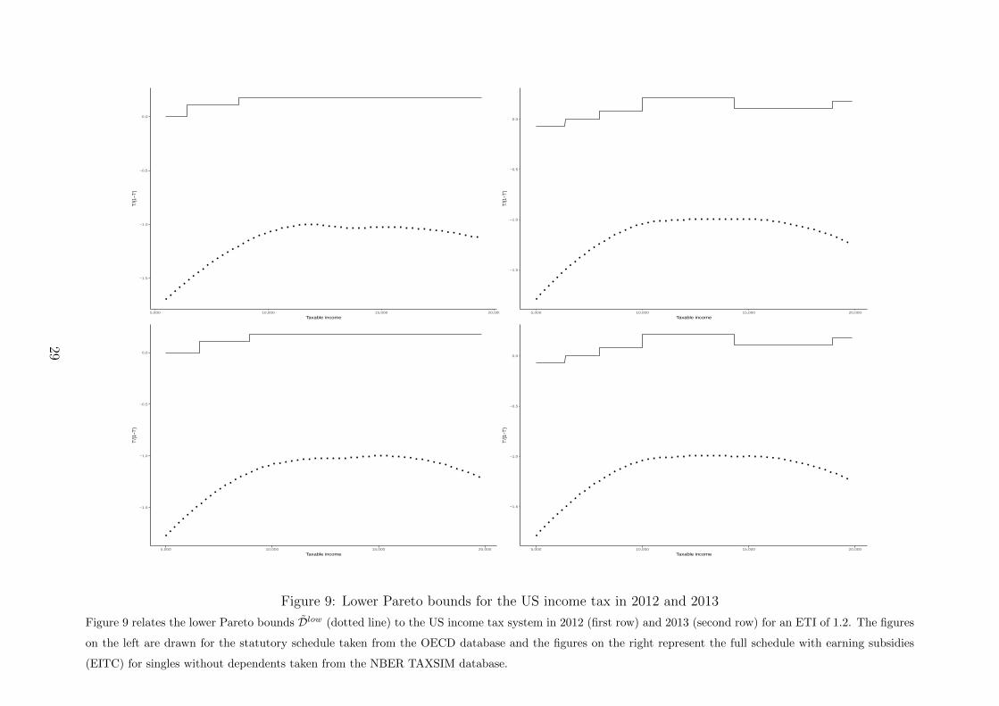
−1.5

−1.0

−0.5

0.0

5,000 10,000 15,000 20,000

Taxable income

T'/(1

−T')

−1.5

−1.0

−0.5

0.0

5,000 10,000 15,000 20,000

Taxable income

T'/(1

−T')

−1.5

−1.0

−0.5

0.0

5,000 10,000 15,000 20,000

Taxable income

T'/(1

−T')

−1.5

−1.0

−0.5

0.0

5,000 10,000 15,000 20,000

Taxable income

T'/(1

−T')

Figure 9: Lower Pareto bounds for the US income tax in 2012 and 2013

Figure 9 relates the lower Pareto bounds Dlow (dotted line) to the US income tax system in 2012 (first row) and 2013 (second row) for an ETI of 1.2. The figures

on the left are drawn for the statutory schedule taken from the OECD database and the figures on the right represent the full schedule with earning subsidies

(EITC) for singles without dependents taken from the NBER TAXSIM database.

29

6.4 Politically feasible reforms

Propositions 5 and 6 characterize Pareto bounds for marginal tax rates. By Theorem 2,

for a status quo such that marginal tax rates are between those bounds, tax increases

for above median incomes and tax cuts for below median incomes are politically feasible.

The following Proposition summarizes these findings.

Proposition 7

1. Let y′ < y0M and T ′0(y′) > Dlow(y′). Then there is a politically feasible reform

(τ, ya, yb) with τ < 0, and ya < y′ < yb.

2. Let y′ > y0M and T ′0(y′) < Dup(y′). Then there is a politically feasible reform

(τ, ya, yb) with τ > 0, and ya < y′ < yb.

According to Proposition 7 political economy forces push for low marginal tax rates

for below median incomes and for high marginal tax rates for above median incomes.

Any attempt to move from the low marginal tax rates to the high marginal tax rates

in a continuous fashion will imply a strong increase of marginal rates for incomes in a

neighborhood of the median. This increase is the price to be paid for having marginal tax

rates close to Dlow for incomes below the median and for having marginal tax rates close to

Dup for incomes above the median. This suggests an explanation for the observation that

some real-world tax schedules are very steep for incomes close to the median.26 Figure

10 presents the tax schedules that are relevant for singles without dependents for the

United States and France in 2012, respectively, taking account of the earnings subsidies

that apply for this group. There is a region where the earnings subsidies are phased out

with the implication of a very pronounced increase of marginal tax rates concentrated in

a narrow range of incomes.27 Moreover, the steep region is, by and large, in the vicinity

of median income. In 2012 the median income for the equal-split distribution is around

18000 euros in France and $24200 in the US (wid.world database).28

6.5 Politically feasible welfare-improvements

We now clarify the relation between politically feasible reforms and welfare-improving

reforms. We are particularly interested in identifying reforms that are both politically

26Germans refer to this as the “Mittelstandsbauch” (middle class belly) in the income tax schedule,

for complementary evidence from the Netherlands see Jacobs et al. (2017).27The earnings subsidies for other groups, such as e.g. single mothers with children, are larger than

those for singles without dependents with the implication that the phase-out region is even steeper for

these groups.28These observations are not sensitive to the notion of median income that is employed. For the

US, median individual income is $21,157 and median household income $50,348 in 2012 (March CPS

database). The numbers are 21679 euros and 16716 euros for France for fiscal households (foyer fiscaux)

and single without dependents, respectively (CASD ERFS database).

30

10000 20000 30000 40000

Taxable income| | | |

-100

00

1000

2000

3000

4000

10000 20000 30000 40000

Taxable income| | | |

-200

00

2000

4000

6000

Figure 10: Income tax schedules for singles without dependants from micro-simulation

models for the US (left figure) and France (right figure) in 2012

Figure 10 is based on the information provided by NBER TAXSIM simulator (accessible on http : //users.nber.org/ taxsim/taxsim9/)

and the TAXIPP simulator (not accessible online, description available on https : //www.ipp.eu/en/tools/taxipp − micro −

simulation/project/).

feasible and welfare-improving.29

Welfare improvements. We begin with a Proposition that clarifies the conditions

under which, for a given specification of welfare weights g, a small tax reform yields an

increase in welfare. The following notation enables us to state the Proposition in a concise

way. We define

γ0 :=

∫ ω

ω

g(ω)u0c(ω)f(ω) dω ,

where u0c(ω) is a shorthand for the marginal utility of consumption that a type ω indi-

vidual realizes under the status quo, and

Γ0(ω′) :=

∫ ω

ω′g(ω)u0

c(ω)f(ω)

1− F (ω′)dω .

Thus, γ0 can be viewed as an average welfare weight in the status quo. It is obtained by

multiplying each type’s exogenous weight g(ω) with the marginal utility of consumption

in the status quo u0c(ω), and then computing a population average. By contrast, Γ0(ω′)

gives the average welfare weight of individuals with types above ω′. Note that γ0 = Γ0(ω)

and that Γ0 is a non-increasing function.

29Our analysis of welfare-improving reforms can also be related to a literature that seeks to identify

society’s social welfare function empirically – see, for instance, Christiansen and Jansen (1978), Blundell,

Brewer, Haan and Shephard (2009), Bourguignon and Spadaro (2012), Bargain, Dolls, Neumann, Peichl

and Siegloch (2011), Hendren (2014), Zoutman, Jacobs and Jongen (2014), Lockwood and Weinzierl

(2016), or Bastani and Lundberg (2017). Through the lens of our model, this literature can alternatively

be interpreted as identifying the set of social welfare functions for which a given reform would be welfare-

improving.

31

Proposition 8 Let

DWg (y) := −1− F (ω0(y))

f(ω0(y))Φ0(ω0(y))

y∗ω(0, 0, ω0(y))

y∗τ (0, 0, ω0(y))

,

where Φ0(ω) := 1− I0(ω)− (1− I0)Γ0(ω)γ0

.

1. Suppose there is an income level y′ so that T ′0(y′) < DWg (y′). Then there exists a

welfare-increasing reform (τ, ya, yb) with τ > 0, and ya < y′ < yb.

2. Suppose there is an income level y′ so that T ′0(y′) > DWg (y′). Then there exists a

welfare-increasing reform (τ, ya, yb) with τ < 0, and ya < y′ < yb.

The corresponding sufficient statistic DWg admits an easy interpretation if there are no

income effects so that the utility function is quasi-linear in private goods consumption and

if the costs of productive effort are iso-elastic. In this case, we have I0 = 0, I0(ω) = 0,

and u0c(ω) = 1 for all ω. This implies, in particular, that γ0 = 1, Γ0(ω) = G(ω) :=∫ ω

ωg(s) f(s)

1−F (ω)ds, and Φ0(ω) = 1−G(ω) , for all ω. Consequently,

DWg (y) =1− F (ω0(y))

f(ω0(y)) ω0(y)

(1−G(ω0(y))

) (1 +

1

ε

),

where the right-hand side of this equation is the ABC-formula due to Diamond (1998).

Politically feasible welfare improvements. Propositions 5 - 8 provide us with a

characterization of the conditions under which a status quo tax policy admits reforms

that are politically feasible or welfare-improving. Looking at the intersection of these

conditions and using the fact that, for all y, Dlow(y) ≤ DWg (y) ≤ Dup(y), yields sufficient

conditions for the existence of reforms that are politically feasible and welfare improving.

The following Proposition states these conditions. A formal proof is omitted.

Proposition 9

1. Let y′ < y0M and T ′0(y′) > DWg (y′). Then there is a politically feasible and welfare-

improving reform (τ, ya, yb) with τ < 0, and ya < y′ < yb.

2. Let y′ > y0M and T ′0(y′) < DWg (y′). Then there is a politically feasible reform

(τ, ya, yb) with τ > 0, and ya < y′ < yb.

For below median incomes, lowering tax rates is politically feasible by Proposition 7. It

is also welfare-improving, if, in the status quo, tax rates exceed DWg . For above median

incomes, raising taxes is politically feasible. This is welfare-improving if tax rates initially

fall short of DWg .

Proposition 9 states sufficient conditions for the existence of welfare-improving and

politically feasible reforms. This raises the question of necessary conditions. Proposition

9 has been derived from focussing on “small” reforms, i.e., on small increases of marginal

32

tax rates applied to a small range of incomes. The arguments in the proofs of Propositions

5 - 8 imply that these conditions are also necessary in the following sense: if either

y′ < y0M and T ′0(y′) ≤ DWg (y′) ,

or

y′ > y0M and T ′0(y′) ≥ DWg (y′) ,

then there is no “small” reform for incomes close to y′ that is both welfare-improving and

politically feasible.30

The analysis suggests that existing tax schedules might be viewed as resulting from

a compromise between concerns for welfare-maximization on the one hand, and concerns

for political support on the other. If the maximization of political support was the only

force in the determination of tax policy, we would expect to see tax rates close to the

revenue-maximizing rate Dup for incomes above the median and negative rates close to

Dlow for incomes below the median. Concerns for welfare dampen these effects. A welfare-

maximizing approach will generally yield higher marginal tax rates for incomes below the

median and lower marginal tax rates for incomes above the median.

Our analysis also raises a question. Diamond (1998) and Saez (2001) have argued

that, for plausible specifications of welfare weights, existing tax schedules have marginal

tax rates for high incomes that are too low. Our analysis suggests that an increase of

these tax rates is not only welfare-improving but also politically feasible. Why don’t we

see more reforms that involve higher tax rates for the rich? Proposition 1 provides a

possible answer to this question: reforms that involve tax cuts that are larger for richer

taxpayers may as well prove to be politically feasible. For such reforms political feasibility

requires that the median voter is included in the set of those who benefit from the tax

cuts.

y < y0M y > y0M

Pareto Political Welfare Pareto Political Welfare

T ′0(y) > Dup(y) ↓ ↓ ↓ ↓ ↓ ↓Dup(y) > T ′0(y) > DWg (y) - ↓ ↓ - ↑ ↓DWg (y) > T ′0(y) > Dlow(y) - ↓ ↑ - ↑ ↑

T ′0(y) < Dlow(y) ↑ ↑ ↑ ↑ ↑ ↑

Table 2: Summary of Propositions 5 - 9.An Arrow pointing upwards (resp. downwards) indicates that raising (resp. lowering) marginal tax

rates for incomes in a neighborhood of y is Pareto-improving, politically feasible, or welfare-improving.

The symbol “-” indicates that changes of marginal tax rates are neither Pareto-improving nor Pareto-

damaging.

30We omit a more formal version of this statement that would require ε-δ-arguments.

33

Table 2 provides a summary of Propositions 5 - 9: according to the first line, if a tax

system is such that the marginal tax rate at income y exceeds the upper Pareto bound,

then lowering marginal tax rates for incomes in a neighborhood of y is Pareto-improving,

welfare-improving, and politically feasible. Analogously, according to the last line, if tax

rates are inefficiently low in the status quo, then increased rates are Pareto-improving,

welfare-improving and politically feasible. The second and third line consider tax reforms

that are not Pareto-improving. For below median incomes, only tax cuts are politically

feasible. If marginal tax rates are too high according to a given welfare function, then

there is scope for a politically feasible welfare-improvement. Otherwise, there is a conflict

between what is politically feasible and what is desirable from a welfare perspective. For

above median incomes, only higher tax rates are politically feasible. Thus, there is scope

for a politically feasible welfare improvement if and only if moving towards higher rates

is also welfare-improving.

7 Extensions

In this section we show that the median voter theorem for small monotonic reforms (The-

orem 1) applies to models with more than one source of heterogeneity among individuals.

Again, we show that a small tax reform is preferred by a majority of taxpayers if and

only if it is preferred by the taxpayer with median income. Throughout, we stick to the

assumption that individuals differ in their productive abilities ω. We introduce a second

consumption good and the possibility of heterogeneity in preferences over consumption

goods in Section 7.1. We use this framework to discuss whether the introduction of dis-

tortionary taxes on savings is politically feasible. In Section 7.2 we consider fixed costs of

labor market participation as an additional source of heterogeneity.31 In Section 7.3 we

assume that individuals differ in their valuation of increased public spending.32 Finally,

in Section 7.4, individuals differ by how much of their income is due to luck as in Alesina

and Angeletos (2005).

7.1 Political support for taxes on savings

We now suppose that there are two consumption goods. We refer to them as food and

savings, respectively. An individual’s budget constraint now reads as

cf + cs + T0s(cs) + τshs(cs) ≤ c0 + y − T0(y)− τh(y) . (9)

The variables on the right-hand side of the budget constraint have been defined before.

On the left-hand side, cf denotes food consumption and cs savings. In the status quo

savings are taxed according to a possibly non-linear savings-tax function T0s. A reform

31See Saez (2002), Chone and Laroque (2011), and Jacquet, Lehmann and Van der Linden (2013).32See Boadway and Keen (1993), Hellwig (2004), Bierbrauer (2014), or Weinzierl (2018).

34

replaces both the status quo income tax schedule T0 by T1 = T0 + τh and the status

quo savings tax schedule T0s by T1s = T0s + τshs. We maintain the assumption that the

functions h and hs are non-decreasing and focus on revenue neutral reforms so that either

τ > 0 and τs < 0 or τ < 0 and τs > 0.

Preferences of individuals are given by a utility function u(v(cf , cs, β), y, ω), where v is

a subutility function that assigns consumption utility to any consumption bundle (cf , cs).

The marginal rate of substitution between food and savings depends on a parameter β.

We do not assume a priori that β is the same for all individuals. Under this assumption,

however, the utility function u has the properties under which an efficient tax system

does not involve distortionary commodity taxes, see Atkinson-Stiglitz (1976), or Laroque

(2005) for a more elementary proof. Distortionary taxes on savings are then undesirable

from a welfare-perspective.

Individuals choose cf , cs and y to maximize utility subject to the budget constraint

above. We denote the utility maximizing choices by c∗f (τs, τ, β, ω), c∗s(τs, τ, β, ω) and

y∗(τs, τ, β, ω) and the corresponding level of indirect utility by V (τs, τ, β, ω). The slope of

an indifference curve in a τ -τs diagram determines the individuals’ willingness to accept

higher savings taxes in return for lower taxes on current earnings. The following Lemma

provides a characterization of this marginal rate of substitution in a neighborhood of the

status quo. Let

s(τ, τ s, β, ω) = − Vτ (τs, τ, β, ω)

Vτs(τs, τ, β, ω)

be the slope of an individual’s indifference curve in a τ -τs diagram. The slope in the

status quo is denoted by s0(ω, β). We denote the individual’s food consumption, savings

and earnings in the status quo by c0f (ω, β), c0

s(ω, β) and y0(ω, β), respectively.

Lemma 4 In the status quo the slope of a type (ω, β)-individual’s indifference curve in

a τ -τs diagram is given by

s0(ω, β) = − h(y0(ω, β))

hs(c0s(ω, β))

.

The proof of Lemma 4 can be found in the Appendix. The Lemma provides a gener-

alization of Roy’s identity that is useful for an analysis of non-linear tax systems. As

is well known, with linear tax systems, the marginal effect of, say, an increased savings

tax on indirect utility is equal to −λ∗c∗s(·), where λ∗ is the multiplier on the individual’s

budget constraint, also referred to as the marginal utility of income. Analogously, the

increase of a linear income tax affects indirect utility via −λ∗y∗(·) so that the slope of an

indifference curve in a τs-τ -diagram would be equal to the earnings-savings-ratio −y∗(·)c∗s(·) .

Allowing for non-linear tax systems and non-linear perturbations implies that the simple

earnings-savings-ratio is replaced by − h(y∗(·))hs(c∗s(·)) .

35

Consider a reform that involves an increase in the savings tax rate dτs > 0 and a

reduction of taxes on income dτ < 0. We say that a type (ω, β)-individual strictly prefers

a small reform with increased savings taxes over the status quo if

Vτs(0, 0, β, ω) dτs + Vτ (0, 0, β, ω) dτ > 0 ,

or, equivalently, if

dτsdτ

> s0(ω, β) = − h(y0(ω, β))

hs(c0s(ω, β))

. (10)

Since hs is an increasing function, this condition is, ceteris paribus, easier to satisfy if the

individual has little savings in the status quo.33

Different types will typically differ in their generalized earnings-savings-ratio s0(ω, β)

and we can order types according to this one-dimensional index. Let (ω, β)0M be the

type with the median value of s0(ω, β). The following proposition extends Theorem 1.

It asserts that a small reform is politically feasible if and only if it is supported by the

median type (ω, β)0M .

Proposition 10 For a given status quo tax policy and a given pair of non-decreasing

functions h and hs, the following statements are equivalent:

1. Type (ω, β)0M prefers a small reform with increased savings taxes over the status

quo.

2. There is a majority of individuals who prefer a small reform with increased savings

taxes over the status quo.

As Theorem 1, Proposition 10 exploits the observation that individuals can be ordered

according to a one-dimensional statistic that pins down whether or not they benefit

from a tax reform. This makes it possible to prove a median-voter theorem for reforms

that remain in a neighborhood of the status quo. There is also an important difference

to Theorem 1. With only one-dimensional heterogeneity, there is a monotonic relation

between types and earnings so that the identity of the type with median income does not

33The ratio dτsdτ on the left-hand side of inequality (10) is determined as follow: Let ∆Rs(τs, τ) be the

change of revenue from savings taxes and ∆R(τs, τ) the change of revenue from income taxation due to

the reform. Revenue-neutrality requires that

∆Rsτs (τs, τ)d τs + ∆Rs

τ (τs, τ) dτ + ∆Rτs(τs, τ) dτs + ∆R

τ (τs, τ) dτ = 0 ,

or, equivalently, that

dτsdτ

= −∆Rτ (τs, τ) + ∆Rs

τ (τs, τ)

∆Rsτs (τs, τ) + ∆R

τs(τs, τ),

which has to be evaluated for (τs, τ) = (0, 0). We assume that this expression is well-defined and takes

a finite negative value.

36

depend on the status quo. Whatever the tax system, the person with the median income

is the person with the median type ωM . Here, by contrast, we allow for heterogeneity

both in productive abilities and in preferences over consumption goods. The type with the

median value of the generalized earnings-savings-ratio s0(ω, β) will then typically depend

on the status quo tax system. This does not pose a problem if we focus on small reforms.

In this case, preferences over reforms follow from the generalized earnings-savings-ratios

in the status quo, and a small reform is preferred by a majority of individuals if and only

if it is preferred by the individual with the median ratio.

7.2 Fixed costs of labor market participation

With fixed costs of labor market participation individuals derive utility u(c−θ 1y>0, y, ω)

from a (c, y)-pair. Fixed costs θ absorb some of the individual’s after-tax income if the

individual becomes active on the labor market, e.g. because of additional child care

expenses. As before, there is an initial status quo tax schedule under which earnings are

transformed into after-tax income according to the schedule C0 with C0(y) = c0+y−T0(y).

After a reform, the schedule is

C1(y) = c0 + ∆R + y − T0(y)− τ h(y) ,

where h is a non-decreasing function of y. We denote by y∗(∆R, τ, ω, θ) the solution to

maxy

u(C1(y)− θ 1y>0, y, ω),

and the corresponding level of indirect utility by V (∆R, τ, ω, θ). We proceed analogously

for other variables: what has been a function of ω in previous sections is now a function

of ω and θ.

For a given function h, the marginal gain that is realized by an individual with type

(ω, θ) if the tax rate τ is increased, is given by the following analogue to equation (4),

∆Vτ (ω, θ | τ, h) = u1

c(ω, θ)(∆Rτ (τ, h)− h(y1(ω, θ))

), (11)

where u1c(ω, θ) is the marginal utility of consumption realized by a type (ω, θ)-individual

after the reform, and y1(ω, θ) are the individual’s post-reform earnings. At τ = 0, we can

also write

∆Vτ (ω, θ | 0, h) = u0

c(ω, θ)(∆Rτ (0, h)− h(y0(ω, θ))

), (12)

where u0c(ω, θ) and y0(ω, θ) are, respectively, marginal utility of consumption and earnings

in the status quo.

For a given status quo tax policy and a given function h we say that type (ω, θ)

strictly prefers a small tax reform over the status quo if ∆Vτ (ω, θ | 0, h) > 0. The

status quo median voter strictly prefers a small reform if ∆Vτ

((ω, θ)0M | 0, h

)> 0, where

y0M is the median of the distribution of earnings in the status quo and (ω, θ)0M is the

corresponding type; i.e. y0((ω, θ)0M

)= y0M .

37

Proposition 11 For a given status quo tax policy and a monotonic function h, the fol-

lowing statements are equivalent:

1. Type (ω, θ)0M prefers a small reform over the status quo.

2. There is a majority of individuals who prefer a small reform over the status quo.

Proposition 11 exploits that the slope of a type (ω, θ) individual’s indifference curve

through a point (τ,∆R),

s(τ,∆R, ω, θ) = h(y∗(∆R, τ, ω, θ)) .

is a function of the individual’s income. As in the basic Mirrleesian setup, the inter-

pretation is that individuals with a higher income are more difficult to convince that a

reform that involves tax increases (τ > 0) is worthwhile. A difference to the Mirrleesian

setup is, however, that there is no monotonic relation between types and earnings. In

the presence of income effects, and for a given level of ω, y∗ will increase in θ as long as

θ is below a threshold θ(ω) and be equal to 0 for θ above the threshold. Moreover, the

threshold is affected by tax policy. This implies that there is no longer a fixed type whose

income is equal to the median income whatever the tax schedule. As in Proposition 10,

this does not pose a problem if we focus on small reforms, i.e. on small deviations from

(τ,∆R) = (0, 0). In this case, preferences over reforms follow from the relation between

types and earnings in the status quo, and a small reform is preferred by a majority of

individuals if and only if it is preferred by the individual with the median level of income

in the status quo.

7.3 Public-goods preferences

Suppose that the change in revenue ∆R is used to increase or decrease spending on

publicly provided goods. The post-reform consumption schedule is then given by

C1(y) = c0 + y − T0(y)− τ h(y) ,

We assume that individuals differ with respect to their public-goods preferences. Now

the parameter θ is a measure of an individual’s willingness to give up private goods con-

sumption in exchange for more public goods. More specifically, we assume that individual

utility is

u(θ(R0 + ∆R) + C1(y), y, ω) ,

where R0 is spending on publicly provided goods in the status quo. Again, we denote by

y∗(∆R, τ, ω, θ) the solution to

maxy

u(θ(R0 + ∆R) + C1(y), y, ω)

38

and indirect utility by V (∆R, τ, ω, θ). By the envelope theorem, the slope of a type (ω, θ)

individual’s indifference curve through point (τ,∆R) is now given by

s(τ,∆R, ω, θ) =h(y∗(∆R, τ, ω, θ))

θ.

This marginal rate of substitution gives the increase in public-goods provision that an

individual requires as a compensation for an increase of marginal tax rates. Ceteris

paribus, individuals with a lower income and individuals with a higher public-goods

preference require less of a compensation, i.e. they have a higher willingness to pay higher

taxes for increased public-goods provision. If we focus on small reforms we observe, again,

that if a type (ω, θ)-individual benefits from a small tax-increase, then the same is true

for any type (ω′, θ′) with

h(y0(ω, θ))

θ≥ h(y0(ω′, θ′))

θ′.

By the arguments in the proof of Proposition 11, a small reform with τ > 0 is preferred

by a majority of individuals if and only if(h(y0(ω, θ))

θ

)0M

< ∆Rτ (0, h) ,

where(h(y0(ω,θ))

θ

)0M

is the median willingness to pay higher taxes for increased public

spending in the status quo.

7.4 Fairness and politically feasible reforms

The validity of our approach does not dependent on the assumption that voting behavior

is driven by narrow self-interest. To illustrate this insight, we analyze politically feasible

reforms in the context of a model in which social preferences determine political support

for redistributive taxation. Specifically, we adopt the framework of Alesina and Angeletos

(2005). Alesina and Angeletos assume that individual incomes can be due to luck or effort

and that preferences over tax policies include a motive to tax income that is due to luck

more heavily than income that is due to effort. Alesina and Angeletos focus, however, on

linear tax systems.

There are two periods. When young individuals choose a level of human capital

k. When old individuals choose productive effort or labor supply l. Pre-tax income is

determined by

y = π(l, k) + η ,

where π is a production function that is increasing in both arguments and η is a random

source of income, also referred to as luck. An individual’s life-time utility is written as

u(c, l, k, ω). Utility is increasing in the first argument. It is decreasing in the second and

third argument to capture the effort costs of labor supply and human capital investments,

39

respectively. Effort costs are decreasing in ω. More formally, lower types have steeper

indifference curves both in a (c, l)-space and in a (c, k)-space. We consider reforms that

lead to a consumption schedule

C1(y) = c0 + ∆R + y − T0(y)− τ h(y) .

We assume that individuals first observe how lucky they are and then choose how hard

they work, i.e. given a realization of η and given the predetermined level of k, individuals

choose l so as to maximize

u(C1(π(l, k) + η), l, k, ω) .

We denote the solution to this problem by l∗(∆R, τ, ω, η, k). Indirect utility is denoted by

V (∆R, τ, ω, η, k). As of t = 1, there is multi-dimensional heterogeneity among individuals:

they differ in their type ω, in their realization of luck η and possibly also in their human

capital k.

In Alesina and Angeletos (2005) preferences over reforms have a selfish and fairness

component. The indirect utility function V shapes the individuals’ selfish preferences over

reforms. The analysis of these selfish preferences can proceed along similar lines as the

extension that considered fixed costs of labor market participation. Selfish preferences

over small reforms follow from the relation between types and earnings in the status

quo, and a small reform makes a majority better off if and only if it is beneficial for

the individual with the median level of income in the status quo. More formally, let

y0(ω, η, k) := y∗(0, 0, ω, η, k) be a shorthand for the earnings of a type (ω, η, k)-individual

in the status quo and recall that the sign of

s(0, 0, ω, η, k) = h(y0(ω, η, k))

determines whether an individual benefits from a small tax reform. Specifically, suppose

that h is a non-decreasing function and denote by y0M the median level of income in

the status quo and by (ω, η, k)0M the corresponding type. A majority of individuals is

– according to their selfish preferences – made better off if and only if the median voter

benefits from the reform,

s0((ω, η, k)0M

)= h

(y0M

)< ∆R

τ (0, h) .

In their formalization of social preferences, Alesina and Angeletos (2005) view π(l, k)

as a reference income. It is the part of income that is due to effort as opposed to luck. A

tax reform affects the share of y = π(l, k) + η that individuals can keep for themselves.

After the reform, the difference between disposable income and the reference income is

given by34

C1(y)− π(l, k) = η − T0(π(l, k) + η)− τh(π(l, k) + η) .

34The analysis in Alesina and Angeletos (2005) looks at a special case of this. They focus on a status

quo equal to the laissez-faire schedule so that T0(y) = 0, for all y, and a reform that introduces a linear tax

schedule, i.e. h(y) = y, for all y. Under these assumptions, we have η−T0(π(l, k)+η)−τh(π(l, k)+η) =

(1− τ)η + τπ(l, k) .

40

A social preferences for fair taxes is then equated with a desire to minimize the variance

of η − T0(π(l, k) + η) − τh(π(l, k) + η) taking into account that k and l are endogenous

variables.35 Denote this variance henceforth by Σ(∆R, τ). Any one individual is assumed

to evaluate a tax reform according to

V (∆R, τ, ω, η, k)− ρ Σ(∆R, τ) ,

where ρ is the weight on fairness considerations which is assumed to be the same for

all individuals. Therefore, heterogeneity in preferences over reforms is entirely due to

heterogeneity in selfish preferences. Consequently, the finding that a small reform is

preferred by a majority of taxpayers if and only if it is preferred by the voter with

median income in the status quo is not affected by the inclusion of a demand for fair

taxes.

8 Concluding remarks

This paper develops a framework for a political economy analysis of tax reforms. With

non-linear tax systems, the policy-space is multi-dimensional with the implication that

political economy forces are difficult to characterize. One of our main results is that this

difficulty can be overcome by looking at tax reforms such that the change in tax payments

is a monotonic function of income. We show that, with such a policy space, a reform is

preferred by a majority of taxpayers if and only if it is preferred by the taxpayer with

median income. This implies that tax decreases for incomes below the median and tax

increases for incomes above the median are politically feasible.

Our analysis identifies, for each level of income, Pareto-bounds for marginal tax rates.

It also identifies reforms that would be preferred by a majority of voters. Moreover, we

derive sufficient statistics that make it possible to bring this framework to the data. This

enables us to diagnose what types of reforms are possible under a given status quo tax

policy. Future research might use this framework to complement existing studies on the

history of income taxation. For instance, Scheve and Stasavage (2016) study whether

tax systems have become more progressive in response to increases in inequality or in

response to extensions of the franchise. Their analysis compares tax policies that have

been adopted at different points in time, or by countries with different institutions. It

does not include an analysis of the reforms that appear to have been politically feasible or

welfare-improving in a given year for a given country and a given status quo tax schedule.

The framework that is developed in this paper lends itself to such an analysis.

We develop the main argument in the context of a classical Mirrleesian model of in-

come taxation. We also show that our analysis of small monotonic reforms extends to

35Human capital investment is a function of effort costs ω and the expectations (∆Re, τe) of the young

on the tax reforms that will be adopted when they are old.

41

models with multi-dimensional heterogeneity of individuals, such as models with vari-

able and fixed costs of labor market participation, models that include heterogeneity in

preferences over public goods, or models that include an investment in human capital.

The focus on monotonic reforms has enabled us to prove a median voter theorem for

non-linear tax systems. Moreover, the use of the perturbation method made it possible

to identify directions for politically feasible reforms by means of sufficient statistics. The

logic of this argument is not tied to non-linear tax systems and we conjecture that a

similar analysis is possible for other multi-dimensional policy domains. What is needed,

however, is that a focus on monotonic reforms is justified. For taxation, monotonicity

holds provided that tax cuts or increases are monotonic functions of income – a property

that is satisfied by most reforms in actual tax policy.

References

Acemoglu, D., M. Golosov, and A. Tsyvinski, “Political Economy of Mechanisms,”

Econometrica, 2008, 76, 619–641.

, , and , “Dynamic Mirrlees Taxation under Political Economy Con-

straints,” Review of Economic Studies, 2010, 77, 841–881.

, S. Naidu, P. Restrepo, and J.A. Robinson, “Democracy, Redistribution, and

Inequality,” Handbook of Income Distribution, 2015, pp. 1885–1966.

Adam, S., J. Browne, D. Phillips, and B. Roantree, “Frictions and taxpayer

responses: evidence from bunching at personal tax thresholds,” Working paper In-

stitute for Fiscal Studies, 2017.

Alesina, A. and G.-M. Angeletos, “Fairness and Redistribution,” American Eco-

nomic Review, 2005, 95 (4), 960–980.

, S. Stantcheva, and E. Teso, “Intergenerational Mobility and Support for Re-

distribution,” American Economic Review, 2018, 108 (2), 521–554.

Alvaredo, F., A.B. Atkinson, L. Chancel, T. Piketty, E. Saez, and G. Zucman,

“Distributional National Accounts (DINA) Guidelines: Concepts and Methods used

in WID.world,” WID.world Working Paper Series, 2016.

Atkinson, A. and J. Stiglitz, “The Design of Tax Structure: Direct versus Indirect

Taxation,” Journal of Public Economics, 1976, 1, 55–75.

Bargain, O., M. Dolls, D. Neumann, A. Peichl, and S. Siegloch, “Tax-Benefit

Systems in Europe and the US: Between Equity and Efficiency,” IZA Discussion

Papers 5440, 2011.

42

Barro, R.J., “The Control of Politicians: An economic model,” Public Choice, 1973, 14,

19–42.

Bastani, S. and J. Lundberg, “Political preferences for redistribution in Sweden,”

Journal of Economic Inequality, 2017, 15 (4), 345–367.

Benabou, R., “Unequal Societies: Income Distribution and the Social Contract,” Amer-

ican Economic Review, 2000, 90 (1), 96–129.

Benabou, R. and E.A. Ok, “Social Mobility and the Demand for Redistribution: The

Poum Hypothesis,” Quarterly Journal of Economics, 2001, 116 (2), 447–487.

and J. Tirole, “Belief in a just world and redistributive politics,” Quarterly Journal

of Economics, 2006, 121 (2), 699–746.

Besley, T. and S. Coate, “A Model of Representative Democracy,” Quarterly Journal

of Economics, 1997, 112, 85–114.

Bierbrauer, F.J., “Optimal Tax and Expenditure Policy with Aggregate Uncertainty,”

American Economic Journal: Microeconomics, 2014, 6 (1), 205–57.

and P.C. Boyer, “Efficiency, Welfare, and Political Competition,” Quarterly Jour-

nal of Economics, 2016, 131 (1), 461–518.

Black, D., “On the Rationale of Group Decision-making,” Journal of Political Economy,

1948, 56 (1), 23–34.

Blanchet, T., J. Fournier, and T. Piketty, “Generalized Pareto Curves: Theory and

Applications,” WID.world Working Paper Series,, 2017.

Blomquist, S. and W. Newey, “The Bunching Estimator Cannot Identify the Taxable

Income Elasticity,” NBER Working Paper 24136, 2017.

Blundell, R., M. Brewer, P. Haan, and A. Shephard, “Optimal income taxation of

lone mothers: an empirical comparison of the UK and Germany,” Economic Journal,

2009, 119, F101–F121.

Boadway, R. and M. Keen, “Public Goods, Self-Selection and Optimal Income Tax-

ation,” International Economic Review, 1993, 34, 463–478.

Bohn, H. and C. Stuart, “Revenue Extraction by Median Voters,” Working Paper,

University of California at Santa Barbara 2013.

Bourguignon, F. and A. Spadaro, “Tax-benefit Revealed Social Preferences,” Journal

of Economic Inequality, 2012, 10 (1), 75–108.

43

Brett, C. and J.A. Weymark, “Voting over selfishly optimal nonlinear income tax

schedules with a minimum-utility constraint,” Journal of Mathematical Economics,

2016, 67, 18–31.

and , “Voting over selfishly optimal nonlinear income tax schedules,” Games

and Economic Behavior, 2017, 101, 172–188.

Cabannes, P.-Y., C. Houdre, and C. Landais, “Comment le revenu imposable des

menages reagit-il a sa taxation? Une estimation sur la periode 1997-2004,” Economie

et statistique, 2014, 467 (1), 141–162.

Chetty, R., “Sufficient Statistics for Welfare Analysis: A Bridge Between Structural

and Reduced-Form Methods,” Annual Review of Economics, 2009, 1 (1), 451–488.

Chone, P. and G. Laroque, “Optimal taxation in the extensive model,” Journal of

Economic Theory, 2011, 146 (2), 425–453.

Christiansen, V. and E. Jansen, “Implicit Social Preferences in the Norwegian System

of Indirect Taxation,” Journal of Public Economics, 1978, 10 (2), 217–245.

Diamond, P.A., “Optimal Income Taxation: An Example with a U-Shaped Pattern of

Optimal Marginal Tax Rates,” American Economic Review, 1998, 88, 83–95.

Farhi, E., C. Sleet, I. Werning, and S. Yeltekin, “Non-linear Capital Taxation

Without Commitment,” Review of Economic Studies, 2012, 79 (4), 1469–1493.

Feldstein, M., “On the theory of tax reform,” Journal of Public Economics, 1976, 6

(1-2), 77–104.

Ferejohn, J., “Incumbent Performance and Electoral Control,” Public Choice, 1986, 50,

5–25.

Gans, J.S. and M. Smart, “Majority voting with single-crossing preferences,” Journal

of Public Economics, 1996, 59 (2), 219 – 237.

Golosov, M., A. Tsyvinski, and N. Werquin, “A Variational Approach to the

Analysis of Tax Systems,” NBER Working Paper 20780, 2014.

Guesnerie, R., A Contribution to the Pure Theory of Taxation, Cambridge University

Press, 1995.

Heathcote, J., K. Storesletten, and G.L. Violante, “Optimal Tax Progressivity:

An Analytical Framework,” Quarterly Journal of Economics, 2017, 132 (4), 1693–

1754.

44

Hellwig, M.F., “Optimal income taxation, public-goods provision and public-sector

pricing: A contribution to the foundations of public economics,” MPI Collective

Goods Preprint, 2004, 2004/14.

Hendren, N., “The Inequality Deflator: Interpersonal Comparisons without a Social

Welfare Function,” NBER Working Paper 20351, 2014.

Jacobs, B., E.L.W. Jongen, and F.T. Zoutman, “Revealed social preferences of

Dutch political parties,” Journal of Public Economics, 2017, 156, 81–100.

Jacquet, L. and E. Lehmann, “Optimal Taxation with Heterogeneous Skills and Elas-

ticities: Structural and Sufficient Statistics Approaches,” THEMA Working Paper

2016/04, 2016.

, , and B. Van der Linden, “Optimal redistributive taxation with both

extensive and intensive responses,” Journal of Economic Theory, 2013, 148 (5),

1770 – 1805.

Kleven, H.J., “Bunching,” Annual Review of Economics, 2016, 8, 435–464.

, “Sufficient Statistics Revisited,” Mimeo Princeton, 2018, pp. 1–30.

Laroque, G., “Indirect taxation is superfluous under separability and taste homogeneity:

a simple proof,” Economic Letters, 2005, 87, 141–144.

Lockwood, B.B. and M. Weinzierl, “Positive and normative judgments implicit in

U.S. tax policy, and the costs of unequal growth and recessions,” Journal of Monetary

Economics, 2016, 14-119 (77), 30–47.

Lorenz, N. and D. Sachs, “Identifying Laffer Bounds: A Sufficient-Statistics Approach

with an Application to Germany,” Scandinavian Journal of Economics, 2016, 118

(4), 646–665.

Meltzer, A. and S. Richard, “A Rational Theory of the Size of Government,” Journal

of Political Economy, 1981, 89, 914–927.

Mertens, K. and J.L.M. Olea, “Marginal Tax Rates and Income: New Time Series

Evidence,” Quarterly Journal of Economics, 2018.

Mirrlees, J., “An Exploration in the Theory of Optimum Income Taxation,” Review of

Economic Studies, 1971, 38, 175–208.

Osborne, M. and A. Slivinski, “A Model of Political Competition With Citizen-

Candidates,” Quarterly Journal of Economics, 1996, 111, 65–96.

Piketty, T., “Social mobility and redistributive politics,” Quarterly Journal of Eco-

nomics, 1995, 110 (3), 551–584.

45

, “La redistribution fiscale face au chomage,” Revue francaise d’economie, 1997, 12,

157–201.

Roell, A.A., “Voting over Nonlinear Income Tax Schedules,” Working Paper, 2012.

Roberts, K., “Voting over Income Tax Schedules,” Journal of Public Economics, 1977,

8.

Rothstein, P., “Order restricted preferences and majority rule,” Social Choice and

Welfare, 1990, 7 (4), 331–342.

, “Representative Voter Theorems,” Public Choice, 1991, 72 (2/3), 193–212.

Saez, E., “Using Elasticities to Derive Optimal Income Tax Rates,” Review of Economic

Studies, 2001, 68, 205–229.

, “Optimal Income Transfer Programs: Intensive versus Extensive Labor Supply

Responses,” Quarterly Journal of Economics, 2002, 117 (3), 1039–1073.

, “Do Taxpayers Bunch at Kink Points?,” American Economic Journal: Economic

Policy, August 2010, 2 (3), 180–212.

, “Taxing the rich more: Preliminary evidence from the 2013 Tax Increase,” Tax

Policy and the Economy, 2017, 31 (1), 71–120.

and S. Stantcheva, “Generalized Social Marginal Welfare Weights for Optimal

Tax Theory,” American Economic Review, 2016, 106 (1), 24–45.

, J. Slemrod, and S.H. Giertz, “The elasticity of taxable income with respect

to marginal tax rates: A critical review,” Journal of Economic Literature, 2012, 50

(1), 3–50.

Scheuer, F. and A. Wolitzky, “Capital taxation under political constraints,” Ameri-

can Economic Review, 2016, 106 (8), 2304–2328.

Scheve, K. and D. Stasavage, Taxing the Rich: A History of Fiscal Fairness in the

United States and Europe, Princeton University Press, 2016.

Seade, J., “On the Sign of the Optimum Marginal Income Tax,” Review of Economic

Studies, 1982, 49 (4), 637–643.

Sheshinski, E., “The Optimal Linear Income-tax,” Review of Economic Studies, 1972,

39, 297–302.

Weinzierl, M., “Revisiting the classical view of benefit-based taxation,” Economic Jour-

nal, 2018.

46

Werning, I., “Pareto Efficent Income Taxation,” Mimeo, Massachusetts Institute of

Technology 2007.

Weymark, J.A., “Undominated directions of tax reform,” Journal of Public Economics,

1981, 16 (3), 343–369.

Zoutman, F.T., B. Jacobs, and E.L.W. Jongen, “Optimal Redistributive Taxes and

Redistributive Preferences in the Netherlands,” Working paper Erasmus University

Rotterdam/CPB Netherlands Bureau for Economic Policy Research, 2014.

47

Appendix

A Behavioral responses to simple reforms

A simple reform (τ, ya, yb)-class involves jumps of marginal tax rates at ya and yb. Lemmas

A.1-A.3 below clarify the behavioral responses to these discontinuities. Figure 11 provides an

illustration.

y

c

C1(y)

C0(y)

c0 + ∆R

c0

c0 + ∆R − τ(yb − ya)

ya yb

IC1a

IC2a

IC0a

IC1b

IC2b

IC0b

Figure 11:The figure depicts the following curves:

(a) C0(y) = c0 + y − T0(y), C1(y) = c0 + ∆R

+ y − T0(y)− τh(y),

(b) IC0b indifference curve of type ωb(0) through yb under C0(y), IC1

b curve through yb under C1(y) when there are no income effects, IC2b

curve through yb under C1(y) with income effects;

(c) IC0a indifference curve of type ωa(0) through ya under C0(y), IC1

a curve through ya under C1(y) when there are no income effects,

IC2a curve through ya under C1(y) if there are income effects.

The Spence-Mirrlees single crossing property implies that, under any tax schedule, more

productive individuals choose a higher level of pre-tax income. Thus, ω′ > ω implies that

y∗(∆R(τ ′, ya, yb), τ′, ω′) ≥ y∗(∆R(τ ′, ya, yb), τ

′, ω) ,

for τ ′ ∈ 0, τ. We can therefore define threshold types ωa(τ′) and ωb(τ

′) so that

ω < ωa(τ′) implies y∗(∆R(τ ′, ya, yb), τ

′, ω) ≤ ya ,

ω ∈ (ωa(τ′), ωb(τ

′)) implies y∗(∆R(τ ′, ya, yb), τ′, ω) ∈ (ya, yb) ,

48

and

ω > ωb(τ′) implies y∗(∆R(τ ′, ya, yb), τ

′, ω) ≥ yb .

The following Lemma asserts that, for a reform that involves an increase of the marginal

tax rate, τ > 0, type ωa(0) who chooses an income of ya before the reform does not choose a

level of income above ya after the reform. Analogously, if marginal taxes go down, type ωb(0)

does not choose an income above yb after the reform. For a reform with τ > 0, the logic is as

follows: After the reform, because of the transfer ∆R, a type ωa(0)-individual is, at income level

ya, less eager to work more. Working more also is less attractive after the reform because of the

increased marginal tax rates for incomes above ya. Thus, both the income and the substitution

effect associated with the reform make it less attractive for a type ωa(0)-individual to increase

her income above ya. The individual will therefore either stay at ya or decrease her income after

the reform. Only higher types will end up with an income of ya after the reform, which implies

ωa(0) ≤ ωa(τ).

Lemma A.1

1. Consider a reform so that τ > 0 and ∆R(τ, ya, yb) > 0. Then ωa(τ) ≥ ωa(0).

2. Consider a reform so that τ < 0 and ∆R(τ, ya, yb) < 0. Then ωb(τ) ≥ ωb(0).

Proof We only prove the first statement. The proof of the second statement follows from an

analogous argument. Under the initial tax schedule T0 an individual with type ωa(0) prefers

ya over all income levels y ≥ ya. We argue that the same is true under the new tax schedule

T1. This proves that ωa(τ) ≥ ωa(0). Consider a y-c-diagram and the indifference curve of

a type wa(0)-type through the point (ya, c0 + ya − T0(ya)). By definition of type wa(0), all

points (y, y−T0(y)) with y > ya lie below this indifference curve under the initial tax schedule.

Under the new schedule T1, this individual receives a lump-sum transfer ∆R > 0. Hence, the

indifference curve through (ya, c0 + ∆R + ya − T0(ya)) is at least as steep as the indifference

curve through (ya, c0 + ya − T0(ya)). Thus, the individual prefers (ya, c0 + ∆R + ya − T0(ya))

over all points (y, c0 + ∆R + y − T0(y)) with y > ya. Since for all y > ya, T1(y) > T0(y), the

individual also prefers (ya, c0 + ∆R + ya − T0(ya)) over all points (y, c0 + ∆R + y − T1(y)) with

y > ya.

According to the next lemma a reform induces bunching of individuals who face an upward

jump of marginal tax rates after the reform. Specifically, a reform with τ > 0 will induce

bunching at ya because marginal tax rates jump upwards at income level ya. A reform with

τ < 0 will induce bunching at yb because marginal tax rates jump upwards at income level yb.

Lemma A.2

1. Consider a reform so that τ > 0 and ∆R(τ, ya, yb) > 0. Then there is a set of types

[ωa(τ), ωa(τ)] who bunch at ya after the reform.

2. Consider a reform so that τ < 0 and ∆R(τ, ya, yb) < 0. Then there is a set of types

[ωb(τ), ωb(τ)] who bunch at yb after the reform.

49

Proof Consider a reform that involves an increase of marginal tax rates τ > 0. If before the

reform, all types were choosing an income level y∗(0, 0, ω) that satisfies the first order condition

uc(·)(1− T ′0(·)) + uy(·) = 0 ,

then, after the reform there will be a set of types (ωa(τ), ω(τ)] who will now bunch at ya. These

individuals chose an income level above ya before the reform. After the reform they will find

that

uc(·)(1− T ′0(·)− τ) + uy(·) < 0 ,

for all y ∈ (ya, y∗(0, 0, ω)] and therefore prefer ya over any income in this range. At the same

time, they will find that

uc(·)(1− T ′0(·)) + uy(·) > 0 ,

so that there is also no incentive to choose an income level lower than ya. Hence, the types who

bunch are those for which at ya,

1− T ′0(ya) > −uy(·)uc(·)

> 1− T ′0(ya)− τ .

An analogous argument implies that for a reform that involves a decrease in marginal tax rates,

τ < 0, there will be a set of types [ωb(τ), ωb(τ)] who bunch at yb after the reform.

Individuals who bunch at ya after a reform with τ > 0 neither have an incentive to increase

their earnings above ya since

uc(·)(1− T ′1(ya)) + uy(·) = uc(·)(1− T ′0(ya)− τ) + uy(·) ≤ 0

nor an incentive to lower their earnings since

uc(·)(1− T ′0(ya)) + uy(·) ≥ 0 .

By contrast, there are no individuals who bunch at yb after a reform that involves increased

marginal tax rates. Individuals who do not have an incentive to increase their income at yb

since

uc(·)(1− T ′1(yb)) + uy(·) = uc(·)(1− T ′0(yb)) + uy(·) ≤ 0

definitely have an incentive to lower their income as

uc(·)(1− T ′0(yb)− τ) + uy(·) < 0 .

An analogous argument implies that no one will bunch at ya after a reform that involves a

decrease of marginal tax rates.

The next Lemma establishes that, in the absence of income effects, for a reform with τ > 0,

individuals who choose an income above yb after the reform also chose an income above yb before

the reform. We will subsequently discuss why these statements need no longer be true if there

are income effects.

50

Lemma A.3 Suppose that there are no income effects, i.e. for all (c, y, ω) and any pair (e, e′)

with e′ > e,

−uy(c+ e, y, ω)

uc(c+ e, y, ω)= −uy(c+ e′, y, ω)

uc(c+ e′, y, ω).

1. Consider a reform so that τ > 0 and ∆R(τ, ya, yb) > 0. Then ωb(τ) ≥ ωb(0).

2. Consider a reform so that τ < 0 and ∆R(τ, ya, yb) < 0. Then ωa(τ) ≥ ωa(0).

Proof We only prove the first statement. The proof of the second statement follows from an

analogous argument. Under the initial tax schedule T0 an individual with type ωb(0) prefers

yb over all income levels y ≥ yb. We argue that the same is true under the new tax schedule

T1. This proves that ωb(τ) ≥ ωb(0). Consider a y-c-diagram and the indifference curve of a

type wb(0)-type through the point (yb, c0 + yb − T0(yb)). By definition of type wb(0), all points

(y, c0 + y − T0(y)) with y > yb lie below this indifference curve under the initial tax schedule.

Under the new schedule T1, this individual receives a lump-sum transfer ∆R − τ(yb − ya) < 0.

Without income effects, the indifference curve through (yb, c0 + ∆R − τ(yb − ya) + yb − T0(yb))

has the same slope as the indifference curve through (yb, c0 + yb− T0(yb)). Thus, the individual

prefers (yb, c0 +∆R−τ(yb−ya)+yb−T0(yb)) over all points (y, c0 +∆R−τ(yb−ya)+y−T0(y))

with y > yb, or equivalently over all points (y, c0 + ∆R + y − T1(y)) with y > yb.

If there are no income effects, then, after a reform with τ > 0, an individual with type ωb(0)

prefers an income level of yb over any income above yb before and after the reform since (i) the

indifference curve through (c0 + yb − T0(yb), yb) has the same slope as the indifference curve

through (c0 + ∆R + yb − T1(yb), yb) and (ii) for y > yb, T′0(y) = T ′1(y) so that the incentives to

increase income above yb are unaffected by the reform. The individual has, however, an incentive

to lower y since, because of the increased marginal tax rate, working less has become cheaper;

i.e. it is no longer associated with as big a reduction of consumption. Thus, ωb(0) ≤ ωb(τ) if

there are no income effects. Figure 11 provides an illustration. With income effects there is

also an opposing force since the individual also has to pay additional taxes τ(yb − ya) − ∆R

which tends to flatten the indifference curve through yb. Thus, there may both be income levels

below yb and income levels above yb that the individual prefers over yb. If the indifference curve

flattens a lot, the individual will end up choosing y > yb after the reform which implies that

ωb(τ) < ωb(0).

A reform (τ, ya, yb) with τ > 0 may yield to a discontinuity in the earnings function

y∗(∆R, τ, ·) at ωb(τ) = supω | y ∗ (∆R, τ, ω) ≤ yb, see Figure 12 below for an illustration.

The reform leads to a kink in the C1-schedule at yb. Depending on the shape of indifference

curves, this may imply that

limω ↑ ωb(τ)

y∗(∆R(τ, ya, yb), τ, ω) < limω ↓ ωb(τ)

y∗(∆R(τ, ya, yb), τ, ω) .

Analogously, a reform (τ, ya, yb) with τ < 0 may come with a discontinuity in the earnings

function y∗(∆R, τ, ·) at ωa(τ).

51

yb

ICb

c

y

Figure 12: The possibility of a hole at yb

The figure illustrates a reform (τ, ya, yb) with τ > 0 and a situation in which type ωb(τ) is indifferent between an income level below yb and an

income level above yb. Consequently, individuals with a type below ωb(τ) choose an income strictly smaller than yb and individuals with a type

above choose an income strictly larger than yb. The earnings function y∗(∆R, τ, ·) therefore exhibits a discontinuity at ωb(τ) and the income

distribution therefore has zero mass in a neighborhood of yb.

B Proofs

Proof of Theorem 1

Step 1. We show that

∆Vτ (ω | 0, h) = u0

c(ω)(∆Rτ (0, h)− h(y0(ω))

),

for all ω ∈ Ω, where u0c(ω) is a shorthand for the marginal utility of consumption that a type

ω-individual realizes in the status quo.

For individuals whose behavior is characterized by a first-order condition, this follows from

a straightforward application of the envelope theorem. If we consider reforms in the (τ, ya, yb)-

class we have to take account of the possibility of bunching. Consider the case with τ > 0. The

case τ < 0 is analogous. With τ > 0, there will be individuals who bunch at ya. For these

individuals, marginal changes of ∆R and τ do not trigger an adjustment of the chosen level of

earnings. Hence,

∆Vτ (ω | τ, h) = d

dτ u(c0 + ∆R(τ, h) + ya − T0(ya)− τh(ya), ya, ω)

= uc(c0 + ∆R(τ, h) + ya − T0(ya)− τh(ya), ya, ω)(∆Rτ (τ, h)− h(ya)

)By assumption, the status quo tax schedule does not induce bunching. Thus, at τ = 0, this

expression applies only to type ωa with y0(ωa) = ya. This proves that

∆Vτ (ω | 0, h) = u0

c(ω)(∆Rτ (0, h)− h(y0(ω))

),

holds for all ω.

Step 2. Suppose that h is a non-decreasing function. An analogous argument applies if h

is non-increasing. We show that ∆Vτ

(ωM | 0, h

)> 0 implies ∆V

τ (ω | 0, h) > 0 for a majority of

individuals. By Step 1, ∆Vτ

(ωM | 0, h

)> 0 holds if and only if ∆R

τ (0, h)−h(y0(ωM )) > 0. As h

52

and y are non-decreasing functions, this implies ∆Rτ (0, h) − h(y0(ω)) > 0, for all ω ≤ ωM , and

hence ∆Vτ (ω | 0, h) > 0 for all ω ≤ ωM .

Step 3. Suppose that h is a non-decreasing function. An analogous argument applies if h

is non-increasing. We show that ∆Vτ

(ωM | 0, h

)≤ 0 implies ∆V

τ (ω | 0, h) ≤ 0 for a majority of

individuals. By Step 1, ∆Vτ

(ωM | 0, h

)≤ 0 holds if and only if ∆R

τ (0, h)−h(y0(ωM )) ≤ 0. As h

and y are non-decreasing functions, this implies ∆Rτ (0, h) − h(y0(ω)) ≤ 0, for all ω ≥ ωM , and

hence ∆Vτ (ω | 0, h) ≤ 0 for all ω ≥ ωM .

Proof of Lemma 1

For individuals whose behavior is characterized by a first-order condition, the utility realized

under a reform that involves a change in the lump-sum-transfer by ∆R and a change of marginal

taxes by τ is given by V (∆R, τ, ω). The marginal rate of substitution between τ and ∆R is

therefore given by(d∆R

dτ

)|dV=0

= −Vτ (∆R, τ, ω)

Ve(∆R, τ, ω).

By the envelope theorem,

Vτ (∆R, τ, ω) = −uc(·) h(y∗(∆R, τ, ω)) and Ve(∆R, τ, ω) = uc(·) .

Thus,(d∆R

dτ

)|dV=0

= h(y∗(∆R, τ, ω)) .

If we consider reforms in the (τ, ya, yb)-class we have to take account of the possibility of

bunching. We only consider the case with τ > 0. The case τ < 0 is analogous. With τ > 0,

there will be individuals who bunch at ya. For these individuals, marginal changes of ∆R and

τ do not trigger an adjustment of the chosen level of earnings. Hence, a marginal change of ∆R

yields a change in utility equal to uc(·). The change in utility due to a change in the marginal

tax rate is given by −uc(·) h(ya) = 0. Again, the marginal rate of substitution equals h(ya) = 0.

Proof of Proposition 1

From Step 1 in the proof of Theorem 1 we know that

∆Vτ (ω | 0, h) = u0

c(ω)(∆Rτ (0, h)− h(y0(ω))

).

To proof the first statement in the Proposition, let

∆Vτ (ωM | 0, h) = u0

c(ωM )(∆Rτ (0, h)− h(y0(ωM ))

)< 0 ,

so that the median voter benfits from a small tax cut, i.e. a small reduction of τ .

With h non-decreasing for y ≥ y0M , this implies that

∆Vτ (ω | 0, h) = u0

c(ω)(∆Rτ (0, h)− h(y0(ω))

)< 0 ,

for all ω ≥ ωM . Hence a majority of the population benefits from the tax cut.

The second statement in the Proposition follows from the same argument: If the poorest

individual benefits from a tax cut and indviduals with incomes closer to the median also benefit

as h is non-decreasing for below median incomes, then there is majority support for the reform.

53

Proof of Lemma 2

We seek to show that, for all ω,

∆Vτ (ω | τ, h) = u1

c(ω)(∆Rτ (τ, h)− h(y1(ω))

).

Suppose that τ > 0. The case τ < 0 is analogous. We first consider reforms (τ, h) under

which individual earnings are characterized by a first order condition. In this case, the envelope

theorem implies

∆Vτ (ω | τ, h) = uc (·)

(∆Rτ (τ, h)− h(y1(ω))

),

where uc(·) is marginal utility evaluated at c = c0 + ∆R(τ, h) + y1(ω)− T1(y1(ω)) and y1(ω) =

y∗(∆R(τ, h), τ, ω).

We now consider a reform that belongs to the (τ, ya, yb)-class. The above reasoning extends

to types with ω ≤ ωa(τ), ω ∈ [ωa(τ), ωb(τ)] and ω ≥ ωb(τ) whose behavior is characterized by

a first order condition. Individuals with types in [ωa(τ), ωa(τ)] bunch at income level ya after

the reform so that

∆V (ω | τ, ya, yb) = u(c0 + ∆R(τ, ya, yb) + ya − T0(ya), ya, ω)− V (0, 0, ω) .

Hence,

∆Vτ (ω | τ, ya, yb) = uc (·) ∆R

τ (τ, ya, yb) ,

where uc(·) is marginal utility evaluated at c = c0 + ∆R(τ, ya, yb) + y− T0(y) and y = ya. Since

h(ya) = 0, this implies, in particular,

∆Vτ (ω | τ, ya, yb) = uc (·)

(∆Rτ (τ, ya, yb)− h(ya)

).

Proof of Proposition 3

Suppose that h is a non-decreasing function. The proof for h non-increasing is analogous. By

(4),

∆Vτ (ωM | τ ′, h) > 0

for all τ ′ ∈ (0, τ), implies

∆Rτ (τ ′, h)− h(y1(ωM )) > 0,

for all τ ′ ∈ (0, τ). By the Spence-Mirrlees single crossing property y1 is a non-decreasing

function. Hence, ω ≤ ωM implies

∆Rτ (τ ′, h)− h(y1(ω)) > 0,

for all τ ′ ∈ (0, τ) and, therefore, by (3) and (4)

∆V (ω | τ ′, h) > 0 ,

again, for all τ ′ ∈ (0, τ). Thus, the reform is supported by a majority of the population. This

proves the first statement in Proposition 3. The second statement follows from an analogous

argument.

54

Proof of Lemma 3

We show that, for all ω,

u1′c (ω) :=

∂

∂ωu1c(ω) ≤ 0 .

Define

y1′(ω) :=∂

∂ωy1(ω) .

By the Spence-Mirrlees single crossing property, y1 is a non-decreasing function: y1′(ω) ≥ 0 for

all ω. Recall that, by definition,

u1c(ω) = uc(c0 + ∆R + y1(ω)− T1(y1(ω)), y1(ω), ω) .

Hence,

u1′c (ω) =

(ucc(·)(1− T ′1(·)) + ucy(·)

)y1′(ω) + ucω(·) .

If the individual is bunching, then y1′(ω) = 0, which implies

u1′c (ω) = ucω(·) ≤ 0 .

It remains to be shown that u1′c (ω) ≤ 0 also holds if the individual is not bunching. If the

individual is not bunching, y1(ω) satisfies the first order condition

1− T ′1(·) = −uy(·)uc(·)

.

Hence,

u1′c (ω) =

(−ucc(·)

uy(·)uc(·)

+ ucy(·))y1′(ω) + ucω(·) ,

where, because of (1),

−ucc(·)uy(·)uc(·)

+ ucy(·) ≤ 0 .

To see this, note that we can also express condition (1) as the requirement that, for any com-

bination of c, y, e and ω, the derivative of −uy(c+e,y,ω)uc(c+e,y,ω) with respect to e is non-negative. This

yields the inequality above.

Proof of Theorem 2

For a small reform in the (τ, ya, yb)-class, evaluated at the status quo, equation (4) implies that

∆Vτ (ω | 0, ya, yb) = u0

c(ω)(∆Rτ (0, ya, yb)− h(y0(ω))

), (13)

To prove the first statement in Theorem 2, suppose that y0 < y0(wM ). Choose ya and yb so that

ya < y0 < yb < y0(wM ). For a reform in the (τ, ya, yb)-class, yb < y0(wM ) implies h(y0(ω)) =

yb − ya, for all ω ≥ ωM . Since ∆Rτ (0, ya, yb) < yb − ya, it follows that ∆V

τ (ω | 0, ya, yb) < 0, for

all ω ≥ ωM , which implies that a small tax cut makes a majority of individuals better off.

To prove the second statement, suppose that y0 > y0(wM ) and choose ya and yb so that

y0(wM ) < ya < y0 < yb. For a reform in the (τ, ya, yb)-class, y0(wM ) < ya implies h(y0(ω)) = 0,

for all ω ≤ ωM . Hence, if ∆Rτ (0, ya, yb) > 0, then ∆V

τ (ω | 0, ya, yb) > 0, for all ω ≤ ωM , which

implies that a small tax raise makes a majority of individuals better off.

55

Proof of Proposition 5

We clarify the conditions under which a small reform in the (τ, ya, yb)-class yields an increase

of tax revenue. Before we turn to small reforms, we look at reforms that are large in that both

| τ | and yb − ya are bounded away from zero. We begin by looking at the implications of such

a large tax reform for tax revenue. Throughout we look at reforms with τ > 0 that induce

bunching at ya and, possibly, a whole at yb. The proof clarifies the conditions under which such

a reform does not generate additional tax revenue, with the implication that tax rates in the

status quo are inefficiently high.

We begin with a characterization of ∆Rτ (τ, ya, yb), i.e. of the change in tax revenue that is

implied by a marginal change of the tax rate τ . We will be particularly interested in evaluating

this expression at τ = 0 since ∆Rτ (0, ya, yb) gives the increase in tax revenue from a small increase

of marginal tax rates for incomes in the interval [ya, yb]. For now, we maintain the assumption

that yb − ya is bounded away from zero.

Lemma B.1

∆Rτ (0, ya, yb) =

1

1− I0R(ya, yb),

where I0 and R(ya, yb) are defined in the body of the text.

Proof of Lemma B.1. It proves useful to look at different subsets of the population sep-

arately. The change in tax revenue that is due to individuals with types ω ≤ ωa(τ) who chose

an income level smaller or equal to ya after the reform is given by

∆R1(τ, ya, yb) :=∫ ωa(τ)ω T1(y∗(∆R(·), τ, ω))− T0(y∗(0, 0, ω))f(ω)dω

=∫ ωa(τ)ω T0(y∗(∆R(·), τ, ω))− T0(y∗(0, 0, ω))f(ω)dω

=∫ ωa(τ)ω T0(y∗(∆R(·), 0, ω))− T0(y∗(0, 0, ω))f(ω)dω ,

where the last equality uses the fact that the behavior of individuals with types below ωa(τ) is

affected only by ∆R(·) but not by the increased marginal tax rates for individuals with incomes

in [ya, yb]. The change in tax revenue that comes from individuals with types in [ωa(τ), ωa(τ)]

who bunch at an income level of ya after the reform equals

∆R2(τ, ya, yb) :=∫ ωa(τ)ωa(τ) T1(ya)− T0(y∗(0, 0, ω))f(ω)dω

=∫ ωa(τ)ωa(τ) T0(ya)− T0(y∗(0, 0, ω))f(ω)dω .

Individuals with types in (ωa(τ), ωb(τ)) choose an income level between ya and yb after the

reform. The change in tax revenue that can be attributed to them equals

∆R3(τ, ya, yb) :=∫ ωb(τ)ωa(τ)

T1(y∗(∆R(·), τ, ω))− T0(y∗(0, 0, ω))f(ω)dω

=∫ ωb(τ)ωa(τ)

T0(y∗(∆R(·), τ, ω)) + τ(y∗(∆R(·), τ, ω)− ya)− T0(y∗(0, 0, ω))f(ω)dω.

Finally, the change in tax revenue that comes from individuals with types above ωb(τ) who

choose an income larger than yb after the reform is given by

∆R4(τ, ya, yb) :=∫ ωωb(τ)T1(y∗(∆R(·), τ, ω))− T0(y∗(0, 0, ω))f(ω)dω

=∫ ωωb(τ)T0(y∗(∆R(·), τ, ω)) + τ(yb − ya)− T0(y∗(0, 0, ω))f(ω)dω

=∫ ωωb(τ)T0(y∗(∆R(·)− τ(yb − ya), 0, ω)) + τ(yb − ya)− T0(y∗(0, 0, ω))f(ω)dω,

56

where the last equality uses the fact that the behavior of individuals with types above ωb(τ) is

affected only by the transfer ∆R(·)− τ(yb− ya) but not by the increased marginal tax rates for

individuals with incomes in [ya, yb], see Figure 1. To sum up,

∆R(τ, ya, yb) = ∆R1(τ, ya, yb) + ∆R2(τ, ya, yb) + ∆R3(τ, ya, yb) + ∆R4(τ, ya, yb) .

We now provide a characterization of ∆Rτ (τ, ya, yb), i.e. of the change in tax revenue that is

implied by a marginal change of the tax rate τ . We will be particularly interested in evaluating

this expression at τ = 0 since ∆Rτ (0, ya, yb) gives the increase in tax revenue from a small increase

of marginal tax rates for incomes in the interval [ya, yb]. For now, we maintain the assumption

that yb − ya is bounded away from zero. Since

∆Rτ (τ, ya, yb) = ∆R1

τ (τ, ya, yb) + ∆R2τ (τ, ya, yb) + ∆R3

τ (τ, ya, yb) + ∆R4τ (τ, ya, yb) ,

we can characterize ∆Rτ (τ, ya, yb) by looking at each subset of types separately. For instance, it

is straightforward to verify that

∆R1τ (τ, ya, yb) = ∆R

τ (τ, ya, yb)∫ ωa(τ)ω T ′0(y∗(∆R(·), 0, ω)) y∗e(∆

R(·), 0, ω) f(ω) dω

+T0(ya)− T0(y∗(0, 0, ωa(τ)))f(ωa(τ))ω′a(τ)

where ω′a(τ) is the derivative of ωa(τ). Analogously we derive expressions for ∆R2τ (τ, ya, yb),

∆R3τ (τ, ya, yb), ∆R4

τ (τ, ya, yb). This is tedious, but straightforward. It yields an expression for

∆Rτ (τ, ya, yb). If we evaluate this expression at τ = 0 and use Assumption 1 – so that there is

neither bunching at ya nor a whole at yb under the initial tax schedule T0 – we obtain

∆Rτ (0, ya, yb) = ∆R

τ (0, ya, yb)I0∫ ω0(yb)ω0(ya)

T ′0(y∗(0, 0, ω)) y∗τ (0, 0, ω) + y∗(0, 0, ω)− ya f(ω) dω

+(yb − ya)

1− F (ω0(yb))−∫ ωω0(yb)

T ′0(y∗(0, 0, ω)) y∗e(0, 0, ω) f(ω) dω,

where I0 := I(ω) is the income effect measure I defined in the body of the text, see equation

(6), applied to the population at large. Equivalently,

∆Rτ (0, ya, yb) =

1

1− I0R(ya, yb),

where R(ya, yb) has also been defined in the body of the text.

Small reforms. A small reform is defined by two properties: It involves a small change of

marginal tax rates and this change applies to a small range of incomes. We now investigate the

conditions under which such a reform increases tax revenue. Obviously

∆Rτ (0, ya, ya) =

1

1− I0R(ya, ya) = 0 .

Hence, if

∆Rτyb

(0, ya, ya) =1

1− I0Ryb(ya, ya) > 0 ,

then ∆Rτ (0, ya, yb) turns positive, if starting from ya = yb, we marginally increase yb. Straight-

forward computations yield:

Ryb(ya, ya) = dω0(ya)dy T ′0(y∗(0, 0, ω0(ya))) y

∗τ (0, 0, ω0(ya)) f(ω0(ya))

+(1− I0(ω0(ya))) (1− F (ω0(ya))) ,(14)

57

where y∗ω(0, 0, ω0(ya)) =(dω0(ya)dy

)−1> 0. We summarize these observations in the following

Lemma:

Lemma B.2 Suppose that, under tax schedule T0, there is an income level y′ and a type ω′

with y∗(0, 0, ω′) = y′ so that

T ′0(y∗(0, 0, ω′)) y∗τ (0, 0, ω′) f(ω′) + (1− I0(ω′)) y∗ω(0, 0, ω′) (1− F (ω′)) > 0 .

Then there exists a revenue-increasing tax reform (τ, ya, yb) with τ > 0, ya < y′ < yb.

On the sign of y∗τ (0, 0, ω′). We demonstrate that in Lemma B.2 above, we have y∗τ (0, 0, ω′) <

0. To see this, consider the optimization problem

maxy

u(c0 + y − T0(y)− τ(y − ya), y, ω)

for type ω′. By assumption y∗(0, 0, ω′) ∈ (ya, yb). We argue that for any τ so that y∗(0, τ, ω′) ∈(ya, yb) and yb − ya sufficiently small, we have y∗τ (0, 0, ω′) < 0. The first order condition of the

optimization problem is

uc(·)(1− T ′0(·)− τ) + uy(·) = 0.

The second order condition is, assuming a unique optimum,

B := ucc(·)(1− T ′0(·)− τ)2 + 2ucy(·)(1− T ′0(·)− τ) + uyy(·)− uc(·)T ′′0 (·) < 0 .

From totally differentiating the first order condition with respect to c0, we obtain

y∗e(0, τ, ω0) = −ucc(·)(1− T′0(·)− τ) + ucy(·)B

≤ 0 .

This expression is non-positive by our assumptions on the utility function that ensure that

leisure is a non-inferior good. From totally differentiating the first order condition with respect

to τ , and upon collecting terms, we obtain

y∗τ (0, τ, ω0) =uc(·)B− (y∗(0, τ, ω0)− ya)y∗e(0, τ, ω0) ,

and hence

y∗τ (0, 0, ω0) =uc(·)B− (y∗(0, 0, ω0)− ya)y∗e(0, 0, ω0) ,

which is the familiar decomposition of a behavioral response into a substitution and an income

effect. As yb approaches ya, y∗(0, 0, ω0) also approaches ya so that the income effect vanishes.

Again, this is a familiar result: For small price changes, observed behavioral responses are well

approximated by compensated or Hicksian behavioral responses.

The observation that for ya close to yb, we may, without loss of generality, assume that

y∗τ (0, 0, ω′) < 0, enables us to rewrite Lemma B.2.

Lemma B.3 Suppose that, under tax schedule T0, there is an income level y′ and a type ω′

with y∗(0, 0, ω′) = y′ so that

T ′0(y′) < −1− F (ω′)

f(ω′)

(1− I0(ω′)

) y∗ω(0, 0, ω′)

y∗τ (0, 0, ω′).

Then there exists a tax-revenue-increasing reform (τ, ya, yb) with τ > 0, and ya < y′ < yb.

58

The right-hand-side of this inequality equals Dup(y′) for y′ such that ω0(y′) = ω′ . By the same

logic, if T ′(0)(y′) > Dup(y′), there exists a tax-revenue-increasing reform (τ, ya, yb) with τ < 0,

and ya < y′ < yb. This proves Proposition 5.

Proof of Proposition 6

Starting from τ = 0 a tax increase is Pareto-improving if ∆Rτ (0, ya, yb) − (yb − ya) ≥ 0, where

we recall that

∆Rτ (0, ya, yb) =

1

1− I0R(ya, yb).

Applying the logic in the proof of Proposition 5 one more time, a small reform is Pareto-

improving provided that

1

1− I0Ryb(ya, ya) ≥ 1 .

Using equation (14) and y∗ω(0, 0, ω0(ya)) =(dω0(ya)dy

)−1> 0, this condition can be equivalently

written as

T ′0(y∗(0, 0, ωa)) y∗τ (0, 0, ω0(ya)) f(ωa)

+(1− I0(ω0(ya))) y∗ω(0, 0, ω0(ya)) (1− F (ω0(ya))) > y∗ω(0, 0, ω0(ya))(1− I0) .

If this inequality holds we can Pareto-improve by increasing marginal tax rates in a neighborhood

of ya. Upon noting that y∗τ (0, 0, ω0(ya)) < 0, this is easily seen to be equivalent to the claim

T ′0(ya) < Dlow(ya) in Proposition 6.

Proof of Proposition 8

We only prove the first statement in Proposition 8, the second follows from an analogous

argument. We first look at the welfare implications of a small change of the marginal tax

rates applied to an income bracket with positive length. Subsequently, we let the length

of the interval vanish. Recall that ∆Vτ (ω | 0, ya, yb) = u0

c(ω)(∆Rτ (0, ya, yb)− h(y1(ω))

)and

∆Rτ (0, ya, yb) = 1

1−I0 R(ya, yb). Hence,

∆Wτ (0, ya, yb) = γ0∆R

τ (0, ya, yb)−∫ ω0(yb)ω0(ya)

g(ω)u0c(·)y∗(0, 0, ω)− yaf(ω)dω

−(1− F (ω0(yb)))(yb − ya)Γ0(ω0(yb)) ,

= γ0

1−I0R(ya, yb)−∫ ω0(yb)ω0(ya)

g(ω)u0c(·)y∗(0, 0, ω)− yaf(ω)dω

−(1− F (ω0(yb)))(yb − ya)Γ0(ω0(yb)) .

We now investigate under which conditions a marginal increase of τ over a small interval of types

increases welfare. As ∆Wτ (0, ya, ya) = 0, if ∆W

τyb(0, ya, ya) > 0, ∆W

τ (0, ya, yb) turns positive, if

starting from ya = yb, we marginally increase yb. Straightforward computations yield

∆Wτyb

(0, ya, ya) =γ0

1− I0Ryb(ya, ya)− (1− F (ω0(yb)))Γ0(ω0(yb)).

By equation (14) and dω0(ya)dy = y∗ω(0, 0, ω0(ya))

−1,

Ryb(ya, ya) = T ′0(y∗(0, 0, ω0(ya)))y∗τ (0,0,ω0(ya))y∗ω(0,0,ω0(ya))

f(ω0(ya))

+(1− I0(ω0(ya))) (1− F (ω0(ya))) ,

59

so that we can write

∆Wτyb

(0, ya, ya) = γ0

1−I0

T ′0(y∗(0, 0, ω0(ya)))

y∗τ (0,0,ω0(ya))y∗ω(0,0,ω0(ya))

f(ωa)

+(1− F (ω0(ya)))Φ0(ω0(ya)),

where

Φ0(ω0(ya)) = 1− I0(ω0(ya))− (1− I0)Γ0(ω0(ya))

γ0.

Using this expression and the fact that y∗τ (0, 0, ω0(ya)) < 0, we obtain the characterization of

welfare-increasing reforms in the first statement of Proposition 8.

Proof of Proposition 10

We first show that a small reform is strictly supported by a majority of the population if

it is strictly preferred by the median voter. Suppose that dτsdτ > s0

((ω, β)0M

). This also

implies dτsdτ > s0(ω, β), for all individuals with s0

((ω, β)0M

)≥ s0(ω, β). By the definition of

the status quo median voter (ω, β)0M , the mass of taxpayers with this property is equal to12 . Hence, the reform is supported by a majority of the population. Second, we show that

the status quo is weakly preferred by a majority of individuals if it is weakly preferred by

the status quo median voter. Suppose that the status quo is weakly preferred by the median

voter so that dτsdτ ≤ s0

((ω, β)0M

). This also implies dτs

dτ ≤ s0(ω, β), for all types (ω, β) so that

s0((ω, β)0M

)≤ s0(ω, β). By the definition of (ω, β)0M the mass of taxpayers with this property

is equal to 12 . Hence, the status quo is weakly preferred by a majority of individuals.

Proof of Proposition 11

We focus without loss of generality on tax increases, i.e. τ > 0 and on a non-decreasing function

h. We first show that a small reform is strictly supported by a majority of the population if it is

strictly preferred by the median voter. Suppose that ∆Vτ

((ω, θ)0M | 0, h

)> 0. Since u0

c(·) > 0,

this implies

∆Rτ (0, h)− h(y0M ) > 0 .

Since h is a non-decreasing function, this also implies

∆Rτ (0, h)− h(y0(ω, θ)) > 0 ,

for all (ω, θ) so that y0 (ω, θ) ≤ y0M . By definition of the status quo median voter, the mass

of taxpayers with y0 (ω, θ) ≤ y0M is equal to 12 . Hence, the reform is supported by a majority

of the population. Second, we show that the status quo is weakly preferred by a majority of

individuals if it is weakly preferred by the status quo median voter. Suppose that the status

quo is weakly preferred by the median voter so that

∆Rτ (0, h)− h(y0M ) ≤ 0 .

Since h is a non-decreasing function, this also implies

∆Rτ (0, h)− h(y0(ω, θ)) ≤ 0 ,

60

for all (ω, θ) so that y0 (ω, θ) ≤ y0M . By definition of the status quo median voter, the mass of

taxpayers with y0 (ω, θ) ≤ y0M is equal to 12 . Hence, the status quo is weakly preferred by a

majority of individuals.

C Bunching and non-negativity constraints

C.1 Bunching

Proposition C.1 below extends Proposition 5 in the body of the text so as to allow for bunching

in the characterization of revenue-increasing reforms. We leave the extensions of Propositions 6,

7 and 8 to the reader. These extensions simply require to replace the function ω0 by its analog

ω0b : y 7→ maxω | y∗(0, 0, ω) = y that takes account of the possibility of bunching.

Proposition C.1 Define Dup,b(y) := −1−F (ω0b(y))f(ω0b(y))

(1− I0(ω0b(y))

)y∗ω(0,0,ω0b(y))y∗τ (0,0,ω0b(y))

.

1. Suppose that there is an income level y0 so that T ′0(y0) < Dup,b(y0). Then there exists a

revenue-increasing reform with τ > 0, and ya < y0 < yb.

2. Suppose that there is an income level y0 so that T ′0(y0) > Dup,b(y0). Then there exists a

revenue-increasing reform with τ < 0, and ya < y0 < yb.

Proof. We prove only the first statement in the Proposition. The proof of the second state-

ment is analogous.

We consider a reform in the (τ, ya, yb)-class with τ > 0 and assume that, prior to the

reform, there is a set of types [ωa, ωa] who bunch at ya. More formally, for all ω ∈ [ωa, ωa],

y∗(0, 0, ω) = y0(ω) = ya. We also assume, without loss of generality, that there is no further

bunching between ya and yb so that the function y0 is strictly increasing for ω > ωa(0). The

reform will affect the set of types who bunch at ya and we denote by ωa(τ) and ωa(τ) the

minimal and the maximal type, respectively, who chose an earnings level of ya after the reform.

The type who chooses yb after the reform is denoted by ωb(τ).

We first look at the implication of such a reform for tax revenue. Again, we decompose the

change in tax revenue.

∆R(τ, ya, yb) = ∆R1(τ, ya, yb) + ∆R2(τ, ya, yb) + ∆R3(τ, ya, yb) + ∆R4(τ, ya, yb) ,

where

∆R1(τ, ya, yb) =

∫ ωa(τ)

ωT1(y∗(∆R(·), τ, ω))− T0(y0(ω))f(ω)dω ,

∆R2(τ, ya, yb) =

∫ ωa(τ)

ωa(τ)T1(ya)− T0(y0(ω))f(ω)dω ,

∆R3(τ, ya, yb) =

∫ ωb(τ)

ωa(τ)T1(y∗(∆R(·), τ, ω))− T0(y0(ω))f(ω)dω ,

61

and

∆R4(τ, ya, yb) =

∫ ω

ωb(τ)T1(y∗(∆R(·), τ, ω))− T0(y0(ω))f(ω)dω .

Following the same steps as in the proof of Proposition 5, we obtain a characterization of

∆Rτ (0, ya, yb),

∆Rτ (0, ya, yb) =

1

1− Ib0Rb(ya, yb) ,

where

Ib0 =∫ ωa(0)ω T ′0(·)y∗e(0, 0, ω)f(ω)dω +

∫ ωωa(0) T

′0(·)y∗e(0, 0, ω)f(ω)dω ,

and

Rb(ya, yb) =∫ ω0b(yb)

ω0b(ya)T ′0(·)y∗τ (0, 0, ω) + y∗(0, 0, ω)− yaf(ω)dω

+(yb − ya)(1− F (ω0b(yb)))− (yb − ya)∫ ωω0b(yb)

T ′0(·)y∗e(0, 0, ω)f(ω)dω .

The superscripts b indicate that these expressions are the analogs to I0 and R in the proof of

Proposition 5 that take account of bunching. Note, however that Rb(ya, yb) = R(ya, yb) as there

is no further bunching above ya.

By the same arguments as in the proof of Proposition 5, if Ryb(ya, ya) > 0, a small increase

of marginal taxes close to ya leads to an increase of tax revenue. The condition under which

this inequality holds have been characterized in the proof of Proposition 5. It holds if if

T ′0(ya) < −1− F (ω0b(ya))

f(ω0b(ya))

(1− I0(ω0b(ya))

) y∗ω(0, 0, ω0b(ya))

y∗τ (0, 0, ω0b(ya)),

or, equivalently,

T ′0(ya) < Dup,b(ω0b(ya))) ,

which proves statement 1. in Proposition C.1.

C.2 Non-negativity constraints

Binding non-negativity constraints on earnings are a particular type of bunching. The behav-

ioral responses to a reform in the (τ, ya, yb)-class with ya > 0 and τ > 0 then look as follows:

There is a participation cutoff ωP (τ) so that individuals with ω ≤ ωP (τ), choose earnings of zero

after the reform, individuals with ω ∈ (ωP (τ), ωa(τ)) choose y ∈ (0, ya) after the reform, individ-

uals with ω ∈ [ωa(τ), ωa(τ)] choose y = ya after the reform, individuals with ω ∈ (ωa(τ), ωb(τ))

choose y ∈ (ya, yb), and individuals with ω ≥ ωb(τ) choose y ≥ yb.We leave it to the reader to verify that a small reform in the (τ, ya, yb)-class raises revenue

if and only if the conditions in Proposition 5 are fulfilled. While the accounting of behavioral

responses has to include individuals with no income, the analysis in the end boils down to an

analysis of the conditions under which Ryb(ya, ya) > 0 holds, just as in the proof of Proposition

5. If we consider instead a reform in the (τ, ya, yb)-class with ya = 0, we modify marginal

tax rates at a point of bunching. In this case the conditions in Proposition C.1 evaluated for

ya = 0 clarify whether such a reform raises tax revenue. Once the revenue implications are

clear, extensions of Propositions 6, 7 and 8 that allow for binding non-negativity constraints

can be obtained along the same lines as in the body of the text.

62

D Monotonic reforms and Pareto bounds

This Appendix contains additional information on our empirical analysis. Specifically, Section

D.1 provides more details on the descriptive statistics in the main text that document the

frequency of monotonic reforms in actual tax policy. These descriptive statistics are based

on an analysis of changes of the statutory income tax system. For the example of the United

States, Section D.2 discusses the prevalence of monotonic reforms using an alternative and more

detailed data source, the NBER TAXSIM micro-simulation model. Finally, in Section D.3, we

provide additional examples that illustrate how our analysis can be used to construct Pareto

bounds for marginal tax rates.

D.1 Descriptive statistics on tax reforms based on OECD data

The OECD provides annual data on key parameters of the statutory personal income tax

systems of its member countries (central governments).36 In particular, it documents personal

income tax rates for wage income and the taxable income thresholds at which these statutory

rates apply. The information is applicable for a single person without dependents. We use this

information to construct the corresponding tax function. A reform takes place if this tax function

changes from one year to the next. The OECD also reports personal allowances and tax credits,

and we include these parameters in our tax functions. In many countries these allowances

are equivalent to having a first bracket with a marginal tax rate of zero, see, for instance,

Belgium, Estonia, Japan, Spain, the United Kingdom, or the United States. In other countries

tax credits are equivalent to a first bracket with a marginal tax rate of zero, see, for instance,

the Czech Republic, Italy, or the Netherlands.37 In the supplementary material for this paper

we present separate statistics for different OECD countries. More specifically, the following

countries are covered: Australia, Austria, Belgium, Canada, Chile, Czech Republic, Denmark,

Estonia, Finland, France, Greece, Hungary, Iceland, Ireland, Israel, Italy, Japan, Korea, Latvia,

Luxembourg, Mexico, Netherlands, New Zealand, Norway, Poland, Portugal, Slovak Republic,

Spain, Sweden, Switzerland, Turkey, United Kingdom, United States. We excluded Slovenia

because of an inconsistency in the OECD database for this country and Germany because of

an incorrect representation of the German tax system in the OECD database.38

36The database provided by the OECD is Table I.1. Central government personal income tax rates

and thresholds accessible on http : //stats.oecd.org/Index.aspx?DataSetCode = TABLEI1.37Additional details on the methodology applied by the OECD is accessible on http :

//www.oecd.org/ctp/tax− policy/personal − income− tax− rates− explanatory − annex.pdf .38By and large, this does not affect the overall frequency of monotonic reforms. If

we include Germany and base the analysis on data from the German Federal Ministry

of Finance, accessible on https : //www.bmf − steuerrechner.de/index.xhtml; jsessionid =

46D8EC6083BF2573A42C23A2B03B49DF , then 80% of the reforms in OECD countries are found

to be monotonic. When Germany is excluded the number is 78%.

63

D.2 OECD data and the NBER TAXSIM database

The NBER TAXSIM database provides more detailed information on the US federal income

tax than the OECD.39 Examples of features that are disregarded by the OECD but included

in the NBER TAXSIM database are personal exemptions and the earned income tax credit.

For the period 1981 – 2016, we compare the results based on the tax functions defined with

OECD database to those that are obtained by focussing on the “Federal income tax liability

including capital gains rates, surtaxes, alternative minimum taxes (AMT) and refundable and

non-refundable credits” (fiitax variable) for “single or head of household (unmarried)” childless

taxpayer with only wage and salary income (including self-employment - pwages variable).40

We left the age of the individual undetermined but we assumed that the taxpayer is eligible for

the EITC and the full AMT exclusion but not for any age exemption or supplemental standard

deduction.

The number of reforms that are monotonic over the whole range of incomes becomes small

when we include all parameters of the tax system that are included in the NBER TAXSIM

database: it drops to 6% – instead of the 80% based on OECD database. There are now 33

non-monotonic reforms, 10 of those involve only small non-monotonicities (1982, 1985, 1986,

1987, 1988, 2001, 2002, 2003, 2010, 2012) and 18 are monotonic for above or below median

incomes (1989, 1990, 1991, 1992, 1993, 1998, 1999, 2000, 2004, 2005, 2006, 2007, 2008, 2011,

2013, 2014, 2015, 2016), leaving only five cases that do not seem to be covered by the median

voter results for monotonic tax reforms that we present in the main text.

The reforms that were monotonic under the OECD definition of the tax function and that

are no longer monotonic under the TAXSIM definition are the ones of the years: 1982, 1985,

1986, 1989, 1990, 1992, 1994, 1996, 1997, 1998, 1999, 2001, 2002, 2003, 2004, 2005, 2006, 2007,

2008, 2009, 2010, 2011, 2012, 2014, 2015, 2016. Figures 13, 14, and 15 document some of

these examples. Figures 13 and 14 show examples of tax reforms for which the OECD and the

NBER TAXSIM databases display the same monotonicity properties. In these figures, the left

column displays the reform-induced change in tax payments over the whole range of incomes

and the right column zooms in on low incomes. Figure 15 shows examples of reforms which are

monotonic over the whole range of incomes according to the OECD but not according to the

NBER TAXSIM database.

39The NBER TAXSIM (Version 9) database is accessible on http :

//users.nber.org/ taxsim/taxsim9/.40All other sources of income or possible deductions are set to 0.

64

100000 200000 300000 400000 500000| | | | | ytax

-50000

-40000

-30000

-20000

-10000

0

T1-T

019

87-19

86

OECD database TAXSIM

10000 20000 30000| | | ytax

-600

-400

-200

0

T1-T

019

87-19

86

OECD database TAXSIM

100000 200000 300000 400000 500000| | | | | ytax

-50000

-40000

-30000

-20000

-10000

0

T1-T

019

88-19

87

OECD database TAXSIM

10000 20000 30000| | | ytax

-800

-600

-400

-200

0

T1-T

019

88-19

87

OECD database TAXSIM

Figure 13: Reagan tax cuts: 1987 and 1988

Figure 13 shows the TRA’86 reforms that were implemented in the years 1987 and 1988.

65

100000 200000 300000 400000 500000| | | | | ytax

-5000

0

5000

10000

15000

T1-T

019

91-19

90

OECD database TAXSIM

50000| ytax

-1000

-500

0

500

1000

T1-T

019

91-19

90OECD database TAXSIM

100000 200000 300000 400000 500000| | | | | ytax0

10000

20000

30000

T1-T

019

93-19

92

OECD database TAXSIM

50000| ytax

-200

-150

-100

-50

0

T1-T

019

93-19

92

OECD database TAXSIM

100000 200000 300000 400000 500000| | | | | ytax

-2000

0

2000

4000

6000

T1-T

020

13-20

12

OECD database TAXSIM

100000 200000| | ytax

-500

-400

-300

-200

-100

0

T1-T

020

13-20

12

OECD database TAXSIM

Figure 14: Reforms of the US income tax in 1991, 1993, and 2013

Figure 14 shows the reforms were implemented in years 1991 (first row), 1993 (OBRA’93, second row)

and 2013 (third row).

66

100000 200000 300000 400000 500000| | | | | ytax

-250

-200

-150

-100

-50

0

T1-T

019

89-19

88

OECD database TAXSIM

100000 200000 300000 400000 500000| | | | | ytax

-300

-200

-100

0

T1-T

019

90-19

89

OECD database TAXSIM

100000 200000 300000 400000 500000| | | | | ytax

-600

-400

-200

0

T1-T

019

92-19

91

OECD database TAXSIM

100000 200000 300000 400000 500000| | | | | ytax

-600

-400

-200

0

T1-T

019

96-19

95

OECD database TAXSIM

100000 200000 300000 400000 500000| | | | | ytax

-600

-400

-200

0

T1-T

019

98-19

97

OECD database TAXSIM

100000 200000 300000 400000 500000| | | | | ytax

-400

-300

-200

-100

0

T1-T

019

99-19

98

OECD database TAXSIM

100000 200000 300000 400000 500000| | | | | ytax

-800

-600

-400

-200

0

T1-T

020

15-20

14

OECD database TAXSIM

100000 200000 300000 400000 500000| | | | | ytax

-200

-150

-100

-50

0

T1-T

020

16-20

15

OECD database TAXSIM

Figure 15: Monotonic reforms under OECD definition / non-monotonic under TAXSIM

definition - US income tax

Figure 15 shows the reforms that were implemented in years 1989 and 1990 (first row), 1992 and 1996

(second row), 1996 and 1998 (third row), and 2015 and 2016 (fourth row).

67

D.3 Constructing Pareto bounds: Additional Examples

We construct Pareto bounds for the French and the UK income tax system for the years 2012

and 2013. This complements the analysis for the US that is presented in the main text. The

exercise is meant to be illustrative in the sense of showing how our theoretical approach can be

brought to the data. It is not meant as a substantive analysis of the efficiency of the income

tax systems in France, the UK or the US. The latter would warrant additional investments in

data quality. Here, this would lead us astray.

An essential input for this construction is data on the distribution of incomes. We use data

from the World Wealth and Income Database for France and the US,41 and from HM Revenue &

Customs (HMRC) for the UK.42 More precisely, the US and France are joint-taxation countries

and we use the data of the income distribution for equal-split adults.43 For the UK we use the

tax unit (as defined by the tax law) as the observation unit since taxation is individual-based.

We apply the methodology developed by Blanchet, Fournier and Piketty (2017) to obtain the

density and the cumulative distribution function characterizing the income distribution.44

Another essential input is data on statutory tax rates. Here, we use again the OECD

tax database for the US, data from the Institut des Politiques Publiques available at http :

//www.ipp.eu/ for France, and data provided by the United Kingdom HM Revenue & Cus-

toms available at https : //www.gov.uk/government/collections/tax − structure − and −parameters− statistics. Figures 16 and 17 show the relationship between the current schedule

and the upper Pareto bounds in the UK and France, respectively, in 2012 and 2013.

Figures 18 and 19 show the relationship between the current schedule and the lower Pareto

bounds in the UK and France, respectively, in 2012. Due to problems of data availability, the

UK schedule does not incorporate earnings subsidies.

41The database can be accessed on wid.world.42The database comes from Table 2.5 Income tax liabilities by income range accessible on https :

//www.gov.uk/government/statistics/income− tax− liabilities− by − income− range.43For the methodology, see Alvaredo, Atkinson, Chancel, Piketty, Saez and Zucman (2016). For

robustness, we compared the results with the Pareto bounds for tax units instead of equal-split adults

and find that the cutoff values for the ETI are in the same range.44This methodology implies that the distribution for the UK has a Pareto-tail. Our exercise is meant

to illustrate the construction of Pareto bounds. For this purpose, we do not take a stance on which

method for constructing the income distribution is most appropriate.

68

1

2

50000 100000 150000 200000

Taxable income

T'/(1

−T')

0.5

1.0

1.5

50000 100000 150000 200000

Taxable income

T'/(1

−T')

1

2

3

4

50000 100000 150000 200000

Taxable income

T'/(1

−T')

1

2

50000 100000 150000 200000

Taxable income

T'/(1

−T')

Figure 16: Upper Pareto bounds for the UK income tax in 2012 and 2013

Figure 16 relates the upper Pareto bounds Dup (dashed line) to the UK income tax system in 2012 and 2013. The figures on the left are drawn for an ETI of 0.4, the

figures on the right for an ETI of 0.6. Figure 16 is based on the information provided by the United Kingdom HM Revenue & Customs (available at https : //www.gov.uk/government/collections/tax−

structure− and− parameters− statistics and https : //www.gov.uk/government/statistics/income− tax− liabilities− by − income− range−−2).

69

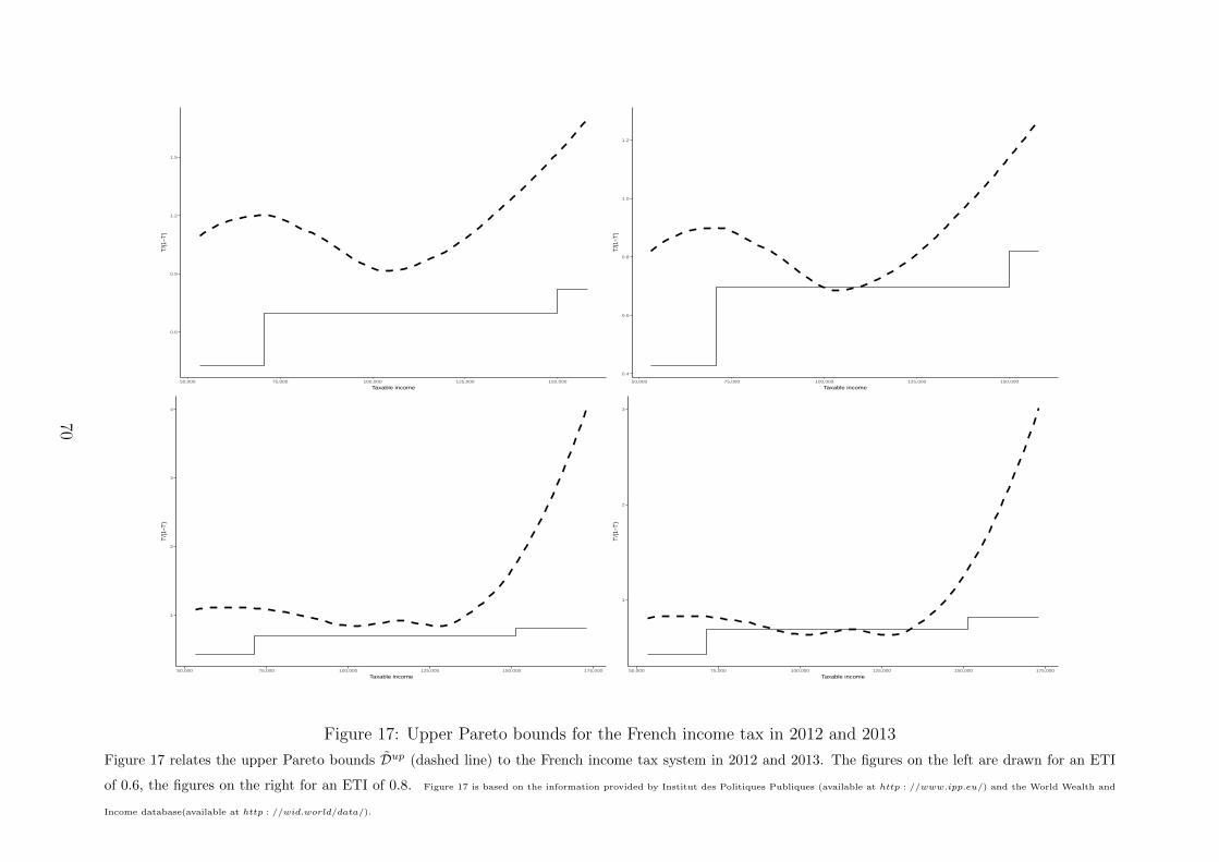
0.6

0.9

1.2

1.5

50,000 75,000 100,000 125,000 150,000

Taxable income

T'/(1

−T')

0.4

0.6

0.8

1.0

1.2

50,000 75,000 100,000 125,000 150,000

Taxable income

T'/(1

−T')

1

2

3

4

50,000 75,000 100,000 125,000 150,000 175,000

Taxable income

T'/(1

−T')

1

2

3

50,000 75,000 100,000 125,000 150,000 175,000

Taxable income

T'/(1

−T')

Figure 17: Upper Pareto bounds for the French income tax in 2012 and 2013

Figure 17 relates the upper Pareto bounds Dup (dashed line) to the French income tax system in 2012 and 2013. The figures on the left are drawn for an ETI

of 0.6, the figures on the right for an ETI of 0.8. Figure 17 is based on the information provided by Institut des Politiques Publiques (available at http : //www.ipp.eu/) and the World Wealth and

Income database(available at http : //wid.world/data/).

70

−4

−2

0

10000 20000 30000 40000

Taxable income

T'/(1

−T')

−5

−4

−3

−2

−1

0

10000 20000 30000 40000

Taxable income

T'/(1

−T')

Figure 18: Lower Pareto bounds for the UK income tax in 2012 and 2013

Figure 18 relates the lower Pareto bounds Dlow (dotted line) to the UK income tax system in 2012 (first row) and 2013 (second row) for an ETI of 0.4.

Figure 18 is based on the information provided by the United Kingdom HM Revenue & Customs (available at https : //www.gov.uk/government/collections/tax − structure − and − parameters − statistics and

https : //www.gov.uk/government/statistics/income− tax− liabilities− by − income− range−−2).

71

−10

−5

0

0 10,000 20,000 30,000 40,000 50,000

Taxable income

T'/(1

−T')

−10

−5

0

0 10000 20000 30000 40000 50000

Taxable income

T'/(1

−T')

−10

−5

0

0 10,000 20,000 30,000 40,000 50,000

Taxable income

T'/(1

−T')

−10

−5

0

0 10000 20000 30000 40000 50000

Taxable income

T'/(1

−T')

Figure 19: Lower Pareto bounds for the French income tax in 2012 and 2013

Figure 19 relates the lower Pareto bounds Dlow (dotted line) to the French income tax system in 2012 (first row) and 2013 (second row) for an ETI of 0.6. The figures

on the left are drawn for the statutory schedule taken from the OECD database and the one on the right represents the full schedule with earning subsidies for singles

without dependents taken from the TAXIPP database. Figure 19 is based on the information provided by OECD database (accessible on http : //www.oecd.org/tax/tax−policy/tax−database.htm),

the Institut des Politiques Publiques (available at http : //www.ipp.eu/), and the World Wealth and Income database (accessible on http : //wid.world/data/).

72