Political Knowledge and Misinformation in the Era of ...
29
Political Knowledge and Misinformation in the Era of Social Media: Evidence from the 2015 U.K. Election Online Appendix Kevin Munger, Patrick J. Egan , Jonathan Nagler, Jonathan Ronen, and Joshua A. Tucker March 17, 2020 APPENDIX TABLE OF CONTENTS PAGE 1: Appendix A: Details about Tweet Classification Process and Tweet Examples PAGE 4: Appendix B: Effects Plots PAGE 6: Appendix C: Full Regression Tables PAGE 11: Appendix D: Details of Survey Implementation PAGE 14: Appendix E: Effect of Topical Tweets (by Source) on Knowledge of Issue-Relevant Facts Controlling for Party ID PAGE 16: Appendix F: Weighted Regressions Using Raked Demographics from BES
Transcript of Political Knowledge and Misinformation in the Era of ...
Political Knowledge and Misinformation
in the Era of Social Media:
Evidence from the 2015 U.K. Election
Online Appendix
Kevin Munger, Patrick J. Egan
, Jonathan Nagler,
Jonathan Ronen, and Joshua A. Tucker
March 17, 2020
APPENDIX TABLE OF CONTENTS
PAGE 1: Appendix A: Details about Tweet Classification Process and Tweet
Examples
PAGE 4: Appendix B: Effects Plots
PAGE 6: Appendix C: Full Regression Tables
PAGE 11: Appendix D: Details of Survey Implementation
PAGE 14: Appendix E: Effect of Topical Tweets (by Source) on Knowledge of
Issue-Relevant Facts Controlling for Party ID
PAGE 16: Appendix F: Weighted Regressions Using Raked Demographics from
BES

PAGE 18 Appendix G: Absolute Knowledge Levels
Appendix A: Details about Tweet Classification Process andTweet Examples
As noted in the text, we selected four topics that we determined were likely tobe highly salient in the election – the economy; the U.K.’s ties to the EuropeanUnion (EU); immigration; and the fight against the ISIS terrorist organization –and identified tweets relevant to these topics. We identified all tweets on users’timelines related to these topics by first manually constructing short lists of termsrelated to each topic. We then identified which other terms most frequently co-occurred in tweets with the original anchor terms. We then used these expandedlists of terms to create our final lists of tweets related to each of the four topics.For example, we began the process of identifying tweets related to the topic of tiesto the EU by finding all tweets that included the anchor terms “Brexit” or “Euro-skeptic.” We purposefully began with this short, idiosyncratic and incompletelist in order to substantially reduce the chance of false positives. Incorporatingall tweets with these anchor terms into the subset s, we then calculated a scorereflecting the relative frequency with which any word w was found in s, weightedby how prominent w was in Twitter discussions about the topic:
Scorews =fws N
ws
fw,
where fws is the share of tweets in s including the word w, fw is the share of tweets
in our entire corpus of tweets containing word w, and Nws is the number of times
word w appeared in subset s.The following are the terms used to create each of the topics analyzed in the paper.If a tweet contained terms from multiple topics, it was labeled as belonging to eachof those topics.In implementing the keyword generation and topic-tweet matching proceduredescribed in the body of the paper, we elected to use exact token matching andavoid any pre-processing. Some of the keywords generated (eg “no2eu”) wereirregular words or contained numbers, and pre-processing steps like stemmingmight have introduced unexpected errors. The downside to this decision isprimarily in the way that variations on certain terms are included or excludedin the list of keywords: note that both “cuts” and “cut” (also “benefit” and“benefits”; “reforms” and “reform”) appear in the list of keywords for theEconomy topic, meaning that it is slightly narrower than if we had included asingle “cut[s]” token as well as the next-most-likely token. On balance, we thinkthat this decision is defensible and that the decreased risk of error outweighs thisdrawback.
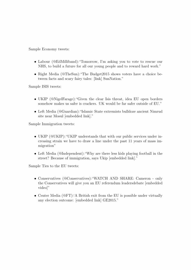
Sample Economy tweets:
• Labour (@EdMilliband):“Tomorrow, I’m asking you to vote to rescue ourNHS, to build a future for all our young people and to reward hard work.”
• Right Media (@TheSun):“The Budget2015 shows voters have a choice be-tween facts and scary fairy tales: [link] SunNation.”
Sample ISIS tweets:
• UKIP (@NigelFarage):“Given the clear Isis threat, idea EU open borderssomehow makes us safer is crackers. UK would be far safer outside of EU.”
• Left Media (@Guardian):“Islamic State extremists bulldoze ancient Nimrudsite near Mosul [embedded link].”
Sample Immigration tweets:
• UKIP (@UKIP):“UKIP understands that with our public services under in-creasing strain we have to draw a line under the past 11 years of mass im-migration”
• Left Media (@Independent):“Why are there less kids playing football in thestreet? Because of immigration, says Ukip [embedded link].”
Sample Ties to the EU tweets:
• Conservatives (@Conservatives):“WATCH AND SHARE: Cameron - onlythe Conservatives will give you an EU referendum leadersdebate [embeddedvideo]”
• Center Media (@FT):‘A British exit from the EU is possible under virtuallyany election outcome: [embedded link] GE2015.”
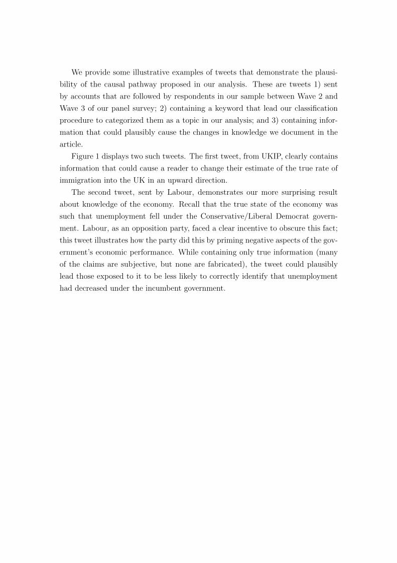
We provide some illustrative examples of tweets that demonstrate the plausi-
bility of the causal pathway proposed in our analysis. These are tweets 1) sent
by accounts that are followed by respondents in our sample between Wave 2 and
Wave 3 of our panel survey; 2) containing a keyword that lead our classification
procedure to categorized them as a topic in our analysis; and 3) containing infor-
mation that could plausibly cause the changes in knowledge we document in the
article.
Figure 1 displays two such tweets. The first tweet, from UKIP, clearly contains
information that could cause a reader to change their estimate of the true rate of
immigration into the UK in an upward direction.
The second tweet, sent by Labour, demonstrates our more surprising result
about knowledge of the economy. Recall that the true state of the economy was
such that unemployment fell under the Conservative/Liberal Democrat govern-
ment. Labour, as an opposition party, faced a clear incentive to obscure this fact;
this tweet illustrates how the party did this by priming negative aspects of the gov-
ernment’s economic performance. While containing only true information (many
of the claims are subjective, but none are fabricated), the tweet could plausibly
lead those exposed to it to be less likely to correctly identify that unemployment
had decreased under the incumbent government.
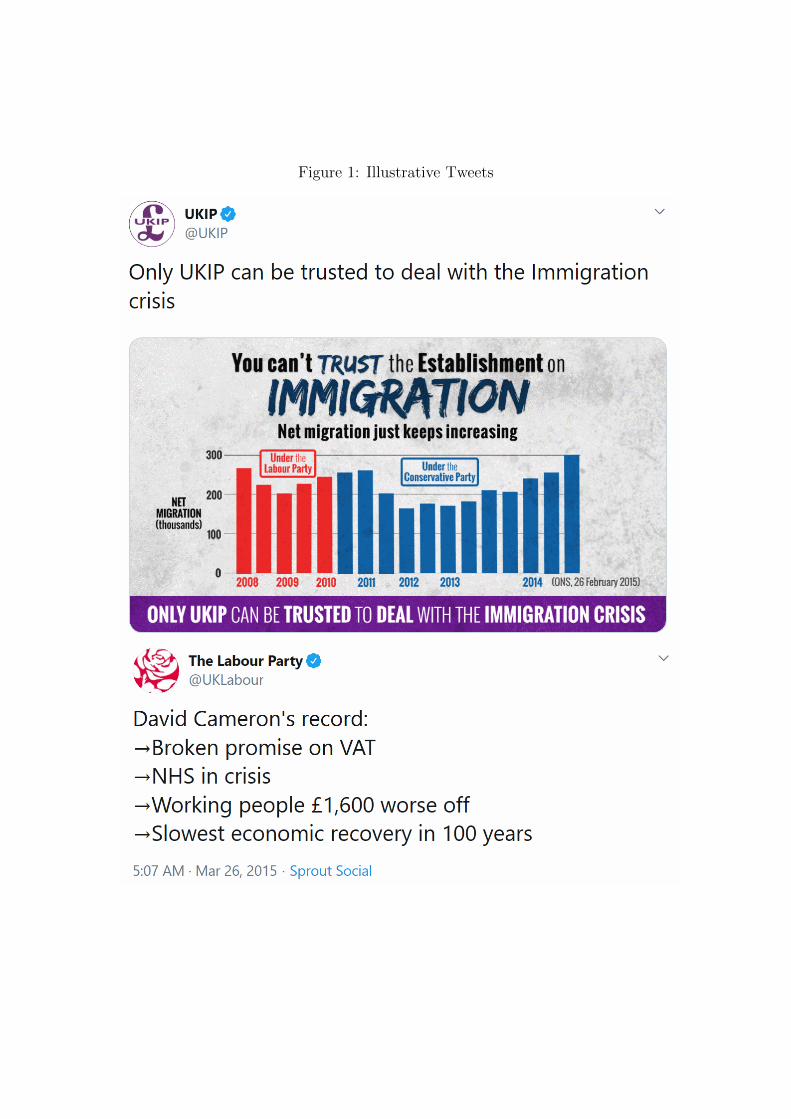
Figure 1: Illustrative Tweets
Appendix B: Effects Plots
Immigration: Effect of Media
Log of Relevant Political Tweets
Pro
babl
ity o
f Cor
rect
Ran
king
W4
0.70
0.75
0.80
0.85
0 2 4 6 8 10
Immigration: Effect of Political Parties
Log of Relevant Political TweetsP
roba
blity
of C
orre
ct R
anki
ng W
4
0.72
0.74
0.76
0.78
0.80
0.82
0.84
0.86
0 2 4 6 8 10
Spending: Effect of Media
Log of Relevant Political Tweets
Pro
babl
ity o
f Cor
rect
Ran
king
W4
0.40
0.45
0.50
0.55
0.60
0.65
0 2 4 6 8 10
Spending: Effect of Political Parties
Log of Relevant Political Tweets
Pro
babl
ity o
f Cor
rect
Ran
king
W4
0.55
0.60
0.65
0.70
0.75
0.80
0 2 4 6 8 10
EU: Effect of Media
Log of Relevant Political Tweets
Pro
babl
ity o
f Cor
rect
Ran
king
W4
0.80
0.85
0.90
0 2 4 6 8 10
EU: Effect of Political Parties
Log of Relevant Political Tweets
Pro
babl
ity o
f Cor
rect
Ran
king
W4
0.82
0.84
0.86
0.88
0.90
0.92
0.94
0 2 4 6 8 10
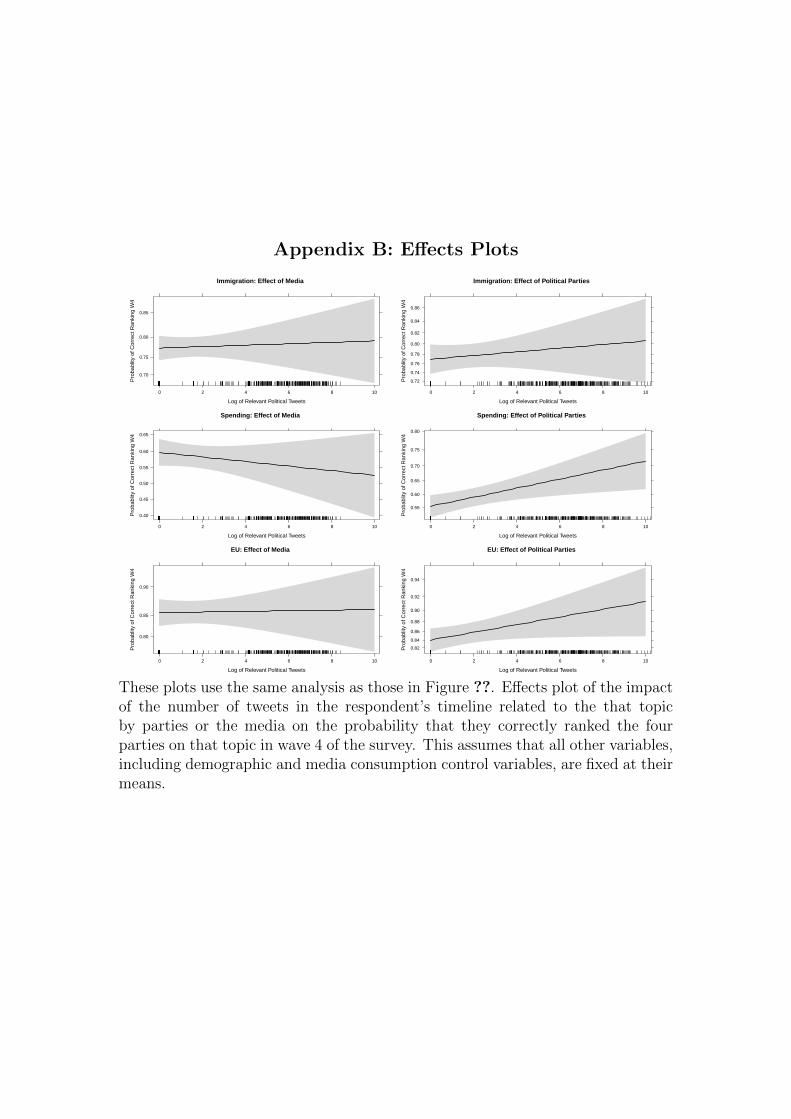
These plots use the same analysis as those in Figure ??. Effects plot of the impactof the number of tweets in the respondent’s timeline related to the that topicby parties or the media on the probability that they correctly ranked the fourparties on that topic in wave 4 of the survey. This assumes that all other variables,including demographic and media consumption control variables, are fixed at theirmeans.
Log of Relevant Political Tweets
Pro
babl
ity o
f Cor
rect
Ans
wer
W3
0.45
0.50
0.55
0.60
0.65
0.70
0 2 4 6 8 10
Log of Relevant Political Tweets
Pro
babl
ity o
f Cor
rect
Ans
wer
W3
0.80
0.85
0.90
0.95
0 2 4 6 8 10
Log of Relevant Political Tweets
Pro
babl
ity o
f Cor
rect
Ans
wer
W3
0.50
0.55
0.60
0.65
0 2 4 6 8 10
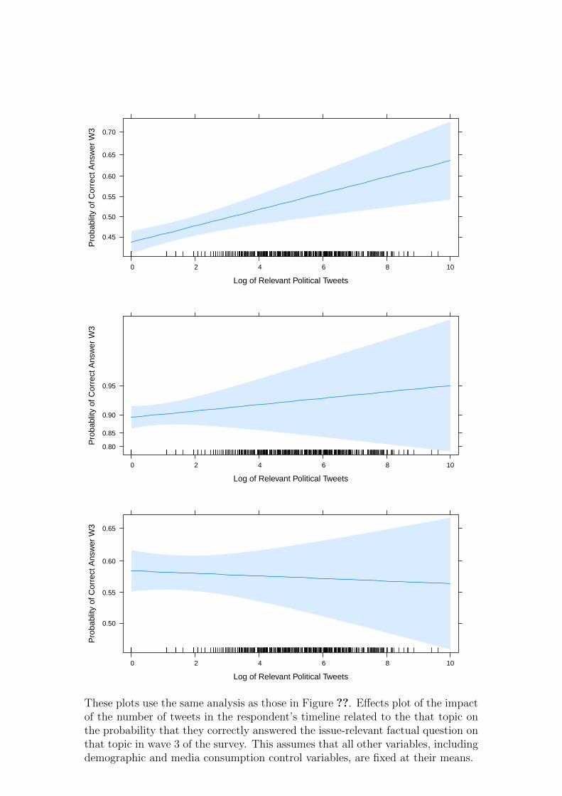
These plots use the same analysis as those in Figure ??. Effects plot of the impactof the number of tweets in the respondent’s timeline related to the that topic onthe probability that they correctly answered the issue-relevant factual question onthat topic in wave 3 of the survey. This assumes that all other variables, includingdemographic and media consumption control variables, are fixed at their means.
Immigration: Effect of Media
Log of Relevant Political Tweets
Pro
babl
ity o
f Cor
rect
Ans
wer
W3
0.45
0.50
0.55
0.60
0.65
0.70
0.75
0.80
0 2 4 6 8 10
Immigration: Effect of Political Parties
Log of Relevant Political Tweets
Pro
babl
ity o
f Cor
rect
Ans
wer
W3
0.40
0.45
0.50
0.55
0.60
0.65
0 2 4 6 8 10
Unemployment: Effect of Media
Log of Relevant Political Tweets
Pro
babl
ity o
f Cor
rect
Ans
wer
W3
0.55
0.60
0.65
0.70
0.75
0.80
0.85
0 2 4 6 8 10
Unemployment: Effect of Political Parties
Log of Relevant Political Tweets
Pro
babl
ity o
f Cor
rect
Ans
wer
W3
0.30
0.35
0.40
0.45
0.50
0.55
0.60
0 2 4 6 8 10
ISIS: Effect of Media
Log of Relevant Political Tweets
Pro
babl
ity o
f Cor
rect
Ans
wer
W3
0.850.90
0.95
0 2 4 6 8 10
ISIS: Effect of Political Parties
Log of Relevant Political Tweets
Pro
babl
ity o
f Cor
rect
Ans
wer
W3
0.3
0.4
0.5
0.6
0.7
0.8
0.9
0 2 4 6 8 10
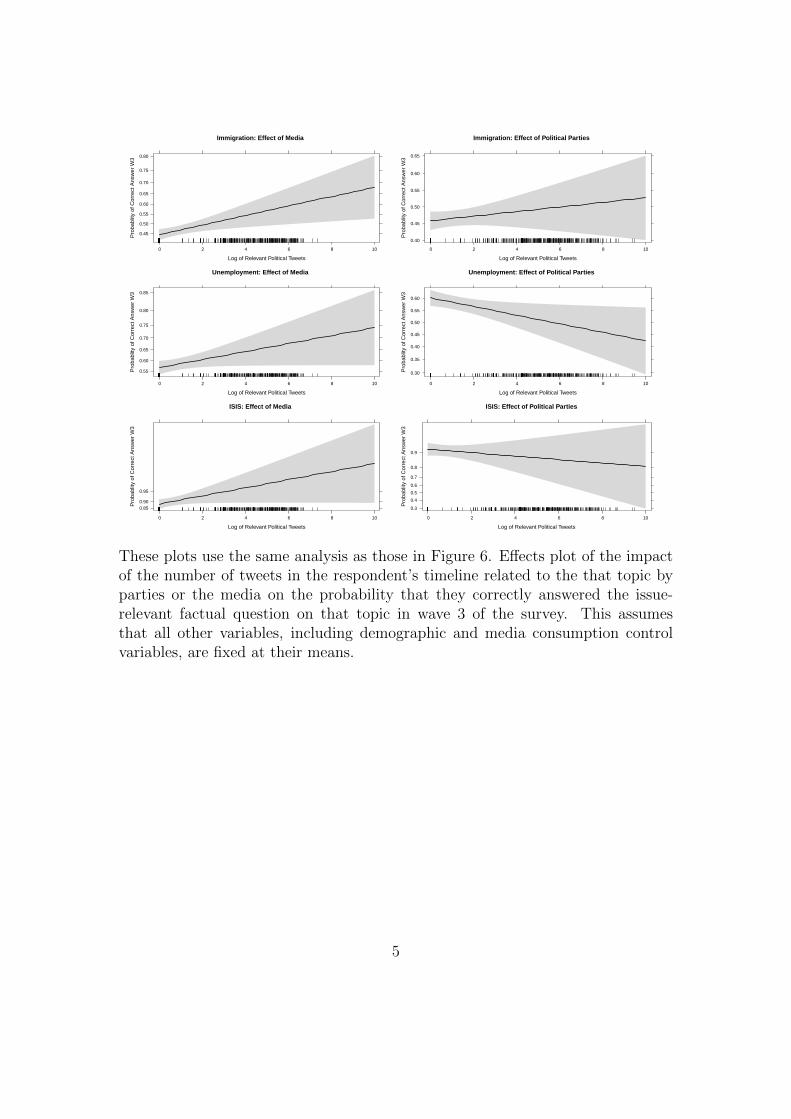
These plots use the same analysis as those in Figure 6. Effects plot of the impactof the number of tweets in the respondent’s timeline related to the that topic byparties or the media on the probability that they correctly answered the issue-relevant factual question on that topic in wave 3 of the survey. This assumesthat all other variables, including demographic and media consumption controlvariables, are fixed at their means.
5
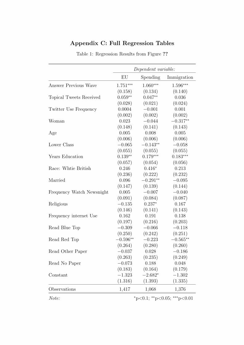
Appendix C: Full Regression Tables
Table 1: Regression Results from Figure ??
Dependent variable:
EU Spending Immigration
Answer Previous Wave 1.751∗∗∗ 1.060∗∗∗ 1.596∗∗∗
(0.158) (0.134) (0.140)Topical Tweets Received 0.059∗∗ 0.047∗∗ 0.036
(0.028) (0.021) (0.024)Twitter Use Frequency 0.0004 −0.001 0.001
(0.002) (0.002) (0.002)Woman 0.023 −0.044 −0.317∗∗
(0.148) (0.141) (0.143)Age 0.005 0.008 0.005
(0.006) (0.006) (0.006)Lower Class −0.065 −0.143∗∗ −0.058
(0.055) (0.055) (0.055)Years Education 0.139∗∗ 0.179∗∗∗ 0.183∗∗∗
(0.057) (0.054) (0.056)Race: Whtie British 0.246 0.416∗ 0.213
(0.236) (0.222) (0.232)Married 0.096 −0.291∗∗ −0.095
(0.147) (0.139) (0.144)Frequency Watch Newsnight 0.005 −0.007 −0.040
(0.091) (0.084) (0.087)Religious −0.135 0.237∗ 0.167
(0.146) (0.141) (0.143)Frequency internet Use 0.162 0.191 0.138
(0.197) (0.216) (0.203)Read Blue Top −0.309 −0.066 −0.118
(0.250) (0.242) (0.251)Read Red Top −0.596∗∗ −0.223 −0.565∗∗
(0.264) (0.280) (0.260)Read Other Paper −0.037 0.028 −0.186
(0.263) (0.235) (0.249)Read No Paper −0.073 0.188 0.048
(0.183) (0.164) (0.179)Constant −1.323 −2.682∗ −1.302
(1.316) (1.393) (1.335)
Observations 1,417 1,068 1,376
Note: ∗p<0.1; ∗∗p<0.05; ∗∗∗p<0.01
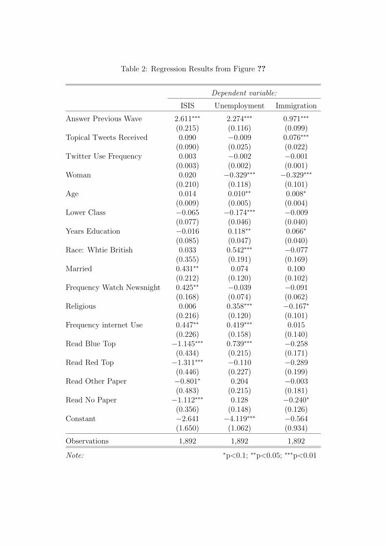
Table 2: Regression Results from Figure ??
Dependent variable:
ISIS Unemployment Immigration
Answer Previous Wave 2.611∗∗∗ 2.274∗∗∗ 0.971∗∗∗
(0.215) (0.116) (0.099)Topical Tweets Received 0.090 −0.009 0.076∗∗∗
(0.090) (0.025) (0.022)Twitter Use Frequency 0.003 −0.002 −0.001
(0.003) (0.002) (0.001)Woman 0.020 −0.329∗∗∗ −0.329∗∗∗
(0.210) (0.118) (0.101)Age 0.014 0.010∗∗ 0.008∗
(0.009) (0.005) (0.004)Lower Class −0.065 −0.174∗∗∗ −0.009
(0.077) (0.046) (0.040)Years Education −0.016 0.118∗∗ 0.066∗
(0.085) (0.047) (0.040)Race: Whtie British 0.033 0.542∗∗∗ −0.077
(0.355) (0.191) (0.169)Married 0.431∗∗ 0.074 0.100
(0.212) (0.120) (0.102)Frequency Watch Newsnight 0.425∗∗ −0.039 −0.091
(0.168) (0.074) (0.062)Religious 0.006 0.358∗∗∗ −0.167∗
(0.216) (0.120) (0.101)Frequency internet Use 0.447∗∗ 0.419∗∗∗ 0.015
(0.226) (0.158) (0.140)Read Blue Top −1.145∗∗∗ 0.739∗∗∗ −0.258
(0.434) (0.215) (0.171)Read Red Top −1.311∗∗∗ −0.110 −0.289
(0.446) (0.227) (0.199)Read Other Paper −0.801∗ 0.204 −0.003
(0.483) (0.215) (0.181)Read No Paper −1.112∗∗∗ 0.128 −0.240∗
(0.356) (0.148) (0.126)Constant −2.641 −4.119∗∗∗ −0.564
(1.650) (1.062) (0.934)
Observations 1,892 1,892 1,892
Note: ∗p<0.1; ∗∗p<0.05; ∗∗∗p<0.01
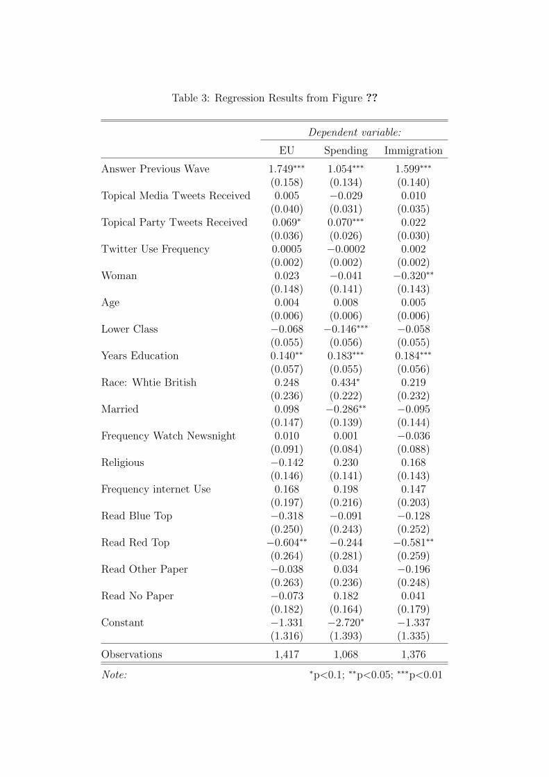
Table 3: Regression Results from Figure ??
Dependent variable:
EU Spending Immigration
Answer Previous Wave 1.749∗∗∗ 1.054∗∗∗ 1.599∗∗∗
(0.158) (0.134) (0.140)Topical Media Tweets Received 0.005 −0.029 0.010
(0.040) (0.031) (0.035)Topical Party Tweets Received 0.069∗ 0.070∗∗∗ 0.022
(0.036) (0.026) (0.030)Twitter Use Frequency 0.0005 −0.0002 0.002
(0.002) (0.002) (0.002)Woman 0.023 −0.041 −0.320∗∗
(0.148) (0.141) (0.143)Age 0.004 0.008 0.005
(0.006) (0.006) (0.006)Lower Class −0.068 −0.146∗∗∗ −0.058
(0.055) (0.056) (0.055)Years Education 0.140∗∗ 0.183∗∗∗ 0.184∗∗∗
(0.057) (0.055) (0.056)Race: Whtie British 0.248 0.434∗ 0.219
(0.236) (0.222) (0.232)Married 0.098 −0.286∗∗ −0.095
(0.147) (0.139) (0.144)Frequency Watch Newsnight 0.010 0.001 −0.036
(0.091) (0.084) (0.088)Religious −0.142 0.230 0.168
(0.146) (0.141) (0.143)Frequency internet Use 0.168 0.198 0.147
(0.197) (0.216) (0.203)Read Blue Top −0.318 −0.091 −0.128
(0.250) (0.243) (0.252)Read Red Top −0.604∗∗ −0.244 −0.581∗∗
(0.264) (0.281) (0.259)Read Other Paper −0.038 0.034 −0.196
(0.263) (0.236) (0.248)Read No Paper −0.073 0.182 0.041
(0.182) (0.164) (0.179)Constant −1.331 −2.720∗ −1.337
(1.316) (1.393) (1.335)
Observations 1,417 1,068 1,376
Note: ∗p<0.1; ∗∗p<0.05; ∗∗∗p<0.01
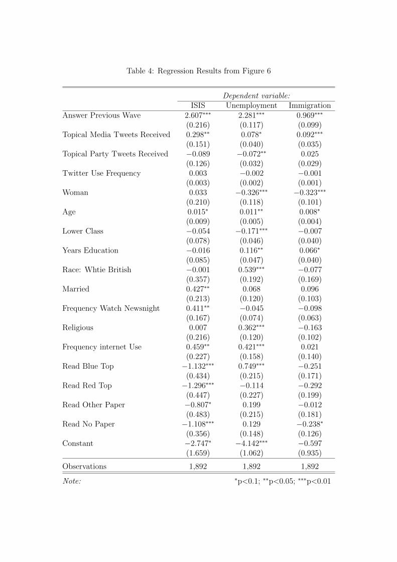
Table 4: Regression Results from Figure 6
Dependent variable:ISIS Unemployment Immigration
Answer Previous Wave 2.607∗∗∗ 2.281∗∗∗ 0.969∗∗∗
(0.216) (0.117) (0.099)Topical Media Tweets Received 0.298∗∗ 0.078∗ 0.092∗∗∗
(0.151) (0.040) (0.035)Topical Party Tweets Received −0.089 −0.072∗∗ 0.025
(0.126) (0.032) (0.029)Twitter Use Frequency 0.003 −0.002 −0.001
(0.003) (0.002) (0.001)Woman 0.033 −0.326∗∗∗ −0.323∗∗∗
(0.210) (0.118) (0.101)Age 0.015∗ 0.011∗∗ 0.008∗
(0.009) (0.005) (0.004)Lower Class −0.054 −0.171∗∗∗ −0.007
(0.078) (0.046) (0.040)Years Education −0.016 0.116∗∗ 0.066∗
(0.085) (0.047) (0.040)Race: Whtie British −0.001 0.539∗∗∗ −0.077
(0.357) (0.192) (0.169)Married 0.427∗∗ 0.068 0.096
(0.213) (0.120) (0.103)Frequency Watch Newsnight 0.411∗∗ −0.045 −0.098
(0.167) (0.074) (0.063)Religious 0.007 0.362∗∗∗ −0.163
(0.216) (0.120) (0.102)Frequency internet Use 0.459∗∗ 0.421∗∗∗ 0.021
(0.227) (0.158) (0.140)Read Blue Top −1.132∗∗∗ 0.749∗∗∗ −0.251
(0.434) (0.215) (0.171)Read Red Top −1.296∗∗∗ −0.114 −0.292
(0.447) (0.227) (0.199)Read Other Paper −0.807∗ 0.199 −0.012
(0.483) (0.215) (0.181)Read No Paper −1.108∗∗∗ 0.129 −0.238∗
(0.356) (0.148) (0.126)Constant −2.747∗ −4.142∗∗∗ −0.597
(1.659) (1.062) (0.935)
Observations 1,892 1,892 1,892
Note: ∗p<0.1; ∗∗p<0.05; ∗∗∗p<0.01
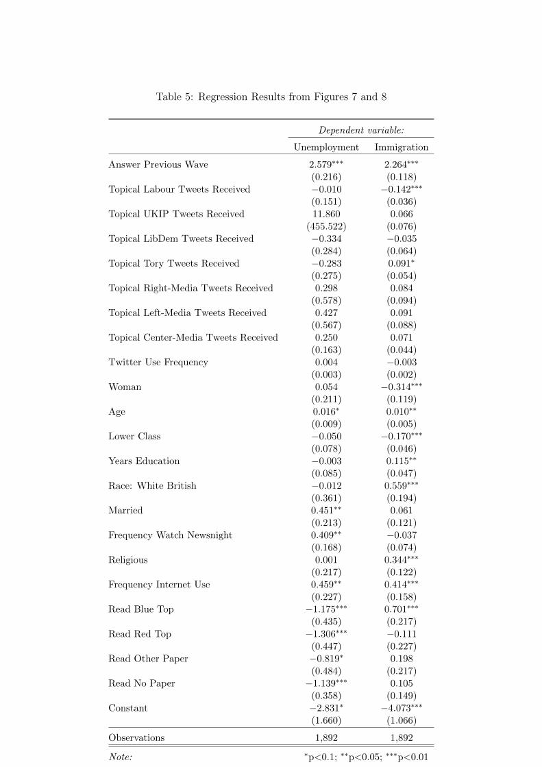
Table 5: Regression Results from Figures 7 and 8
Dependent variable:
Unemployment Immigration
Answer Previous Wave 2.579∗∗∗ 2.264∗∗∗
(0.216) (0.118)Topical Labour Tweets Received −0.010 −0.142∗∗∗
(0.151) (0.036)Topical UKIP Tweets Received 11.860 0.066
(455.522) (0.076)Topical LibDem Tweets Received −0.334 −0.035
(0.284) (0.064)Topical Tory Tweets Received −0.283 0.091∗
(0.275) (0.054)Topical Right-Media Tweets Received 0.298 0.084
(0.578) (0.094)Topical Left-Media Tweets Received 0.427 0.091
(0.567) (0.088)Topical Center-Media Tweets Received 0.250 0.071
(0.163) (0.044)Twitter Use Frequency 0.004 −0.003
(0.003) (0.002)Woman 0.054 −0.314∗∗∗
(0.211) (0.119)Age 0.016∗ 0.010∗∗
(0.009) (0.005)Lower Class −0.050 −0.170∗∗∗
(0.078) (0.046)Years Education −0.003 0.115∗∗
(0.085) (0.047)Race: White British −0.012 0.559∗∗∗
(0.361) (0.194)Married 0.451∗∗ 0.061
(0.213) (0.121)Frequency Watch Newsnight 0.409∗∗ −0.037
(0.168) (0.074)Religious 0.001 0.344∗∗∗
(0.217) (0.122)Frequency Internet Use 0.459∗∗ 0.414∗∗∗
(0.227) (0.158)Read Blue Top −1.175∗∗∗ 0.701∗∗∗
(0.435) (0.217)Read Red Top −1.306∗∗∗ −0.111
(0.447) (0.227)Read Other Paper −0.819∗ 0.198
(0.484) (0.217)Read No Paper −1.139∗∗∗ 0.105
(0.358) (0.149)Constant −2.831∗ −4.073∗∗∗
(1.660) (1.066)
Observations 1,892 1,892
Note: ∗p<0.1; ∗∗p<0.05; ∗∗∗p<0.01
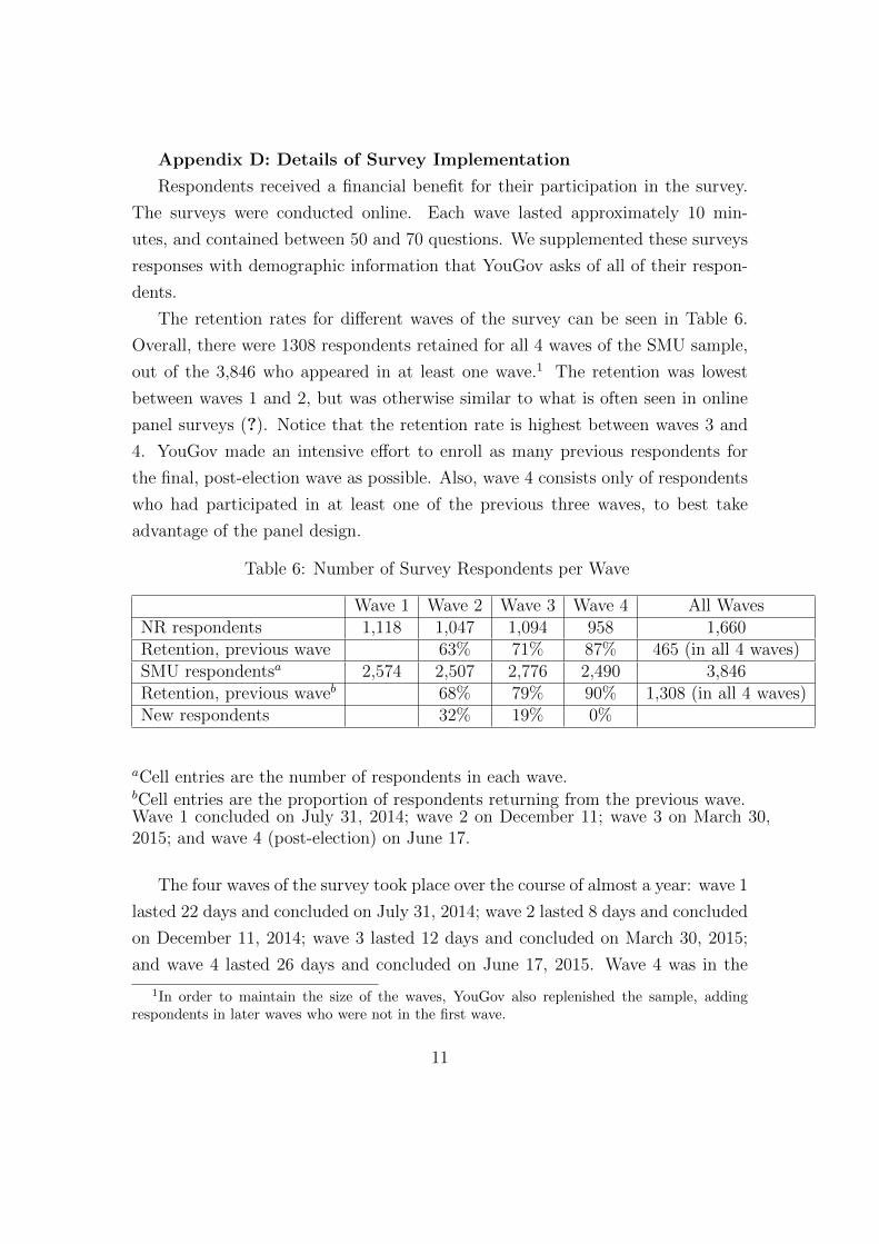
Appendix D: Details of Survey Implementation
Respondents received a financial benefit for their participation in the survey.
The surveys were conducted online. Each wave lasted approximately 10 min-
utes, and contained between 50 and 70 questions. We supplemented these surveys
responses with demographic information that YouGov asks of all of their respon-
dents.
The retention rates for different waves of the survey can be seen in Table 6.
Overall, there were 1308 respondents retained for all 4 waves of the SMU sample,
out of the 3,846 who appeared in at least one wave.1 The retention was lowest
between waves 1 and 2, but was otherwise similar to what is often seen in online
panel surveys (?). Notice that the retention rate is highest between waves 3 and
4. YouGov made an intensive effort to enroll as many previous respondents for
the final, post-election wave as possible. Also, wave 4 consists only of respondents
who had participated in at least one of the previous three waves, to best take
advantage of the panel design.
Table 6: Number of Survey Respondents per Wave
Wave 1 Wave 2 Wave 3 Wave 4 All WavesNR respondents 1,118 1,047 1,094 958 1,660Retention, previous wave 63% 71% 87% 465 (in all 4 waves)SMU respondentsa 2,574 2,507 2,776 2,490 3,846Retention, previous waveb 68% 79% 90% 1,308 (in all 4 waves)New respondents 32% 19% 0%
aCell entries are the number of respondents in each wave.bCell entries are the proportion of respondents returning from the previous wave.Wave 1 concluded on July 31, 2014; wave 2 on December 11; wave 3 on March 30,2015; and wave 4 (post-election) on June 17.
The four waves of the survey took place over the course of almost a year: wave 1
lasted 22 days and concluded on July 31, 2014; wave 2 lasted 8 days and concluded
on December 11, 2014; wave 3 lasted 12 days and concluded on March 30, 2015;
and wave 4 lasted 26 days and concluded on June 17, 2015. Wave 4 was in the
1In order to maintain the size of the waves, YouGov also replenished the sample, addingrespondents in later waves who were not in the first wave.
11
field for an especially long time as part of the effort to increase the retention rate,
and it began 2 weeks after the day of the general election on May 7, 2015.
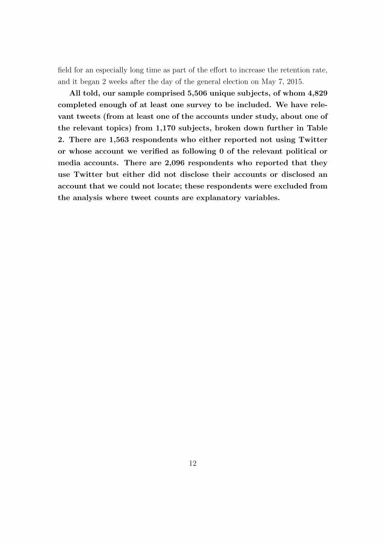
All told, our sample comprised 5,506 unique subjects, of whom 4,829
completed enough of at least one survey to be included. We have rele-
vant tweets (from at least one of the accounts under study, about one of
the relevant topics) from 1,170 subjects, broken down further in Table
2. There are 1,563 respondents who either reported not using Twitter
or whose account we verified as following 0 of the relevant political or
media accounts. There are 2,096 respondents who reported that they
use Twitter but either did not disclose their accounts or disclosed an
account that we could not locate; these respondents were excluded from
the analysis where tweet counts are explanatory variables.
12
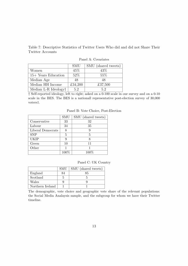
Table 7: Descriptive Statistics of Twitter Users Who did and did not Share TheirTwitter Accounts
Panel A: Covariates
SMU SMU (shared tweets)Women 45% 43%15+ Years Education 52% 55%Median Age 48 48Median HH Income £34,200 £37,500Median L-R Ideology† 5.2 5.2† Self-reported ideology, left to right; asked on a 0-100 scale in our survey and on a 0-10scale in the BES. The BES is a nationall representative post-election survey of 30,000voters1.
Panel B: Vote Choice, Post-Election
SMU SMU (shared tweets)
Conservative 33 32
Labour 34 35
Liberal Democrats 8 9
SNP 5 5
UKIP 9 8
Green 10 11
Other 1 1
100% 100%
Panel C: UK Country
SMU SMU (shared tweets)
England 84 85
Scotland 5 5
Wales 9 9
Northern Ireland 1 1
The demographic, vote choice and geographic vote share of the relevant populations:the Social Media Analaysis sample, and the subgroup for whom we have their Twittertimeline.
13
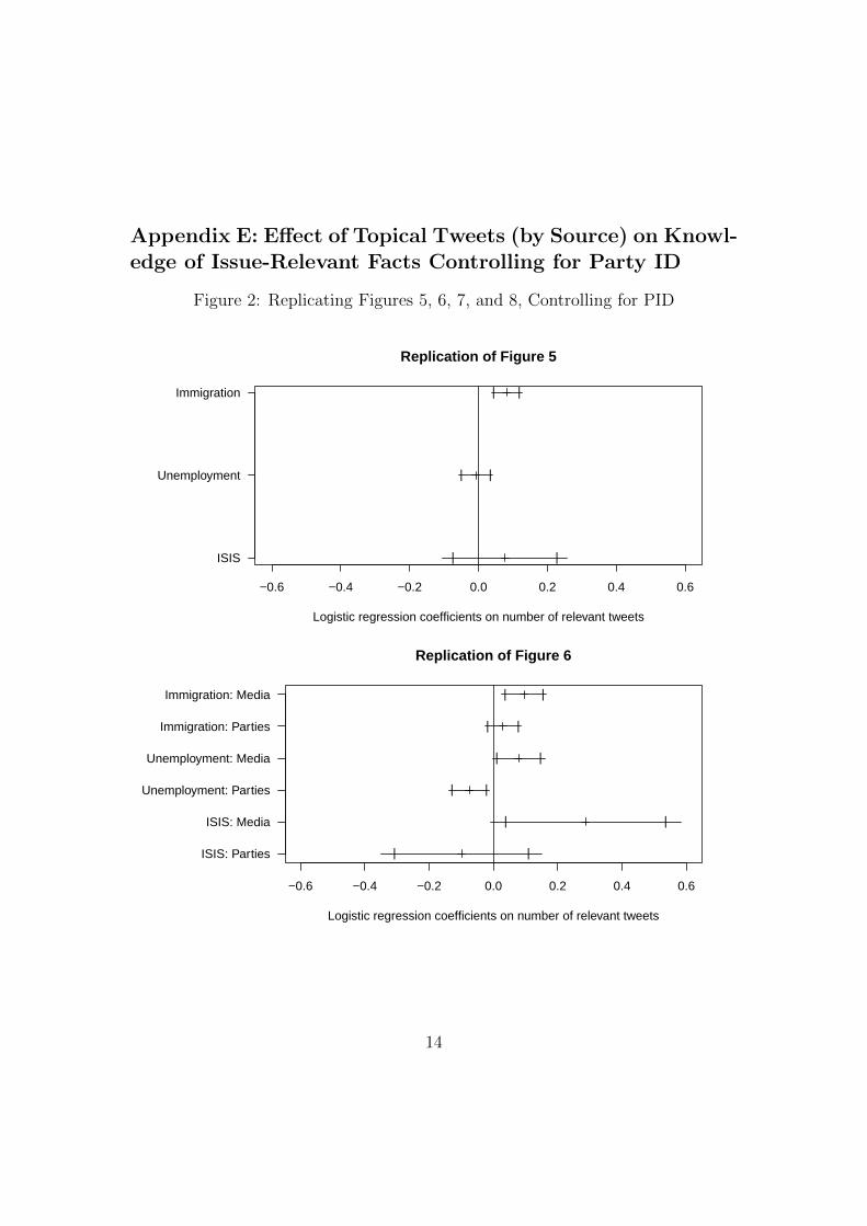
Appendix E: Effect of Topical Tweets (by Source) on Knowl-edge of Issue-Relevant Facts Controlling for Party ID
Figure 2: Replicating Figures 5, 6, 7, and 8, Controlling for PID
−0.6 −0.4 −0.2 0.0 0.2 0.4 0.6
Replication of Figure 5
Logistic regression coefficients on number of relevant tweets
ISIS
Unemployment
Immigration
|
|
|
|
|
|
−0.6 −0.4 −0.2 0.0 0.2 0.4 0.6
Replication of Figure 6
Logistic regression coefficients on number of relevant tweets
ISIS: Parties
ISIS: Media
Unemployment: Parties
Unemployment: Media
Immigration: Parties
Immigration: Media
|
|
|
|
|
|
|
|
|
|
|
|
14
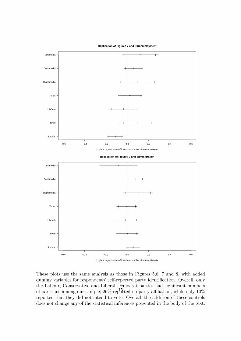
−0.6 −0.4 −0.2 0.0 0.2 0.4 0.6
Replication of Figures 7 and 8:Unemployment
Logistic regression coefficients on number of relevant tweets
Labour
UKIP
LibDem
Tories
Right media
Cent media
Left media
|
|
|
|
|
|
|
|
|
|
|
|
|
|
−0.6 −0.4 −0.2 0.0 0.2 0.4 0.6
Replication of Figures 7 and 8:Immigration
Logistic regression coefficients on number of relevant tweets
Labour
UKIP
LibDem
Tories
Right media
Cent media
Left media
|
|
|
|
|
|
|
|
|
|
|
|
|
|
These plots use the same analysis as those in Figures 5,6, 7 and 8, with addeddummy variables for respondents’ self-reported party identification. Overall, onlythe Labour, Conservative and Liberal Democrat parties had significant numbersof partisans among our sample; 26% reported no party affiliation, while only 10%reported that they did not intend to vote. Overall, the addition of these controlsdoes not change any of the statistical inferences presented in the body of the text.
15
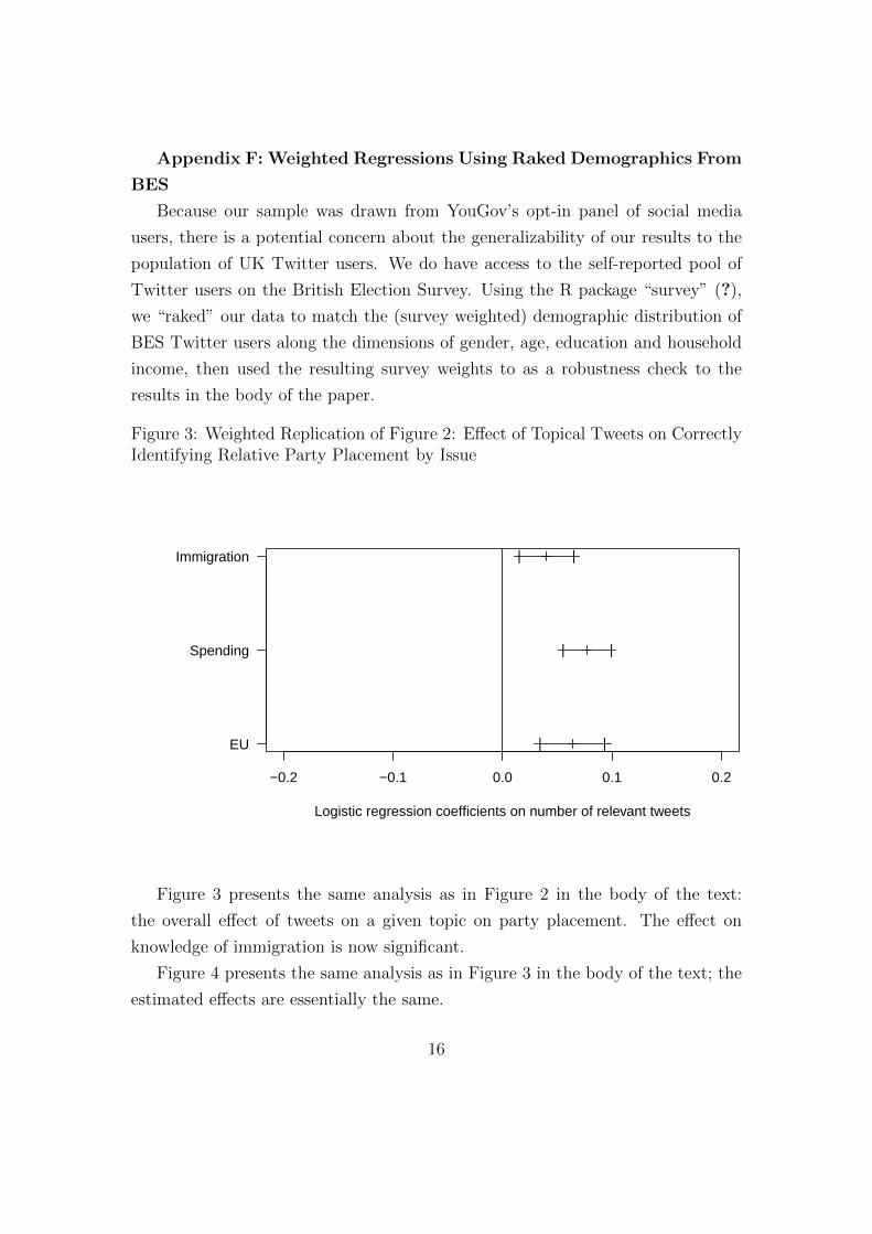
Appendix F: Weighted Regressions Using Raked Demographics From
BES
Because our sample was drawn from YouGov’s opt-in panel of social media
users, there is a potential concern about the generalizability of our results to the
population of UK Twitter users. We do have access to the self-reported pool of
Twitter users on the British Election Survey. Using the R package “survey” (?),
we “raked” our data to match the (survey weighted) demographic distribution of
BES Twitter users along the dimensions of gender, age, education and household
income, then used the resulting survey weights to as a robustness check to the
results in the body of the paper.
Figure 3: Weighted Replication of Figure 2: Effect of Topical Tweets on CorrectlyIdentifying Relative Party Placement by Issue
−0.2 −0.1 0.0 0.1 0.2
Logistic regression coefficients on number of relevant tweets
EU
Spending
Immigration
|
|
|
|
|
|
Figure 3 presents the same analysis as in Figure 2 in the body of the text:
the overall effect of tweets on a given topic on party placement. The effect on
knowledge of immigration is now significant.
Figure 4 presents the same analysis as in Figure 3 in the body of the text; the
estimated effects are essentially the same.
16
Figure 5 presents the same analysis as in Figure 4 in the body of the text:
the overall effect of tweets on a given topic on party placement, disaggregated by
source. The effect of media tweets on party placement on the topic of immigration
is now significant; the rest of the results are largely unchanged.
Figure 7 presents the same analysis as in Figure 6 in the body of the text:
the overall effect of tweets on a given topic on factual knowledge, divided by the
source of the tweeter (media or politicians). The effects are essentially the same,
although better estimated.
Figure 8 presents the same analysis as in Figure 7 in the body of the text:
the effect of tweets on factual knowledge of unemployment, divided by the source
of the tweeter. Here, the results provide considerably stronger evidence for our
theory than the results from the unweighted regression in the body of the paper.
Each of the media-ideology clusters effects’ is now estimated as positive and
significant. But more notably, the effect of tweets from Liberal Democrats goes
from slightly negative to positive and significant. The latter better fits our theory,
as the Liberal Democrats were involved with the coalition government during the
election and thus had the same incentive to promulgate knowledge of the low
unemployment rate at the time. Furthermore, this result is not cherry-picked: this
is the only instance where the addition of the survey weights raked from the BES
causes a coefficient estimate to switch signs and become statistically significant.
The estimated effect of tweets from the challenger Labour party remains a
statistically significant reduction in knowledge of the positive economic situation.
Figure 9 presents the same analysis as in Figure 8 in the body of the text: the
effect of tweets on factual knowledge of immigration, divided by the source of the
tweeter. The effects are essentially the same, although better estimated.
17
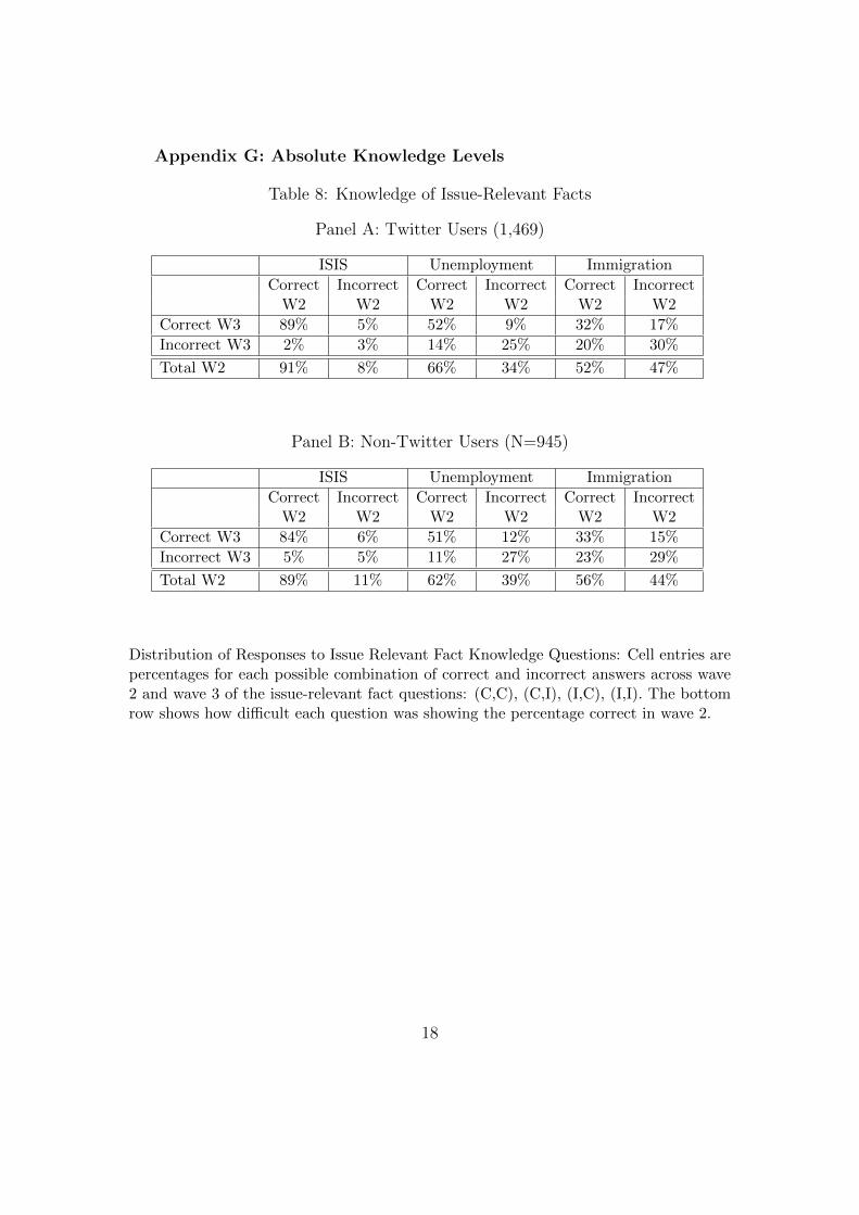
Appendix G: Absolute Knowledge Levels
Table 8: Knowledge of Issue-Relevant Facts
Panel A: Twitter Users (1,469)
ISIS Unemployment Immigration
Correct Incorrect Correct Incorrect Correct IncorrectW2 W2 W2 W2 W2 W2
Correct W3 89% 5% 52% 9% 32% 17%
Incorrect W3 2% 3% 14% 25% 20% 30%
Total W2 91% 8% 66% 34% 52% 47%
Panel B: Non-Twitter Users (N=945)
ISIS Unemployment Immigration
Correct Incorrect Correct Incorrect Correct IncorrectW2 W2 W2 W2 W2 W2
Correct W3 84% 6% 51% 12% 33% 15%
Incorrect W3 5% 5% 11% 27% 23% 29%
Total W2 89% 11% 62% 39% 56% 44%
Distribution of Responses to Issue Relevant Fact Knowledge Questions: Cell entries arepercentages for each possible combination of correct and incorrect answers across wave2 and wave 3 of the issue-relevant fact questions: (C,C), (C,I), (I,C), (I,I). The bottomrow shows how difficult each question was showing the percentage correct in wave 2.
18
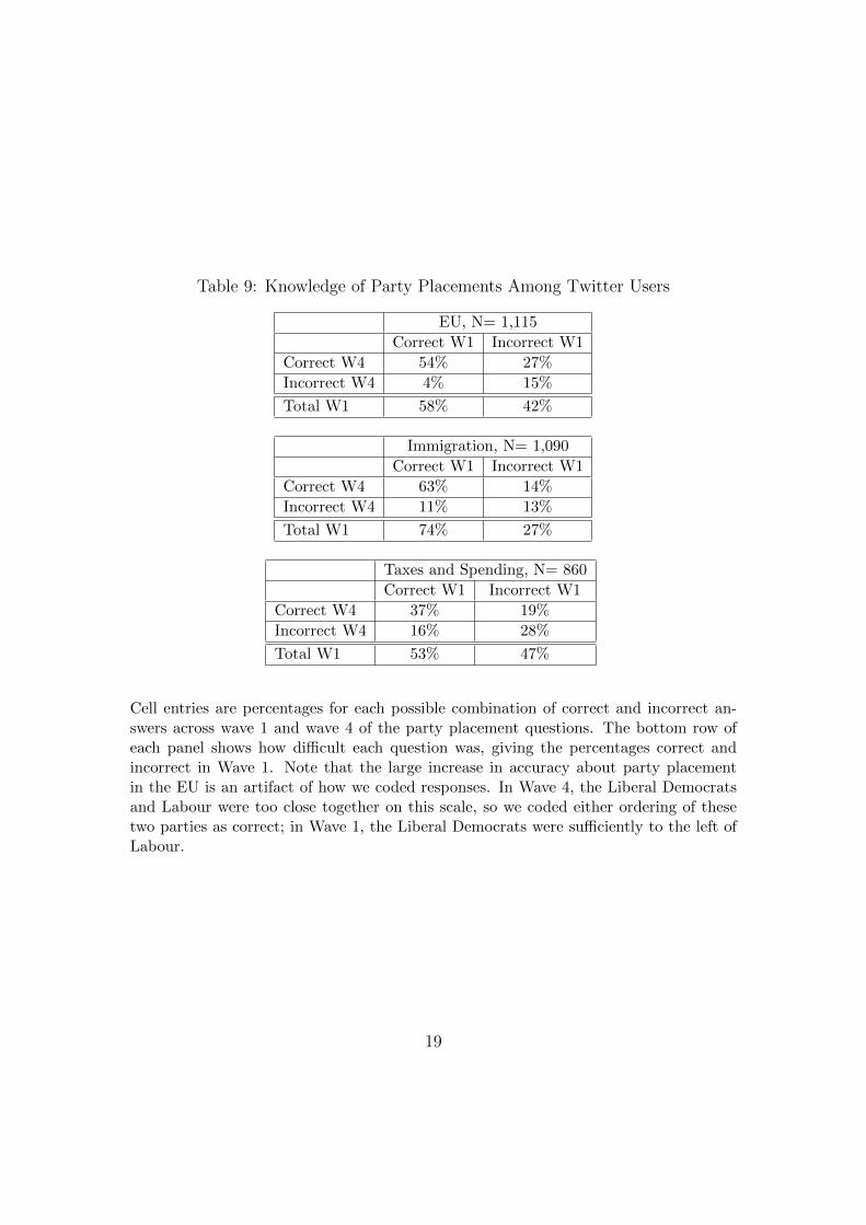
Table 9: Knowledge of Party Placements Among Twitter Users
EU, N= 1,115
Correct W1 Incorrect W1
Correct W4 54% 27%
Incorrect W4 4% 15%
Total W1 58% 42%
Immigration, N= 1,090
Correct W1 Incorrect W1
Correct W4 63% 14%
Incorrect W4 11% 13%
Total W1 74% 27%
Taxes and Spending, N= 860
Correct W1 Incorrect W1
Correct W4 37% 19%
Incorrect W4 16% 28%
Total W1 53% 47%
Cell entries are percentages for each possible combination of correct and incorrect an-swers across wave 1 and wave 4 of the party placement questions. The bottom row ofeach panel shows how difficult each question was, giving the percentages correct andincorrect in Wave 1. Note that the large increase in accuracy about party placementin the EU is an artifact of how we coded responses. In Wave 4, the Liberal Democratsand Labour were too close together on this scale, so we coded either ordering of thesetwo parties as correct; in Wave 1, the Liberal Democrats were sufficiently to the left ofLabour.
19
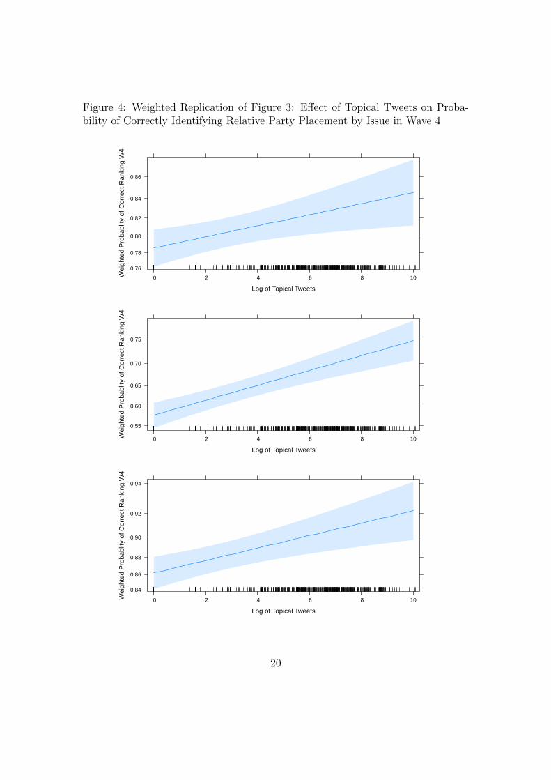
Figure 4: Weighted Replication of Figure 3: Effect of Topical Tweets on Proba-bility of Correctly Identifying Relative Party Placement by Issue in Wave 4
Log of Topical Tweets
Wei
ghte
d P
roba
blity
of C
orre
ct R
anki
ng W
4
0.76
0.78
0.80
0.82
0.84
0.86
0 2 4 6 8 10
Log of Topical Tweets
Wei
ghte
d P
roba
blity
of C
orre
ct R
anki
ng W
4
0.55
0.60
0.65
0.70
0.75
0 2 4 6 8 10
Log of Topical Tweets
Wei
ghte
d P
roba
blity
of C
orre
ct R
anki
ng W
4
0.84
0.86
0.88
0.90
0.92
0.94
0 2 4 6 8 10
20
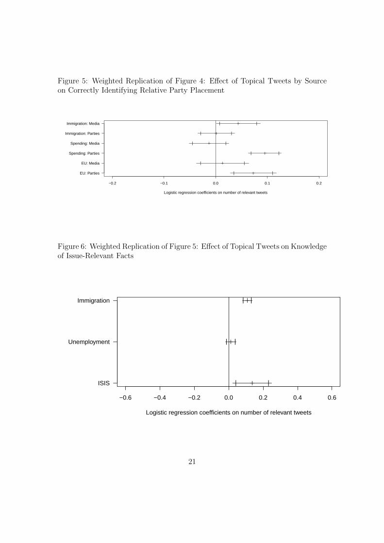
Figure 5: Weighted Replication of Figure 4: Effect of Topical Tweets by Sourceon Correctly Identifying Relative Party Placement
−0.2 −0.1 0.0 0.1 0.2
Logistic regression coefficients on number of relevant tweets
EU: Parties
EU: Media
Spending: Parties
Spending: Media
Immigration: Parties
Immigration: Media
|
|
|
|
|
|
|
|
|
|
|
|
Figure 6: Weighted Replication of Figure 5: Effect of Topical Tweets on Knowledgeof Issue-Relevant Facts
−0.6 −0.4 −0.2 0.0 0.2 0.4 0.6
Logistic regression coefficients on number of relevant tweets
ISIS
Unemployment
Immigration
|
|
|
|
|
|
21
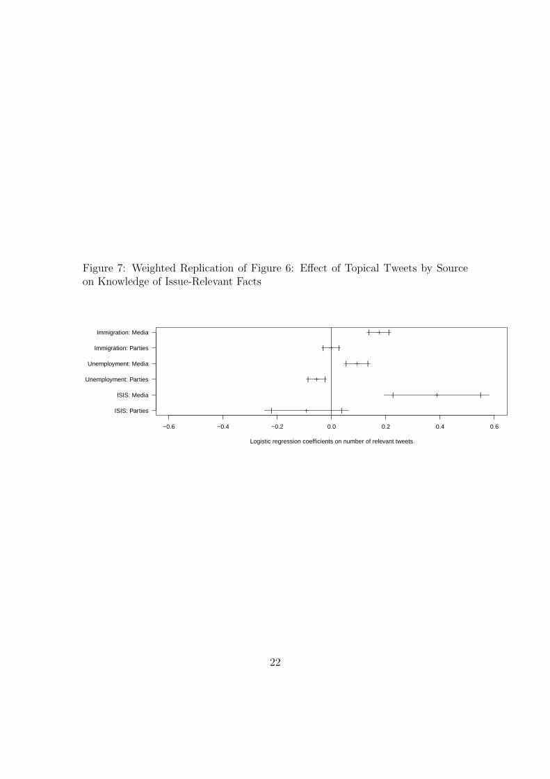
Figure 7: Weighted Replication of Figure 6: Effect of Topical Tweets by Sourceon Knowledge of Issue-Relevant Facts
−0.6 −0.4 −0.2 0.0 0.2 0.4 0.6
Logistic regression coefficients on number of relevant tweets
ISIS: Parties
ISIS: Media
Unemployment: Parties
Unemployment: Media
Immigration: Parties
Immigration: Media
|
|
|
|
|
|
|
|
|
|
|
|
22
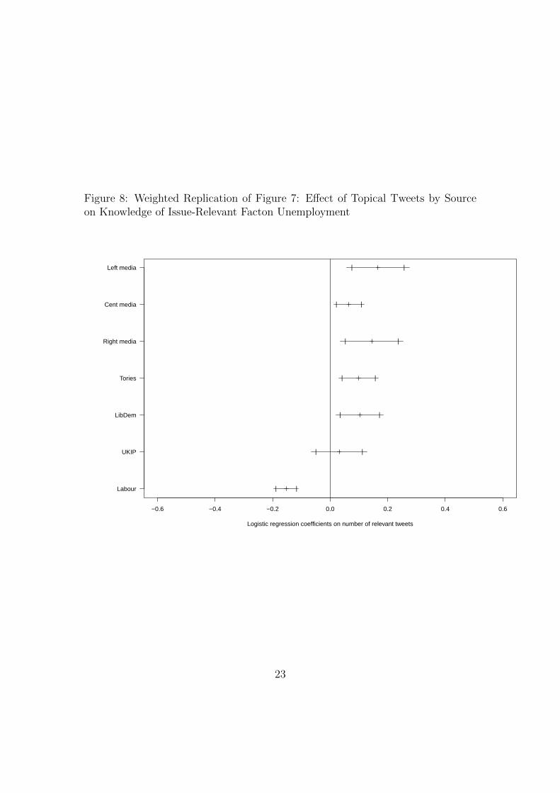
Figure 8: Weighted Replication of Figure 7: Effect of Topical Tweets by Sourceon Knowledge of Issue-Relevant Facton Unemployment
−0.6 −0.4 −0.2 0.0 0.2 0.4 0.6
Logistic regression coefficients on number of relevant tweets
Labour
UKIP
LibDem
Tories
Right media
Cent media
Left media
|
|
|
|
|
|
|
|
|
|
|
|
|
|
23
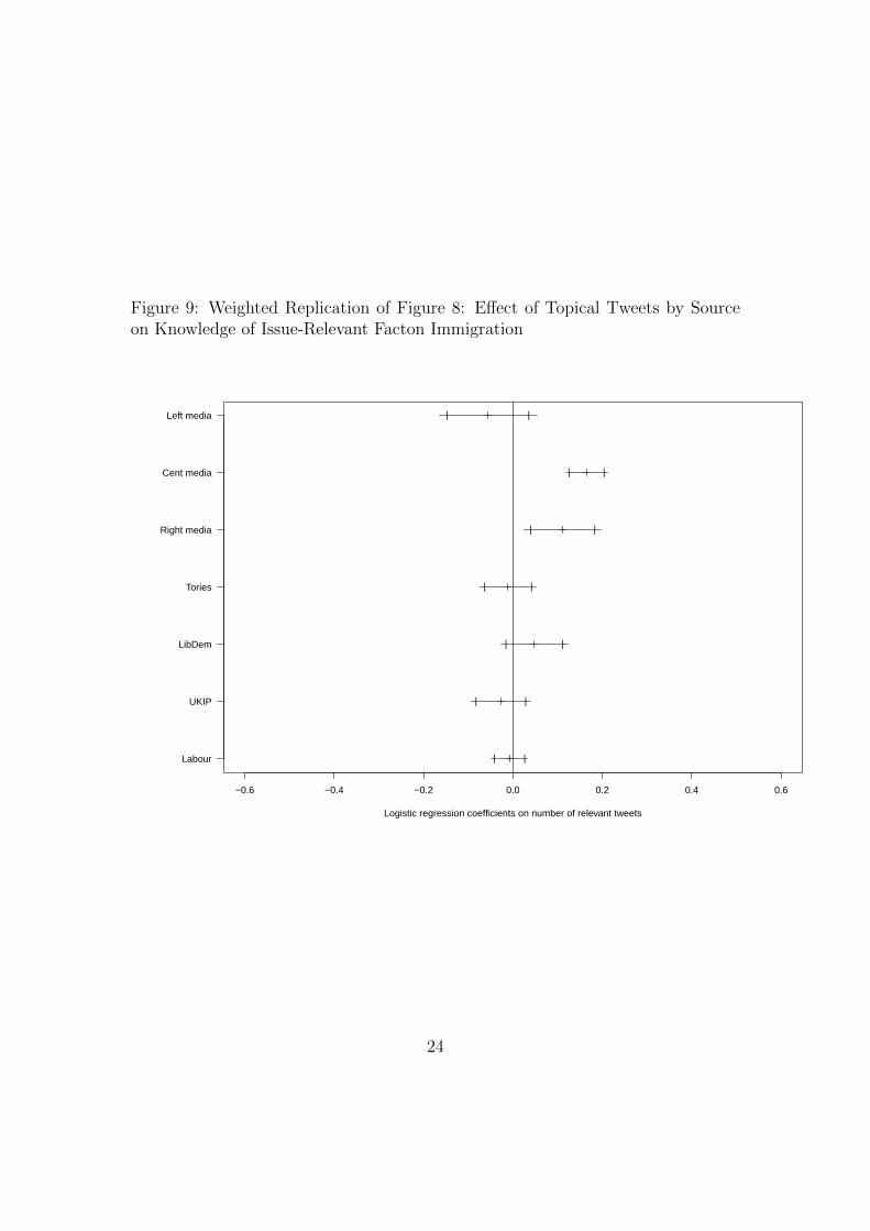
Figure 9: Weighted Replication of Figure 8: Effect of Topical Tweets by Sourceon Knowledge of Issue-Relevant Facton Immigration
−0.6 −0.4 −0.2 0.0 0.2 0.4 0.6
Logistic regression coefficients on number of relevant tweets
Labour
UKIP
LibDem
Tories
Right media
Cent media
Left media
|
|
|
|
|
|
|
|
|
|
|
|
|
|
24
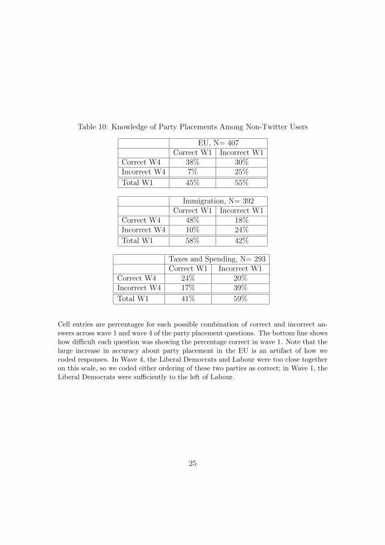
Table 10: Knowledge of Party Placements Among Non-Twitter Users
EU, N= 407Correct W1 Incorrect W1
Correct W4 38% 30%Incorrect W4 7% 25%
Total W1 45% 55%
Immigration, N= 392Correct W1 Incorrect W1
Correct W4 48% 18%Incorrect W4 10% 24%
Total W1 58% 42%
Taxes and Spending, N= 293Correct W1 Incorrect W1
Correct W4 24% 20%Incorrect W4 17% 39%
Total W1 41% 59%
Cell entries are percentages for each possible combination of correct and incorrect an-swers across wave 1 and wave 4 of the party placement questions. The bottom line showshow difficult each question was showing the percentage correct in wave 1. Note that thelarge increase in accuracy about party placement in the EU is an artifact of how wecoded responses. In Wave 4, the Liberal Democrats and Labour were too close togetheron this scale, so we coded either ordering of these two parties as correct; in Wave 1, theLiberal Democrats were sufficiently to the left of Labour.
25