
POLITECNICO DI MILANO · Politecnico di Milano for their support both ... simulando 5 cicli di...
207
POLITECNICO DI MILANO Scuola di Ingegneria Industriale e dell’Informazione Corso di Laurea in Ingegneria Meccanica Development and implementation in Amesim ® of the Model Predictive Control for the energy management of a HEV Relatore: Prof. MAPELLI Ferdinando Luigi Tesi di Laurea di: DONI Diego Matr.783101 Anno Accademico 2013-2014
-
Upload
truongquynh -
Category
Documents
-
view
213 -
download
1
Transcript of POLITECNICO DI MILANO · Politecnico di Milano for their support both ... simulando 5 cicli di...

POLITECNICO DI MILANO
Scuola di Ingegneria Industriale e
dell’Informazione
Corso di Laurea in
Ingegneria Meccanica
Development and implementation in Amesim
® of the Model
Predictive Control for the energy management of a HEV
Relatore: Prof. MAPELLI Ferdinando Luigi
Tesi di Laurea di:
DONI Diego Matr.783101
Anno Accademico 2013-2014


Acknowledgment
This thesis work marks the end of my university education which has been
tough, long but awesome. Studying in Milan and Stockholm, carrying out the
thesis at LMS Imagine in Lyon were great experiences and some people have
had a crucial role to make it possible. For this and for other reasons, I would like
to thank professor Annika Stensson Trigell from KTH, Royal Institute of
Technology and professors Federico Cheli, Ferdinando Luigi Mapelli from
Politecnico di Milano for their support both during the development of the work
and to write this report. Their nice suggestions made me understand that the
work was evolving in a good manner. They also encouraged me to analyze
interesting topics which made the thesis project even more interesting and
helped me to define a good layout for this report.
Let me thank all people I met at LMS Imagine in Lyon who were always kind,
friendly and warm with me. They involved me in many activities which made
me feel part of the company and made my time in France happier. Last but not
least a special thank goes to Yerlan Akhmetov and Bruno Lecointre from LMS
Imagine for the invaluable help and knowledge they gave me throughout my
staying in Lyon, and Peter Mas from LMS Imagine who decided to hire me as
intern.


...En del av mitt hjärta ligger där
och mina tankar flyger alltid dit...


Abstract
The rising price of fuel and the ever-restricting legislations on fuel consumption
and amount of pollutant emissions have encouraged almost all automotive
manufacturers to look for alternative propulsion systems which may replace the
well-established internal combustion engine. Hybridization seems the most
promising solution at least in the short term period. The term hybrid electric
vehicle indicates a ground vehicle which is equipped with either one or two
electric machines in addition to a conventional internal combustion engine. A
hybrid electric vehicle guarantees a great flexibility in the energy management
since both fuel energy and electric energy stored in a battery can be used
together to provide the necessary traction effort; however the superior operating
flexibility of the powertrain requires a complex control strategy which manages
efficiently the power flow among the components of the powertrain. In addition
hybrid vehicles establish new challenges for the designers in particular
considering the passengers’ quality perception of the vehicle, i.e. NVH (i.e.
Noise and Vibration Harshness). This thesis develops a MPC-based control
strategy for the energy management problem of a power-split hybrid electric
vehicle where fuel economy and reduction of the discomfort felt by passengers
during engine starting and stopping are the core objectives. The strategy is
formulated according to an optimization problem driven by the two objectives
above mentioned and subjected to multiple constraints. The constraints are
related to the operating points of the machines, to the need of assuring charge
sustenance of the vehicle and reduce the longitudinal oscillations due to engine
start and stop. The strategy has been validated over some standard drive cycles
and the performance have been compared to those achievable with a rule based
strategy. The thesis assesses the potential of implementing additional
information provided by interactive navigation systems like GPS and GIS in the
optimization problem; moreover it investigates which parameters affect the most
the numeric optimization. The results show a decrease in fuel consumption in all
standard drive cycles in comparison to the rule based strategy. The MPC-based
control strategy shows good robustness against vehicle parameters uncertainty
nonetheless the analysis has highlighted few weaknesses of the linear MPC
approach. All simulations have been carried out via co-simulation between
Simulink® and Amesim
®.
Keywords: model predictive control, power-split hybrid electric vehicle, energy
management.

Sommario
Il crescente costo del carburante e l’introduzione di leggi restrittive in materia di
consumo di combustibile ed emissione di sostanze nocive, sta spingendo i
costruttori mondiali di veicoli terrestri allo sviluppo di sistemi di propulsione
alternativi al consolidato motore a combustione interna. Nell’ultimo ventennio
varie sono state le soluzioni ipotizzate, ciò nonostante l’ibridizzazione sembra
attualmente la soluzione tecnica più promettente per raggiungere i traguardi di
superiore efficienza energetica. Un veicolo elettrico ibrido é equipaggiato con
un motore a combustione interna supportato da almeno un motore elettrico e da
una fonte di potenza elettrica. Grazie alla possibilità di utilizzare
contemporaneamente l’energia chimica del combustibile e l’energia elettrica
immagazzinata in una batteria ad alto voltaggio, i veicoli ibridi elettrici (HEV)
garantiscono elevata flessibilità operativa con potenzialità di ridurre in maniera
significativa le emissioni nocive e il consumo rispetto a un veicolo
convenzionale. Tuttavia la superiore efficienza energetica può essere raggiunta
solo a patto che tutti i componenti del sistema di propulsione cooperino in
sinergia. Questo richiede lo sviluppo di una strategia di controllo avanzata
capace di ottimizzare il flusso di potenza tra le macchine. In aggiunta gli HEVs
pongono nuove sfide nell’ambito della progettazione NVH dei veicoli. Questa
tesi ha l’obiettivo di sviluppare una strategia di controllo basata su Model
Predictive Control per la gestione del flusso di potenza del veicolo e la riduzione
delle vibrazioni del corpo vettura associate agli eventi di attivazione e
spegnimento del motore a combustione interna. La strategia risolve un problema
di ottimizzazione guidato dai due obiettivi menzionati in precedenza e soggetto
ai numerosi vincoli operativi delle macchine. La strategia é stata testata
simulando 5 cicli di guida standardizzati e le prestazioni in termini di riduzione
del consumo e delle vibrazioni del corpo vettura, sono state confrontate con
quelle ottenibili da una strategia concorrente basata su un approccio euristico.
La tesi analizza anche la potenzialità di integrare ulteriori informazioni rese
disponibili da sistemi di navigazione quali GPS e GIS nella gestione ottimale del
flusso di potenza. I risultati mostrano un decremento del consumo totale sui cicli
di guida standardizzati quando la strategia MPC é implementata; essa mostra
anche robustezza rispetto alla variabilità di alcuni parametri del veicolo e della
strada. Tuttavia emergono delle limitazioni dovute allo sviluppo di una strategia
linearizzata. Tutte le simulazioni sono state condotte in parallelo con i software
Simulink® e Amesim®.
Parole chiave: model predictive control, power-split hybrid electric vehicle,
energy management


Estratto in lingua italiana
Struttura della tesi
Questo lavoro di tesi ha lo scopo di sviluppare una strategia di controllo, basata
sull’approccio Model Predictive Control, del flusso di potenza nel sistema di
propulsione di un veicolo ibrido elettrico serie-parallelo, per migliorare
l’efficienza così da ridurre il consumo di carburante. L’intero lavoro é svolto al
calcolatore dove il veicolo di riferimento é rappresentato da un modello fisico-
matematico dettagliato implementato nel software commerciale Amesim®
distribuito da LMS International. Il progetto é stato interamente svolto presso
LMS International nella sede di Lione, Francia.
La tesi, scritta in lingua inglese, inquadra dapprima il problema di definire una
strategia di controllo per la gestione energetica di un veicolo ibrido elettrico,
successivamente descrive i passaggi matematici necessari per sviluppare la
strategia MPC. Nella terza parte vengono ampiamente discussi i risultati,
mettendo in luce vantaggi e svantaggi della strategia. La tesi é organizzata in
capitoli, in particolare i primi due capitoli inquadrano i veicoli ibridi elettrici nel
panorama dell’industria automobilistica attuale, evidenziando pregi e difetti
rispetto ad architetture concorrenti. Il terzo capitolo tratta in dettaglio
l’architettura serie-parallelo power split utilizzata in questa tesi, descrivendo i
componenti più importanti e le differenti modalità di guida. Il quarto capitolo
introduce e spiega la strategia di controllo MPC dal punto di vista
dell’ottimizzazione numerica necessaria per elaborare i comandi di controllo sul
sistema. Il quinto capitolo discute i risultati principali quelli cioè che pongono in
confronto le prestazioni della strategia MPC con quelle di una strategia
concorrente. Questo capitolo é importante in quanto chiarifica il principio
operativo della strategia. Il sesto capitolo affronta l’analisi in dettaglio dei
parametri che influenzano il funzionamento della strategia. É fatto largo uso
dell’analisi di sensibilità per estrarre informazioni utili circa la dipendenza delle
prestazioni della strategia dai valori dei parametri. L’ultimo capitolo conclude la
tesi riassumendo i punti principali e fornendo indicazioni su possibili sviluppi
futuri. Le tre appendici finali illustrano i passaggi matematici necessari per
implementare la strategia, eseguire l’analisi di sensibilità e i cicli di guida di
riferimento adottati in tutte le simulazioni numeriche.
L’ibrido come soluzione
Un terzo dell’intero consumo energetico mondiale é attribuito al trasporto di
merci e persone su gomma; ad esso si attribuisce anche una parte attiva nel
processo di riscaldamento dell’atmosfera terrestre. Per fronteggiare l’elevato
consumo energetico e ridurre l’emissione di sostanze inquinanti nell’atmosfera
sono state emanate leggi stringenti volte a incentivare il progresso tecnologico
Estratto in lingua italiana
II
nel campo automobilistico. Ad esempio l’unione europea ha fissato come
obiettivo per il 2020 il limite massimo di emissione di CO2 per gli autoveicoli
pari a 95g/km. Tutti i costruttori mondiali di autoveicoli stanno lavorando
instancabilmente alla ricerca di tecnologie innovative e soluzioni costruttive
capaci di ridurre il consumo e i tassi di emissione di inquinanti dei veicoli
stradali. Queste due problematiche sono principalmente collegate all’utilizzo di
un motore a combustione interna per generare la necessaria potenza e coppia di
propulsione. Per ridurre il consumo é necessario migliorare l’efficienza del
processo di combustione; allo stesso modo l’abbattimento dei tassi di emissione
di inquinanti é legato al trattamento dei prodotti della reazione chimica di
combustione. Nonostante la ricerca nell’ambito dei motori a combustione
interna abbia portato a notevoli progressi, é difficile pensare che in futuro sarà
possibile rispettare gli obiettivi sempre più stringenti avendo come unica leva lo
sviluppo del motore endotermico.
Per questa ragione nell’ultimo ventennio i costruttori automobilistici hanno
cercato alternative alla sola propulsione fornita dal motore a combustione
interna. La via privilegiata é quella dell’elettrificazione dove il sistema di
propulsione del veicolo si arricchisce di componenti elettromeccanici che hanno
lo scopo di affiancare o addirittura sostituire completamente il motore a
combustione interna nella generazione di potenza al fine di ridurre l’impatto
ambientale del veicolo. Le principali soluzioni proposte si distinguono in due
classi: quella dei veicoli completamente elettrici e quella dei veicoli ibridi. Nel
primo caso l’energia elettrica, ottenuta dalla conversione di energia chimica
immagazzinata in una batteria, é l‘unica fonte energetica del sistema che utilizza
un motore elettrico per la conversione di quest’ultima in potenza meccanica utile
alla propulsione. Nei veicoli ibridi elettrici invece il motore a combustione
interna é utilizzato in sinergia con uno o più motori elettrici al fine di
raggiungere una efficienza superiore rispetto a veicoli convenzionali e quindi
minor consumo e riduzione dei tassi di emissione di inquinanti. Il bilancio
energetico vede in questo caso due fonti primarie di energia rappresentate
dall’energia chimica immagazzinata in una batteria ad alto voltaggio e l’energia
chimica di un combustibile fossile. Grazie a queste due fonti energetiche
distinte, i veicoli ibridi elettrici non soffrono dei tipici problemi che affliggono i
veicolo elettrici e.g. limitata autonomia di guida data dalla ridotta capacità
elettrica delle batterie, lunghi periodi di ricarica della batteria. I veicoli elettrici
ibridi rappresentano dunque al giorno d’oggi la sola reale alternativa alla
propulsione basata interamente su un motore a combustione interna. Essi
pongono una grande sfida ingegneristica perché se da un lato la presenza
contemporanea di un motore endotermico e di macchine elettriche, insieme a
tutti i sottosistemi necessari al loro funzionamento e alla loro regolazione, rende
l’architettura della trasmissione e del sistema di propulsione assai complessa, da
un altro punto di vista la propulsione elettrica introduce un grado di libertà
III
aggiuntivo nel bilancio energetico del veicolo e la maggiore flessibilità nella
suddivisione del carico tra motore endotermico e macchine elettriche in base alle
condizioni operative. La suddivisione della potenza nei due rami del sistema di
propulsione é generalmente guidata da opportuni obiettivi che devono essere
raggiunti lungo una missione di guida. Tipicamente la riduzione del consumo
totale di combustibile e dei tassi di emissione istantanei di sostanze inquinanti
rappresentano due obiettivi della gestione energetica di un veicolo ibrido. In
parallelo occorre tenere conto dei molteplici vincoli esistenti sui punti di
funzionamento dei componenti pertanto la definizione di una corretta
ripartizione della generazione di potenza si riflette nella risoluzione di un
problema di ottimizzazione vincolata. Questo problema é indicato con il termine
energy management.
Il problema di ottimo
Data la complessità del problema, é richiesto lo sviluppo e l’implementazione di
una strategia di controllo che coordini le funzioni di tutte le macchine preposte
alla generazione di potenza meccanica al fine di raggiungere gli obiettivi
rispettando tutti i vincoli operativi. Il controllo é organizzato a livelli. Ogni
sottosistema (trasmissione, batteria, motore endotermico, macchine elettriche) é
gestito da un suo controllore che imposta il punto di funzionamento della
macchina in base alle istruzioni ricevute; tali controllori sono definiti di basso
livello. Al livello più alto é posto l’autista che fornisce i comandi base tramite i
pedali di acceleratore e freno ed eventualmente tramite il cambio marcia.
L’interazione della struttura di controllo con altre logiche di controllo (ABS,
ESP etc...) é gestita da una controllore di alto livello posto appena sotto l’autista
sulla scala gerarchica. Il cuore della strategia é però il Vehicle Supervisory
Controller. Questo elemento implementa la vera strategia di controllo del flusso
di potenza; esso riceve le informazioni dai sensori e le specifiche dall’autista e
interagisce con i controllori di basso livello per coordinare il funzionamento di
tutte le macchine. La grande sfida consiste nel definire questa strategia di
controllo e gli approcci finora sperimentati si racchiudono in due classi:
Strategie rule based: sfruttando le informazioni fornite da vari sensori, il
controllore riconosce lo stato di funzionamento del veicolo. Per ogni
stato di funzionamento la strategia dispone di delle azioni di controllo
reimpostate che vengono automaticamente applicate al sistema.
Strategie di controllo ottimo: il rapporto di suddivisione della potenza
tra motore endotermico e propulsione elettrica é il risultato di un
problema di ottimizzazione. Questa classe é ulteriormente suddivisa in
metodologie globali e locali, dove la denominazione é basata sulla
lunghezza dell’orizzonte temporale futuro che viene considerato nel
problema di ottimizzazione.
Estratto in lingua italiana
IV
Data la natura statica delle strategie rule based, le azioni di controllo non sono
ottimali per la particolare situazione di guida quindi il veicolo non lavora in
genere nelle migliori condizioni di efficienza. Queste tecniche sono però le più
semplici da implementare perché non sono computazionalmente dispendiose. Le
tecniche di ottimizzazione globali quali Dynamic Programming assumono di
conoscere in anticipo l’esatto profilo di potenza richiesta lungo tutta la missione
di guida pertanto riescono a calcolare off line l’azione di controllo valida per
tutta la missione. Nei casi in cui non intervengano perturbazioni esterne la
strategia risulta essere la migliore in assoluto. Nella realtà é però impossibile
conoscere con esattezza il profilo futuro di potenza richiesta pertanto queste
strategie sono per lo più utilizzate nell’ambito della simulazione numerica per
fornire la soluzione di riferimento, le cui prestazioni servono da metro di
giudizio rispetto alle strategie real time, in modo da capire le effettive
potenzialità del controllore sviluppato. Dal punto di vista dell’implementazione
real time le strategie di ottimizzazione locale sono più interessanti. Esse limitano
l’ottimizzazione a pochi istanti futuri cercando di prevedere l’evoluzione della
richiesta di potenza, oppure limitano il problema di ottimo all’istante di
campionamento. Model Predictive Control é un esempio del primo approccio
invece A-ECMS é un esponente del secondo.
Questa tesi affronta la definizione di una strategia di controllo basata su Model
Predictive Control per il problema energetico di un veicolo ibrido elettrico serie-
parallelo power split. Questo tipo di ibrido garantisce la maggior flessibilità
nella gestione della produzione di potenza, quindi é candidato a fornire la
migliore evoluzione rispetto a un veicolo convenzionale motorizzato da un solo
motore a combustione interna. Il Model Predictive Control é un metodo che
elabora una strategia di controllo per un sistema dinamico che sia ottima rispetto
a una funzione di merito e che soddisfi tutti i vincoli operativi agenti sul sistema.
Il metodo MPC utilizza un modello di riferimento della dinamica del sistema per
prevedere la sua risposta ad ingressi noti di controllo e di disturbo esterno lungo
un orizzonte di previsione futuro. I soli valori di controllo che portano il sistema
a soddisfare tutti i vincoli operativi lungo l’orizzonte di previsione sono presi in
considerazione e tra questi si estraggono unicamente quelli che rendono ottima
la funzione di merito lungo lo stesso orizzonte di previsione. MPC é già
applicato con successo nell’industria chimica, a cui deve la sua nascita, ma
grazie all’evoluzione nel campo dei microprocessori sta crescendo il suo
impiego in ambito automobilistico. La decisione di applicare il metodo MPC per
lo sviluppo di una strategia di controllo di alto livello nasce dalla forza di tale
metodo di includere molteplici vincoli operativi già nella risoluzione del
problema di ottimo, dunque la strategia rispetta i vincoli e può essere
direttamente applicata al sistema. In più la natura previsionale del metodo
suggerisce che l’adozione di sistemi di navigazione quali GPS, informazioni sul

V
traffico etc.. possano migliorare la previsione della potenza richiesta in futuro
dall’autista e quindi l’efficienza del veicolo.
Sviluppo della strategia MPC
Il metodo MPC é basato su 4 punti cardine:
Modello di riferimento della risposta del sistema a ingressi noti
Funzioni di vincolo
Funzione di merito
Ottimizzazione numerica
Come descritto brevemente in precedenza, il metodo MPC calcola i valori delle
variabili di controllo da applicare al sistema all’istante immediatamente
successivo a quello di campionamento basandosi sulla risoluzione di un
problema di ottimizzazione. Il metodo utilizza le condizioni misurate all’istante
di campionamento e un modello affidabile della risposta del sistema per
prevedere la sua evoluzione lungo un orizzonte futuro di previsione sotto la
guida di una sequenza di controlli. Esistono diverse possibili sequenze di
controlli che possono portare il sistema dalle condizioni iniziali a quelle finali
desiderate rispettando tutti i vincoli operativi; tuttavia esiste solo una sequenza
che, svolgendo tale compito, rende ottima una funzione di merito assegnata.
MPC risolve quindi un problema di ottimizzazione per calcolare questa sola
sequenza ottima. Nella formulazione classica del metodo MPC la sequenza di
controllo è applicata lungo un orizzonte di controllo futuro di lunghezza uguale
o inferiore rispetto all’orizzonte di previsione. Dunque MPC risolve un
problema di ottimizzazione basato sull’evoluzione futura del sistema, tuttavia
esso applica solo i valori di controllo che corrispondono al primo passo di
evoluzione andando poi a ripetere l’intero processo di ottimizzazione servendosi
delle nuove informazioni disponibili al successivo campionamento e spostando
in avanti di un passo l’orizzonte di previsione. Questa tecnica di calcolo
ricorsiva prende il nome di receding horizon e porta a definire un controllo in
retroazione.
Una delle problematiche dell’ottimizzazione numerica sta nel assicurare che
l’algoritmo converga a un punto di ottimo del sistema e che tale punto sia
l’ottimo globale. Qualora il problema godesse della proprietà di convessità
allora esisterebbe un solo punto di ottimo e questo sarebbe di ottimo globale. É
possibile garantire questa proprietà definendo il problema secondo la forma
canonica della programmazione quadratica cioè con funzione di merito
quadratica nelle variabili di progetto, i.e. le variabili di controllo, e definita
positiva mentre i vincoli devono essere espressi sotto forma di disuguaglianze
lineari. I quattro punti elencati in precedenza sono implementati numericamente

Estratto in lingua italiana
VI
cercando di rispettare queste condizioni per la convessità del problema di
ottimizzazione; di seguito si fornisce una breve descrizione dei passaggi
matematici che si rendono necessari.
Il modello di riferimento
Il veicolo analizzato in questa tesi é un ibrido elettrico serie-parallelo di tipo
power split che non riflette nello specifico nessun veicolo reale. Lo scopo non é
infatti quello di ottimizzare un veicolo specifico ma piuttosto sviluppare una
strategia di controllo e valutarne le potenzialità. Si é utilizzato come riferimento
un modello dettagliato implementato nel software Amesim® che consente di
riprodurre la dinamica longitudinale del veicolo e il funzionamento dei suoi
componenti principali quali motore a combustione interna, macchine elettriche,
batteria ad alto voltaggio e trasmissione. In più il modello consente di eseguire
analisi di base sul comfort limitate al campo di bassa frequenza e ai moti di
beccheggio e scuotimento verticale della cassa. Il modello é costruito a blocchi
dove ogni blocco descrive il comportamento di un componente mediante
equazioni matematiche. Lo schema costruttivo del veicolo é rappresentato nella
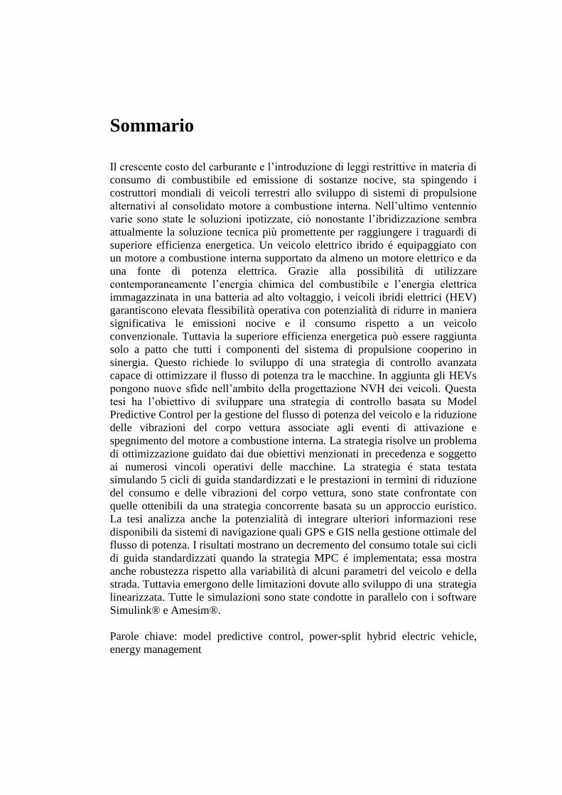
prossima figura.
Figura 1: Sistema di propulsione di un ibrido elettrico power-split.
Un veicolo ibrido elettrico power split si compone di un motore endotermico e
due macchine elettriche collegate a un rotismo epicicloidale (power splite
device) che ha la scopo di ripartire la potenza tra queste tre macchine e la sala
motrice anteriore. Le due macchine elettriche possono operare sia da motore che
da generatore e definiscono il carico per la batteria ad alto voltaggio posta sulla
sala posteriore. La power control unit é l’elettronica di potenza che, sulla base
della strategia di controllo implementata al suo interno, fissa la ripartizione e il
flusso di potenza tra motore endotermico e batteria elettrica in modo tale da
bilanciare le richieste dell’autista e rispettare i vincoli operativi del veicolo.
Grazie al rotismo epicicloidale e alla batteria ad alto voltaggio é consuetudine
affermare che un ibrido power split ha due gradi di libertà nella gestione della

VII
potenza. Tramite il rotismo epicicloidale la velocità angolare dell’albero a
gomiti é indipendente dalla velocità angolare delle ruote motrici consentendo di
fissare liberamente la velocità angolare del motore endotermico e quindi dando
un notevole vantaggio in termini di efficienza energetica. In più la batteria ad
alto voltaggio funge da buffer energetico assorbendo l’eccesso di potenza
prodotta dal motore endotermico rispetto a quanto richiesto alla ruota e fornendo
invece potenza alle ruote motrici quando la potenza prodotta dal motore termico
non é sufficiente. Questo si traduce in un ulteriore vantaggio in termini di
efficienza energetica perché nelle condizioni di bassa richiesta di potenza il
motore termico può produrre un surplus di potenza in condizioni di alta
efficienza che viene immagazzinata nella batteria e riutilizzata nelle fasi di
massima richiesta di potenza, andando così a supportare il motore endotermico
che pertanto non deve pareggiare il carico massimo e può mantenere un punto
operativo caratterizzato da basso consumo. Quanto descritto si attua tramite una
opportuna strategia di controllo che utilizza il generatore elettrico e il rotismo
epicicloidale per governare il punto di funzionamento del motore a combustione
interna; dato che la velocità angolare dell’albero a gomiti può essere settata in
maniera indipendente rispetto alla velocità angolare delle ruote motrici si suole
indicare il gruppo rotismo epicicloidale - generatore elettrico come una e-CVT
(electronic continuous variable transmission). Un veicolo di questo tipo dispone
di numerose modalità di guida che spaziano da una modalità totalmente
elettrica, alla modalità power-split dove motore endotermico e batteria
cooperano per raggiungere la migliore efficienza energetica, alla modalità
parallela dove tutta la potenza prodotta dal motore termico fluisce alle ruote
motrici, alla frenata rigenerativa che rappresenta un’ulteriore guadagno in
termini di efficienza energetica visto che parte dell’energia cinetica del veicolo é
impiegata per ricaricare la batteria senza utilizzare parte della potenza prodotta
dal motore a combustione interna. La sala motrice anteriore é collegata
all’albero che reca la corona del rotismo epicicloidale e il rotore del motore
elettrico tramite una cinghia non riportata nella figura precedente.
Il modello implementato in Amesim® consente di modellare tutte queste fasi di
guida, tuttavia esso é troppo complesso per poter essere utilizzato come
riferimento da MPC per prevedere la risposta del sistema eseguendo numerose
valutazioni in poco tempo. Di conseguenza si é provveduto a estrarre un
modello matematico più semplice in grado di cogliere gli aspetti fondamentali
del problema energetico tralasciando quelli meno importanti. I seguenti
componenti sono stati modellati:
Motore a combustione interna
Macchine elettriche
Trasmissione
Batteria ad alto voltaggio

Estratto in lingua italiana
VIII
La dinamica dell’albero a gomiti e l’andamento dello stato di carica della
batteria sono stati modellati mediante due equazioni differenziali del primo
ordine, invece tutti gli altri componenti sono stati descritti tramite una
modellazione quasi statica. Il funzionamento della batteria ad alto voltaggio é
stato descritto secondo il modello di un circuito elettrico equivalente come
rappresentato nella prossima figura:
dove corrisponde al voltaggio di circuito aperto della batteria,
corrisponde alla resistenza interna equivalente della batteria, e rappresentano rispettivamente il voltaggio e la corrente ai morsetti della batteria.
Lo derivata temporale dello stato di carica della batteria é definita dalla seguente
equazione differenziale:
(1)
dove indica lo stato di carica della batteria, é la variabile temporale,
é la capacità elettrica della batteria, é la potenza totale scambiata dalla
batteria con le macchine elettriche. La potenza della batteria funge da
collegamento con il sistema di propulsione, comprensivo del motore
endotermico, delle macchine elettriche e della trasmissione alle ruote motrici.
Esso é schematizzato come segue:
Engine Generator
Motor
Te
Tc
Tr Tr
Ts
Tg
Tm
Tout
Tout Tb
Froad
Je

IX
dove rappresenta l’inerzia rotazionale del volano, la coppia del motore
endotermico all’albero, la velocità angolare dell’albero a gomiti, la coppia
del planetario, la velocità angolare del planetario, la coppia del solare,
la velocità angolare del solare, la coppia della corona, la velocità angolare
della corona, la coppia del generatore al rotore, la velocità angolare del
rotore del generatore, la coppia del motore elettrico al rotore, la velocità
angolare del rotore del motore elettrico, il rapporto di trasmissione totale tra
corona e ruote motrici, la velocità angolare delle ruote motrici, la
coppia totale all’uscita o in ingresso alla trasmissione, la totale coppia
frenante applicata dal sistema frenante di servizio, la totale forza resistente
esercitata dalla spinta aerodinamica e dalla resistenza al rotolamento. La
dinamica longitudinale del veicolo é schematizzata servendosi dell’analogia del
moto di avanzamento di un punto materiale soggetto alla forza di trazione e alle
forze resistive date dalla resistenza al rotolamento e dalla spinta aerodinamica.
La componente della forza peso parallela al terreno é stata trascurata in quanto si
é assunto nella prima parte di questa tesi che la strategia di controllo non possa
conoscere la pendenza della strada. Assumendo nota la coppia totale alle ruote
richiesta dall’autista, definita come:
(2)
é possibile integrare la velocità di avanzamento del veicolo lungo un orizzonte
temporale a partire dalla equazione differenziale che governa la
dinamica longitudinale del veicolo.
(3)
dove indica la ierzia equivalente del veicolo comprensiva del corpo vettura e
di tutti gli organi in moto, é il grado di avanzamento del veicolo, la
densità dell’aria, il coefficiente adimensionale di resistenza aerodinamica,
la massa del veicolo, l’accelerazione di gravità, il coefficiente di resistenza
al rotolamento, il raggio di rotolamento della ruota.
Dalla conoscenza della coppia e della velocità si ricava il profilo della potenza
richiesta dall’autista lungo l’orizzonte temporale . Noto questo profilo
in ingresso, è compito della strategia di controllo decidere come utilizzare la
potenza prodotta dal motore endotermico e dalle macchine elettriche per
bilanciarlo. Siano la coppia all’albero fornita dal motore endotermico, la coppia
del generatore elettrico e la totale coppia frenante prodotta dal sistema frenante

Estratto in lingua italiana
X
di servizio le variabili di controllo del sistema; siano la velocità di avanzamento
del veicolo e la coppia totale richiesta dall’autista gli ingressi misurati. Tramite
queste grandezze è possibile descrivere il funzionamento di tutti i componenti
del sistema di propulsione. Le equazioni fondamentali sono riportate di seguito:
(4)
con ad indicare il numero di denti della corona e del solare.
Assumendo la velocità angolare dell’albero a gomiti e lo stato di carica della
batteria come stati del sistema, si ricava la forma di stato non lineare che
caratterizza il comportamento del sistema:
(5)
dove:
contiene gli stati del sistema, le variabili di controllo mentre le variabili
esterne misurate.
Nonostante ai fini dello sviluppo di una strategia di controllo per lo energy
management di un veicolo ibrido sia sufficiente considerare solo la dinamica

XI
dello stato di carica della batteria in quanto tutte le altre dinamiche del sistema
sono molto più veloci, in questo modello viene anche descritta la dinamica
dell’albero a gomiti in quanto si vuole utilizzare la strategia stessa per addolcire
l’intervento del generatore elettrico nelle fasi di attivazione e spegnimento del
motore endotermico così da ridurre il discomfort patito dai passeggeri. Lo scopo
è sviluppare una strategia di controllo che incorpori anche alcuni obiettivi
riguardanti il comfort a bordo e dunque non richieda delle modifiche ulteriori
per poter essere applicata al veicolo.
Per definire completamente la forma di stato non lineare occorre determinare le
espressioni analitiche delle funzioni e . In particolare é necessario
ricavare un modello di regressione del consumo istantaneo di combustibile
rispetto alla variabile di controllo e allo stato , esprimere le perdite di
potenza nelle macchine elettriche rispetto a e la resistenza interna della
batteria ad alto voltaggio come funzione dello stato . Tutte queste relazioni
sono reperibili in Amesim® sotto forma di tabella multi ingresso, non
direttamente utilizzabili da un algoritmo numerico per la risoluzione del
problema di ottimizzazione. É necessario dunque sostituire tali tabelle con
modelli di regressione polinomiale; di seguito sono riportati i modelli di
regressione utilizzati.
Il consumo istantaneo di combustibile [kg/s] é espresso come funzione della
coppia [Nm] erogata dal motore a combustione interna e la velocità angolare
[rad/s] dell’albero a gomiti secondo la relazione seguente:
(6)
I coefficienti del polinomio valgono:
Tabella 1: Coefficienti di regressione polinomiale del consumo di combustibile.
Coefficiente Valore

Estratto in lingua italiana
XII
La potenza persa nelle macchine elettriche, espressa in W, é legata alla coppia
erogata dalla macchina [Nm] e alla velocità angolare del rotore [rad/s] dalla
seguente relazione:
(7)
Da ultima, la resistenza interna [Ω] di una singola cella della batteria é espressa
in funzione dello stato di scarica della batteria stessa [%]:
(8)
La resistenza interna equivalente della batteria si ricava conoscendo la
disposizione dei banchi di celle in serie e parallelo.
L’onere computazionale nell’utilizzare una forma di stato non lineare come
modello di riferimento per MPC è elevato, in più non è garantita la convessità
del problema di ottimizzazione. Di conseguenza la forma di stato è linearizzata
ad ogni istante di campionamento sfruttando ogni volta le nuove informazioni
rese disponibili dai sensori. La strategia MPC, dunque, utilizza la forma di stato
linearizzata per prevedere la risposta del sistema dalle condizioni definite
all’istante di campionamento fino al termine dell’orizzonte di previsione sotto
l’effetto degli ingressi misurati e delle variabili di controllo. Tale tecnica prende
il nome di LTV-MPC (Linear Time Varying). L’evoluzione della coppia totale
richiesta dall’autista è calcolata dalla strategia stessa secondo un andamento a
decadimento esponenziale a partire dal valore misurato all’istante di
campionamento mentre la velocità di avanzamento è ottenuta tramite
integrazione della dinamica longitudinale del veicolo. La forma di stato è
linearizzata secondo una serie di Taylor troncata al termine lineare:
(9)
con:
(10)
L’approccio canonico del metodo MPC è nel dominio discreto del tempo
pertanto la forma di stato linearizzata è discretizzata tramite Eulero avanti che
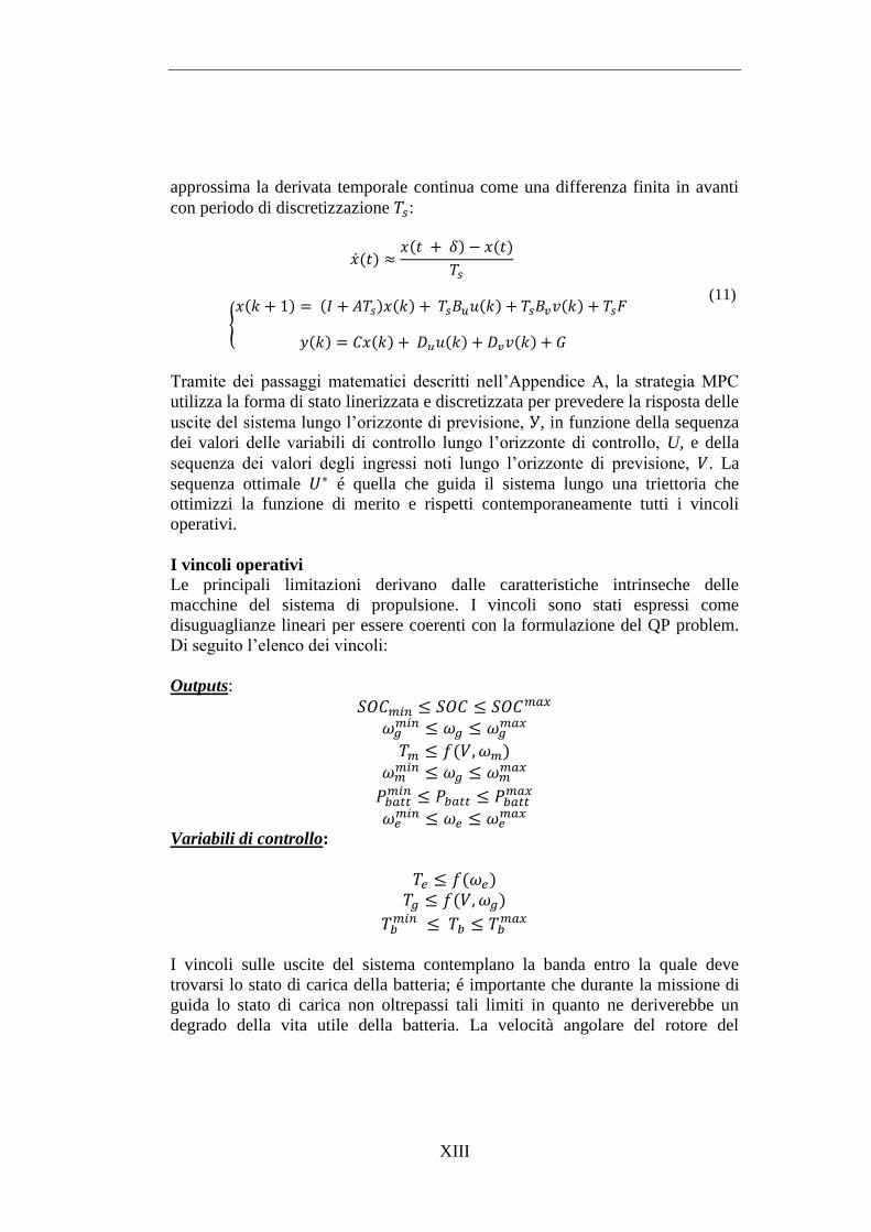
XIII
approssima la derivata temporale continua come una differenza finita in avanti
con periodo di discretizzazione :
(11)
Tramite dei passaggi matematici descritti nell’Appendice A, la strategia MPC
utilizza la forma di stato linerizzata e discretizzata per prevedere la risposta delle
uscite del sistema lungo l’orizzonte di previsione, , in funzione della sequenza
dei valori delle variabili di controllo lungo l’orizzonte di controllo, U, e della
sequenza dei valori degli ingressi noti lungo l’orizzonte di previsione, . La
sequenza ottimale é quella che guida il sistema lungo una triettoria che
ottimizzi la funzione di merito e rispetti contemporaneamente tutti i vincoli
operativi.
I vincoli operativi
Le principali limitazioni derivano dalle caratteristiche intrinseche delle
macchine del sistema di propulsione. I vincoli sono stati espressi come
disuguaglianze lineari per essere coerenti con la formulazione del QP problem.
Di seguito l’elenco dei vincoli:
Outputs:
Variabili di controllo:
I vincoli sulle uscite del sistema contemplano la banda entro la quale deve
trovarsi lo stato di carica della batteria; é importante che durante la missione di
guida lo stato di carica non oltrepassi tali limiti in quanto ne deriverebbe un
degrado della vita utile della batteria. La velocità angolare del rotore del
Estratto in lingua italiana
XIV
generatore elettrico deve essere compresa tra i due valori limite, lo stesso vale
per la velocità angolare del motore elettrico e i limiti superiore ed inferiore sono
identici essendo le due macchine elettriche uguali tra loro. La coppia massima
che il motore elettrico può produrre in funzione del voltaggio applicato alla
macchina e alla velocità angolare del rotore rappresenta un altro vincolo che
viene duplicato anche per valori negativi della coppia quando il motore opera
come generatore. Un ulteriore vincolo é rappresentato dalla massima potenza
prodotta ed assorbita dalla batteria ad alto voltaggio. Infine i limiti superiore ed
inferiore della velocità angolare dell’albero a gomiti chiudono i vincoli sulle
uscite del sistema. Per quanto riguarda i vincoli sulle variabili di controllo
vengono considerate le curve di coppia massima del motore a combustione
interna e del generatore elettrico espresse rispettivamente in funzione della
velocità angolare dell’albero a gomiti e della velocità angolare del rotore e del
voltaggio. Da ultimo la massima coppia frenante che il sistema frenante di
servizio é in grado di produrre alle ruote rappresenta il limite superiore per tale
coppia mentre la coppia nulla é il limite inferiore. Le curve caratteristiche di
coppia delle macchine sono fornite dal modello in Amesim®
; per poterle
implementare sotto forma di disuguaglianze lineari é necessario linearizzare le
curve tramite un’approssimazione lineare a tratti e prescrivere che la coppia
effettiva sia inferiore oppure superiore ad una data retta in funzione della
velocità angolare dell’albero. Grazie alle relazioni lineari é possibile raccogliere
i vincoli nella seguente forma matriciale:
(12)
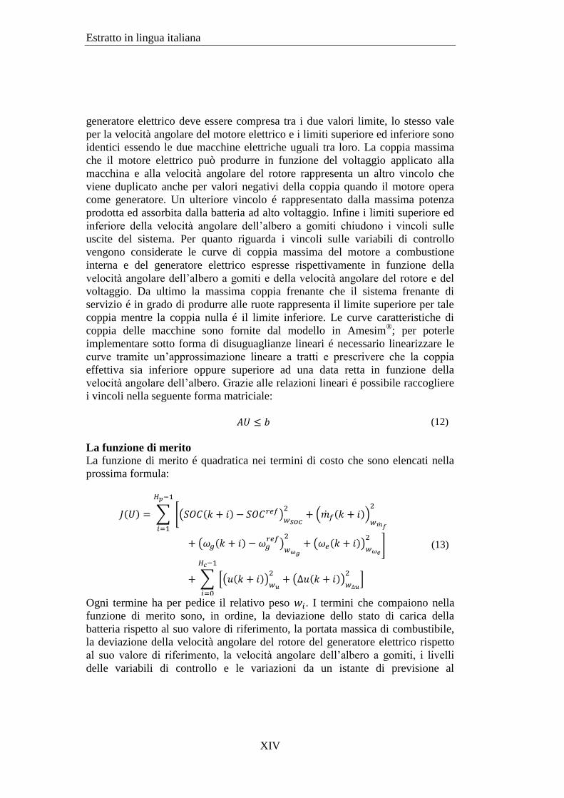
La funzione di merito
La funzione di merito é quadratica nei termini di costo che sono elencati nella
prossima formula:
(13)
Ogni termine ha per pedice il relativo peso . I termini che compaiono nella
funzione di merito sono, in ordine, la deviazione dello stato di carica della
batteria rispetto al suo valore di riferimento, la portata massica di combustibile,
la deviazione della velocità angolare del rotore del generatore elettrico rispetto
al suo valore di riferimento, la velocità angolare dell’albero a gomiti, i livelli
delle variabili di controllo e le variazioni da un istante di previsione al

XV
successivo delle variabili di controllo. I primi due termini governano il problema
energetico decretando la ripartizione di produzione di potenza tra batteria e
combustibile mentre tutti gli altri termini servono per migliorare la stabilità della
strategia oppure per migliorarne le prestazioni in particolare situazioni di guida e
sono stati aggiunti a seguito di numerose simulazioni preliminari che hanno
consentito la comprensione più approfondita del funzionamento della strategia.
La funzione di merito considera la somma dei quadrati dei termini su tutto
l’orizzonte di previsione per le uscite del sistema, mentre la somma é estesa a
tutto l’orizzonte di controllo per le variabili di controllo.
Sfruttando la notazione matriciale discreta della forma di stato é possibile
esplicitare le uscite del sistema in funzione dei livelli delle variabili di controllo
e in definitiva esprimere la funzione di merito come una funzione quadratica
nelle variabili di controllo.
(14)
dove raccoglie i termini costanti non importanti ai fini dell’ottimizzazione.
Algoritmo Active-set
Il problema di ottimizzazione vincolata é dunque formulato come un problema
di programmazione quadratica nella forma canonica:
soggetto a:
Le matrici e i vettori sono inizializzati a ogni istante di
campionamento sfruttando le informazioni misurate sul sistema. Il vettore
delle variabili di controllo che risolve il problema di ottimo é calcolato mediante
algoritmo active-set.
Risultati
Il modello dettagliato in Amesim® implementa una strategia di tipo rule based
per la gestione del flusso di potenza; scopo della strategia MPC é rimpiazzare
l’approccio euristico garantendo prestazioni superiori. La validazione della
strategia MPC é quindi stata condotta secondo i seguenti punti principali:
Valutazione del consumo totale del veicolo rispetto a cicli di guida
standardizzati di cui é nota la lunghezza, l’altimetria e la velocità
desiderata.

Estratto in lingua italiana
XVI
Confronto del consumo totale ottenuto dalle due strategie per ogni ciclo
di guida standard in condizioni di equilibrio energetico.
L’utilizzo di cicli di guida standardizzati consente di eliminare la variabilità
dello stile di guida dell’autista nella valutazione dei consumi. L’autista é
modellato mediante un regolatore PI sull’errore istantaneo tra la velocità
desiderata e la velocità attuale del veicolo, questo tipo di simulazione é detta “in
avanti” ed é molto utile per analizzare le prestazioni e la stabilità della strategia
di controllo. Al contrario un approccio “all’indietro” escluderebbe l’autista dal
modello assegnando direttamente il profilo di velocità desiderato e i calcoli
procederebbero a ritroso lungo il flusso di potenza per determinare le coppie
motrici necessarie a realizzare il moto. I cicli di guida standardizzati che sono
stati impiegati in questo lavoro di tesi sono NEDC, HWFET, UDDS, SC03,
US06; i loro profili di velocità desiderata sono riportati nell’Appendice C, la
quota altimetrica é sempre stata presa costante a 0 m su livello del mare.
Tutti i risultati fanno riferimento ad un veicolo in equilibrio energetico cioè il
livello finale dello stato di carica della batteria coincide con il livello iniziale. Il
veicolo preso in esame é classificato “a sostentamento di carica” dunque non é
prevista una fonte esterna di energia che ricarichi la batteria ad alto voltaggio ma
viene utilizzata parte della potenza prodotta dal motore endotermico per questo
scopo. Una valutazione del consumo nella situazione in cui livello iniziale e
finale dello stato di carica siano uguali é preferibile perché illustra
completamente la ripartizione del flusso di potenza tra le macchine. Per
raggiungere tale situazione é sufficiente ripetere la medesima missione di guida
aggiornando ogni volta il livello iniziale dello stato di carica con il livello finale
dell’ultima missione. L’analisi completa delle prestazioni della strategia MPC
ha cercato di coprire quanti più aspetti possibili che verranno ad uno ad uno
affrontati qui di seguito. É doveroso sottolineare come la strategia MPC
campiona le informazioni dai sensori di misura in maniera discreta con periodo
di campionamento pari a 0.1s, al contrario la strategia rule based lavora in
continuo campionando gli ingressi e aggiornando i valori delle variabili di
controllo ad ogni passo di integrazione numerica. Questo conferisce un piccolo
vantaggio alla strategia rule based mentre rende la strategia MPC più vicina ad
una reale applicazione.
Fuel economy
Dall’informazione sulla massa di combustibile consumato, si determina la fuel
economy tramite la relazione riportata di seguito.

XVII
(15)
dove corrisponde alla densità del combustibile liquido mentre distance
indica la distanza totale percorsa dal veicolo lungo la missione di guida
considerata.
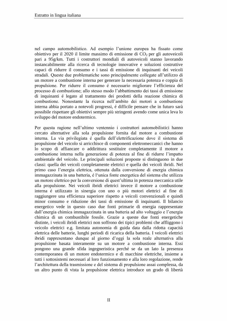
La prossima tabella e il prossimo istogramma illustrano le differenze tra le due
strategie in termini di efficienza energetica.
Tabella 2: Consumo di carburante ottenuto dalle due strategie sui 5 cicli di riferimento.
Rule based MPC
Cycle
NEDC 59.86 509.03 5.927 59.49 493.6 5.742
HWFET 59.65 751.25 5.837 59.73 741.62 5.762
SC03 47.97 286.47 6.378 57.34 261.16 5.815
UDDS 58.14 546.0 5.840 57.46 541.59 5.793
US06 42.00 901.59 8.973 56.17 741.53 7.380
Figura 2: Riduzione percentuale di consumo ottenuta con MPC rispetto alla strategia euristica.
Entrambe le strategie soddisfano tutti i vincoli operativi, unica eccezione la
strategia rule based che non riesce a mantenere il livello di carica della batteria
entro il limite inferiore sul ciclo US06. L’istogramma dimostra che la riduzione
percentuale di consumo totale ottenuta mediante MPC varia a seconda del ciclo
di guida, con risultati migliori per situazioni di guida extra-urbana caratterizzate
da alte velocità e alta richiesta di potenza. I cicli SC03 e US06 alternano brusche
accelerazioni a tratti di alta velocità dove la strategia di controllo é chiamata a
gestire il flusso di potenza in condizioni di alta richiesta di potenza su un
limitato periodo di tempo. Il ciclo UDDS rappresenta una condizione di guida

Estratto in lingua italiana
XVIII
urbana dove il vantaggio portato da MPC é risibile. La spiegazione a questi
risultati é da cercare nel principio operativo attuato da MPC.
Tale strategia sfrutta costantemente i gradi di libertà forniti da rotismo
epicicloidale e dal buffer di energia rappresentato dalla batteria ad alto
voltaggio. Un esempio lampante di questo comportamento é fornito dalle
prossime figure che mostrano alcuni risultati tratti dal ciclo autostradale
HWFET per le due strategie di controllo. Il tratto di ciclo a cui fanno riferimento
i risultati considera una prima parte di accelerazione in cui la velocità cresce
fino a superare i 90 km/h, seguita da un tratto a velocità pressoché costante. Il
profilo di velocità é riportato nella prossima figura.
Figura 3: Profilo di velocità nel tratto di guida considerato.
Le prossime due figure riportano il flusso di potenza attraverso il sistema di
propulsione per la strategia rule based a sinistra e per MPC a destra.
Figura 4: Bilancio di potenza ottenuto con
la strategia euristica.
Figura 5: Bilancio di potenza ottenuto con
MPC.

XIX
La strategia rule based utilizza la potenza prodotta dal motore endotermico
(linea rossa) per seguire quasi fedelmente il profilo di potenza richiesta
dall’autista (linea nera). La potenza che fluisce nel ramo elettro-meccanico del
sistema di propulsione é inferiore, si nota come la potenza media associata alla
batteria sia prossima al valore nullo e le fluttuazioni siano contenute. Quindi la
strategia euristica ricorre principalmente al motore endotermico quando la
richiesta di potenza cresce e continuamente adatta il suo punto operativo per
seguire il trend di potenza. Al contrario la strategia MPC utilizza la potenza
fornita dal motore a combustione interna per bilanciare la potenza media
richiesta dall’autista e ricorre al supporto delle macchine elettriche per
bilanciare le fluttuazioni di potenza. L’utilizzo della batteria é massiccio come
dimostra la figura a destra; essa funge da buffer quando la potenza istantanea é
inferiore al valore medio mentre fornisce potenza quando questa cresce oltre il
valore medio. Motore endotermico e batteria dunque lavorano in stretta sinergia.
Le prossime due figure illustrano invece i punti operativi del motore
endotermico in questa situazione di guida, così come definiti dalle due strategie.
Figura 6: Mappa dei punti operativi del
motore a benzina ottenuti con la strategia
euristica.
Figura 7: Mappa dei punti operativi del
motore a benzina ottenuti con la strategia
MPC.
Come già evidenziato in precedenza, la strategia rule based modifica
continuamente il punto operativo del motore a combustione interna cercando di
farlo cadere sempre sulla curva verde che collega i punti a più alta efficienza.
Questo metodo ha però lo svantaggio di ricorrere ad una velocità angolare
dell’albero a gomiti alta quando la potenza richiesta cresce molto; in tale regione
operativa l’efficienza della combustione decresce molto. Al contrario MPC
limita lo spostamento del punto operativo del motore e riesce a mantenerlo
prossimo alla curva di alta efficienza con una velocità angolare dell’albero a
gomiti inferiore a 250 rad/s. questo si traduce in un’efficienza istantanea del

Estratto in lingua italiana
XX
motore endotermico superiore rispetto a quanto ottiene la strategia rule based; il
confronto é evidenziato nella prossima figura.
Figura 8: Efficienza del motore a combustione interna. Confronto tra le due strategie.
Quindi MPC riesce a ridurre il consumo totale di combustibile su tutti i cicli di
guida perché sfrutta al massimo la sinergia tra macchine elettriche e motore a
combustione interna, utilizzando quest’ultimo per bilanciare la potenza media
richiesta dall’autista. Tale approccio garantisce risultati migliori quanto
maggiore é la richiesta di potenza mentre le differenze si appianano nei tratti
urbani dove il carico é limitato.
Problema legato alla linearizzazione
Il tratto di guida illustrato nelle figure in precedenza consente di visualizzare un
problema legato alla linearizzazione della forma di stato da usare come modello
previsionale per la strategia MPC. Tra 300s e 340s la strategia MPC decide di
condurre il veicolo in modalità parallela dove la rotazione del generatore
elettrico é arrestata e si ottiene un rapporto fisso tra il motore endotermico e le
ruote motrici. In questa condizione dunque la velocità angolare del rotore del
generatore é prossima a 0 rpm e può accadere che essa oscilli attorno al valore
nullo tra due istanti di campionamento successivi. Il modello di regressione
polinomiale per la potenza persa in una macchina elettrica contiene il valore
assoluto della velocità angolare del rotore in quanto la potenza persa deve
sempre risultare positiva.
(16)
Di conseguenza questo modello polinomiale non é lineare ed é necessario
definire due espressioni linearizzate differenti in base al segno della velocità
angolare del rotore all’istante di campionamento i.e. i termini sono cambiati di

XXI
segno se all’istante di campionamento. Quando la velocità
angolare del rotore cambia segno continuamente a causa di piccole fluttuazioni
ma le condizioni di guida si mantengono pressoché invariate, l’adozione di due
modelli previsionali differenti crea incertezza in quanto le previsioni possono
essere significativamente diverse tra loro. In più la potenza persa nelle macchine
elettriche può risultare negativa lungo l’orizzonte di previsione. Questo aspetto é
molto più evidente in modalità di guida parallela dove il veicolo procede
generalmente a velocità costante, dunque tutti gli ingressi sono pressoché
invariati tra due istanti di campionamento successivi, mentre la velocità angolare
del rotore del generatore é prossima al valore nullo.
É possibile ridurre questo fenomeno, eliminando le oscillazioni, introducendo un
valore di riferimento per la velocità angolare del rotore in modalità di guida
parallela e penalizzando nella funzione di merito la differenza tra questo
riferimento e il livello attuale di velocità angolare. Il valore di riferimento é
volutamente molto piccolo (0.1 rad/s). Questo é il motivo per cui tale differenza
compare nella formulazione della funzione di merito ma il termine é attivo solo
nella modalità di guida parallela. Lo svantaggio di questa soluzione tampone é
ritardare il passaggio ad una modalità di guida differente, questo induce in
alcuni casi una efficienza inferiore rispetto alle simulazioni in cui non é
presente.
Comfort
La strategia MPC é stata sviluppata con un occhio di interesse anche al comfort
a bordo. Infatti i veicoli ibridi elettrici introducono nuove problematiche in
merito al comfort e alla percezione della qualità dei passeggeri, ad esempio nel
caso di un veicolo ibrido power-split l’avviamento e l’arresto del motore a
combustione interna avviene generalmente con il veicolo in movimento quindi é
importante mascherare quanto più possibile questi eventi agli occupanti del
veicolo. L’avviamento e l’arresto della rotazione dell’albero a gomiti é
comandato dalla coppia del generatore elettrico; la coppia si scarica sul telaio
generando vibrazioni che si trasmettono ai passeggeri. L’avviamento e l’arresto
repentino dell’albero a gomiti corrispondono a un picco di coppia del generatore
elettrico, dunque, a una sgradevole sensazione per i passeggeri a bordo. Per
attenuare questo problema la coppia del generatore elettrico é annoverata tra le
variabili di controllo del sistema mentre la dinamica rotazionale dell’albero a
gomiti é inclusa nella forma di stato. In questo modo, agendo con opportuni pesi
sul livello e sulla variazione della coppia del generatore elettrico, é possibile
addolcire l’intervento del generatore all’attivazione e allo spegnimento del
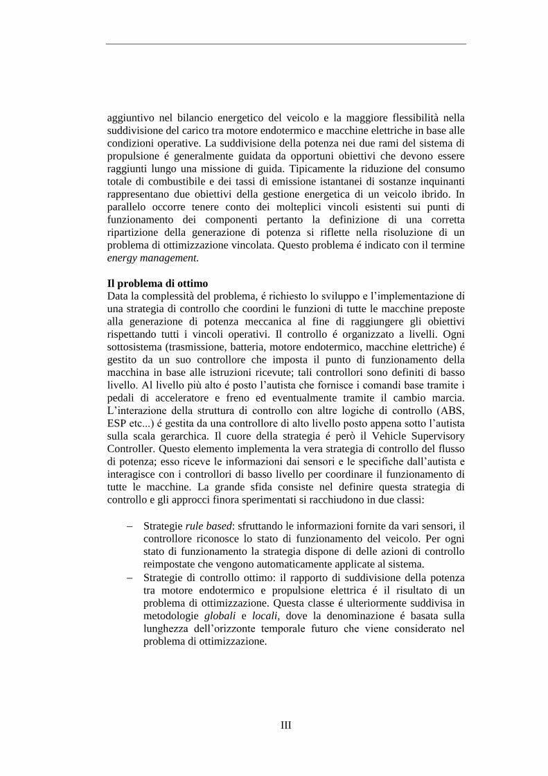
motore endotermico. Le prossime figure mostrano il progresso ottenuto in una
fase di avviamento.

Estratto in lingua italiana
XXII
Figura 9: Accelerazioni del corpo vettura
e velocità angolare dell'albero a gomiti.
Strategia euristica.
Figura 10: Accelerazioni del corpo vettura
e velocità angolare dell'albero a gomiti.
Strategia MPC.
La figura a sinistra mostra che la strategia rule based comanda repentinamente la
variazione della velocità angolare dell’albero a gomiti causando ampie
oscillazioni sia dell’accelerazione longitudinale che verticale del corpo vettura.
Lo stesso evento di avviamento comandato da MPC é rappresentato nelle figure
a destra. La curva seguita dalla velocità angolare é molto più dolce e l’effetto
sulle accelerazioni del corpo vettura é limitato. Questo comportamento é
raggiunto grazie ad un utilizzo completamente diverso della coppia del
generatore elettrico come mostrato nelle prossime due figure.
Figura 11: Utilizzo della coppia del
generatore elettrico durante l'avviamento
del motore endotermico. Strategia
euristica.
Figura 12: Utilizzo della coppia del
generatore elettrico durante l'avviamento
del motore endotermico. Strategia MPC.
Nel primo caso il picco della coppia é ben visibile e supera i 150 Nm, il periodo
di attivazione é limitato a 0.1 s. Nel secondo caso, il massimo valore di coppia é
inferiore a 7 Nm e poi MPC abbassa gradualmente il livello per raggiungere la
velocità di rotazione di minimo dopo circa 1s. il tempo totale di attivazione é
dunque molto più lungo ma se si osserva con attenzione le figure 9, 10 si nota

XXIII
come in entrambi i casi le funzioni del motore endotermico comincino a circa
58.5 s dunque MPC comincia la fase di avviamento prima rispetto alla rule
based per poi attivare la coppia allo stesso istante di tempo. Anche la strategia
rule based é in grado di raggiungere la medesima crescita dolce della variabile
modificando il guadagno proporzionale del controllore di basso livello che
comanda la coppia del generatore; dunque, trovando una soluzione al di fuori
della strategia stessa.
Seguendo le indicazioni riportate nella norma ISO 2631-5 e prendendo come
riferimento le fasi di Start&Stop del ciclo NEDC, é stata calcolata
l’accelerazione equivalente pesata a partire dalla accelerazione longitudinale,
verticale e di beccheggio del corpo vettura ed applicando le funzioni di peso
specificate nella norma per le suddette direzioni di misura. Per convenzione la
norma specifica che l’accelerazione equivalente dovrebbe risultare inferiore a
per non generare una sensazione sgradevole a bordo vettura. Tutte le
accelerazioni calcolate sono risultate inferiori a tale livello di soglia.
Stabilità della strategia MPC
A causa dei vincoli operativi e del fatto che la strategia é linearizzata ad ogni
istante di campionamento, non é possibile applicare alcuna regole della teoria
del controllo per garantire la stabilità della strategia. A tal scopo si é provveduto
a testare la strategia rispetto a differenti condizioni operative variando alcuni
parametri del modello. Ancora una volta si sono confrontati i risultati con quelli
ottenuti dalla strategia rule based. Tramite l’approccio One-At-a-Time si sono
ripetute una serie di simulazioni variando di volta in volta il livello di un
parametro solo, utilizzando il ciclo NEDC come ciclo di riferimento. I parametri
presi in esame sono stati la massa del corpo vettura, la pendenza della strada, il
coefficiente adimensionale di resistenza aerodinamica, la rigidezza della cinghia
di trasmissione, l’inerzia rotazionale delle ruote e il coefficiente di adesione
pneumatico - superficie stradale. Soltanto per i primi tre parametri si é osservato
una influenza sul consumo totale pertanto si riportano di seguito i risultati
relativi alle corrispondenti simulazioni.
Estratto in lingua italiana
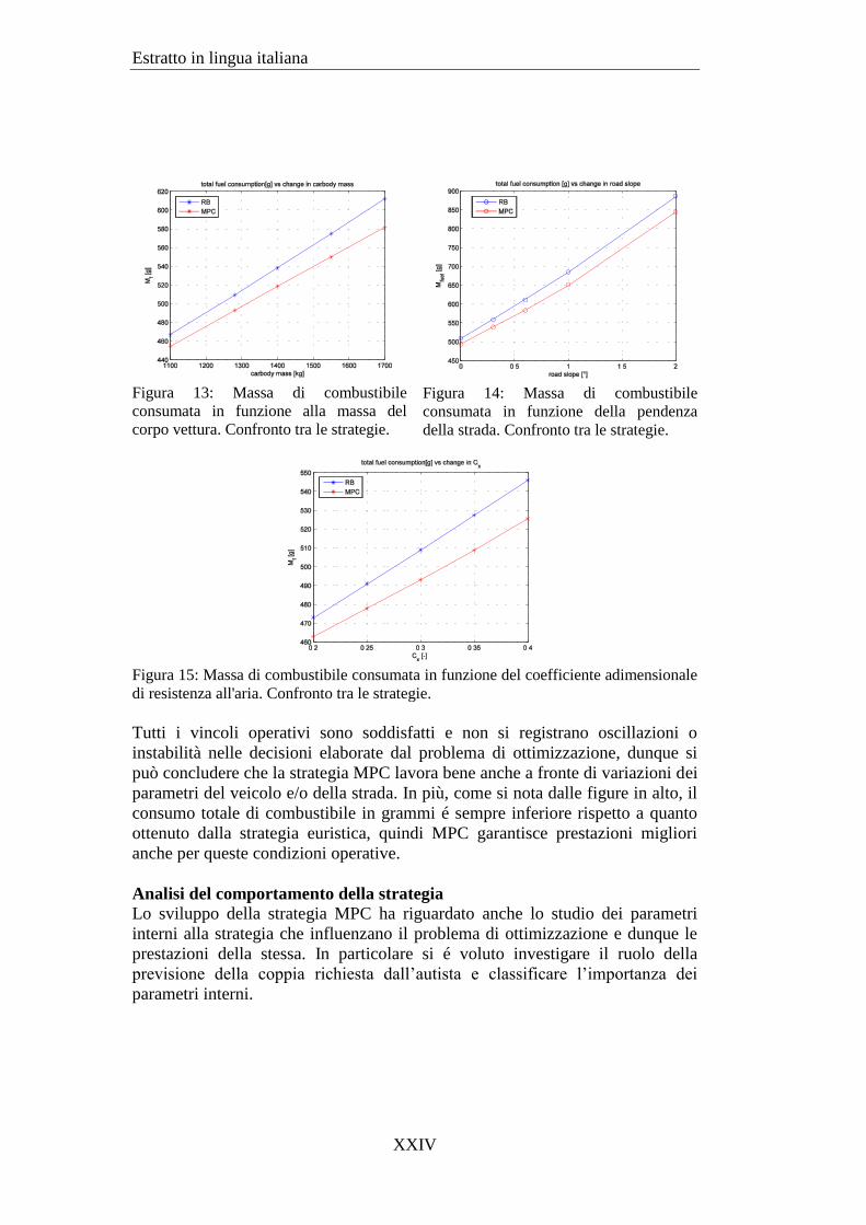
XXIV
Figura 13: Massa di combustibile
consumata in funzione alla massa del
corpo vettura. Confronto tra le strategie.
Figura 14: Massa di combustibile
consumata in funzione della pendenza
della strada. Confronto tra le strategie.
Figura 15: Massa di combustibile consumata in funzione del coefficiente adimensionale
di resistenza all'aria. Confronto tra le strategie.
Tutti i vincoli operativi sono soddisfatti e non si registrano oscillazioni o
instabilità nelle decisioni elaborate dal problema di ottimizzazione, dunque si
può concludere che la strategia MPC lavora bene anche a fronte di variazioni dei
parametri del veicolo e/o della strada. In più, come si nota dalle figure in alto, il
consumo totale di combustibile in grammi é sempre inferiore rispetto a quanto
ottenuto dalla strategia euristica, quindi MPC garantisce prestazioni migliori
anche per queste condizioni operative.
Analisi del comportamento della strategia
Lo sviluppo della strategia MPC ha riguardato anche lo studio dei parametri
interni alla strategia che influenzano il problema di ottimizzazione e dunque le
prestazioni della stessa. In particolare si é voluto investigare il ruolo della
previsione della coppia richiesta dall’autista e classificare l’importanza dei
parametri interni.

XXV
Previsione della coppia alle ruote
Il metodo MPC si basa sulla previsione degli accadimenti futuri per risolvere un
problema di ottimizzazione e calcolare le azioni di controllo da applicare al
sistema quindi é interessante capire l’influenza del modello adottato per
prevedere la coppia richiesta dall’autista alle ruote. Il modello previsionale
impiegato nello sviluppo della strategia descrive la coppia richiesta secondo un
decadimento esponenziale il cui valore iniziale coincide con il livello
campionato mentre il tasso di decadimento varia in relazione al livello di
potenza richiesto. In alternativa si é assunto che il veicolo disponga di sistemi di
navigazione quali GPS e GIS e che esso ripetesse assiduamente la stessa
missione di guida giorno per giorno. Questo é il caso ad esempio degli autobus
che seguono sempre lo stesso percorso. Con questa ipotesi é possibile assegnare
alla strategia MPC l’andamento preciso della potenza richiesta lungo l’orizzonte
di previsione. Infatti é lecito assumere che il profilo desiderato di velocità
corrisponda alla velocità media registrata su una serie di ripetizioni della
medesima missione di guida e allo stesso modo la coppia richiesta dall’autista e
ottenuta con precedenti simulazioni, rappresenti la coppia richiesta in media
dall’autista. Per semplificare l’analisi e per consentire alla strategia MPC di
lavorare nelle migliori condizioni operative possibili, sono stati forniti in
ingresso sia il profilo desiderato di velocità che un profilo di coppia ottenuto da
una simulazione test. In tal modo la previsione di queste due variabili lungo
l’orizzonte di previsione é pressoché esatta a meno di piccolissime e trascurabili
differenze nella coppia. Questa situazione é irrealistica ma lo scopo di questa
analisi é quello di investigare l’influenza della previsione della coppia, e
conseguentemente della velocità di avanzamento, sulle prestazioni della
strategia di controllo. I cicli NEDC e HWFET sono stati scelti come riferimento,
entrambi modificati per includere una variazione altimetrica lungo il percorso. I
risultati mostrati di seguito fanno riferimento alle simulazioni realizzate con la
strategia nominale e alle simulazioni realizzate con la strategia che riceve in
ingresso la descrizione esatta del profilo di coppia e di velocità.
Tabella 3: Confronto del consumo totale tra la strategia MPC nominale e la
strategia supportata da GPS/GIS.
Ciclo
Strategia
NEDC HWFET
Nominal 518.72 761.35
Exact prediction 518.50 761.0
Dai risultati emerge inaspettatamente un’influenza pressoché nulla della
previsione sulle prestazioni della strategia. La spiegazione a questa conclusione
si può trovare osservando, ad esempio, le sequenze dei valori ottimi della coppia
del motore a combustione interna lungo l’orizzonte di controllo ottenuti da

Estratto in lingua italiana
XXVI
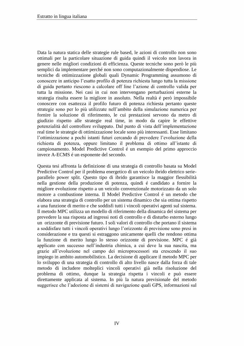
successivi problemi di ottimo. La prossima figura riporta alcune di queste
sequenze definite sul ciclo NEDC per un tratto di accelerazione.
Figura 16: Sequenze dei valori ottimi della coppia del motore endotermico calcolate
come soluzione di successivi problemi di ottimizzazione.
Queste sequenze sono state ottenute dalla strategia che riceve in ingresso gli
andamenti corretti delle variabili esterne misurate; si nota come MPC definisca
un andamento crescente della coppia nella primissima porzione dell’orizzonte di
controllo mentre nella seconda parte riduce velocemente la coppia. Ricordando
che lo scopo della strategia é quello di minimizzare la funzione di merito
quadratica lungo tutto l’orizzonte di previsione, questo andamento della
sequenza ottima si può spiegare con il tentativo da parte della strategia di ridurre
la deviazione dello stato di carica della batteria nella prima porzione
dell’orizzonte di previsione utilizzando la potenza del motore a combustione
interna, invece nella seconda porzione essa riduce la coppia erogata dal motore
endotermico per minimizzare il consumo totale su tale orizzonte. In quest’ottica
il problema di ottimizzazione sembra essere governato principalmente dal livello
di potenza richiesto e dall’entità della deviazione dello stato di carica della
batteria, all’istante di campionamento. Questa conclusione spiega il motivo per
cui modificando la previsione degli ingressi misurati non si registra un
cambiamento nei valori ottimi delle variabili di controllo determinati dalla
strategia.
Analisi di sensibilità dei parametri interni
La strategia di controllo MPC é caratterizzata da molti parametri interni quali ad
esempio la lunghezza dell’orizzonte di controllo, i pesi dei termini della
295 300 305 310 315 320 325 330
0
10
20
30
40
50
60
70
Optimal sequence of engine torque
t [s]
Te [
Nm
]

XXVII
funzione di merito, il tasso di decadimento esponenziale della previsione della
coppia richiesta alle ruote etc...
I valori di tutti questi parametri sono stati fissati mediante una lunga messa a
punto manuale basata sulla ripetizione di numerose simulazioni, pertanto é
interessante capire se esistono altri set di valori tali da garantire prestazioni
migliori della strategia i.e minor consumo di combustibile. Inoltre vale la pena
investigare la possibilità che, a seconda delle condizioni di guida e del veicolo, il
set ottimale dei valori dei parametri possa cambiare; in particolare in relazione
alla massa del veicolo può essere opportuno modificare il valore di uno o più
parametri per raggiungere una migliore efficienza energetica. Questa ultima
considerazione può rivelarsi utile negli autocarri dove é possibile avere una
stima della variazione della massa trasportata sfruttando le valvole sensibili alla
variazione di carico.
Per trovare una risposta a questi due punti é stata condotta una ampia analisi di
sensibilità su alcuni parametri interni della strategia con lo scopo di identificare
una superficie di risposta tra due uscite del sistema (i.e. consumo totale e livello
di equilibrio dello stato di carica) e alcuni parametri importanti della strategia.
Sfruttando l’esperienza maturata durante la procedura di messa a punto manuale,
5 parametri sono stati considerati più importanti: la lunghezza dell’orizzonte di
previsione, il numero di step nell’orizzonte di previsione per i quali i pesi della
funzione di merito sono modulati da un andamento a decadimento esponenziale,
la lunghezza dell’orizzonte di controllo, i pesi applicati sulla deviazione dello
stato di carica della batteria e sul consumo istantaneo di combustibile. Per questi
due ultimi parametri si é considerato la variazione rispetto al valore nominale. I
cicli NEDC e HWFET sono stati scelti come riferimento, due valori della massa
del corpo vettura sono stati considerati, in questo modo l’analisi ha sperimentato
diverse condizioni di guida per trarre il maggior numero di informazioni. Inoltre
le analisi hanno testato un ampio campo del dominio di ogni parametro al fine di
catturare eventuali dipendenze non lineari tra le uscite del sistema e i parametri.
Le tecniche consolidate della Design Of Experiment sono state ampiamente
impiegate, partendo con un’analisi su due livelli a fattoriale completo dei cinque
parametri e proseguendo con la determinazione si superfici di risposta delle due
uscite basate su campionamento Central Composite Design. Le superfici di
risposta sono stati ottenute per soli 4 parametri siccome l’analisi a fattoriale
completo ha mostrato la ridotta influenza della lunghezza dell’orizzonte di
controllo.
Le conclusioni che si possono trarre sono innanzitutto una generale insensibilità
delle uscite del sistema dal particolare ciclo di guida considerato oppure dalla
massa del veicolo. In questo senso la strategia MPC non é legata a particolari
condizioni di guida ma il suo comportamento si ripete inalterato per diversi cicli

Estratto in lingua italiana
XXVIII
di guida. Importante é osservare che variando il livello dei parametri interni
rispetto alla condizione nominale definita nella messa a punto manuale si
producono larghe variazioni del livello di equilibrio dello stato di carica della
batteria, i.e. fino a livelli. Al contrario la massa totale di combustibile non
mostra la stessa dipendenza, si registrano variazioni contenute nell’ordine dei
pochissimi grammi o frazioni del grammo anche per ampi intervalli dei livelli
dei parametri interni. In particolare l’utilizzo delle superfici di risposta consente
di concludere che il set ottimale dei parametri interni che minimizza il consumo
totale é molto vicino al set definito mediante la messa a punto manuale. I
parametri interni che hanno la maggiore influenza sul livello di equilibrio dello
stato di carica della batteria sono la lunghezza dell’orizzonte di previsione e il
peso della deviazione dello stato di carica della batteria.
Conclusioni
La strategia di controllo basata su MPC ha dimostrato di raggiungere un
consumo totale inferiore rispetto a una strategia euristica quando testate su cicli
di guida standardizzati. Sul ciclo di guida urbano UDDS la riduzione
percentuale di consumo é pari a -0.84 %, sul ciclo di guida autostradale HWFET
la riduzione percentuale é pari a -1.28 %. I cicli NEDC, SC03 e US06
coinvolgono condizioni di guida miste urbane ed extraurbane e soprattutto
richiedono un maggior sforzo da parte del sistema di propulsione. In questi casi
la strategia MPC ottiene i risultati migliori grazie alla profonda sinergia tra
motore endotermico e batteria; la riduzione percentuale di consumo totale é pari
a -3.12 %, -8.83 %, -17.75 % rispettivamente. Rispetto alla strategia euristica,
la strategia MPC é stata sviluppata per essere potenzialmente implementabile in
un controllore real time in quanto lavora a tempo discreto, ricorre a semplici
modelli di regressione polinomiale. La strategia si é dimostrata stabile rispetto
alla variabilità dei parametri del veicolo e/o della strada e la messa a punto dei
suoi parametri interni non é in alcun modo legata a un ciclo di guida specifico,
da questo punto di vista la strategia é più robusta rispetto, ad esempio, a A-
ECMS. La strategia si é dimostrata molto potente sapendo anche controllare le
fasi di avviamento e spegnimento del motore a combustione interna al fine di
limitare le vibrazioni conseguenti agenti sui passeggeri attraverso il corpo
vettura. L’accelerazione equivalente calcolata secondo le equazioni fornite dalla
norma ISO 2631-5, é risultata sempre essere inferiore al valore soglia
che indica una percezione sgradevole di una oscillazione ripetuta nel tempo.
Tuttavia emerge il problema di ricorrere ad una forma di stato linearizzata per
prevedere la risposta del sistema che introduce incertezza nella soluzione ottima
definita dal controllore. Le simulazioni al calcolatore hanno dimostrato che il
problema di ottimizzazione é risolvibile con successo entro il periodo di
campionamento di 0.1 s anche se rimane ancora da definire come dovrebbe
comportarsi la strategia in tutte quelle situazioni in cui il problema risolta essere

XXIX
mal posto, non risolvibile. Questo problema é ad ogni modo comune a tutte le
strategie di controllo basate sulla risoluzione di una funzione di merito. Non di
meno il problema di ottimo sembra essere governato principalmente dal valore
di deviazione dello stato di carica della batteria e dalla potenza richiesta
dall’autista, all’istante di campionamento rendendo la strategia piuttosto statica
e non potendo sfruttare le informazioni aggiuntive fornite dai sistemi di
navigazione. Eventualmente questi dati potrebbero essere impiegati a un livello
di controllo superiore sulla scala gerarchica rispetto alla strategia MPC che in
base alle informazioni acquisite possa modificare alcuni parametri, ad esempio il
livello di riferimento dello stato di carica della batteria, escludere uno dei
termini della funzione di costo. Un’altra limitazione é rappresentata dal fatto che
MPC é un metodo model based quindi é necessario sviluppare un modello
semplice ma affidabile del sistema di propulsione del veicolo e ogni modifica
apportata a questo assieme implica la definizione di un modello nuovo con
conseguente validazione.

Estratto in lingua italiana
XXX

XXXI


i
Table of contents
1 Introduction .................................................................................................... 1
2 Alternative propulsion systems ...................................................................... 3
2.1 The importance of hybridization ............................................................ 3
2.2 Hybrid electric vehicles .......................................................................... 6
2.3 Control structure for energy management .............................................. 7
2.3.1 The hardware ................................................................................... 7
2.3.2 The formulation as a problem of optimum ..................................... 8
2.3.3 The algorithms - State of the art .................................................... 10
2.4 Drivability metrics ................................................................................ 15
3 Architectures of hybrid electric vehicles ..................................................... 17
3.1 Classification of hybrid electric vehicles ............................................. 17
3.1.1 Series hybrid electric vehicle ........................................................ 19
3.1.2 Parallel hybrid electric vehicle ...................................................... 20
3.1.3 Series/parallel hybrid electric vehicles .......................................... 21
3.1.4 Plug-In hybrid electric vehicles .................................................... 23
3.2 Driving modes of a power-split hybrid electric vehicle ....................... 23
3.3 Main components of the analyzed HEV ............................................... 27
3.3.1 Power-split drive ........................................................................... 27
3.3.2 Internal combustion engine ........................................................... 30
3.3.3 Electric machines .......................................................................... 31
3.3.4 High voltage battery ...................................................................... 32
3.3.5 The vehicle assembly .................................................................... 34
4 The MPC-based control strategy ................................................................. 37
4.1 Background........................................................................................... 37
4.2 Formulation of the MPC strategy ......................................................... 40
4.2.1 The reference simplified model .................................................... 40
4.2.2 The operating constraints .............................................................. 56
4.2.3 The cost function ........................................................................... 61
4.2.4 The linearized state space form ..................................................... 62

ii
4.2.5 Quadratic Programming and Active set method ........................... 65
4.3 How the strategy works ....................................................................... 66
5 Results ......................................................................................................... 71
5.1 Validation of the models ...................................................................... 71
5.2 Fuel economy ....................................................................................... 74
5.2.1 Drive cycles and charge sustenance ............................................. 74
5.2.2 Comparison of the results ............................................................. 75
5.2.3 The operating principles of the two control strategies.................. 78
5.2.4 A problem related to linearization ................................................ 86
5.3 Drivability ............................................................................................ 88
5.3.1 Velocity tracking error .................................................................. 88
5.3.2 Passengers discomfort related to engine starting and stopping .... 88
6 Additional analyses ..................................................................................... 97
6.1 Robustness of the control strategy ....................................................... 97
6.1.1 Carbody mass................................................................................ 98
6.1.2 Road slope .................................................................................. 101
6.1.3 Dimensionless coefficient of aerodynamic drag......................... 103
6.1.4 Parameters with low influence.................................................... 105
6.2 Analysis of internal parameters ......................................................... 107
6.2.1 Sensitivity analysis ..................................................................... 107
6.2.2 Integration of GPS/GIS............................................................... 122
7 Conclusions and future works ................................................................... 127
Appendix A - Matrix approach to MPC ........................................................... 131
Appendix B - Sensitivity analysis and RSM .................................................... 139
Appendix C - Standard drive cycles ................................................................. 147
Bibliography ..................................................................................................... 151

iii
List of figures
Figure 2.1: Mitshubishi i-Miev [4]....................................................................... 4 Figure 2.2: Tesla Roadster [4] .............................................................................. 4 Figure 2.3: Control structure for the energy management of a hybrid electric
vehicle ................................................................................................................... 7 Figure 2.4: The eight working states of the rule based strategy [6] ................... 11
Figure 3.1: Layout of the powertrain of a series HEV ....................................... 19 Figure 3.2: Layout of the powertrain of a parallel HEV .................................... 21 Figure 3.3: Components of a power-split hybrid electric vehicle ...................... 22
Figure 3.4: Components of a 2x2 series/parallel HEV ...................................... 22 Figure 3.5: 3D view of the powertrain of a power-split HEV [19] .................... 23 Figure 3.6: Power flow in electric mode [19] .................................................... 24 Figure 3.7: Positive split mode. C and B mark two paths for engine power to the
wheels [19]. ......................................................................................................... 26 Figure 3.8: Positive split mode. the engine power is used to charge the battery
[19]. ..................................................................................................................... 26 Figure 3.9: Regenerative braking. Part of vehicle’s kinetic energy is recovered
in the high voltage battery [19]. .......................................................................... 27 Figure 3.10: Planar view of the transaxle. The engine is connected to the carrier,
the generator to the sun while the ring gear and the motor deliver the traction
torque to propel the vehicle [19]. ........................................................................ 28 Figure 3.11: Simplified model of a planetary gear set type I ............................. 28
Figure 3.12: Fuel mass flow rate [g/s] as function of engine torque and speed.
The engine OOL is the green curve. ................................................................... 30
Figure 3.13: Characteristic curves of the engine. Maximum, minimum torque
and engine OOL. ................................................................................................. 30
Figure 3.14: Output torque as function of input voltage and rotor angular
velocity. ............................................................................................................... 32
Figure 3.15: Power losses as function of output torque, rotor angular velocity
[19]. ..................................................................................................................... 32 Figure 3.16: Arrangement of battery banks. Equivalent electric circuit of a
single battery cell [19]. ........................................................................................ 33 Figure 3.17: Internal resistance of a cell as function of state of discharge and
temperature. ......................................................................................................... 33 Figure 3.18: Open circuit voltage of a cell as function of state of discharge and
temperature. ......................................................................................................... 33 Figure 4.1: (a). (left) A system may move from Xo to XN following three
possible different trajectories. (b) (middle) the constraints are dynamic and the
optimal trajectory needs to be recomputed. (c) (right) MPC updates the optimal
control action at each sampling time. .................................................................. 38

iv
Figure 4.2: Equivalent electric circuit which models the battery ...................... 43 Figure 4.3: Simplified scheme of the mechanical side of the powertrain ......... 45 Figure 4.4: Original (blue) and new (red) grid of values of engine torque and
speed. .................................................................................................................. 49
Figure 4.5: 11 Experimental curves which represent fuel mass flow rate as
function of engine speed and engine torque. ...................................................... 50 Figure 4.6: An example of interpolation of fuel consumption over the new set of
engine torque values for curve number 8. .......................................................... 50
Figure 4.7: Extrapolation to calculate the new value of fuel consumption for a
null value of engine torque. ................................................................................ 51
Figure 4.8: The new values of are connected to one another by a surface for
a better visualization and the surface is superimposed to the original curves. ... 51 Figure 4.9: Polynomial regression model of fuel flow rate over the entire
operating domain of the engine. ......................................................................... 52 Figure 4.10: Regression surface of power loss in the electric machines. .......... 53
Figure 4.11: Rgression surface of power loss in the electric machines. Second
view..................................................................................................................... 53 Figure 4.12: Experimental values of power loss (blue circles) and regression
model (red curve). Discrepancies between the experimental values and the
estimated values using the regression model. ..................................................... 54 Figure 4.13: Cell internal resistance. Experimental data (blue circles) and
correspondent data obtained from the regression model (red circles). ............... 55 Figure 4.14: Characteristic curves of the engine and correspondent
simplification with lines. .................................................................................... 57 Figure 4.15: Characteristic curve of the electric machines................................ 59 Figure 4.16: Complete operating domain of the electric machines. ................... 59
Figure 4.17: Example of linearization of the characteristic curve of the electric
machines. ............................................................................................................ 59
Figure 5.1: Battery SOC as obtained with Amesim® and the nonlinear model. . 72
Figure 5.2: Crankshaft angular velocity as obtained with Amesim® and the
nonlinear model. ................................................................................................. 72
Figure 5.3: Comparison of power loss in the motor. ......................................... 72 Figure 5.4: Comparison of fuel mass flow rate. ................................................ 72 Figure 5.5: Power loss in the generator. Comparison between Amesim
® and the
linearized SS form. ............................................................................................. 73 Figure 5.6: Percentage reduction of fuel consumption given by MPC with
respect to the rule based strategy. ....................................................................... 75 Figure 5.7: Comparison of battery state of charge level over the 5 considered
drive cycles as obtained with the rule based strategy (blue curves) and the MPC-
based strategy (red curves). a) top left NEDC, b) top right HWFET, c) mid left
SC03, d) mid right UDDS, e) low US06 ............................................................ 77 Figure 5.8: Velocity profile of the driving situation used to analyze the
operating principle of the MPC strategy. ............................................................ 78
v
Figure 5.9: Correspondent power flow in the powertrain. ................................. 79 Figure 5.10: Battery state of charge and engine torque for two repetitions of the
same velocity profile. .......................................................................................... 80 Figure 5.11: Velocity profile which corresponds to the considered driving
situation. .............................................................................................................. 81 Figure 5.12: Power flow in the powertrain as obtained with the rule based
strategy (left)and with MPC (right)..................................................................... 81 Figure 5.13: Engine operating points as obtained with the rule based strategy
(left) and with MPC (right). ................................................................................ 82 Figure 5.14: Velocity profile of the considered portion of HWFET.................. 83 Figure 5.15: Power flow with the rule based strategy in HWFET. .................... 83
Figure 5.16: Power flow with MPC in HWFET. ................................................ 83 Figure 5.17: Engine operating points defined by the rule based strategy. ......... 84 Figure 5.18: Engine operating points obtained with MPC. ................................ 84 Figure 5.19: Engine efficiency over the analyzed driving situation. ................. 85
Figure 5.20: Generator angular velocity during parallel driving mode in
HWFET. .............................................................................................................. 86
Figure 5.21: Generator angular velocity once its reference value is included in
the cost function. ................................................................................................. 87
Figure 5.22: Power flow in the powertrain once the reference value of generator
angular velocity is introduced. ............................................................................ 87
Figure 5.23: Carbody accelerations during engine starting. .............................. 89 Figure 5.24: Carbody jerks during engine starting............................................. 89 Figure 5.25: Carbody accelerations with a lower proportional gain. ................. 90
Figure 5.26: Carbody jerks with a lower proportional gain. .............................. 90 Figure 5.27: Generator torque for a unitary proportional gain. .......................... 90
Figure 5.28: Generator torque for a proportional gain equal to 0.1. ................. 90 Figure 5.29: Carbody accelerations due to engine starting obtained with MPC.
............................................................................................................................. 93
Figure 5.30: Generator torque defined by MPC to start the engine. .................. 94 Figure 5.31:Longitudinal acceleration ................................................................ 94
Figure 5.32: Vertical acceleration. ...................................................................... 94 Figure 5.33: Pitch acceleration. ........................................................................... 94 Figure 5.34: Carbody accelerations during engine stopping. ............................. 96
Figure 6.1: Battery SOC equilibrium level as function of carbody mass change.
............................................................................................................................. 99
Figure 6.2: Total fuel consumption as function of carbody mass change. ......... 99 Figure 6.3: Engine power as function of carbody mass levels. ........................ 100 Figure 6.4: Engine torque as function of carbody mass. .................................. 101 Figure 6.5: Engine speed as function of carbody mass. ................................... 101 Figure 6.6: Road height as function of vehicle absolute position. Road slope is
equal to 0.6° and the absolute position of carbody center of gravity is 3422.85
m. ....................................................................................................................... 102

vi
Figure 6.7: SOC equilibrium level as function of road slope. ......................... 102 Figure 6.8: Fuel consumption as function of road slope. ................................. 102 Figure 6.9: Time history of the SOC level as function of road slope. ............. 103 Figure 6.10: SOC equilibrium level as function of Cx .................................... 104
Figure 6.11: Fuel consumption as function of Cx. .......................................... 104 Figure 6.12: SOC equilibrium level correspondent to the 11 configurations
listed above. ...................................................................................................... 106 Figure 6.13: Total fuel consumption correspondent to the 11 configurations
listed above. ...................................................................................................... 106 Figure 6.14: Coefficients of influence on SOC. NEDC 1280kg. .................... 113 Figure 6.15: Coefficients of influence on fuel consumption. NEDC 1280kg . 113
Figure 6.16: Coefficients of influence on SOC. NEDC 1650kg. .................... 114 Figure 6.17: Coefficients of influence on fuel consumption. NEDC 1650kg. 114 Figure 6.18: Coefficients of influence on SOC. HWFET 1280kg. ................. 114 Figure 6.19: Coefficients of influence on fuel consumption. HWFET 1280kg.
.......................................................................................................................... 114 Figure 6.20: 25 values of SOC final level. NEDC 1650kg. ............................ 116
Figure 6.21: 25 values of fuel consumption. NEDC 1650kg. ......................... 116 Figure 6.22: 25 values of SOC final level. HWFET 1650kg Conf. B. ............ 116
Figure 6.23: 25 values of fuel consumption.HWFET 1650kg Conf B. ............ 116 Figure 6.24: Normal probability plot of the residuals. .................................... 118
Figure 6.25: Total fuel consumption for low, base and high level of Hp. ....... 119 Figure 6.26: Total fuel consumption as function of Hp. HWFET. .................. 120 Figure 6.27: Total fuel consumption as function of Hp. NEDC. ..................... 120
Figure 6.28: Road slope and velocity profile for NEDC. ................................ 123 Figure 6.29: Road slope and velocity profile for HWFET. ............................. 123
Figure 6.30: Sequence of optimal values of engine torque. HWFET. ............. 124 Figure B.1: Full factorial design ...................................................................... 141 Figure B.2: CCD-design. ................................................................................. 141
Figure B.3: The test configurations taken by three different design matrices. 144 Figure C.1: Reference velocity profile of cycle NEDC ................................... 147
Figure C.2: Reference velocity profile of cycle HWFET ................................ 147 Figure C.3: Reference velocity profile of cycle SC03 ..................................... 148 Figure C.4: Reference velocity profile of cycle UDDS ................................... 148
Figure C.5: Reference velocity profile of cycle US06 .................................... 149
vii
List of tables
Table 2.1: Technical data of two electric vehicles ................................................ 5
Table 4.1: Regression coefficients of the polynomial regression model for fuel
flow rate. ............................................................................................................. 53 Table 4.2: Coefficients used to define the linear constraints of the engine
characteristic curves. ........................................................................................... 58
Table 4.3: Coefficients used to define the linear constraints of the electric
machines on maximum torque. ........................................................................... 60 Table 4.4: Penalty weights defined in the cost function. .................................... 68 Table 5.1: Comparison of fuel economy. Final results. ...................................... 75
Table 5.2: Fuel economy and battery state of charge equilibrium level over the
urban portion of NEDC. ...................................................................................... 82 Table 5.3: Velocity tracking error. Mean value and standard deviation. ............ 88
Table 5.4: Equivalent accelerations related to engine start&stop events. ........... 96 Table 6.1: Performance of the two strategies against carbody mass variation. .. 99 Table 6.2: Fuel economy percentage variation with respect to carbody mass. . 100
Table 6.3: Values of the results displayed in the two figures above. ................ 102 Table 6.4: Fuel economy and percentage variation with respect to the base case.
........................................................................................................................... 103 Table 6.5: Values of SOC level and fuel consumption shown in the two figures
above. ................................................................................................................ 104 Table 6.6: Fuel economy and percentage variation with respect to the base case.
........................................................................................................................... 104 Table 6.7: SOC equilibrium level and total fuel consumption as function of
wheels rotary inertia. ......................................................................................... 105
Table 6.8: SOC equilibrium level and total fuel consumption as function of
silent chain stiffness. ......................................................................................... 105 Table 6.9: SOC equilibrium level and total fuel consumption as function of
adhesion coefficient tyre-road. .......................................................................... 105
Table 6.10: The 11 configurations that have been tested in this analysis. ........ 106
Table 6.11: Low and high levels of each factor. ............................................... 109 Table 6.12: Levels of each parameter taken for Configuration A..................... 110 Table 6.13: Levels of each parameter taken for Configuration B. .................... 111
Table 6.14: Design matrix of the DOE-CCD analysis. ..................................... 112 Table 6.15: Ci on SOC.NEDC 1280kg ............................................................. 113 Table 6.16: Ci on fuel. NEDC 1280kg. ............................................................. 113 Table 6.17: Ci on SOC. NEDC 1650kg. ........................................................... 114 Table 6.18: Ci on fuel. NEDC 1650kg. ............................................................. 114
Table 6.19: Ci on SOC. HWFET 1280kg. ........................................................ 114 Table 6.20: Ci on fuel. HWFET 1280kg. .......................................................... 114

viii
Table 6.21: Coefficients of the regression model of fuel consumption and SOC
minimum level. ................................................................................................. 117 Table 6.22: Comparison of the nominal against the optimal set of internal
parameters. ........................................................................................................ 120
Table 6.23: Fuel consumption with the nominal MPC strategy and the strategy
which knows perfectly the future power request. ............................................. 124 Table B.1: Design matrix of full factorial ........................................................ 142 Table B.2: Design matrix of CCD-design ........................................................ 142

ix
Nomenclature
: Cost function
: Battery state of charge [%]
: Simulation time [s]
: Fuel mass flow rate [g/s]
: Time [s]
: System states
: Control inputs
: External measured disturbances
: Fuel low heating value [J/kg]
: Electric power at battery’s terminals [W]
: Torque applied at the carrier [Nm]
: Torque applied at the ring gear [Nm]
: Torque applied at the sun gear [Nm]
: Angular velocity of the carrier [rad/s]
: Angular velocity of the ring gear [rad/s]
: Angular velocity of the sun gear [rad/s]
: Number of teeth of the sun gear [-]
: Number of teeth of the ring gear [-]
: Number of teeth of the carrier [-]
: Engine torque read from the look-up table [Nm]
: Set point of the engine torque [Nm]
: The engine friction torque at hot temperature read from a proper
table [Nm]
: The engine friction torque at cold temperature read from a proper
table [Nm]
: Engine torque obtained from a first order lag [Nm]
: Engine output torque at crankshaft [Nm]
: Air density [kg/m3]
: Reference air density value [kg/m
3]
: Engine time constant [s]
: Time constant of the electric machines [s]
: Set point of the electric machine torque read from a look-up table [Nm]
: Output torque produced at the rotor of the electric machines [Nm]
: Electric current through one cell of the battery [A]
: Electric voltage across one cell of the battery [V]
: Internal resistance of one cell of the battery [Ω]
: Open circuit voltage of one cell of the battery [V]
: Number of bans in parallel [-]

x
: Number of banks in series [-]
: Number of cells in series within each bank
: Voltage across a bank
: Battery electric current [A]
: Battery output voltage [V]
: Battery internal resistance [Ω]
: Battery open circuit voltage [V]
: Power released/absorbed by the battery [W]
: Charge of the battery [C]
: Battery rated capacity [As]
: Mass of the carbody plus mass of the engine [kg]
: Inertia of the front unsprung mass [kg]
: Inertia of the rear unsprung mass [kg]
: Total mass of the vehicle [kg]
: Combined rotary inertia of the two wheels of one axle [kgm
2]
: Static rolling radius of the wheel [m]
: Gear ratio introduced by the silent chain [-]
: Gear ratio of the final drive [-]
: Total gear ratio between the motor and the driven wheels [-]
: Rotary inertia of the rotor of the motor [kgm2]
: Rotary inertia of the flywheel [kgm2]
: Dimensionless coefficient of aerodynamic resistance [-]
: Vehicle front area [m2]
: Dimensionless coefficient of rolling resistance [-]
: Length of the prediction horizon [#samples]
: Length of the control horizon [#samples]
: Engine output torque at the crankshaft [Nm]
: Angular velocity of the crankshaft [rad/s]
: Motor output torque [Nm]
: Angular velocity of the rotor of the electric motor [rad/s]
: Generator output torque [Nm]
: Power released/absorbed by the electric motor [W]
: Power released/absorbed by the electric generator [W]
: Angular velocity of the rotor of the electric generator [rad/s]
: Driveline output torque [Nm]
: Angular velocity of the driven wheels [rad/s]
: Total braking torque applied by the service braking system [Nm]
: Total resistive force [N]
: Battery state of discharge [%]
: Total power loss in the electric machines [W]
: Power loss in the electric motor [W]

xi
: Power loss in the electric generator [W]
: Driving torque required by the driver at the sampling time [Nm]
: Total driving torque requested by the driver in the continuous time
domain [Nm]
: Power required by the driver at the sampling time [W]
: Fuel density [kg/m3]
: Equilibrium level of battery state of charge at the end of a cycle [%]
: Reference level of the battery state of charge [%]
: Reference value of the angular velocity of the rotor of the generator
[rad/s]
: Total fuel consumption [g]
: Linear stiffness of the silent chain [N/m]
: Dimensionless adhesion coefficient tyre-road [-]
: Penalty weight applied to the i-th term in the cost function [-]
: Weighted acceleration signal in the time domain [m/s2]
: Root means square of the acceleration signal in the time domain [m/s2]
: Crest factor of the acceleration signal [-]
: Sequence of system outputs over the prediction horizon
: Sequence of control inputs over the control horizon
: Sequence of external disturbances over the prediction horizon

xii
1 Introduction
Sustainable mobility is an impelling issue for the worldwide scientific
community and for the automotive industry. The reservoirs of hydrocarbons that
are currently exploited are expected to be consumed within few decades and it is
not guaranteed that new reservoirs will be found in the future. Furthermore
global warming is strongly affected by ground vehicles which are included
among the most important sources of pollutant gases in the atmosphere.
Automotive manufacturers are looking for new designs to produce
environmental-friendly vehicles and the research has been pointing towards
electrification of conventional powertrains to achieve highly efficient and less
polluting vehicles. This trend has brought to the introduction of full electric
vehicles, fuel cell electric vehicles and hybrid electric vehicles; however just for
the hybrid ones it is correct to talk of large production volume and they are the
most promising solution to the energy management problem now. The reason
for hybrid electric vehicles success over the other two types is that they match
the numerous objectives and constraints that driving a vehicle involves. The
most important objective is drivability, namely the powertrain should match the
driver’s power request in any driving situation provided that it is within its
operating boundaries.
For a hybrid vehicle traction power is produced by the electric machines and the
engine, therefore the additional targets is to produce power in the most efficient
way. The power split between electric machines and engine is constrained by the
characteristic curves of the machines, the necessity to guarantee a charge
sustaining hybrid and the necessity to limit the force transmissibility between
the powertrain and the passengers of the vehicle. As a consequence finding a
proper way to produce the traction power while satisfying all operating
constraints becomes a tough issue and it calls for an advanced strategy which
can set the correct power split for any driving situation.
In the past the control strategy was defined upon engineers’ experience on the
basis of pre-determined rules. Recently the theory of optimization has been
applied to the energy management problem and different approaches have been
used. Model Predictive Control is an approach to define a control action for a
dynamic system which is optimal in some sense; it has been recently applied to
the energy management problem since it can successfully handle multiple
constraints and objectives while attaining high performance. In literature it is
claimed that MPC can guarantee lower fuel consumption with respect to existing
approaches moreover due to its intrinsic predictive nature it may take advantage
of the cooperation with auxiliary navigation systems like GPS and GIS.

Chapter 1
2
As a result the aim of this thesis is to develop a MPC-based control strategy for
the energy management of a power-split hybrid electric vehicle in order to
assess its capability to deal with this problem. For this purpose the performance
of the strategy has been compared to those achievable with a rule based strategy
over some standard drive cycles. The high fidelity model of the whole
powertrain has been implemented in Amesim®
while the control strategy in
Simulink®
and the two software have been run in co-simulation. MPC is based
on a simplified linear model of the powertrain which allows the solver to
compute an optimal solution within a limited period of time. The linear matrix
approach allows the optimization problem to be expressed as a quadratic
programming problem where the property of convexity is guaranteed. An
improved Active-set algorithm has been used to solve the numeric optimization.
The results show that MPC manages to reduce total fuel consumption over all
standard drive cycles with respect to the rule based strategy. However the
strategy suffers from few weaknesses that should be taken into account in case
of real time implementation.
The thesis is organized in chapters; the next chapter, the second one of the
report, treats the energy management problem most while the third chapter
introduces the most typical hybrid powertrain architectures giving more insight
into the power-split architecture to highlight its strong sides and operating
modes. The fourth chapter introduces the MPC-based control strategy. The
theoretical background is briefly discussed while more insight is given into the
mathematical steps which enable to set up the optimization problem. The fifth
chapter shows the results in terms of fuel economy and drivability and compare
the rule based strategy to the MPC one. The sixth chapter cope with additional
analyses; in the first part a sensitivity analysis is used to catch the influence of
some factors on the performance of the strategy. In the second part a simple
implementation of additional input information coming from GPS and GIS is
presented. In the end some conclusions and comments are provided together
with an overview of possible future works.

3
2 Alternative propulsion systems
Ground transportation is accounted for one-third of the worldwide energy usage
[1] and fossil fuels still represent the primary energy source for ground vehicles
motion. The engine-powered vehicle is the most common architecture in
automotive industry due to its flexibility, compact design and ease of
transportation and storing of fuel. The energy necessary to drive a vehicle is
obtained from a combustion process which takes place in the combustion
chamber of an internal combustion engine. This process has two main important
drawbacks: the low efficiency and the pollutants which are generated as
products of the process. It is therefore not astonishing that the automotive
industry has been investing lots of resources on continuous refinement of engine
design and combustion process.
Specific targets in terms of fuel consumption and pollutant emission rates
reduction should be satisfied by any new vehicle that is put on the market.
Satisfying these constraints by improving solely the technology of engines and
combustion process is quite challenging, for this reason almost all automotive
manufacturers have already begun developing alternative propulsion systems
which can meet current and future environmental regulations. During the last
two decades electrification of automotive powertrain has been seen as a viable
solution to achieve better fuel economy and lower pollutant emissions. Three
main paths that have been followed by automotive manufactures and scientific
community:
Electric vehicles
Hybrid electric vehicles
Fuel cell hybrid electric vehicles
2.1 The importance of hybridization
The first solution is the most extreme one since it replaces the internal
combustion engine with an electric motor while the other two configurations
provides for using an internal combustion engine in collaboration with at least
one electric machine to achieve better overall efficiency and lower pollutant
emission rates. An internal combustion engine can provide maximum torque and
power within a limited speed range, in addition it can work efficiently only
within a limited domain of specific values of torque and angular velocity of the
crankshaft. Moreover an engine cannot deliver torque if the crankshaft is not
rotating meaning that it is necessary to install a clutch and a transmission in-
between the engine and the driven axle. On the other hand an electric motor for
traction application is characterized by a constant output torque, which
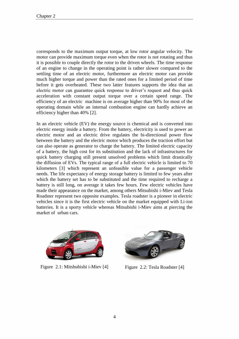
Chapter 2
4
corresponds to the maximum output torque, at low rotor angular velocity. The
motor can provide maximum torque even when the rotor is not rotating and thus
it is possible to couple directly the rotor to the driven wheels. The time response
of an engine to change in the operating point is rather slower compared to the
settling time of an electric motor, furthermore an electric motor can provide
much higher torque and power than the rated ones for a limited period of time
before it gets overheated. These two latter features supports the idea that an
electric motor can guarantee quick response to driver’s request and thus quick
acceleration with constant output torque over a certain speed range. The
efficiency of an electric machine is on average higher than 90% for most of the
operating domain while an internal combustion engine can hardly achieve an
efficiency higher than 40% [2].
In an electric vehicle (EV) the energy source is chemical and is converted into
electric energy inside a battery. From the battery, electricity is used to power an
electric motor and an electric drive regulates the bi-directional power flow
between the battery and the electric motor which produces the traction effort but
can also operate as generator to charge the battery. The limited electric capacity
of a battery, the high cost for its substitution and the lack of infrastructures for
quick battery charging still present unsolved problems which limit drastically
the diffusion of EVs. The typical range of a full electric vehicle is limited to 70
kilometers [3] which represent an unfeasible value for a passenger vehicle
needs. The life expectancy of energy storage battery is limited to few years after
which the battery set has to be substituted and the time required to recharge a
battery is still long, on average it takes few hours. Few electric vehicles have
made their appearance on the market, among others Mitsubishi i-Miev and Tesla
Roadster represent two opposite examples. Tesla roadster is a pioneer in electric
vehicles since it is the first electric vehicle on the market equipped with Li-ion
batteries. It is a sporty vehicle whereas Mitsubishi i-Miev aims at piercing the
market of urban cars.
Figure 2.1: Mitshubishi i-Miev [4]
Figure 2.2: Tesla Roadster [4]
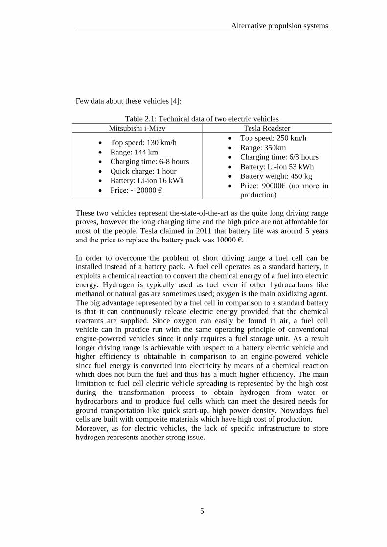
Alternative propulsion systems
5
Few data about these vehicles [4]:
Table 2.1: Technical data of two electric vehicles
Mitsubishi i-Miev Tesla Roadster
Top speed: 130 km/h
Range: 144 km
Charging time: 6-8 hours
Quick charge: 1 hour
Battery: Li-ion 16 kWh
Price: ~ 20000 €
Top speed: 250 km/h
Range: 350km
Charging time: 6/8 hours
Battery: Li-ion 53 kWh
Battery weight: 450 kg
Price: 90000€ (no more in
production)
These two vehicles represent the-state-of-the-art as the quite long driving range
proves, however the long charging time and the high price are not affordable for
most of the people. Tesla claimed in 2011 that battery life was around 5 years
and the price to replace the battery pack was 10000 €.
In order to overcome the problem of short driving range a fuel cell can be
installed instead of a battery pack. A fuel cell operates as a standard battery, it
exploits a chemical reaction to convert the chemical energy of a fuel into electric
energy. Hydrogen is typically used as fuel even if other hydrocarbons like
methanol or natural gas are sometimes used; oxygen is the main oxidizing agent.
The big advantage represented by a fuel cell in comparison to a standard battery
is that it can continuously release electric energy provided that the chemical
reactants are supplied. Since oxygen can easily be found in air, a fuel cell
vehicle can in practice run with the same operating principle of conventional
engine-powered vehicles since it only requires a fuel storage unit. As a result
longer driving range is achievable with respect to a battery electric vehicle and
higher efficiency is obtainable in comparison to an engine-powered vehicle
since fuel energy is converted into electricity by means of a chemical reaction
which does not burn the fuel and thus has a much higher efficiency. The main
limitation to fuel cell electric vehicle spreading is represented by the high cost
during the transformation process to obtain hydrogen from water or
hydrocarbons and to produce fuel cells which can meet the desired needs for
ground transportation like quick start-up, high power density. Nowadays fuel
cells are built with composite materials which have high cost of production.
Moreover, as for electric vehicles, the lack of specific infrastructure to store
hydrogen represents another strong issue.
Chapter 2
6
2.2 Hybrid electric vehicles
Hybrid electric vehicles represent instead a feasible response to current and
future problems related to everyday urban mobility and environmental issues.
The definition hybrid electric appeals to the architecture of the vehicle
powertrain which includes both a conventional powertrain based on an internal
combustion engine and an innovative powertrain based on electric and
mechanical components. The main reason to introduce additional components in
the powertrain is to support the internal combustion engine during all its
operations in order to shift its operating point to a region of high efficiency and
low emission rates.
It is straightforward to understand that by sharing the total power request
between the electric and the mechanical transmission paths a hybrid electric
vehicle can achieve better fuel economy than a conventional vehicle where the
engine has to balance the overall external load, however there is a number of
reasons which can justify the improvement of overall efficiency from tank-to-
wheel (1)
. Firstly, the main operating principle is load-leveling [1] meaning that
the total power request is split between the internal combustion engine and the
electric powertrain in such a way that the engine can always operate in a region
of high efficiency or at least close to it. The power split ratio is, for most of the
cases, not fixed but it can be varied depending on driving conditions. This
corresponds to a degree of freedom in the energy management of the vehicle
since the engine power can be either primarily sent to the driven wheels or used
to charge the battery. The battery power represents the second degree of
freedom. Suppose the engine worked always in its most efficient operating
point, during low power request it can provide more power than the required one
which is stored in the battery. During high power request the engine would not
generate the total traction effort because the battery would support it by
providing the necessary amount of power to match the total power request and
let the engine work in a region of high efficiency. The power split allows the
designer to install a downsized engine which can be optimized to work in a
specific speed range rather than assuring a good compromise between
performance and efficiency over the entire operating range.
Regenerative braking is applied in both electric and hybrid electric vehicles in
order to recover part of the mechanical energy of the vehicle during braking and
store it as electric energy into the battery; hence it is another possibility to
achieve better fuel economy since battery state of charge can be replenished
1 The overall efficiency of a vehicle should be evaluated considering the whole energy
transformation process which is organised n two steps: well-to-tank and tank-to-wheel. However
the current analysis considers only the latter.

Alternative propulsion systems
7
without using additional engine power. Lastly, full electric mode is available for
example during low speed driving and low power request, reverse motion; the
engine can be switched off during protracted stops if the battery is well charged.
The most important components of the powertrain are an internal combustion
engine that is flanked by at least one electric machine, an energy storage battery,
power electronics and a mechanical driveline. Hybrid vehicles can use the
already existing infrastructures for fuel replenishment and they can successfully
overcome typical limitations of EVs by using the internal combustion engine
power to charge the battery and run the vehicle. These improvements are
achieved at a price of higher complexity in the design and control of the
powertrain components and operations. In fact in order to exploit the benefits
that a hybrid architecture can guarantee in terms of fuel economy it is necessary
to blend the operations of all powertrain components so that they can cooperate
successfully. This requires the definition of a precise control strategy for energy
management which has to decide how the power flow should be split within the
powertrain, namely to what extent each machine should contribute to the
production of total power required. A similar control strategy is not needed in a
conventional engine powered vehicle since the internal combustion engine is the
unique power unit.
2.3 Control structure for energy management
2.3.1 The hardware
Due to the high complexity of the system and multiple input/output information
that have to be defined, the control is organized in a hierarchical structure which
is depicted in Figure 2.3.
Figure 2.3: Control structure for the energy management of a hybrid electric
vehicle

Chapter 2
8
The driver is at the top level of this structure. It is outside the system but it
defines the desired operating conditions of the powertrain in terms of torque and
power request. The driver behaves like a feedback controller since the driver
pushes either the throttle or the brake pedal depending on the error between the
actual vehicle velocity and the desired velocity which is in his mind. Moreover
sudden acceleration or braking commands can be provided depending on the
driving situations. A mode selector is placed in-between the driver and the
vehicle supervisory controller (VSC) [1] to change some internal parameters of
this latter depending on driving situations; for example if a sudden hard braking
is detected or a fault is detected in the system then the energy management
problem has no more the priority but vehicle safety and stability has to be
guaranteed. Therefore this additional controller takes over the control strategy
and drives the vehicle to a safe state. In addition it coordinates the operations of
the vehicle supervisory controller which considers only the energy management
problem with other active control systems that are implemented in the vehicle.
The lowest level comprises the control algorithms of all machines in the
powertrain. Each component in the powertrain has its dedicated control unit;
these units are regarded to as low-level controllers and some typical examples
are the engine controller, the gearbox controller, the electric machines
controller. These controllers have the task to regulate the behavior of a machine
in order to achieve a desired operating point. However these controllers have a
limited view and understanding of what is happening in the system; they are
only tuned to make a machine reach quickly the desired operating point while
satisfying operating constraints but they are not able to define the desired set
point on their own. For this reason a high level controller has the responsibility
to define the target operating point of each component of the powertrain; this
high level controller called vehicle supervisory controller has a global view of
the operations of the powertrain, the status of the vehicle and the requests from
the driver so it can properly define these desired operating points. The vehicle
supervisory controller is the module which translates the driver’s requests into
specific control signals for the powertrain. It communicates with both entities
and receives inputs from them. Throttle and brake pedal position are mapped to
obtain the desired torque request; for parallel hybrids an additional input from
the driver might be represented by the gear shifting command. Multiple signals
from sensors spread in the vehicle are used to analyze the vehicle status. All
inputs are processed and correspondent output control signals are provided to
low level controllers through the vehicle controller area network (CAN).
2.3.2 The formulation as a problem of optimum
The energy management problem is addressed directly in the VSC and it can be
idealized as a constrained optimization problem. It is designed in order to
achieve specific objectives like lower fuel consumption, lower pollutant

Alternative propulsion systems
9
emissions while satisfying at the same time a number of constraints which are
defined by the characteristics of the machines and drivability (i.e. how the
vehicle responds to driver’s requests). A typical constraint for a charge
sustaining hybrid is that the battery state of charge level has to remain within
two boundaries throughout the driving mission and the final level should be
close to the initial level. The objectives are usually defined by metrics or
mathematical functions: the definition depends on the objective itself; for
example fuel economy involves the minimization of the total fuel consumption
over the entire driving mission and the deviation of the battery state of charge at
the end of the mission with respect to a target value. An integral objective plus a
terminal cost on state of charge deviation summarize these targets:
(2.1)
Drivability may instead introduce objectives like attenuation of longitudinal jerk
during gear shifting or number of gear shifting. In this case the objective is to
minimize the total number of gear shifting events (GSE) within a driving
mission and the cost function may represent this total number .
(2.2)
In addition several constraints should be satisfied throughout the driving
mission. The constraint on sustenance of battery state of charge has already been
mentioned furthermore each component of the powertrain has a specific
operating domain which should be taken into account when power split is
defined otherwise desired setting points may not be achieved because they lie
outside this domain. Operating constraints are easily translated into
mathematical functions of system states and control inputs; depending on the
type of the problem external measured disturbances can also be considered.
Constraints can be represented via nonlinear functions as follows:
(2.3)
where is usually a vector of nonlinear functions.
Lastly, the energy management refers to a specific powertrain configuration
where control inputs, system states and external disturbances are connected to
one another. Different approaches are available to model a system; however a
state space form is the most useful one since it highlights the relationships
among system states, control inputs, external disturbances and system outputs.
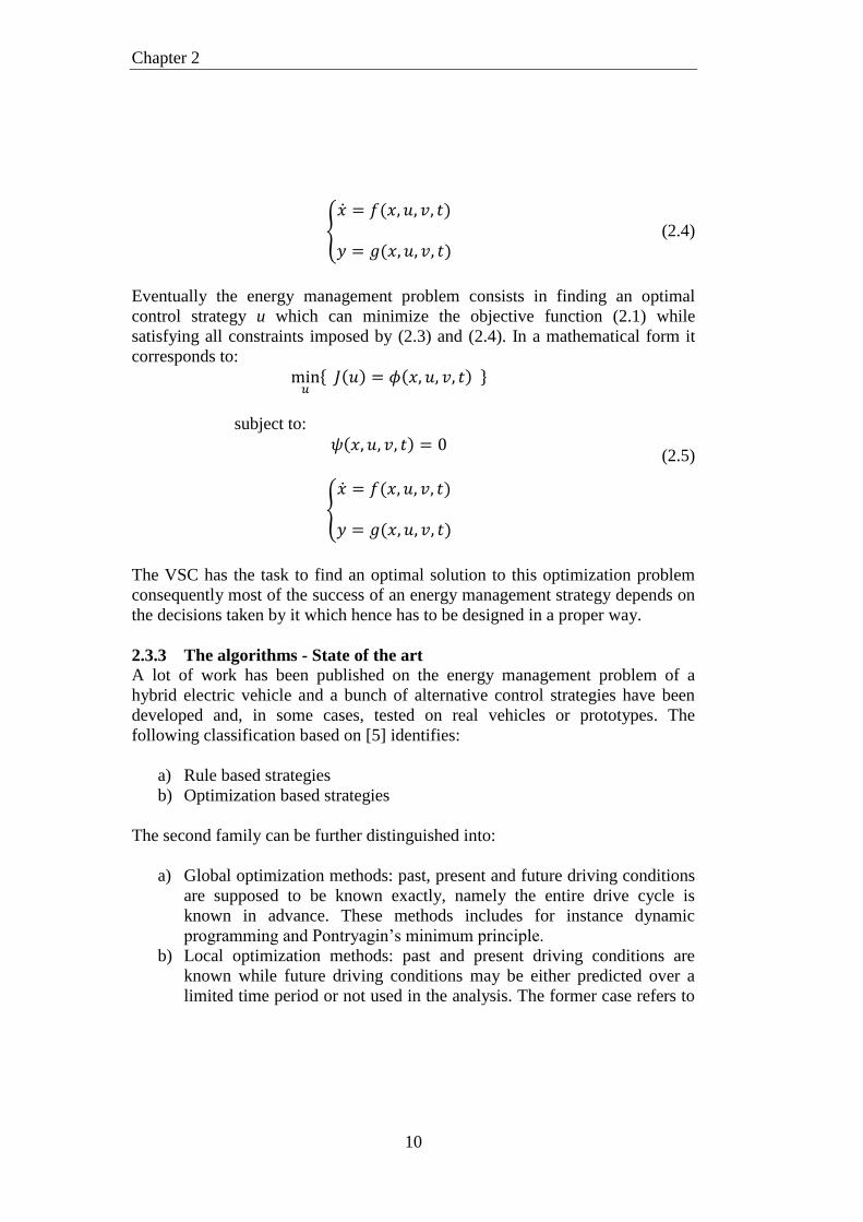
Chapter 2
10
(2.4)
Eventually the energy management problem consists in finding an optimal
control strategy u which can minimize the objective function (2.1) while
satisfying all constraints imposed by (2.3) and (2.4). In a mathematical form it
corresponds to:
subject to:
(2.5)
The VSC has the task to find an optimal solution to this optimization problem
consequently most of the success of an energy management strategy depends on
the decisions taken by it which hence has to be designed in a proper way.
2.3.3 The algorithms - State of the art
A lot of work has been published on the energy management problem of a
hybrid electric vehicle and a bunch of alternative control strategies have been
developed and, in some cases, tested on real vehicles or prototypes. The
following classification based on [5] identifies:
a) Rule based strategies
b) Optimization based strategies
The second family can be further distinguished into:
a) Global optimization methods: past, present and future driving conditions
are supposed to be known exactly, namely the entire drive cycle is
known in advance. These methods includes for instance dynamic
programming and Pontryagin’s minimum principle.
b) Local optimization methods: past and present driving conditions are
known while future driving conditions may be either predicted over a
limited time period or not used in the analysis. The former case refers to

Alternative propulsion systems
11
MPC and stochastic dynamic programming while the latter case refers to
ECMS.
Rule based strategies
A rule based strategy is also known as a heuristic control strategy since in most
of the cases it is defined upon engineers’ experience and personal judgment. The
control commands (desired operating points of the powertrain components) are
defined by a set of rules depending on the input information coming from driver
and vehicle sensors. These rules are similar to if-then [6]
programming
structures because the power split ratio between engine and battery is decided
depending on the required traction power and the battery state of charge level.
Once a driving condition is recognized, correspondent rules are triggered. As a
result these strategies do not try to find a numeric solution to the optimization
problem illustrated in (2.5), so it is not guaranteed that the resulting control
strategy is the optimal one moreover a tough tuning procedure of several
parameters is required to achieve decent fuel economy over different driving
scenario. Nonetheless due to their ease of implementation for real-time
application, heuristic rule based strategies are extensively applied to hybrid
electric vehicles available on the market today. In [6] a 8 states rule based
strategy is compared to other three control strategies. The scheme of the
heuristic control is reported in Figure 2.4.
Figure 2.4: The eight working states of the rule based strategy [6]
Alpha and beta represent respectively the normalized acceleration pedal position
and the normalized braking pedal position. The control output is the torque split
between engine and electric motor. As the scheme illustrates, the power split is
decided merely upon throttle and brake pedals position, torque request and
battery state of charge level.

Chapter 2
12
Dynamic programming
Dynamic programming is a method which calculates an optimal solution to (2.5)
which holds for the entire driving mission since it is assumed that power request
is completely know in advance. This corresponds to a huge limitation for real-
time applications because it is impossible to know in advance the whole effort
which is asked to the powertrain, nevertheless the optimal solution obtained
with dynamic programming can be used as benchmark for assessment of other
methods like for instance rule based. Dynamic programming has been widely
used in many papers where the known driving mission corresponds to one of the
standard drive cycles. If the system were not subjected to external disturbances
then the solution obtained with dynamic programming would be the optimal one
with the piece of advantage of being computed off-line. Unfortunately any real
system is subjected to external disturbances whose properties cannot be
completely known in advance; as a consequence if the optimal control strategy
were computed off-line using dynamic programming and then applied to the
system, it would produce poor performance and it may not guarantee the
stability of the system.
In order to overcome this problem either stochastic dynamic programming or
predictive dynamic programming [7] can be applied. Stochastic dynamic
programming predicts the future outcome of external disturbances according to
a Markov process. The stochastic properties of the probability distribution of
random external variables should be known in advance and this represents a
limitation for real-time application to the energy management problem. In fact
this requires knowing the stochastic properties of power request at wheels which
is very difficult when the driving mission is completely unknown. A partial
description of road, traffic conditions can be provided by navigation systems
however for the ease of real-time application the integration of all these tools
represents a stringent constraint. In [6] dynamic programming is used to set a
benchmark to assess the goodness of other three control strategies. In [8],
however, DP is used in combination to standard optimal control theory to
provide a control strategy for a parallel hybrid electric vehicle. On the other
hand a promising application of stochastic dynamic programming appeals to
those vehicles which are meant to repeat steadily the same route. In this case the
average power request can be described on the basis of collected measurements
of past repetitive driving missions. In [9] it is shown how stochastic dynamic
programming can be applied to the energy management problem of a bus for
public transportation whose mean power request profile can be determined in
advance by collecting data of several driving missions along the same route. In
[10], instead, Markov chains and Stochastic Dynamic Programming are even
applied to a series hybrid electric vehicle whose driving mission is unknown a
priori and power demand is obtained through a Markov process where stochastic
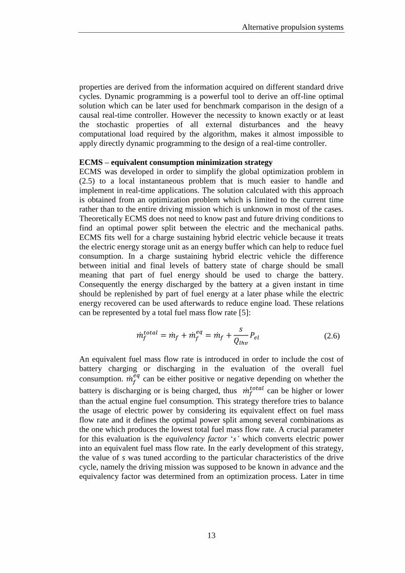
Alternative propulsion systems
13
properties are derived from the information acquired on different standard drive
cycles. Dynamic programming is a powerful tool to derive an off-line optimal
solution which can be later used for benchmark comparison in the design of a
causal real-time controller. However the necessity to known exactly or at least
the stochastic properties of all external disturbances and the heavy
computational load required by the algorithm, makes it almost impossible to
apply directly dynamic programming to the design of a real-time controller.
ECMS – equivalent consumption minimization strategy
ECMS was developed in order to simplify the global optimization problem in
(2.5) to a local instantaneous problem that is much easier to handle and
implement in real-time applications. The solution calculated with this approach
is obtained from an optimization problem which is limited to the current time
rather than to the entire driving mission which is unknown in most of the cases.
Theoretically ECMS does not need to know past and future driving conditions to
find an optimal power split between the electric and the mechanical paths.
ECMS fits well for a charge sustaining hybrid electric vehicle because it treats
the electric energy storage unit as an energy buffer which can help to reduce fuel
consumption. In a charge sustaining hybrid electric vehicle the difference
between initial and final levels of battery state of charge should be small
meaning that part of fuel energy should be used to charge the battery.
Consequently the energy discharged by the battery at a given instant in time
should be replenished by part of fuel energy at a later phase while the electric
energy recovered can be used afterwards to reduce engine load. These relations
can be represented by a total fuel mass flow rate [5]:
(2.6)
An equivalent fuel mass flow rate is introduced in order to include the cost of
battery charging or discharging in the evaluation of the overall fuel
consumption.
can be either positive or negative depending on whether the
battery is discharging or is being charged, thus can be higher or lower
than the actual engine fuel consumption. This strategy therefore tries to balance
the usage of electric power by considering its equivalent effect on fuel mass
flow rate and it defines the optimal power split among several combinations as
the one which produces the lowest total fuel mass flow rate. A crucial parameter
for this evaluation is the equivalency factor ‘s’ which converts electric power
into an equivalent fuel mass flow rate. In the early development of this strategy,
the value of s was tuned according to the particular characteristics of the drive
cycle, namely the driving mission was supposed to be known in advance and the
equivalency factor was determined from an optimization process. Later in time

Chapter 2
14
adaptive ECMS, or A-ECMS, was developed to deal with real applications
where driving mission is not known a priori. As example is provided in [11].
The equivalency factor is adapted to driving conditions and style by using recent
past information and possibly future information to detect the cycle type.
Another improvement considers route recognition where driving conditions are
acknowledged according to their mean characteristics and the equivalency factor
is updated from a table of stored values. A shifting time interval is considered
for route recognition so that the value of s can be updated frequently. Despite
the ECMS algorithm is much less computational demanding than dynamic
programming, still there are some issues related to its implementation. The
online route recognition and equivalency factor updating may require large
memory usage, moreover the optimal control inputs are found among a set of
discrete candidates similarly to DP. Therefore there is no assurance that the
optimal values are included in this group.
MPC – model predictive control
MPC was developed in chemical industry as preferred control strategy for slow
chemical processes. Model predictive control is undoubtedly a powerful tool to
control dynamic systems characterized by several constraints on systems states,
control inputs and outputs when a desired objective function should be
minimized. Nonetheless it solves continuously a numeric optimization problem,
hence its application in automotive industry is increasing besides the
improvement of computational capability of microcontrollers. In [12] it is used
to smoothen the transition between electric driving mode and hybrid mode
which causes torque fluctuations and undesired longitudinal accelerations in a
parallel hybrid electric vehicle. Many other examples of applications to
automotive industry are available in [13].
When applied to the energy management problem of a hybrid electric vehicle,
MPC can be seen as a step forward with respect to ECMS since it reduces the
global optimization problem in (2.5) to a local problem limited to a short future
time period where it uses predictions of future driving conditions to find an
optimal control action which can both satisfy all constraints and minimize the
objective function. In contrast with ECMS and DP, control inputs are not
discretized in values but they can assume any value inside the admissible
domain (although discretization is introduced by the computational capability of
the software). Applications of MPC to the energy management of a hybrid
vehicle is quite recent; among others, interesting examples of application to
series and power-split hybrids are [14], [15], [16]. In particular [14] gives some
insight into real-time application of MPC to this type of problem by highlighting
the strong limitations that exist.[15] shows the capability of MPC to deal with
multiple constraints while [16] assumes that torque equilibrium at the driveline
may not be satisfied at each instant and therefore vehicle velocity tracking is
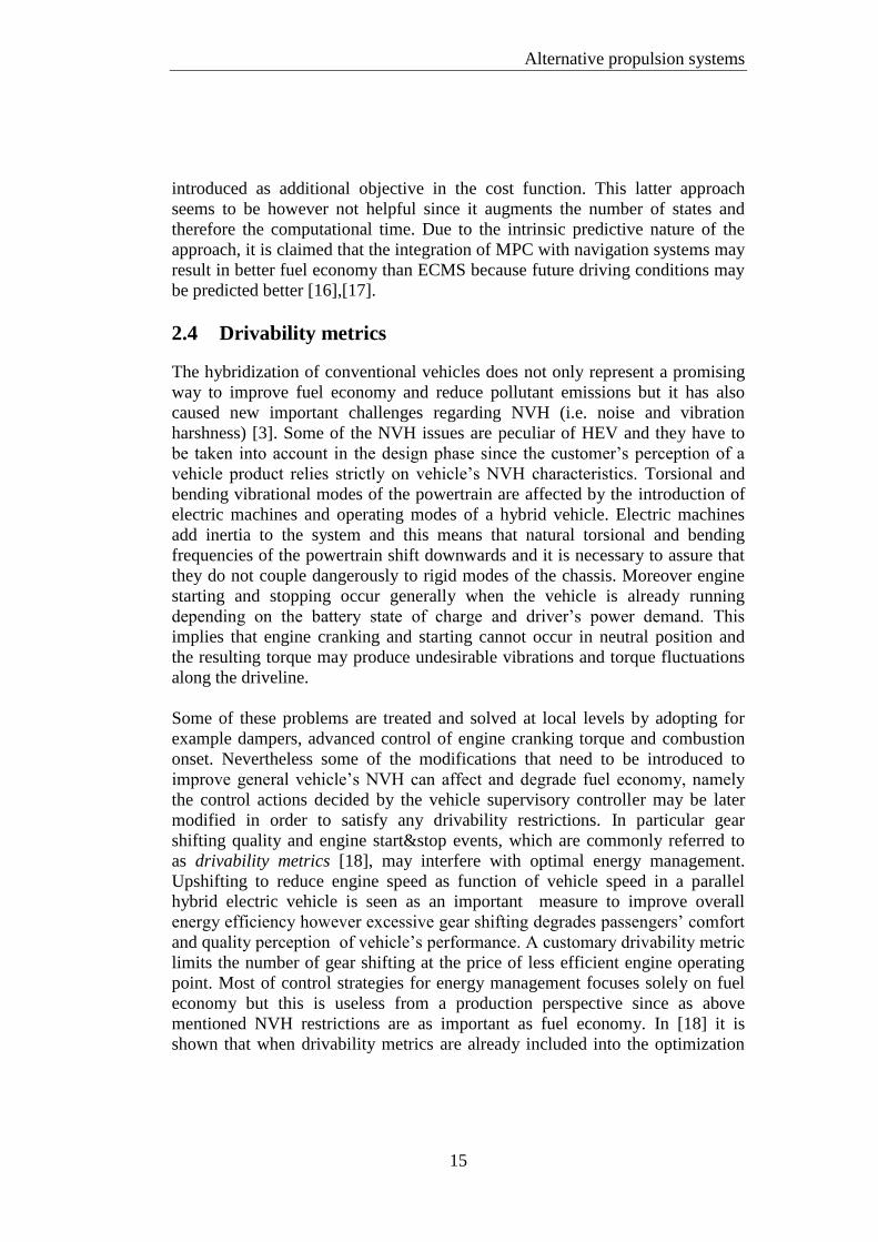
Alternative propulsion systems
15
introduced as additional objective in the cost function. This latter approach
seems to be however not helpful since it augments the number of states and
therefore the computational time. Due to the intrinsic predictive nature of the
approach, it is claimed that the integration of MPC with navigation systems may
result in better fuel economy than ECMS because future driving conditions may
be predicted better [16],[17].
2.4 Drivability metrics
The hybridization of conventional vehicles does not only represent a promising
way to improve fuel economy and reduce pollutant emissions but it has also
caused new important challenges regarding NVH (i.e. noise and vibration
harshness) [3]. Some of the NVH issues are peculiar of HEV and they have to
be taken into account in the design phase since the customer’s perception of a
vehicle product relies strictly on vehicle’s NVH characteristics. Torsional and
bending vibrational modes of the powertrain are affected by the introduction of
electric machines and operating modes of a hybrid vehicle. Electric machines
add inertia to the system and this means that natural torsional and bending
frequencies of the powertrain shift downwards and it is necessary to assure that
they do not couple dangerously to rigid modes of the chassis. Moreover engine
starting and stopping occur generally when the vehicle is already running
depending on the battery state of charge and driver’s power demand. This
implies that engine cranking and starting cannot occur in neutral position and
the resulting torque may produce undesirable vibrations and torque fluctuations
along the driveline.
Some of these problems are treated and solved at local levels by adopting for
example dampers, advanced control of engine cranking torque and combustion
onset. Nevertheless some of the modifications that need to be introduced to
improve general vehicle’s NVH can affect and degrade fuel economy, namely
the control actions decided by the vehicle supervisory controller may be later
modified in order to satisfy any drivability restrictions. In particular gear
shifting quality and engine start&stop events, which are commonly referred to
as drivability metrics [18], may interfere with optimal energy management.
Upshifting to reduce engine speed as function of vehicle speed in a parallel
hybrid electric vehicle is seen as an important measure to improve overall
energy efficiency however excessive gear shifting degrades passengers’ comfort
and quality perception of vehicle’s performance. A customary drivability metric
limits the number of gear shifting at the price of less efficient engine operating
point. Most of control strategies for energy management focuses solely on fuel
economy but this is useless from a production perspective since as above
mentioned NVH restrictions are as important as fuel economy. In [18] it is
shown that when drivability metrics are already included into the optimization

Chapter 2
16
problem (2.5), fuel consumption can be reduced by 10% in comparison to a
control strategy which has been only based on fuel economy aspects and later
modified to respect some NVH restrictions.
Due to the multiple constraints that characterize the energy management of a
hybrid electric vehicle and the appealing property of being predictive by nature
and suitable for implementation with auxiliary navigation systems, MPC has
been chosen to develop a control strategy for the vehicle supervisory controller.
3 Architectures of hybrid electric vehicles
There is a rather large nomenclature for hybrid electric vehicles depending on
the arrangement of the components in the powertrain and the rate of
hybridization of the propulsion system. In this chapter a short description of the
available classifications is provided then the different architectures of a hybrid
powertrain are introduced and briefly explained. In particular emphasis is put on
the comparison between series, parallel and series-parallel hybrid electric
vehicles with the aim to highlight advantages and disadvantages of each
configuration with respect to one another. Afterwards more insight on series-
parallel hybrid electric vehicles is provided since this architecture is analyzed
deeply in this thesis work. The driving operating modes are discussed and the
technical terminology, which is useful to understand some key concepts that
appear in the next chapters, is introduced and clarified. Lastly the layout of the
analyzed power-split hybrid electric vehicle is introduced and the main
components of the powertrain are characterized.
3.1 Classification of hybrid electric vehicles
A hybrid electric vehicle is equipped with an internal combustion engine and at
least one electric motor which contributes to generate the necessary traction
power. An electric energy storage unit provides electric power to the electric
motor and works as an energy buffer for the engine. Most of the time a battery
accomplishes this task however supercapacitors or fuel cell can also be used in
placed of a conventional battery. Moreover the battery technology can range
from lead acid to Li-ion batteries [1]. The powertrain that is discussed
afterwards implements a lead-acid battery. With respect to a conventional
passenger vehicle, the powertrain of a hybrid electric one can be seen as
composed by a mechanical and an electric path for power flow which are
connected to each other by mechanical and electric nodes. A planetary gear set
or another device for mechanical power transformation is a mechanical node
while power electronics represent an electric node. Blending of power between
these two paths is crucial to achieve high efficiency and match power and torque
requests from the driver.
A number of alternative classifications are available to distinguish the different
types of hybrid electric vehicles that are currently available on the market. A
first classification ranks hybrid vehicles on the basis of the characteristics of the
electric side of the powertrain. Depending on the energy management of the
battery, a vehicle can be either charge sustaining or charge depleting. A charge
sustaining vehicle does not need of an external source of electric energy to
restore the charge level of the battery because the engine can provide the whole
Chapter 3
18
necessary power to charge the storage unit. As a result a charge sustaining
hybrid only needs of an external source of fuel to be driven. On the opposite a
charge depleting vehicle utilizes the electric energy from the battery as much as
possible and then it switches to engine driving mode as soon as the battery state
of charge is too low. In this mode it operates as a charge sustaining hybrid so the
engine power in also used to maintain the battery state of charge inside a
prescribed safety band while the battery works as energy buffer to support the
engine during driving. Plug-in hybrid electric vehicles (2)
are charge depleting
hybrids; they are operated in full electric mode at the beginning of the driving
mission until the battery charge level diminishes to a low threshold and then the
engine is activated to power the vehicle and keep the battery state of charge
close to the low threshold. Engine power is not used to replenish the battery
energy till a desired value since it is assumed that at the end of the driving
mission the vehicle can be plug in an external source of electricity. Similarly full
electric vehicles can be referred to as charge depleting vehicles but in this case
there is no alternative available operating mode.
Being charge sustaining or charge depleting vehicle depends also on the rated
characteristics of the electric components that are implemented in the powertrain
with respect to the rated power of the internal combustion engine. This
proportion can be referred to as degree of hybridization [1] and a hybrid electric
vehicle can be classified as e.g. micro, mild, power or energy hybrid. A micro
hybrid has no electric power assist during traction; fuel consumption can be
mainly reduced by means of engine start&stop during traffic stops. A mild
hybrid has the lowest degree of hybridization, the traction effort is mainly due to
the engine and electric machines give a limited support during acceleration
phases. The electric rated power is in the range of 5-10 kW with a battery rated
capacity of 1-3 kWh. Power hybrids are intermediate since electric machines
can provide a valuable support to the engine during all driving conditions with a
rated power up to 40 kW but the battery has a low rated capacity (3-4 kWh)
which does not allow long driving range in full electric mode. Energy hybrids
are meant to guarantee long driving range in full electric mode thanks to high
rated electric power (70-100 kW) and high electric capacity of the battery (15-
20 kWh) [1]. This latter definition corresponds to a charge depleting vehicle
while a power or mild hybrid usually corresponds to a charge sustaining hybrid.
The most common classification is actually the one based on the arrangement of
the components in the powertrain. As already mentioned in chapter 2 a hybrid
electric vehicle is regarded to as the union of a conventional vehicle with a full
2 A PHEV has an additional interface which allows the battery to be directly connected to the
external electric grid without using the fuel energy to charge the battery.

Architectures of hybrid electric vehicles
19
electric vehicle (3)
however the assembly of the two powertrains can be
organized in a variety of different configurations. The most common ones are:
Series hybrids
Parallel hybrids
Series/parallel hybrids
3.1.1 Series hybrid electric vehicle
When an internal combustion engine is added to the powertrain of a full electric
vehicle with the target to extend the driving range of the vehicle but the engine
is not mechanically coupled to the driven wheels, then a series hybrid
configuration is achieved. The goal of the engine is to run an electric generator,
which is placed downstream the crankshaft, in order to produce electric energy
that can either charge a battery or directly feed an electric motor. Consequently
the engine in a series hybrid does not directly contribute to generate the traction
effort whereas it serves to extend the driving range of the vehicle by generating
the on board electric energy that is used to charge the battery as soon as the
charge level drops. The whole traction power is provided by the electric motor
which can also work as a generator during braking by recovering part of the
vehicle kinetic energy. The electric power flow through the generator, the
battery and the motor is regulated by power electronics which decides the
direction of the flow depending on the battery state of charge and driving
conditions. The power flow is bi-directional between the battery and the driven
wheels while power can only flow from the engine to the battery, namely it is
not possible to replenish the tank with new fuel by transforming the vehicle’s
mechanical energy. The driveline is placed downstream the electric motor and it
usually comprises a transmission, a final gear and a differential to deliver the
traction torque to the driven wheels. The next figure illustrates a scheme of a
typical series hybrid powertrain; the engine and the generator are marked with
red color in order to highlight the different layout of the powertrain in a series
hybrid with respect to a full electric vehicle.
Figure 3.1: Layout of the powertrain of a series HEV
3 The term “conventional vehicle” is used here to indicate a ground vehicle which has an
internal combustion engine as unique power unit.
Fuel tank
Engine Generator
Battery
Motor Transmission
Ax
le
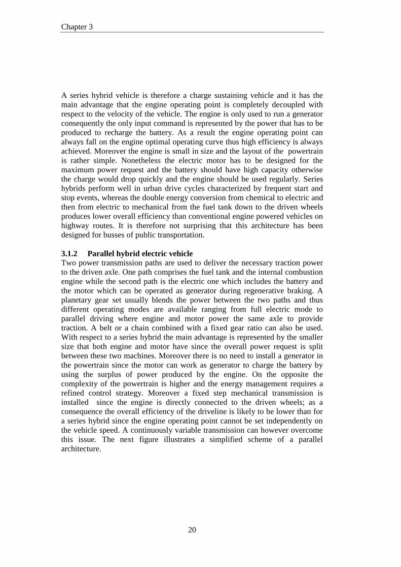
Chapter 3
20
A series hybrid vehicle is therefore a charge sustaining vehicle and it has the
main advantage that the engine operating point is completely decoupled with
respect to the velocity of the vehicle. The engine is only used to run a generator
consequently the only input command is represented by the power that has to be
produced to recharge the battery. As a result the engine operating point can
always fall on the engine optimal operating curve thus high efficiency is always
achieved. Moreover the engine is small in size and the layout of the powertrain
is rather simple. Nonetheless the electric motor has to be designed for the
maximum power request and the battery should have high capacity otherwise
the charge would drop quickly and the engine should be used regularly. Series
hybrids perform well in urban drive cycles characterized by frequent start and
stop events, whereas the double energy conversion from chemical to electric and
then from electric to mechanical from the fuel tank down to the driven wheels
produces lower overall efficiency than conventional engine powered vehicles on
highway routes. It is therefore not surprising that this architecture has been
designed for busses of public transportation.
3.1.2 Parallel hybrid electric vehicle
Two power transmission paths are used to deliver the necessary traction power
to the driven axle. One path comprises the fuel tank and the internal combustion
engine while the second path is the electric one which includes the battery and
the motor which can be operated as generator during regenerative braking. A
planetary gear set usually blends the power between the two paths and thus
different operating modes are available ranging from full electric mode to
parallel driving where engine and motor power the same axle to provide
traction. A belt or a chain combined with a fixed gear ratio can also be used.
With respect to a series hybrid the main advantage is represented by the smaller
size that both engine and motor have since the overall power request is split
between these two machines. Moreover there is no need to install a generator in
the powertrain since the motor can work as generator to charge the battery by
using the surplus of power produced by the engine. On the opposite the
complexity of the powertrain is higher and the energy management requires a
refined control strategy. Moreover a fixed step mechanical transmission is
installed since the engine is directly connected to the driven wheels; as a
consequence the overall efficiency of the driveline is likely to be lower than for
a series hybrid since the engine operating point cannot be set independently on
the vehicle speed. A continuously variable transmission can however overcome
this issue. The next figure illustrates a simplified scheme of a parallel
architecture.

Architectures of hybrid electric vehicles
21
Figure 3.2: Layout of the powertrain of a parallel HEV
Power flow is bidirectional in the electric path while energy recovery is
impossible through the engine. Thanks to the synergy of engine and electric
motor the driving range of parallel hybrids is longer than series hybrids.
Research around parallel hybrids is intensive since they represent a good
balance between driving range, reduction of pollutant emissions, fuel
consumption and driving performance. Several modifications to the basic layout
are available, for example transmission can be based on manual, automatic or
CVT. The rotor of the motor can be coupled to the driveshaft upstream or
downstream the transmission. Drivability issues like engine start&stop and gear
shift quality has to be taken into account when an energy management control
strategy is defined otherwise it can lead to poor on board comfort due to
excessive gear shifting or engine start&stop events.
3.1.3 Series/parallel hybrid electric vehicles
This configuration is regarded to as the most promising one since it collects the
advantages of series (the engine operating point is independent on the vehicle
speed) and parallel hybrids (synergy between engine and electric motor), giving
high flexibility of power management for better fuel economy. These
improvements are at the cost of higher complexity in the design and control of
the powertrain and also of higher cost of the vehicle for customers. Series-
parallel hybrids use extensively the engine in combination with the electric
machines but at the same time the engine operating point is decoupled from
vehicle speed; this enables to achieve high efficiency for all operating modes.
As for series hybrids an electric generator is added to the powertrain; it works as
starter for the engine and as source of electric energy to charge the battery when
it is commanded by the vehicle supervisory controller. It can also support the
engine and the electric motor to provide traction power for a limited time when
power request is very high. Series-parallel hybrid electric vehicles are
distinguished between power-split and 2x2. The next two figures report two
simplified schemes of the layout of the powertrain in these two cases.
Fuel tank
Engine
Battery Motor
Transmission
Ax
le
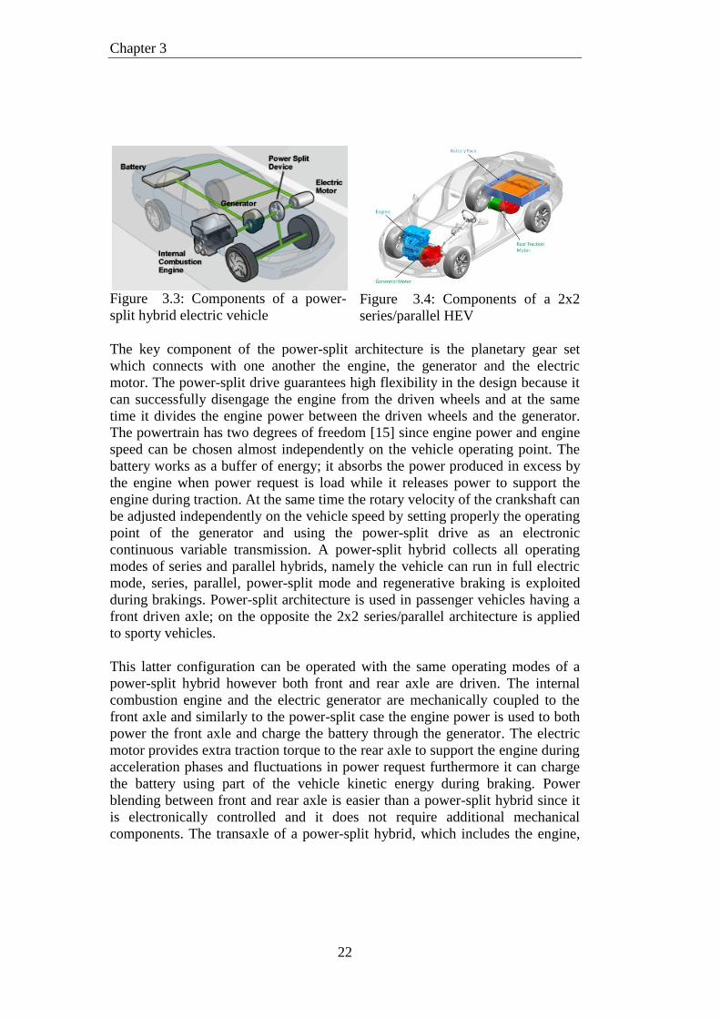
Chapter 3
22
Figure 3.3: Components of a power-
split hybrid electric vehicle
Figure 3.4: Components of a 2x2
series/parallel HEV
The key component of the power-split architecture is the planetary gear set
which connects with one another the engine, the generator and the electric
motor. The power-split drive guarantees high flexibility in the design because it
can successfully disengage the engine from the driven wheels and at the same
time it divides the engine power between the driven wheels and the generator.
The powertrain has two degrees of freedom [15] since engine power and engine
speed can be chosen almost independently on the vehicle operating point. The
battery works as a buffer of energy; it absorbs the power produced in excess by
the engine when power request is load while it releases power to support the
engine during traction. At the same time the rotary velocity of the crankshaft can
be adjusted independently on the vehicle speed by setting properly the operating
point of the generator and using the power-split drive as an electronic
continuous variable transmission. A power-split hybrid collects all operating
modes of series and parallel hybrids, namely the vehicle can run in full electric
mode, series, parallel, power-split mode and regenerative braking is exploited
during brakings. Power-split architecture is used in passenger vehicles having a
front driven axle; on the opposite the 2x2 series/parallel architecture is applied
to sporty vehicles.
This latter configuration can be operated with the same operating modes of a
power-split hybrid however both front and rear axle are driven. The internal
combustion engine and the electric generator are mechanically coupled to the
front axle and similarly to the power-split case the engine power is used to both
power the front axle and charge the battery through the generator. The electric
motor provides extra traction torque to the rear axle to support the engine during
acceleration phases and fluctuations in power request furthermore it can charge
the battery using part of the vehicle kinetic energy during braking. Power
blending between front and rear axle is easier than a power-split hybrid since it
is electronically controlled and it does not require additional mechanical
components. The transaxle of a power-split hybrid, which includes the engine,
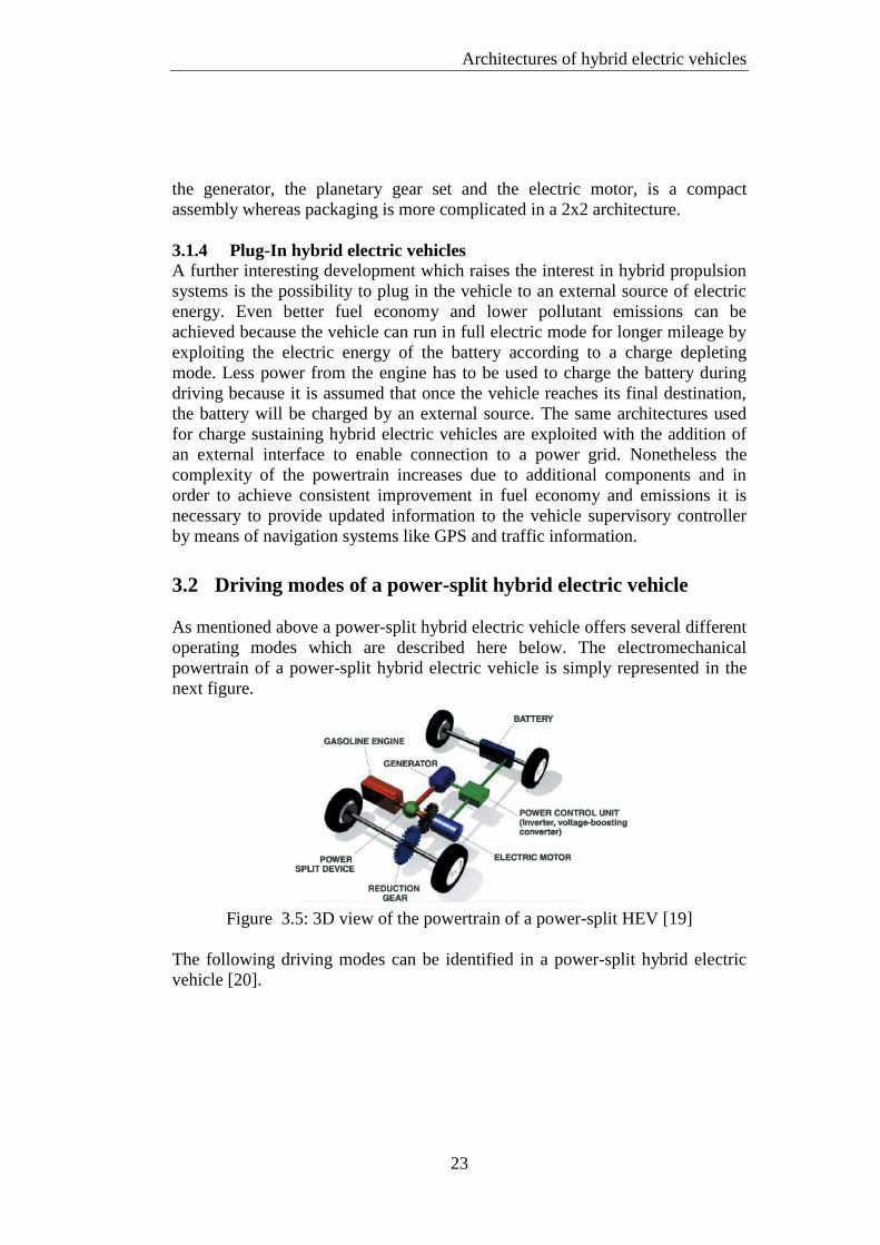
Architectures of hybrid electric vehicles
23
the generator, the planetary gear set and the electric motor, is a compact
assembly whereas packaging is more complicated in a 2x2 architecture.
3.1.4 Plug-In hybrid electric vehicles
A further interesting development which raises the interest in hybrid propulsion
systems is the possibility to plug in the vehicle to an external source of electric
energy. Even better fuel economy and lower pollutant emissions can be
achieved because the vehicle can run in full electric mode for longer mileage by
exploiting the electric energy of the battery according to a charge depleting
mode. Less power from the engine has to be used to charge the battery during
driving because it is assumed that once the vehicle reaches its final destination,
the battery will be charged by an external source. The same architectures used
for charge sustaining hybrid electric vehicles are exploited with the addition of
an external interface to enable connection to a power grid. Nonetheless the
complexity of the powertrain increases due to additional components and in
order to achieve consistent improvement in fuel economy and emissions it is
necessary to provide updated information to the vehicle supervisory controller
by means of navigation systems like GPS and traffic information.
3.2 Driving modes of a power-split hybrid electric vehicle
As mentioned above a power-split hybrid electric vehicle offers several different
operating modes which are described here below. The electromechanical
powertrain of a power-split hybrid electric vehicle is simply represented in the
next figure.
Figure 3.5: 3D view of the powertrain of a power-split HEV [19]
The following driving modes can be identified in a power-split hybrid electric
vehicle [20].
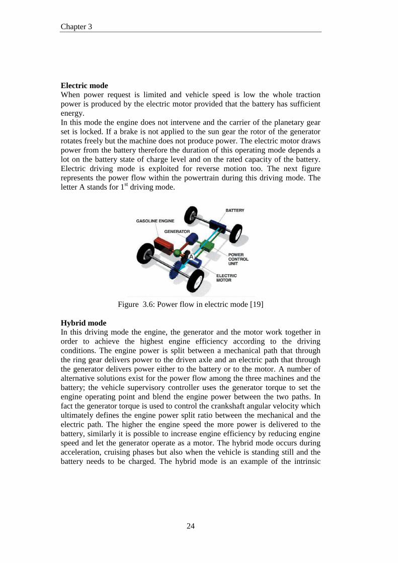
Chapter 3
24
Electric mode
When power request is limited and vehicle speed is low the whole traction
power is produced by the electric motor provided that the battery has sufficient
energy.
In this mode the engine does not intervene and the carrier of the planetary gear
set is locked. If a brake is not applied to the sun gear the rotor of the generator
rotates freely but the machine does not produce power. The electric motor draws
power from the battery therefore the duration of this operating mode depends a
lot on the battery state of charge level and on the rated capacity of the battery.
Electric driving mode is exploited for reverse motion too. The next figure
represents the power flow within the powertrain during this driving mode. The
letter A stands for 1st driving mode.
Figure 3.6: Power flow in electric mode [19]
Hybrid mode
In this driving mode the engine, the generator and the motor work together in
order to achieve the highest engine efficiency according to the driving
conditions. The engine power is split between a mechanical path that through
the ring gear delivers power to the driven axle and an electric path that through
the generator delivers power either to the battery or to the motor. A number of
alternative solutions exist for the power flow among the three machines and the
battery; the vehicle supervisory controller uses the generator torque to set the
engine operating point and blend the engine power between the two paths. In
fact the generator torque is used to control the crankshaft angular velocity which
ultimately defines the engine power split ratio between the mechanical and the
electric path. The higher the engine speed the more power is delivered to the
battery, similarly it is possible to increase engine efficiency by reducing engine
speed and let the generator operate as a motor. The hybrid mode occurs during
acceleration, cruising phases but also when the vehicle is standing still and the
battery needs to be charged. The hybrid mode is an example of the intrinsic
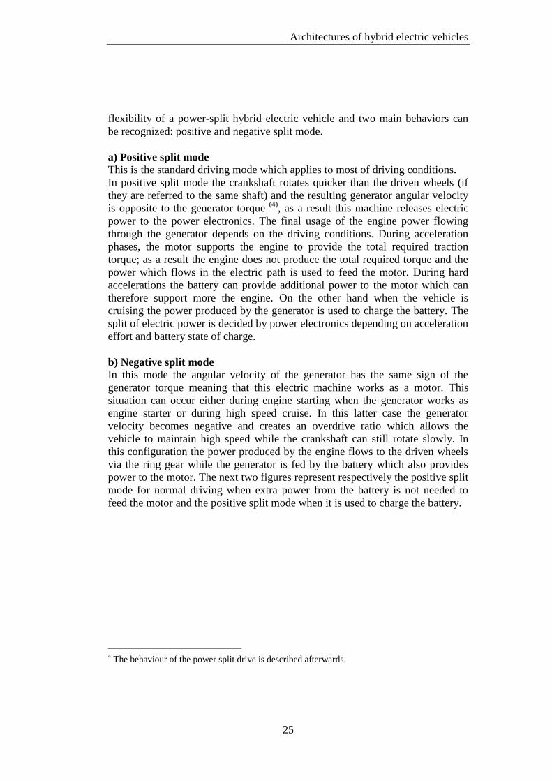
Architectures of hybrid electric vehicles
25
flexibility of a power-split hybrid electric vehicle and two main behaviors can
be recognized: positive and negative split mode.
a) Positive split mode
This is the standard driving mode which applies to most of driving conditions.
In positive split mode the crankshaft rotates quicker than the driven wheels (if
they are referred to the same shaft) and the resulting generator angular velocity
is opposite to the generator torque (4)
, as a result this machine releases electric
power to the power electronics. The final usage of the engine power flowing
through the generator depends on the driving conditions. During acceleration
phases, the motor supports the engine to provide the total required traction
torque; as a result the engine does not produce the total required torque and the
power which flows in the electric path is used to feed the motor. During hard
accelerations the battery can provide additional power to the motor which can
therefore support more the engine. On the other hand when the vehicle is
cruising the power produced by the generator is used to charge the battery. The
split of electric power is decided by power electronics depending on acceleration
effort and battery state of charge.
b) Negative split mode
In this mode the angular velocity of the generator has the same sign of the
generator torque meaning that this electric machine works as a motor. This
situation can occur either during engine starting when the generator works as
engine starter or during high speed cruise. In this latter case the generator
velocity becomes negative and creates an overdrive ratio which allows the
vehicle to maintain high speed while the crankshaft can still rotate slowly. In
this configuration the power produced by the engine flows to the driven wheels
via the ring gear while the generator is fed by the battery which also provides
power to the motor. The next two figures represent respectively the positive split
mode for normal driving when extra power from the battery is not needed to
feed the motor and the positive split mode when it is used to charge the battery.
4 The behaviour of the power split drive is described afterwards.

Chapter 3
26
Figure 3.7: Positive split mode. C and
B mark two paths for engine power to
the wheels [19].
Figure 3.8: Positive split mode. the
engine power is used to charge the
battery [19].
Parallel mode
The sun gear can be locked by means of a brake and thus the rotor of the
generator cannot rotate. In this situation the whole engine power is delivered to
the driven axle which represents a more efficient operating condition rather than
delivering power to the wheels via the generator and the motor. This operating
mode is mostly applied when the vehicle is being driven at rather high constant
velocity; a null generator angular velocity helps to keep the crankshaft angular
velocity low and therefore to make the engine operate in a region of high
efficiency. The motor can support the engine either with a positive torque to
cope with an increase in power request by drawing energy from the battery or
with a negative torque to absorb the extra torque produced by the engine. Again
the battery provides an additional degree of freedom to achieve higher fuel
economy than a conventional vehicle. The power flow is equal to the case of
positive split mode except for the fact that the entire engine power flows to the
driven axle.
Regenerative braking
During braking, part of vehicle kinetic energy can be recovered at the axle
powered by the electric motor by using this machine as generator. For a power-
split architecture the motor powers the front axle and during regenerative
braking the engine rotates freely meaning that no power flows in the planetary
gear set. The motor can therefore absorb power and deliver it to the battery to
replenish the state of charge.

Architectures of hybrid electric vehicles
27
Figure 3.9: Regenerative braking. Part of vehicle’s kinetic energy is recovered
in the high voltage battery [19].
Engine braking
During long braking on strongly inclined road or when the battery is
overcharged and regenerative braking cannot be carried out, engine braking is
accomplished. In this mode the motor does not apply any load to the axle and
rotates freely while the engine is idling and absorbs power. Again the engine
speed is controlled according to the vehicle speed in order to set the amount of
power that should be absorbed. Conventional service braking system can
intervene during both regenerative braking and engine braking to add an
additional braking torque.
3.3 Main components of the analyzed HEV
A power-split hybrid electric vehicle has been analyzed deeply through a high
fidelity model implemented in Amesim®. The Amesim
® model represents the
architecture of a front wheel drive power-split powertrain whose architecture
resembles the one represented in Figure 3.5 even if the model includes a silent
chain in-between the front axle and the ring gear. Consequently the final
transmission introduces a fixed gear ratio, which is obtained as the series of the
silent chain and the set of gear wheels, but also it adds elasticity and damping to
the driveline. The engine, the power split drive, the electric machines and the
battery are the most important components in the powertrain for this reason their
properties are introduced now, while the vehicle assembly is treated afterwards.
3.3.1 Power-split drive
The next figure illustrate a planar view of the transaxle of a common power-split
hybrid electric vehicles which comprise the three power units and the planetary
gear set or power-split drive.
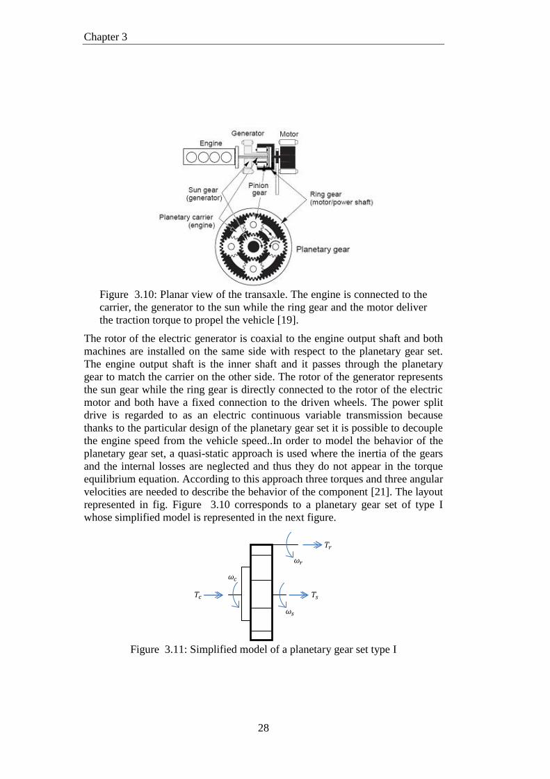
Chapter 3
28
Figure 3.10: Planar view of the transaxle. The engine is connected to the
carrier, the generator to the sun while the ring gear and the motor deliver
the traction torque to propel the vehicle [19].
The rotor of the electric generator is coaxial to the engine output shaft and both
machines are installed on the same side with respect to the planetary gear set.
The engine output shaft is the inner shaft and it passes through the planetary
gear to match the carrier on the other side. The rotor of the generator represents
the sun gear while the ring gear is directly connected to the rotor of the electric
motor and both have a fixed connection to the driven wheels. The power split
drive is regarded to as an electric continuous variable transmission because
thanks to the particular design of the planetary gear set it is possible to decouple
the engine speed from the vehicle speed..In order to model the behavior of the
planetary gear set, a quasi-static approach is used where the inertia of the gears
and the internal losses are neglected and thus they do not appear in the torque
equilibrium equation. According to this approach three torques and three angular
velocities are needed to describe the behavior of the component [21]. The layout
represented in fig. Figure 3.10 corresponds to a planetary gear set of type I
whose simplified model is represented in the next figure.
Figure 3.11: Simplified model of a planetary gear set type I

Architectures of hybrid electric vehicles
29
The following kinematic relationship holds for the three angular velocities.
(3.1)
The sun gear, the carrier and the ring gear are parallel and coaxial therefore the
following torque equilibrium holds:
(3.2)
Assuming no power loss inside the planetary gear set, the inlet power flow has
to be balanced by the outlet power flow as follows:
(3.3)
By rearranging the set of equations (3.1), (3.2), (3.3) it is possible to express the
angular velocity of the carrier and the outlet torque at the ring gear and at the
carrier as function of the angular velocity of the ring gear, sun gear and the inlet
torque at the sun gear.
(3.4)
The angular velocity of the carrier corresponds to the angular velocity of the
crankshaft while the angular velocity of the ring is related to the vehicle speed
through a fixed gear ratio, therefore the angular velocity of the generator can be
used to decouple these two former variables and thus it enables to achieve
higher efficiency of the engine. In practice the engine is speed controlled
meaning that the generator torque is used to set the desired angular velocity of
the crankshaft. The planetary gear set that is modeled here has the following
characteristics:

Chapter 3
30
3.3.2 Internal combustion engine
The vehicle is equipped with a 1.2 liters gasoline atmospheric engine.
This gasoline engine produces a maximum torque of 174 Nm at 4500 rpm and
delivers a maximum output power of 89.21 kW at 5000 rpm. The characteristic
curves of engine torque are defined by means of tables as well as the fuel mass
flow rate; the next two figures report respectively a contour plot of the fuel mass
flow rate as function of the engine operating point and the engine characteristic
curves. The engine Optimal Operating Line is defined as the set of operating
points which release a given power with the lowest fuel mass flow rate; this
curve is also represented in the next figures by means of a green piecewise
linear envelope.
Figure 3.12: Fuel mass flow rate [g/s]
as function of engine torque and
speed. The engine OOL is the green
curve.
Figure 3.13: Characteristic curves of
the engine. Maximum, minimum
torque and engine OOL.
The torque that the engine can produce at a given angular velocity of the
crankshaft is controlled by the admission rate or engine load. Negative torques
are controlled by values of the engine load between and where
corresponds to the minimum curve. A load equal to 1 defines the
maximum achievable engine torque while all other torque values are obtained as
linear interpolation between these two curves for a specific value of the engine
speed. Negative engine torques represent friction and pumping losses inside the
combustion chamber. The engine output torque is calculated from a value read
in a table which is modified by a first order dynamics in order to take into
account the delay in engine response. The value from the table is read as
function of engine admission rate and input engine speed; this value is modified
in order to take into account possible variation of air density in comparison to
the default value and the time lag due to the combustion process. Consequently
the engine torque delivered at the crankshaft is obtained as a result of these two
subsequent steps:

Architectures of hybrid electric vehicles
31
where is while is equal to
Similarly the fuel mass flow rate and the pollutant emission rates are read from
correspondent tables as function of the engine operating point.
These output values are modified according to the engine wall temperature in
case a thermal management analysis is carried out. In this thesis work the engine
wall temperature and the cooling fluid temperature are kept constant throughout
the simulations consequently these changes are not applied; similarly the air
density is set equal to its default value so it does not introduce any additional
changes.
3.3.3 Electric machines
The generator and the electric motor are represented by the same type of electric
machine; this designing solution holds for many series-parallel hybrid vehicles
on the market since it reduces the production costs. The functionalities of the
machine is described by means of tables and equations; in particular a table
contains the maximum torque values as function of the rotor angular velocity
and the input voltage while the power losses are expressed as function of the
operating point (torque and speed) of the machine. The following two figures
illustrate the characteristic curve of the electric machines and the power loss as
function of the operating point.

Chapter 3
32
Figure 3.14: Output torque as
function of input voltage and rotor
angular velocity.
Figure 3.15: Power losses as function
of output torque, rotor angular
velocity [19].
The characteristic curve of the electric machines is expressed as function of
input voltage and angular velocity of the rotor. The torque value obtained from
the table is applied to the powertrain according to a first order dynamics which
is meant to model the time delay that is always present in a real machine. This
first order dynamics and the table substitute the power electronics that control a
real electric machine but which are not included in this model.
The output shaft torque is calculated as follows:
where is equal to 0.001s
The electric machines are connected to the battery via electric coils and set the
electric load for the battery while this latter defines the input voltage to the
machine. The rotary inertia of the rotor is simply modeled through a 1D disc
which is placed downstream the electric machine.
3.3.4 High voltage battery
A hybrid electric vehicle is equipped with two batteries. The high voltage
battery is involved in the power management of the vehicle while a 12V battery
feeds few auxiliary components. Regarding the energy management only the
high voltage battery is important and in the following this component is named
simply as battery. The battery is modeled as an assembly of equivalent electric
circuits [21] where each circuit represents a single cell of the battery. The
internal properties of internal resistance and open circuit voltage of the battery
are determined by the arrangement of the cell banks which can be placed in
parallel and in series together with additional data which describe these
variables as functions of the battery internal fluid temperature and the battery
state of charge. The next figures illustrate an example of banks arrangement
with 4 banks in series, 7 banks in parallel and 3 cells per battery bank; moreover

Architectures of hybrid electric vehicles
33
the equivalent electric circuit that is used to model a cell of the battery is shown
too.
Figure 3.16: Arrangement of battery banks. Equivalent electric circuit of a
single battery cell [19].
Each cell is modeled as an equivalent electric circuit with an internal resistance
and a voltage source represented by the open circuit voltage.
The equation of the circuit can be written as follows:
(3.5)
The values of and are read from correspondent tables as function of
battery state of charge and battery internal temperature. Throughout the analysis
none temperature change has been considered hence the temperature has been
kept constant to 80°C. The next two figures represent the values of the two
parameters as function of temperature and depth of discharge which is defined
as – .
Figure 3.17: Internal resistance of a
cell as function of state of discharge
and temperature.
Figure 3.18: Open circuit voltage of a
cell as function of state of discharge
and temperature.
Under the assumption that the cells behave in the same way, it is possible to
obtain the battery output quantities from the electric behavior of a single cell and
the banks arrangement. As a result the battery total current, the battery output
voltage and the battery total resistance are calculated as follows:

Chapter 3
34
(3.6)
The battery open circuit voltage is defined through the following equation:
(3.7)
The battery total current is negative when the battery discharges as a
consequence the time derivative of the battery charge is defined as follows:
(3.8)
By comparing this time derivative with the battery rated capacity it is possible to
define the time derivative of the battery state of charge as a function of the
battery load:
(3.9)
3.3.5 The vehicle assembly
The vehicle assembly comprises the wheels, the suspension system and the
carbody. The torque delivered by the driveline is applied to the driving wheels
which are characterized by a rotary inertia while the tyre properties are modeled
by means of Pacejka 89. The wheel normal load is a function of the carbody
pitch motion and it is used inside the Pacejka model. The wheels are connected
to the carbody via the suspension assembly which comprises for each axle an
unspung mass, tyre and suspension stiffness, viscous dampers. The carbody is
subjected to the aerodynamic drag and to the reaction torques and forces from
the engine block, suspension system. The engine block is connected to the
chassis by means of three bushings thus the model computes the transmissibility
of forces and oscillations between the engine and the carbody. The overall
dynamics in the vehicle symmetry plane is solved by using the Euler equations,
while the vehicle lateral dynamics is not analyzed in this model.
The nominal values of the most important parameters which characterize the
vehicle are provided in the following list:
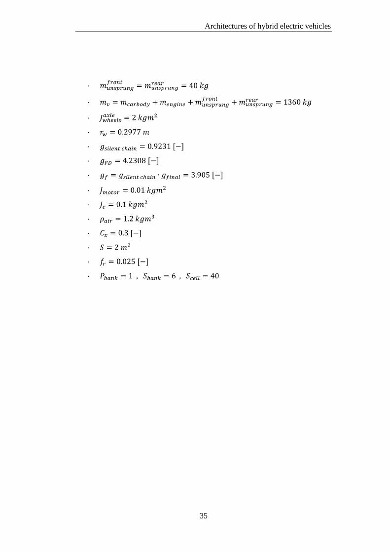
Architectures of hybrid electric vehicles
35

Chapter 3
36
37
4 The MPC-based control strategy
In this chapter it is described how predictive control can be used to develop a
control strategy which manages the power split of a hybrid electric vehicle in
order to achieve the desired objectives. Model predictive control relies on a
mathematical formulation of the system, thus the chapter illustrates the physical
and mathematical modeling that has been applied to set up the optimization
problem in order to calculate the optimal control strategy.
4.1 Background
In chapter 2 it is underlined how the energy management of a hybrid electric
vehicle can be formulated as a constrained optimization problem whose solution
is generally computed by means of numeric algorithms. Different approaches
have been tested so far to get a suitable optimal control action and Model
Predictive Control (MPC) is included in this list. Model Predictive Control
belongs to the family of model based optimal control theory where a numeric
optimization problem is solved to compute the control action which can drive a
dynamic system to a desired set point while achieving the best performance
defined by a proper index. In fact a system usually has to be driven to a desired
set point starting from an initial configuration. The trajectory that the system can
follow from this initial state to the final desired one is usually constrained by a
number of state constraints; however even in this situation there is normally a
bunch of alternative control actions which can lead the system to the final state.
Each control action makes the system follow a different trajectory once it is
applied. Besides the desired final set point additional requests are usually
specified on some performance that the system should achieve while moving
along a trajectory; therefore the control action which can achieve the best
performance indices is the optimal one and it is the only one which should be
applied to the system. Model Predictive Control computes this optimal control
strategy by combining predictions of future system response to an optimization
problem. A simple example is described below to clarify the operating principle
of MPC.

Chapter 4
38
Figure 4.1: (a). (left) A system may move from Xo to XN following three
possible different trajectories. (b) (middle) the constraints are dynamic and the
optimal trajectory needs to be recomputed. (c) (right) MPC updates the optimal
control action at each sampling time.
Figure 4.1(a) represents the initial state and the desired set point that the
system is supposed to achieve, while the blue circles represent the state
constraints. MPC knows the initial and the desired final states moreover it
includes models of the dynamics of the system and of the shape of the
constraints. Using these models MPC can formulate three suitable control
actions and by using the model of the system dynamics it can predict the
correspondent trajectories that the system would follow once these control
sequences were applied to the system. The three trajectories are represented in
Figure 4.1(a) with blue, purple and red colours. In this example it is supposed
that the control actions are defined in order to bring the system to the final state
however in the classical MPC formulation the prediction can be limited to few
future steps and thus the control action is meant to bring the system to an
intermediate future state.
Suppose the performance index were the minimization of the total travel
distance, then the trajectory represented in blue would minimize this objective
while satisfying all constraints, thus the correspondent control action would be
the optimal one. This optimal control action is calculated as the solution of a
constrained mathematical optimization problem where the objective function to
be minimized corresponds to the total travel distance from to . Figure
4.1(b) shows that the state constraints are dynamic hence they change while the
system evolves from to under the input . Therefore if the control action
were not changed the system would violate one or more constraints along its
trajectory. This is not an issue for MPC since it samples the new operating
conditions of the system at and updates the model of the constraints, thus it
can compute a new optimal control action to drive the system from to by
solving a new optimization problem. Once the system gets to the whole
optimization problem is repeated once more in order to calculate a new optimal
control action to drive the system from to . This procedure is repeated

The MPC-based control strategy
39
even if the constraints do not alter their shape and thus the optimal control
action defined at the previous step would still match the requests. Consequently
MPC calculates by nature a feed forward control action which would bring the
system from the given state to the final desired one however only the first
element of the computed control sequence is applied to the system and then the
optimization problem is repeated at the next sampling time using as inputs the
new operating conditions and moving the prediction horizon one step forward.
This approach is called receding horizon and it brings to a feedback control
action.
This simple example highlights the core points of MPC:
Reference model of the system: a model of system dynamics is used to
predict its response under the effect of a control action and known
external disturbances.
Model of the constraints: it evaluates the prediction of system response
against the constraints in order to understand if a control action would
bring the system to an unfeasible operating condition.
Objectives: typically a desired final state should be achieved, in parallel
some performance indices should be either maximize or minimize, for
example travel time or distance.
Optimization: a constrained optimization problem is solved in order to
calculate the optimal control action which can successfully drive the
system to the desired state while satisfying all constraints and achieving
the best performance according to the objectives.
From the example above it is clear that the optimization problem should be
solved numerically through a sequence of iterations which tries to diminish the
cost function until its global optimum. However an optimization problem has
generally many local minima and during the course of the optimization routine
the algorithm may stuck in a local minimum without getting to the global
optimum of the cost function. A convex optimization problem does not suffer
from this drawback since convexity of the cost function assures that just one
point of minimum exists thus the algorithm would reach this point provided that
it converges successfully. A Quadratic Programming problem where the cost
function is a quadratic function of the control variables while the constraints are
linear functions of the control variables, is desirable for MPC application since it
MPC
Model Constraints
Objectives Optimization

Chapter 4
40
guarantees convexity of the optimization problem provided that few conditions
are satisfied by the cost function and the constraints. There exist a number of
efficient algorithms that have been developed to solve specifically quadratic
programming problems hence the optimal solution can usually be computed
quickly. Therefore the aim is to set up the optimization problem as a QP
problem and the four core points should have a proper mathematical
formulation. The remaining part of the chapter describes the mathematical
procedures that are necessary to compute a suitable MPC-based control strategy
for the energy management of a power-split hybrid electric vehicle, the
conditions which guarantee the convexity are highlighted.
4.2 Formulation of the MPC strategy
4.2.1 The reference simplified model
The reference model should be simple to reduce the computational effort of the
optimization problem but at the same time it should be reliable to guarantee a
correct prediction of future responses of the system to input control commands
and know external disturbances. In order to develop a state space form which
enables the definition of a model based optimal control strategy a forward
approach has been applied besides a quasi-static modeling of most of the
powertrain components [21]. Forward approach has been used to model the
longitudinal motion of the vehicle. According to this approach the actual vehicle
speed is compared to the desired vehicle speed and the error is used by a PID
controller to generate proper control commands. The PID controller models the
driver and the output commands are sent to the components of the powertrain in
order to generate the necessary tractive or braking torque to track the reference
velocity profile. The driveline output torque is applied to the vehicle and the
output of the simulation is the vehicle speed obtained from integration of the
vehicle longitudinal dynamics. On the contrary a backward approach would
assign the reference velocity profile as input and the equation of the vehicle
longitudinal motion is used to calculate the correspondent torques produced by
the engine and the electric machines, hence the outcomes of the simulation are
the fuel consumption and the battery state of charge.
The forward approach is more realistic and is preferable when a control strategy
is designed since it permits to evaluate the stability of the strategy because the
commands produced by the driver are not known a priori. Moreover a backward
approach assumes that the powertrain can always match instant by instant the
desired velocity profile which is not generally true when the torque request
exceeds the powertrain limits. Consequently the simple reference model is
obtained under the assumption that the driver provides as input the desired
torque request in order to track the reference velocity profile while the control

The MPC-based control strategy
41
strategy provides the control commands to the prime movers to match the torque
and power request from the driver. Both the driver and the control strategy are
outside the reference model even if the MPC-based control strategy uses this
latter model to predict the response of the powertrain to a specific control action.
The behavior of the components of the powertrain has been modeled either as
quasi-static or as dynamic. In a dynamic approach the behavior of a component
is modeled through a differential equation or a set of differential equations; this
enables to capture high frequency dynamics of the component. On the other
hand a quasi-static approach neglects any dynamics associated to the behavior of
a component and the modeling exploits only equilibrium equations.
Eventually the following assumptions have been considered to derive the model:
the dynamics associated to the rotary motion of the rotor of the generator
and the rotor of the motor are much faster compared to the first rotary
dynamics of the crankshaft and the response of the vehicle regarding its
longitudinal motion. As a result the rotary inertia of the generator and the
motor have been neglected.
the engine block is assumed to be rigidly connected to the carbody
meaning that the bushings are neglected and the inertia of the engine
block is included in the inertia of the carbody. On the other hand the
flywheel is modeled through a rotary inertia.
the transmission (planetary gear set, final gear ratio and front
differential) is assumed to have unitary efficiency.
the rotary inertia of all components in the transmission is neglected.
temperature effects are neglected
the battery is modeled by means of an equivalent electric circuit
damping, flexibility along the transmission and in the suspension
assembly are neglected
no tyre model is introduced. It is assumed that both the traction torque
delivered by the driveline and the braking torque can always be
immediately and completely discharged to the ground
wind velocity and road slope are not considered since their values cannot
be known by the MPC controller at this stage
the rotary inertia of the four wheels is replaced by an equivalent linear
inertia which augments the overall vehicle mass in the differential
equation which describes the longitudinal motion of the vehicle
the vehicle dynamics is solely described regarding the longitudinal
motion of the vehicle, thus neither bounce nor pitch nor yaw motion is
treated by this simplified model. As a consequence the effect of mass
transfer on vehicle dynamics is neglected.
similarly to the previous point the actual braking force distribution
between the front and the rear axle is neglected and the total braking
torque is assumed to be applied at the driven axle.

Chapter 4
42
the total braking torque is split between the torque provided by the
service braking system and the torque obtained through regenerative
braking at the front axle by using the motor as electric generator.
the four wheels are merged together into a single wheel which combine
the overall rotary inertia.
the longitudinal dynamics of the vehicle is described as the motion of a
point mass subjected to resistive forces given by rolling resistance,
braking torque and air resistance together with a traction effort produced
by the powertrain
the only available information on driving conditions are represented by
the driver’s torque request and the vehicle actual longitudinal velocity at
the sampling time.
For the energy management problem the dynamics of the battery state of charge
is generally the only state variable that is taken into account, however the MPC
strategy has been developed in order to address simple issues related to on-board
comfort therefore the angular velocity of the crankshaft has been used as second
state of the system. This choice comes mainly from [18] and from preliminary
observations done besides some simulations carried out with the original rule
based strategy. In these simulations it appears that every time the engine is
activated or stopped the carbody experiences large oscillations of longitudinal,
vertical and pitch accelerations due to a quick variation of generator torque
which has the task to adjust the angular velocity of the crankshaft. In order to
overcome this issue the rotary inertia of the crankshaft is introduced to define
the engine torque and the generator torque as control inputs and thus smooth the
action of this latter variable. If the dynamics of the crankshaft were not
considered, then the engine and the generator torques would be simply related
by an equilibrium equation and it would not be possible to achieve a smooth
engine starting and stopping inside the control strategy itself. Considering these
assumptions, the powertrain can be modeled using two separate models for the
mechanical and the electrical side. These two sides can communicate through
the battery power.

The MPC-based control strategy
43
Electric side
The pure electric side of the system is represented by the battery. The simplest
battery model is an equivalent electric circuit characterized by a total internal
resistance and an overall open circuit voltage. The scheme of this circuit is
reported in the next figure.
Figure 4.2: Equivalent electric circuit which models the battery
Applying the Kirchhoff’s circuit law, the voltage equilibrium produces the
following relation:
(4.1)
In a battery power is lost due to electric and chemical processes; it is assumed
that the equivalent internal resistance collects all these losses. Multiplying the
latter equation on both sides by the battery output voltage and rearranging the
terms, produces:
(4.2)
(4.3)
The only feasible solution is the one with sign “+” because when electric current
does not flow in the circuit the output voltage equates the open circuit voltage.
By replacing this latter equation into the definition of the battery output current
and by transforming the denominator using the rationalization formula, it
results:
(4.4)

Chapter 4
44
The time derivative of the battery state of charge is defined as the ratio of the
battery output current over the battery rated capacity, where positive current
indicates that the battery is discharging power:
(4.5)
As a result the time derivative of the battery state of charge depends on the
electric load acting on the battery, this load is defined by the battery power
which corresponds to the summation of the power associated to the generator,
motor and power losses inside these machines as follows.
(4.6)
Power losses are always positive while electric power associated to the
operating points of the machines can assume both positive and negative values
as a consequence the electric machines can either draw of provide power to the
battery. Since the electric machines contribute to produce the tractive force they
are included in the mechanical side of the powertrain and thus the battery power
is the variable which connects the two sides of the powertrain.
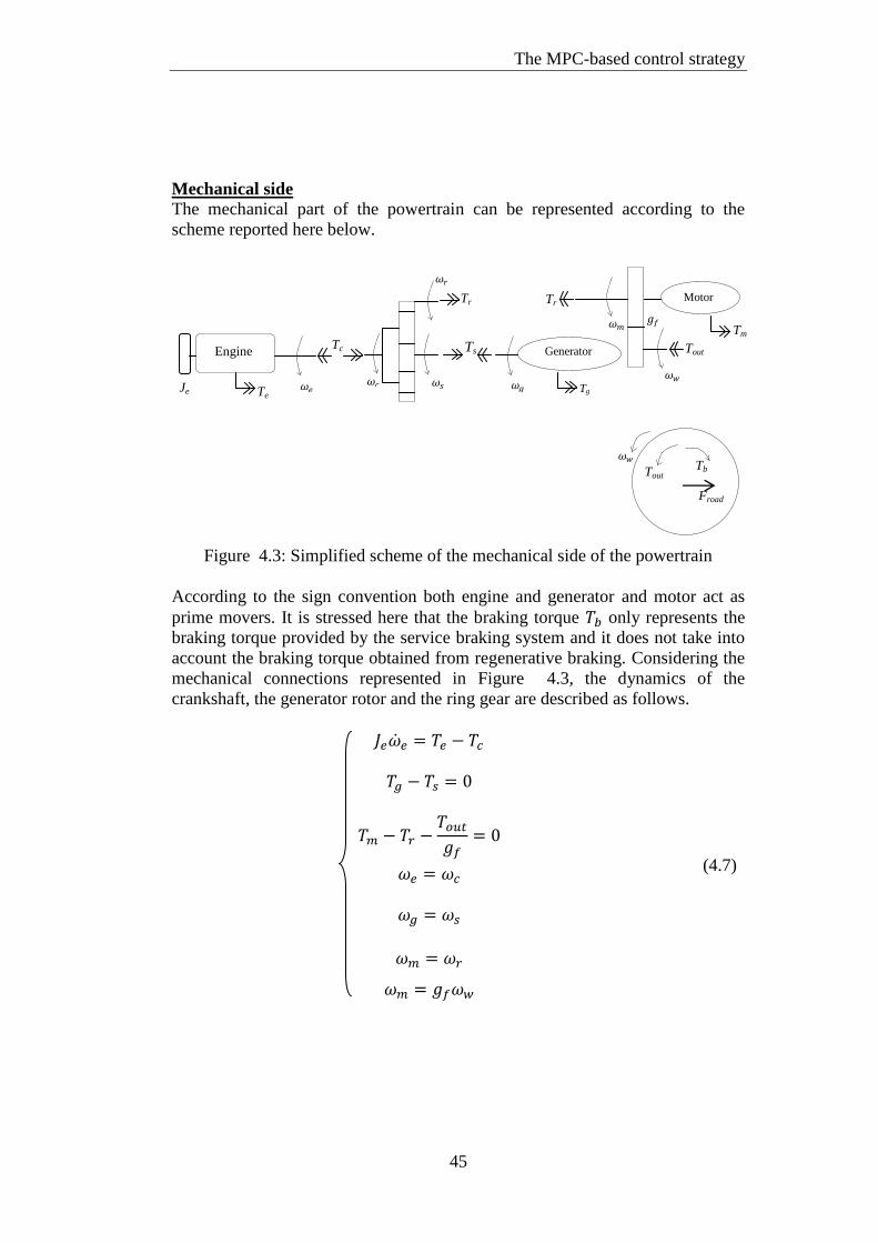
The MPC-based control strategy
45
Mechanical side
The mechanical part of the powertrain can be represented according to the
scheme reported here below.
Figure 4.3: Simplified scheme of the mechanical side of the powertrain
According to the sign convention both engine and generator and motor act as
prime movers. It is stressed here that the braking torque only represents the
braking torque provided by the service braking system and it does not take into
account the braking torque obtained from regenerative braking. Considering the
mechanical connections represented in Figure 4.3, the dynamics of the
crankshaft, the generator rotor and the ring gear are described as follows.
(4.7)
Engine Generator
Motor
Te
Tc
Tr Tr
Ts
Tg
Tm
Tout
Tout Tb
Froad
Je

Chapter 4
46
Subsequently by neglecting any rotary inertia and friction loss inside the power
split drive, by combining the governing equations (3.4) with equations (4.7) the
following relations are determined.
(4.8)
Applying the longitudinal force equilibrium at the driven wheels, the governing
differential equation of the vehicle longitudinal motion can be written as
follows:
(4.9)
An important assumption is introduced at this point regarding the torque
equilibrium along the driveline. The driveline is assumed to be able to satisfy
the torque required by the driver meaning that the torque delivered by the
driveline equates the torque required by the driver. As a result the torque
required by the driver is treated as an external disturbance which is known at the
sampling time and thus the vehicle velocity can be integrated using equation
(4.9) once the driveline output torque and the braking torque are replaced by the
torque required by the driver as follows.
(4.10)
The driver’s desired torque and the vehicle longitudinal velocity represent the
known external disturbances applied to the system and they can be introduced in
equations (4.8) as known variables so that the generator angular velocity, the
motor angular velocity and the motor torque can be expressed as follows:

The MPC-based control strategy
47
(4.11)
If the battery state of charge and the crankshaft angular velocity represent the
states of the system, the engine torque, the generator torque and the total braking
torque provided by the service braking system represent the control inputs then
the following nonlinear state space form can be defined:
(4.12)
where:
The nonlinear state space form in (4.12) provides the description of the time
derivatives of the states as function of system states themselves, control inputs
and external measured disturbances; however up to this point some variables are
related to by means of look-up tables.

Chapter 4
48
For example the fuel mass flow rate in the output equations is described by a
Multi 1D table as function of engine speed and torque, similarly the power loss
inside an electric machines is described by a look-up table as function of the
operating point of the machine as described in Chapter 3.3.3. In order to
overcome this issue each look-up table has been replaced by a regression model
because the control strategy can handle a continuous mathematical function
better than a look-up table. Four regression surfaces have been obtained to
describe respectively fuel mass flow rate, power losses in the electric machines,
battery open circuit voltage and internal resistance of a single cell. The post
processing of the experimental data and the mathematical procedure that has
been followed to compute the regression models is reported below.
Fuel mass flow rate The available data have been modified due to the fact that:
11 curves are provided where each curve reports the fuel mass flow
rate as function of a set of values of engine torque and for a specific
value of crankshaft angular velocity. 11 different angular velocities
have been tested. A problem is represented by the fact that each
curve has been obtained for a different number of engine torque
samples; moreover the engine torque values that have been tested are
different from test to test. While a single vector of angular velocity
values is available, there are 11 available vectors of engine torque
levels. Therefore a new grid of experimental values of engine speed
and torque has been defined starting from the available data.
Fuel consumption is not given for null and negative values of engine
torque
Torque is expressed as break mean equivalent pressure BMEP [bar]
and fuel consumption as g/kWh.
Engine torque can be expressed in [Nm] using the following definition of the
BMEP:
(4.13)
where T indicates the engine torque in Nm.
Fuel consumption can be expressed in [g/s] by multiplying the value in g/kWh
times the power produced by the engine at a correspondent operating point on a
curve:
(4.14)
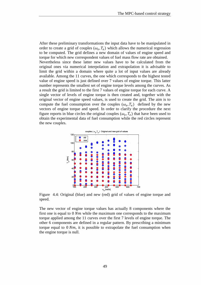
The MPC-based control strategy
49
After these preliminary transformations the input data have to be manipulated in
order to create a grid of couples ( which allows the numerical regression
to be computed. The grid defines a new domain of values of engine speed and
torque for which new correspondent values of fuel mass flow rate are obtained.
Nevertheless since these latter new values have to be calculated from the
original ones via numerical interpolation and extrapolation it is advisable to
limit the grid within a domain where quite a lot of input values are already
available. Among the 11 curves, the one which corresponds to the highest tested
value of engine speed is just defined over 7 values of engine torque. This latter
number represents the smallest set of engine torque levels among the curves. As
a result the grid is limited to the first 7 values of engine torque for each curve. A
single vector of levels of engine torque is then created and, together with the
original vector of engine speed values, is used to create the grid. The aim is to
compute the fuel consumption over the couples ( defined by the new
vectors of engine torque and speed. In order to clarify the procedure the next
figure reports in blue circles the original couples ( that have been used to
obtain the experimental data of fuel consumption while the red circles represent
the new couples.
Figure 4.4: Original (blue) and new (red) grid of values of engine torque and
speed.
The new vector of engine torque values has actually 8 components where the
first one is equal to while the maximum one corresponds to the maximum
torque applied among the 11 curves over the first 7 levels of engine torque. The
other 6 components are defined in a regular pattern. By prescribing a minimum
torque equal to , it is possible to extrapolate the fuel consumption when
the engine torque is null.

Chapter 4
50
The new values of fuel consumption have been obtained by interpolation and
extrapolation of the original values over the new values of engine torque for
each given experimental curve. In order to obtain good results, spline functions
have been used for both interpolation and extrapolation. Regarding extrapolation
of fuel consumption at null engine torque, spline functions have been used but
only the first 4 points of each curve have been considered. This is because a
better trend can be obtained close to the null torque when fewer points are
considered. The next two figures summarize these steps; Figure 4.5 represents
the 11 experimental curves that are provided whereas Figure 4.6 reports an
example of interpolation and extrapolation of fuel consumption values over the
new values of engine torque and for curve number 8. The blue circles represent
the original values while the red circles the new ones. In this latter figure fuel
consumption for null torque is still equal to ; this is because the
extrapolation to determine fuel consumption for null engine torque is carried out
afterwards.
Figure 4.5: 11 Experimental curves
which represent fuel mass flow rate as
function of engine speed and engine
torque.
Figure 4.6: An example of
interpolation of fuel consumption over
the new set of engine torque values for
curve number 8.
An analysis of the regression surface obtained after some preliminary trails has
shown how assuming a small but not null fuel consumption value for null engine
torque improves a lot the quality of the regression over the whole
domain . Consequently spline functions extrapolate this value for each
curve.
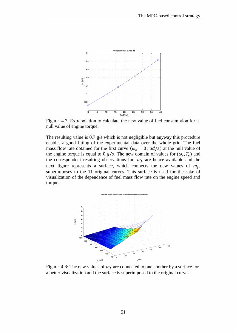
The MPC-based control strategy
51
Figure 4.7: Extrapolation to calculate the new value of fuel consumption for a
null value of engine torque.
The resulting value is 0.7 g/s which is not negligible but anyway this procedure
enables a good fitting of the experimental data over the whole grid. The fuel
mass flow rate obtained for the first curve at the null value of
the engine torque is equal to . The new domain of values for ( and
the correspondent resulting observations for are hence available and the
next figure represents a surface, which connects the new values of ,
superimposes to the 11 original curves. This surface is used for the sake of
visualization of the dependence of fuel mass flow rate on the engine speed and
torque.
Figure 4.8: The new values of are connected to one another by a surface for
a better visualization and the surface is superimposed to the original curves.

Chapter 4
52
This surface suggests that fuel flow rate can be related to engine speed through a
quadratic function while a higher order relation may explain fuel mass flow rate
with respect to engine torque. Regression analysis reveals that the following
polynomial expression fits well the new observed values; in [Nm], in
[rad/s] while in [g/s]:
(4.15)
In order to assess the quality of the regression model the surface has been
extended to those points which lie outside the considered domain, namely for
engine torque values higher than 72 Nm, and then it has been compared to those
few experimental values that are available at these higher torque levels.
The next figure reports a visual comparison.
Figure 4.9: Polynomial regression model of fuel flow rate over the entire
operating domain of the engine.
The surface fits the experimental data reasonably well even outside the domain
used to derive the regression model, thus a new set of regressors has been
calculated using an algorithm for global optimization and extending the
minimization of the sum of the quadratic residuals over the entire domain
defined by the original couples . The regression is poorer when both
engine speed and torque assume high values. In this area the surface
overestimates the consumption, anyway a higher estimate is conservative so no
further changes have been introduced in the regression model of the surface. The
final values of the parameters are reported below.

The MPC-based control strategy
53
Table 4.1: Regression coefficients of the polynomial regression model for fuel
flow rate.
Parameter Value
The statistical analysis of the quality of the regression model is meaningful for
the latest surface that is determined over the entire domain since in the
region of high power the error is large.
Power losses in the electric machines
Motor and generator are represented by the same machine so just one regression
model is necessary; furthermore the data are already given in a way which suits
the regression analysis so no further action is needed. Power loss is expressed as
function of rotor angular velocity and torque produced at shaft.
A polynomial expression can fit the data reasonably well, where in [Nm], in
[rad/s] while in [W].
(4.16)
Figure 4.10: Regression surface of
power loss in the electric machines.
Figure 4.11: Rgression surface of
power loss in the electric machines.
Second view.

Chapter 4
54
The quality of the regression is poor in the area defined by values of the torque
in-between where power loss is overestimated with
respect to the experimental values. This is caused by the fact that Amesim®
models the power loss according to static friction and therefore the power loss
follows a piecewise linear trend in this area that is difficult to capture with a
continuous regression model. There is also an area defined by values of the
torque between where the losses are underestimated.
The next figure illustrates these problems for a specific value of the rotor
angular velocity.
Figure 4.12: Experimental values of power loss (blue circles) and regression
model (red curve). Discrepancies between the experimental values and the
estimated values using the regression model.
As some simulations show, these differences are not negligible and leads to
discrepancies in the results obtained with Matlab and Amesim®
as it will be
discussed afterwards. However for the sake of MPC implementation according
to a receding horizon strategy they can be tolerated. Another problem which
some simulations have shown is the fact that this surface is defined only for
positive values of angular speed. However the operating point of an electric
machine can fall in any of the 4 quadrants therefore the rotor angular velocity
can also assume negative values. This problem is easily solved in the nonlinear
system by considering the absolute value of the speed when power losses are
calculated, however it does create problems in the linearized model as it is
explained later on. Lastly the experimental data are limited to a maximum
absolute value of the torque equal to consequently none information is
available for higher values of the torque even if the electric machines can
provide much higher torque levels. The regression model estimates an
increasing power loss until almost then the surface decreases. This
trend is not coherent with a real application where losses are expected to

The MPC-based control strategy
55
increase with the torque produced however since no additional information is
available no further change has been applied to the regression surface.
Battery internal resistance and open circuit voltage
As illustrated in chapter 3 the cell internal resistance and the cell open circuit
voltage are provided as function of the battery internal temperature and the state
of discharge. However the dependence on the temperature can be neglected
because throughout the analysis the temperature does not change; moreover for
a temperature higher than 50 °C the dependency of these two variables on
temperature becomes weak and curves tend to follow a plateau. The temperature
of the battery is set equal to 80 °C so these variables are expressed only as
function of the state of discharge using the values reported for 50 °C which
represent the maximum tested temperature. A third order polynomial fits very
well the experimental data of the cell internal resistance.
Figure 4.13: Cell internal resistance. Experimental data (blue circles) and
correspondent data obtained from the regression model (red circles).
The regression model requires SoD in [%] and returns in [Ω]:
(4.17)
On the other hand since the level of the battery open circuit voltage has a
remarkable importance on the dynamics of the battery state of charge and its
precise value is measurable from the Amesim® model, a correspondent
regression model has not been formulated. This means that when the reference
model is used by the MPC strategy to predict the variation of the battery state of
charge over the prediction horizon, the open circuit voltage is kept constant to
the value measured at the sampling time.

Chapter 4
56
Similarly once the battery internal resistance is calculated at the sampling time,
its value is kept constant over the whole prediction horizon. On the opposite the
regression models for fuel mass flow rate and power losses are used to
dynamically predict the correspondent quantities over the prediction horizon.
Consequently by assuming constant values for and and by substituting
equations (4.11) into the analytical expression of the regression surfaces (4.15),
(4.16) it is possible to express these latter models as functions of system states,
control inputs and external disturbances, hence the nonlinear state space form
can be represented by continuous analytical functions.
4.2.2 The operating constraints
A number of constraints prevent the powertrain from assuming any possible
operating condition and they should be taken into account by the control
strategy in order to define a set of control inputs which are feasible for the
powertrain. The list of operating constraints that have been included in the
control strategy is reported below.
Outputs:
(4.18)
Control inputs:
(4.19)
The constraints on engine, generator and motor torque are defined by the
Amesim® model through look-up tables. For instance the maximum torque that
the electric machines can provide is function of the input voltage and the angular
velocity of the rotor and the torque values are provided for a finite set of
couples .

The MPC-based control strategy
57
Since the constraints should be formulated as linear inequalities in order to set
up the optimization problem as a Quadratic Programming problem and the
algorithm should be able to handle them easily, then these look-up tables should
be replaced by continuous mathematical functions. Consequently three
polynomial regression models have been used to describe some of the
constraints as well and the approach that has been applied to the characteristic
curves of the engine and the electric machines is reported here below.
Characteristic curve of the engine
The next figure illustrates the experimental data of maximum and minimum
torque that the engine can provide as function of the crankshaft angular velocity
with blue circles and the lines that have been used to translate these two curves
into linear inequalities.
Figure 4.14: Characteristic curves of the engine and correspondent
simplification with lines.
For each value of the crankshaft angular velocity, a correspondent engine torque
is calculated for each line and the maximum and minimum torque levels that the
engine can provide are defined respectively as the lowest one among the
positive values and the highest one among the negative values. As Figure 4.14
shows, the description of the engine characteristic curves given by the straight
lines is good.

Chapter 4
58
The linear inequalities are thus written according to this form.
for
(4.20)
for
for
for
for
for
for
for
The experimental data do not specify the maximum value of the angular velocity
of the crankshaft therefore the lines defined by the parameters and
are used to enclose the operating domain of the engine and to set the
maximum value of the angular velocity of the crankshaft to 700 rad/s. This
value is chosen considering that the performance of the engine drops
significantly once the range of maximum power release is overcome. The values
of the coefficients are:
Table 4.2: Coefficients used to define the linear constraints of the engine
characteristic curves.
Coefficient Value Coefficient Value
-0.3119
-0.03119 -17.64
0.5195 -363.7
1.753
0.2634 95.34
0.0602 145.3
-0.5227 444.1
-1.613 1129
Characteristic curve of the electric machines
Figure 3.14 highlights the dependence of the torque produced by an electric
machine on the rotor angular velocity and on the input voltage. The
experimental data refer to test cases where the maximum input voltage was set

The MPC-based control strategy
59
equal to 150 V but throughout the analysis the input voltage produced by the
battery has always been much higher. The battery produces a nominal output
voltage of 271V at a state of charge of the battery equal to 60% and this value is
always much higher than 150 V during the whole driving mission. Consequently
the dependence on the input voltage can be neglected and the linear constraints
can be derived just considering the values defined as function of the rotor
angular velocity for an input voltage of 150 V. The following figure represents
the points that have been considered to derive the linear constraints; the lines
which connect two subsequent blue circles are added just for the sake of
visualization.
Figure 4.15: Characteristic curve of the electric machines.
The electric generator can operate in any of the four quadrants while it is
assumed that the angular velocity of the motor can only be positive.
Figure 4.16: Complete operating
domain of the electric machines.
Figure 4.17: Example of linearization
of the characteristic curve of the
electric machines.
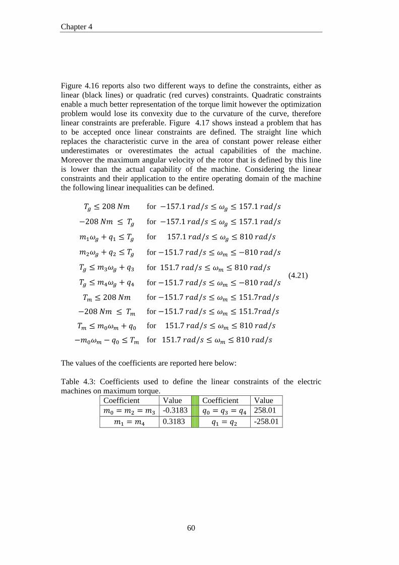
Chapter 4
60
Figure 4.16 reports also two different ways to define the constraints, either as
linear (black lines) or quadratic (red curves) constraints. Quadratic constraints
enable a much better representation of the torque limit however the optimization
problem would lose its convexity due to the curvature of the curve, therefore
linear constraints are preferable. Figure 4.17 shows instead a problem that has
to be accepted once linear constraints are defined. The straight line which
replaces the characteristic curve in the area of constant power release either
underestimates or overestimates the actual capabilities of the machine.
Moreover the maximum angular velocity of the rotor that is defined by this line
is lower than the actual capability of the machine. Considering the linear
constraints and their application to the entire operating domain of the machine
the following linear inequalities can be defined.
for
(4.21)
for
for
for
for
for
for
for
for
for
The values of the coefficients are reported here below:
Table 4.3: Coefficients used to define the linear constraints of the electric
machines on maximum torque.
Coefficient Value Coefficient Value
-0.3183 258.01
0.3183 -258.01
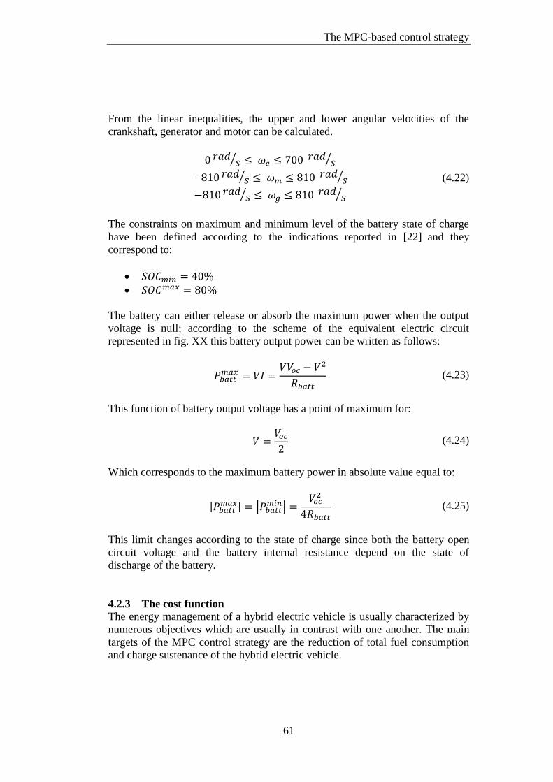
The MPC-based control strategy
61
From the linear inequalities, the upper and lower angular velocities of the
crankshaft, generator and motor can be calculated.
(4.22)
The constraints on maximum and minimum level of the battery state of charge
have been defined according to the indications reported in [22] and they
correspond to:
The battery can either release or absorb the maximum power when the output
voltage is null; according to the scheme of the equivalent electric circuit
represented in fig. XX this battery output power can be written as follows:
(4.23)
This function of battery output voltage has a point of maximum for:
(4.24)
Which corresponds to the maximum battery power in absolute value equal to:
(4.25)
This limit changes according to the state of charge since both the battery open
circuit voltage and the battery internal resistance depend on the state of
discharge of the battery.
4.2.3 The cost function
The energy management of a hybrid electric vehicle is usually characterized by
numerous objectives which are usually in contrast with one another. The main
targets of the MPC control strategy are the reduction of total fuel consumption
and charge sustenance of the hybrid electric vehicle.

Chapter 4
62
Consequently these two performance indices are included in the cost function by
means of two quadratic terms which represent the instantaneous fuel mass flow
rate and the deviation of the battery state of charge with respect to its reference
value. The reference value is 60% and it has been selected according to the
suggestion given in [22]; this value is kept constant throughout the driving
mission for any drive cycle. The cost function includes other terms that stabilize
the control action like the penalty weights on the levels and variations of the
control inputs.
(4.26)
The second power of each term appear in the cost function in order to define a
quadratic objective and thus retain the standard formulation of a quadratic
programming problem.
4.2.4 The linearized state space form
A MPC based control strategy can even exploit a nonlinear reference model to
predict system outputs and calculate an optimal control action. In this case the
approach is called Nonlinear MPC (NLMPC) and it requires generally a high
computational effort and some doubt that a NLMPC can be practically
implemented as control strategy for the energy management [14]. For this reason
a linear time varying model predictive control strategy (LTV-MPC) has been
developed in this thesis. A LTV-MPC follows the standard approach reported in
the reference literature [23] where a discretized linear state space form is used as
reference model to develop an optimal control strategy. From the nonlinear state
space form a linearized state space form is obtained as a truncated Taylor series
around a specific operating condition. At each sampling time the values of the
states, control inputs, measured disturbances are sampled and stored in the
correspondent vectors . The small variations about the linearization
point of these vectors can be approximated through linear functions according to
a Taylor series which is truncated at the linear terms. Then the system is
discretized applying Euler forward with a constant discretization period. The
partial derivatives of the state and output equations are evaluated at the
linearization point and the final outcome is a set of matrices which relates the

The MPC-based control strategy
63
system outputs and the time derivatives of the states to the variations of the
states themselves, the control inputs and the external measured disturbances.
The system can be written in matrix form as follows:
(4.27)
with a further substitution, it can be simplified to:
(4.28)
where:
Euler forward is applied to discretize the linearized state space form. According
to this approach a continuous time derivative evaluated at time t is approximated
by a forward finite difference as follows:
(4.29)

Chapter 4
64
Suppose that the independent variable t can only assume discrete levels with
, then the variation is finite. Consider now that the variation
corresponds to the discretization period , thus the linearized state space form
can be discretized as follows:
(4.30)
By rearranging the terms in (4.30) the following final matrix formulation is
found:
(4.31)
where the pedix d stands for discrete. The matrices which appear in the output
equations are actually equal to those of the continuous linearized state space
form since the discretization only introduces some changes in the discrete time
derivatives of the state equations. The discrete state space form (4.31) represents
the basis of the MPC approach. The approach takes the title “time varying”
since at each sampling time the new available information on system states,
control inputs and measured disturbances are used to compute the new matrices
of the linearized system. In Appendix A it is described how this state space form
is used to predict the sequence of system outputs, to build the matrix form of the
constraints and the matrix form of the cost function in order to set up the
optimization problem. As previously remarked the regression model of the
generator power loss introduces a problem to calculate the partial derivatives
since the angular velocity of the rotor appears with the absolute value. In
practice even the linearized state space form contains still a nonlinear term given
by the derivative of the absolute value of the angular velocity of the rotor of the
generator. In order to solve this issue and retain a linear formulation of the
partial derivatives of the generator power loss, two different expressions of the
matrices of the linearized state space form have been defined. In particular the
sign of the coefficients of the regression model is changed according to the sign
of the generator angular velocity; in this way the components of the matrices
have two possible expressions. The sign of the generator angular velocity is
determined at the sampling time through equations (4.11) and it is assumed that
it does not change over the prediction horizon. Depending on the sign the
following regression model is assumed to calculate the partial derivatives of the
battery power.

The MPC-based control strategy
65
if
if
(4.32)
Important problems related to linearization of the state space form and this latter
approximation are treated afterwards.
4.2.5 Quadratic Programming and Active set method
According to the matrix formulation provided in Appendix A, the optimization
problem is formulated as a Quadratic Programming problem meaning that the
cost function is a quadratic function of the control variables and the constraints
are expressed as linear inequalities in the control variables as well.
Consequently the Quadratic Programming problem which strives to find the
optimal control action can be formulated as follows:
s.t.
(4.33)
where is vector of constant terms which is neglected in the following.
The number of inequality constraints is generally higher than the number of
optimization variables, however these constraints comprise active and inactive
constraints. An inequality constraint is said to be active when the strict equality
holds:
(4.34)
where bi stands for the i-th constraint, Ai is the i-th row of matrix A.
An active constraint influences the optimal solution since the objective function
is forced to move along this constraint, hence if this constraint were removed
from the problem the optimal solution would be different. On the other hand an
inactive constraint does not influence the optimal solution and thus it can be
neglected in the optimization problem. In order to find a solution to problem
(4.33) it is necessary that the number of active constraints is lower than the
number of variables to be optimized. In order to assure the convexity of the
Quadratic Programming problem the matrix H has to be positive definite or at
least semi-positive definite. This property is guaranteed by a proper definition of
the penalty weights in the cost function; in particular, using the same notation as
Appendix A, the matrices which contain the penalty weights on
outputs and on levels and variations of control inputs should be semi-positive
definite. Being H semi-positive definite assures that the cost function is convex
and convexity of the whole optimization problem is guaranteed when the

Chapter 4
66
constraints are linear because they identify flat faces on the convex objective
surface thus the feasible domain of the design variables is still convex [23]. The
optimization problem is solved numerically with a refined active-set method.
Active-set is a primal method, thus it works directly on the given objective and
constraint functions to find an optimal solution. The active set method defines at
each step a group which is supposed to contain the constraints which are active
at a given point . This set is termed working set and the optimization is
limited to the resulting working surface in the feasible domain of the variables to
be optimized. The numeric routine starts by guessing a working set of the
problem and by looking for a feasible optimum inside the working surface
however since the composition of the working set is not known in advance and
any point defined by the algorithm has to be feasible, the algorithm checks at
any new iteration that any other constraint which is outside the working set is
satisfied otherwise it is added to a new working set and the optimization is
repeated. Regarding model predictive control, active set and interior point
methods are applied the most and the issue to determine which algorithm suits
better for MPC applications is still unsolved. In this thesis active set method has
been used since interior point method tends to find an optimum far from the
constraints due to the barrier functions. For this kind of problem it is likely that
the optimal solution lies on the constraints rather than inside the working
surface. Moreover a high efficient algorithm for convex quadratic programming
problem was available [24] and the time required to solve a single optimization
problem was much shorter in comparison to Matlab® built-in functions.
4.3 How the strategy works
The code of the strategy has been implemented in Simulink®
and run in
cosimulation with Amesim®. The high fidelity model of the hybrid powertrain is
implemented in Amesim® thus these two software communicates at each
sampling time. The communication is organised in two steps, in the first part the
control strategy samples the values of the inputs from the Amesim® model and
uses this values to elaborate the optimal control actions. Subsequently the
control inputs are sent to the vehicle model and kept with zero order hold along
the following sampling period. The inputs and outputs of the control strategy
are:
Inputs:
Driver’s torque request at driven wheels
Vehicle longitudinal speed
Battery state of charge
Crankshaft angular velocity
Engine torque
Generator torque
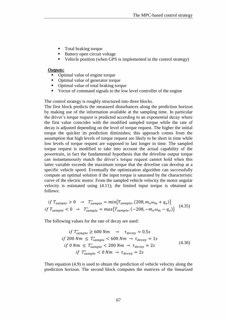
The MPC-based control strategy
67
Total braking torque
Battery open circuit voltage
Vehicle position (when GPS is implemented in the control strategy)
Outputs: Optimal value of engine torque
Optimal value of generator torque
Optimal value of total braking torque
Vector of command signals to the low level controller of the engine
The control strategy is roughly structured into three blocks.
The first block predicts the measured disturbances along the prediction horizon
by making use of the information available at the sampling time. In particular
the driver’s torque request is predicted according to an exponential decay where
the first value coincides with the modified sampled torque while the rate of
decay is adjusted depending on the level of torque request. The higher the initial
torque the quicker its prediction diminishes; this approach comes from the
assumption that high levels of torque request are likely to be short in time while
low levels of torque request are supposed to last longer in time. The sampled
torque request is modified to take into account the actual capability of the
powertrain, in fact the fundamental hypothesis that the driveline output torque
can instantaneously match the driver’s torque request cannot hold when this
latter variable exceeds the maximum torque that the driveline can develop at a
specific vehicle speed. Eventually the optimization algorithm can successfully
compute an optimal solution if the input torque is saturated by the characteristic
curve of the electric motor. From the sampled vehicle velocity the motor angular
velocity is estimated using (4.11); the limited input torque is obtained as
follows:
(4.35)
The following values for the rate of decay are used:
(4.36)
Then equation (4.9) is used to obtain the prediction of vehicle velocity along the
prediction horizon. The second block computes the matrices of the linearized

Chapter 4
68
state space form using the inputs acquired at the sampling time; moreover it uses
the predictions of the external disturbances to compute the matrices which
define the constraints and the cost function. The expressions of these matrices is
reported in Appendix A. Note that the sampling period is different than the
prediction period used to discretize the system, this latter is longer in order to
have a sufficient long prediction horizon with a limited number of variables to
be optimized.
The penalty weights applied to the outputs are assigned according to an
exponential decay along the prediction horizon in order to reduce the influence
of the last samples which are far from the linearization point. The values of
these outputs are predicted using the linearized state space form, hence they are
likely to be not correct and thus not important for the optimization problem. The
values of the penalty weights are assigned as function either of the input power
request or the torque request; the following table is used:
Table 4.4: Penalty weights defined in the cost function.
Input level
0 10 0.1 1 0.1 2 0.01 0.01
0 1 0.1 1 0.1 0 0.01 0.01
0 10 0.01 0.01 0.01 2 0.005 0.005
(**)
1 1.8 4e-4 1e-4 0.001 2 0.005 0.005
(**)
1 1.8 4e-4 1e-4 0.001 2 0.01 0.05
(*)
1 1.8 4e-4 1e-4 0.001 2 0.01 0.05
(*)
1 1.8 3e-4 1e-4 0.001 2 0.01 0.05
1 1.6 1e-4 1e-4 0.001 2 0.01 0.05
Considering the power levels denoted with (**) when either the vehicle velocity
is lower than 4.7 m/s or the battery state of charge is above the reference level, is set equal to 0 while is set equal to 7 or 2 in order to encourage
MPC to exploit electric traction. For power levels denoted with (*) is set
equal to 0 when the battery is overcharged. Moreover every time the vehicle

The MPC-based control strategy
69
velocity is below 0.1 m/s, then is set equal to 10 in order to encourage MPC
to switch off the engine. The penalty weight is set equal to 0.1.
The last block solves the quadratic programming problem using the sequence of
optimal control actions defined at the previous sampling time as initial guess.

Chapter 4
70

5 Results
In this chapter all relevant results are shown and discussed. Firstly the nonlinear
and the linearized state space models are validated, thus some figures are used to
underline the remarkable considerations about modeling then the MPC-based
control strategy is compared to the rule based strategy regarding fuel economy
and drivability. Fuel economy is addressed firstly while velocity tracking error
and passengers on board comfort during engine starting and stopping is treated
afterwards. In the first part of the chapter it is clarified how the comparative
simulations have been carried out, then the most important results are provided.
It is important to understand how MPC can achieve better fuel economy with
respect to the heuristic control strategy. For this purpose the time history of
some important outputs is displayed e.g. engine operating points, power split in
the powertrain, battery state of charge level. The post processing of the results
permits to conclude that the MPC-based strategy performs better extra urban
driving rather than urban driving moreover it uses engine power to provide the
mean power request while battery power is exploited to deal with acceleration
onset and power fluctuations. A simplified analysis of on board passengers
comfort is then shown following the specifications provided in [25]. Engine
starting and engine stopping have been considered as the input events for
comfort evaluation.
5.1 Validation of the models
The nonlinear and the linearized state space forms have been validated by
assigning the time history of the control inputs and external disturbances and
comparing the outputs with those obtained in Amesim® for the same drive cycle.
The trends of the inputs have been obtained by a reference simulation on NEDC
that has been run in Amesim® using the rule based strategy. The nonlinear state
space form has been integrated using Euler forward with a fixed integration
period of 1ms. The nonlinear model provides an acceptable description of the
dynamics of the battery state of charge and of the angular velocity of the
crankshaft as the next two figure illustrate. The nonlinear model can therefore
capture the most important events of the system even if the compliances of the
vehicle are not taken into account.
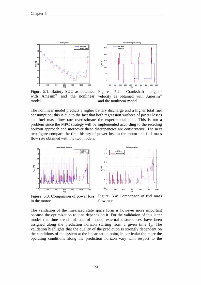
Chapter 5
72
Figure 5.1: Battery SOC as obtained
with Amesim® and the nonlinear
model.
Figure 5.2: Crankshaft angular
velocity as obtained with Amesim®
and the nonlinear model.
The nonlinear model predicts a higher battery discharge and a higher total fuel
consumption; this is due to the fact that both regression surfaces of power losses
and fuel mass flow rate overestimate the experimental data. This is not a
problem since the MPC strategy will be implemented according to the receding
horizon approach and moreover these discrepancies are conservative. The next
two figure compare the time history of power loss in the motor and fuel mass
flow rate obtained with the two models.
Figure 5.3: Comparison of power loss
in the motor.
Figure 5.4: Comparison of fuel mass
flow rate.
The validation of the linearized state space form is however more important
because the optimization routine depends on it. For the validation of this latter
model the time trends of control inputs, external disturbances have been
assigned along the prediction horizon starting from a given time . The
validation highlights that the quality of the prediction is strongly dependent on
the conditions of the system at the linearization point, in particular the more the
operating conditions along the prediction horizon vary with respect to the
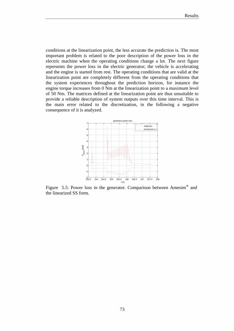
Results
73
conditions at the linearization point, the less accurate the prediction is. The most
important problem is related to the poor description of the power loss in the
electric machine when the operating conditions change a lot. The next figure
represents the power loss in the electric generator; the vehicle is accelerating
and the engine is started from rest. The operating conditions that are valid at the
linearization point are completely different from the operating conditions that
the system experiences throughout the prediction horizon, for instance the
engine torque increases from 0 Nm at the linearization point to a maximum level
of 50 Nm. The matrices defined at the linearization point are thus unsuitable to
provide a reliable description of system outputs over this time interval. This is
the main error related to the discretization, in the following a negative
consequence of it is analyzed.
Figure 5.5: Power loss in the generator. Comparison between Amesim
® and
the linearized SS form.
253.5 254 254.5 255 255.5 256 256.5 257 257.5 258-2
-1
0
1
2
3
4
5
6
7generator power loss
t [s]
Pglo
sS [
kW
]
AMESim
linearized ss
Chapter 5
74
5.2 Fuel economy
5.2.1 Drive cycles and charge sustenance
Fuel consumption of a vehicle depends on both road conditions (e.g. road slope,
wind velocity) and vehicle parameters (e.g. total mass, coefficient of
aerodynamic resistance). In order to provide a ranking of different vehicles
regarding fuel economy performance which is independent on road conditions,
standardized drive cycles have been developed for the sake of testing different
vehicles under the same driving conditions. A drive cycle defines the reference
velocity and road slope profiles that the vehicle will follow during a specific
driving mission. The absolute wind velocity is usually set equal to 0 m/s and the
gear shifting schedule is also specified for those vehicles equipped with a
manual transmission. The United States, Europe and Japan have correspondent
standardized drive cycles which strive to replicate urban and extra-urban driving
conditions. The characteristics of these cycles are regularly updated in order to
match the actual performance of vehicles on the market. Anyway each cycle
underestimates the real road load that a vehicle would encounter in actual
driving and therefore they should be used merely as a basis for direct
comparison among different vehicles rather than as a way to predict fuel
consumption. Five reference drive cycles have been used in this thesis work to
compare the achievable fuel economy between a rule based strategy and the
MPC-based control strategy. In appendix C the reference velocity profile of
these cycles is provided. The results that are reported here refer to a flat road
otherwise specified. The hybrid electric vehicle that is analyzed is of charge
sustaining type as a consequence a correct evaluation of fuel economy over a
specific drive cycle can be done provided that energetic equilibrium is achieved,
namely the battery state of charge level at the end of the simulation equates the
initial value. This equal level is called state of charge equilibrium level in the
following. In order to achieve this condition the same cycle has been repeated
several times until energetic equilibrium has been obtained.
Amesim® provides as output the total mass of the fuel in grams that has been
burnt during the driving mission; from this output result it is possible to
calculate the fuel economy according to the following equations and by
assuming a fuel density equal to .
(5.1)

Results
75
(5.2)
5.2.2 Comparison of the results
The following table and the following histogram summarize the total fuel
consumption and equilibrium level of the battery state of charge as obtained
when the two control strategies are applied to the 5 reference drive cycles.
Table 5.1: Comparison of fuel economy. Final results. Rule based MPC
Cycle
NEDC 59.86 509.03 5.927 59.49 493.6 5.742
HWFET 59.65 751.25 5.837 59.73 741.62 5.762
SC03 47.97 286.47 6.378 57.34 261.16 5.815
UDDS 58.14 546.0 5.840 57.46 541.59 5.793
US06 42.00 901.59 8.973 56.17 741.53 7.380
Figure 5.6: Percentage reduction of fuel consumption given by MPC with
respect to the rule based strategy.
Table 5.1 reports the fuel economy in absolute value while the histogram in
Figure 5.6 reports the fuel economy achievable with MPC in terms of
percentage reduction with respect to the baseline represented by the rule based
strategy.

Chapter 5
76
The MPC-based energy management strategy succeeds in reducing fuel
consumption over all standard driving cycles with respect to the rule based
strategy. Charge sustainability is achieved by both strategies. Regarding the
battery state of charge level it is important that it never exceeds the minimum
and maximum thresholds imposed by the operating constraints and its
equilibrium level should be reasonably close to the reference one. From the table
it is possible to see that the proposed optimal control strategy can keep the
equilibrium level close to the reference value (60%) and in some situations
(US06, SC03) it performs better than the rule based strategy. The next figures
illustrate the time history of the battery state of charge level as obtained over the
five reference drive cycles. It can be concluded that the MPC-based control
strategy manages to maintain the battery state of charge level within the
operating constraints; on the opposite the rule based strategy violates the
minimum threshold in US06. It is stressed here that the heuristic control strategy
samples the input information at each simulation step while the MPC-based
strategy samples with a fixed sampling period. This is a remarkable piece of
advantage for the rule based strategy because the control inputs are updated at
each simulation step.

Results
77
a) b)
c) d)
Figure 5.7: Comparison of battery state of charge level over the 5 considered
drive cycles as obtained with the rule based strategy (blue curves) and the MPC-
based strategy (red curves). a) top left NEDC, b) top right HWFET, c) mid left
SC03, d) mid right UDDS, e) low US06
The results are nice however it is clear that the improvement brought by MPC in
terms of fuel consumption reduction is sensitive to the driving conditions

Chapter 5
78
specified by a drive cycle. In fact MPC performs much better than the heuristic
control strategy over SC03 and US06 while the performance is comparable over
NEDC and UDDS. This conclusion is linked to the different operating principles
of the two strategies consequently it is worth to analyze them in details. Firstly
the MPC-based energy management strategy is analyzed on its own to highlight
its main operating principle then it is compared against the rule based strategy.
5.2.3 The operating principles of the two control strategies
The European drive cycle NEDC is the basis to illustrate the basic operating
principle of the optimal control strategy since the urban part of this cycle
involves the repetition of a basic velocity profile four times and hence
comparisons can be made between two repetitions. The next figure reports the
velocity profile of the portion of the cycle that is used here to analyze the
operating principle of the MPC strategy.
Figure 5.8: Velocity profile of the driving situation used to analyze the
operating principle of the MPC strategy.
This portion of the cycle involves a rather long acceleration followed by a pretty
short phase of constant vehicle speed; then a long braking brings the vehicle to
complete stop. The power flow among the powertrain components that
corresponds to this driving situation is represented in the following figure.

Results
79
Figure 5.9: Correspondent power flow in the powertrain.
This portion of the cycle highlights how MPC exploits all available driving
modes, for instance it employs firstly full electric driving from 50s to almost 57s
when vehicle speed is low and during the initial part of the acceleration. Once
power request increases more the engine is activated. The generator is used as
engine starter and the battery provides additional power to start the engine. The
final part of the acceleration is supported by the engine and the battery together;
this is the positive split mode since part of the engine power is sent to the motor
through the electric side of the powertrain. From 61s to 85s the vehicle is
cruising at low speed and power request reduces significantly. Initially the
electric mode is still exploited and the engine runs in idle, however as the
battery state of charge diminishes the engine torque is increased once more and
positive split mode is used to run the vehicle and charge the battery
simultaneously. Contrary to the previous case the portion of the engine power
that is sent to the electric side of the powertrain is fully used to charge the
battery. In this situation the engine provides the whole traction power. At 85s
regenerative braking is applied to recover the vehicle’s kinetic energy; however
part of the upstream flowing power cannot can be stored in the battery due to
power loss. At 90s the generator torque is used to stop the engine.
The same velocity profile is followed between 240s and 300s but the battery
state of charge is lower in this second case, thus MPC uses a higher engine
torque to reduce the load on the battery and maintain the state of charge level
reasonably close to its reference value. This behavior is displayed in the next
group of figures which report a direct comparison of the engine torque level
decided by MPC and the correspondent battery state of charge level.

Chapter 5
80
Figure 5.10: Battery state of charge and engine torque for two repetitions of the
same velocity profile.
The trend of the engine torque is the same except for the magnitude of the
torque which is adjusted in order to provide more power to the electric side of
the powertrain. It is important to note that MPC prefers increasing the engine
torque rather than the crankshaft angular velocity in order to provide more
power to the battery. This solution allows the engine to operate in a region of
low fuel consumption. MPC exploits steadily the power split between the engine
and the battery where the split ratio depends on the driving situation and on the
instantaneous battery state of charge level. The result is a smooth activation of
the engine during hard accelerations and a less fluctuating engine operating
point during all other driving situations. Moreover MPC takes advantage of
regenerative braking to charge the battery and reduce the future power load to
the engine; simultaneously the engine torque is quickly reduced to 0 Nm as soon
as braking is detected.
The rule based strategy uses the engine as primary power unit either when the
power request is high i.e. during acceleration phases, or when the battery state of
charge is close to its minimum threshold. Engine power is used to follow the
peaks in power request so this control strategy adjusts the engine operating point
in accordance to the input level of power request. This behavior has the
drawback that the engine is activated brutally as the battery state of charge
diminishes below a threshold level or power request exceeds a limit value. The
engine operating point moves quickly towards a region in the engine map where
high power is generated in order to drive the vehicle and charge the battery.

Results
81
In order to illustrate the differences in the operating principles of the two
strategies, a portion of the urban part of the European drive cycle (NEDC) is
used as reference. This driving situation includes a sequence of accelerations
followed by a short time interval where vehicle speed is constant as reported in
the next figure.
Figure 5.11: Velocity profile which corresponds to the considered driving
situation.
The following two figures report the correspondent power flow among the
components of the powertrain that is obtained by the application of the two
energy management strategies.
Figure 5.12: Power flow in the powertrain as obtained with the rule based strategy
(left)and with MPC (right).
The rule based strategy uses the engine power to balance the highest power
request during the acceleration phase; in this situation the crankshaft rotates
quicker than the ring gear (if their velocities are referred to the same shaft) and
therefore positive split mode is employed. Between 720s and 730s the power

Chapter 5
82
released by the battery is almost null; the electric power produced by the
generator is sent to the electric motor but eventually this implies that the fuel is
the only energy source in this situation. Positive split mode is also applied by
MPC which already activates the engine between 712s and 720s; however the
battery power is used much more to sustain the load during acceleration in
comparison to the rule based strategy. This implies that more engine power has
to be used to replenish the battery state of charge level during the subsequent
phase where the vehicle is cruising between 730s and 740s. Nonetheless the
total load is low in this second driving condition therefore the engine can release
a surplus of power to charge the battery while still operating in a region of high
efficiency. The following figures report the engine operating points on the
engine map which result from the decisions taken by the two energy
management control strategies.
Figure 5.13: Engine operating points as obtained with the rule based strategy (left) and
with MPC (right).
MPC can successfully keep the fuel mass flow rate low in comparison to the
heuristic control strategy however the engine is used longer in time than with the
rule based control strategy and eventually the benefit is negligible over the
urban portion of the cycle. In fact if just the urban portion of NEDC were used
as a new driving mission the fuel economy obtainable with the two strategies
would be the same.
Table 5.2: Fuel economy and battery state of charge equilibrium level over the urban
portion of NEDC. Driving mission limited to the urban portion of NEDC
Strategy
Rule based 50.48 % 5.601
MPC 58.42 % 5.613
UDDS is another urban cycle which includes frequent start and stop of the
vehicle and the average speed is below 10 m/s, hence the average power request

Results
83
is low. Even in this case the fuel economy achievable with MPC is slightly
better than the rule based strategy as it is reported in Table 5.1.
On the other hand when power request increases MPC achieves better results.
Considering the following part of the highway cycle (HWFET) where the
vehicle accelerates in the initial part then speed remains almost constant.
Figure 5.14: Velocity profile of the considered portion of HWFET.
The power flow in the powertrain as obtained with the two strategies is reported
in the next two figures.
Figure 5.15: Power flow with the rule
based strategy in HWFET.
Figure 5.16: Power flow with MPC in
HWFET.
MPC manages the engine power in order to provide the mean power request
while battery power is used to deal with power fluctuations, thus the battery
provides an energy buffer to maintain the engine operating point close to a value
of high efficiency.

Chapter 5
84
On the opposite the rule based strategy strives to continuously update the engine
operating point to the actual power request. From this point of view this latter
strategy does not take advantage of the additional mechanical degree of freedom
given by the power-split drive which enables to decouple the engine operating
point from the vehicle speed. In fact from Figure 5.15 it can be seen that battery
power is kept around the null value, this proves that the rule based strategy
mainly uses the engine power to match the input power request. Figure 5.16
shows instead how MPC splits the total power request between the engine and
the battery whose power oscillates a lot to deal with fluctuations of power
request. This operating principle of MPC comes from the definition of the cost
function which penalizes instantaneously the fuel mass flow rate and the
deviation of the state of charge. The next two figures represent the engine
operating points as defined by the two control strategies.
Figure 5.17: Engine operating points
defined by the rule based strategy.
Figure 5.18: Engine operating points
obtained with MPC.
The rule based strategy sets the desired engine operating point at high engine
speed meaning that although the desired operating point falls on the engine
OOL, the fuel mass flow rate is low. On the opposite MPC succeeds in keeping
the engine speed low and thus the fuel mass flow rate is always lower than 1.9
g/s. Thanks to the fact that the engine provides only the mean power request,
MPC can achieve better engine efficiency than the rule based strategy over this
driving situation as the next figure shows; moreover the engine keeps the same
operating principle and the efficiency is almost constant.
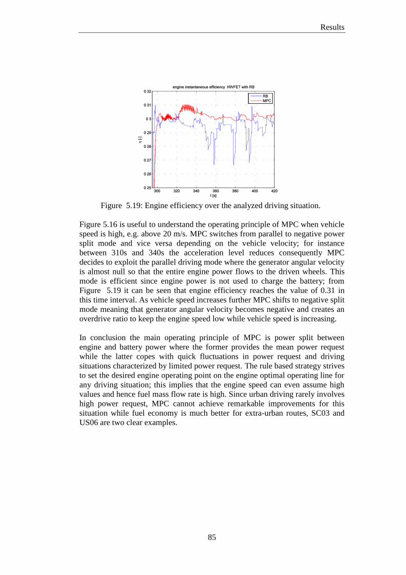
Results
85
Figure 5.19: Engine efficiency over the analyzed driving situation.
Figure 5.16 is useful to understand the operating principle of MPC when vehicle
speed is high, e.g. above 20 m/s. MPC switches from parallel to negative power
split mode and vice versa depending on the vehicle velocity; for instance
between 310s and 340s the acceleration level reduces consequently MPC
decides to exploit the parallel driving mode where the generator angular velocity
is almost null so that the entire engine power flows to the driven wheels. This
mode is efficient since engine power is not used to charge the battery; from
Figure 5.19 it can be seen that engine efficiency reaches the value of 0.31 in
this time interval. As vehicle speed increases further MPC shifts to negative split
mode meaning that generator angular velocity becomes negative and creates an
overdrive ratio to keep the engine speed low while vehicle speed is increasing.
In conclusion the main operating principle of MPC is power split between
engine and battery power where the former provides the mean power request
while the latter copes with quick fluctuations in power request and driving
situations characterized by limited power request. The rule based strategy strives
to set the desired engine operating point on the engine optimal operating line for
any driving situation; this implies that the engine speed can even assume high
values and hence fuel mass flow rate is high. Since urban driving rarely involves
high power request, MPC cannot achieve remarkable improvements for this
situation while fuel economy is much better for extra-urban routes, SC03 and
US06 are two clear examples.

Chapter 5
86
5.2.4 A problem related to linearization
Figure 5.16 and Figure 5.19 show how some high frequency fluctuations appear
when the MPC-based control strategy is used between 300s and 340s; in general
these fluctuations occur every time parallel driving mode is selected. The reason
of this strange behavior is due to the linearization of the generator power loss. In
fact as it was illustrated in chapter 4 in order to linearize the power loss
associated to the generator it is necessary to consider two different formulations
of the partial derivatives of this function with respect to system states, control
inputs and measured disturbances depending on the sign of the generator angular
velocity at the sampling time. However this can generate unrealistic negative
values of power loss associated to electric machines. The next figure reports the
generator angular velocity over the same driving condition; it reveals that MPC
has few problems as soon as this variable gets closer to the null value.
Figure 5.20: Generator angular velocity during parallel driving mode in
HWFET.
This issue cannot be completely solved but it can be attenuated using a penalty
weight on the deviation of the angular velocity of the generator with respect to a
fictitious value in the cost function. This is the reason to include term appears
inside the cost function (4.26). When the vehicle is run in parallel driving mode
the generator angular velocity should be equal to 0 rad/s therefore a fictitious
reference value of 0.1 rad/s is specified in the cost function and MPC is pushed
to adjust the generator torque in order to limit the deviation of the generator
angular velocity from this reference value. The reference value is fictitious since
it is only used to avoid this latter variable from crossing repeatedly the null
value and thus creating uncertainty in the optimal control action due to the fact
that the operating conditions change a lot from one sampling to the following
one.

Results
87
The penalty weight on this deviation is limited in order to allow MPC to change
quickly the driving mode. If this deviation were penalized severely then MPC
would be encouraged to keep the parallel driving mode even when it is not the
most efficient one. The following figures represent this latter point where the
reference on the angular velocity of the generator is introduced in the cost
function and the penalty weight is set rather high (20).
Figure 5.21: Generator angular
velocity once its reference value is
included in the cost function.
Figure 5.22: Power flow in the
powertrain once the reference value of
generator angular velocity is
introduced.
It can be seen that fluctuations have disappeared nonetheless MPC maintains the
parallel driving mode even after 340s. This means that the engine speed is
higher than in Figure 5.16 and thus the fuel mass flow rate is slightly higher too.

Chapter 5
88
5.3 Drivability
5.3.1 Velocity tracking error
A energy management control strategy should satisfy the requests coming from
the driver in particular the reference velocity profile should be tracked correctly.
For each strategy and for each drive cycle the instantaneous error has been
calculated and the resulting mean error and standard deviation are reported in
the following table.
Table 5.3: Velocity tracking error. Mean value and standard deviation.
Rule based MPC
Cycle
NEDC 0.0016 0.0192 0.0016 0.0296
HWFET 0.0022 0.0201 0.0022 0.0226
SC03 0.0028 0.2669 0.0026 0.206
UDDS 0.0013 0.0237 0.0013 0.0376
US06 0.001 1.302 0.0006 1.0029
The tracking error has a slightly higher standard deviation with MPC since both
the control strategy and the low level controller of the electric machines are
implemented as discrete time controllers and hence there is a delay between the
driver’s request and the actual torque produced at the driven wheels. On the
other hand the controllers of the rule based strategy update the control actions at
each sampling time so it can immediately match the driver’s torque request.
5.3.2 Passengers discomfort related to engine starting and stopping
The angular velocity of the crankshaft is controlled by the generator torque.
Once the vehicle supervisory controller decides to activate or to switch off the
engine, the generator torque level is changed rapidly in order to achieve as quick
as possible the new desired set point of the crankshaft angular velocity.
However it is important to verify that the change in generator torque does not
produce undesired oscillations along the driveline which eventually affects
passengers comfort and quality perception of the vehicle. The readiness in the
response of the generator torque can be tuned with the proportional gain of the
PI control on the instantaneous error between current and desired crankshaft
angular velocity. This PI feedback control is implemented in the low level
controller of the electric machines. In the next figures the results obtained with
the rule based strategy over NEDC are displayed when the proportional gain of
the low level controller of the electric machines is set equal to 1. The same
driving situation considered in Figure 5.8 is analyzed and the correspondent
carbody accelerations and jerks along the longitudinal and the vertical axes are
plotted.

Results
89
Figure 5.23: Carbody accelerations
during engine starting.
Figure 5.24: Carbody jerks during
engine starting.
Engine is activated at 58.5s and this event is clearly recognizable in the
oscillations of the carbody accelerations and jerks. It is impossible to give an
objective evaluation of discomfort, anyway it is necessary to reduce the effect of
these oscillations on passengers comfort. In [26] it is claimed that a magnitude
of jerk above should be avoided while [25] provides an engineering
tool to evaluate the effect of vibrations on people even if the equations provided
in the standard norm refer to continuous vibrations and not transient events like
engine starting and stopping.As these figures show, the variations in carbody
longitudinal and vertical accelerations are severe when the crankshaft starts
rotating. Both longitudinal and vertical carbody jerks are outside the threshold
of as a result the decisions taken by the energy management strategy
are likely to degrade the on board comfort.
The solution that is implemented by the rule based strategy provides for
reducing the proportional gain of the low level controller of the electric
machines to 0.1. The change is therefore applied outside the strategy itself.
The improvement is remarkable as the next figures show.

Chapter 5
90
Figure 5.25: Carbody accelerations
with a lower proportional gain.
Figure 5.26: Carbody jerks with a
lower proportional gain.
At 61s the longitudinal accelerations still varies consistently but this is related to
the fact that the vehicle stops accelerating and enters a part of constant speed.
The resulting oscillations from the quick drop in torque which occurs at 61s are
not an issue in this case since both drivers and passengers expect to feel them.
Regarding the engine starting, this event is no more clearly recognizable in the
carbody accelerations thanks to a smoother action of the generator torque. The
next two figures compare the generator torque action with a proportional gain
equal to 1 and a proportional gain equal to 0.1.
Figure 5.27: Generator torque for a
unitary proportional gain.
Figure 5.28: Generator torque for a
proportional gain equal to 0.1.

Results
91
Comfort analysis with MPC
The MPC-based control strategy has been developed in order to address the
problem of drastic generator torque variation inside the control strategy itself.
Since the generator torque appears among the control input variables and the
crankshaft angular velocity is a state of the system, then it is possible to limit the
generator torque during engine starting and stopping in order to reach a smooth
response of crankshaft angular velocity. The quality of the solution proposed has
been evaluated according to the criteria suggested in [25] although they refer to
continuous oscillatory events. The purpose is to attenuate the vibrations, not to
solve completely the problem which usually involves different methods like
small changes in combustion process, stiffness of engine mounts; some further
details can be found in [3]. The cycle NEDC is used as reference driving
mission because it involves numerous engine start&stop events which are well
separated from one another and therefore can be distinguished easily. Variation
of motor output torque can also produce remarkable peaks in longitudinal
acceleration and jerk however this torque follows the torque requested by the
driver as a consequence the driver and the passengers would expect such a
variation in torque and the resulting peak acceleration. Furthermore one of the
constraints imposed by the drivability refers to the satisfaction at each instant in
time of the total torque at wheels requested by the driver. As a result the analysis
has been focused on engine starting and stopping events in order to tune the
action of the generator torque and reduce the resulting oscillations.
In order to apply the evaluation method proposed in [25] the longitudinal,
vertical and pitch accelerations of the carbody are used. Only the part of the
acceleration signals which refer to an engine event have been considered, thus
the effect of motor torque and engine events on the carbody accelerations should
be distinguished. In NEDC the engine start&stop events can be easily identified
and decoupled from the variation of motor torque because the engine is
activated or stopped when the vehicle is being driven with constant acceleration
or deceleration thus the motor torque is almost constant. It also means that the
longitudinal acceleration of the vehicle has either a positive or a negative mean
value and the oscillations produced by the engine event builds upon this mean
value. For this reason the mean value of the longitudinal acceleration is not
removed because the passengers’ perception of discomfort is related to the
overall acceleration value. A set of data is extracted for each acceleration signal
in order to consider just the values which correspond to an engine event. The
data are sampled using a rectangular-shaped window which does not introduce
any signal distortion moreover the time period for this analysis is chosen in such
a way that the oscillations damp out significantly so initial and final level of
accelerations are similar and the error due to repetition of the measured signal to
create a periodic one is limited.

Chapter 5
92
The sampling frequency is chosen equal to 1000HZ. This value respects a
constraint given by the norm which prescribes to use a sampling frequency at
least equal to:
where represents a characteristic frequency of the frequency weighting
functions provided by the standard ISO norm. It is assumed that all acceleration
signals are measured at the driver’s seat and the weighting functions
are used to weigh the longitudinal, vertical and pitch acceleration respectively.
The norm prescribes to weigh the signals in the time domain using proper digital
filters having the characteristics defined by the frequency weighting functions.
This operation is carried out by applying recursively a Butterworth digital filter
to an acceleration signal, which is divided into bands of octave, and then by
applying the weight factor defined by the weighting function for that frequency
band. Secondly the signal is reconstructed in time domain by using an inverse
Fourier transform. The weighted signal is used to calculate the weighted
rms value as follows:
(5.3)
The three rms values are combined through the comfort factors ki, which are
provided by the norm, to get the overall equivalent acceleration signal
(5.4)
This value is eventually compared to a reference table provided by the norm
which describes how a normal human being would judge a certain acceleration
level. In order to avoid a feeling of discomfort, the overall equivalent
acceleration should be kept below . These equations hold provided
that the crest factor of the weighted acceleration signal is below 9; for this
reason this value has always been calculated as follows.
(5.5)
If some peaks are present in the signal the following ratio can become useful.

Results
93
(5.6)
T is the observation period of the signal while VDV is called vibration dose
value and it is calculated as follows:
(5.7)
If the ratio (5.6) exceeds 1.75, the norm suggests that the VDV describes better
the acceleration signal rather than its rms value. However if no peaks are present
in the signal and the signal has a mean value which is not null, then the
information given by the VDV is not important because it tends to assume high
magnitude due to the fourth power of the average value. For this reason if an
acceleration signal has no peak, its rms value is assumed to be reliable to
provide a good description even if the above mentioned ratio exceeds 1.75.
The NEDC comprises in total 18 engine events, with 9 starting and 9 stopping
events. An example of calculation is reported afterwards on the basis of the two
first engine events in the cycle NEDC, a starting at 56s and a stopping at 90s.
Firstly consider the engine starting event which is depicted in the following
figure.
Figure 5.29: Carbody accelerations due to engine starting obtained with MPC.
The trend of crankshaft angular velocity with time is similar to that reported in
Figure 5.25 and obtained by the rule based strategy in collaboration with the

Chapter 5
94
low level controller of the electric machines. This is because the generator
torque is applied gradually by the vehicle supervisory controller in order to
achieve the desired set point of the crankshaft angular velocity without
remarkable oscillations of the carbody.
Figure 5.30: Generator torque defined by MPC to start the engine.
Comparing this latter figure to Figure 5.28 it emerges that it takes MPC slightly
longer time to bring the engine to the reference idle speed, thus to activate the
engine. The trends of longitudinal and vertical accelerations are rather smooth
while pitch acceleration shows larger oscillations which however are already
present when the engine is started. The three considered acceleration signals are
reported below once more together with the results obtained by applying
equations (5.3) to (5.4).
Figure 5.31:Longitudinal
acceleration
Figure 5.32: Vertical
acceleration.
Figure 5.33: Pitch
acceleration.

Results
95
The equivalent total acceleration is equal to:
The ratio defined in (5.6) is bigger than 1.75 for the longitudinal acceleration
signal which however does not show any spike, thus the high value of the VDV
is due to the mean value of this signal. The crest factor of the weighted
acceleration signal is far from 9 as a result the VDV value is not used to
describe the discomfort felt by the passenger.
At 85s the driver starts braking and the electric motor torque switches quickly to
negative values to accomplish a regenerative braking. The engine torque drops
rapidly to 0 Nm and this produces a small variation on the crankshaft angular
velocity which goes below the idle speed for a while, then MPC decides to use
the generator torque to bring the flywheel angular velocity back to the idle
speed. The oscillations in the acceleration signals produced by engine stopping
can be recognized easily since motor torque remains almost constant in this
phase(5)
. The next figure represents these output variables.
5 The variation of generator torque affects the motor torque too because a negative generator
torque is needed to slow down the crankshaft rotation and this corresponds to a positive torque
applied to the driveline output shaft. Consequently in order to satisfy the equilibrium equation
and produce the same output torque, the motor should produce a higher negative torque. All
these events are related to engine stopping as a result they are treated all together.

Chapter 5
96
Figure 5.34: Carbody accelerations during engine stopping.
The following results are obtained:
The results computed for the other 16 events are reported in the next table.
Table 5.4: Equivalent accelerations related to engine start&stop events.
starting stopping
0.4941
All values are below .
6 Additional analyses
In this chapter some additional investigations on the performance of the MPC-
based control strategy are presented. In the following the terms internal and
external parameters are used extensively and the chapter is divided into two
main parts where each focuses on one of these two cases. The term external
parameters refers to all model parameters which lie outside the strategy itself
and contribute to define the vehicle properties. These parameters cannot be
tuned by the controller whereas they are imposed by the driving conditions or by
the design of the vehicle. On the opposite the internal parameters appear in the
script of the strategy and contribute to manipulate the optimization problem,
thus they influence the optimal control action defined by MPC. The scope of
these further analyses is to assess the robustness of the control strategy against
uncertainty of some external parameters of the model and the influence of the
internal parameters on the optimization problem. In the latter case the target is to
identify a set inside the input space of the internal parameters which allows the
energy management control strategy to achieve the best fuel economy. The
possibility to flank the optimal control strategy with additional information
coming from navigation systems like GPS has also been tested in the latest part
of the chapter. The analyses reported in this chapter permits to judge the most
important features of the proposed optimal control strategy.
6.1 Robustness of the control strategy
The optimal values of the control inputs are determined as solutions of a
constrained optimization problem and the reference state space form changes at
each sampling time since it is linearized around the new operating conditions.
Consequently it is not possible to assess stability and robustness of the control
strategy towards parameters uncertainty using the mathematical approach of
classic control theory. This point is actually very important since some vehicle
parameters appear inside the control strategy hence their uncertainty may affect
negatively the performance of the strategy. The typical approach is to test the
behavior of the strategy against a number of different scenario which involve
changing the level of some of the model parameters. As a result some numerical
simulations have been run in order to evaluate the behavior of the strategy with
respect to the variability of some vehicle parameters. Different driving scenarios
have been considered where the value of one parameter at a time has been
modified with respect to a base case. The stability of the strategy has been
evaluated according to these two principles:

Chapter 6
98
The time history of control variables as defined by the control strategy
do not show unrealistic trends, namely they do not oscillate heavily or
quickly switch to a new set point
The battery state of charge remains within the desired operating band
(40% - 80%) and the equilibrium level is reasonably close to the
reference value (60%)
Instead the robustness has been evaluated by means of a comparison with the
results obtained by the rule based strategy for the same driving conditions. The
comparisons have compared the total fuel consumption and the equilibrium
level of the battery state of charge achievable with the two strategies. The results
that are displayed afterwards refer to a system in energetic equilibrium.
The vehicle model in Amesim® contains several parameters but just a set of
them is supposed to have an important influence on fuel economy. In particular
the following parameters have been taken into account:
Carbody mass
Road slope
Dimensionless coefficient of aerodynamic drag
Wheels rotary inertia
Stiffness of the silent chain in the transaxle
Adhesion coefficient between tyre and asphalt
The simulations have been carried out according to the one-at-a-time principle
(OAT) where the level of one factor is modified at a time while all other factors
are kept equal to their base value. The NEDC has been used as reference driving
mission since it comprises pieces of both low power and high power request.
6.1.1 Carbody mass
The carbody mass corresponds to the total vehicle mass minus the front and rear
unsprung masses. This variable changes in accordance with the number of
people on board and the mass of the luggage. The base value is equal to 1280
kg; the following four levels have been tested:
1100 kg, 1400 kg, 1550 kg, 1700 kg
The value 1100 kg is only used to widen the domain of analysis but it is not a
realistic condition since the base case corresponds to a situation with a nominal
vehicle plus the driver. The following figures and tables compare the rule based
strategy to the MPC control strategy in terms of the effect of parameter change
on fuel consumption with respect to the base case.

Additional analyses
99
Figure 6.1: Battery SOC equilibrium
level as function of carbody mass
change.
Figure 6.2: Total fuel consumption as
function of carbody mass change.
Table 6.1: Performance of the two strategies against carbody mass variation.
rule
based 57.88 % 59.86 % 60.61 % 61.36 % 61.83 %
MPC 59.38 % 59.49 % 59.69 % 59.74 % 59.75 %
rule
based 466.7 g 509.0 g 537.9 g 574.9 g 612.5 g
MPC 454.6 g 493.6 518.4 g 549.7 g 581.4 g
Carbody
mass 1100 kg 1280 kg 1400 kg 1550 kg 1700 kg
Increasing the carbody mass leads to an increase of the equilibrium level of the
battery state of charge because during regenerative braking more energy
associated to the inertia of the vehicle can be recovered. Since the strategies
strive to maintain the battery state of charge close to its reference value this
produces eventually a higher equilibrium level because the strategies do not
know that a long braking concludes the cycle. Similarly more power is required
to accelerate the vehicle consequently the total fuel consumption increases too.
The percentage variation of fuel economy with respect to the base case is
reported in the next table.

Chapter 6
100
Table 6.2: Fuel economy percentage variation with respect to carbody mass.
rule based 5.434 5.927 6.263 6.694 7.132
-8.31 % 0.0 % +5.67 % +12.94 % +20.33 %
MPC 5.293 5.742 6.036 6.400 6.770
-7.82 % 0.0 % +5.12 % +11.46 % +17.90 %
carbody
mass 1100 kg 1280 kg 1400 kg 1550 kg 1700 kg
The MPC-based energy management strategy performs better than the rule
based strategy in terms of percentage increase of total fuel consumption. Both
strategies manage to keep the battery state of charge level in-between the
desired operating domain. The MPC-based control strategy seems to be stable as
the next figure shows. This figure represents the time history of the engine
power in the high speed part of NEDC as function of the base value and higher
values of the carbody mass.
Figure 6.3: Engine power as function of carbody mass levels.
The trends are similar, the magnitude of power release is adjusted according to
the increase in carbody mass and the behavior is stable. The next two figures
also serve to highlight that MPC only adjust the engine torque and engine
angular velocity in order to produce more or less power but the operations of the
engine are not modified. This indicates a recurring behavior of MPC despite the
change in operating conditions; hence the strategy is stable and robust.

Additional analyses
101
Figure 6.4: Engine torque as function
of carbody mass.
Figure 6.5: Engine speed as function
of carbody mass.
6.1.2 Road slope
The road surface has been defined as an inclined plane with constant slope,
hence the vehicle moves forward on a road of linear increasing height. However
the initial and the final part of the road are flat. The road profile is therefore
simple but this approach allows fuel economy to be directly related to a specific
road slope. The reference velocity profile has not been modified according to the
change in road slope, thus the driver still tries to follow the velocity profile
which holds for a flat road. This assumption implies that power request
increases significantly in the high speed part of the cycle therefore rather limited
slope values have been tested. The base case corresponds to a null road slope
value; the following conditions have been considered:
The next figure illustrates the road height as function of vehicle position in the
absolute frame for the case of 0.6°.

Chapter 6
102
Figure 6.6: Road height as function of vehicle absolute position. Road slope is
equal to 0.6° and the absolute position of carbody center of gravity is 3422.85
m.
The following results have been obtained.
Figure 6.7: SOC equilibrium level as
function of road slope.
Figure 6.8: Fuel consumption as
function of road slope.
Table 6.3: Values of the results displayed in the two figures above. rule
based 59.86 % 59.44 % 58.86 % 56.99 % 50.75 %
MPC 59.60 % 58.78 % 57.88 % 56.53 % 52.53 %
rule
based 509.0 g 559.0 g 611.2 g 685.4 g 886.2 g
MPC 493.6 g 538.8 g 583.5 g 651.5 g 843.6 g
road
slope 0° 0.3 ° 0.6 ° 1 ° 2 °

Additional analyses
103
Table 6.4: Fuel economy and percentage variation with respect to the base case.
rule based 5.927 6.509 7.117 7.981 10.32
0.0 % +9.82 % +20.08 % +34.65 % +74.12 %
MPC 5.742 6.376 6.794 7.586 9.823
0.0 % +7.58 % +18.33 % +32.12 % +71.08 %
road
slope 0° 0.3 ° 0.6 ° 1 ° 2 °
Even in this case the optimal control strategy is stable; the next figure shows
how MPC tends to maintain the battery state of charge inside a band whose
limits correspond to 56% and 58% for any value of road slope. This indicates
that the strategy keeps the same operating principle and it indicates its capability
to cope with modified driving conditions.
Figure 6.9: Time history of the SOC level as function of road slope.
6.1.3 Dimensionless coefficient of aerodynamic drag
Five different configurations have been analyzed and the base case corresponds
to .
. [-]
The following results have been obtained.

Chapter 6
104
Figure 6.10: SOC equilibrium level as
function of Cx
Figure 6.11: Fuel consumption as
function of Cx.
Table 6.5: Values of SOC level and fuel consumption shown in the two figures above.
rule
based 60.92 % 60.39 % 59.86 % 59.31 % 58.73 %
MPC 61.44 % 60.56 % 59.59 % 58.62 % 57.58 %
rule
based 473.0 g 491.0 g 509.0 g 527.5 g 546.1 g
MPC 462.9 g 477.9 g 493.6 g 508.9 g 525.2 g
0.2 0.25 0.3 0.35 0.4
Table 6.6: Fuel economy and percentage variation with respect to the base case.
rule based 5.508 5.717 5.927 6.142 6.359
-7.07 % -3.54 % 0.0 % +3.63 % +7.29 %
MPC 5.390 5.565 5.742 5.926 6.116
-6.13 % -3.08 % 0.0 % +3.20 % +6.51 %
0.2 0.25 0.3 0.35 0.4
In this case the change of this factor seems to have higher influence on the
variation of the equilibrium level of the battery state of charge rather than on
total fuel consumption. This conclusion can be explained considering that the
aerodynamic resistance becomes severe as the vehicle speed increases, roughly
above 15 m/s the aerodynamic drag becomes the most important term in overall
resistive force. The vehicle drives above this velocity threshold for a limited part
of NEDC consequently the change in total fuel consumption is limited among
different configurations. On the other hand the equilibrium level of the battery
state of charge reduces as increases and this is because less power can be
recovered due to regenerative braking. Comparing the results obtained by
increasing the carbody mass, where increases as well, to these latter
results it is clear that the MPC strategy maintains the battery state of charge
level between 56% and 58% throughout the driving mission. Then if the vehicle

Additional analyses
105
has more inertia a higher final state of charge level is reached whereas with
higher aerodynamic resistance regenerative braking is less efficient.
6.1.4 Parameters with low influence
The rotary inertia of the wheels, the stiffness of the silent chain and the adhesion
coefficient between tyre and road have proved to have a very limited influence
on fuel economy. The following cases have been tested:, the base case is written
with red color.
The results are only given for the MPC strategy.
Table 6.7: SOC equilibrium level and total fuel consumption as function of wheels
rotary inertia. 59.46 % 59.59 % 59.72 % 59.85 %
492.9 g 493.6 g 494.2 g 494.9 g
Table 6.8: SOC equilibrium level and total fuel consumption as function of silent chain
stiffness.
59.5907 % 59.5910 % 59.5912 % 59.5912 %
493.587 g 493.589 g 493.607 g 493.640 g
Table 6.9: SOC equilibrium level and total fuel consumption as function of adhesion
coefficient tyre-road. 59.5911 % 59.5911 % 59.5912 %
493.5870 g 493.5876 g 493.5876 g
0.8 0.9 1.0
Some of the vehicle parameters that have been tested here appear inside the
strategy too. They are used to predict the vehicle velocity over the prediction
horizon from the prediction of torque request by integrating the discrete
differential equation (4.9). The nominal values are implemented in the strategy
and have been used to tune the MPC-based control strategy. In particular the
total vehicle mass , the dimensionless coefficient of aerodynamic
drag , the rolling resistance coefficient and the rotary inertia of the
wheels have been analyzed.

Chapter 6
106
This analysis assumes that the value of a vehicle parameter specified inside the
strategy does not correspond to the actual value hence it may influence the
performance and the stability of the strategy. For this purpose the actual vehicle
parameters have been kept fixed to their nominal values while the correspondent
values inside the strategy have been varied one at a time. The following cases
have been considered and 11 simulations have been run on NEDC; the first case
is the base case.
Table 6.10: The 11 configurations that have been tested in this analysis.
test 1 1360 0.3 0.025 2
2 1500 0.3 0.025 2
3 1730 0.3 0.025 2
4 1360 0.15 0.025 2
5 1360 0.4 0.025 2
6 1360 0.55 0.025 2
7 1360 0.3 0.01 2
8 1360 0.3 0.04 2
9 1360 0.3 0.1 2
10 1360 0.3 0.025 1
11 1360 0.3 0.025 4
The results are reported in the next two figures in terms of state of charge
equilibrium level and total fuel consumption.
Figure 6.12: SOC equilibrium level
correspondent to the 11 configurations
listed above.
Figure 6.13: Total fuel consumption
correspondent to the 11 configurations
listed above.
The results reveal that the variability of these parameters do not cause major
changes in the final outcomes of the system. Consequently MPC shows good
robustness towards this type of uncertainty, in other words it can be stated that
small errors in the prediction of the vehicle velocity over the prediction horizon
do not affect the outcome of the strategy.

Additional analyses
107
6.2 Analysis of internal parameters
The values of the control inputs are the solutions of a constrained optimization
problem which depends on the objective function and the constraints but also on
some internal parameters which are commonly use to manipulate the numerical
research of an optimal solution. It is therefore worth to understand which
internal parameters have the highest influence on the optimization problem
because this may improve the performance of the control strategy by identifying
a proper tuning procedure.
Two main ideas have inspired this analysis:
1) The OAT analysis carried out on some vehicle and road parameters has
revealed that the carbody mass, the road slope and the coefficient of
aerodynamic resistance have the highest influence on fuel economy. It is
not possible to known the variation of for instance when a luggage is
put on the roof of a vehicle but it is possible to estimate the variation of
carbody mass and road slope on real time nowadays.
The former data can be for example estimated through load sensing
valves while the latter data can be obtained using information provided
by navigation systems like GPS/GIS.
2) The values of the internal parameters have been tuned manually on the
basis of several simulations carried out on 5 reference drive cycles, it is
important to analyze if another set of values may improve the
performance of the strategy particularly when this set is obtained from an
optimization procedure.
The application of navigation systems to the energy management control
strategy to detect road slope variation is treated in the next part, while the
problem of dealing with a variable carbody mass is treated here below.
6.2.1 Sensitivity analysis
The assessment of the effect of changing the values of the internal parameters
has been accomplished together with an investigation of the possibility to
improve fuel economy if the change in carbody mass were known. In practice
different configurations of the internal parameters have been tested and the
outcomes of the system (total fuel consumption and state of charge equilibrium
level) have been stored. All configurations have been tested against two values
of the carbody mass in order to understand if fuel economy could be improve by
changing the values of the internal parameters coherently to the change in
carbody mass. Sensitivity analysis is a powerful tool for this kind of numerical
investigation since it provides a structured method to evaluate the response of
the system to a number of input configurations and thus infer the connections
between inputs and outputs. Appendix B provides more insight into this

Chapter 6
108
mathematical technique and into the procedure adopted in this thesis work.
Design Of Experiment (DOE) analysis has been used extensively to define a list
of suitable configurations of internal parameters to be tested. The experimental
design has been structured in two main steps:
2-level design of experiment in order to determine the parameters having
the highest influence on fuel economy.
A refined DOE analysis based on Central Composite Design (CCD) in
order to explore a wider input space of the internal parameters and
calculate an optimal set.
Firstly the procedure is briefly described; secondly the results are reported and
commented. Further details concerning DOE and CCD are available in
Appendix B.
Description of the analysis
a) Full factorial 2-level DOE analysis
Initially the internal parameters have been sifted out in order to select a small
subset of parameters which are likely to influence heavily the optimization
algorithm. For example the penalty weights on the level and variation of the
control inputs have the target to stabilize the control action but they do not affect
fuel economy; similarly the rate of decay used to predict the torque requested by
the driver has a minimum influence on the optimization routine. Eventually five
parameters have been considered in the experimental design:
: length of the prediction horizon
: length of the control horizon
: defined as , it represents the number of steps in the
prediction horizon for which the penalty weights on the outputs are not
further weighted by an exponential decay. If is the weight applied
to the deviation of the battery state of charge in the cost function, then
for all k-th steps where the weight is not modified, whereas
for all k-th steps with the penalty weight is defined as
where and .
: is the weight applied to the deviation of the battery state of charge
with respect to its reference level. Actually this analysis has considered
the incremental variable defined as
where is the base value of this weight.
: is the penalty weight on the fuel mass flow rate. Even in this case
the design variable is
The base values of the parameters are reported here below:

Additional analyses
109
Two values are specified for because when the power request exceeds
30kW then , while for all other situations.
The cycles NEDC and HWFET have been chosen as reference cycles since they
involve different driving situations. NEDC includes both a typical urban driving
and an extra-urban driving while HWFET has a long portion of high speed with
medium power request. Moreover since the target is to investigate a possible
relation between the value of the carbody mass and the optimal values of the
internal parameters, each cycle has been repeated for two values of the vehicle
mass:
- The base value 1360kg; the driver and no luggage.
- An overloaded vehicle 1730kg; 5 people on board plus the luggage.
Hence 4 driving scenarios have been considered and the correspondent values of
carbody mass are 1280kg and 1650 kg. A full factorial 2-level DOE analysis has
been carried out according to a L32 design matrix; the main effects are isolated
from the cross-correlation effects. The high and low levels of each factor has
been taken around the base case except for the length of the control horizon
which has to satisfy the condition .
Table 6.11: Low and high levels of each factor.
Parameter Low Base High
10 12 14
6 8 10
-4 -2 0
-0.2 0 +0.2
-0.2 0 +0.2
The coefficients of influence, both main effects and cross-correlation effects,
have been computed according to the following equations:

Chapter 6
110
where:
- : coefficient of influence of the i-th column of the design matrix.
- , : system outputs correspondent to the j-th configuration of
the parameters.
-
: i-th column of the design matrix.
b) DOE-CCD design
As it is clear from the results of the full factorial 2-level DOE analysis, the
length of the prediction horizon has a limited influence on the outputs, thus it
has been neglected in the subsequent refined experimental analysis. Its value has
been set equal to the base case. The design matrix has been defined according to
Central Composite Design since it allows each parameter to be tested on 5 levels
with a limited number of simulations. Since the design matrix has been defined
having the properties of being circumscribed and rotatable, 25 configurations are
tested (See Appendix B for further details about these two properties of the
experimental design).
The 5 levels are identified by the numbers:
where depends on the number of factors and on the desired properties of the
design matrix. The properties of being circumscribed and rotatable with 4
factors, lead to . In order to sweep as much as possible the input space of
the factors, two configurations have been defined for the 5 levels of the factors.
The configurations are reported in the next two tables.
Table 6.12: Levels of each parameter taken for Configuration A.
Configuration A
factor -2 -1 0 +1 +2
10 12 14 16 18
-8 -6 -4 -2 0
-0.5 -0.25 0 +0.25 +0.5
-0.5 -0.25 0 +0.25 +0.5

Additional analyses
111
Table 6.13: Levels of each parameter taken for Configuration B.
Configuration B
factor -2 -1 0 +1 +2
18 19 20 21 22
-8 -6 -4 -2 0
-0.5 -0.25 0 +0.25 +0.5
-0.5 -0.25 0 +0.25 +0.5

Chapter 6
112
The design matrix is defined as follows:
Table 6.14: Design matrix of the DOE-CCD analysis.
run
#1 -1 -1 -1 -1
#2 -1 -1 -1 1
#3 -1 -1 1 -1
#4 -1 -1 1 1
#5 -1 1 -1 -1
#6 -1 1 -1 1
#7 -1 1 1 -1
#8 -1 1 1 1
#9 1 -1 -1 -1
#10 1 -1 -1 1
#11 1 -1 1 -1
#12 1 -1 1 1
#13 1 1 -1 -1
#14 1 1 -1 1
#15 1 1 1 -1
#16 1 1 1 1
#17 -2 0 0 0
#18 2 0 0 0
#19 0 -2 0 0
#20 0 2 0 0
#21 0 0 -2 0
#22 0 0 2 0
#23 0 0 0 -2
#24 0 0 0 2
#25 0 0 0 0
Total fuel consumption and state of charge equilibrium level are the two
important outputs that have been considered in this analysis. The relations
between the outputs and the levels of the factors is not clear looking at the 25
observations for this reason the response surface methodology is used to
approximate the outputs with a continuous polynomial surface. This surface
enables a deeper understanding of the weight of each factor on the outputs since
the magnitude of the regression coefficients is used as ranking. For each analysis
a regression model of total fuel consumption has been computed and sometimes
a regression model of the minimum level of battery state of charge has also been
computed.

Additional analyses
113
The quality of the regression model has been assessed through statistical
analysis, in particular the normal probability plot of the residuals, the adjusted
R2 coefficient and hypothesis testing of the regression coefficients. If the p-
value of the t-test which evaluates the hypothesis that a regression coefficient is
null against the hypothesis that it is not null, is greater than 0.05 that coefficient
is removed from the regression model and the model is calculated once more.
If the quality of the new model results better than the previous one then that
regressor is definitely removed from the model. The ANOVA and the regression
fit have been carried out using the Matlab® function “NonLinearFit”.
Results
a) 2-level full factorial DOE
Pareto charts highlight the most important conclusions and the following
nomenclature is adopted.
Nomenclature:
Figure 6.14: Coefficients of influence
on SOC. NEDC 1280kg.
Figure 6.15: Coefficients of influence
on fuel consumption. NEDC 1280kg
Table 6.15: Ci on SOC.NEDC 1280kg Fattore A C D AxC E
Ci 3.04 2.79 2.26 -1.3 -0.89
Table 6.16: Ci on fuel. NEDC 1280kg. Fattore AxC AxD CxD A C
Ci 0.94 0.6 0.52 -0.5 -0.5

Chapter 6
114
Figure 6.16: Coefficients of influence
on SOC. NEDC 1650kg.
Figure 6.17: Coefficients of influence
on fuel consumption. NEDC 1650kg.
Table 6.17: Ci on SOC. NEDC
1650kg. Fattore A C D AxC E
Ci 3.78 3.46 2.83 -1.6 -1.1
Table 6.18: Ci on fuel. NEDC 1650kg.
Fattore AxC AxD CxD AxE CxE
Ci 1.56 1.3 1.2 -0.5 -0.4
Figure 6.18: Coefficients of influence
on SOC. HWFET 1280kg.
Figure 6.19: Coefficients of influence
on fuel consumption. HWFET 1280kg.
Table 6.19: Ci on SOC. HWFET
1280kg. Fattore A C D AxC E
Ci 2.06 1.88 1.50 -0.9 -0.6
Table 6.20: Ci on fuel. HWFET
1280kg. Fattore A C D E B
Ci -0.3 -0.3 -0.14 -0.13 0.10
Among these five factors, the length of the control horizon is the one which
seems to have the lowest influence on the considered system outputs since it
does not appear in most of the Pareto charts that are displayed above.
Additional analyses
115
As a result this parameter has not been considered in the CCD experimental
design and its value has been set equal to the nominal one (10 step). Regarding
the other factors, the ranking of coefficients of influence on the equilibrium
level of the state of charge does not change depending on the drive cycle and the
vehicle mass. The length of the prediction horizon, the parameters Ti and
seem to have the highest importance on both system outputs. Another
fundamental consideration is that the magnitude of the coefficients of influence
on the equilibrium level of the battery state of charge is high, for instance the
length of the prediction horizon has a correspondent coefficient which is always
greater than 2. On the other hand the magnitude of the most important
coefficients on total fuel consumption is limited and this suggests that it is
difficult to produce remarkable variations of this output by tuning the values of
the internal parameters of the strategy. Moreover the ranking changes depending
on the drive cycle and on the value of the carbody mass.

Chapter 6
116
b) DOE-CCD and regression analysis
Even before starting any complex mathematical post-processing of the results, it
is clear from the collected observations that any attempt to reduce significantly
the total fuel consumption is going to be unsuccessful. The following figures
report the collected 25 observations of state of charge equilibrium level and total
fuel consumption obtained over the NEDC with a carbody mass of 1650 kg,
configuration A and for HWFET with a carbody mass of 1650 kg, configuration
B.
Figure 6.20: 25 values of SOC final
level. NEDC 1650kg.
Figure 6.21: 25 values of fuel
consumption. NEDC 1650kg.
Figure 6.22: 25 values of SOC final
level. HWFET 1650kg Conf. B.
Figure 6.23: 25 values of fuel
consumption.HWFET 1650kg Conf B.
The variation of total fuel consumption is limited and the span reduces moving
to configuration B; similarly the variation of state of charge equilibrium level
reduces too. In Figure 6.21 the observation number 25 corresponds to the result
achievable with the nominal configuration of internal parameters. This result is
close to the minimum total consumption that has been observed during these 25
observations, hence the nominal set of values would already result in a good fuel
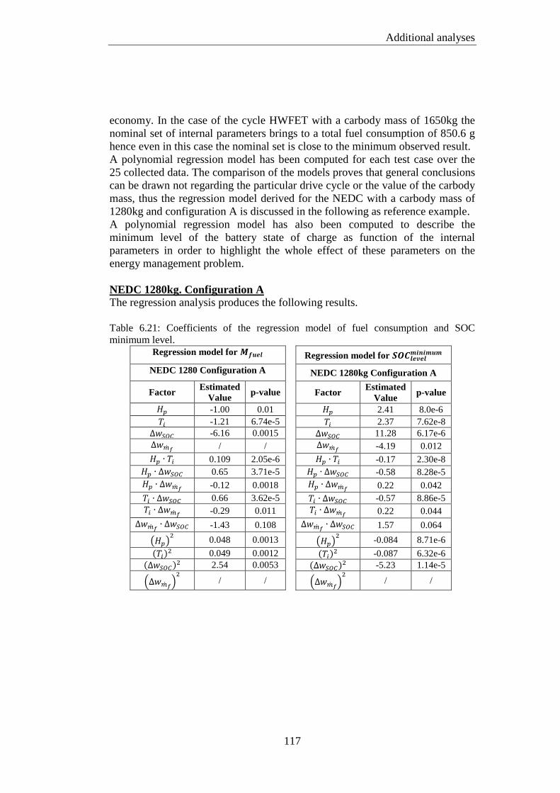
Additional analyses
117
economy. In the case of the cycle HWFET with a carbody mass of 1650kg the
nominal set of internal parameters brings to a total fuel consumption of 850.6 g
hence even in this case the nominal set is close to the minimum observed result.
A polynomial regression model has been computed for each test case over the
25 collected data. The comparison of the models proves that general conclusions
can be drawn not regarding the particular drive cycle or the value of the carbody
mass, thus the regression model derived for the NEDC with a carbody mass of
1280kg and configuration A is discussed in the following as reference example.
A polynomial regression model has also been computed to describe the
minimum level of the battery state of charge as function of the internal
parameters in order to highlight the whole effect of these parameters on the
energy management problem.
NEDC 1280kg. Configuration A
The regression analysis produces the following results.
Table 6.21: Coefficients of the regression model of fuel consumption and SOC
minimum level.
Regression model for
NEDC 1280 Configuration A
Factor Estimated
Value p-value
-1.00 0.01
-1.21 6.74e-5
-6.16 0.0015
/ /
0.109 2.05e-6
0.65 3.71e-5
-0.12 0.0018
0.66 3.62e-5
-0.29 0.011
-1.43 0.108
0.048 0.0013
0.049 0.0012
2.54 0.0053
/ /
Regression model for
NEDC 1280kg Configuration A
Factor Estimated
Value p-value
2.41 8.0e-6
2.37 7.62e-8
11.28 6.17e-6
-4.19 0.012
-0.17 2.30e-8
-0.58 8.28e-5
0.22 0.042
-0.57 8.86e-5
0.22 0.044
1.57 0.064
-0.084 8.71e-6
-0.087 6.32e-6
-5.23 1.14e-5
/ /

Chapter 6
118
Figure 6.24: Normal probability plot of the residuals.
The adjusted R2 is equal to 0.902. The normal probability plot, the p-value of the
statistical test for goodness of test fit and the value of the adjusted support
the idea that the regression model has a decent quality of regression. Analyzing
the regression coefficients it emerges that the influence of on total fuel
consumption is weaker than the other parameters; its linear and quadratic terms
have been removed from the regression model in order to achieve a good quality
of the regression. On the other hand the quadratic dependence of total fuel
consumption with respect to is strong; therefore the regression
coefficients seem to confirm the preliminary conclusions that have been
achieved from the 2-level full factorial DOE. It is interesting to plot the
observed total fuel consumption as function of the length of the prediction
horizon solely, thus the outcome of simulations number #17, #18 and #25 are
displayed in the following figure.

Additional analyses
119
Figure 6.25: Total fuel consumption for low, base and high level of Hp.
There is a length of the prediction horizon which seems to be optimal to achieve
the lowest fuel consumption. This conclusion is supported by the optimization
procedure which returns the set of internal parameters which minimizes only the
total fuel consumption. The genetic algorithm applied to the 25 observations
return the following optimal set:
point of minimum F2: 12 ; 0 ; -0.170879 ; 0.499773
minimum value of the object function : 492.6828
exitflag for F2 : 1 (6.1)
The optimal length of the prediction horizon is lower than the optimal value that
can be extracted from Figure 6.25 but it is necessary to consider that this figure
illustrates the total fuel consumption when the length of the prediction horizon is
the only variable which increases its value, whereas the optimization procedure
takes into account the cross-correlation terms. For instance the three
observations represented in Figure 6.25 refer to configurations where
however the optimal set defines an optimal value for this means that
these two variables are closely linked to each other and varying them in an
opposite way leads to similar final results. If the optimal set defined above is
compared to the nominal values of the internal parameters of the MPC strategy
it emerges that the main difference is in the optimal value of , thus the
penalty weight applied to the fuel mass flow rate increases. This is a reasonable
conclusion when the total fuel consumption is the only objective of the genetic
algorithm however Table 6.21 illustrates how this latter variable has a strong
influence on the minimum level reached by the battery state of charge
throughout the driving mission. If the optimal set were implemented in the
MPC-based control strategy it would produce a remarkable drop in the
equilibrium level of the battery state of charge.

Chapter 6
120
This reasoning is confirmed by a further analysis that has compared directly the
nominal set of values to the optimal one in (6.1) over NEDC with a carbody
mass of 1280kg.
Table 6.22: Comparison of the nominal against the optimal set of internal parameters. MPC strategy
Nominal 493.6 g 59.6 53.6
Optimal 493.0 g 57.2 51.0
Although the minimum level of the battery state of charge is higher than the
minimum threshold in both situations, it is important to mitigate the drop of
state of charge level in those cycles which involve strong accelerations therefore
it is advisable to keep the weight on the fuel mass flow rate equal to its base
value.
The analyses carried out with configuration B of the internal parameters prove
once more that it is useless to lengthen the prediction horizon more than 14 steps
since the total fuel consumption tends to increase. This result is shown in the
next two figures both for NEDC and for HWFET.
Figure 6.26: Total fuel consumption
as function of Hp. HWFET.
Figure 6.27: Total fuel consumption
as function of Hp. NEDC.
Collecting all information, the penalty weight and the length of the
prediction horizon seem to be the internal parameters which have the highest
influence on total fuel consumption and battery state of charge. The influence of
the parameter is closely related to the value of ; in fact both of them tend to
increase the importance of the deviation of the battery state of charge in the cost
function consequently similar results are achieved by increasing and
reducing simultaneously or vice versa. In conclusion the sensitivity analysis
on internal parameters reveals that:

Additional analyses
121
The nominal setting of internal parameters is adequate to achieve good
fuel economy over all reference drive cycles. This set manages to keep
the battery state of charge level inside the prescribed operating band
while reducing total fuel consumption with respect to a rule based
strategy.
It is not possible to find a different set of internal parameters values
which allows the control strategy to reduce further the total fuel
consumption as function of carbody mass.
and are the internal parameters which have the highest
influence on the performance of the strategy in terms of equilibrium
level of the battery state of charge and total fuel consumption.
The optimal value of is found in-between 11 and 14. It has been
observed during the tuning procedure that values lower than 10 produce
worse fuel consumption and very small value (i.e. lower than 6 samples)
produce an oscillatory behavior of the optimal solution.
Chapter 6
122
6.2.2 Integration of GPS/GIS
Thanks to the information provided by GPS and GIS it is possible to know the
instantaneous vehicle position on the earth surface and also map the slope of the
road that the vehicle is going to encounter. This information can be used to
predict the power request that the driver is likely to require in the near future.
The information on vehicle spatial position can be even more useful in the case
of a pubic mean of transportation like a bus which is supposed to repeat the
same driving route several times per day and therefore the stochastic properties
of future driving conditions can be foreseen with more accuracy than for a
passenger vehicle whose path cannot be known in advance. Assuming that the
average velocity of the bus and the average driver’s torque request have been
collected during driving under several repetitions of the same route, it is possible
to assign the average power request to each spatial position of the bus along a
specific route. If a further simplification is considered, namely the average
velocity profile coincides with the reference velocity profile of the considered
drive cycle and the average torque request corresponds to the torque request that
can be obtained running a simulation on the same drive cycle, then the desired
velocity and torque profiles can be provided to the MPC-based control strategy
as inputs. This represents undoubtedly an ideal situation but it enables to
evaluate the performance of the strategy when it works under the best possible
operating conditions. This part of the report deals with such a simplified model
and the aim is to investigate the role of the prediction on the numeric solution of
the optimization problem. In fact the choice to describe the torque request over
the prediction horizon according to an exponential decay is just one of the
available approaches, hence by using directly the real envelope of this variable it
is possible to judge if an alternative description may bring to a different
sequence of control actions.
For this purpose the profiles of the desired vehicle velocity and of the driver’s
torque request have been stored in look-up tables and used at each sampling
time as inputs to the control strategy. The optimization has been limited to a
prediction horizon of finite length thus the look-up tables return just a portion of
the trends of these two input variables. At sampling time vehicle position and
speed, driver’s requested torque are measured. In order to be able to predict
wheel torque and vehicle speed over the prediction horizon it is necessary to
know the correspondent positions of the vehicle center of mass. Vehicle position
is calculated after each prediction period by assuming that vehicle speed at one
sample remains constant over the following prediction period. Since the
prediction period is equal to 0.5s this assumption holds provided that the
instantaneous longitudinal acceleration is limited. This is the case for both
NEDC and HWFET where longitudinal acceleration exceeds rarely a magnitude
level of . The vehicle velocity and position are updated in parallel, and
once the new vehicle position is known a look-up tables is used to determine the

Additional analyses
123
torque request at the same sampling time. Eventually the values of vehicle
velocity and torque request are stored in two discrete vectors. It is therefore
assumed that in a first phase the control strategy communicates with the
navigation systems in order to acquire all these information and subsequently
the optimization problem is solved. This implies that an ideal situation is
considered where communication between MPC and navigation systems can
occur in a time period much smaller than the time required to solve the
optimization problem and thus the optimal values of the control variables can
always be found within a sampling period. All simulations have been carried out
testing the nominal control strategy characterized by the following parameters:
The vehicle parameters have been set equal to their nominal values. The cycles
NEDC and HWFET have been used as reference and a variable road profile has
been specified. The reference driving conditions of these two cycles are reported
in the next figures.
Figure 6.28: Road slope and velocity
profile for NEDC.
Figure 6.29: Road slope and velocity
profile for HWFET.
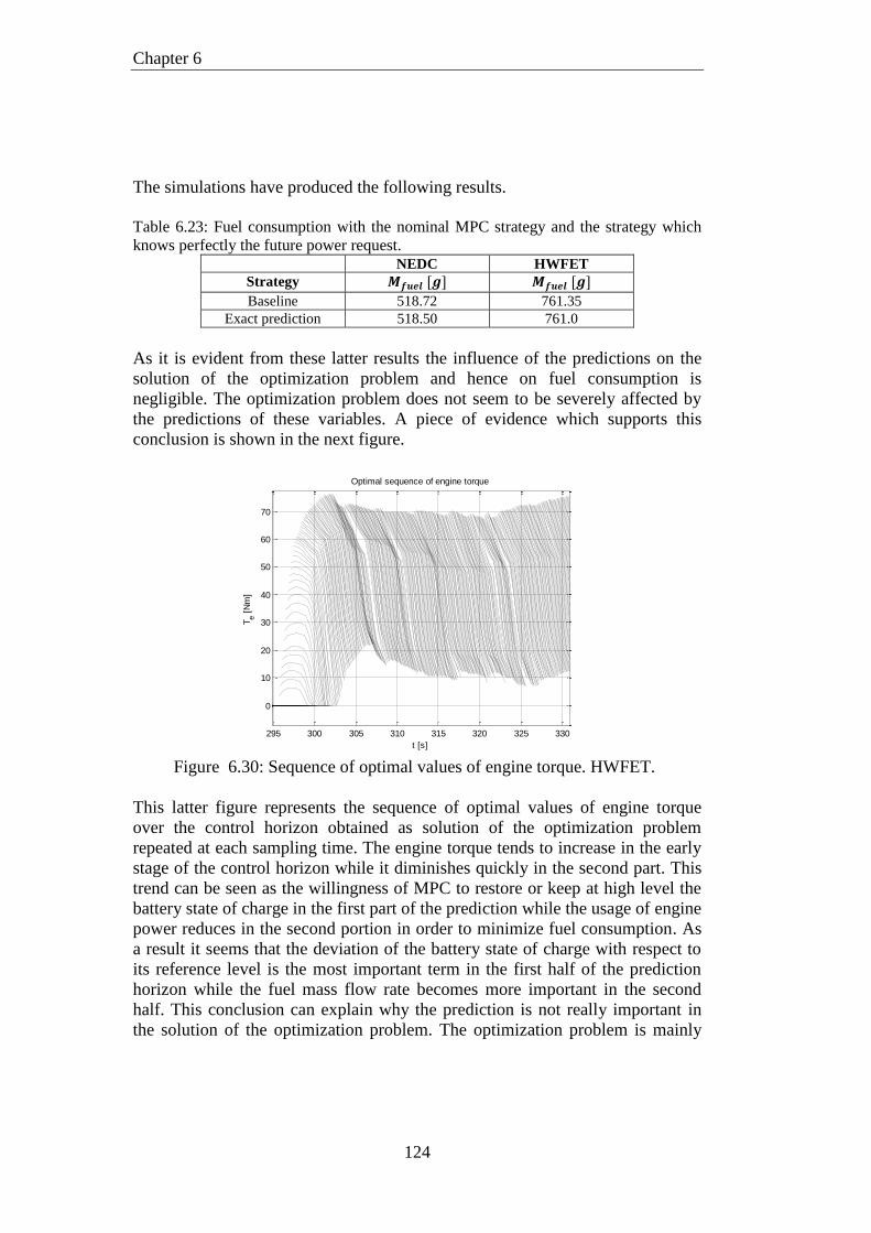
Chapter 6
124
The simulations have produced the following results.
Table 6.23: Fuel consumption with the nominal MPC strategy and the strategy which
knows perfectly the future power request. NEDC HWFET
Strategy
Baseline 518.72 761.35
Exact prediction 518.50 761.0
As it is evident from these latter results the influence of the predictions on the
solution of the optimization problem and hence on fuel consumption is
negligible. The optimization problem does not seem to be severely affected by
the predictions of these variables. A piece of evidence which supports this
conclusion is shown in the next figure.
Figure 6.30: Sequence of optimal values of engine torque. HWFET.
This latter figure represents the sequence of optimal values of engine torque
over the control horizon obtained as solution of the optimization problem
repeated at each sampling time. The engine torque tends to increase in the early
stage of the control horizon while it diminishes quickly in the second part. This
trend can be seen as the willingness of MPC to restore or keep at high level the
battery state of charge in the first part of the prediction while the usage of engine
power reduces in the second portion in order to minimize fuel consumption. As
a result it seems that the deviation of the battery state of charge with respect to
its reference level is the most important term in the first half of the prediction
horizon while the fuel mass flow rate becomes more important in the second
half. This conclusion can explain why the prediction is not really important in
the solution of the optimization problem. The optimization problem is mainly
295 300 305 310 315 320 325 330
0
10
20
30
40
50
60
70
Optimal sequence of engine torque
t [s]
Te [
Nm
]

Additional analyses
125
driven by the deviation of the battery state of charge and the level of power
request at the sampling time and not by their envelope along the prediction
horizon. Nonetheless the prediction is still important to guarantee the stability of
the strategy. In fact other simulations have shown how a length of the prediction
horizon shorter than 6 samples or a length of the control horizon shorter than 2
samples make the control action irregular and in some cases large fluctuations
appear either in the engine or in the generator optimal value.

Chapter 6
126

7 Conclusions and future works
This thesis work has shown the capability of a MPC-based energy management
control strategy to achieve better fuel economy than an optimized rule based
strategy implemented in Amesim®. The direct comparison with a rule based
strategy serves to quantify the performance of the MPC strategy. In particular
the improvement of overall efficiency seems to be larger for extra-urban driving,
rather than for urban driving. For instance the percentage reduction of fuel
consumption in UDDS urban cycle is equal to whereas it is equal to
in cycles NEDC, SC03, US06 respectively
which involve urban and extra urban conditions and high speed driving. The key
for this step ahead is a more efficient power split between battery and engine.
The engine provides the average power request while electric power supports
the engine in all driving situations to reduce the overall load and let this power
unit work in a region of low fuel consumption. The control action is obtained as
the solution of an optimization problem which makes use of a prediction of
future power request to decide the power split among the power units. However
the results have shown how the optimization problem is mostly driven by the
battery state of charge level and the driver’s torque request at sampling time. For
the same level of power request the engine torque is adjusted depending on the
state of discharge of the battery.
The sensitivity analysis focused on internal parameters has shown how the state
of charge equilibrium level varies significantly according to the setting of these
parameters while total fuel consumption is less influenced. It has been found
that the length of the prediction horizon, , and the variation of the penalty
weight of the deviation of the state of charge, , have the highest influence
on the outcome of the optimization problem. The optimal value of is around
11. By increasing fuel economy degrades. This is a first piece of evidence
that prediction is not fundamental but this latter conclusion is mostly supported
by the last analysis where additional information coming from GPS/GIS are
used to manipulate the control strategy. The correct torque and velocity profiles
have been assigned to the strategy but eventually the decisions taken by the
controller did not change. In particular, it has been proved that no matter the
torque description the optimal values of the control variables remain almost the
same; the magnitude of the optimal engine torque depends mainly on the
sampled value of the battery state of charge. This is a piece of advantage since
future power request is usually unknown. Furthermore it also indicates that the
control strategy is quite static and dominated by the deviation of the state of
charge level. Prediction is in any case fundamental to solve the optimization
problem and stabilize the control strategy however if additional information on
Chapter 7
128
traffic, road conditions were available, they should be exploited by another
controller which is placed above MPC and can actively modify some parameters
of the MPC control strategy like for instance the reference value of the battery
state of charge as function of road slope.
In this thesis work the control strategy has been developed in order to take into
account few issues related to drivability. In particular a typical problem
associated to a HEV is engine starting and stopping which usually occurs when
the vehicle is moving and it causes vibrations which degrade the on-board
comfort. The amount of vibrations have been reduced by controlling the
dynamics of these events through the generator torque. The results have shown
how the oscillations related to engine starting and stopping can be significantly
reduced when the vehicle supervisory controller can directly adjust this latter
control variable. The standard norm ISO 2631-5 prescribes that the equivalent
acceleration felt by the passenger should be lower than ; the strategy
manages to start and stop the engine rotation without causing a total acceleration
higher than this threshold value. The comfort analysis has been carried out in the
cycle NEDC and it thus shows the capability of the strategy to include
objectives defined by different fields.
Another piece of advantage is that the strategy can be applied to any drive cycle
and none parameter has been tuned for specific driving conditions. From this
point of view this strategy is more robust than, for instance, A-ECMS where the
equivalency factor depends on the driving scenario.
Possible drawbacks have been identified in the linear time varying approach
which implies to use a linearized state space form at each sampling time.
Linearization introduces some errors like for instance the prediction of electric
machines power loss. It has been shown how the linearization of the nonlinear
function which describes the power loss inside the electric generator can
produce an oscillatory behavior of the optimal control action defined by the
MPC strategy. This problem has been solved by penalizing the variation of the
electric generator output torque when the engine is working and the generator
rotor angular velocity approaches the null value. However this idea introduces a
penalty weight that is based on the value of the generator angular velocity at the
sampling time thus it may suffer from measurement noise in the input data.
Moreover the actual implementation of a MPC strategy for energy management
of a hybrid vehicle still retains some doubts. In fact the values of the control
inputs are determined through numerical solution of an optimization problem
and the solver should be fast enough to find an optimal solution within a
sampling period. In this thesis a sampling period of 0.1s has been used but
similar results can be obtained using a slightly longer sampling period equal to
0.2s. The numerical simulations have shown that the time required to find a
Conclusions and future works
129
suitable optimal solution is shorter than the sampling period, thus the
implementation of the strategy on the calculator did not represent an issue. The
optimized active set algorithm has been developed to be suitable for real time
purposes. Nevertheless it is necessary to investigate more how the strategy
should behave when, for any reason, it is not possible to find a solution in view
of real time application. Furthermore Model Predictive Control is a model based
approach meaning that it is always necessary to define a simple but reliable
model of the dynamic system and any modification applied to the powertrain
may require to develop a complete new model.
Further improvements may appeal to the extension of the cost function in order
to include the emission rates of pollutants and analyze how the operating point
of the engine changes when both fuel consumption and pollutant emissions
should be minimized. Secondly it would be interesting to refine the analysis of
the implementation of navigation systems to improve the optimization problem
by designing a high level controller placed above the vehicle supervisory
controller in the hierarchical structure of the energy management of a hybrid
electric vehicle. Since the solution to the optimization problem seems to be
mainly driven by the level of the battery state of charge and power request at the
sampling time, it is worth to compare the MPC-based control strategy against A-
ECMS which solves an instantaneous optimization problem.

Chapter 7
130
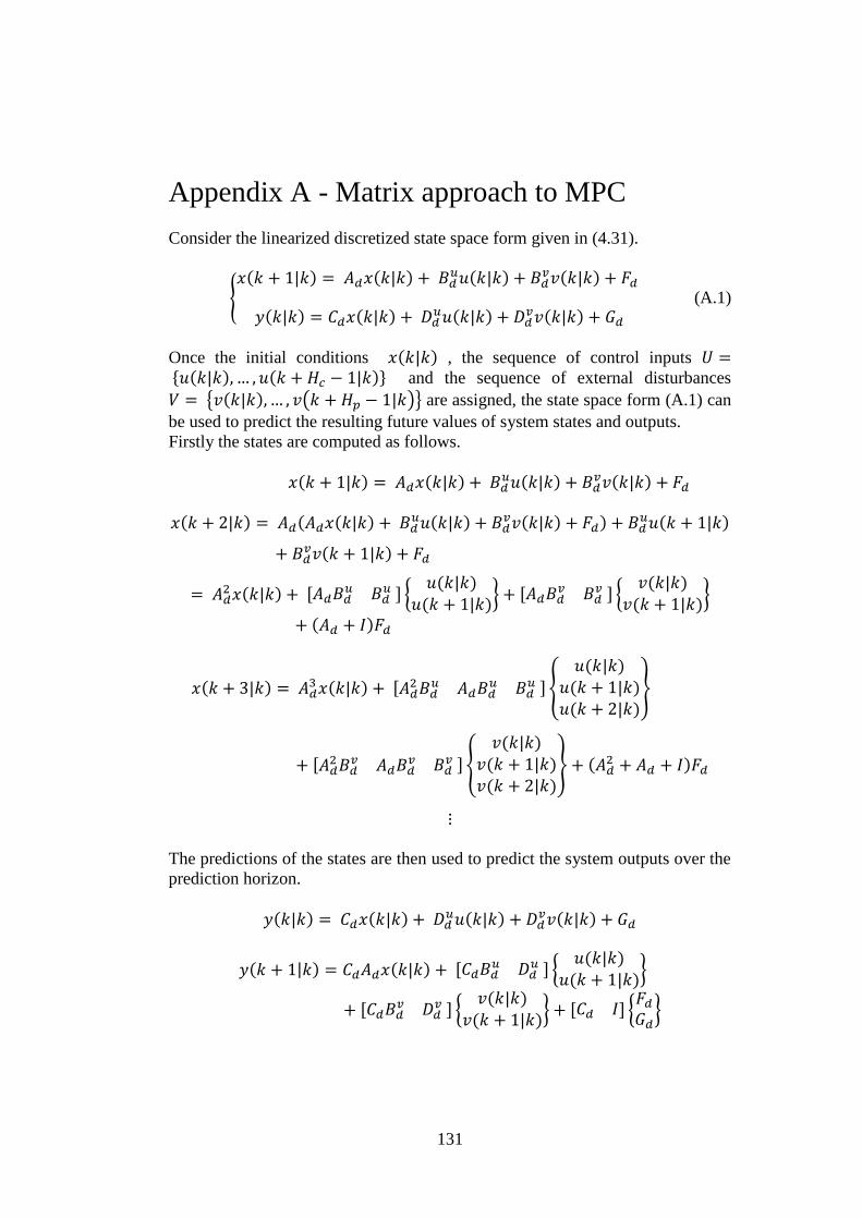
131
Appendix A - Matrix approach to MPC
Consider the linearized discretized state space form given in (4.31).
(A.1)
Once the initial conditions , the sequence of control inputs and the sequence of external disturbances
are assigned, the state space form (A.1) can
be used to predict the resulting future values of system states and outputs.
Firstly the states are computed as follows.
The predictions of the states are then used to predict the system outputs over the
prediction horizon.

Appendix A
132
Using a matrix formulation, the sequence of system outputs over the prediction
horizon can be formulated as follows.
(A.2)
where: sequence of known measured disturbances
sequence of predicted states
sequence of predicted outputs
sequence of control inputs to be optimized
measured system state at the sampling time k
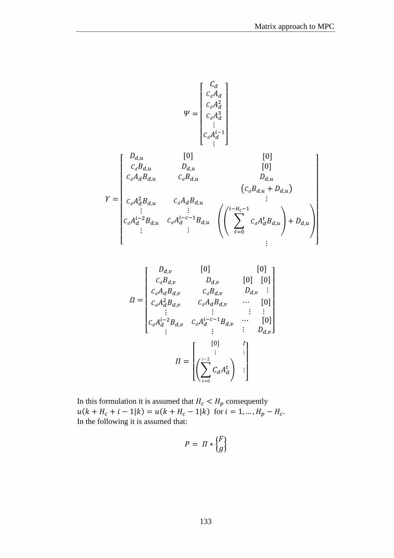
Matrix approach to MPC
133
In this formulation it is assumed that consequently
for .
In the following it is assumed that:

Appendix A
134
Constraints
Suppose that the constraints for one sample in the prediction and in the control
horizon respectively are expressed in matrix form as follows:
The constraints are enforced along the whole prediction and control horizons
through the sequences of control inputs and system outputs; block diagonal
matrices are created.
A more compact form:
By using (A.2) in place of the sequence of system outputs, it is possible to
express all constraints with respect to the sequence of control inputs.

Matrix approach to MPC
135
Eventually the standard expression of inequalities constraints can be achieved
by collecting all matrices and all vectors as follows.
Cost function
The discrete expression of the cost function for the energy management problem
includes a summation along the control horizon and a summation along the
prediction horizon.
A more compact expression is achieved by introducing diagonal matrices of the
weights and vectors of system outputs and states.
By using the sequences of system outputs and control inputs in place of
summations, the following final matrix formulation is obtained.
(A.3)
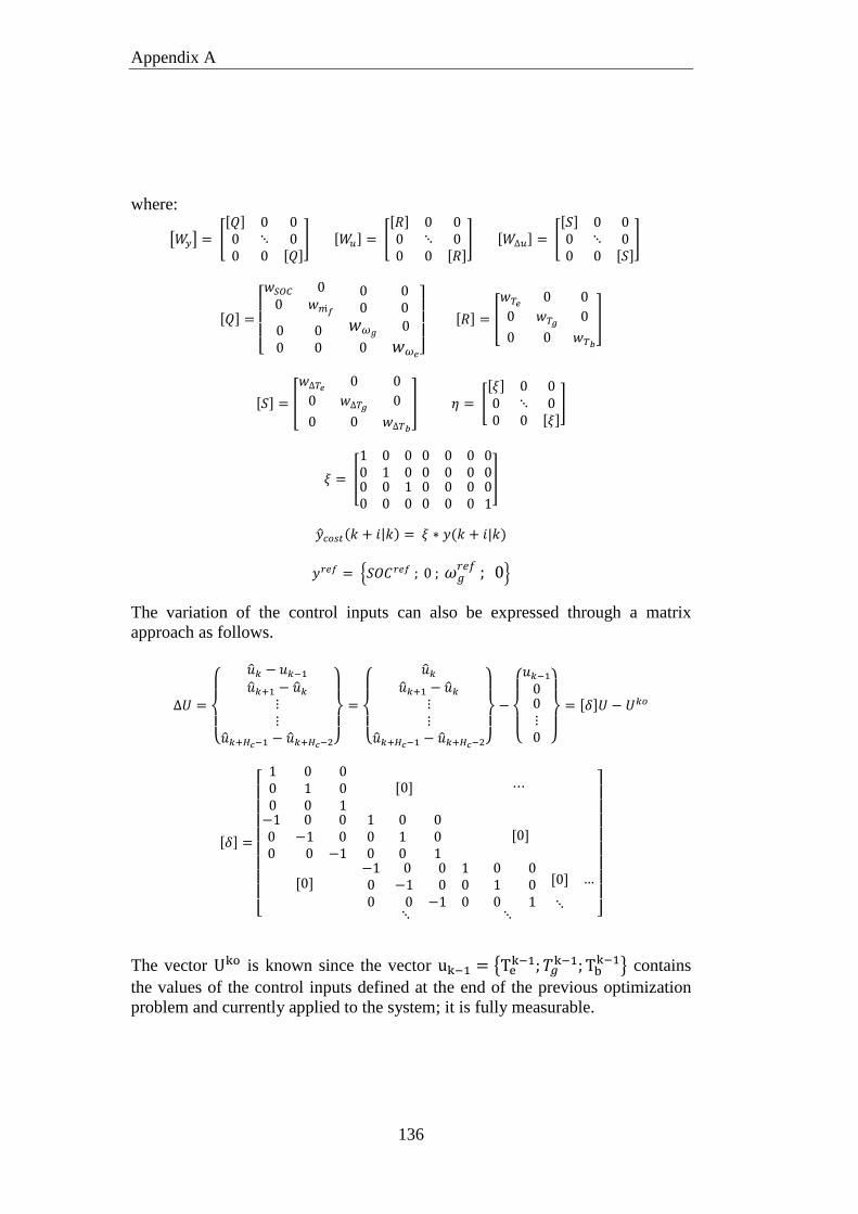
Appendix A
136
where:
The variation of the control inputs can also be expressed through a matrix
approach as follows.
The vector is known since the vector
contains
the values of the control inputs defined at the end of the previous optimization
problem and currently applied to the system; it is fully measurable.

Matrix approach to MPC
137
The equation (A.3) can be expanded using the definitions given above and
eventually the whole expressions of matrix H and vector q are computed as
follows.
The constant term includes all terms that do not multiple .

Appendix A
138

139
Appendix B - Sensitivity analysis and RSM
Suppose the relation between inputs and outputs of a system were known in a
closed loop form as [27]:
(B.1)
where y represents in the general case a vector of outputs while X represents
generally a vector of inputs, then a sensitivity coefficient would be defined as
the rate of change of one system outputs with respect to a variation of one
system inputs.
(B.2)
In a mathematical form it would correspond to the partial derivative of the
function with respect to the i-th input, evaluated at a specific set point .
The function is generally unknown in closed loop form consequently some
techniques have been developed in order to rank the influence of each input
parameter on each system output on the basis of observations collected during
some tests on the system. The mathematical approach which applies one of these
techniques is called Sensitivity Analysis and it is widely applied in engineering
design in order to identify which parameters or independent variables affect the
most the response of a system. Once these parameters, variables have been
identified their values can be adjusted in order to obtain a desired response of
the system. It can also highlight the robustness of the system with respect to
parameter uncertainty. Since most of the techniques determine the sensitivity
coefficients according to various formulations of (B.2), they rely on the
assumption of linear response of the system and therefore the results from a
sensitivity analysis are limited to the region of the input domain which was
explored during the tests. Furthermore it is likely that the observations may
depend on the particular set point that is selected as base configuration so the
analysis should be repeated using different initial set points, in particular if the
system response is assumed to be nonlinear. Depending on whether the data
come from experimental runs or from computer based simulations, the
techniques to set up a sensitivity analysis may vary because computer based
simulations lack of the variability in the input data. In both cases the available
resources (money, time, knowledge of the system etc…) to carry out a set of
runs are usually limited and this prevents from running a large set of
configurations. For this reason different techniques are available to identify the
relations among inputs and outputs ranging from simple procedures to more
complex mathematical approaches [27]. The one-at-a-time analysis (OAT)

Appendix B
140
represents the simplest and the least accurate design for sensitivity analysis since
it implies to vary one input parameter at a time while all other parameters are
kept fixed to their base values; in this way the change in the system response can
be undoubtedly related to the change in a parameter level. The main drawback
of an OAT analysis is represented by the impossibility to capture any correlation
among the input parameters which may affect severely the system response. In
fact the effect of a parameter on system response depends generally on the
values assumed by the other parameters of the model. For this reason the OAT
analysis is regarded to as a Local sensitivity analysis while Global sensitivity
analysis involves changing simultaneously the levels of all parameters or at least
part of them; the techniques which are presented here below belong to this latter
class. Design of experiment (DOE) represents one step ahead towards a better
description of the behavior of the system. This technique provides for creating a
list of configurations to be tested where each parameter assumes a different
level. It is based on a set of principles:
comparison: all results are compared to a base case.
randomization: namely the process which determines the parameter
configurations to be tested. This process is fundamental because all
configurations should be selected in order to be independent on one
another.
replication: in case of a process with a stochastic outcome, a
configuration may be analyzed a number of times in order to evaluate the
variability associated to random error on the output
factorial experiment: each parameter can change level independently on
the level assumed by the other factors
Thanks to the simultaneous variation of parameters level it is possible to draw
some conclusions on main effects and correlation effects of parameters on
system response. The list of parameters configurations is created according to
different sampling approaches and typical methods are factorial design, CCD
and D-design. The list is stored in a proper matrix, called design matrix.
Factorial design is usually applied to have a first understanding of input-output
relations. Depending on the structure of the list, either a full or a fractional
factorial design can be carried out meaning that in the former case all main
effects and all interaction effects can be successfully isolated while in the latter
case the parameter main effects can be influenced by any correlations among
two or more parameters. However since a fractional factorial design requires a
smaller number of runs and the influence of high order correlations is usually
weak on system response, this analysis is usually preferred. A design matrix is
classified according to its resolution, namely the degree to which estimated main
effects are confounded with estimated interaction effects.
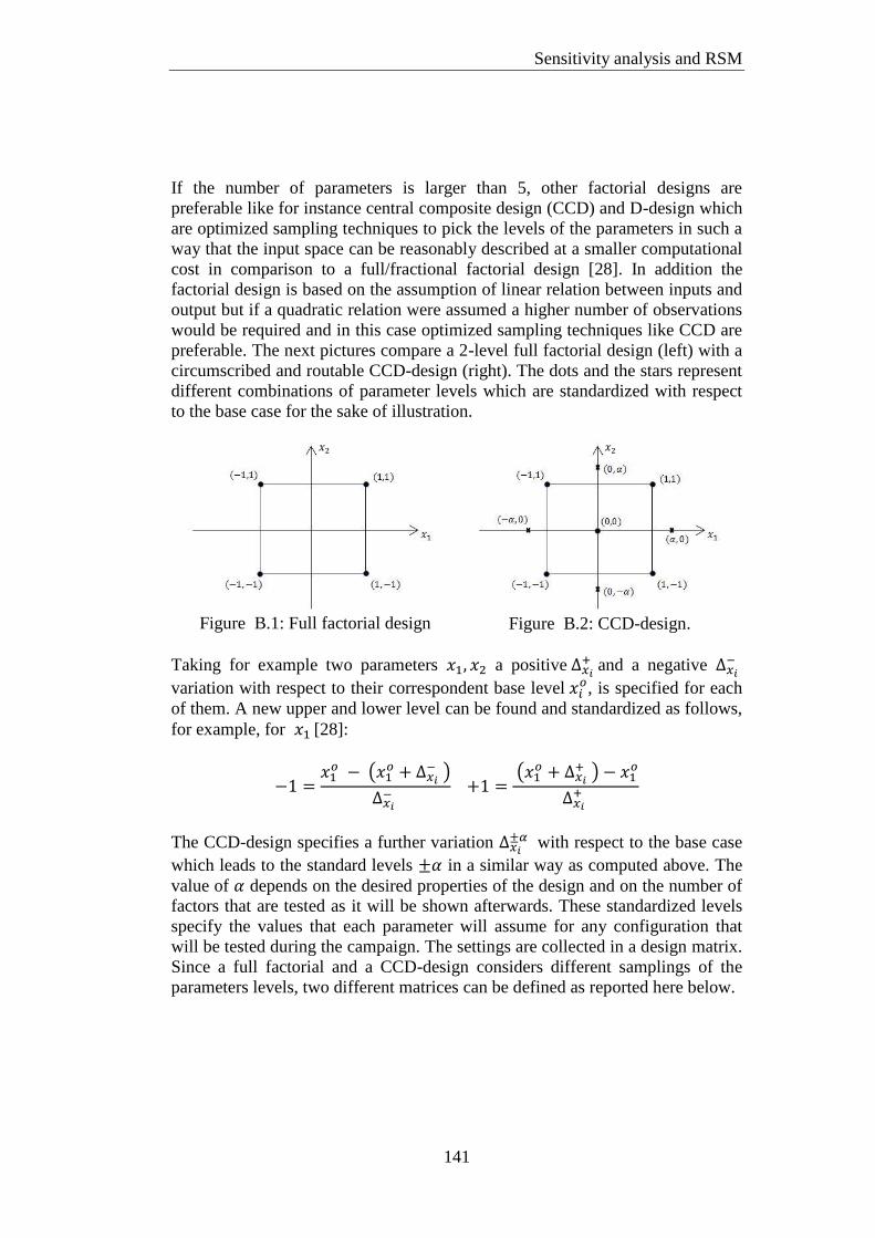
Sensitivity analysis and RSM
141
If the number of parameters is larger than 5, other factorial designs are
preferable like for instance central composite design (CCD) and D-design which
are optimized sampling techniques to pick the levels of the parameters in such a
way that the input space can be reasonably described at a smaller computational
cost in comparison to a full/fractional factorial design [28]. In addition the
factorial design is based on the assumption of linear relation between inputs and
output but if a quadratic relation were assumed a higher number of observations
would be required and in this case optimized sampling techniques like CCD are
preferable. The next pictures compare a 2-level full factorial design (left) with a
circumscribed and routable CCD-design (right). The dots and the stars represent
different combinations of parameter levels which are standardized with respect
to the base case for the sake of illustration.
Figure B.1: Full factorial design
Figure B.2: CCD-design.
Taking for example two parameters a positive
and a negative
variation with respect to their correspondent base level , is specified for each
of them. A new upper and lower level can be found and standardized as follows,
for example, for [28]:
The CCD-design specifies a further variation
with respect to the base case
which leads to the standard levels in a similar way as computed above. The
value of depends on the desired properties of the design and on the number of
factors that are tested as it will be shown afterwards. These standardized levels
specify the values that each parameter will assume for any configuration that
will be tested during the campaign. The settings are collected in a design matrix.
Since a full factorial and a CCD-design considers different samplings of the
parameters levels, two different matrices can be defined as reported here below.

Appendix B
142
Table B.1: Design matrix of full
factorial
test
#1 -1 +1
#2 +1 +1
#3 -1 -1
#4 +1 -1
Table B.2: Design matrix of CCD-
design
test
#1 -1 +1
#2 +1 +1
#3 -1 -1
#4 +1 -1
#5 - 0
#6 + 0
#7 0 -
#8 0 +
#9 0 0
This example shows how the design matrix of a CCD-design is equivalent to the
design matrix of a 2-level full factorial design plus additional star and central
points. These additional points serve to calculate the curvature of the response
surface, the central point is also important to assess the lack of fit of a regression
model. Therefore the benefit to apply a CCD-design with respect to a full
factorial design is more evident as the number of parameters increases. For
instance if four parameters has to be tested on 3 levels each, a full factorial
design would require runs while runs are necessary for
a CCD-design where indicates the number of runs that should be
repeated for the base configuration. This latter value can be equal to 1 for
deterministic processes while it is usually much greater than one ( for
experimental based runs since the variability in the process outcome at the
center point can be used as a measure of the lack of fit. As the previous design
matrices show, a CCD-design always takes more levels for each parameter even
for a simple test case like the one considered here. A design matrix is created
with the property of being orthogonal, namely none parameter configuration can
appear twice within the same sequence of runs. However this matrix specifies
the levels for each parameter in any configuration consequently the
experimentalist is free to upset the order and to repeat each configuration a
number of times in order to have a measure of the variance in the outputs. In the
case of a CCD-design further properties can be achieved depending on how the
design matrix is built:
type:
circumscribed: the star points are placed at distance from the
center point and represent new extreme levels for the parameters.
The value of depends on the desired properties of the design
and on the number of factors involved in the analysis. This type
of test explores the largest input space, it has a spherical
symmetry and it defines 5 levels for each parameter.

Sensitivity analysis and RSM
143
inscribed: this design can be obtained from a circumscribed one
by dividing the star point for , namely the star points are added
in such a way that they do not exceed the extreme values impose
by the original factorial levels. This type comprises 5 levels for
each factor.
face centered: in this design so just three levels for each
factor are tested. This type explores the smallest input space since
the value of delimits the domain to be considered.
rotatability: a design matrix is rotatable if the variance of the predicted
output response at an input point X depends only on the distance between
X and the center point. This property is important to apply a response
surface methodology because it implies that the observations do not
depend on the direction followed from the center point to define a
parameter level.
The latter property holds by assigning a desired value of . The following
formula reports the desired value of as function of the number of factorial runs
which eventually depends on the number of parameters:
The number of experimental runs is related to either a full or a fractional
factorial because the design matrix of a CCD-design is built upon a 2-level full
or fractional design augmented with a number of star and central points. The
following figures report the parameters levels for a 2-factor CCD-design for
either a circumscribed or a face centered or an inscribed design.

Appendix B
144
circumscribed face centered inscribed
Figure B.3: The test configurations taken by three different design matrices.
In an experimental based design the repetitions of runs at the center point allows
assessing the lack of fit, namely if the analysis omits some important terms in
the regression model. The lack of fit represents a steady error due to poor
regression model and it is a different source of error than the random error due
to random uncertainty.
The most advanced approach to analyze input-output relations is represented by
random sampling techniques which are referred to as Monte Carlo simulations.
In this approach the input space of parameters is better described since each
parameter can assume several levels and the correspondent values are picked at
random from the correspondent parameter domain. Due to the fact that more
observations are available and parameters values are picked randomly about the
correspondent base value it is possible to calculate the sensitivity coefficients
using the analysis of variance or other detailed mathematical calculations like
Fourier amplitude sensitivity. A base case is always specified and values are
picked in the neighborhood; efficient optimized random sampling techniques
like optimized Latin hypercube are employed to guarantee that the input space
can be described well. Contrary to the previous case, the experimentalist has
only to define the boundaries of the input space and not the discrete levels of
each parameter. The drawback of this latter approach is the long time required
for the whole simulation or experimentation due to the increased number of
combinations to be evaluated. For experimental design it is often unfeasible
applying this approach and even computer based design may become too long if
the model is complex. Monte Carlo methods are applied to a variety of problems
and their application to sensitivity analysis is mostly focused on the
determination of a suitable regression model. They can also be directly applied
to evaluate the robustness of a control strategy towards uncertainty in model
parameters and measurement noise.
(1,1) (1,1)
(1,0) (-1,0)
(0,1)
(0,-1) (1,-1) (-1,-1)
(-1,1) (-1,1)
(-1,-1) (1,-1)

Sensitivity analysis and RSM
145
The regression analysis provides the most comprehensive sensitivity measure by
deriving a mathematical regression model of the observations which can relate
the inputs to the output. The unknowns of a regression analysis are the
regression coefficients and a regression model is defined either linear or
nonlinear depending on the relation between the system response and the
regression coefficients. A linear regression model can include nonlinear
relations between independent variables and system response. This model can be
specified by any possible mathematical function but polynomial curves or
surfaces of independent variables are utilized for the sake of simplicity.
Moreover the resource available to conduct experimental runs are usually
limited therefore for practical applications it is rare to have enough observations
to derive a polynomial response surface of order higher than 2. A second order
polynomial gives the possibility to find an optimum of the system response;
nevertheless a response surface is always limited to a small domain around the
initial base case meaning that inference on system response should be avoided
outside the domain used to get the observations. The magnitude of the
regression coefficients is a direct ranking of parameter influence over the system
output; if the regression surface is to be used to rank the parameter influence the
regression coefficients are usually standardized in order to take into account the
relative units and place all parameters on an equal level. For the sake of
simplicity it is common to start guessing a linear regression model. Linearity is
assumed for the regression coefficients while each independent input variable
can appear in the regression model through a nonlinear function. Once a suitable
model is guessed, the regression coefficients are calculated by means of least
square method in order to minimize the distance between the observed values
and the values obtained from the regression model at the correspondent input
configurations. A second order polynomial regression model can usually assume
a form similar to the following one:
(B.3)
where with are the regression coefficients while , with
, are the independent variables. Here represents the response of the
system. In order to assess the adequacy of the regression model, statistical test
fit is usually applied. The analysis of variance (ANOVA) is an established
technique to judge if there is high probability that the hypothesized regression
model matches the observed values at a certain significance level.
ANOVA relies on three main assumptions:
the levels of an independent variable are not influenced by the levels of
the other input variables

Appendix B
146
the residuals coming from the regression are assumed to be normally
distributed having zero mean
the variance in the data is assumed to remain constant among different
populations of the input data
The first assumption can be validated by the user when the factor levels are
chosen while the third assumption does not represent an issue when computer
based simulations are considered due to the lack of intrinsic uncertainty in input
data. On the other hand the second assumption can be used as starting point to
check the adequacy of the regression model. Once the regression coefficients are
calculated, the residuals of regression can be computed as:
where is the system response obtained at the i-th configuration of the
parameters using the regression model and is the i-th observation. If the
second assumption holds a normal probability plot of the residuals should
produce a plot where all points lie on a straight line. If the points are not ordered
on a line but are randomly spread then it can be concluded that the regression
model has poor quality. A more refined investigation appeals to hypothesis
testing where through a statistical approach it is possible to infer some
conclusions on regression coefficients. The null hypothesis that should be
rejected is that the k-th regression coefficient is null against the hypothesis
that it is not null. ANOVA uses an F-test to evaluate this hypothesis and
conclusions can be drawn on the null hypothesis from the p-value of the test. It
is customary to assume that a p-value smaller than 0.05 sets moderate or high
evidence against the null hypothesis, namely that there is high probability that
the null hypothesis is wrong and the k-th regression coefficient is not null in the
regression model. The threshold value 0.05 is called “significance of the test”.
This hypothesis testing evaluates the hypothesis of having a constant model
against a linear model.

Appendix C - Standard drive cycles
The velocity profiles of the standard drive cycles that have been considered
throughout the analysis are reported below.
NEDC
o Road profile: flat
o Length of the cycle: 11.010 km
Figure C.1: Reference velocity profile of cycle NEDC
HWFET o Road profile: flat
o Length of the cycle: 16.501 km
Figure C.2: Reference velocity profile of cycle HWFET

Appendix C
148
SC03 o Road profile: flat
o Length of the cycle: 5.758 km
Figure C.3: Reference velocity profile of cycle SC03
UDDS
o Road profile: flat
o Length of the cycle: 11.985 km
Figure C.4: Reference velocity profile of cycle UDDS

Standard drive cycles
149
US06
o Road profile: flat
o Length of the cycle: 12.882 km
Figure C.5: Reference velocity profile of cycle US06

Appendix C
150

Bibliography
[1] I. Husain, Electric and Hybrid vehicles. Design and Fundamentals, Second
Edition ed., CRC Press.
[2] G. Ferrari, Motori a combustione interna, Il Capitello.
[3] K. Govindswamy, T. Wellmann and G. Eisele, “Aspects of NVH
integration in Hybrid Vehicles,” SAE International.
[4] P. J. Møller, “Seminar on Electric vehicle,” DTU, Lyngby, Denmark, 2011.
[5] L. Serrao, “"A comparative analysis of energy management strategies for
hybrid electric vehicles.",” Electronic Thesis or Dissertation. Ohio State
University, 2009. https://etd.ohiolink.edu/.
[6] P. Pisu and G. Rizzoni, “"A Comparative Study Of Supervisory Control
Strategies for Hybrid Electric Vehicles,",” Control Systems Technology,
IEEE Transactions on, vol. 15, no. 3, pp. 506-518, May 2007.
[7] A. Sciarretta and L. Guzzella, “Control of Hybrid electric vehicles,”
Control of Systems, IEEE, vol. 27, no. 2, pp. 60-70, April 2007.
[8] D. V. Ngo, T. Hofman, M. Steinbuch and Serrarens, “"An optimal control-
based algorithm for Hybrid Electric Vehicle using preview route
information,",” American Control Conference (ACC), pp. 5818-5823, June
30th 2010-July 2nd 2010.
[9] S. P. B. E. L. Johannesson, “"Predictive energy management of a 4QT
series-parallel hybrid electric bus",” Control Engineering Practice, vol. 17,
pp. 1440-1453, 2009.
[10] G. Ripaccioli, D. Bernardini, S. Di Cairano, A. Bemporad e I.
Kolmanovsky, «"A stochastic model predictive control approach for series
hybrid electric vehicle power management,",» American Control
Conference (ACC), pp. 5844-5849, June 30 2010-July 2 2010.
[11] R. G. Y. S. B. Musardo C, «“A-ECMS: An Adaptive Algorithm for Hybrid
Electric Vehicle Energy Management”,» European Journal of Control ,
vol. 11, pp. 509-524, 2005.
[12] R. Beck, F. Richert, A. Bollig, D. Abel, S. Saenger, K. Neil, T. Scholt e K.
Noreikat, «"Model Predictive Control of a Parallel Hybrid Vehicle
Drivetrain,",» Decision and Control, 2005 European Control Conference.
CDC-ECC '05. 44th IEEE Conference, vol. 12, n. 15, pp. 2670-2675.
[13] L. d. Re, Automotive model predictive control: Models, Methods and
Applications, Springer-Verlag.
[14] S. Di Cairano, W. Liang, I. Kolmanovsky, M. Kuang and A. Phillips,
“"Engine power smoothing energy management strategy for a series hybrid
152
electric vehicle,",” American Control Conference (ACC), pp. 2101-2106,
June 29th 2011, July 1st 2011.
[15] H. A. Vahidi, A. Phillips, M. Kuang, I. Kolmanovsky e S. Di Cairano,
«"MPC-Based Energy Management of a Power-Split Hybrid Electric
Vehicle,",» Control Systems Technology, IEEE Transactions, vol. 20, n. 3,
pp. 593-603, May 2012.
[16] M. M. a. T. K. K. Yu, «"Model predictive control of a power-split hybrid
electric vehicle system, ",» Artificial Life and Robotics, vol. 17, n. 2, pp.
221-226, Dec 2012.
[17] L. Johannesson, M. Asbogard e B. Egardt, «"Assessing the Potential of
Predictive Control for Hybrid Vehicle Powertrains Using Stochastic
Dynamic Programming,",» Intelligent Transportation Systems, IEEE
Transactions , vol. 18, n. 1, pp. 71-83, March 2007.
[18] D. Opila, D. Aswani, R. McGee, J. Cook e J. Grizzle, «"Incorporating
drivability metrics into optimal energy management strategies for Hybrid
Vehicles,",» Decision and Control, 2008. CDC 2008. 47th IEEE
Conference, vol. 9, n. 11, pp. 4382-4389, Dec 2008.
[19] A. S. b. LMS, “Amesim User's Guide,” 2012.
[20] F. U. e. al., “Derivation and Experimental Validation of a Power-Split
Hybrid Electric Vehicle Model,” IEEE Transactions on vehicular
technology, vol. 55, no. 6, pp. 1734-1747, November 2006.
[21] L. Guzzella and A. Sciarretta, Vehicle Propulsion Systems. Introduction to
Modeling and Optimization., Third Edition ed., Springer-Verlag, 2013.
[22] Toyota, «Toyota Hybrid system THS II,» May 2003.
[23] J. Maciejowski, Predictive control with constraints, Prentice Hall, 2002.
[24] L. Wang, Model Predictive Control System Design and Implementation
Using Matlab®, Springer, 2009.
[25] Ferreau, Kirches, Potschka, Bock and Diehl, “qpOASES: A parametric
active-set algorithm for quadratic programming,” Mathematical
Programming Computation, 2014.
[26] “ISO 2631-1:1997 Mechanical vibration and shock - Evaluation of human
exposure to whole-body vibration,” International Organisation for
Standardisation, Schweiz, 1997.
[27] Q. Huang e H. Wang, «Fundamental Study of Jerk: Evaluation of Shift
Quality and Ride Comfort.,» SAE International, 2004.
[28] A. Fassò and P. Perri, “Sensitivity analysis,” Encyclopedia of
Environmetrics, 2006.
[29] N. Bradley, The Response Surface Methodology, Thesis in Applied
mathematics & computer science, 2007.

153


