POLITECNICO DI MILANO · Introduzione 1.1 L’importanza del mixing Attualmente il mixing come...

POLITECNICO DI MILANO

FACOLTA DI INGEGNERIA INDUSTRIALE

Corso di Laurea in Ingegneria Aeronautica

Experimental measurement of the efficiency of turbulent mixing

for non-conventional mixers

Relatore: Laureando:

Prof. Maurizio Quadrio Davide ArnoneCorrelatore: Matr.754872Prof. Pietro PoesioTutor:

Dott. Stefano Farise

Anno Accademico 2012-2013

Alla mia famigliaAi miei nipotiAi miei amici

Contents

Contents i

List of Figures iii

1 Introduzione 1

1.1 L’importanza del mixing . . . . . . . . . . . . . . . . . . . . . . . . 1

1.2 Motivazioni del lavoro di tesi . . . . . . . . . . . . . . . . . . . . . 2

2 Percorso di ricerca 3

3 Introduction 7

3.1 The importance of mixing . . . . . . . . . . . . . . . . . . . . . . . 7

3.2 Reasons of the research work . . . . . . . . . . . . . . . . . . . . . 7

3.3 Thesis structure . . . . . . . . . . . . . . . . . . . . . . . . . . . . . 8

4 Preliminary studies 9

4.1 Mixing . . . . . . . . . . . . . . . . . . . . . . . . . . . . . . . . . . 9

4.1.1 Mixer for liquids . . . . . . . . . . . . . . . . . . . . . . . . 9

4.1.2 Experimental tests on mixers . . . . . . . . . . . . . . . . . 11

4.1.3 Dimensionless numbers . . . . . . . . . . . . . . . . . . . . 12

4.2 Theory of heat transfer in semi-infinite plane . . . . . . . . . . . . 14

5 Experimental Setup 19

5.1 Design choises . . . . . . . . . . . . . . . . . . . . . . . . . . . . . . 19

5.2 3D model . . . . . . . . . . . . . . . . . . . . . . . . . . . . . . . . 20

5.3 Configurations of the mixer . . . . . . . . . . . . . . . . . . . . . . 21

5.4 Power supply . . . . . . . . . . . . . . . . . . . . . . . . . . . . . . 22

5.5 Heating and cooling system . . . . . . . . . . . . . . . . . . . . . . 22

5.6 Motor . . . . . . . . . . . . . . . . . . . . . . . . . . . . . . . . . . 22

5.7 Sensors . . . . . . . . . . . . . . . . . . . . . . . . . . . . . . . . . 24

5.7.1 Thermocouples . . . . . . . . . . . . . . . . . . . . . . . . . 24

5.7.2 Current sensor . . . . . . . . . . . . . . . . . . . . . . . . . 24

5.7.3 Encoder . . . . . . . . . . . . . . . . . . . . . . . . . . . . . 25

5.8 Acquisition system . . . . . . . . . . . . . . . . . . . . . . . . . . . 26

i

ii CONTENTS

5.8.1 LabVIEW . . . . . . . . . . . . . . . . . . . . . . . . . . . . 265.8.2 NI USB-6009 . . . . . . . . . . . . . . . . . . . . . . . . . . 275.8.3 NI9213 and NI9205 . . . . . . . . . . . . . . . . . . . . . . . 27

5.9 Matlab . . . . . . . . . . . . . . . . . . . . . . . . . . . . . . . . . . 295.9.1 Post-process of temperature data . . . . . . . . . . . . . . . 295.9.2 Post-process of motor data . . . . . . . . . . . . . . . . . . 30

5.10 Experimental Procedure . . . . . . . . . . . . . . . . . . . . . . . . 325.11 Diagram of the experimental setup . . . . . . . . . . . . . . . . . . 33

6 Validation 35

6.1 Test of the thermocouples . . . . . . . . . . . . . . . . . . . . . . . 356.2 Cooling test . . . . . . . . . . . . . . . . . . . . . . . . . . . . . . . 416.3 Heating test . . . . . . . . . . . . . . . . . . . . . . . . . . . . . . . 416.4 Mixing time procedure test . . . . . . . . . . . . . . . . . . . . . . 446.5 Test of the experimental procedure . . . . . . . . . . . . . . . . . . 476.6 Calibration of the current sensor . . . . . . . . . . . . . . . . . . . 486.7 Estimation errors . . . . . . . . . . . . . . . . . . . . . . . . . . . . 49

7 Experimental Data 51

7.1 Case 1: free slinky+ . . . . . . . . . . . . . . . . . . . . . . . . . . 517.2 Case 2: free slinky- . . . . . . . . . . . . . . . . . . . . . . . . . . . 557.3 Case 3: fixed slinky . . . . . . . . . . . . . . . . . . . . . . . . . . . 597.4 Case 4: impeller . . . . . . . . . . . . . . . . . . . . . . . . . . . . 637.5 Comparison . . . . . . . . . . . . . . . . . . . . . . . . . . . . . . . 67

8 Conclusions 71

8.1 Achievements . . . . . . . . . . . . . . . . . . . . . . . . . . . . . . 718.2 Future developments . . . . . . . . . . . . . . . . . . . . . . . . . . 72

Notations 74

Bibliography 76

List of Figures

4.1 Viscosity ranges for different impellers . . . . . . . . . . . . . . . . 10

4.2 Flow field for axial impeller (a) and for radial impeller (b) . . . . 11

4.3 Example of homogenization . . . . . . . . . . . . . . . . . . . . . . 12

4.4 Error function . . . . . . . . . . . . . . . . . . . . . . . . . . . . . . 16

4.5 Theoretical temperature distribution in the cylinder at t=0 . . . . 16

4.6 Theoretical temperature distribution in the cylinder at t=1800s . . 17

4.7 Theoretical temperature at t=[0,1800,3600,7200]s . . . . . . . . . . 17

5.1 3D model of the mixer . . . . . . . . . . . . . . . . . . . . . . . . . 20

5.2 Slinky spring mounted on the shaft . . . . . . . . . . . . . . . . . . 21

5.3 Programmable DC power supply Agilent E3631A . . . . . . . . . . 22

5.4 Particular of the heat exchanger under the mixer . . . . . . . . . . 23

5.5 View of the heat exchanger under the mixer . . . . . . . . . . . . . 23

5.6 Metal Gearmotor 37Dx52L mm . . . . . . . . . . . . . . . . . . . . 23

5.7 View of thermocouples . . . . . . . . . . . . . . . . . . . . . . . . . 24

5.8 Current sensor ACS712 . . . . . . . . . . . . . . . . . . . . . . . . 25

5.9 Example of encoder square wave output [3.65rps] . . . . . . . . . . 25

5.10 Screenshot of LabVIEW virtual instrument . . . . . . . . . . . . . 26

5.11 Low-Cost Multifunction DAQ NI USB-6009 . . . . . . . . . . . . . 27

5.12 Thermocouple Input Module NI9213 . . . . . . . . . . . . . . . . . 28

5.13 Voltage Input Module NI9205 . . . . . . . . . . . . . . . . . . . . . 28

5.14 Example of total graph of a test [3.65rps] . . . . . . . . . . . . . . 29

5.15 Example of mixing graph of a test [3.65rps] . . . . . . . . . . . . . 30

5.16 Example of original current data of a test [3.65rps] . . . . . . . . . 31

5.17 Example of locating the beginning of the mixing [3.65rps] . . . . . 31

5.18 Example of power on rps graph . . . . . . . . . . . . . . . . . . . . 31

5.19 Diagram of the experimental setup . . . . . . . . . . . . . . . . . . 33

6.1 ∆T fi for three tests at 3.65rps . . . . . . . . . . . . . . . . . . . . . 35

6.2 Maximum value of variation ∆T fi for three tests at 3.65rps . . . . 36

6.3 ∆T fi for three tests at 3.65rps with different configurations . . . . 36

6.4 Maximum value of variation ∆T fi for three tests at 3.65rps with

different configurations . . . . . . . . . . . . . . . . . . . . . . . . . 37

iii

6.5 ∆T fi for three tests at [0.53,1.79,7.94] rps . . . . . . . . . . . . . . 37

6.6 Maximum value of variation ∆T fi for three tests at [0.53,1.79,7.94]

rps . . . . . . . . . . . . . . . . . . . . . . . . . . . . . . . . . . . . 386.7 ∆T f

i for three tests at different velocities with different configurations 38

6.8 Maximum value of variation ∆T fi for three tests at different veloci-

ties with different configurations . . . . . . . . . . . . . . . . . . . 396.9 ∆T tot

i between T ia and T f

a . . . . . . . . . . . . . . . . . . . . . . . 40

6.10 Maximum value of variation ∆T toti between T i

a and T fa . . . . . . . 40

6.11 Stratification of the water with the cooling system . . . . . . . . . 416.12 Stratification using the theory of heat transfer in semi-infinite plane 426.13 Stratification of the water with the heating system . . . . . . . . . 426.14 Stratification of the water using the theory of heat transfer in semi-

infinite plane with hot wall . . . . . . . . . . . . . . . . . . . . . . 436.15 Mixing time (a) using classical definition . . . . . . . . . . . . . . . 446.16 Mixing time (b) using classical definition . . . . . . . . . . . . . . . 446.17 Absolute value of the deirvative of the temperatures . . . . . . . . 456.18 Mixing time (a) using STD method . . . . . . . . . . . . . . . . . 466.19 Mixing time (b) using STD method . . . . . . . . . . . . . . . . . 466.20 Example of a test of 30 minutes of heating . . . . . . . . . . . . . 476.21 Another example of a test of 30 minutes of heating . . . . . . . . . 476.22 Current on rps for free slinky+ . . . . . . . . . . . . . . . . . . . . 48

7.1 tm of slinky+ . . . . . . . . . . . . . . . . . . . . . . . . . . . . . . 527.2 Logarithmic graph of tm of slinky+ . . . . . . . . . . . . . . . . . . 537.3 Electric power consumption of slinky+ . . . . . . . . . . . . . . . . 537.4 Energy consumption of slinky+ . . . . . . . . . . . . . . . . . . . . 547.5 tm for slinky- . . . . . . . . . . . . . . . . . . . . . . . . . . . . . . 567.6 Logarithmic graph of tm of slinky- . . . . . . . . . . . . . . . . . . 567.7 Electric power consumption of slinky- . . . . . . . . . . . . . . . . 577.8 Energy consumption of slinky- . . . . . . . . . . . . . . . . . . . . 577.9 tm for fixed slinky . . . . . . . . . . . . . . . . . . . . . . . . . . . 607.10 Logarithmic graph of tm of fixed slinky . . . . . . . . . . . . . . . . 607.11 Electric power consumption of fixed slinky . . . . . . . . . . . . . . 617.12 Energy consumption of fixed slinky . . . . . . . . . . . . . . . . . . 617.13 tm for impeller . . . . . . . . . . . . . . . . . . . . . . . . . . . . . 647.14 Logarithmic graph of tm for impeller . . . . . . . . . . . . . . . . . 647.15 Electric power consumption of impeller . . . . . . . . . . . . . . . . 657.16 Energy consumption of impeller . . . . . . . . . . . . . . . . . . . . 657.17 Comparison of tm . . . . . . . . . . . . . . . . . . . . . . . . . . . . 677.18 Logarithmic graph of comparison of tm . . . . . . . . . . . . . . . . 687.19 Comparison of electric power consumption . . . . . . . . . . . . . . 687.20 Comparison of energy consumption . . . . . . . . . . . . . . . . . . 69

Abstract

Mixing is currently seeing a growing interest from many scientific and industrialsectors. The variety and complexity of the mixing in industrial applications re-quires careful selection and design to ensure an effective and efficient mixing. Thisresearch propose an unconventional configuration of turbulent mixer. This confi-guration aims to improve the mixing inside a cylindrical container using a twistedslinky spring instead of an impeller as in the classical design. During the rotationthe spring is free to move axially compressing and relaxing since it is connectedonly at the two ends. In this way we want to reduce the drag associate with themixing increasing it efficiency. We developed an experimental setup to measurethe time required for the complete mixing and the electrical power absorbed byan electrical motor as a function of the rotation speed. We used a resistor placedin the upper layer of the cylinder to heat the liquid only by conduction and weacquired the temperature of twenty-six thermocouples placed along the height ofthe mixer. We imposed the desired variation of the average temperature in thecylinder to fix the amount of energy to mix into the system. We tested threedifferent configurations: free spring, fixed spring, classic propeller. The results ofthe experiments are satisfactory. For each configuration the correlation betweenthe mixing time and the rotational speed is in agreement with the literature. Theconfiguration with the propeller presents mixing times lower but an electric powerconsumption higher than the one with spring. While in terms of energy consump-tion, the propeller system is efficient only at low speed, the spring is more efficientat high speed.

Keywords: mixer, turbulent-mixing, slinky spring, mixing time

Sommario

Attualmente il mixing sta vedendo un crescente interesse da parte di numerosisettori scientifici ed industriali. La varieta e la complessita sempre crescente deiprocessi di miscelazione incontrati nelle applicazioni industriali richiede un’attentaselezione e progettazione per garantire un mixing efficace ed efficiente. Questo la-voro di ricerca propone lo studio di una configurazione non convenzionale di mixerturbolento. Tale configurazione prevede il mixing all’interno di un contenitore ci-lindrico per opera di una molla slinky al posto di una classica girante. Durante larotazione, la molla, ritorta e vincolata agli estremi all’albero di rotazione, e liberadi muoversi assialmente comprimendosi e distendendosi. In questo modo abbiamocercato di ridurre la resistenza legata al mixing per renderlo piu efficiente. Per qua-lificare questa configurazione di mixer si e sviluppato un setup sperimentale permisurare il tempo di miscelamento e la potenza elettrica assorbita in funzione dellavelocita di rotazione. Si e deciso di adottare un sistema basato sulla misurazionedella temperatura disponendo ventisei termocoppie lungo tutta l’altezza del mixer.Tramite una resistenza posta nello strato superiore del cilindro e stato possibileriscaldare il liquido per sola conduzione. Imponendo la variazione desiderata ditemperatura media nel cilindro e stata fissata la quantita di energia immessa nelsistema. Le prove sono state effettuate per diverse configurazioni (tutte non otti-mizzate): molla libera, molla vincolata, elica. I risultati degli esperimenti risultanosoddisfacenti. Per ogni configurazione l’andamento del tempo di miscelamento infunzione della velocita di rotazione e di tipo logaritmico in accordo con la lettera-tura. La configurazione munita di elica presenta tempi di miscelamento inferiorima consumi in termini di potenza elettrica superiori rispetto a quella con la molla.In termini di energia spesa, adottando l’elica il sistema risulta efficiente alle bassevelocita, usando la molla lo e alle alte.

Parole chiave: mixer, mixing turbolento, molla slinky, tempo di miscelamento

Chapter 1

Introduzione

1.1 L’importanza del mixing

Attualmente il mixing come disciplina sta vedendo un crescente interesse da partedi numerosi settori scientifici ed industriali. Per quanto lo studio di tale fenomenopossa presentare numerose difficolta i potenziali vantaggi legati ad una sua migliorecomprensione stanno spingendo la ricerca.

Il mixing risulta essere il centro della maggior parte dei sistemi di produzioneindustriali come quelli chimici, farmaceutici o alimentari e ricopre lo stesso ruoloin altri campi piu specifici come ad esempio in numerosi macchinari medici onell’ambito delle biotecnologie.

Che si tratti di miscelare due o piu liquidi , liquidi e solidi, gas e liquidi e cosıvia, dal processo di mixing dipendono la qualita e le caratteristiche dei prodotti ot-tenuti. Nonostante molte operazioni industriali richiedano requisiti di miscelazionefacilmente ottenibili, sfruttando delle correlazioni note, ve ne sono molte altreche richiedono una valutazione piu approfondita. Il costo di uno sviluppo miratorisulta essere inferiore rispetto al costo di adeguamento di un sistema sviluppato inmodo errato e presenta un notevole potenziale economico. Numerosi studi hannodimostrato quanto possano essere ingenti le perdite legate ad un poco efficientemixing, si pensi che nel solo settore chimico americano nel 1989 tali perdite sonostate stimate tra il miliardo e i 10 miliardi di dollari[3].

La varieta e la sempre crescente complessita dei processi di miscelazione incon-trati nelle applicazioni industriali richiede un’attenta selezione e progettazione pergarantire un mixing efficace ed efficiente. I moderni sistemi produttivi per esserecompetitivi necessitano di apparecchiature capaci di piu rapidi tempi di misce-lazione, di un consumo inferiore di potenza e di adattabilita per poter essere usatiper prodotti differenti. Un mixer non e piu un generico strumento di produzionema uno strumento di lavoro fondamentale e decisivo.

1

2 CHAPTER 1. INTRODUZIONE

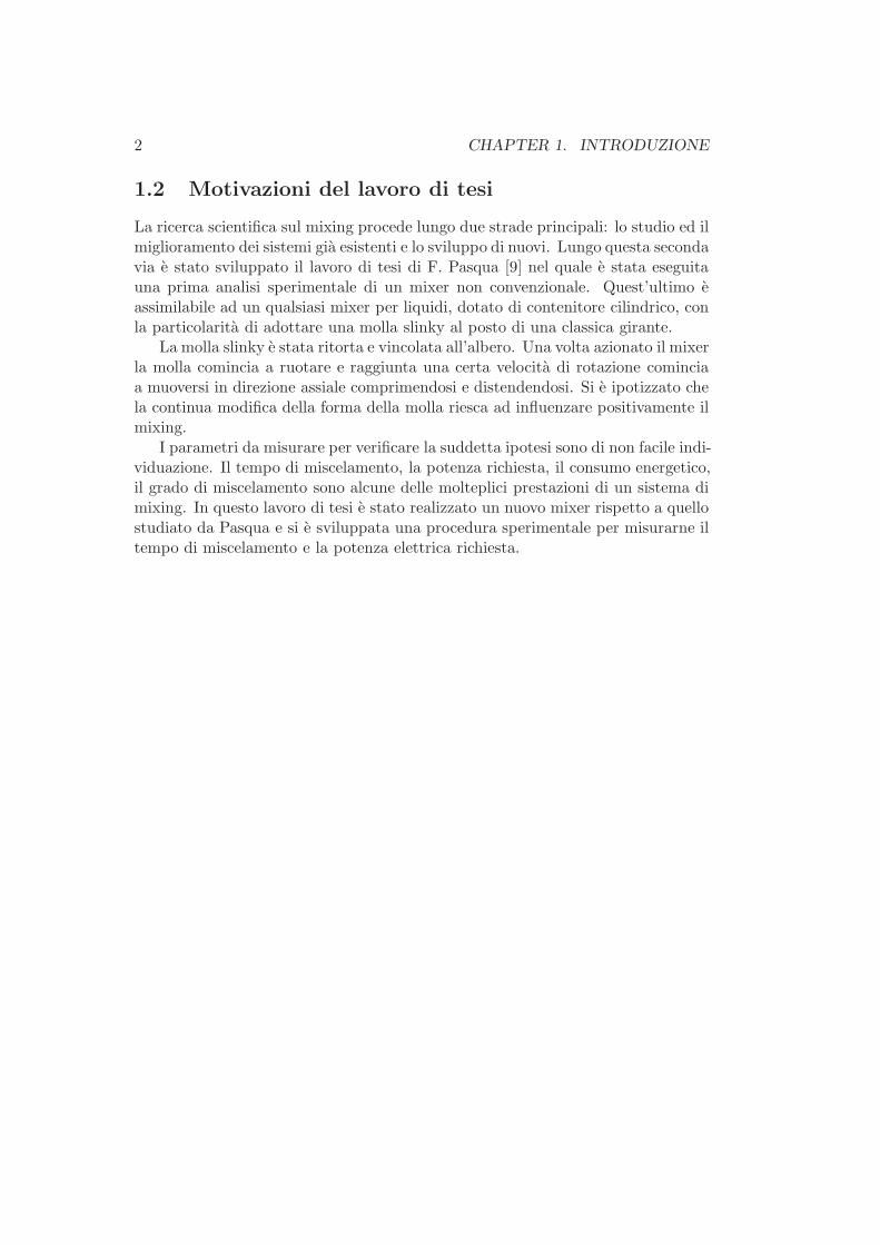
1.2 Motivazioni del lavoro di tesi

La ricerca scientifica sul mixing procede lungo due strade principali: lo studio ed ilmiglioramento dei sistemi gia esistenti e lo sviluppo di nuovi. Lungo questa secondavia e stato sviluppato il lavoro di tesi di F. Pasqua [9] nel quale e stata eseguitauna prima analisi sperimentale di un mixer non convenzionale. Quest’ultimo eassimilabile ad un qualsiasi mixer per liquidi, dotato di contenitore cilindrico, conla particolarita di adottare una molla slinky al posto di una classica girante.

La molla slinky e stata ritorta e vincolata all’albero. Una volta azionato il mixerla molla comincia a ruotare e raggiunta una certa velocita di rotazione cominciaa muoversi in direzione assiale comprimendosi e distendendosi. Si e ipotizzato chela continua modifica della forma della molla riesca ad influenzare positivamente ilmixing.

I parametri da misurare per verificare la suddetta ipotesi sono di non facile indi-viduazione. Il tempo di miscelamento, la potenza richiesta, il consumo energetico,il grado di miscelamento sono alcune delle molteplici prestazioni di un sistema dimixing. In questo lavoro di tesi e stato realizzato un nuovo mixer rispetto a quellostudiato da Pasqua e si e sviluppata una procedura sperimentale per misurarne iltempo di miscelamento e la potenza elettrica richiesta.

Chapter 2

Percorso di ricerca

Lo scopo di questo lavoro di tesi e di effettuare delle misure sul mixing turbolentoper qualificare le caratteristiche di un mixer non convenzionale nel quale vieneusata una molla slinky come elemento rotante. Esistono svariati elementi perqualificare un sistema di mixing: il tempo di miscelamento, il consumo energetico,il consumo di potenza e cosı via. Il primo obiettivo del lavoro e stata la scelta deltipo di dati da misurare. Sono stati scelti il tempo di miscelamento ed il consumodi potenza. Oltre a tre configurazioni con la molla, ne abbiamo studiata ancheuna piu classica utilizzando un’elica.

Non e possibile parlare di tempo di miscelamento in termini assoluti poiche vacalcolato in funzione del grado di omogeneita che si vuole ottenere. Tipicamente siricerca il tempo necessario per ottenere un’omogeneizzazione al 95% cioe l’istantedi tempo oltre il quale la misura rimane tra il 95% ed il 105% del valore finale. Ilvalore attribuito al grado desiderato risulta essere funzione del tipo di impiego chesi sta facendo del mixer.

Esistono diversi tipi di prove: basate sulla lettura di sensori oppure su metodi divisualizzazione. In questo lavoro abbiamo effettuato delle prove basate su misure ditemperatura. Variando la temperatura nel mixer ed azionandolo si puo ottenere iltempo di miscelamento analizzando i dati acquisiti. Abbiamo dotato il setup di unnumero elevato di termocoppie per poter avere informazioni lungo tutta l’altezzadel cilindro. Per variare la temperatura si e previsto un sistema di raffreddamentodel fondo tramite un bagno termostatato.

L’altro parametro che abbiamo deciso di misurare e la potenza elettrica con-sumata. Questo dato e facilmente calcolabile poiche e il prodotto tra corrente etensione di alimentazione del motore. La tensione e nota in quanto regolata sull’a-limentatore. Per misurare la corrente ci siamo serviti di un sensore. Ovviamente,ponendoci a questo livello, il consumo non e esattamente quello necessario al solomixing ma risulta maggiorato da contributi esterni.

Per validare la scelta di raffreddare il fondo si e studiata la soluzione analiti-ca per lo scambio termico in un corpo bidimensionale semi-infinito. Tale teoriapermette di calcolare la distribuzione nello spazio e l’andamento nel tempo dellatemperatura in un corpo di estensione semi-infinita a contatto con una parete al-

3

4 CHAPTER 2. PERCORSO DI RICERCA

la temperatura Tw. Gia da queste prime prove teoriche si e capito che l’idea diraffreddare il fondo, pur evitando moti convettivi nell’acqua, avrebbe comportatonotevoli svantaggi in termini di tempo.

Abbiamo modellato il mixer mediante il software SolidWork. Il setup progetta-to e costituito dal mixer, da un sistema di alimentazione, da ventisette termocoppie,da un encoder, da un sensore di corrente, da un sistema di acquisizione dati1 e dauna copertura in materiale isolante2.

Il sistema durante le prove acquisisce le termocoppie a 3Hz per l’intera duratadella prova. I dati relativi al motore, cioe corrente ed encoder, vengono acquisiti a1KHz. Per evitare che i file contenenti i dati acquisiti dal motore siano eccessiva-mente grandi la loro acquisizione avviene nei primi istanti di tempo e dopo il suoavvio. In tutta la fase intermedia non viene acquisito alcun dato. Il salvataggiodegli istanti iniziali e essenziale per riuscire a ricavare il momento in cui vieneacceso il motore. Questo istante viene considerato come inizio del mixing.

Si e eseguita una prova di stratificazione totale dell’acqua registrando un temposuperiore alla decina di ore. Si e poi azionato il mixer individuando un tempo dimiscelamento di poche decine di secondi. Dovendo testare il mixer per moltecondizioni differenti si e pensato di modificare il sistema in modo da permetteredei tempi di realizzazione prove piu brevi. Con la stratificazione avremmo avutoil vantaggio di poter imporre facilmente le condizioni iniziali di ogni test pagandolo scotto di prove molto lunghe. Abbiamo quindi implementato un sistema diriscaldamento3 da porre al di sotto del tappo del mixer. In questo modo siamostati in grado di far variare in poco tempo ed in modo sostanziale la temperaturadell’acqua per sola conduzione. Si e subito notato che riscaldando il sistema, sipotevano ottenere rapidi cambiamenti degli strati superiori gia dopo pochi minuti.Si e ipotizzato che a differenza del sistema di raffreddamento, con il riscaldamentosi possano raggiungere differenze di temperatura, tra parete e acqua, molto grandi.Per completezza si e studiato il caso del riscaldamento sfruttando la soluzioneanalitica.

Si e quindi iniziato un processo iterativo per individuare il metodo per calcolareil tempo di miscelamento e la procedura da attuare per avere prove con le mede-sime condizioni di pre-mixing. Dopo svariati test abbiamo individuato le seguentiprocedure.

In quella numerica per la misura del tempo di miscelamento abbiamo analiz-zato la derivata delle temperature, calcolata tramite differenze finite. La derivatadi tutte le temperature risulta molto piccola ma ha delle importanti variazioni nel-l’intervallo di tempo in cui avviene il miscelamento. Una volta individuato il suomassimo, in valore assoluto, muovendosi in avanti sull’asse dei tempi si e cercatol’istante nel quale il massimo della deviazione standard diventava minore di 0.0005,valore corrispondente ad un grado di omogeneita di circa il 98%.

1schede della NI e un computer con LabVIEW2removibile3costituito da una resistenza

5

Abbiamo definito la STD come:

σi(t) =

(

Ti(t)− (T fi − T f

a )

Ta(t)− 1

)2

(2.1)

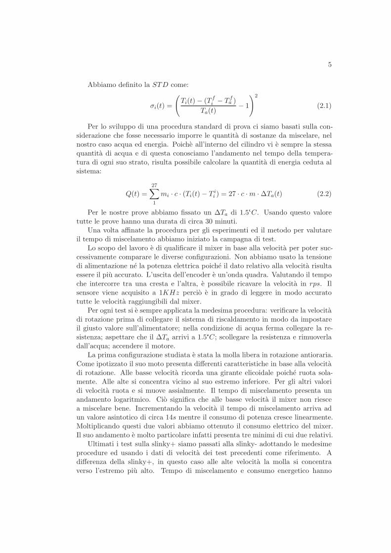
Per lo sviluppo di una procedura standard di prova ci siamo basati sulla con-siderazione che fosse necessario imporre le quantita di sostanze da miscelare, nelnostro caso acqua ed energia. Poiche all’interno del cilindro vi e sempre la stessaquantita di acqua e di questa conosciamo l’andamento nel tempo della tempera-tura di ogni suo strato, risulta possibile calcolare la quantita di energia ceduta alsistema:

Q(t) =

27∑

1

mi · c · (Ti(t)− T ii ) = 27 · c ·m ·∆Ta(t) (2.2)

Per le nostre prove abbiamo fissato un ∆Ta di 1.5°C. Usando questo valoretutte le prove hanno una durata di circa 30 minuti.

Una volta affinate la procedura per gli esperimenti ed il metodo per valutareil tempo di miscelamento abbiamo iniziato la campagna di test.

Lo scopo del lavoro e di qualificare il mixer in base alla velocita per poter suc-cessivamente comparare le diverse configurazioni. Non abbiamo usato la tensionedi alimentazione ne la potenza elettrica poiche il dato relativo alla velocita risultaessere il piu accurato. L’uscita dell’encoder e un’onda quadra. Valutando il tempoche intercorre tra una cresta e l’altra, e possibile ricavare la velocita in rps. Ilsensore viene acquisito a 1KHz percio e in grado di leggere in modo accuratotutte le velocita raggiungibili dal mixer.

Per ogni test si e sempre applicata la medesima procedura: verificare la velocitadi rotazione prima di collegare il sistema di riscaldamento in modo da impostareil giusto valore sull’alimentatore; nella condizione di acqua ferma collegare la re-sistenza; aspettare che il ∆Ta arrivi a 1.5°C; scollegare la resistenza e rimuoverladall’acqua; accendere il motore.

La prima configurazione studiata e stata la molla libera in rotazione antioraria.Come ipotizzato il suo moto presenta differenti caratteristiche in base alla velocitadi rotazione. Alle basse velocita ricorda una girante elicoidale poiche ruota sola-mente. Alle alte si concentra vicino al suo estremo inferiore. Per gli altri valoridi velocita ruota e si muove assialmente. Il tempo di miscelamento presenta unandamento logaritmico. Cio significa che alle basse velocita il mixer non riescea miscelare bene. Incrementando la velocita il tempo di miscelamento arriva adun valore asintotico di circa 14s mentre il consumo di potenza cresce linearmente.Moltiplicando questi due valori abbiamo ottenuto il consumo elettrico del mixer.Il suo andamento e molto particolare infatti presenta tre minimi di cui due relativi.

Ultimati i test sulla slinky+ siamo passati alla slinky- adottando le medesimeprocedure ed usando i dati di velocita dei test precedenti come riferimento. Adifferenza della slinky+, in questo caso alle alte velocita la molla si concentraverso l’estremo piu alto. Tempo di miscelamento e consumo energetico hanno

6 CHAPTER 2. PERCORSO DI RICERCA

andamento simile alla configurazione precedente. Il consumo energetico ha ancoratre minimi ma molto ravvicinati tra loro.

Finiti i test con la molla libera, la abbiamo vincolata all’albero in modo daimpedire qualsiasi movimento in direzione assiale. Con questa configurazione ilmixer assomiglia molto di piu ad alcuni mixer gia esistenti. A differenza delle con-figurazioni precedenti si riscontra un peggioramento delle caratteristiche generalidel mixer.

Come configurazione classica di confronto e stata presa una girante assiale. Iltempo di miscelamento ha anche per questa configurazione un andamento loga-ritmico. Il consumo di potenza non e piu lineare ma esponenziale rispetto allavelocita, probabilmente a causa della resistenza idrodinamica. Anche il consumoenergetico cresce esponenzialmente con la velocita.

Confrontando le diverse configurazioni del mixer e possibile trarre alcuni im-portanti considerazioni. In termini energetici la molla vincolata consuma piu deicasi in cui e libera di muoversi assialmente. Cio e dovuto ai maggiori tempi dimiscelamento ed al maggior consumo di potenza elettrica. Comparando poi le treconfigurazioni slinky con la girante, quest’ultima risulta piu efficace ed efficientealle basse velocita. Alle alte essa rimane efficace, in termini di tempo, ma risultamolto meno efficiente.

I risultati ottenuti sono stati molto soddisfacenti e presagiscono la possibilitadi uno studio piu approfondito di questo tipo di mixer. Interessante e il datorelativo al consumo di potenza elettrica il quale potrebbe suggerire un minoredanneggiamento meccanico del fluido. Occorrera quindi cercare di comprenderemeglio le dinamiche all’interno del mixer.

Chapter 3

Introduction

3.1 The importance of mixing

Mixing, as a discipline, is currently seeing a growing interest by many scientificand industrial sectors. This is a complex phenomenon but the potential benefitsof a better understanding are pushing research.

Mixing plays a key role in of most of the industrial production systems such aschemical, pharmaceutical or food and it is very important in other specific fieldssuch as in medical equipments or in biotechnology.

Whether it is mixing of two or more liquids, liquids and solids, gases and liq-uids the quality and the properties of the products obtained depend on the mixingprocess. Although there are many industrial operations in which mixing require-ments are readily scaled-up from known correlations, many operations require amore careful evaluation. The cost of a targeted development is smaller than thecost of adapting a system developed inaccurately and has great economic potential.Numerous studies demonstrated that losses due to poor-mixing can be huge. In1989, the cost of poor mixing was estimated at $1 billion to $10 billion only in theU.S. chemical industry [3].

The wide variety and ever increasing complexity of mixing processes encoun-tered in industrial applications requires careful selection, design and scale up toensure effective and efficient mixing. Today’s competitive production systems needrobust equipment that has to be capable of faster blend times, lower power con-sumption and adaptability for use with multiple products. A mixer is no longer ageneric production tool, but a critical and decisive business tool.

3.2 Reasons of the research work

Scientific research on mixing proceeds along two main paths: study and improve-ment of existing systems and development new ones. Following this second paththe thesis work of F. Pasqua[9] has been developed. In this work was made a firstexperimental analysis of an unconventional mixer. This mixer had a cylindrical

7

8 CHAPTER 3. INTRODUCTION

container as any other mixer for liquids but it used a slinky spring instead of aclassical impeller.

The spring is twisted and fixed to the rotational shaft. During rotation it isfree to move axially compressing and relaxing. It has been speculated that thecontinuous change in its shape is able to positively influence the mixing.

It is not easy to find the parameters needed to prove this hypothesis. Mixingtime, electric power consumption, energy consumption, degree of mixing are someof the many characteristics of this complex system. In this thesis we created a newmixer 1 and we developed an experimental procedure to measure mixing time andelectrical power consumption.

3.3 Thesis structure

The outline of the thesis is as follows. In Chapter 3 we introduce the research areaand the aim of this work. In Chapter 4 we review the preliminary studies thatpreceded the design of the experimental setup. In Chapter 5 we describe the exper-imental setup starting from the design to the acquisition system. Chapter 6 showsall the tests made to validate the experimental setup including the estimation oferrors. In Chapter 7 we present the experimental data of the work. First eachconfiguration and then the comparison between all of them. Chapter 8 containsthe conclusions of this research and shows the possible future developments.

1new compared to the one studied by Pasqua

Chapter 4

Preliminary studies

4.1 Mixing

We define mixing a physical process which aims at reducing inhomogeneity influids to achieve a desired process result by eliminating gradients of concentration,temperature, and other properties. Liquid mixing and other mixing operationsconcerning a dispersed phase in a liquid are a common processes in the chemicaland pharmaceutical manufacturing industry. These operations are usually carriedout in glass-lined, stirred, torispherical-bottomed reactors.

4.1.1 Mixer for liquids

Mixers for liquids can, usually, be classified according to the viscosity of the sub-stances which need to be mixed (fig. 4.1)[8]. Mixing impellers are designed toproduce turbulence and pump fluid. For mixing both of these elements are essen-tial. They produce fluid shear and fluid velocity respectively. It is necessary thatthe fluid agitated by the impeller sweeps the entire tank in a sensible time and besufficient to reach the most remote parts of the vessel. Fluid velocity also preventssolids sedimentation and produces flow over heating or cooling coils when necessary.Fluid shear means turbulent eddies. These are essential to micro-mixing. Mixingis certain to be inefficient unless flow in tank is turbulent. A good mixing couldbe described as a combination of three physical process : distribution, dispersionand diffusion. Distribution is dispersion of materials caused by bulk motion. It is often the

slowest step in mixing process. Dispersion is the act of spreading out. Dispersion breaks up bulk flow intosmaller and smaller eddies. Turbulent diffusion is dispersion in turbulent flows caused by the motions ofeddies. Molecular diffusion is diffusion caused by relative molecular motion.

9

10 CHAPTER 4. PRELIMINARY STUDIES

Figure 4.1: Viscosity ranges for different impellers

Distribution, dispersion and diffusion are related to different scales of mixing:macromixing, mesomixing and micromixing. The first is the slowest step. The lastis the fastest.

All mixing impellers produce both fluid velocity and fluid shear, but differenttypes of impellers produce different degrees of flow and turbulence, either of whichmay be important, depending on the application.

The choice of a mixer for a particular application depends on numerous processfactors, some of which are: Type of application Viscosity Tank geometry Retention time and/or blend time

In this thesis we mixed only water so we focused on mixers equipped withpropellers or turbines. Mixing impellers can be divided into two generals categories:radial flow or axial flow. These two configurations generate different flow fields(fig. 4.2).

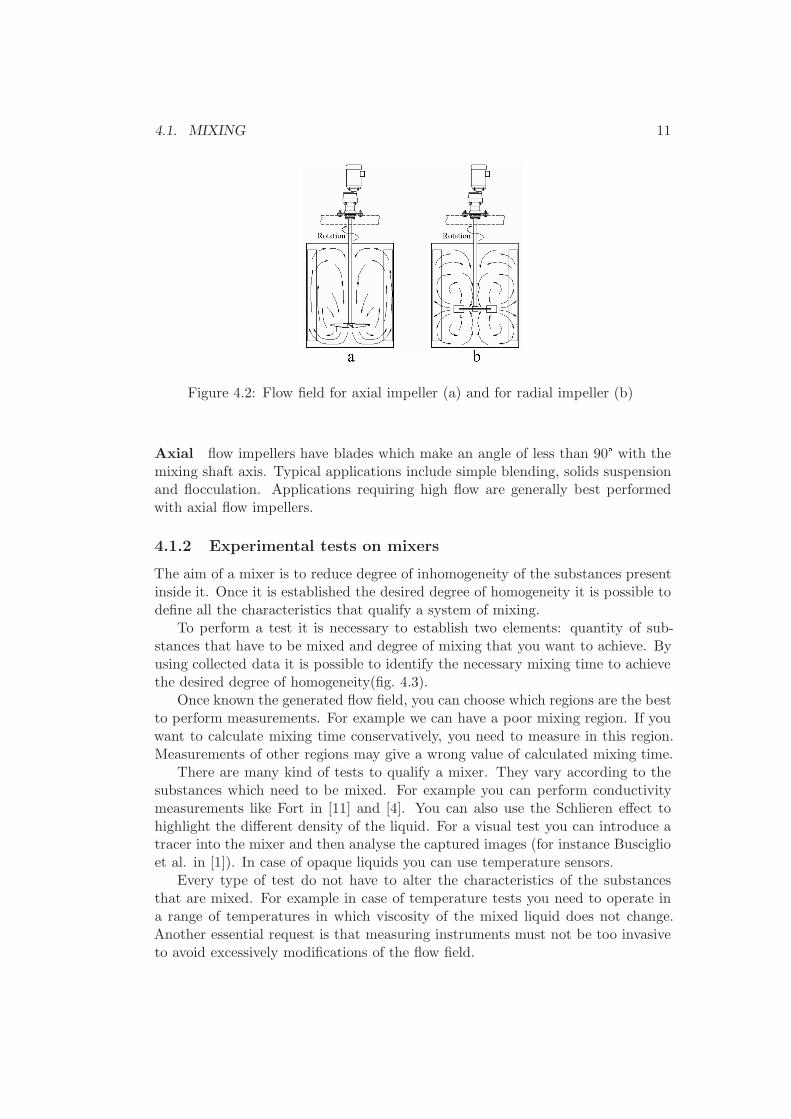
Radial flow impellers have multiple flat blades that are mounted parallel tothe axis of the mixing shaft. Typical uses of these instruments are gas/liquiddispersion, liquid/liquid dispersion, flash mixing and low level mixing applications.If high shear is required, radial flow impellers should be preferred.

4.1. MIXING 11

Figure 4.2: Flow field for axial impeller (a) and for radial impeller (b)

Axial flow impellers have blades which make an angle of less than 90° with themixing shaft axis. Typical applications include simple blending, solids suspensionand flocculation. Applications requiring high flow are generally best performedwith axial flow impellers.

4.1.2 Experimental tests on mixers

The aim of a mixer is to reduce degree of inhomogeneity of the substances presentinside it. Once it is established the desired degree of homogeneity it is possible todefine all the characteristics that qualify a system of mixing.

To perform a test it is necessary to establish two elements: quantity of sub-stances that have to be mixed and degree of mixing that you want to achieve. Byusing collected data it is possible to identify the necessary mixing time to achievethe desired degree of homogeneity(fig. 4.3).

Once known the generated flow field, you can choose which regions are the bestto perform measurements. For example we can have a poor mixing region. If youwant to calculate mixing time conservatively, you need to measure in this region.Measurements of other regions may give a wrong value of calculated mixing time.

There are many kind of tests to qualify a mixer. They vary according to thesubstances which need to be mixed. For example you can perform conductivitymeasurements like Fort in [11] and [4]. You can also use the Schlieren effect tohighlight the different density of the liquid. For a visual test you can introduce atracer into the mixer and then analyse the captured images (for instance Busciglioet al. in [1]). In case of opaque liquids you can use temperature sensors.

Every type of test do not have to alter the characteristics of the substancesthat are mixed. For example in case of temperature tests you need to operate ina range of temperatures in which viscosity of the mixed liquid does not change.Another essential request is that measuring instruments must not be too invasiveto avoid excessively modifications of the flow field.


Figure 4.3: Example of homogenization

Processing mixing time data

Data collected by the conductivity (Fort in [11]), thermocouple or pH techniquesmust be processed to obtain mixing time for the system that is under investigation.Data must be first normalized to eliminate the effect of different probe gains. Dataare normalized between an initial value of zero that is measured before addingtracer, and a final stable value measured after test is completed. The normalizedoutput is obtain by

C ′

i =Ci − C0

C∞ − C0

(4.1)

where C ′

i is normalized probe output. Mixing time is defined as time that normal-ized probe output needs to reach and remain between 95 and 105% (±5%) of thefinal equilibrium value.

4.1.3 Dimensionless numbers

To compare different mixers is useful to define some dimensionless numbers. Formixing tanks the Reynolds number is defined as

Re =ρND2

µ(4.2)

where ρ is the fluid density, D is the impeller diameter, N is the impeller speed(in rps) and µ is the dynamic viscosity.

The power number is a dimensionless parameter that provides a measure ofthe power requirements for the operation of an impeller. It is defined a

Np =P

ρN3D5(4.3)

Another number is the dimensionless mixing time that is defined as

Nt = N ∗ tm (4.4)

4.1. MIXING 13

Nt can be considered as the number of complete rounds of the impeller to reachthe desired value of homogeneity.

With our mixer we can use only the definition of dimensionless mixing timebecause of the impossibility to set a value of D for the slinky.


4.2 Theory of heat transfer in semi-infinite plane

We used [6] as reference. We have a bi-dimensional semi-infinite region. Oneboundary, initially at T = T0, is suddenly cooled (or heated) at a new temperature,T∞.

General functions that we are going to use can be considered valid in absenceof convective movements.

Fourier’s law of heat conduction

∂2T

∂x2=

ρc

λ

∂T

∂t(4.5)

α =λ

ρc(4.6)

∂2T

∂x2=

1

α

∂T

∂t(4.7)

This is a second order PDE. We need to change it in an ODE in order tofind an analytical solution. We introduce a new variable and make temperaturedimensionless using Θ.

ξ =x

√αt

(4.8)

∆T = T0 − Tw (4.9)

∂T

∂t= ∆T

∂Θ

∂t= ∆T

∂ξ

∂t

∂Θ

∂ξ= ∆T

(

−x

2t√αt

)

∂Θ

∂ξ(4.10)

We do the same thing with second derivative

∂T

∂x= ∆T

∂ξ

∂x

∂Θ

∂ξ=

∆T√αt

∂Θ

∂ξ(4.11)

∂2T

∂x2=

∂

∂x

(

∆T√αt

∂Θ

∂ξ

)

=∆T

αt

∂2Θ

∂ξ2(4.12)

By substituting the first and the last of these derivatives in heat conductionequation, we get

d2Θ

dξ2= −

ξ

2

dΘ

dξ(4.13)

Initial condition for previous equation is

T (t = 0) = Ti (4.14)

Θ(ξ → ∞) = 1 (4.15)

4.2. THEORY OF HEAT TRANSFER IN SEMI-INFINITE PLANE 15

and the one known boundary condition is

T (x = 0) = Tw (4.16)

Θ(ξ = 0) = 0 (4.17)

If we call dΘ/dξ ≡ χ we obtain an ODE

dχ

dξ= −

ξ

2χ (4.18)

which can be integrated once to get

χ ≡dΘ

dξ= C1e

−ξ2/4 (4.19)

and we integrate this a second time to get

Θ(ξ) = C1

∫ ξ

0

e−ξ2/4dξ +Θ(0) (4.20)

The b.c. is now satisfied and we need only substitute Θ(ξ) in the i.c. to solvefor C1:

1 = C1

∫ ξ

0

e−ξ2/4dξ (4.21)

The definite integral is given by integral tables as√π,so

C1 =1√π

(4.22)

Therefore solution to the problem of conduction in a semi-infinite region, sub-ject to a b.c. of the first kind is

Θ =1√π

∫ ξ

0

e−ξ2/4dξ =2√π

∫ ξ/2

0

e−s2ds ≡ erf(ξ/2) (4.23)

erf is called error function. We can calculate ξ/2 = for x during time. Thenwe can find Θ and the relative value of temperature.

In our tests T0 is the initial temperature of water that we assume be the sameas the ambience temperature. Tw is the temperature of the bottom of the cylinderthat we assume to be constant because of thermostatic bath.

We used this method for evaluate time needed to cool substantially water inthe mixer. In the graphs x-axis is the height of water in the cylinder.


0 0.5 1 1.5 2 2.5 3 3.5 40

0.2

0.4

0.6

0.8

1

ξ/2

Θ

Figure 4.4: Error function

0 0.05 0.1 0.15 0.2 0.25 0.3 0.35 0.40

5

10

15

20

25

30

h[m]

T[C

]

Figure 4.5: Theoretical temperature distribution in the cylinder at t=0

4.2. THEORY OF HEAT TRANSFER IN SEMI-INFINITE PLANE 17

0 0.05 0.1 0.15 0.2 0.25 0.3 0.35 0.40

5

10

15

20

25

30

h[m]

T[C

]

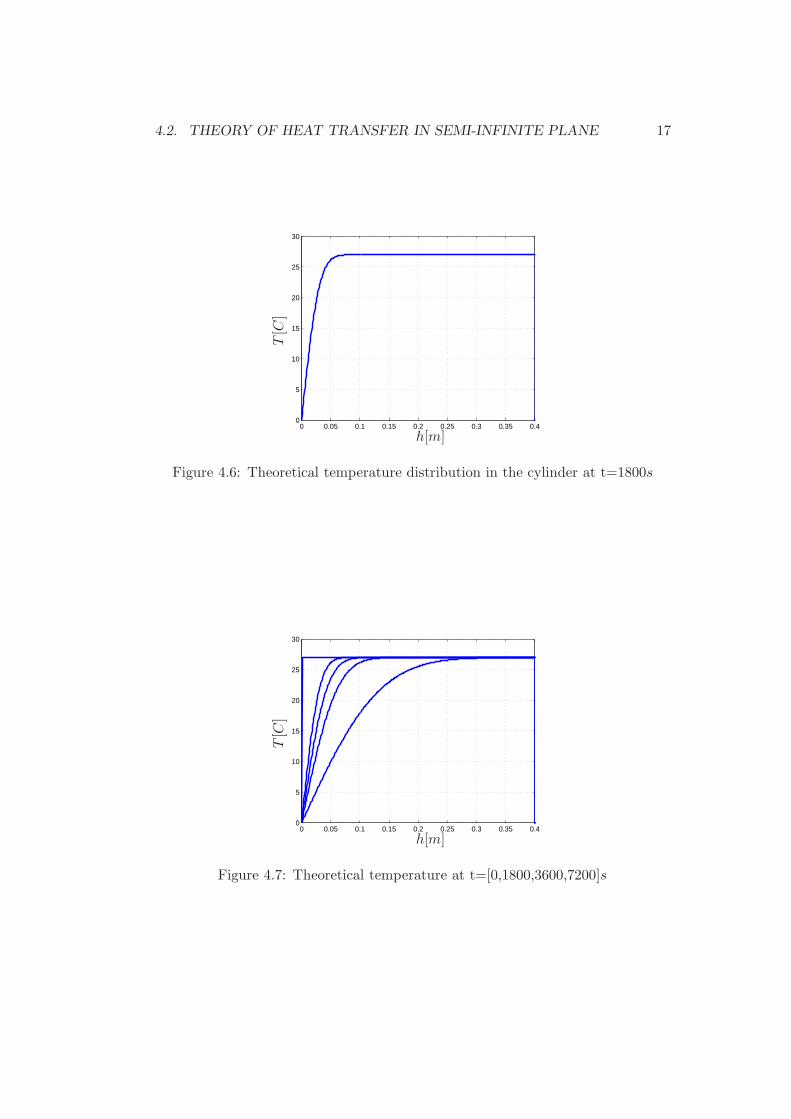
Figure 4.6: Theoretical temperature distribution in the cylinder at t=1800s

0 0.05 0.1 0.15 0.2 0.25 0.3 0.35 0.40

5

10

15

20

25

30

h[m]

T[C

]

Figure 4.7: Theoretical temperature at t=[0,1800,3600,7200]s

Chapter 5

Experimental Setup

5.1 Design choises

Designing the experimental setup was the first step of this research work. Wedecided to make tests using measures of temperature.

The first idea was to cool the bottom of the mixer, but after the first tests wedecided to improve the setup including a heating system in the top layer. Thissolution allowed us to heat or cool the water without convective movements. Weplaced 27 thermocouples to measure the temperature along the entire height of thecylinder. We used as many thermocouples as we could acquire because we want tohave the more accurate data as possible. We measured the average temperatureof the water inside the mixer and we calculated the amount of energy given orsubtracted from the system. In every test we exchange with the water the sameamount of energy. The thermocouples allowed us to identify the mixing time withMatlab.

We used an external power supply to power the motor to avoid problems ofelectric instability. We put a current sensor between the motor and the powersupply and we calculated the electric power consumption using the acquired dataof the current and the voltage.

The main aim of this work was to test the mixer using the rotational velocityof the mixer as reference. For this reason we used a motor equipped with encoderfor the highest accuracy possible.

The experimental setup changed during the preliminary tests. We improved itadding some useful elements: a tap to empty the cylinder, a hole in the cap to fillit and a covering of insulating material.

19

20 CHAPTER 5. EXPERIMENTAL SETUP

5.2 3D model

We used SolidWorks[2] to design the mixer. This program allowed us to be veryprecise in designing each part and it made faster the creating phase.

Figure 5.1: 3D model of the mixer

The main dimensions of the mixer are these:

internal cylinder diameter 14cmexternal cylinder diameter 15cmcylinder height 40cmshaft diameter 6mm

Initially we designed an external support for the motor but we found that thesetup was heavy enough to avoid excessive vibrations therefore we mounted themotor on top of the mixer.

Main components of the mixer: a slinky spring a plexiglass cylinder a cap of PVC an aluminum shaft a rigid joint

5.3. CONFIGURATIONS OF THE MIXER 21 an aluminum circular bottom two supports for the slinky a column of corial for the thermocouples a square aluminum base a base of corial for the heat exchanger some o’ring

5.3 Configurations of the mixer

We tested four different configurations of the mixer: free slinky+ that moves counter-clockwise free slinky- that moves clockwise fixed slinky that moves counter-clockwise impeller that moves counter-clockwise

The slinky used has a diameter of 3cm and 70 coils. We fixed one terminal at85mm from the bottom of the mixer then we twisted the slinky 2 times and fixedthe other terminal at 29cm from the bottom. We used a 120mm diameter impellerfixed it at 10cm from the bottom of the mixer.

Figure 5.2: Slinky spring mounted on the shaft


5.4 Power supply

Agilent E3631A The Agilent E3631A (fig. 5.3) is a high performance 80 watt-triple output programmable DC power supply. In our tests we usually used +25Voutput regulated by control knob. We could change the voltage very precisely witha minimum step of 0.01V . Using ”Output On/Off” button it was possible to setup the value of the output voltage and to turn the output on when needed.

Figure 5.3: Programmable DC power supply Agilent E3631A

Secondary power supply We used a non controlled secondary DC power sup-ply for the heating system. The output voltage of this power supply is 13V. Usinga resistor of 6Ω we created a 20W heating system.

5.5 Heating and cooling system

Cooling system Since the bottom of the mixer is an heat exchanger we useda thermostatic bath to cool it. Water enters in the base and exchanges heat withthe mixer aluminum bottom and then returns to the thermostatic bath.

Heating system We created a circular resistor of 6Ω and used some non-conductiveelements as a supporting structure. We attached it to a long screw with two nuts.This screw passes through the cap and we could change its height with anothernut.

5.6 Motor

During the preliminary tests we tried different motors. After several tests wedecided to use a Pololu Metal Gearmotor 37Dx52L mm (fig. 5.6).

5.6. MOTOR 23

Figure 5.4: Particular of the heat exchanger under the mixer

Figure 5.5: View of the heat exchanger under the mixer

Figure 5.6: Metal Gearmotor 37Dx52L mm


Gear Ratio 19:1Speed 12V 500rpmStall Torque 12V 84 oz-inStall Current 12V 5A

Table 5.1: Pololu motor characteristics

This motor has a very linear characteristic curve with no irregularities espe-cially at the low velocities.

5.7 Sensors

5.7.1 Thermocouples

We built our thermocouple using a thermocouple wire1 from TERSID.S.r.l. andmedical tip-less needles. We fixed the wire using industrial glue. Then we putthese sensors in drilled screws that were inserted in the holes of the cylinder.

Figure 5.7: View of thermocouples

We created 27 thermocouples with needles and 2 without them. We used thesetwo to measure ambient temperature and bottom heat exchanger temperature. Welinked all the thermocouples to the NI 9213 to acquire data.

5.7.2 Current sensor

We measured current using a ACS712 that has a Vcc of 5V and we linked it to theoutput voltage of the NI6009. We mounted it on the wire that links the motor tothe power supply. The output is a voltage but we used its data-sheet to calculatethe current.

1TEX-36-TT

5.7. SENSORS 25

Figure 5.8: Current sensor ACS712

5.7.3 Encoder

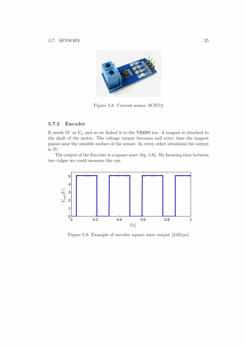
It needs 5V as Vcc and so we linked it to the NI6009 too. A magnet is attached tothe shaft of the motor. The voltage output becomes null every time the magnetpasses near the sensible surface of the sensor. In every other situations the outputis 5V .

The output of the Encoder is a square wave (fig. 5.9). By knowing time betweentwo ridges we could measure the rps.

0 0.2 0.4 0.6 0.8 10

1

2

3

4

5

t[s]

Vout[V]

Figure 5.9: Example of encoder square wave output [3.65rps]


5.8 Acquisition system

In each test we acquired this data: temperature of each thermocouples output voltage of the encoder motor current

5.8.1 LabVIEW

NI LabVIEW is a software for the design of systems that uses icons, terminals andconnections rather than text, so you can program the way you think. LabVIEWincludes tools based on advanced programming features for the development ofcontrol applications, measurement and analysis with professional user interfaces.We used it for acquiring data from two NI9213 and from NI9205. We createda custom interface which allowed us to see the value of all thermocouples andencoder output (fig. 5.10).

Figure 5.10: Screenshot of LabVIEW virtual instrument

When a test starts the system saves the value of the average temperatureand every time it calculates its variation. You can choose a value of averagetemperature maximum increase. When average temperature reaches this value

5.8. ACQUISITION SYSTEM 27

LabVIEW make an alert sound. During all the test LabVIEW saves temperaturesdata. The motor data are saved only at the initial time and when the heatingphase is over. The thermocouples data are acquired at a rate of 3Hz while themotor data are acquired at 1KHz [5].

5.8.2 NI USB-6009

NI USB-6009 provides basic data acquisition functionality for applications, datalogging, portable measurements and laboratory experiments. These cards have anaccessible cost to students and offer adequate performance for more sophisticatedmeasurement applications.

Figure 5.11: Low-Cost Multifunction DAQ NI USB-6009

We used it to power encoder and current sensor.

5.8.3 NI9213 and NI9205

The NI9213 is a high-density thermocouple module for NI C Series carriersdesigned for higher-channel-count systems. With this module, you can add ther-mocouples to mixed-signal test systems without taking up too many slots. Built-incold-junction compensation is the main feature of this device.

We used two of this device to acquire all the temperatures of the thermocouples.

The NI9205 is a C Series module, for use with NI CompactDAQ and Com-pactRIO chassis. The NI9205 features 32 single-ended or 16 differential analoginputs, 16-bit resolution, and a maximum sampling rate of 250 kS/s.

We used this device to acquire current sensor and encoder outputs.


Figure 5.12: Thermocouple Input Module NI9213

Figure 5.13: Voltage Input Module NI9205

5.9. MATLAB 29

5.9 Matlab

We used Matlab to post-process the acquired data. We divided the post-processin two main parts: one for the temperature data and one for the motor data.

5.9.1 Post-process of temperature data

These are the functions created for the temperature data: loadifle.m it opens the data file and saves the time in a vector and thetemperatures of all the thermocouples in a matrix smooth.m it smooths the data by applying a moving average of N points mixing.m it calculates the derivative of the temperatures to find where themixing is. It finds the maximum of the derivative and then moves forwardto find where the STD became littler than 0.0005 that mean an homogeneityof 97.75%. calibration.m it calculates the difference between the final average tempe-rature of each thermocouple and the total average temperature energy.m it calculates the average temperature graph.m it makes graph of the total test (fig. 5.14) graphmixing.m it makes graph of the interval of mixing (fig. 5.15)

0 500 1000 1500 200020

25

30

35

40

45

t[s]

T[C

]

Figure 5.14: Example of total graph of a test [3.65rps]


1535 1540 1545 1550 1555 1560 1565 1570

24

26

28

30

32

34

36

38

40

42

tmixing=22.33

t[s]

T[C

]

Figure 5.15: Example of mixing graph of a test [3.65rps]

5.9.2 Post-process of motor data

The motor data were saved in two different files: one for the encoder and one forthe current sensor.

We took the data in different times. We took the encoder data during the maintests. The current data were taken after them. Initially we measured current byacquiring voltage of a 1Ω resistor in series with the motor but we discovered thatmeasures were wrong. After all tests we calibrated the motor for every configura-tion and at every velocity (fig. 5.18).

We used the original current data to identify the start of the mixing in eachtest and to correct the value identified by studying the STD. In figure 5.17 youcan see that the current is null until 1596s. After this value it becomes biggerbecause LabVIEW is acquiring the current but the power supply is off so there isonly electrical noise. At 1635s we turned on the motor.

5.9. MATLAB 31

0 500 1000 1500 2000

0

0.5

1

t[s]

curren

t[A]

Figure 5.16: Example of original current data of a test [3.65rps]

1595 1600 1605 1610 1615 1620 1625 1630 1635

−4

−2

0

2

4

6

x 10−3

t[s]

curren

t[A]

Figure 5.17: Example of locating the beginning of the mixing [3.65rps]

0 2 4 6 8 100

1

2

3

4

5

rps[1/s]

pow

er[W

]

Figure 5.18: Example of power on rps graph


5.10 Experimental Procedure

This is the experimental procedure of each test2:

1. turn on the motor and set the required speed

2. disconnect the motor

3. wait until the water stops

4. start the program data acquisition on LabVIEW

5. turn on the resistor

6. wait until the average temperature increases of 1.5° C7. turn off the resistor

8. remove the resistor from water and block it

9. reconnect the motor

10. wait until the temperatures becomes stable

11. post-process acquired data.

2Before every set of test we filled the mixer with water until the height of the first thermocouple.At the end of daily tests we emptied it.

5.11. DIAGRAM OF THE EXPERIMENTAL SETUP 33

5.11 Diagram of the experimental setup

Figure 5.19: Diagram of the experimental setup

Chapter 6

Validation

6.1 Test of the thermocouples

Impermeability test We inserted every thermocouple produced in a little pipelinked to a syringe full of water to test their impermeability. The resulting waterlosses are minimal.

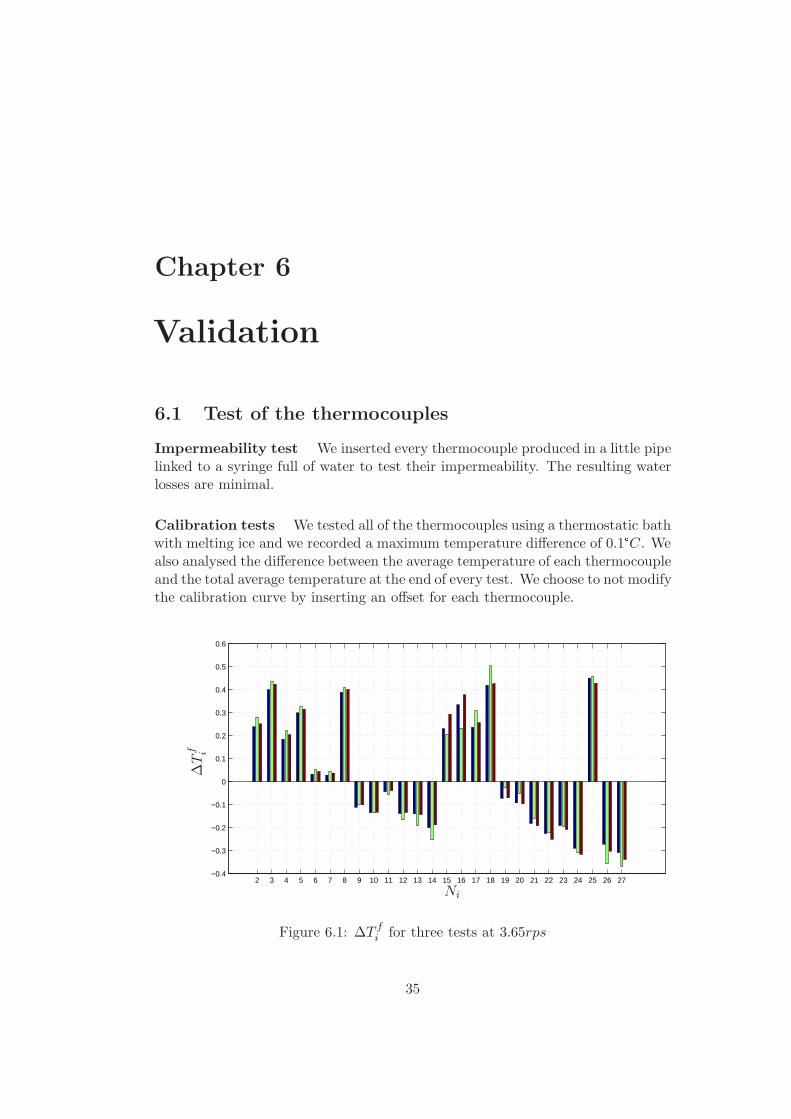
Calibration tests We tested all of the thermocouples using a thermostatic bathwith melting ice and we recorded a maximum temperature difference of 0.1°C. Wealso analysed the difference between the average temperature of each thermocoupleand the total average temperature at the end of every test. We choose to not modifythe calibration curve by inserting an offset for each thermocouple.

2 3 4 5 6 7 8 9 10 11 12 13 14 15 16 17 18 19 20 21 22 23 24 25 26 27−0.4

−0.3

−0.2

−0.1

0

0.1

0.2

0.3

0.4

0.5

0.6

Ni

∆Tf i

Figure 6.1: ∆T fi for three tests at 3.65rps

35

36 CHAPTER 6. VALIDATION

2 3 4 5 6 7 8 9 10 11 12 13 14 15 16 17 18 19 20 21 22 23 24 25 26 270

0.02

0.04

0.06

0.08

0.1

0.12

0.14

0.16

Ni

max

∆Tf i

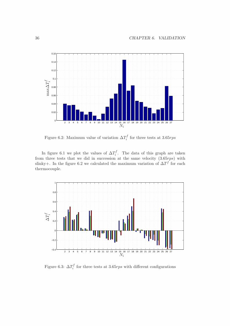
Figure 6.2: Maximum value of variation ∆T fi for three tests at 3.65rps

In figure 6.1 we plot the values of ∆T fi . The data of this graph are taken

from three tests that we did in succession at the same velocity (3.65rps) withslinky+. In the figure 6.2 we calculated the maximum variation of ∆T f for eachthermocouple.

2 3 4 5 6 7 8 9 10 11 12 13 14 15 16 17 18 19 20 21 22 23 24 25 26 27−0.4

−0.2

0

0.2

0.4

0.6

0.8

1

Ni

∆Tf i

Figure 6.3: ∆T fi for three tests at 3.65rps with different configurations

6.1. TEST OF THE THERMOCOUPLES 37

2 3 4 5 6 7 8 9 10 11 12 13 14 15 16 17 18 19 20 21 22 23 24 25 26 270

0.05

0.1

0.15

0.2

0.25

0.3

0.35

Ni

max

∆Tf i

Figure 6.4: Maximum value of variation ∆T fi for three tests at 3.65rps with dif-

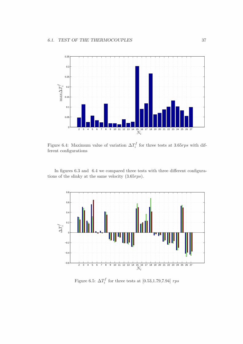
ferent configurations

In figures 6.3 and 6.4 we compared three tests with three different configura-tions of the slinky at the same velocity (3.65rps).

2 3 4 5 6 7 8 9 10 11 12 13 14 15 16 17 18 19 20 21 22 23 24 25 26 27−0.6

−0.4

−0.2

0

0.2

0.4

0.6

0.8

Ni

∆Tf i

Figure 6.5: ∆T fi for three tests at [0.53,1.79,7.94] rps


2 3 4 5 6 7 8 9 10 11 12 13 14 15 16 17 18 19 20 21 22 23 24 25 26 270

0.05

0.1

0.15

0.2

0.25

0.3

0.35

Ni

max

∆Tf i

Figure 6.6: Maximum value of variation ∆T fi for three tests at [0.53,1.79,7.94] rps

In figures 6.5 and 6.6 we compared three tests1 with three different velocities2

made in three different days.

2 3 4 5 6 7 8 9 10 11 12 13 14 15 16 17 18 19 20 21 22 23 24 25 26 27−0.4

−0.2

0

0.2

0.4

0.6

0.8

1

Ni

∆Tf i

Figure 6.7: ∆T fi for three tests at different velocities with different configurations

1slinky+2[0.53,1.79,7.94]rps

6.1. TEST OF THE THERMOCOUPLES 39

2 3 4 5 6 7 8 9 10 11 12 13 14 15 16 17 18 19 20 21 22 23 24 25 26 270

0.1

0.2

0.3

0.4

0.5

0.6

0.7

Ni

max

∆Tf i

Figure 6.8: Maximum value of variation ∆T fi for three tests at different velocities

with different configurations

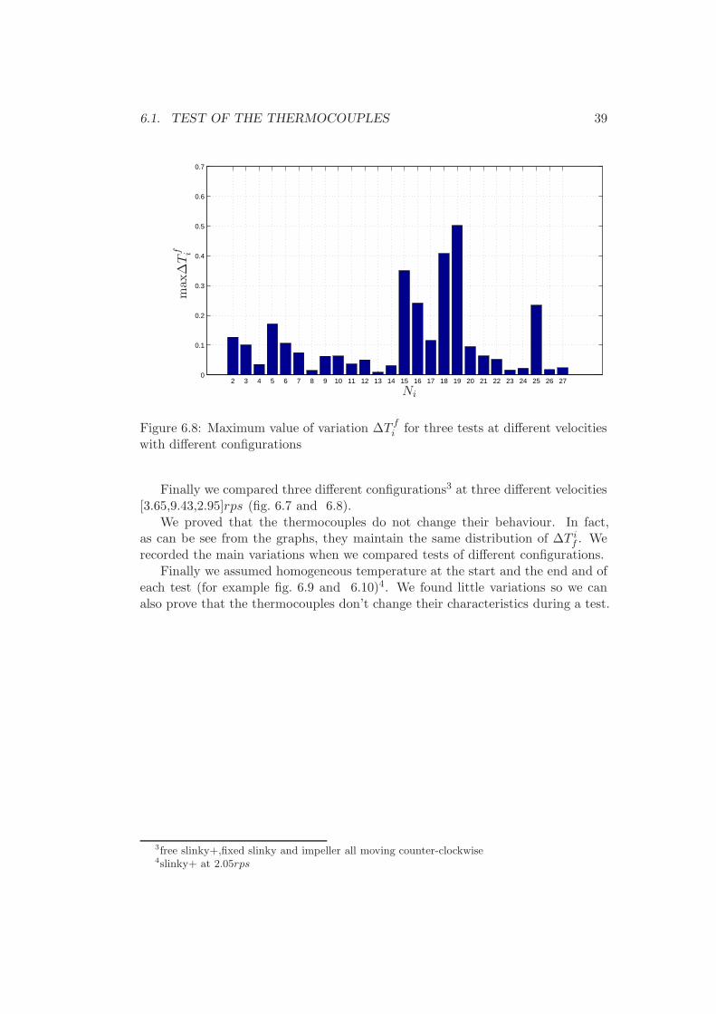
Finally we compared three different configurations3 at three different velocities[3.65,9.43,2.95]rps (fig. 6.7 and 6.8).

We proved that the thermocouples do not change their behaviour. In fact,as can be see from the graphs, they maintain the same distribution of ∆T i

f . Werecorded the main variations when we compared tests of different configurations.

Finally we assumed homogeneous temperature at the start and the end and ofeach test (for example fig. 6.9 and 6.10)4. We found little variations so we canalso prove that the thermocouples don’t change their characteristics during a test.

3free slinky+,fixed slinky and impeller all moving counter-clockwise4slinky+ at 2.05rps


2 3 4 5 6 7 8 9 10 11 12 13 14 15 16 17 18 19 20 21 22 23 24 25 26 27−0.5

0

0.5

1

Ni

∆Tf i

Figure 6.9: ∆T toti between T i

a and T fa

2 3 4 5 6 7 8 9 10 11 12 13 14 15 16 17 18 19 20 21 22 23 24 25 26 270

0.01

0.02

0.03

0.04

0.05

0.06

0.07

0.08

0.09

0.1

Ni

max

∆Tf i

Figure 6.10: Maximum value of variation ∆T toti between T i

a and T fa

6.2. COOLING TEST 41

6.2 Cooling test

Initially we decided to make tests using the thermostatic bath to cool down thebottom of the cylinder. The main idea was to let the water stratify and then turnon the mixer. We filled the cylinder and then we set the bath at a temperatureof 5°C. We left the setup work through the night5. The day after the water wastotally stratified (fig. 6.11). The found data were consistent with the theory ofheat transfer in semi-infinite plane (fig. 6.12)6.

0 1 2 3 4 5 6

x 104

8

10

12

14

16

18

20

22

24

t[s]

T[C

]

Figure 6.11: Stratification of the water with the cooling system

We tried to understand how much time is necessary to have a substantialchange of temperature in the cylinder. We have estimated that it takes aboutthree hours to get a sufficient stratification for a test.

The main problem of this system is that we had limitations with cooling: ∆Tbetween T i

a and the bottom temperature had a lower limit.

6.3 Heating test

We decided to improve the setup adding a heating system in the top part of themixer. First we tried to understand if heating was better than the cooling. Wemade some preliminary tests with the resistor that we turned on for 30 minutes(fig. 6.13).

5we extrapolated some data because the pc turned off6we used similar boundary and initial conditions


0 0.5 1 1.5 2 2.5 3

x 104

8

10

12

14

16

18

20

22

24

t[s]

T[C

]

Figure 6.12: Stratification using the theory of heat transfer in semi-infinite plane

0 500 1000 1500 200020

25

30

35

40

45

50

t[s]

T[C

]

Figure 6.13: Stratification of the water with the heating system

The convective movements generated by the resistor distribute heat to all thetop layer.

6.3. HEATING TEST 43

We had a significant variation of the temperature inside the mixer, probablybecause we were able to reach a greater ∆T between water and heating systemthan ∆T of the cooling system. In fact after 30 minutes the highest thermocouplereached 45°C that means an increase of 20°C. In the cooling test after 30 minutesthe greatest variation was about 7°C.

0 200 400 600 800 1000 1200 1400 1600 180020

25

30

35

40

45

50

t[s]

T[C

]

Figure 6.14: Stratification of the water using the theory of heat transfer in semi-infinite plane with hot wall

We used the theory of heat transfer in semi-infinite plane also with the heatingcase (fig. 6.14). We didn’t know the value of the hot wall so we used an iterativecode to find it. In this test it was about 64°C.


6.4 Mixing time procedure test

You have to choose a grade of homogeneity to measure the mixing time. Generallyif you have a probe you can normalized its output.

C ′

i =Ci − C0

C∞ − C0

(6.1)

Where Ci is the value of the probe output at time i , C0 is the initial value andC∞ is the final stable value. We knew the start time of the mixing by motor data.We tried to identify the mixing time using this definition. We measured differenttimes for tests (a,b) with equal conditions (fig. 6.15 and 6.16).

1550 1600 1650 1700 1750

24

26

28

30

32

34

36

38

40

42

t[s]

T[C

]

235.7

Figure 6.15: Mixing time (a) using classical definition

1640 1660 1680 1700 1720 1740 1760 1780

25

30

35

40

45

t[s]

T[C

]

150.7

Figure 6.16: Mixing time (b) using classical definition

The problem was that in our test C∞ was not a stable value because of heatexchange with ambience. The final value of temperatures depends on time of

6.4. MIXING TIME PROCEDURE TEST 45

the test. We decided to change the method to identify mixing time. We startedstudying the absolute value of the derivatives of the temperatures. We calculatedthem with finite difference (fig. 6.17).

0 500 1000 1500 2000 2500 30000

1

2

3

4

5

6

7

8

t[s]

T′

Figure 6.17: Absolute value of the deirvative of the temperatures

The derivatives were always very low. In the mixing area they varied remark-ably. Then they became low again. In each test we searched for the maximumvalue of the derivatives and the relative instant. Then we went forward in timeuntil the maximum STD became less than 0.0005. In this conditions the tempe-rature could be considered homogeneous. Using STD method we found the samevalue of mixing time (fig. 6.18 and 6.19).

We defined STD as:

σi(t) =

(

Ti(t)− (T fi − T f

a )

Ta(t)− 1

)2

(6.2)


1535 1540 1545 1550 1555 1560 1565 1570

24

26

28

30

32

34

36

38

40

42

t[s]

T[C

]

22.33

Figure 6.18: Mixing time (a) using STD method

2575 2580 2585 2590 2595 2600 2605 2610 2615

30

35

40

45

t[s]

T[C

]

22.67

Figure 6.19: Mixing time (b) using STD method

6.5. TEST OF THE EXPERIMENTAL PROCEDURE 47

6.5 Test of the experimental procedure

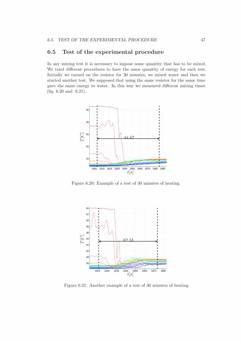
In any mixing test it is necessary to impose some quantity that has to be mixed.We tried different procedures to have the same quantity of energy for each test.Initially we turned on the resistor for 30 minutes, we mixed water and then westarted another test. We supposed that using the same resistor for the same timegave the same energy to water. In this way we measured different mixing times(fig. 6.20 and 6.21).

1800 1810 1820 1830 1840 1850 1860 1870 1880 1890

25

30

35

40

45

t[s]

T[C

]

81.67

Figure 6.20: Example of a test of 30 minutes of heating

1810 1820 1830 1840 1850 1860 1870 1880

26

28

30

32

34

36

38

40

42

44

t[s]

T[C

]

62.33

Figure 6.21: Another example of a test of 30 minutes of heating


The problem is that with a high initial average temperature the mixing timedecreases because the resistor gives less energy to the system. We can calculatethe energy given to the system in this way:

Q(t) =N∑

1

mi · c · (Ti(t)− T ii ) (6.3)

Q(t) = m · c ·N∑

1

27(Ti(t)− T i

i )

27(6.4)

Q(t) = m · c ·N

[

N∑

1

Ti(t)

N−

N∑

1

T ii

N

]

(6.5)

Q(t) = m · c ·N · (Ta(t)− T ia) = N · c ·m ·∆Ta(t) = c · ρ · V ·∆Ta(t) (6.6)

Imposing the same variation of the average temperature in each test you havethe same energy7 given to the system. We tried imposing a variation of 1.5°C andwe obtained optimal results using this method.

6.6 Calibration of the current sensor

We tested the current sensor with all the configurations to calibrate it. We mea-sured the current as a function of motor velocity.

0 2 4 6 8 10 120

0.2

0.4

0.6

0.8

1

1.2

1.4

rps[1/s]

Figure 6.22: Current on rps for free slinky+

7approximately 35800J

6.7. ESTIMATION ERRORS 49

In figure 6.22 the red line is the voltage output of the current sensor (is [V]),the blue one is the value of the power supply current (ip [A])8. We knew that thissensor has a sensitivity of 185 mV/A and so we calculated the green line that isthe value of measured current (im [A]).

We calculated similar curves for the other three configurations.

6.7 Estimation errors

We qualified the mixer measuring these characteristics: mixing time electric power consumption energy consumption

Mixing time We calculate the start of the mixing time using the motor datawhich were acquired at a rate of 1KHz which means a negligible error of 0.001 s.The end of the mixing was found studying the STD. Temperatures were acquiredat a rate of 3Hz. In the equation of STD we used the values of T f

i , Ti(t) and

T fa . It is supposed that the average temperature has not time error because of its

stability. T fi and Ti(t) has the same error time in fact T f

i = Ti(tend). We assumedthat the total error of mixing time was 2

3s.

Electric power consumption We calculated the electric power consumptionas the product of the voltage and current of the motor. The relative error of thecurrent is 1.5% 9. We assumed that the voltage error is 0.01V as the least step ofthe power supply.

∆W

W=

∆imim

+∆Vm

Vm+

∆im∆Vm

W(6.7)

Energy consumption We calculated energy consumption as the product of themixing time and the electric power consumption.

∆E

E=

∆W

W+

∆tmtm

+∆W∆tm

E(6.8)

The main part of the error came from the error of the tm. When it decreases itsrelative error increases.

8read directly on the power supply9from the data-sheet of the ACS712

Chapter 7

Experimental Data

7.1 Case 1: free slinky+

The first configuration we studied is the slinky+. We made several tests withthis configuration to validate the experimental setup. The movement of the slinkypresent different characteristics according to the rotational speed. At low rpm itlooked like an helical impeller because it had only rotational velocity. At highvelocity it reached its low end because of lift. In the mid range it had a verycomplex movement: it rotated and moved axially in the cylinder.

We tested the mixer with these value of Vm : (1,2,3,4,5,6,7,8)V . Finally weused these values (1.30,9.5,11)V to improve the graph of tm.

We decided to implement a simple system to acquire the rps real-time to controlthe motor before every test. When we finished all the tests we had the set of rpsto test the other configurations.

rps tm Wm E ∆W/W ∆E/E

0.53 316.67 0.2177 68.93 0.0055 0.03710.70 163.67 0.3314 54.24 0.0075 0.03911.09 55.44 0.4471 24.78 0.0093 0.06011.78 29.34 0.5794 16.99 0.0110 0.08162.05 28.84 0.7110 20.50 0.0132 0.07482.83 34.83 0.9421 32.81 0.0167 0.05773.66 23.25 1.2901 29.99 0.0221 0.06884.83 20.34 1.8764 38.15 0.0313 0.06775.64 14.67 2.2168 32.50 0.0364 0.08356.51 13.17 2.4588 31.96 0.0400 0.08977.95 14.50 3.3123 48.02 0.0532 0.07709.28 14.50 4.0689 58.99 0.0647 0.0743

Table 7.1: Mixing data of slinky+

51

52 CHAPTER 7. EXPERIMENTAL DATA

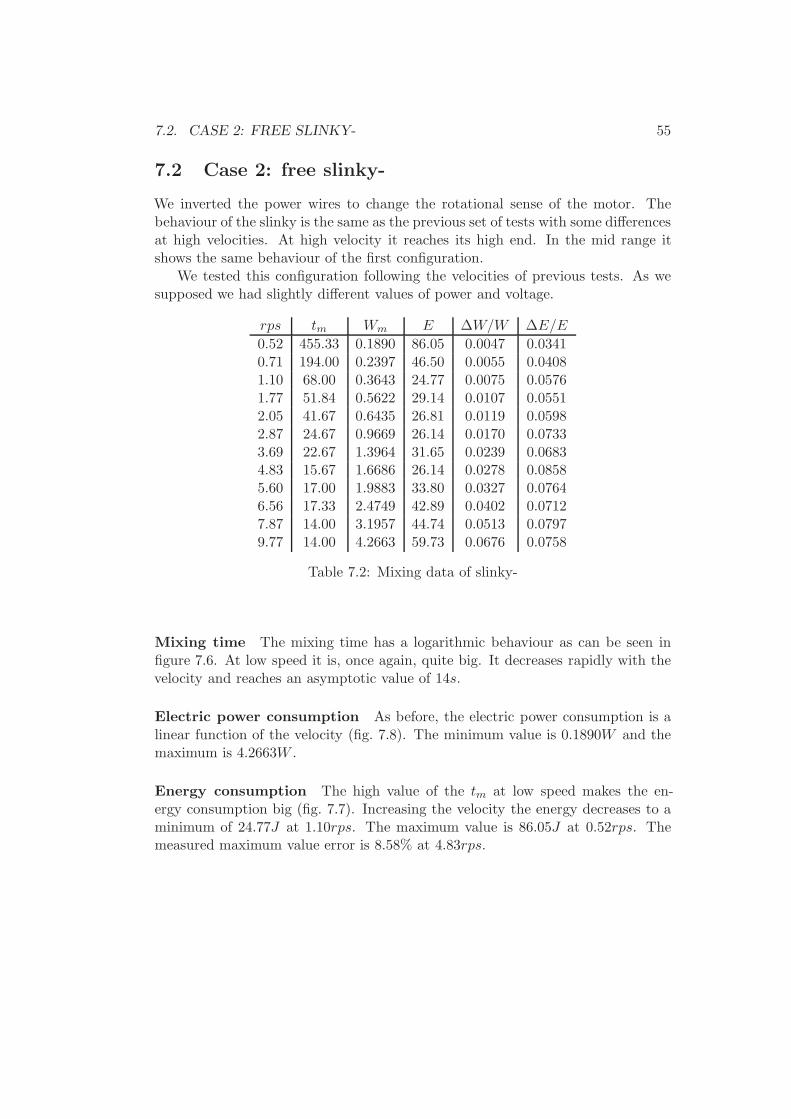
Mixing time As can be seen from figure 7.2 the mixing time has a logarithmicbehaviour. At low speed it is quite big and this means that mixer is not workingproperly. It decreases rapidly with the velocity and reaches an asymptotic valueof 14s.

0 2 4 6 8 100

50

100

150

200

250

300

350

rps[1/s]

t m[s]

Figure 7.1: tm of slinky+

Electric power consumption The electric power consumption grows linearlywith the velocity (fig. 7.4). The minimum value is 0.2177W and the maximum is4.0689W .

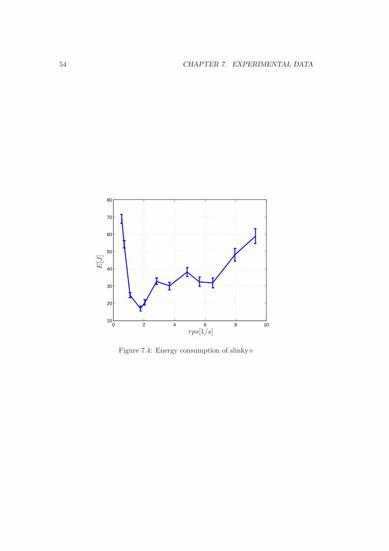
Energy consumption The high value of the tm at low speed makes the energyconsumption big. Increasing the velocity the energy decreases to a minimum of16.99J at 1.78rps. The maximum value is 68.93J at 0.53rps. The maximummeasured relative error is 8.97% at 6.51rps. It’s interesting because it has threeminima, two of which relative.

7.1. CASE 1: FREE SLINKY+ 53

100

101

102

103

rps[1/s]

t m[s]

Figure 7.2: Logarithmic graph of tm of slinky+

0 2 4 6 8 100

0.5

1

1.5

2

2.5

3

3.5

4

4.5

rps[1/s]

Wm[W

]

Figure 7.3: Electric power consumption of slinky+


0 2 4 6 8 1010

20

30

40

50

60

70

80

rps[1/s]

E[J]

Figure 7.4: Energy consumption of slinky+

7.2. CASE 2: FREE SLINKY- 55

7.2 Case 2: free slinky-

We inverted the power wires to change the rotational sense of the motor. Thebehaviour of the slinky is the same as the previous set of tests with some differencesat high velocities. At high velocity it reaches its high end. In the mid range itshows the same behaviour of the first configuration.

We tested this configuration following the velocities of previous tests. As wesupposed we had slightly different values of power and voltage.


0.52 455.33 0.1890 86.05 0.0047 0.03410.71 194.00 0.2397 46.50 0.0055 0.04081.10 68.00 0.3643 24.77 0.0075 0.05761.77 51.84 0.5622 29.14 0.0107 0.05512.05 41.67 0.6435 26.81 0.0119 0.05982.87 24.67 0.9669 26.14 0.0170 0.07333.69 22.67 1.3964 31.65 0.0239 0.06834.83 15.67 1.6686 26.14 0.0278 0.08585.60 17.00 1.9883 33.80 0.0327 0.07646.56 17.33 2.4749 42.89 0.0402 0.07127.87 14.00 3.1957 44.74 0.0513 0.07979.77 14.00 4.2663 59.73 0.0676 0.0758

Table 7.2: Mixing data of slinky-

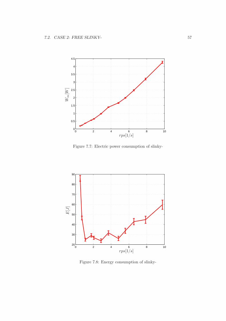
Mixing time The mixing time has a logarithmic behaviour as can be seen infigure 7.6. At low speed it is, once again, quite big. It decreases rapidly with thevelocity and reaches an asymptotic value of 14s.

Electric power consumption As before, the electric power consumption is alinear function of the velocity (fig. 7.8). The minimum value is 0.1890W and themaximum is 4.2663W .

Energy consumption The high value of the tm at low speed makes the en-ergy consumption big (fig. 7.7). Increasing the velocity the energy decreases to aminimum of 24.77J at 1.10rps. The maximum value is 86.05J at 0.52rps. Themeasured maximum value error is 8.58% at 4.83rps.


0 2 4 6 8 100

50

100

150

200

250

300

350

400

450

500

rps[1/s]

t m[s]

Figure 7.5: tm for slinky-

100

101

102

103

rps[1/s]

t m[s]

Figure 7.6: Logarithmic graph of tm of slinky-

7.2. CASE 2: FREE SLINKY- 57

0 2 4 6 8 100

0.5

1

1.5

2

2.5

3

3.5

4

4.5

rps[1/s]

Wm[W

]

Figure 7.7: Electric power consumption of slinky-

0 2 4 6 8 1020

30

40

50

60

70

80

90

rps[1/s]

E[J]

Figure 7.8: Energy consumption of slinky-

7.3. CASE 3: FIXED SLINKY 59

7.3 Case 3: fixed slinky

We decide to fix the slinky to avoid axial movements. This is a simple test toverify the influence of the described movements on the performance of the mixer.We used some plastic cable ties to fix the slinky to the shaft.

We tested the mixer at the following velocities.


0.50 345.00 0.2545 87.80 0.0062 0.03401.09 90.00 0.4580 41.22 0.0093 0.04412.05 36.00 0.7448 26.81 0.0137 0.06233.68 27.17 1.4490 37.19 0.0247 0.05914.77 25.17 2.0477 51.54 0.0340 0.05675.60 20.33 2.4034 48.86 0.0394 0.06366.54 18.33 2.9978 54.94 0.0486 0.06567.99 16.67 3.6686 61.15 0.0588 0.06799.43 11.33 5.1047 57.83 0.0810 0.0876

Table 7.3: Mixing data of fixed slinky

Mixing time In this configuration the mixing time decrease logarithmicly as inthe the other tests (fig. 7.10). At low speed, once again, the mixer is not workingproperly. It decreases rapidly as the velocity increase.

Electric power consumption As previous tests the electric power consumptiondepends linearly on the velocity (fig. 7.12). The minimum value is 0.2545W andthe maximum is 5.1047W .

Energy consumption At low speedthe energy consumption is big (fig. 7.11)because of the high value of tm. Increasing the velocity the energy decreases toa minimum of 26.81J at 2.05rps. The maximum value is 87.80J at 0.50rps. Themeasured relative error increased with velocity and its maximum value is 8.76%at 9.43rps.


0 2 4 6 8 100

50

100

150

200

250

300

350

rps[1/s]

t m[s]

Figure 7.9: tm for fixed slinky

100

101

102

103

rps[1/s]

t m[s]

Figure 7.10: Logarithmic graph of tm of fixed slinky

7.3. CASE 3: FIXED SLINKY 61

0 2 4 6 8 100

1

2

3

4

5

6

rps[1/s]

Wm[W

]

Figure 7.11: Electric power consumption of fixed slinky

0 2 4 6 8 1020

30

40

50

60

70

80

90

100

rps[1/s]

E[J]

Figure 7.12: Energy consumption of fixed slinky

7.4. CASE 4: IMPELLER 63

7.4 Case 4: impeller

After the tests with the slinky we mounted an impeller on the shaft. We decidedto make the initial tests with an impeller taken from an old pc fan. It was idealto create the axial flow field needed because of the height ratio H/D of the mixer.

We tested the mixer following the velocities of previous tests with some limita-tions at high velocities.

rps tm Wm E ∆W/W ∆E/E Re[104]

0.45 48.33 0.3020 14.59 0.0071 0.0835 0.64801.03 22.33 0.5268 11.59 0.0106 0.1076 1.48322.14 16.33 0.8024 13.10 0.0146 0.1110 3.08162.95 16.00 1.6084 25.73 0.0280 0.0861 4.24804.00 10.33 3.7958 39.21 0.0634 0.0999 5.76005.68 10.67 6.6813 71.22 0.1081 0.0895 8.17926.56 12.66 10.4435 132.21 0.1670 0.0750 9.1164

Table 7.4: Mixing data of impeller

Mixing time Also in this case the mixing time has a logarithmic behaviour ascan be seen in figure 7.14. At low speed it is significantly smaller than in theothers configurations. It decreases with the velocity.

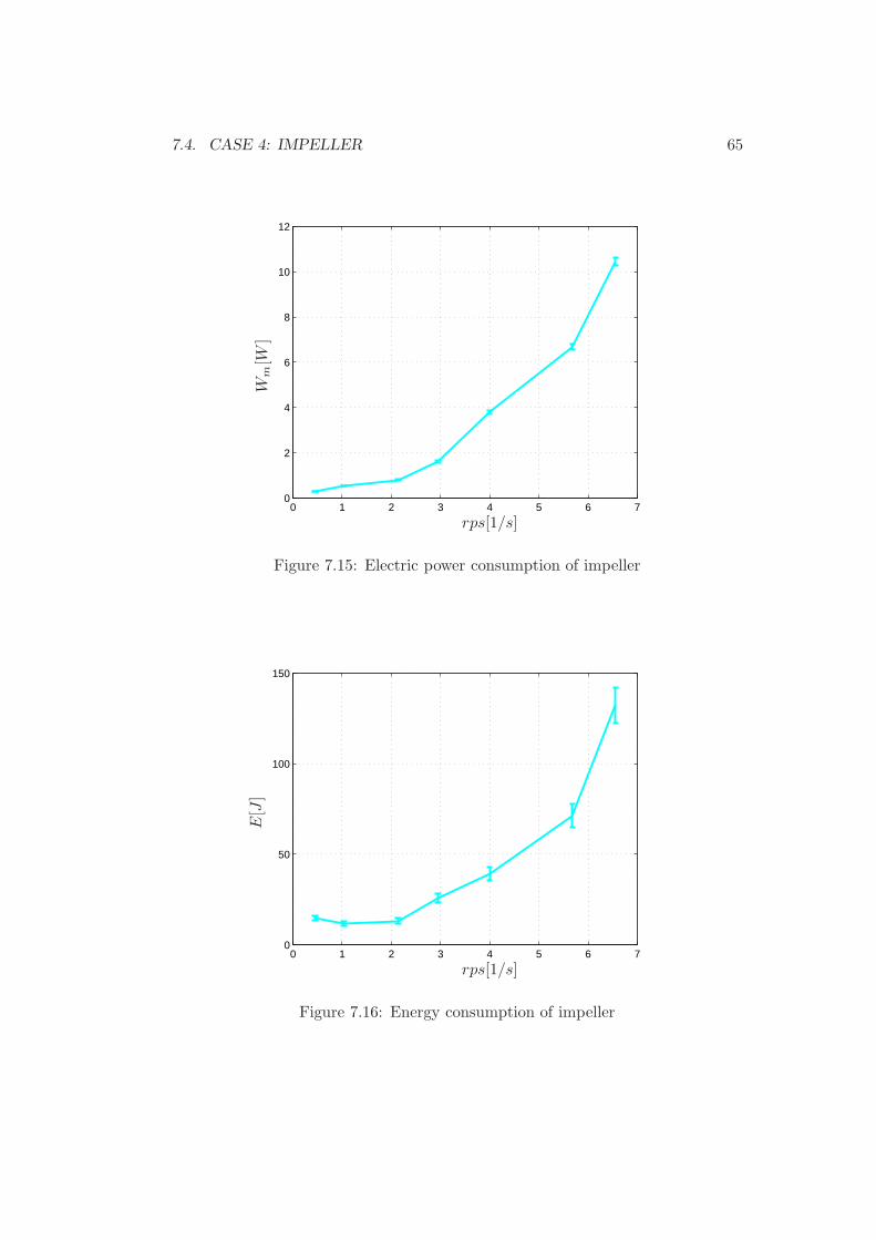
Electric power consumption The electric power consumption is an exponen-tial function of the velocity (fig. 7.15). Its minimum value is 0.3020W and themaximum is 10.4435W .

Energy consumption The high value of the Wm at high velocities results inan higher power consumption (fig. 7.16). The energy has a minimum of 11.59Jat 1.03rps. The maximum value is 132.21J at 6.56rps. In the condition of bestefficiency it has a relative error of 10.76%.


0 1 2 3 4 5 6 710

15

20

25

30

35

40

45

50

rps[1/s]

t m[s]

Figure 7.13: tm for impeller

100

101.1

101.2

101.3

101.4

101.5

101.6

rps[1/s]

t m[s]

Figure 7.14: Logarithmic graph of tm for impeller

7.4. CASE 4: IMPELLER 65

0 1 2 3 4 5 6 70

2

4

6

8

10

12

rps[1/s]

Wm[W

]

Figure 7.15: Electric power consumption of impeller

0 1 2 3 4 5 6 70

50

100

150

rps[1/s]

E[J]

Figure 7.16: Energy consumption of impeller

7.5. COMPARISON 67

7.5 Comparison

The aim of this work was to qualify this kind of new mixer. The comparison ofthe different configurations shows some interesting elements.

Mixing time The tm of the impeller is always smaller than the tm of otherconfigurations at every velocity (fig. 7.17).

Electric power consumption At low velocities there are not differences be-tween various configurations. After 3rps the Wm of the impeller increases expo-nentially and becomes three times higher than the value of the slinky configurationsWm (fig. 7.19). We stopped before 7rps because the power request exceeded the ca-pabilities of our powe supply. This increase was probably caused by hydrodynamicresistance.

0 2 4 6 8 100

50

100

150

200

250

300

350

400

450

500

rps[1/s]

t m[s]

Figure 7.17: Comparison of tm

Energy consumption This graph is probably the most useful piece of infor-mation of this work (fig. 7.20). You can see that the fixed slinky is worse thanboth the free slinky configurations. So we can say that the axial movements of thespring reduce the energy consumption. The slinky reaches higher velocities thanthe impeller thanks to its smaller power consumption.


100

101

102

103

rps[1/s]

t m[s]

Figure 7.18: Logarithmic graph of comparison of tm

0 2 4 6 8 100

2

4

6

8

10

12

rps[1/s]

Wm[W

]

Figure 7.19: Comparison of electric power consumption

7.5. COMPARISON 69

0 2 4 6 8 100

50

100

150

rps[1/s]

E[J]

Figure 7.20: Comparison of energy consumption

Chapter 8

Conclusions

8.1 Achievements

The present work was entirely developed in the thermofluid dynamics laboratoryof the University of Studies of Brescia. The aim of this dissertation was thestudy of an unconventional turbulent mixer and compare it with a classic impellerconfiguration. We tested the mixer performance using measures of temperatureand mix water at different temperatures.

The first point of the work was the design and the construction of the mixer.We tried to create a versatile structure that could be improved during the work.The mixer that we created is composed by few parts that can be easily replaced ifnecessary. In this way mixer could be used in different tests.

The second step was to add temperatures sensors and a heat exchanger system.We placed twenty-seven thermocouples along the height of the mixer. Knowingthe temperatures of every layer of the mixer allowed us to have useful informationsto do more complete tests. Preliminarily we used a thermostatic bath to cool thebottom of the water to test the sensors’ system. In main tests we used a resistoras heating system to heat the top layer of the cylinder. Using a heating systeminstead of a cooling system allowed us to make faster tests.

Finally we developed an experimental procedure to make the measures we werelooking for: mixing time and electric power consumption. We used the velocityas reference for each test. We tested four different configurations. None of theconfigurations has been optimized because of the great number of tests necessaryto qualify the systems.

The results of the experiments are satisfactory. In every configuration trendof the mixing time as a function of the rotation speed is a logarithmic type inagreement with the literature (fig. 7.18). The configuration equipped with impellerpresents mixing times lower but an electric power consumption higher than theone with spring. In terms of energy consumption , the propeller system is efficientat low speeds, the spring is efficient at high speeds (fig. 7.20).

Results of this work permitted us to make some important considerations. Allthe measures of the mixing time were made as function of velocity, so you can

71

72 CHAPTER 8. CONCLUSIONS

use another motor to make the same measures. The measures of electric powerconsumption were done in succession after all the tests. These results don’t saythe real power consumption for mixing but the consumption of the motor we usedin our tests. They can be used to compare different configurations.

8.2 Future developments

This work demonstrated the feasibility of a mixer equipped with slinky spring formixing liquids and justifies possible future searches for a better understanding ofthe dynamics of the mixing taking place in it.

All the data acquired in these tests could be analysed to find some other infor-mations. For example you can study which thermocouples are relevant to describethe mixing making a statistical work or you can calculate the mixing time withsmaller or greater degree of homogeneity.

It would be interesting to make some visualization tests, like Mavros in [10],tounderstand the variation of the flow field caused by the slinky movement. Thisknowledge could enable us to use a little number of sensors.

You can qualify a mixer by measuring degree of mechanical damage. This is avery important factor in a lot of mixing processes (as shown by Papoutsakis in[7]).It is supposed that little electric power consumption of the slinky is caused by asmaller mechanical damage than the system with the impeller.

The final step could be development of a campaign of tests to optimize themixer.


Notations

c specific heat

D diameter of the impeller

Dc diameter of the mixer cylinder

E energy consumption

H heigth of the cylinder

mi mass of i-th layer

N number of thermocouples

Ni number of i-th thermocouple

Nt dimensionless mixing time

im measured current

ip power supply current

is output of the current sensor

Q heat

Re Reynolds number

rps round per seconds

slinky+ free slinky that moves counter-clockwise

slinky− free slinky that moves clockwise

STD standard deviation

tend final time of a test

tm mixing time

T ia initial average temperature

T fa final average temperature

T ii initial temperature of i-th thermocouple

T fi final temperature of i-th thermocouple

8.2. FUTURE DEVELOPMENTS 75

T ′ derivative on time of temperature

V volume of the cylinder

Vcc supply voltage

Vm motor voltage

Wm electric power consumption

α thermal diffusivity

∆im measured current error

∆Vm motor voltage error

∆W electric power consumption error

∆T fi difference between T f

i and T fa

∆T toti difference between T i

a and T fa

λ thermal conductivity

µ dynamic viscosity

ρ density

Bibliography

[1] F. Ippolito F. Scargliati A. Brucato A.Busciglio, F. Grisafi. Mixing time inunbaffled stirred tanks. In 14th European Conference on Mixing, 2012.

[2] Dassault Systemes SolidWorks Corporation, 300 Baker Avenue, Concord, MA01742 USA. Guida dello studente per l’apprendimento del software Solid-Works.

[3] Suzanne M.Kresta Edward L.Paul, Victor A.Atimeo-Obeng. Handbook ofindustrial mixing : science and practice. Wiley Interscience, 2004.

[4] Ivan Fort and Tomas Jirout. A study on blending characteristics of axial flowimpellers. Chemical and Process Engineering, 32:311–319, 2011.

[5] Hans-Petter Halvorsen. Data acquisition in labview, 2011.

[6] John H. Lienhard IV John H. Lienhard IV. A heat transfer textbook. Phlogis-ton Press, third edition, 2008.

[7] Eleftherios T. Papoutsakis. Fluid-mechanical damage of animal cells in biore-actor. Tibtech, 9:427–437, 1991.

[8] Aniruddha B. Pandit Parag R. Gogate, Anthony A.C.M. Beenackers.Multiple-impeller systems with a special emphasis on bioreactors: a criticalreview. Biochemical Engineering Journal, pages 109–144, 2000.

[9] Francesco Pasqua. Analisi sperimentale preliminare di un dispositivo innova-tivo per il mixing turbolento, 2011.

[10] P.Mavros. Flow visualization in stirred vessels - a review of experimentaltechniques. Trans ICHemE, 79:113–127, 2001.

[11] I. Fort T. Jirout F. Riege R. Allner R. Sperling. Study of the blending efficencyof pitched blade impellers. Acta Polytechnica, 41(6):7–13, 2001.

77

78 BIBLIOGRAPHY

Ringraziamenti

Innanzitutto ringrazio i professori Maurizio Quadrio e Pietro Poesio per l’ op-portunita che mi hanno concesso nel realizzare questo lavoro di tesi. Entrambisono sempre stati disponibili ad aiutarmi nel mio cammino.

Merito di questa ricerca va anche, e direi soprattutto, al dottorando StefanoFarise che mi ha assistito fin dall’inizio di questa mia avventura all’universita diBrescia. Non c’e stato giorno in cui non mi abbia insegnato qualcosa di nuovo emi sento molto fortunato di aver condiviso il suo ultimo anno da dottorando.

Ringrazio tutti i ragazzi dei laboratori di Brescia, in particolar modo l’ing.Marco De Mori per le continue assistenze in ambito elettronico.

Ringrazio la mia famiglia per il continuo supporto che mi ha dato in questianni. I miei genitori che sono sempre stati un esempio per me. Mia sorella che,in ogni occasione, e stata pronta ad aiutarmi, sin dall’inizio della mia carrierauniversitaria. Mio fratello che non ha mai smesso di credere nelle mie capacita.I miei nipoti che riescono sempre a tirarmi su di morale. I miei zii per avermiincoraggiato. Zio Elio che mi ha insegnato cosa significhi essere un bravo zio. ZiaLia sempre pronta a chiamarmi per sapere come andavano le cose. Zia Gina chenonostante la lontananza riesce sempre a farsi sentire vicina. Tutti i miei cugini,in particolar modo Fabiana.

Vorrei ringraziare tutti i miei compagni di universita. Finito questo percorsopotro chiamarli per quello che sono diventati, degli amici insostituibili. Primo fratutti Alain che dopo tutto questo tempo ormai e diventato come un secondo fratello.Francesco con cui ho condiviso la mia passione per il mondo automobilistico. Marcoche mi ha sopportato a lungo durante i viaggi in treno. Matteo sempre pronto aconfrontarsi durante le sessioni di studio. Il gruppo dei Dronisti con cui ho passatoun piacevole anno. Infine tutti gli altri compagni di universita.

Ringrazio tutti i miei amici che non vedevano l’ora che arrivasse questo mo-mento. I miei migliori amici, Alice e Giovanni. La prima per le continue uscitea chiacchierare, il secondo perche non esistono persone come lui. Andrea per leserate passate a filosofeggiare. Fabio sempre pronto ad offrirmi un caffe e fare duechiacchiere. Dan con cui ho condiviso molte sessioni di studio. Stefano, Giuseppe,Dorina e tutti gli altri amici.

Infine ringrazio tutte le persone che ho avuto modo di conoscere in questi annidi universita e che mi hanno aiutato a crescere.

POLITECNICO DI MILANO · Introduzione 1.1 L’importanza del mixing Attualmente il mixing come...

Documents

Transcript of POLITECNICO DI MILANO · Introduzione 1.1 L’importanza del mixing Attualmente il mixing come...