Polarized Neutrons Intro and Techniques · History of Polarized Neutrons 1937"Theory of neutron...
38
Polarized Neutrons Intro and Techniques Ross Stewart
Transcript of Polarized Neutrons Intro and Techniques · History of Polarized Neutrons 1937"Theory of neutron...

Polarized NeutronsIntro and Techniques
Ross Stewart

| "i
| #i
Polarized neutron beamsEach individual neutron has spin s=½ and an angular momentum of ±½ħEach neutron has a spin vector and we define the polarization of a neutron beam as the ensemble average over all the neutron spin vectors, normalised to their modulus
+½ħ
-½ħ
“Spin-up”
“Spin-down”
B
If we apply an external field (quantisation axis) then there are only two possible orientations of the neutrons: parallel and anti-parallel to the field. The polarization can then be expressed as a scalar:
where there are N+ neutrons with spin-up and N- neutrons
with spin-down

History of Polarized Neutrons
1937 Theory of neutron polarization by a ferromagnet Schwinger (Phys Rev, 51, 544)
1938 Partial polarization of a neutron beam by passage through iron Frisch et al (Phys Rev 53, 719), Powers (Phys Rev 54, 827)
1937 - 1941 Theory of magnetic neutron scattering Halpern and Johnson (Phys Rev 51, 992; 52, 52; 55, 898)
1940 Magnetic moment of the neutron determined by polarization analysis Alvarez and Bloch (Phys Rev 57,111)
1932 Discovery of the neutron Chadwick (Proc Roy Soc A136 692)
1951 Polarizing mirrors, proof of the neutron’s μ.B interaction Hughes and Burgy (Phys Rev, 81, 498)

History of Polarized Neutrons1951 Polarizing crystals (magnetite Fe3O4, Co92Fe8)
Shull et al (Phys Rev 83, 333; 84, 912)
1959 First polarized beam measurements (of magnetic form factors of Ni and Fe) Nathans et al (Phys Rev Lett, 2, 254)
1963 General theory of neutron polarization analysis Blume (Phys Rev 130, 1670) Maleyev (Sov. Phys.: Solid State 4, 2533)
1969 First implementation of neutron polarization analysis, Oak Ridge, USA Moon, Riste and Koehler (Phys Rev 181, 920)
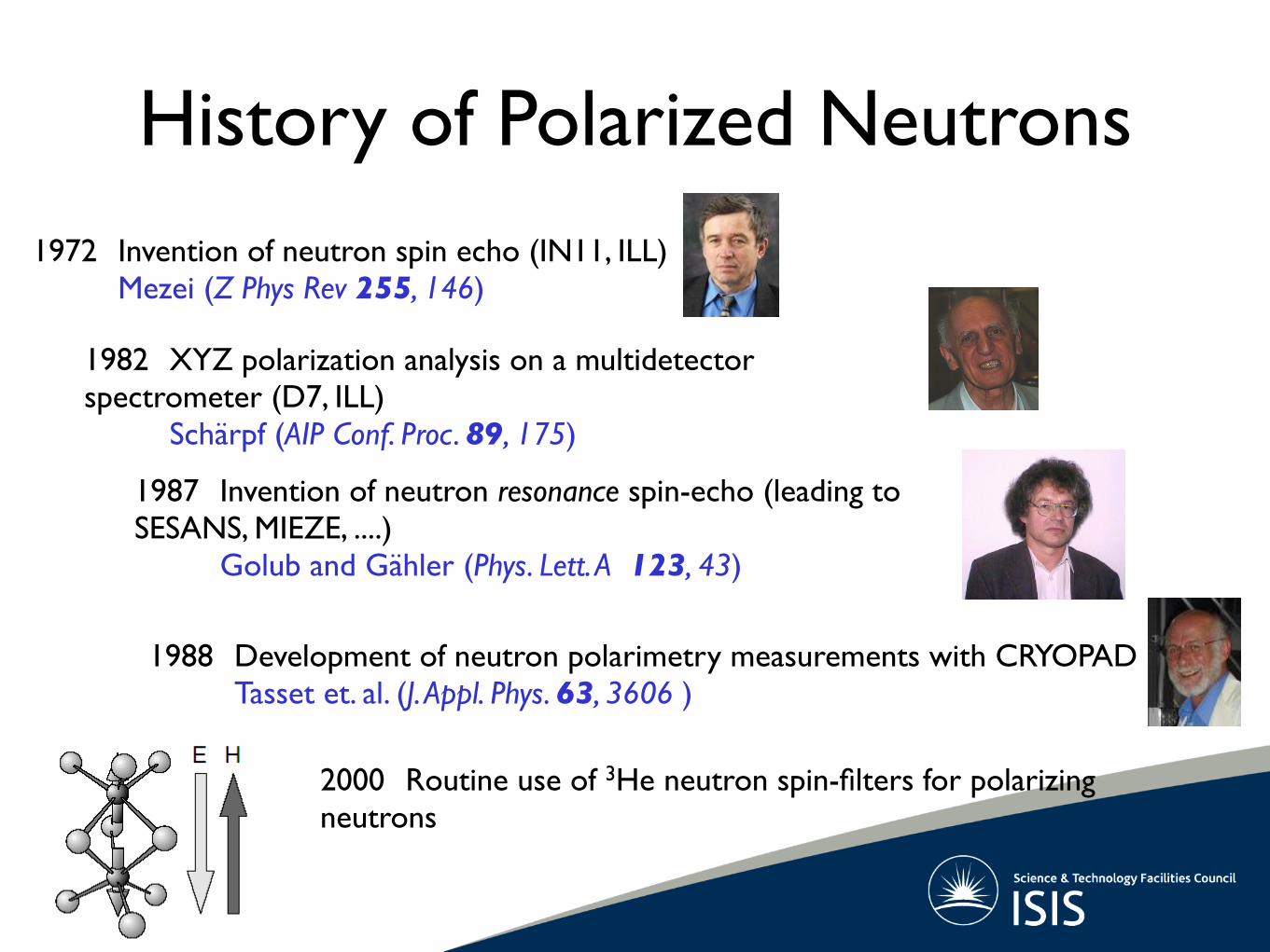
History of Polarized Neutrons1972 Invention of neutron spin echo (IN11, ILL) Mezei (Z Phys Rev 255, 146)
1982 XYZ polarization analysis on a multidetector spectrometer (D7, ILL) Schärpf (AIP Conf. Proc. 89, 175)
1988 Development of neutron polarimetry measurements with CRYOPAD Tasset et. al. (J. Appl. Phys. 63, 3606 )
2000 Routine use of 3He neutron spin-filters for polarizing neutrons
1987 Invention of neutron resonance spin-echo (leading to SESANS, MIEZE, ....) Golub and Gähler (Phys. Lett. A 123, 43)

Polarized neutrons today
• Single crystal diffraction• Diffuse scattering• Inelastic scattering (3-axis and TOF)• Reflectometry (on and off-specular)• SANS - magnetic and non-magnetic• Neutron Spin-Echo• Neutron Resonance Spin-Echo• SESANS• Larmor Diffraction• Neutron Depolarization• Polarized Neutron Tomography• ......

Polarized neutron beams
This description of a polarized beam is OK for experiments in which a single quantisation axis is defined: Longitudinal Polarization Analysis
The technique of 3-dimensional neutron polarimetry, however is termed:Vector (or Spherical) Polarization Analysis
€
P =N+ − N−
N+ − N−
=N+ /N−( ) −1N+ /N−( ) +1
=F −1F +1
Where is called the Flipping Ratio and is a measurable quantity in a
scattering experiment
€
F =N+
N−
What we often would like to do in polarized neutron experiments is measure the scalar polarization of the beam.

A Uniaxial PA experiment
analyserpolarizer
flipper 1
flipper 2
detector
B
|"i ! |"i
•First attempted by Moon, Riste and Koehler (Oak Ridge 1969)Phys Rev. 181 (1969) 920

A Uniaxial PA experiment
analyserpolarizer
flipper 1
flipper 2
detector
B
|"i ! |"i |#i ! |"i
•First attempted by Moon, Riste and Koehler (Oak Ridge 1969)Phys Rev. 181 (1969) 920

A Uniaxial PA experiment
analyserpolarizer
flipper 1
flipper 2
detector
B
|"i ! |"i |#i ! |"i|"i ! |#i
•First attempted by Moon, Riste and Koehler (Oak Ridge 1969)Phys Rev. 181 (1969) 920

A Uniaxial PA experiment
analyserpolarizer
flipper 1
flipper 2
detector
B
|"i ! |"i |#i ! |"i|"i ! |#i|#i ! |#i
•First attempted by Moon, Riste and Koehler (Oak Ridge 1969)Phys Rev. 181 (1969) 920

A Uniaxial PA experiment
analyserpolarizer
flipper 1
flipper 2
detector
B
|"i ! |"i |#i ! |"i|"i ! |#i|#i ! |#i}
“Non-spin-flip”}
“Spin-flip”•First attempted by Moon, Riste and Koehler (Oak Ridge 1969)
Phys Rev. 181 (1969) 920

PolarizersStern-Gerlach experiment (1922)
3He spin-filter
Cu2MnAl (Heusler) crystal grown at ILL
Supermirror systems(eg Co/Ti, Fe/Si etc)
d1}
λ 1λ 2λ 3λ 4
λ c
d2} d3}
d4}

IBF
BG BG
- BG
BF
BC
y
z BG BG
BF
d
FlippersDrabkin flipper: useful for white beams of limited size
Bout
PoutPin
Bin
Dabbs Foil: “current sheet”
Mezei Flipper: “current sheet”
AFP Flipper: “adiabatic fast passage”

Uniaxial Polarization Analysis

Neutron polarization and scattering
We start with the (elastic - |ki| = |kf|) scattering cross-section
Where the spin-state of the neutron S is either spin-up or spin down
€
dσdΩ
=mn
2π2⎛
⎝ ⎜
⎞
⎠ ⎟ ʹ′ k ʹ′ S V kS 2
€
↑ =10⎛
⎝ ⎜ ⎞
⎠ ⎟
€
↓ =01⎛
⎝ ⎜ ⎞
⎠ ⎟
For nuclear scattering (no spin) V is the Fermi pseudopotential, and the matrix element is
where we have used the fact that the spin states are orthogonal and normalised
€
ʹ′ S b S = b ʹ′ S S =
b ↑ → ↑
↓ → ↓
⎧ ⎨ ⎩
⎫ ⎬ ⎭
0 ↑ → ↓
↓ → ↑
⎧ ⎨ ⎩
⎫ ⎬ ⎭
⎧
⎨
⎪ ⎪
⎩
⎪ ⎪
Non-spin-flip
Spin-flip
€
↑↓ = ↓↑ = 0, ↑↑ = ↓↓ =1

Neutron polarization and magnetic scattering
(see e.g. Squires)
V is the magnetic scattering potential given by
where ζ = x, y, z. Here M⊥(Q) represents the component of the Fourier transform of the magnetisation of the sample, which is perpendicular to the scattering vector Q - i.e. the neutron sensitive part. σζ are the Pauli spin matrices€
Vm (Q) = −γ nr02µB
σ ⋅M⊥ (Q) = −γ nr02µB
σζ ⋅ M⊥ζ (Q)ζ
∑
€
σx =0 11 0⎛
⎝ ⎜
⎞
⎠ ⎟ , σy =
0 − ii 0⎛
⎝ ⎜
⎞
⎠ ⎟ , σ z =
1 00 −1⎛
⎝ ⎜
⎞
⎠ ⎟
Substitution of these into the magnetic potential gives us the matrix elements
€
ʹ′ S Vm (Q) S = −γ nr02µB
M⊥z (Q)−M⊥z (Q)
M⊥x (Q) − iM⊥y (Q)M⊥x (Q) + iM⊥y (Q)
↑ → ↑
↓ → ↓
⎫ ⎬ ⎭
↑ → ↓
↓ → ↑
⎫ ⎬ ⎭
⎧
⎨
⎪ ⎪
⎩
⎪ ⎪
Non-spin-flip
Spin-flip

Magnetic scattering rule
The non-spin-flip scattering is sensitive only to those components of the
magnetisation parallel to the neutron spin
The spin-flip scattering is sensitive only to those components of the magnetisation
perpendicular to the neutron spin
NB This is one of those points that you should take away with you. It is the basis of all magnetic polarization analysis techniques

Neutron polarization and nuclear scattering
In general a bound state is formed between the nucleus and the neutron during scattering with either spins antiparallel (spin-singlet) or spins parallel (spin-triplet). The scattering lengths for these situations are different and are termed b- and b+.
(see e.g. Squires, p173)
The scattering length operator is
€
ˆ b = A + Bσ ⋅ I
€
A =(I +1)b+ + Ib−
2I +1, B =
b+ − b−2I +1
The calculation of the matrix elements now proceeds analogously to the case of magnetic scattering
€
ʹ′ S ˆ b S =
A + BIzA − BIzB(Ix − iIy )B(Ix + iIy )
↑ → ↑
↓ → ↓
⎫ ⎬ ⎭
↑ → ↓
↓ → ↑
⎫ ⎬ ⎭
⎧
⎨
⎪ ⎪
⎩
⎪ ⎪
Non-spin-flip
Spin-flip
Since the nuclear spins are (normally) randomTherefore with the coherent scattering amplitude proportional to , we can write
€
b
€
Ix = Iy = Iz = 0
€
b = A i.e. the coherent scattering is entirely non-spin-flip

~M?( ~Q) = Q⇥⇣
~M( ~Q)⇥ Q⌘
= ~M( ~Q)�⇣
~M( ~Q) · Q⌘
Q
Moon-Riste-Koehler Equations
If the polarization is parallel to the scattering vector, then the magnetisation in the direction of the polarization will not be observed since the magnetic interaction vector is zero. i.e. all magnetic scattering will be spin-flip
Bringing all this together, we get
Moon, Riste and Koehler (Phys Rev 181 (1969) 920)
Remember that:
€
↑ → ↑ = b − γ nr02µB
M⊥z + BIz
↓ → ↓ = b + γ nr02µB
M⊥z − BIz
↑ → ↓ = −γ nr02µB
M⊥x − iM⊥y( ) + B Ix − iIy( )
↓ → ↑ = −γ nr02µB
M⊥x + iM⊥y( ) + B Ix + iIy( )

Spin-incoherent scattering
Isotope incoherent scattering spin incoherent scattering
The other transitions are dealt with in a similar way
Now, let’s take another look at the nuclear incoherent scattering. We know that this is given by
€
b2 − b ( )2
Applying this to the transition, and neglecting magnetic scattering, we get
€
↑ → ↑
€
b2 = b + BIz( )2
= b ( )2
+ B2Iz2 + 2 b BIz
Now, for a randomly oriented distribution of nuclei of spin I, we have
since the distribution is isotropic
€
I = I(I +1) = Ix2 + Iy
2 + Iz2
⇒ Ix2 = Iy
2 = Iz2 =
13I(I +1)
Therefore we can write
€
b2 − b ( )2
= b ( )2− b ( )
2+13
B2I(I +1)

Moon-Riste-Koehler IIFinally, we get
The details of the magnetic scattering will in general depend on the direction of the neutron polarization with respect to the scattering vector, and also on the nature of the orientation of the magnetic moments
where
€
↑ → ↑ = b − γ nr02µB
M⊥z + bII +13
bSI
↓ → ↓ = b + γ nr02µB
M⊥z + bII +13
bSI
↑ → ↓ = −γ nr02µB
M⊥x − iM⊥y( ) +23
bSI
↓ → ↑ = −γ nr02µB
M⊥x + iM⊥y( ) +23
bSI
€
bII = b ( )2− b ( )
2
bSI = B2I(I +1)

Scientific Examples

~M?( ~Q) = ~M( ~Q)�⇣
~M( ~Q) · Q⌘
Q = ~M( ~Q)
Polarized magnetic diffractionFor a ferromagnetic sample aligned in a field perpendicular to the scattering vector we have
and M⊥ has no component in the xy-plane, so that the spin-flip scattering is zero.This implies that we don’t need to analyse the neutron spin, it will always end upin the same direction it started in. Therefore
for neutrons polarized antiparallel to the field
for neutrons polarized parallel to the field
where€
dσ dΩ = FN (Q) − FM (Q)[ ]2
€
dσ dΩ = FN (Q) + FM (Q)[ ]2
€
FN (Q) = bi exp(iQ ⋅ ri)i∑
FM (Q) = γ nr0 gJi Ji f i(Q)exp(iQ ⋅ ri)i∑
Notice that to simulate an unpolarized measurement, we simply average the two polarized cross sections
NB we have neglected incoherent scattering here
€
dσdΩ
=12
FN (Q) − FM (Q)( )2+ FN (Q) + FM (Q)( )2[ ]
= FN2(Q) + FM
2 (Q)

After all the reflections have been measured, FM(Q) can be deduced (assuming careful measurements of FN(Q) have been taken - at low fields/high temps). Then FM(Q) can be inverse Fourier transformed to get the real-space magnetisation density
Ni
Polarized magnetic diffraction
So, for example, in the case of Ni we measure a flipping ratio of 1.7 at the (111) reflection and 1.1 at the (400) reflection
Using a spin flipper to access these two polarized cross sections we can determine the “flipping ratio”, R, of a particular Bragg reflection:
€
R =dσ dΩ( )⇓dσ dΩ( )⇑
=FN (Q) + FM (Q)[ ]2
FN (Q) − FM (Q)[ ]2=1+ γ1− γ⎛
⎝ ⎜
⎞
⎠ ⎟
2
€
γ =FM (Q)FN (Q)
with
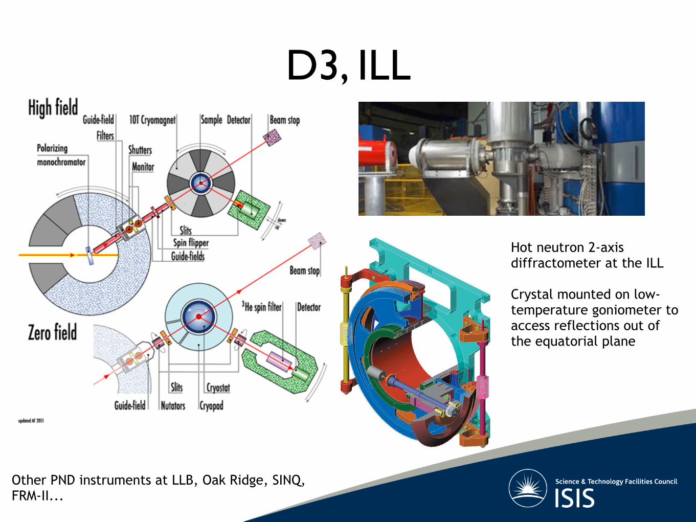
D3, ILL
Hot neutron 2-axis diffractometer at the ILL
Crystal mounted on low-temperature goniometer to access reflections out of the equatorial plane
Other PND instruments at LLB, Oak Ridge, SINQ,FRM-II...
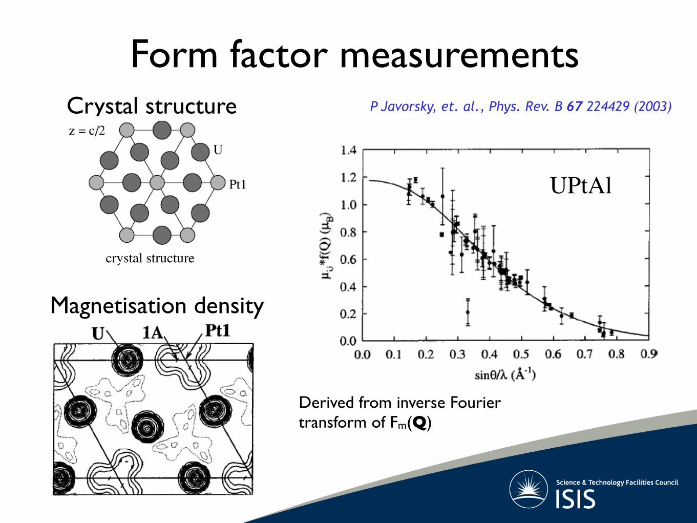
magnetic moment density!
UPtAl!P. Javorsky et al., Phys. Rev. B 67 (2003) 224429!
Crystal structure
crystal structure!Derived from Bragg peak positions/intensities
Magnetisation density
Derived from inverse Fourier transform of Fm(Q)
Form factor measurementsP Javorsky, et. al., Phys. Rev. B 67 224429 (2003)

Spin density measurements
4
FIG. 4: (Color online) a). Comparison of the form factorscalculated with the experimental atomic positions (zAs =0.3612) and theoretical energy optimized one (zAs = 0.3499).The arrow points to scattering vectors that provide evidencefor fairly strong anisotropy in the form factor. b). Experimen-tal form factors for SrFe2As2 and BCC Fe, and the calculatedform factors with the experimental As position.
form factors are quite similar, with di�erences showing up
at larger and more di⇤cult to measure scattering vectors.The similarity with bcc Fe is particularly evident in thetotal 3d charge density within the mu⇤n-tin sphere. Thisis 5.95 electrons for the experimental atomic positions inSrFe2As2, 6.02 electrons for the corresponding calculatedenergy optimized As position and 5.83 electrons for bccFe calculated with the same mu⇤n-tin radius.
We have determined the magnetic form factor of Fein SrFe2As2 by neutron di�raction experiments and de-duced the Fe magnetic moment as 1.04(1)µB. We alsocalculated the magnetic form factor by first principleselectronic structure methods using both the experimen-tal and optimized As positions. While the magnitudeof the calculated magnetic moments strongly depends onthe As position, the normalized magnetic form factorswere remarkably similar with each other and also agreedwell with the normalized magnetic form factors from theexperiment. The largest di�erence between the two the-oretical calculations was the noticeable increase in thespin anisotropy for the optimized As position. The ex-periments were limited by spectrometer geometry anddid not measure far enough in reciprocal space to accessthese contributions.
Research supported by the U.S. Department of Energy,O⇤ce of Basic Energy Sciences, Division of Materials Sci-ences and Engineering under Contract No. DE-AC02-07CH11358.
1 T. C. Leung, X. W. Wang, and B. N. Harmon, Phys. Rev.B 37, 384 (1988).
2 W. E. Pickett, Rev. Mod. Phys. 61, 433 (1989).3 A Kreyssig, M. A. Green, Y. Lee, G. D. Samolyuk, P.Zajdel, J. W. Lynn, S. L. Bud’ko, M. S. Torikachvili, N.Ni, S. Nandi, J. B. Leao, S. J. Poulton, D. N. Argyriou,B. N. Harmon, R. J. McQueeney, P.C. Canfield, and A. I.Goldman, Phys. Rev. B 78, 184517 (2008).
4 A. I. Goldman, A. Kreyssig, K. Prokes, D. K. Pratt, D.N. Argyriou, J. W. Lynn, S. Nandi, S. A. J. Kimber, Y.Chen, Y. B. Lee, G. Samolyuk, J. B. Leao, S. J. Poulton,S. L. Bud’ko, N. Ni, P. C. Canfield, B. N. Harmon, and R.J. McQueeney, Phys. Rev. B 79, 024513 (2009).
5 I. I. Mazin, M. D. Johannes, L. Boeri, K. Koepernik, andD. J. Singh, Phys. Rev. B 78, 085104 (2008).
6 K. Kaneko, A. Hoser, N. Caroca-Canales, A. Jesche, C.Krellner, O. Stockert, and C. Geibel, Phys. Rev. B 78,212502 (2008).
7 J. Zhao, W. Ratcli�, J. W. Lynn, G. F. Chen, J. L. Luo, N.L. Wang, J. Hu, and P. Dai, Phys. Rev. B 78, 140504(R)(2008).
8 A. Jesche, N. Caroca-Canales, H. Rosner, H. Borrmann,A. Ormeci, D. Kasinathan, H. H. Klauss, H. Luetkens, R.Khasanov, A. Amato, A. Hoser, K. Kaneko, C. Krellner,and C. Geibel, Phys. Rev. B 78, 180504(R) (2008).
9 Marcus Tegel, Marianne Rotter, Veronika Weib, Falko MSchappacher, Rainter Pottgen and Dirk Johrendt, J. Phys.:Condens. Matter 20, 452201 (2008).
10 N. Ni, M. E. Tillman, J.-Q. Yan, A. Kracher, S. T. Han-nahs, S. L. Bud�ko, and P. C. Canfield, Phys. Rev. B 78,214515 (2008).
11 H.-F. Li, W. Tian, J. L. Zarestky, A. Kreyssig, N. Ni, S. L.Bud�ko, P. C. Canfield, A. I. Goldman, R. J. McQueeney,and D. Vaknin, Phys. Rev. B 80, 054407 (2009).
12 David J. Singh, Lars Nordstrom, Plane Waves, Pseudopo-tentials and LAPW method, Springer Science (2006).
13 P. Blaha, K. Schwarz, G. K. H. Madsen, D. Kvasnickaand J. Luitz, Wien2k, An augmented Plane Wave +Local Orbitals Program for Calculating Crystal Proper-ties (Karlheinz Schwarz, Techn. Universitat Wien, Aus-tria), 2001. For the spin density contours and the struc-ture figure, we used a graphic program called XcrysDen.http://www.xcrysden.org.
14 J. P. Perdew and Y. Wang, Phys. Rev B 45, 13244 (1992).15 P. E. Blochl, O. Jepsen and O. K. Andersen, Phys. Rev. B
49, 16223 (1994).16 P. D. Decicco and A. Kitz, Phys. Rev. 162, 486 (1967).17 K. D. Belashchenko and V. P. Antropov, Phys. Rev. B 78,
212505 (2008).18 T. Egami, B. V. Fine, D. J. Singh, D. Parshall, C. de la
Cruz and P. Dai, arXiv:0908.4361.19 Walter Marshall, S. W. Lovesey Theory of Thermal Neu-
tron Scattering: The Use of Neutrons for the Investigationof Condensed Matter, Oxford University Press (1971)
Y Lee, et. al., Phys Rev B 81, 060406R (2010)
SrFe2As2

P =
h1� (P · Q)2
i�
h1 + (P · Q)2
i
h1� (P · Q)2
i+
h1 + (P · Q)2
i
P0 = �Q · (P · Q)
Polarization analysis - paramagnetsIt can be shown (see Squires p 179) that in the case of a fully disordered paramagnet these expressions reduce to
€
dσdΩ⎛
⎝ ⎜
⎞
⎠ ⎟ NSF
ζ
=13γr02
⎛
⎝ ⎜
⎞
⎠ ⎟
2
g2 f 2(Q)J(J +1) 1− ˆ P ⋅ ˆ Q ( )2⎡
⎣ ⎢ ⎤ ⎦ ⎥
€
dσdΩ⎛
⎝ ⎜
⎞
⎠ ⎟ SF
ζ
=13γr02
⎛
⎝ ⎜
⎞
⎠ ⎟
2
g2 f 2(Q)J(J +1) 1+ ˆ P ⋅ ˆ Q ( )2⎡
⎣ ⎢ ⎤ ⎦ ⎥
Therefore, the scalar polarization becomes is given by
This is easily simplified to give the Halpern-Johnson Equation
first derived in 1939, and valid for all paramagnetic and disordered magnets
where we have replaced the z-direction with the general direction ζ = x, y, or z

Halpern-Johnson Equation
We can immediately see that setting the polarization direction along the scattering vector has the desired effect of rendering all the magnetic scattering in the spin-flip cross-section.
Now we suppose that we have a multi-detector in the x-y plane. In this case the unit scattering vector is
y
x
z
Q
α
where α is the angle between Q and an arbitrary x-axis- the “Schärpf angle”
€
ˆ Q =cosαsinα
0
⎛
⎝
⎜ ⎜ ⎜
⎞
⎠
⎟ ⎟ ⎟
P0 = �Q · (P · Q)where P` is the scattered polarization direction and P is the incident polarization direction

The Schärpf EquationsSubstituting this unit scattering vector into the Halpern-Johnson Equation, and directing P in three orthogonal directions, x, y and z, leads to six cross sections (3 non-spin flip and 3 spin-flip)
Including the nuclear coherent, isotope incoherent and spin-incoherent terms we have
Schärpf and Capellmann Phys Stat Sol A135 (1993) 359
x-direction
€
dσdΩ⎛
⎝ ⎜
⎞
⎠ ⎟ X
NSF
=12sin2α dσ
dΩ⎛
⎝ ⎜
⎞
⎠ ⎟ mag
+13dσdΩ⎛
⎝ ⎜
⎞
⎠ ⎟ SI
+dσdΩ⎛
⎝ ⎜
⎞
⎠ ⎟ nuc+II
dσdΩ⎛
⎝ ⎜
⎞
⎠ ⎟ X
SF
=12cos2α +1( ) dσ
dΩ⎛
⎝ ⎜
⎞
⎠ ⎟ mag
+23dσdΩ⎛
⎝ ⎜
⎞
⎠ ⎟ SI
y-direction
€
dσdΩ⎛
⎝ ⎜
⎞
⎠ ⎟ Y
NSF
=12cos2α dσ
dΩ⎛
⎝ ⎜
⎞
⎠ ⎟ mag
+13dσdΩ⎛
⎝ ⎜
⎞
⎠ ⎟ SI
+dσdΩ⎛
⎝ ⎜
⎞
⎠ ⎟ nuc+II
dσdΩ⎛
⎝ ⎜
⎞
⎠ ⎟ Y
SF
=12sin2α +1( ) dσ
dΩ⎛
⎝ ⎜
⎞
⎠ ⎟ mag
+23dσdΩ⎛
⎝ ⎜
⎞
⎠ ⎟ SI
z-direction
€
dσdΩ⎛
⎝ ⎜
⎞
⎠ ⎟ Z
NSF
=12dσdΩ⎛
⎝ ⎜
⎞
⎠ ⎟ mag
+13dσdΩ⎛
⎝ ⎜
⎞
⎠ ⎟ SI
+dσdΩ⎛
⎝ ⎜
⎞
⎠ ⎟ nuc+II
dσdΩ⎛
⎝ ⎜
⎞
⎠ ⎟ Z
SF
=12dσdΩ⎛
⎝ ⎜
⎞
⎠ ⎟ mag
+23dσdΩ⎛
⎝ ⎜
⎞
⎠ ⎟ SI

D7, ILL
Other wide angle polarized instruments at FRM-II (DNS)NIST (Macs) - others coming soon
Cold neutrons (to avoid too much Bragg scattering)
Can be used as a diffuse scattering diffractometeror a cold time-of-flight spectrometer
JRS, J. Appl. Cryst 42 (2009) 69

SupermirrorsSupermirror “bender” analyser array on D7, ILL. There is over 250 m2 of supermirror in the full analyser array. (c.f. doubles tennis court is 260 m2)
D7, ILL
JRS, J. Appl. Cryst 42 (2009) 69

�d�
d⌦=
d�
d⌦*� d�
d⌦+= 4FN (Q)FM (Q))
Polarized magnetic diffraction- powders
A difference map between parallel and antiparallelcross-sections leaves the nuclear-magnetic interference term
In the case of ferrimagnets, where some Bragg reflections are due to entirely one sublattice, this can lead to positive and negative peaks in the difference pattern.
Chang, et. al., J Geophysical Res. 114 B07101 (2009)
Fe3S4 - Greigite(NB can’t warm above Tc)
incident neutron polarization, the SF and NSFcross sections yield information on Syy(Q) andSzz(Q), respectively. We used a single crystal ofHo2Ti2O7 to map diffuse scattering in the h, h, lplane. Previous unpolarized experiments (20, 22)have measured the sum of the SF and NSFscattering, but in this orientation only the SFscattering would be expected to contain pinchpoints (26).
Our results (Fig. 2A) show that at temperature(T) = 1.7 K there are pinch points in the SF crosssection at the Brillouin zone centres (0, 0, 2),(1, 1, 1), and (2, 2, 2) (Fig. 2A) but not in theNSF channel (Fig. 2B). The total scattering (SF +NSF) reveals the pinch points only very weakly(Fig. 2C) because the NSF component dominatesnear the zone center. This is explicitly illustratedwith cuts across the zone center showing that thestrong peak at the pinch point in the SF channel isonly weakly visible in the total (Fig. 3B). Thetotal scattering (Figs. 2C and 3B) can be com-pared with the previous observations and calcu-lations (20, 22), in which no pinch points weredetected. The use of polarized neutrons extractsthe pinch-point scattering from the total scattering,and the previous difficulty in resolving the pinchpoint is clearly explained.
The projective equivalence of the dipolar andnear-neighbor spin ice models (10) suggests thatabove a temperature scale set by the r!5 cor-rections, the scattering from Ho2Ti2O7 should
become equivalent to that of the near-neighbormodel. T = 1.7 K should be sufficient to testthis prediction because it is close to the temper-ature of the peak in the electronic heat capacitythat arises from the spin ice correlations [1.9 K(20)]. In our simulations of the near-neighborspin ice model (Fig. 2, D to F), the experimen-tal SF scattering (Fig. 2A) appears to be verywell described by the near-neighbor model,whereas the NSF scattering is not reproduced bythe theory. However, we have discovered thatS(Q)experiment/S(Q)theory is approximately the samefunction f (Q) for both channels. Thus, becausethe theoretical NSF scattering function is approx-imately constant, we find f !Q" " S!Q"experiment
NSF .This function may be described as reaching amaximum at the zone boundary and a finiteminimum in the zone center. Using the aboveestimate of f (Q), the comparison of the quan-tity S!Q"experiment
SF =f !Q" with S!Q"theorySF is con-siderably more successful. Differences are lessthan 5% throughout most of the scatteringmap (26).
Cuts through the pinch point at (0, 0, 2)at 1.7 K (Fig. 3, A and B) show that it has theform of a low sharp saddle in the intensity. Inorder to better resolve the line shape of the pinchpoint, we performed an analogous polarizedneutron experiment on a higher-resolution spec-trometer. To compare with theory, we used anapproximation to an analytic expression (13, 27).
In the vicinity of the (0, 0, 2) pinch point, thisbecomes
Syy!qh, qk,ql"ºq2l!2 # x!2ice
q2l!2 # q2h # q2k # x!2ice!1"
Here, xice is a correlation length for the ice rulesthat removes the singularity at the pinch point(27). The high-resolution data of Fig. 3C can bedescribed by this form, with a correlation lengthxice " 182 T 65 Å, representing a correlation vol-ume of about 14,000 spin tetrahedra. The corre-lation length has a temperature variation that isconsistent with an essential singularity ~exp(B/T),with B = 1.7 T 0.1 K (Fig. 4C).
The scattering in the NSF channel is con-centrated around Brillouin zone boundaries, as
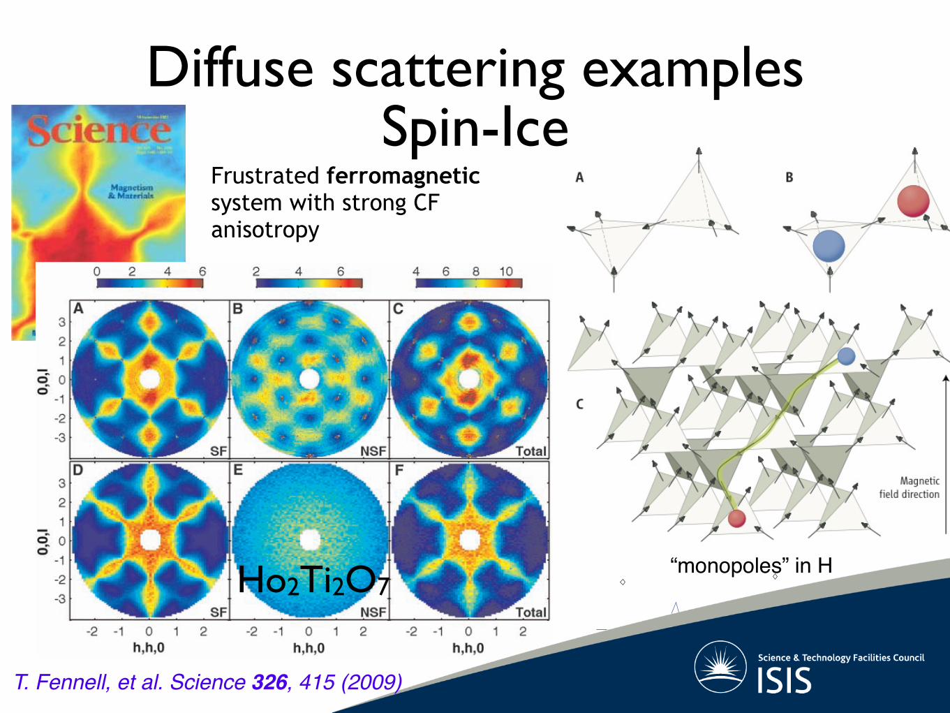
Fig. 2. Diffuse scattering maps from spin ice, Ho2Ti2O7. Experiment [(A) to (C)] versus theory [(D) to(F)]. (A) Experimental SF scattering at T = 1.7 K with pinch points at (0, 0, 2), (1, 1, 1), (2, 2, 2), and soon. (B) The NSF scattering. (C) The sum, as would be observed in an unpolarized experiment (20, 22).(D) The SF scattering obtained from Monte Carlo simulations of the near-neighbor model, scaled tomatch the experimental data. (E) The calculated NSF scattering. (F) The total scattering of the near-neighbor spin ice model.
0 1 2 3 40
2
4
6
!"
0,0,l
1.7 K
NSFSF
0
2
4
6
!"
1.7 K
TotalNSFSF
0
2
4
6
Inte
nsity
(a.u
.)
1.7 K
NSFSF
!0.6 !0.3 0 0.3 0.60
2
h,h,2
!"
50 K20 K10 K5 K3.75 K2.5 K1.7 K
A
B
C
D
Fig. 3. Line shape of the pinch point. (A) Radialscan on D7 through the pinch point at (0, 0, 2)[s! is the neutron scattering cross section; see (26)for its precise definition]. (B) The correspondingtransverse scan. The lines are Lorentzian fits. (C)Higher-resolution data, in which the line is aresolution-corrected fit to the pinch point form Eq.1 (the resolution width of the spectrometer is indi-cated as the central Gaussian). (D) SF scattering atincreasing temperatures (the lines are Lorentzianson a background proportional to the Ho3+ formfactor).
16 OCTOBER 2009 VOL 326 SCIENCE www.sciencemag.org416
REPORTS
on
Nov
embe
r 5, 2
009
ww
w.s
cien
cem
ag.o
rgD
ownl
oade
d fro
m
Diffuse scattering examples
Ho2Ti2O7
T. Fennell, et al. Science 326, 415 (2009)
“monopoles” in H
Spin-IceFrustrated ferromagnetic system with strong CF anisotropy

Polymer diffraction
Complete separation of SI scattering
Internal normalisation (inc. D-W factor)
Careful analysis of multiple scattering
Close comparison with MD simulations
Polyisoprene: (CH2CH = C(CH3)CH2)n
Alvarez, et. al.PI-h8
PI-d5
PI-d3
PI-d8
Q (Å-1)
Alvarez, et.al., Macromolecules 36 (2003) 238

Inelastic magnetic scattering
Rule, et. al., Phys. Rev. B 76 212405 (2007)
Pyrochlore - Tb2Sn2O7

Science with Polarized Neutrons
Magnetic slow-relaxation in “spin-ice”
Ehlers et al, J Phys: Condens Matter 18, R231 (2006)
S(Q
,t)/
S(Q
,0)
Glass transition in polymer-glass, polybutadiene
A. Arbe et al Phys. Rev. E 54, 3853 (1996)
S(Q
,t)/
S(Q
,0)