November 2003

Polarization microscopy with the LC-PolScope

Rudolf OldenbourgMarine Biological Laboratory, Woods Hole, MA 02543, USA

Rudolf OldenbourgMarine Biological Laboratory7 MBL StreetWoods Hole, MA 02543, USATel: 508-289-7426Fax: 508-540-6902e-mail: rudolfo@mbl.edu

Table of Contents

Introduction ................................................................................................................................2Instrumentation...........................................................................................................................4

Basic optical set-up .................................................................................................................4Design specifics and variances ................................................................................................6

Polarization optical components ..........................................................................................6Choice of optics ..................................................................................................................8Inverted microscope stand...................................................................................................9Culture chamber and heating stage ....................................................................................10Choice of light source .......................................................................................................10Combining the PolScope with DIC and fluorescence imaging ...........................................11Specimen preparation........................................................................................................13

Image acquisition and measurement..........................................................................................14Calibration ............................................................................................................................14Retardance measurement.......................................................................................................15Background birefringence and how to correct it ....................................................................16

Performance characteristics and how to measure them ..............................................................19Resolution.............................................................................................................................19Sensitivity and noise sources.................................................................................................21Accuracy...............................................................................................................................23Speed ....................................................................................................................................24And use the Bertrand lens .....................................................................................................25

Example Images and Movies ....................................................................................................25Glossary of polarization optical terms .......................................................................................26Acknowledgments ....................................................................................................................30References ................................................................................................................................30Figures......................................................................................................................................33

2

IntroductionMost of the imaging approaches discussed in this Lab Manual are based on the use of fluo-

rescent molecules and their detection inside living cells. Only a decade ago, live cell imagingwas dominated by techniques such as phase contrast, differential interference contrast and po-larized light microscopy which do not require the introduction of exogenous dyes or markers.Fluorescence microscopy, on the other hand, often required the killing and fixation of cells andthen labeling them to detect specific molecular species. This role reversal was made possible bythe many spectacular advances in fluorescence imaging and the development of many vital mo-lecular probes, particularly the green fluorescent protein, which have seemingly outshined themore traditional techniques which probe the subtle changes of phase and amplitude of light thathas interacted with the specimen. The phase sensitive techniques create images of living cellsbased on their intrinsic optical properties, in particular their refractive index. While the limelightwas on fluorescence imaging, the more traditional techniques for live cell imaging have madegreat gains as well and they remain indispensable as complementary tools for imaging cellstructure and function without the need for introducing fluorescent molecules into cells (Inouéand Spring, 1997; Sluder and Wolf, 1998).

Polarization microscopy uses polarized light to probe the local anisotropy of the specimenoptical properties, such as birefringence or dichroism. These optical properties, which we willdiscuss in more detail later, have their origin in molecular order, i.e. in the alignment of molecu-lar bonds or fine structural form in the specimen. Hence, polarization microscopy providesstructural information at a submicroscopic level, including the alignment of molecules in fila-ment arrays and membrane stacks such as the mitotic spindle, f-actin arrays, and retinal rod outersegments. Therefore, the polarizing microscope not only gives us information about where andwhen certain structures form and change inside the living cell, but also some of the submicro-scopic features of these structures. Most importantly for live cell imaging, the polarizing micro-scope can do so dynamically both in short and long time periods, at the highest resolution of thelight microscope, and with minimal interference with the physiological conditions required forthe maintenance of live and healthy cells.

The use of the polarizing microscope for studying living cells was pioneered more than 70years ago by W. J. Schmidt whose many original observations were published in a celebratedmonograph (Schmidt, 1937). Intrigued by Schmidt’s observations and Ambronn and Frey(Ambronn and Frey, 1926), and Frey-Wyssling studies (Frey-Wyssling, 1953), other groups be-gan to use and refine the technique for live cell imaging, in particular for the phenomenon of celldivision (Inoué, 1952; Inoué, 1953; Inoué and Dan, 1951; Inoué and Hyde, 1957; Mitchison,1950; Swann and Mitchison, 1950), for a recent review of polarized light microscopy of spindlessee (Oldenbourg, 1999)). For a discussion of the traditional polarized light microscope and itsmany uses in cell biology, the reader is referred to a recent article by Shinya Inoué, who for morethan 50 years is the technique’s strongest proponent ((Inoué, 2002), see also Appendix III in thefirst edition of (Inoué, 1986)).

In the current chapter we describe the use of a new type of polarized light microscope whichwe started to develop at the Marine Biological Laboratory about ten years ago. The new “Pol-Scope” is based on the traditional polarized light microscope and enhances it with the use of liq-uid-crystal devices and special image processing algorithms. The LC-PolScope measures polari-zation optical parameters in many specimen points simultaneously, in fast time intervals, and at

3

the highest resolution of the light microscope. It rapidly generates a birefringence map whosepixel brightness is directly proportional to the local optical anisotropy, unaffected by the speci-men orientation in the plane of view, as well as a map depicting the slow axis orientation of thebirefringent regions. The basic LC-PolScope technology can be adapted to most research grademicroscopes and is available commercially from Cambridge Research and Instrumentation (CRI,http://www.cri-inc.com) in Woburn, Massachusetts, under the trade name LC-PolScope.

The advantage of the LC-PolScope over the traditional polarizing microscope rests in itsspeed, sensitivity and accuracy. As Shinya Inoué likes to point out, for a seminal study on DNAorganization in sperm heads it took him and two colleagues three years to analyze the polarizedlight images of three living cave cricket sperm (Inoué and Sato, 1966). A similar analysis wouldtake seconds using the LC-PolScope. It must be said that the LC-PolScope measures specimenproperties that, in principle, can be measured with the traditional polarizing microscope. How-ever, the vastly improved speed and completeness of measurement (birefringence parameters forall resolved specimen points simultaneously) make the LC-PolScope the instrument of choice formany studies that benefit of the analytic power and submicroscopic information gleaned frompolarized light images. Nevertheless, in some cases the traditional polarizing microscope mightsuffice to provide the needed information, be it the organization of filaments, membranes orchromophores in living cells (see the aforementioned article by (Inoué, 2002)). The decision touse the LC-PolScope is sometimes based on observations with the traditional instrument. Insome cases one can find relevant information in the literature (see for example the extensive bib-liography in Appendix III in the first edition of (Inoué, 1986)), other times one might do the ex-ploratory observations using the traditional instrument oneself. This chapter was written for ex-perimental scientists who want to get a better understanding of the capabilities of the new in-strument and those who wish to optimize their use of it.

In describing the use of the LC-PolScope for live cell imaging, we first discuss the basic in-strument, including the optical, electronic and software components and the influence of theirperformance parameters on the sensitivity, resolution, and speed of LC-PolScope measurements.As with the traditional polarizing microscope, the LC-PolScope technology can be implementedusing many different design variations either for adapting it to a special measurement set-up, forimproving the performance of the instrument or for measuring different optical parameters in thespecimen. In describing the design we included some of these design variations which can beimplemented with a few modifications to the basic PolScope instrument. We continue the discus-sion with the description of the image acquisition and measurement procedures used in the LC-PolScope, and of its performance characteristics and how to measure them. A good understand-ing of these issues puts the experimenter in a better position for optimizing the performance ofthe instrument for the specific study at hand. Towards the end we present a number of LC-PolScope images of living cells to give examples of the current range of systems studied withthis new incarnation of an old and powerful technique.

Throughout this chapter we will use polarization optical terms such as retardance and opticaxis which might not be familiar to the reader. Therefore, at the end we compiled a glossary ofpolarization optical terms, including a brief outline of the optical concepts of birefringence andretardance and of their measurement using imaging optics.

We believe the LC-PolScope technology is only at the beginning of a bright future. In ourown laboratory at the MBL and in collaboration with CRI we continue to advance the LC-PolScope technology. We are working on extending its measurement capabilities beyond bire-

4

fringence, including dichroism and fluorescence polarization. Especially for improving live cellimaging we are working on increasing the speed of measurement to reduce the possibility of im-age artifacts due to specimen movements. We are also developing methods to measure polariza-tion optical parameters in 3-dimensions. Hand in hand with these advances in instrumentation weare developing analytical tools for the interpretation of image content and for image restoration.All these developments are aimed to further unlock the secrets of cell structure and function asdisplayed in the architectural dynamics in living cells (for updates on our activities seehttp://www.mbl.edu/research/resident/lab_oldenbourg.html).

InstrumentationThe LC-PolScope instrumentation includes optical and electronic components and software

for image processing and analysis. We first discuss general considerations regarding the opticalset-up and strategies for selecting optical components for achieving best results. We also discussconsiderations for combining PolScope optical elements with other imaging modalities, notablydifferential interference contrast (DIC) and fluorescence imaging. Finally, the specimen can beconsidered one of the optical components. Therefore, we give a few guidelines for preparingspecimens and specimen chambers that are suitable, or incompatible, for observations with po-larized light.

The LC-PolScope technology discussed in this chapter is covered by a US patent(Oldenbourg and Mei, 1996) which is licensed to Cambridge Research and Instrumentation(CRI) in Woburn, Massachusetts, USA (http://.cri-inc.com). CRI developed a commercial ver-sion for cell biology under the trade name LC-PolScope. The LC-PolScope includes opticalcomponents that are inserted into a microscope stand. Most stands from major microscope manu-factures are suitable and can be optimized using the guidelines discussed in this chapter. Wehave prepared our instrumentation guidelines with the commercial version of the LC-PolScope inmind. We also discuss design variations that can be considered by the more experienced user ofthe LC-PolScope equipment, sometimes in collaboration with CRI, which is committed to sup-porting their customers in new and unconventional uses of the instrument. Furthermore, the LC-PolScope technology is constantly expanded and improved upon by CRI and by our own re-search at the Marine Biological Laboratory.

Basic optical set-up

The optical design of the LC-PolScope builds on the traditional polarized light microscopeintroducing two essential modifications: the specimen is illuminated with nearly circularly po-larized light and the traditional compensator is replaced by an electro-optic, universal compen-sator. The PolScope also requires the use of monochromatic light. In Figure 1, the schematic ofthe optical train shows the universal compensator located between the monochromatic lightsource (e.g. arc lamp with interference filter) and the condenser lens. The analyzer for circularlypolarized light is placed after the objective lens. The universal compensator is built from twovariable retarder plates and a linear polarizer (see text box The Universal Compensator).The variable retarder plates are implemented as electro-optical devices made from two liquidcrystal plates. Each liquid crystal plate has a uniform retardance that depends on the voltage ap-plied to the device. The voltage for each plate is supplied by an electronic controller box con-nected to the retarders. The retarder controller box includes a microprocessor that stores liquidcrystal related parameters for control of the variable retarder plates. The controller box is

5

The Universal Compensator

The universal compensator is built from two liquid crystal devices LC-A and LC-B, each ofwhich functions as a uniform linear retarder plate. The retardance of a single plate can be ad-justed between about 50 nm and 800 nm by applying a voltage between 10 Volt (800 nm) and40 Volt (50 nm) to the liquid crystal device (for a more detailed description of liquid crystal vari-able retarders see (Khoo and Wu, 1993)). When changing the voltage, only the retardancechanges, while the orientation of the slow (or fast) birefringence axis remains fixed.

As indicated in Figure 1, the slow axes of the linear retarders are mutually oriented at 45° toeach other. In addition, the universal compensator includes a linear sheet polarizer (polar)whose transmission axis is oriented at 45° to the slow axis of LC-A. The polarizer and two liquidcrystal plates are bonded together to form a thin optical flat with antireflection coatings on eachside. The clear aperture can be 25 mm and larger and the stack is about 6 mm thick.

For measuring polarization optical properties of a specimen, the opticalset-up also includes a circular polarizer. As indicated in Figure 1 and tothe right here, a circular polarizer is typically built as a sequence of a lin-ear sheet polarizer and a fixed quarter wave plate.

There are two basic choices for adding the universal compensator to themicroscope optical train: Either before the condenser lens (case 1 on theright, also shown in Figure 1), or after the objective lens (case 2). In bothcases, the specimen (and high numerical aperture optics) is sandwichedbetween the universal compensator and the circular polarizer. Further-more, the wave plates (the quarter wave plate of the circular polarizerand the LC wave plates of the universal compensator) are facing thespecimen. Or, in other words, in both cases the linear polarizers are thefirst and last elements in the polarization optical train.

Hence, in either case, the specimen, high NA optics, and fixed and vari-able retarder plates are forming a polarization optical train sandwichedbetween two linear polarizers. This polarization optical train can be ana-lyzed using mathematical descriptions known as Müller matrices andStokes vectors. Based on such an analysis, we have developed imageacquisition procedures and algorithms that allow one to use thePolScope for measuring polarization optical properties of the specimenin every resolved image point simultaneously (see Retardance meas-urement).

Both arrangements are equivalent in their ability to measure polarizationoptical parameters of the specimen. For the optical purist, though, case1 might be preferable to case 2 which adds the universal compensatorto the imaging path between objective and camera. Compared to the cir-cular polarizer, the universal compensator represents a thicker opticalflat and therefore might compromise the performance of the highly cor-rected objective lens. In practice, however, in most cases this differenceis negligible.

Some additional optical properties, performance parameters and possi-ble modifications to the universal compensator and circular polarizer arediscussed under Polarization optical components and through out thischapter.

univ

ersa

lco

mpe

nsat

orci

rcul

arpo

lariz

er

LC-A

LC-B

polar

case 1

univ

ersa

lco

mpe

nsat

or

LC-A

LC-B

polar

case 2

circ

ular

pola

rizer

6

connected to a desk-top computer using a serial interface. The desk-top computer is also con-nected to the electronic camera, typically a CCD camera (charge coupled device), for recordingthe specimen images through the microscope optics. Specific software in the desk-top computeris designed to synchronize the image acquisition process with the liquid crystal control and toimplement image processing algorithms that compute images representing the retardance andprincipal axis orientation in every resolved image point.

We want to emphasize, that during recordings of all four images in Figure 1, no part of themicroscope set-up, including the specimen, was mechanically moved. To obtain the four images,only the voltages applied to the liquid crystal devices were changed. Therefore, all four imagesrecorded with the CCD camera are in perfect register, with corresponding picture elements repre-senting intensities of the same object elements. Optimal image registration is particularly impor-tant for measurements requiring high spatial resolution.

Design specifics and variances

Polarization optical components

Polarizers: The linear polarizers used in a PolScope should have high transmission and goodextinction. Modern sheet polarizers are now available with transmission coefficients for unpo-larized light of higher than 40% and extinction coefficients of around 104. An ideal polarizer hasa transmission of 50% and infinite extinction. The extinction is a measure of the purity of thepolarization state of light, after it has passed through the polarizer. The extinction coefficient ismeasured by the ratio of light transmitted through two polarizers in sequence, with their trans-mission axes aligned either parallel or perpendicular to each other (extinction = I|| / I^). Glan-Thompson and other prism polarizers perform close to the ideal values. For reasons given belowgood sheet polarizers are typically sufficient for the LC-PolScope.

The purity of the polarization in a light microscope is usually limited by the polarizationdistortions introduced by high numerical aperture condenser and objective lenses. While a pair ofsheet polarizers might have an extinction ratio of 104 or higher, if a condenser and objective lensis placed between them, the extinction usually drops to around 103 or below (a pair of 1.4 NA oilimmersion condenser and objective lenses has an extinction coefficient of around 200 if the con-denser aperture diaphragm is fully open; partially closing the condenser aperture increases theextinction). Due to the development of calibration and correction procedures for the LC-PolScope, extinction plays a less critical role in the PolScope than in a traditional polarizing mi-croscope. However, the sensitivity for measuring small retardance values that might be below0.01 nm can be limited by the extinction of the set-up (see Performance characteristics

and how to measure them). In the following section, Choice of optics, we discuss theproper choice of lenses and refer to articles discussing the use of polarization rectifiers to mini-mize polarization distortions in high numerical aperture systems and optimize the performance ofthe LC-PolScope.

The circular polarizer used in the LC-PolScope is usually assembled from a linear polarizerand a quarter wave plate (see text box: The Universal compensator). Both components aremade of thin polymer sheets of high optical quality that are bonded together. When inserting thecircular polarizer in the optical path, care must be taken to insert it right side up. As illustrated inthe text box The Universal compensator, the correct orientation depends on the arrange-ments illustrated in case 1 and case 2. In either case, the quarter wave plate of the circular po-

7

larizer faces the specimen. For testing which side the quarter wave plate is on, one can use aseparate linear polarizer. Looking through the circular and linear polarizer in tandem against awhite light source, one rotates the two devices about their common normal axis and checks forextinction. Good extinction can only be achieved if the quarter wave plate is located outside thepath between the two linear polarizers. If, however, the quarter wave plate is between the twolinear polarizers, then different rotation angles result in differently colored light, but no extinc-tion can be achieved.

While it matters to insert the circular polarizer right side up in the LC-PolScope optical train,it does not matter how it is rotated around the optical axis of the microscope. This is in starkcontrast to a traditional polarizing microscope using linear polarizers which have to be carefullyrotated to their crossed position. We leave it to the reader as an exercise to find an explanationfor this peculiar feature of the LC-PolScope arrangement.

In a LC-PolScope with a straight optical path the circular polarizer usually transmits left cir-cularly polarized light and absorbs right circularly polarized light. In some microscopes a mirroris present in the optical path between universal compensator and circular polarizer. Upon reflec-tion by a mirror, circularly polarized light changes handedness. Therefore, in such a microscopethe circular polarizer that is usually used in the LC-PolScope needs to be exchanged against onethat transmits circularly polarized light of the opposite handedness. An even better solution is torearrange the polarization elements in such a way that no mirror is in the optical path betweenthem; because mirrors, like lenses, usually introduce polarization aberrations and reduce the ex-tinction of the set-up.

Finally, we note that the circular polarizer is typically made for a specific wavelength, unlessthe quarter wave plate is specified for a range of wavelengths, a so-called achromatic quarterwave plate. If frequent changes between two or more wavelengths are necessary, one might con-sider using such an achromatic circular polarizer or obtain a tunable circular polarizer made, forexample, of a linear polarizer and a liquid crystal variable retarder.

Universal compensator: The universal compensator is manufactured by Cambridge Researchand Instrumentation and is made of two liquid crystal variable retarders and a linear polarizer(see text box: The Universal compensator). These components are usually bonded togetherand we assess their polarization optical performance as a unit. When considering the universalcompensator as a unit by itself, it can also be called a variable polarizer based on the followingproperty. When shining monochromatic light through the device so the light first passes throughthe linear polarizer followed by the two variable retarders, the light leaving the retarders can bemade to have any desired polarization state, be it linear polarization of any azimuth or ellipticalpolarization of any handedness, ellipticity or azimuth (see equations 2,3,and 4 in (Shribak andOldenbourg, 2003)). When shining light through the device in the opposite direction, so it firstpasses through the variable retarders and then through the linear polarizer, the device functionsas a universal polarization analyzer. In this configuration extinction can be achieved for any in-put polarization by setting the retardance of the liquid crystal variable retarder plates to suitablevalues. Based on the retardance values needed for extinction, one can calculate the polarizationof the incoming light using equations that are equivalent to the ones referred to earlier. Thisproperty can be used for some unconventional applications of the universal compensator. Forexample in fluorescence imaging, when inserting the universal compensator in the illuminationpath or imaging path (or both) the specimen can be illuminated with light of a specific polariza-tion and/or the light from the specimen can be analyzed for any given polarization state.

8

With regard to the performance of the universal compensator, we give instructions on how tomeasure the extinction coefficient of the complete PolScope optical set-up in the section Per-

formance characteristics and how to measure them.

Apart from extinction and transmission, another important performance parameter of the uni-versal compensator is the time required to reliably switch between two polarization states, the so-called settling time. The settling time is determined by the liquid crystal devices and is usuallygreater than 100 ms. However, faster settling times are possible and LC devices can be con-structed with settling times of 30 ms and lower, usually at the expense of the range of retardancevalues that the devices can be adjusted to.

Choice of optics

As indicated earlier, the polarization distortions introduced by the objective and condenserlenses limit the extinction that can be achieved in a polarizing microscope. But not all lenses arecreated equal. Most microscope manufacturers offer lenses that are designated “Pol” to indicatelow polarization distortions which can arise from a number of factors, including stress or crys-talline inclusions in the lens glass and the type of antireflection coatings used on lens surfaces.Some lens types are not available with “Pol” designation, but with the designation “DIC”. Theselenses don’t measure up to the more stringent Pol requirements but pass for the use of differentialinterference contrast and can also be used with the LC-PolScope (without the special Wollastonor Nomarski prisms, of course).

The polarization performance of the most highly corrected lenses, so called Plan Apochromatobjectives, is often compromised due to the large number of lens elements, the specialantireflection coatings, and in some cases the special types of glass used to construct the lenses(Inoué and Oldenbourg, 1995). For some applications of the LC-PolScope the Plan-Apochromatcorrection might be overkill anyway. If you plan to use the objective lens only with the PolScopethat requires monochromatic light and typically acquires images from a region near the center ofthe viewing field, a correction lesser than Plan Apochromat might suffice. The special lens de-sign for Plan Apochromats providing a large, highly corrected viewing field over a wide spectralrange is often not required for LC-PolScope applications. To find out what works best for a par-ticular imaging situation, we recommend to test a few lenses. For best performance, it is alsohelpful to be able to select the best performing pair of condenser and objective lens from a batchof the same lens types.

Whenever possible or practical, use oil immersion lenses. Oil, and to a lesser degree waterand other immersion liquids, greatly reduce polarization aberrations caused by air-glass inter-faces between the specimen and the lenses. The transition of a light ray between two media ofdifferent refractive index (nair = 1.00, nglass = 1.52) introduces polarization distortions, especiallyfor high NA lenses. The peripheral rays leaving the condenser front lens are highly tilted to theslide surface and their polarization is typically rotated when traversing the air-glass interface(Inoué, 1952; Inoué and Hyde, 1957). For a discussion of the origin of polarization distortions inlenses and optical systems and of ways to reduce them we refer to a recent article by Shribak etal. (Shribak et al., 2002). The publication also discusses the various conoscopic images that canbe observed in a polarizing microscope equipped with crossed, or nearly crossed polarizers and aBertrand lens.

9

Lenses and other optical elements that are not placed between the universal compensator andthe circular polarizer do not affect the extinction performance of the microscope set-up. There-fore, in a dissecting microscope for example, the polarizing elements and the liquid crystal de-vices might be better placed between the objective lens and the light source. The light source istypically an incandescent lamp with diffuser plate in the base of the dissecting scope. On top ofthe diffuser plate one can first place an interference filter followed by the fixed circular polarizer.The liquid crystals might be mounted in a special holder in front of the objective lens. In a dis-secting microscope, the rays captured by the objective to project the image have small tilt angles(low NA). Hence, the rays passing through the liquid crystals have small enough tilt angles asnot to compromise the polarization performance of the liquid crystals.

While optical elements placed outside the polarization optical train don’t affect the extinc-tion, they do contribute to the overall performance of the set-up. Aside from considerations re-garding image quality, the sensitivity of measuring small retardance features in the specimen alsodepends on the proper match between the resolution of the optical image and of the electroniccamera. We will address the relationship between resolution, sensitivity and speed of measure-ment in the section on Performance characteristics and how to measure them.

Inverted microscope stand

Inverted stands equipped with the required optical components can be equally suited for po-larized light microscopy as upright stands. Here are a few points to consider when using an in-verted stand for the PolScope:

• Inverted stands frequently have a mirror in the optical path. A mirror has two effects:(1) the circular polarizer or analyzer might have to be exchanged for one with the op-posite handedness, because circularly or elliptically polarized light changes handed-ness upon reflection by a mirror (only relevant if the mirror is in polarization opticalpath, between the universal compensator and the analyzer);(2) if the mirror is in the imaging path, the calculated azimuth angle needs to be in-verted because of the change in symmetry of the raw LC-PolScope images. Acheckbox named “Inverted microscope” is provided in the LC-PolScope software toinclude this final inversion step. If one failed to check the box and needs to correctthe angle later, simply replace the old azimuth value j by (180°-j) .

• Plastic Petri-dishes, often used with inverted scopes, cannot be used with thePolScope. However, plastic Petri-dishes with a glass bottom are ok (see, for example,http://www.glass-bottom-dishes.com/).

• If your cell preparation is in a culture dish with a glass bottom, you might considertrans-illuminating your specimen using an immersion condenser that dips into theaqueous culture medium. A water immersable objective as condenser lens will givebest results, but requires modifications to the condenser mounting. As an alternative,a regular oil immersion condenser can be dipped into the medium to avoid the airglass and air water interface and the concomitant polarization distortions of a drycondenser lens. It also provides for high NA illumination for improved resolution. Ofcourse, in the process the sterility of the culture will be compromised. Also, oneshould carefully wipe the condenser dry after contacting it with an aqueous medium.

10

Culture chamber and heating stage

For a comprehensive discussion on culture chambers, heating stages and other accessories forkeeping live cells happy while they are mounted on the microscope we refer to the special chap-

ters in this Lab Manual. For observations using polarized light we want to point out the fol-lowing issues:

• Absolutely avoid plastic components in the polarization optical path. Most plasticmaterials are highly birefringent and therefore greatly reduce the sensitivity and accu-racy of the LC-PolScope measurement. In some cases it is possible to replace theplastic material with suitable glass components A case in point is the modified plasticPetri dish with glass bottom.

• Avoid equipment that introduces temperature gradients in objective and condenserlenses and in other optical components that are part of the polarization optical train ofthe microscope. Temperature gradients in glass cause stress and associated stress bire-fringence which reduces the sensitivity of the PolScope. Stress birefringence also in-troduces a background retardance that usually changes over time, modulating thecalibration of the instrument.

Choice of light source

The PolScope requires a stable, bright, monochromatic light source. Depending on the appli-cation, the requirements can be met by a halogen lamp, an arc lamp (e.g. mercury or xenon), alight emitting diode (LED) or suitably scrambled laser light. For a more detailed discussion oflight sources for live cell imaging we refer the reader to the chapter by Phong Tran in this Lab

Manual. Here we briefly discuss the effect of different lamp characteristics on PolScope meas-urements.

Stability is paramount among the specifications for a light source suitable for the PolScope.The lamp intensity must be stable during the time period required for the exposure of a stack ofraw PolScope images. For example, for measuring retardance values of around 0.1 nm using astandard LC-PolScope optimized for low retardance measurments, the lamp intensity must bestable within 1%. An unstable light source is tantamount to varying the exposure level betweenraw PolScope images which in turn has the same effect as introducing a uniformly birefringentplate in the polarization optical train. However, in some cases, PolScope images that were ex-posed using an unstable light source can be corrected after the fact using the background ratioingmethod discussed below under Background birefringence and how to correct it.

Brightness is another important factor to consider in polarization microscopy. Obviously, theintensity of the light source is directly proportional to the time it takes to expose the camera de-tector to appropriate light levels. Furthermore, for measuring small retardance values, thePolScope is operated with settings of the universal compensator that are near extinction. Hence,the light level on the camera and in the eye piece for direct observations are low and it can be-come difficult to align the instrument and position and focus the sample correctly without suffi-cient light. Therefore, a bright light source is needed for an efficient work flow, especially whenworking with live cells. Since cells are sensitive to light the PolScope set-up should include ashutter that is conveniently operated and blocks the light to the specimen whenever possible.Blocking the light when it is not needed is an efficient way of reducing light damage to the cells.

11

The PolScope requires monochromatic light for its operation. Light with a spectral band-width of 30 nm is an upper limit and should not be exceeded without risking to loose sensitivity(increased spectral width reduces the extinction of the set-up). Therefore, most light sources, ex-cept for lasers, require an interference filter for selecting or narrowing the spectral range of thesource. In contrast, a laser’s spectral width is usually too narrow and its time coherence too longfor wide field imaging (Inoué and Spring, 1997).

In our own experience, a 100W mercury arc lamp, as supplied by microscope manufacturersand equipped with a 546 nm interference filter (http://www.omegafilters.com orhttp://www.chroma.com), provides sufficiently bright, monochromatic light for measuring fast,dynamic events, such as spindle dynamics during mitosis. Other strong emission lines of a mer-cury arc lamp have center wavelengths of 577 nm and 436 nm and can also be used after ex-changing the interference filter and circular polarizer suitable for the selected wavelength. Typi-cally, when an arc burner is used longer than 150 hours, the gap between the electrodes increasesand the shape of the tip of the electrodes often becomes irregular leading to an instable arc ge-ometry. As a result, the brightness of the lamp starts to flicker. When lamp flickers become ap-parent by direct viewing, or the flickers can be recognized as elevated background retardancethat changes erratically over time (see above), it is probably time to change the bulb. To improveresolution and minimize image artifacts we also use a fiber based Ellis light scrambler which isavailable from Technical Video, Ltd (http://www.technicalvideo.com/). Finally, there are severalways to adjust the amount of light delivered to the specimen, including a diaphragm that variesthe light level entering the fiber optic light scrambler, and neutral density filters with calibratedattenuation factors. Avoid closing the condenser aperture to reduce the light level, because thiswill also decrease the resolution of the image.

In the future we expect light emitting diodes (LEDs) to replace traditional light sources formany applications, especially when monochromatic light is needed. Over the past several years,LEDs have improved significantly with respect to their brightness and now can provide higherintensity monochromatic light compared to halogen lamps. LEDs are highly efficient and stablelight sources, whose brightness can be controlled by the source current. They can also be drivento provide short light pulses with peak powers that are several times the DC power limit (see forexample http://.lumileds.com).

Combining the PolScope with DIC and fluorescence imaging

For differential interference contrast (DIC), two matching prisms are added to the polariza-tion optical path (for a discussion of the standard DIC arrangement see (Salmon and Tran,1998)). The two prisms, called Wollaston or Nomarski prisms, are specially designed to fit inspecific positions, one before the condenser and the other after the objective lens, and to matchspecific lens combinations. The prisms in their regular positions can be combined with thePolScope set-up, in which case the universal compensator and circular analyzer take the placesof the linear polarizer and analyzer in a standard DIC arrangement. In fact, the same DIC prismsfunction equally well using either linearly or circularly polarized light.

For best results, the PolScope is first calibrated without prisms to find the extinction settingfor the universal compensator. With the compensator set to extinction, the prisms are entered intothe optical path. Typically, one of the two prisms has a mechanism for fine-adjusting its positionwhich in turn affects the brightness and contrast of the DIC image. In a PolScope set-up, one caneither use the mechanical fine adjustment or one can use the universal compensator to add a bias

12

retardance to change the brightness and contrast of the DIC image. When using the universalcompensator, one needs to add or subtract retardance from the extinction setting of either theLC-A or LC-B retarder (see Figure 1), depending on the orientation of the shear direction of theprisms.

For live cell imaging, we find it very useful to switch easily between PolScope and DIC im-aging. DIC provides good contrast of many morphological features in cells using direct viewingthrough the eye piece or by video imaging. When viewing specimens that have low polarizationcontrast, we find it more effective to align the optics including the visualization of the specimenusing DIC. After the optics are aligned and the specimen is in focus, the DIC prisms are removedfrom the optical path and the PolScope specific adjustments are completed.

Fluorescence imaging can be combined with the PolScope in several ways. Fluorescence iscommonly observed using epi-illumination requiring a filter cube in the imaging path. The filtercube includes a dichromatic mirror and interference filters for separating the excitation and emis-sion wavelengths. For best results the filter cube should be removed for PolScope observations toavoid the polarization distortions caused by the dichromatic mirror. For observing fluorescence,on the other hand, the PolScope analyzer should be removed, because it attenuates the fluores-cence emission by at least 50%. To meet both requirements one can mount the PolScope ana-lyzer in an otherwise empty filter cube holder which is moved into the optical path as the fluo-rescence cube is moved out, and vice versa.

If, however, the option of removing the fluorescence cube is unavailable, the cube can re-main in the optical path for PolScope observations. In this case, consider the following points:

• For the light source of the PolScope choose a wavelength that is compatible with theemission wavelength filter in the fluorescence cube. For example, fluorescein isothio-cyanate (FITC) requires excitation with blue light (485 nm) and fluoresces in thegreen. The FITC dichromatic beam splitter and barrier filter passing green fluores-cence light with wavelength longer than 510 nm would be compatible with 546 nmlight for PolScope observations using a mercury arc burner for the transmission lightpath.

• Calibrate the PolScope with the fluorescence filter cube in place. The polarizationdistortions caused by the dichromatic mirror are partially counteracted by the cali-brated settings of the universal compensator.

• Make sure the light source for one imaging mode is blocked while observing with theother imaging mode.

• Removing the PolScope analyzer while observing fluorescence more than doubles thefluorescence intensity.

While beyond the scope of this article, it should be noted that the universal compensator canalso be used to analyze fluorescence polarization. As described in the section on Polarization

optical components, the universal compensator can also be regarded as a universal polariza-tion analyzer or a universal polarizer. It can thus play a valuable role in selectively exciting ordetecting polarized fluorescence. Fluorescence polarization imaging has become a powerful toolfor probing structure together with functional aspects in living cells and working model systems.Fluorescence polarization can be used as binding assay of small and medium-sized molecules toreceptors and other binding sites. (Peterman et al., 2001) and as probe to differentiate between

13

conformational states (Warshaw et al., 1998). The combination of molecular specificity and dy-namic measurement of molecular orientation by fluorescence polarization analysis has revealedthe rotational motion of actin filaments during sliding over myosin molecules fixed on a glasssurface (Sase et al., 1997). Recently, Inoué and colleagues have discovered and analyzed the re-markable fluorescence polarization properties of single crystals of the green fluorescent protein(Inoué et al., 2002). As indicated in this paper, the highly polarized nature of GFP fluorescenceprovides a new method for dynamically observing, and quantifying, the changing orientation offluorescent chromophores constituting (or attached to) functional molecular structures.

Specimen preparation

Last, but certainly not least, we consider the specimen and its mount as part of the polariza-tion optical train. There are several chapters in this Lab Manual which discuss the preparationof viable cells suitable for observations in the light microscope. We also refer to the recent articleby Shinya Inoué on polarized light microscopy in a Lab Manual for Cell Biology (Inoué, 2002).Also, our article on polarized light microscopy of spindles has a section on cell types suitable forlive cell imaging of spindles and their preparation (Oldenbourg, 1999). Here we will give a fewgeneral pointers for making live cell preparations for the PolScope.

• Prepare the specimen so that when mounted in the microscope you can identify atleast one clear area without cells or birefringent material and move it into the viewingfield when required. A clear area is needed for calibrating the PolScope and for re-cording a PolScope stack of background images. The background images provide arecord of the combined effect of the polarization properties of all optical components,including the slide and coverslip, but not of the specimen itsself. Using the back-ground images, the spurious background retardance is removed from PolScope im-ages of the cells and structures that you wish to measure precisely and image clearly.Many cell cultures or cell free systems are suitably prepared without special attentionto this requirement. For example, a free area can often be found around cells that aresparsely plated on coverslips. Cultures of free swimming cells might have to be di-luted appropriately before mounting a small drop between slide and coverslip. Some-times we find it helpful to add a tiny drop of oil or other non-toxic, immiscible liquidto the preparation. The clear drop can provide an area for calibrating the instrumentand take background images in a preparation that is otherwise dense with birefringentstructures. For further discussions on collecting background images see Back-

ground birefringence and how to correct it and Performance characteris-

tics and how to measure them.

• If your cells are round and small, the edge birefringence of the cell surface might bestrong and obscure other detail. For reducing the edge birefringence you can add,polyethyleneglycol, polyvinylpyrrolidone, or some other harmless polymer or proteinsubstitute to increase the medium’s refractive index. The percent concentration ofsubstitute required might vary from a few percent to 16% and more, depending on theaverage refractive index of the cytoplasm of the cells you are studying. It is best tomake up a few trial solutions of media with different polymer concentrations, suspendthe cells in them and look at a slide and coverslip prep with DIC or polarized light. Atthe right polymer concentration, the cells will look as if their internal organelles andcytoskeleton are suspended in space because you can see no distinct cell boundary.

14

After determining the concentration you should test the compatibility by growingcells in medium with polymer. Cells should grow and develop normally in media withthese types of additives. The molecular weight of the polymer should be around 40kD or more to prevent its uptake into cells.

• Earlier in this chapter, we recommended the use of immersion optics whenever possi-ble (see Choice of optics). When using high NA oil immersion optics, preparespecimens in which the cells or the structures of interest are as close to the coverslipas possible. A layer of more than 10 µm of aqueous medium introduces enoughspherical aberration to noticeably reduce the resolution of cell images. The use ofwater immersion optics alleviates this problem (Inoué and Spring, 1997).

• Finally, as discussed earlier, don’t use a plastic dish to observe your specimen, unlessthe dish has a glass bottom (see Inverted microscope stand).

Image acquisition and measurementAfter the optical components are aligned and the specimen is mounted correctly, it’s time to

take a picture. The appearance of raw PolScope images depends on the settings of the universalcompensator. To illustrate the workings of the universal compensator, four different PolScopeimages of the same specimen are shown near the top of Figure 1. The specimen is an asterformed in lysate prepared from eggs of the surf clam (Palazzo et al., 1992). Asters are convenienttest objects since their radially arranged microtubules lead to a spherically symmetric birefrin-gence pattern. The centrosome in the middle of the picture shows little birefringence. The bire-fringence increases rapidly near the surface of the centrosome due to the increasing density ofaligned microtubules. With increasing distance from the centrosome, the birefringence decreasesfrom a few nanometer retardance to fractions of nanometer. The slow axis is oriented parallel tothe direction of the radially arranged microtubule bundles. The top left image of Figure 1 showsthe specimen when it is illuminated with circularly polarized light. Astral rays appear bright,regardless of their orientation, against the dark background. Background light is blocked by theanalyzer that has opposite circular handedness to the illuminating polarization. The followingthree images to the right show the specimen illuminated with elliptically polarized light. The el-lipticity is the same for each of the three settings but the orientation of the principal axes of thepolarization ellipse is rotated by multiples of 45°. The following section on calibration brieflydescribes what the four universal compensator settings are and how they are calibrated.

Calibration

Calibrating the LC-PolScope refers to optimizing the liquid crystal settings that are used tomeasure specimen retardance. For the calibration the specimen is usually moved sideways toview a clear area that has no retardance. Hence, when making the sample preparation, one shouldanticipate the need for clear areas adjacent to cells or other objects of interest (see Specimen

preparation). If no clear area is available, then the alternative is to remove the specimen fromthe optical path. The calibration usually proceeds automatically, supported by the software that ispart of the LC-PolScope instrument. We will briefly describe the calibration procedure.

With the clear area in view, the software (or user) selects a small region of interest (ROI)typically near the center of the image and measures the average intensity in that region. Subse-quently, the retardance of one of the liquid crystal devices in the universal compensator is

15

slightly changed, a new intensity reading is taken and compared to the previous reading. The se-quence of changing retardance and reading the intensity in the ROI repeats until the followingsettings are optimized:

Setting 1 (extinction): starting with nominal retardance values (l/4, l/2), the retardance ofboth LC-A and LC-B are changed until the intensity reading is at a minimum. We willcall the pair of optimized retardance values (R1,LC-A, R1,LC-B). The optimized values areusually within 0.04 l of the nominal values.

Setting 2: starting with Setting 1, a so-called “swing” retardance is added to LC-A. Theswing retardance, or simply swing, is user selected and depends on the expected sampleretardance values. For imaging living cells, the swing retardance is typically set to 0.03 lor 16 nm (l = 546 nm). After the swing retardance is added to LC-A, the intensity isread. This intensity is used as reference Iref for optimizing the remaining settings. Setting2 requires no further adjustments. Hence, the retardance pair of setting 1 is (R1,LC-A +Swing, R1,LC-B).

Setting 3: starting from Setting 1, the swing retardance is added to LC-B and the intensity isread. Subsequently, LC-B is varied up or down in small steps until the measured inten-sity is equal to Iref (LC-A is kept constant at R1,LC-A). The resultant retardance pair of Set-ting 3 is (R1,LC-A, ~ R1,LC-B + Swing), where the sign “ ~ ” indicates that the optimizedvalue might vary from the start value.

Setting 4: starting from Setting 1, the swing retardance is subtracted from LC-B and the re-tardance of LC-B is varied in small steps until the measured intensity is equal to Iref. Theresultant retardance pair of Setting 4 is (R1,LC-A, ~ R1,LC-B - Swing)

Recently, Michael Shribak has developed a series of algorithms that use from two Settings tofive Settings of the universal compensator (Shribak and Oldenbourg, 2003). Adding the follow-ing 5th setting improves the sensitivity and accuracy of retardance measurements:

Setting 5: starting from Setting 1, the swing retardance is subtracted from LC-A and the re-tardance of LC-A is varied in small steps until the measured intensity is equal to Iref. Theresultant retardance pair of Setting 5 is (~ R1,LC-A - Swing, R1,LC-B).

An abbreviated measurement process that uses only Settings 2 and 3 increases the speed butreduces image quality for preliminary examinations of birefringent specimens.

As discussed earlier, the universal compensator can be considered a variable polarizer. Set-ting 1 produces a circularly polarized light beam, while Settings 2 and higher produce ellipticallypolarized beams that each have equal ellipticity but differing orientations of the principal axes.

Retardance measurement

The images recorded of a birefringent specimen using the aforementioned Settings 1 through5 of the universal compensator are evaluated for measuring the retardance in every resolvedspecimen point. The image algorithms used in the evaluation are integral to the software of theLC-PolScope system and have been published elsewhere (Shribak and Oldenbourg, 2003). Here,we briefly summarize the algorithms to give some insight into the relationship between the inten-sity values I measured by the camera in a given image point, the Swing value used in calibratingthe liquid crystals and the sought-after retardance and azimuth values of a specimen region. We

16

base the summary on the original algorithm using the first four settings of the universal compen-sator.

We first define intermediate results A and B, based on the image intensities I1 to I

4 and the

Swing value c expressed as a phase angle (e.g. for a Swing of 0.03 l, c = 0.03 ⋅ 360° = 10.8°):

A ≡I2- I

3

I2+ I

3- 2I

1

⋅ tanc

2,

B ≡I2+ I

3- 2I

4

I2+ I

3- 2I

1

⋅ tanc

2

Using these intermediate results, expressions for the retardance R and azimuth j are as follows:

R = arctan A2 + B2[ ] if I2 + I3 - 2I1 ≥ 0 ,

R =180°- arctan A2 + B2[ ] if I2 + I3 - 2I1 < 0 ,

j =1

2arctan

A

B

Ê

ËÁ

ˆ

¯˜ .

The above formulas for the retardance and slow axis direction of a birefringent region applyto transparent specimens that posses linear birefringence. In the visible wavelength range and fornon-absorbing biological specimens, linear birefringence is typically the dominant optical anisot-ropy. However, absorbing specimens recognized by their colored appearance, might possess di-chroism that can affect retardance measurements. It is best to choose a wavelength for which theabsorption is a minimum. Also, beware that the PolScope ambiguously measures retardance val-ues above half a wavelength. For example, let us assume the specimen retardance Rspecimen is in

the range l 2 < Rspecimen < l . The measured retardance is then R = l - Rspecimen , and the azi-

muth angle is turned by 90°. For l < Rspecimen < 3l 2 , R = Rspecimen - l and the measured azi-

muth angle is correct. A retardance in the range 0 < Rspecimen < l 2 is measured correctly in both

the retardance and azimuth value.

As discussed in the next section, it is necessary to distinguish between so-called instrumentor background birefringence and the specimen birefringence that one actually wants to measure.

Background birefringence and how to correct it

After calibrating the instrument it is good practice to record a so-called background stack.Figure 2 shows images of a clear area of a thin, aqueous sample sandwiched between micro-scope slide and coverslip. The images were recorded after the calibration procedure was com-pleted. The features seen in the images are not part of the specimen, but are contributed by othercomponents of the optical set-up. The retardance and azimuth image (panel 5 and 6 in Figure 2)were computed using the algorithm of the LC-PolScope software. In the retardance image onerecognizes a dark streak crossing the center of the image. The dark center is a result of the cali-bration procedure which seeks settings for the liquid crystal universal compensator that result in

17

near zero retardance in the center of the image. The exact shape of the dark region varies be-tween different microscope set-ups and depends on the lenses and other optical componentsused. Outside the dark area, the image shows a smoothly varying retardance background that in-creases with distance from the central area. This smooth retardance background is due to the re-sidual polarization distortions introduced by optical components including the microscope ob-jective and condenser lens. In addition to the smoothly varying background retardance, there areseveral localized retardance features which are the result of contaminations (dirt), blemishes andimperfections, sometimes located on surfaces near the camera face plate. All of these instrumentor background retardance features have slow axis orientations associated with them as shown inpanel 6 of Figure 2.

If uncorrected, the background retardance can cause deterioration of the images of the speci-men which might have structures with retardance values that are one to two orders of magnitudesmaller than the average background retardance. Therefore, we developed a background correc-tion procedure that removes the effect of instrument birefringence on the measured specimen re-tardance.

Figure 3 shows retardance images of an oral epithelial cell (cheek cell) prepared by putting adrop of saliva between a slide and cover glass. Resolving the fine ridges on the surface of thecheek cell is a useful test for the achieved resolution and contrast in phase based microscopy,such as phase contrast, differential interference contrast and polarized light microscopy. Figure 3

shows two retardance images, one without background correction and one with correction. Thedifference is remarkable and illustrates the need and the success of the background correctionprocedure.

The theory of the background correction procedure is described in detail elsewhere (Shribakand Oldenbourg, 2003). In practice, the background correction requires a stack of raw PolScopeimages of a clear area in the specimen prep. The retardance image in Figure 3, for example, wascorrected using a background stack that was recorded after the cheek cell was moved to the sideusing the x-y translation stage of the microscope. For the typical experimental set-up, we rec-ommend the following steps:

1. Calibrate the microscope with the specimen in place while viewing an adjacent cleararea that has no specimen retardance.

2. With the clear area in view, acquire a background stack that records the retardancedue to instrument parts only.

3. Move specimen under investigation into view.

4. Focus the object and acquire a sample stack that records the retardance of the objectand of the instrument parts together.

5. When computing the object retardance, make sure that background correction is en-abled and references the correct background stack.

The following points help to determine whether the background correction worked:

• In the retardance image of the object, the birefringent parts appear bright against adark, flat background.

18

• When looking at background areas with suitable contrast enhancement, a randomnoise level is observed. The expected average retardance value of the noise level isdiscussed in Performance characteristics and how to measure them.

• In the azimuth image, the background areas exhibit a random variation of the azimuthangle between 0° and 180°. This large range of random angles is very striking in azi-muth images and serves as an easily recognizable indicator for the quality of thebackground correction.

The background correction procedure can use a single background stack repeatedly and cancorrect, for example, a time series of sample images measuring the subtle changes in birefrin-gence in a living cell.

Here are some further hints for making the best use of background correction:

• It might be time to record a new background stack when you notice that specimenparts that should have no retardance show some uniform retardance background. Theuniform retardance background might be caused by a drift in the liquid crystal set-tings due to changes in room temperature, for example. (see below for backgroundratioing)

• Defocus the background image slightly before acquiring a background stack. The de-focus can avoid image features in the background stack that are due to blemishes onthe coverslip surface, for example. Such features in the background stack will alsoshow up in the background corrected sample image.

• Use frame averaging for acquiring the background stack, even though you might notuse frame averaging for acquiring the sample stack. Averaging reduces the noise levelin images. The noise level in the final, background corrected sample image is the rootmean square of the noise level in the background stack and the sample stack together.

The expected noise level in acquired and computed images is discussed in more detail underthe heading Performance characteristics and how to measure them.

Finally, we want to mention a procedure called background ratioing which is used to fur-ther correct sample images. Background ratioing can be helpful in cases where background cor-rected sample images show an unwanted, uniform background retardance. The situation mightarise while recording a time series of PolScope images, for example. Let us assume that the timeseries was recorded while the liquid crystal settings slowly drifted away from their calibratedvalues, due to a slow temperature increase in the room, for example. The background correctedsample images will then show a uniform background retardance that slowly increases from timepoint to time point. To avoid this situation, one might record a new background stack at appro-priate time intervals. If, however, the recording of the time series prevents one from moving thespecimen, or the intruding background retardance was only noticed after the recording, thenbackground ratioing can come to the rescue.

Background ratioing requires a background stack, a sample stack, and an area within thesample image that has zero retardance. The a-priori knowledge that the identified sample areahas zero retardance can be used to correct the entire sample stack. The correction modifies theintensity values in the raw PolScope images of the sample stack before calculating the retardanceand azimuth images. Each of the raw PolScope images is modified separately following these

19

steps: (1) calculate the average intensities in the identified area of the sample image and thebackground image; (2) form the ratio (background/sample) of the average intensities; (3) multi-ply all intensities in the sample image with this ratio. After this modification of the sample stack,the retardance and azimuth images are calculated using the usual background correction proce-dure. It can be shown that the procedure successfully corrects any small sample retardance thatwas measured with incorrectly calibrated liquid crystals. In addition, the procedure also correctserrors due to an unstable light source that causes the exposure of individual raw PolScope imagesto be unequal (also see Choice of light source). Liquid crystal drifts and lamp flickers havesimilar effects on the computed retardance and azimuth images. Both can be suppressed by thebackground ratioing procedure.

Performance characteristics and how to measure themAfter carefully aligning and optimizing the optical set-up and suitably preparing the speci-

men for the PolScope, what performance can you expect of your instrument?

The performance characteristics of the PolScope can be divided into four categories: sensi-tivity, accuracy, speed and resolution. Obviously, the four categories are interrelated and formaximizing one category one will have to sacrifice in another. In the following discussion wewill include those relationships and give guidelines for optimizing specifications that are typi-cally required for live cell imaging.

Resolution

The spatial resolution of the PolScope image is mainly determined by the optical lenses em-ployed and their proper use and alignment. The numerical aperture of the objective lens NAobjand of the condenser lens NAcond are equally important in determining the minimum distancedmin of two object points that can still be separated in the image:

dmin =l

NAobj + NAcond,

wherel is the wavelength of light used (Inoué and Oldenbourg, 1995). To actually achieve thisoptical resolution in your PolScope images consider the following points:

• Observe the specifications provided by the manufacturer of the lenses including therequired coverslip thickness (usually Nr. 11/2 or 0.17 mm) for the objective.

• Each additional optical component (filter, polarizer, compensator etc.) in the imagingpath should introduce less than a quarter wave wavefront distortion.

• A high numerical aperture oil immersion objective gradually looses its nominal reso-lution when focusing into an aqueous layer of more than 10 µm thickness. Use waterimmersion (or water immersable) lenses for focusing deeper into cells or tissues.

• When using high numerical aperture lenses in the PolScope, the condenser apertureshould be partially closed to improve the sensitivity by increasing the extinction ofthe polarization optical train (see Choice of Optics). Using 1.4 NA oil immersionoptics, for example, we usually close the condenser aperture down to 1.0 NA, choos-ing a compromise between reducing resolution and improving extinction.

20

• The resolution of the final PolScope image is also determined by the camera resolu-tion. A zoom lens before the camera provides some flexibility in adjusting the fieldsize projected onto the camera face plate. We usually set the zoom factor so that theoptical resolution matches the camera resolution, i.e. the distance dmin is spanned by3 camera pixels (according to the Nyquist theorem, dmin should be spanned by atleast 2 pixels). Under normal circumstances there is no benefit in choosing a largerzoom factor. However, a smaller zoom factor increases the brightness of the imageand one might be able to reduce the exposure time enough to catch fast events in thecell. Thus, a zoom lens can provide the flexibility required to compromise betweenspatial and temporal resolution.

The resolution and distance calibration of a PolScope image can be measured using a numberof different test objects:

1. The distance calibration is affected by the magnification of the objective and interme-diate zoom lenses in the optical path. If all magnification factors are known, then thenominal distance calibration can be estimated by dividing the camera pixel size by thevarious magnification factors. For a reliable way of calibrating the image distance,one should image a micrometer scale available from microscope manufacturers anddistributors.

2. To test the resolution, a single, submicroscopic point or line object, such as a micro-tubule (Oldenbourg et al., 1998), small calcite crystal (Oldenbourg and Török, 2000),and even a submicroscopic, isotropic scatterer like a latex bead or small organelle in acell can be used. Even though the scatterer is isotropic, there is a residual edge effectthat makes the retardance image of the submicroscopic bead look like a small donut(Török, 2000). Single, submicroscopic objects tend to have very low retardance, usu-ally below 1 nm. The distance dmin can be estimated from the half width at halfmaximum of the retardance image of the submicroscopic object. A single point scat-terer is also useful to test for the presence of spherical aberrations in the imaging op-tics. When spherical aberration is present, the defocused image looks different whenchanging the focus from above to below the point scatterer (for example, focusinginto a water layer with an oil immersion objective introduces spherical aberration).Spherical aberration is the main cause of an asymmetric point spread function.

3. The silica shell of diatoms is studded with pores and markings that have species spe-cific, regular distances. Figure 4 shows the retardance image of a Frustulia rhomboi-

des diatom with rows of pores that are 0.29 µm apart. The retardance of diatoms isdue to edge birefringence induced by the mismatch between the mounting mediumand the silica of the shell. When using a high NA objective, the retardance measuredaround pores and markings is between 2 and 10 nm. The retardance pattern sensi-tively depends on the focus position and therefore is not suitable for calibrating theretardance and azimuth values of PolScope images. Test slides that include 8 differentspecies with spacings ranging from 0.27 µm to 1.25 µm are available from CarolinaBiological Supply Company (http://www.carolina.com/).

4. Test slides with lithographically made point and line objects, gratings of different pe-riodicities, and other structures are an excellent way of testing the resolution andcontrast transfer of microscope optics (Oldenbourg et al., 1996). Unfortunately, the

21

availability of these test slides is limited. Magnification standards that include re-peating parallel lines with pitches of 0.5 µm and longer are commercially availablefrom Geller MicroÅnalytical Laboratory, Topsfield, MA,(http://www.gellermicro.com/).

Sensitivity and noise sources

The sensitivity is determined by the smallest retardance that can reliably be measured withthe PolScope. The sensitivity primarily depends on the noise level of PolScope images. We liketo distinguish between two categories of noise sources: optical noise and measurement noise. Ina static sample the two categories are easily distinguished by their spectral composition. Meas-urement noise typically is “white noise” changing randomly in PolScope images, both from pixelto pixel and from frame to frame. Optical noise, on the other hand, usually varies slowly frompixel to pixel and from frame to frame.

Optical noise originates from optical parts of the microscope that introduce unintended phaseshifts in the polarized light beam leading to spurious sample retardance in PolScope images.Sources of optical noise include miscalibrated LCs of the universal compensator, differentialtransmission and phase shifts in microscope lenses, and optically anisotropic parts in the speci-men itself. Miscalibrated LCs and polarization distortions introduced by optical componentsother than the specimen are effectively compensated using the background correction proceduredescribed earlier. Unfortunately, the specimen itself is often a source of spurious birefringence.PolScope images of thick specimens typically show the retardance of the in-focus layer and ofthe out-of-focus parts together. The out-of-focus birefringence contributes to the optical noiseand can reduce the sensitivity and accuracy of measuring the in-focus retardance in PolScopeimages. Suitable specimen preparations, avoiding the unnecessary stacking of specimen parts, forexample, can reduce optical noise from out-of-focus parts. Also, out-of-focus retardance cansometimes be estimated and its effect on in-focus retardance can partially be removed(LaFountain and Oldenbourg, in press).

Measurement noise originates almost exclusively from shot noise of the light detected by thecamera. Shot noise, also called photon statistics noise, derives from the inherent uncertainty incounting a finite number of photons (Taylor, 1997). All other electronic noise of modern CCDcameras, such as read noise, dark current and amplifier noise of the detector circuitry, are negli-gible compared to shot noise, because raw PolScope images are typically exposed to near fullcapacity of the CCD sensor chip. Current CCD sensors in cameras suitable for the PolScope havea typical single well capacity of around 18,000 electrons which correspond to 18,000 detectedphotons per image pixel. The uncertainty associated with detecting 18,000 photons is 18,000

and the signal to noise ratio is S N =18,000 18,000 =134 . This is the maximum S N possiblefor this type of sensor chip. Detecting fewer than 18,000 photons decreases the S N . For ac-quiring raw PolScope images, the camera pixels are filled to around 10,000 electrons, on aver-

age, leading to S N =10,000 10,000 =100 . Hence, the shot noise of raw PolScope images re-corded with this type of camera leads to a relative intensity error of around 1%.

To make use of the full well capacity, the camera gain should be set to a minimum. With thegain set to a minimum, the analog to digital conversion in the camera converts the charge in afull well to a number near the upper limit of the digital range (either 8 or 12 bit). The camera off-

22

set should be adjusted with the light blocked from the camera. Adjust the offset so that the pixelreading is near but slightly larger than zero when no light is falling on the camera face plate.

The noise in measured intensity values leads to uncertainties in the calculated retardance andazimuth values. A more detailed analysis shows that the uncertainty of the measured specimenretardance is the Swing retardance multiplied by the relative intensity error. For example, an in-tensity shot noise of 1% and a Swing retardance of 16 nm leads to a retardance sensitivity of 0.16nm.

It might be tempting to reduce the Swing retardance for improving the retardance sensitivityof the instrument. This is indeed possible but has some other pitfalls which are discussed later inconnection with the effect of the extinction of the polarization optical train on retardance sensi-tivity.

The uncertainty in the measured azimuth angle increases inversely with the measured re-tardance value. For retardance values near zero, below the instrument’s sensitivity, the shot noisein raw PolScope images results in a random azimuth angle that is uniformly distributed between0 and 180°. The random distribution of azimuth values measured in specimen areas with zeroretardance is indeed a good indicator that the background correction was successful. Azimuthvalues that are associated with retardance values that are larger than twice the sensitivity, typi-cally have an uncertainty of about 1° to 2°.

The retardance sensitivity of a PolScope set-up can be estimated using the results of a cali-bration procedure. Figure 2 shows the retardance and azimuth images of a clear specimen areaafter calibrating the PolScope in our laboratory equipped with high NA lenses and a digital CCDcamera. Most retardance features are due to optical noise, as discussed under Background bi-

refringence and how to correct it. The optical noise is removed by the background correc-tion procedure, as illustrated in Figure 3. In panel B of Figure 3, the background area around thecheek cell is black and shows no retardance, except for the measurement noise. The measure-ment noise is made visible by contrast enhancement of a small square region in the top left cor-ner of panel B. The mean retardance background due to measurement noise in panel B is 0.08nm, using 4 frame averaging.

The shot noise of a single raw PolScope image can be improved by averaging several cameraframes that are captured in short succession while leaving the LC setting unchanged. Averaging

N frames reduces the shot noise by a factor 1 N . The effectiveness of averaging, though, de-pends on the bit depth of a digital image. Gray scale images are typically pixel arrays, whereeach pixel is represented by either an 8 or 16 bit number. (8 bit integer values range between 0and 255, 16 bit integers range between 0 and 65536). As discussed earlier, a well exposed, singleframe has about 1% shot noise. Averaging 8 such frames reduces the shot noise to a level belowthe digital resolution of 8 bit. Therefore, averaging of more than 8 frames will improve imagenoise only if image data are stored using 16 bit per pixel.

Unfortunately, averaging requires time and therefore reduces the number of measurementsthat can be made within a certain time period. An alternative is to use a camera with a biggerwell capacity, so that more photons can be captured before the camera frame is read-out.

The sensitivity also depends on the algorithm used to calculate the retardance and azimuthimages. Recently, Michael Shribak in our laboratory has developed a series of algorithms that

23

use from two Settings to five Settings of the universal compensator (Shribak and Oldenbourg,2003). Increasing the number of settings used increases the sensitivity of the measurements.

We have not yet mentioned the extinction of the polarization optical train in the PolScope. Itis ultimately the extinction factor which determines the lower limit of the smallest retardance thatcan reliably be measured with the PolScope. As discussed earlier, the extinction factor is the ra-tio between the intensity with parallel polars (i.e. the total intensity of polarized light) and thelight level passing the system when the polarizers are crossed (extinction = I|| / I^). The shot noiseof the background light that passes even at extinction ultimately limits the sensitivity of the in-strument. Here is a realistic numerical example: The ratio of the intensity with parallel polars to

the intensity of one of the elliptical polarization settings (Settings 2 through 5) is 1 sin2(c 2) ,where c is the swing retardance in degree. Assuming c =10.8° (16 nm retardance), this ratiobecomes 113. With high numerical aperture optics, on the other hand, we can achieve an extinc-tion factor of around 500. Hence, the average intensity at the elliptical polarization settings isonly 5 times higher than the average intensity at extinction. Reducing the swing value by a factorof 2 decreases the intensity at the elliptical settings by a factor of 4 and the background light be-comes dominant for all PolScope Settings.

To measure the extinction of the PolScope include all optical components in the polarizationoptical train and view a clear area in the specimen. Then optimize the extinction setting, either bymanually changing the LC settings in the software or by calibrating the instrument. Now reducethe lamp intensity and manually add half a wavelength retardance to the extinction setting (forexample change Setting 1 from (l/4, l/2) to (3 l/4, l/2)). The light level on the camera will bevery bright because the polarization optical train is now set for full transmission. If necessaryreduce the lamp intensity further and measure the light level near the center of the image bychoosing a short exposure time that results in medium gray pixels. Next, adjust the LCs back tothe extinction setting and increase the exposure time until the light level registered by the camerais equal to the light level at full transmission. The ratio of the two exposure times gives the ex-tinction factor.

Accuracy

Accuracy is related to systematic errors caused by incorrect system parameters. The systemparameters that influence the accuracy of the measured specimen retardance include: the calibra-tion of the Swing retardance, the proper mutual orientation of the birefringence axes of the re-tarder and polarizer components, and the linearity of the camera response. Another trivial butsometimes overlooked source of error is the azimuth reference angle entered into the PolScopesoftware.

The optical components of the PolScope, including the camera, were manufactured and se-lected to satisfy a high standard of quality. Therefore, the accuracy of the instrument is expectedto be of the same magnitude as the random errors introduced by the sources discussed earlier. Ifthe accuracy of the complete set-up needs to be determined, though, we recommend to test andcalibrate the instrument by measuring a test sample with known retardance and/or azimuth val-ues. There are a number of points to consider when selecting the test sample and test procedure:

• As a test sample one can use a variety of birefringent objects with known retardance.Wave plates are available from microscope manufacturers and optical companies.

24

Use wave plates with low retardance such as quarter wave plates, or the l/10 or l/30wave plate of a traditional Brace-Köhler compensator.

• The retardance of a quartz wedge increases linearly with distance in the direction ofthe taper. The continuous, linear increase with distance provides a sensitive test forthe linearity of the retardance measurement. The retardance of quartz wedges usuallyvaries from near zero at one end of the wedge to several thousand nanometers at theother end. Beware, that the PolScope measures retardance values above half a wave-length ambiguously, as discussed under Retardance measurement.

• Use a set-up that is as complete as possible, including the imaging optics. That said,for some large test specimens like a commercial wave plate or quartz wedge it mightbe necessary to remove the objective and condenser lens and use the Bertrand lens tofocus on the test specimen on the sample stage. The imaging optics should only havea minor influence on the accuracy of the instrument.

• As azimuth standard one can use needle shaped crystals such as ammonium nitratedescribed in (Hartshorne and Stuart, 1960). While the retardance of the crystal de-pends on its size, its principal axes are exactly perpendicular and parallel to the crys-tal long axis.

• When measuring a specimen, rotate it to several orientations and measure its re-tardance after each rotation. This will sensitively test the accuracy of the measuredretardance and azimuth values versus known rotation angles (a makeshift rotationstage can be assembled from a Petri dish that is rotated in its stage holder).

Speed

The speed of the instrument is determined by the time it takes to acquire the raw PolScopeimages. During live retardance imaging, the time period also includes the calculation of the com-puted retardance and/or azimuth images. The calculation typically takes a small fraction of asecond and cannot be influenced by the user. The time needed for acquiring the raw PolScopeimages, however, can vary substantially depending on a number of parameters including thespecifications of instrument parts (such as LC settling time, lamp intensity, camera sensitivity)and the required resolution and sensitivity in the computed PolScope images. We have alreadydiscussed these parameters through out the text and usually pointed out their influence on thespeed of acquisition. Here we summarize those points:

• The LC settling time can account for more than 50% of the acquisition time. Cur-rently, the universal compensator offered by CRi can be built with LCs that have set-tling times of either 150 ms or 30 ms.

• When using a small swing retardance and seeking low shot noise to achieve high sen-sitivity, the exposure time, including frame averaging, can dominate the total acquisi-tion time. Use a bright light source such as an arc lamp and a camera with highquantum efficiency to keep exposure times short.

• Adjust the resolution of PolScope images to what is required for your experiment.Adjustments can be made by selecting the right objective lens, using a zoom lens be-fore the camera and by either binning or selecting a sub-region of the CCD sensor.Decreasing the zoom factor, for example, is an effective way of increasing image

25

brightness and reducing exposure time. Binning or sub-region read-out can substan-tially reduce the camera read-out time and subsequent processing time.

• Consider the sensitivity of PolScope images and what is required for your experi-ment. The sensitivity depends on the light level captured and the number of framesused for the calculation of retardance and azimuth images. Trading sensitivity cansubstantially increase the speed of measurement.

And use the Bertrand lens

Finally, I want to highly recommend the use of the Bertrand lens or telescope ocular for in-specting the optical path outside the immediate vicinity of the specimen. Many problems, such asmisaligned optical components that cause shading, presence of dust particles that reduce the ex-tinction, and air bubbles in immersion oil that can wreck havoc on the image are quickly recog-nized by looking down the optical path through a telescope ocular or with a Bertrand lens inplace. The telescope ocular is exchanged against a regular eyepiece, while the Bertrand lensswings in the optical path somewhere between the objective and the ocular, which remains inplace. In fact, if neither telescope ocular nor Bertrand lens are available, removing the regularocular from the microscope and gazing down the empty tube (keep your eye about a hand widthaway from the tube end) lets you see the various optical components, albeit at low magnification.Usually we prefer the Bertrand lens which has a separate focusing mechanism and provides amagnified view of different optical planes. In many microscope designs, the Bertrand lens canalso be used with the camera providing images, for example, of the objective back focal plane atdifferent compensator settings (Figure 5).

When properly aligned for Köhler illumination, the objective back focal plane and the con-denser front focal plane are simultaneously in focus (for details see chapter on standard mi-

croscope alignments). Hence, using the Bertrand lens the condenser aperture diaphragm can beadjusted to optimize the performance of the polarization optical train. For objectives with NAs of0.7 or less, the condenser aperture should be set to limit the condenser NA to just under the ob-jective NA. This setting reduces the chance of illuminating rays hitting the mounting of objectivelens elements and thus contributing to stray light, which decreases image contrast and reducesextinction. For higher NA objectives, we typically set the condenser NA somewhat smaller thanthe objective NA to cut out high NA illumination rays which carry the highest polarization dis-tortions. Keeping the condenser NA at not more than 1.0 improves considerably the extinction ofthe set-up when using immersion lenses.

Example Images and MoviesAt the end we show images of living cells or cell components which illustrate the relationship

between the measured retardance and specific cell structures. An introductory text to this rela-

tionship is available in Appendix III of the first edition of (Inoué, 1986). In addition to the refer-

ences cited in the current chapter, we also refer to the many references on polarized light imag-

ing listed in the same Appendix III of (Inoué, 1986). Also, in (Oldenbourg, 1999) we have dis-

cussed extensively the origin of birefringence in mitotic spindles.

The art and science of relating measured retardance and azimuth values to structural infor-mation on the molecular level of the specimen is only in its infancy. The potential information inPolScope images and time lapse movies is enormous. They can reveal the assembly and disas-

26

sembly of biological structures imaged in living cells that are functioning under physiologicalconditions. In some cases, such as the mitotic spindle, this promise has been partially realizedand much has been learned about the reality of spindle fibers and the reversible assembly anddisassembly of spindle filaments long before those notions were confirmed by other techniques(Inoué and Salmon, 1995). We are continuing the development of advanced instrumentation andof analytical methods for recording the intrinsic optical properties of biological materials and forinterpreting them in terms of their molecular organization. Figures 6 through 10 and Movies 1

and 2 present examples of PolScope images and time lapse records of living cells and cell com-ponents illustrating the analytical strength and superb imaging that are made available by thistechnique.

Glossary of polarization optical termsWe give a brief introduction to polarization optical terms that are relevant for observations

with the LC-PolScope. For a more detailed explanation of these and other terms which describephysical phenomena or optical devices we refer to excellent text books, monographs, and hand-book articles such as (Hecht, 1998; Born and Wolf, 1980; Shurcliff, 1962; Chipman, 1995). Seealso Appendix III of the first edition of (Inoué, 1986).

AnalyzerAn analyzer is a polarizer that is used to analyze the polarization state of light (see Polarizer)

AzimuthThe azimuth is an angle that refers to the orientation of the slow axis of a uniformly birefrin-

gent region. The azimuth image refers to the array of azimuth values of a birefringent specimenimaged with the LC-PolScope. The azimuth is typically measured from the horizontal orientationwith values increasing for counterclockwise rotation. Angles range between 0 and 180° both ofwhich indicate horizontal orientation.

BirefringenceBirefringence is a material property that can occur when there is molecular order, that is,

when the average molecular orientation is non-random, as in crystals or in aligned polymericmaterials such as those comprising the mitotic spindle. Molecular order usually renders the mate-rial optically anisotropic, leading to a refractive index that, in general, changes with the polariza-tion of the light. For example, let us assume a beam of light passes through a mitotic spindle in adirection perpendicular to the spindle axis. The light that is polarized parallel to the spindle axisexperiences a higher refractive index than the light that is polarized perpendicular to the spindleaxis, i.e. the mitotic spindle is birefringent (due to the parallel alignment of microtubules (Sato etal., 1975)). For all birefringent materials, the difference between the two indices of refraction iscalled birefringence:

birefringence = Dn = n||- n^ ,

where n|| and n^ are the refractive indices for light polarized parallel and perpendicular to one of

the principal axes.

The LC-PolScope measures the relative phase shift between two orthogonally polarized lightbeams after they have traversed the birefringent material (see Retardance).

Compensator

27

A compensator is an optical device that includes one or more retarder plates and is com-monly used to analyze the birefringence of a specimen. For a traditional polarizing microscopeseveral types of compensators exist which typically use a single fixed retarder plate mounted in amechanical rotation stage. With the help of a compensator one can distinguish between the slowand fast axis direction and measure the retardance of a birefringent object after orienting it withrespect to the polarization axes of the microscope.

The LC-PolScope employs a universal compensator that includes two electro-optically con-trolled, variable retarder plates. Using the universal compensator one can measure the retardanceand slow axis orientation of birefringent objects that have any orientation in the plane of focus.

DichroismDichroism is a material property that can occur in absorbing materials with a non-random

orientation of the light absorbing molecules. Dichroism refers to the difference in the absorptioncoefficients for light polarized parallel and perpendicular to the principal axis of alignment.

The measurement of optical anisotropy by the LC-PolScope is affected by the dichroism ofabsorbing materials. In non-absorbing, clear specimens, however, dichroism vanishes and bire-fringence is the dominant optical anisotropy measured by the LC-PolScope. Like absorption, di-chroism is strongly wavelength dependent, while birefringence only weakly depends on wave-length.

ExtinctionThe extinction is defined as the ratio of maximum to minimum transmission of a beam of

light that passes through a polarization optical train. Given a pair of linear polarizers, for exam-ple, the extinction is the ratio of intensities measured for parallel versus perpendicular orientationof the transmission axes of the polarizers (extinction = I|| / I^). In addition to the polarizers, thepolarization optical train can also include other optical components which usually affect the ex-tinction of the complete train. In a polarizing microscope the objective and condenser lens arelocated between the polarizers and significantly reduce the extinction of the whole set-up (seesection on Polarization optical components).

Fast axisThe fast axis describes an orientation in a birefringent material. For a given propagation di-

rection, light polarized parallel to the fast axis travels the fastest in the material, and hence expe-riences the lowest refractive index. (See also slow axis)

Optic axisThe optic axis refers to a direction in a birefringent material. Light propagating along the op-

tic axis does not change its polarization, hence for light propagating along the optic axis the bire-fringent material behaves as if it were optically isotropic.

Polarized lightA beam of light is said to be polarized when its electric field is distributed non-randomly in

the plane perpendicular to the beam axis. In unpolarized light the orientation of the electric fieldis random and unpredictable. In partially polarized light, some fraction of the light is polarized,while the remaining fraction is unpolarized. Most natural light is unpolarized (sun, incandescentlight), but can become partially or fully polarized by scattering, reflection, or interaction with

28

optically anisotropic materials. These phenomena are used to build devices to produce polarizedlight (see Polarizer).

Linearly polarized lightIn a linearly polarized light beam the electric field is oriented along a single axis in the

plane perpendicular to the propagation direction.

Circularly polarized lightIn circularly polarized light the electric field direction rotates either clockwise (right-

circularly) or counter-clockwise (left-circularly) when looking towards the source. While thefield direction rotates, the field strength remains constant. Hence, the endpoint of the fieldvector describes a circle.

Elliptically polarized lightIn elliptically polarized light, as in circularly polarized light, the electric field direction

rotates either clockwise or counter-clockwise when looking towards the source. However,while the field direction rotates, the field strength varies in such a way that the end point ofthe field vector describes an ellipse. The ellipse has a long and short principal axis that areorthogonal to each other and have fixed orientation.

Any type of polarization (linear, circular or elliptical) can be transformed into any othertype of polarization by means of polarizers and retarders.

PolarizerA polarizer, sometimes called a polar, is a device that produces polarized light of a certain

kind. The most common polar is a linear polarizer made from dichroic material (e.g. a plasticfilm with embedded, small iodine crystals that were aligned by stretching the plastic) that trans-mits light of one electric field direction while absorbing the orthogonal field direction. Crystalpolarizers are made of birefringent crystals that split the light beam into orthogonal linear polari-zation components. A polarizer that produces circularly polarized light, a circular polarizer, istypically built from a linear polarizer followed by a quarter wave plate.

The LC-PolScope employs a universal compensator that can also be called a universal po-larizer because it converts linear polarization into any other type of polarization by means of twovariable retarders (see section Polarization optical components).

RetardanceRetardance is a measure of the relative optical path difference or phase change suffered by

two orthogonal polarization components of light that has interacted with an optically anisotropicmaterial. Retardance is the primary quantity measured by the LC-PolScope. Let’s assume anearly collimated beam of light traversing a birefringent material. The light component polarizedparallel to the high refractive index axis travels at a slower speed through the birefringent mate-rial than the component polarized perpendicular to that axis. As a result, the two components,which were in phase when they entered the material, exit the material out of phase. The relativephase difference, expressed as the distance between the respective wave fronts, is called the re-tardance:

retardance = R = n|| - n^( ) ⋅ t = Dn ⋅ t ,

29

where t is the physical path length or thickness of the birefringent material. Hence, retardancehas the dimension of a distance and is often expressed in nm. Sometimes it is convenient to ex-press that distance as a fraction of the wavelength l, such as l/4 or l/2. Retardance can also bedefined as a differential phase angle, in which case l/4 corresponds to 90° and l/2 to 180° phasedifference.

As a practical example we consider a mitotic spindle that is observed in a microscope that isequipped with low numerical aperture lenses (NA ≤ 0.5). When the spindle axis is contained inthe focal plane, the illuminating and imaging beams run nearly perpendicular to the spindle axis.Under those conditions, the retardance measured in the center of the spindle is proportional to theaverage birefringence induced by the dense array of aligned spindle microtubules. To determineDn one can estimate the thickness t by either focusing on spindle fibers located on top and bot-tom of the spindle and noting the distance between the two focus positions, or by measuring thelateral extend of the spindle when focusing through its center. The latter approach assumes a ro-tationally symmetric shape of the spindle. Typical values for the spindle retardance of crane flyspermatocytes (Figure 7) and of other cells is 3 to 5 nm and the spindle diameter is about 30 to40 µm, leading to an average birefringence of around 10-4. Workers (Sato et al., 1975) found thatthe retardance value of the spindle was largely independent of the NA for imaging systems usingNA ≤ 0.5.

On the other hand, when using an imaging set-up that employs high NA optics (NA > 0.5)for illuminating and imaging the sample, the measured retardance takes on a somewhat differentcontext. For example, the retardance measured in the center of a microtubule image recordedwith the LC-PolScope equipped with a high numerical aperture objective and condenser lens is0.07 nm (Figure 6). A detailed study showed that the peak retardance decreased inversely withthe NA of the lenses. However, the retardance integrated over the cross section of the microtu-bule image was independent of the NA (Oldenbourg et al., 1998). While a conceptual under-standing of the measured retardance of submicroscopic filaments has been worked out in theaforementioned publication, a detailed theory of these and other findings about the retardancemeasured with high NA optics is still missing.

RetarderA retarder or waveplate is an optical device that is typically made of a birefringent plate. The

retardance of the plate is the product of the birefringence of the material and the thickness of theplate. Fixed retarder plates are either cut from crystalline materials such as quartz, calcite, mica,or they are made of aligned polymeric material. If the retardance of the plate is l/4, for example,the retarder is called a quarter waveplate.

A variable retarder can be made from a liquid crystal device. A thin layer of highly birefrin-gent liquid crystal material is sandwiched between two glass windows that each bear a transpar-ent electrode. A voltage applied between the electrodes produces an electric field across the liq-uid crystal layer that reorients the liquid crystal molecules. This reorientation changes the bire-fringence of the layer without affecting its slow axis direction or thickness.

Slow axisThe slow axis describes an orientation in a birefringent material. For a given propagation di-

rection, light polarized parallel to the slow axis travels the slowest in the material,and hence ex-periences the highest refractive index (see also fast axis).

30

WaveplateSee retarder

AcknowledgmentsThe wisdom collected in this chapter is the result of more than 14 years of designing and

building microscope instrumentation and working with microscopes to study living cells. In allthese years I had the privilege and pleasure to interact and work with a superb group of people,dedicated to building the best instruments and using them in innovative ways to solve interestingproblems in biology and medicine. Their contributions justify the "we" in the text above; themistakes, though, are mine alone. I would like to thank them all for their support. The names aretoo numerous to list them all, but I would like to mention the colleagues and friends from whomI learned the most, by both encouragement and challenge and by contributing to the fun ofworking together: Shinya Inoué, who set me on the path, Bob Knudson, who magically createsthe parts, Ted Salmon and Phong Tran, who were early believers, Kaoru Katoh, David Keefe,and Lin Liu, who reaped the first fruits, Michael Shribak, who is unleashing a flurry of innova-tions, Grant Harris, who is bridging the digital divide, Jim LaFountain, who opened my eyes tothe beauty of crane flies, Cliff Hoyt and Cathy Boutin, who bring this technology to the masses,and Nannette, Marie and Helena, who give meaning and a place to call home. I also would liketo thank Michael Shribak, Jim Valles and Shinya Inoué for comments on parts of the manuscript.Finally, we couldn't do without the financial support from the National Institute of GeneralMedical Sciences and from the National Institute of Biomedical Imaging and Bioengineeringthrough grants GM49210 and EB002045, respectively.

ReferencesAmbronn, H. and Frey, A. (1926). Das Polarisationsmikroskop, seine Anwendung in der Kol-loidforschung und in der Färberei. Leipzig: Akademischer Verlag.

Born, M. and Wolf, E. (1980). Principles of Optics. Elmsford, N.Y.: Pergamon Press.

Chipman, R. A. (1995). Polarimetry. In Handbook of Optics, vol. 2 (ed. M. Bass), pp. 22.1-22.37. New York: McGraw-Hill, Inc.

Frey-Wyssling, A. (1953). Submicroscopic Morphology of Protoplasm. Amsterdam: Elsevier.

Hartshorne, N. H. and Stuart, A. (1960). Crystals and the Polarising Microscope: A Handbookfor Chemists and Others. London: Arnold.

Hecht, E. (1998). Optics. Reading MA: Addison-Wesley.

Inoué, S. (1952). Studies on depolarization of light at microscope lens surfaces. I. The origin ofstray light by rotation at the lens surfaces. Experimental Cell Research 3, 199-208.

Inoué, S. (1953). Polarization optical studies of the mitotic spindle. I. The demonstration ofspindle fibers in living cells. Chromosoma 5, 487-500.

Inoué, S. (1986). Video Microscopy. New York: Plenum Press.

Inoué, S. (2002). Polarization Microscopy. In Current Protocols in Cell Biology, vol. 1 (Suppl.13) (ed. J. S. Bonifacino M. Dasso J. B. Harford J. Lippincott-Schwartz and K. M. Yamada), pp.4.9.1-4.9.27. New York: John Wiley & Sons.

31

Inoué, S. and Dan, K. (1951). Birefringence of the dividing cell. Journal of Morphology 89,423-456.

Inoué, S. and Hyde, W. L. (1957). Studies on depolarization of light at microscope lens sur-faces II. The simultaneous realization of high resolution and high sensitivity with the polarizingmicroscope. J. Biophys. Biochem. Cytol. 3, 831-838.

Inoué, S. and Oldenbourg, R. (1995). Microscopes. In Handbook of Optics, vol. 2 (ed. M.Bass), pp. 17.1-17.52. New York: McGraw-Hill, Inc.

Inoué, S. and Salmon, E. D. (1995). Force generation by microtubule assembly/disassembly inmitosis and related movements. Molecular Biology of the Cell 6, 1619-1640.

Inoué, S. and Sato, H. (1966). Deoxyribonucleic acid arrangement in living sperm. In Molecu-

lar Architecture in Cell Physiology, (ed. T. Hayashi and A. G. Szent-Gyorgyi), pp. 209-248.Englewood Cliffs, NJ: Prentice Hall.

Inoué, S., Shimomura, O., Goda, M., Shribak, M. and Tran, P. T. (2002). Fluorescence po-larization of green fluorescence protein. Proc Natl Acad Sci U S A 99, 4272-4277.

Inoué, S. and Spring, K. R. (1997). Video Microscopy. New York: Plenum Press.

Katoh, K., Hammar, K., Smith, P. J. S. and Oldenbourg, R. (1999). Birefringence imagingdirectly reveals architectural dynamics of filamentous actin in living growth cones. MolecularBiology of the Cell 10, 197-210.

LaFountain, J. R., Jr and Oldenbourg, R. (in press). Maloriented bivalents are positioned atthe spindle equator with more kinetochore microtubules to one pole than to the other. Molecular

Biology of the Cell.

Liu, L., Oldenbourg, R., Trimarchi, J. R. and Keefe, D. L. (2000). A reliable, noninvasivetechnique for spindle imaging and enucleation of mammalian oocytes. Nature Biotechnology 18,223-225.

Mitchison, J. M. (1950). Birefringence of Amœbæ. Nature 166, 313-315.

Oldenbourg, R. (1999). Polarized light microscopy of spindles. In Methods in Cell Biology;

Mitosis and Meiosis, vol. 61 (ed. C. L. Rieder), pp. 175-208. San Diego: Academic Press.

Oldenbourg, R., Inoué, S., Tiberio, R., Stemmer, A., Mei, G. and Skvarla, M. (1996). Stan-dard test targets for high resolution light microscopy. In Nanofabrication and Biosystems: Inte-grating Material Science, Engineering and Biology, (ed. H. C. Hoch L. W. Jelinsky and H.Craighead), pp. 123-138. Cambridge, England: Cambridge University Press.

Oldenbourg, R. and Mei, G. (1996). Polarized Light Microscopy. In US Patent, Number

5,521,705, (ed. USA: Marine Biological Laboratory (Woods Hole, MA).

Oldenbourg, R., Salmon, E. D. and Tran, P. T. (1998). Birefringence of single and bundledmicrotubules. Biophysical Journal 74, 645-654.

Oldenbourg, R. and Török, P. (2000). Point spread functions of a polarizing microscopeequipped with high numerical aperture lenses. Applied Optics 39, 6325-6331.

Palazzo, R. E., Vaisberg, E., Cole, R. W. and Rieder, C. L. (1992). Centriole duplication inlysates of Spisula solidissima oocytes. Science 256, 219-221.

32

Peterman, E. J. G., Sosa, H., Goldstein, L. S. B. and Moerner, W. E. (2001). Polarized fluo-rescence microscopy of individual and many kinesin motors bound to axonemal microtubules.Biophysical Journal 81, 2851-2863.

Rieder, C. L. and Khodjakov, A. (2003). Mitosis through the microscope: advances in seeinginside live dividing cells. Science 300, 91-6.

Salmon, E. D. and Tran, P. T. (1998). High-resolution video-enhanced differential interferencecontrast (VE-DIC) light microscopy. Methods in Cell Biology 56, 153-184.

Sase, I., Miyata, H., Ishiwata, S. I. and Kinosita, K., JR. (1997). Axial rotation of sliding actinfilaments revealed by single-fluorophore imaging. Proc Natl Acad Sci U S A 94, 5646-5650.

Sato, H., Ellis, G. W. and Inoué, S. (1975). Microtubular origin of mitotic spindle form bire-fringence Demonstration of the applicability of Wiener's equation. Journal of Cell Biology 67,501-517.

Schmidt, W. J. (1937). Die Doppelbrechung von Karyoplasma, Zytoplasma und Metaplasma.Berlin: Bornträger.

Shribak, M., Inoué, S. and Oldenbourg, R. (2002). Polarization aberrations caused by differ-ential transmission and phase shift in high NA lenses: theory, measurement and rectification.Optical Engineering 41, 943-954.

Shribak, M. and Oldenbourg, R. (2003). Techniques for fast and sensitive measurements oftwo-dimensional birefringence distributions. Applied Optics 42, 3009-3017.

Shurcliff, W. A. (1962). Polarized Light, Production and Use. Cambridge, MA: Harvard Uni-versity Press.

Sluder, G. and Wolf, D. E. (1998). Video Microscopy. In Methods in Cell Biology, vol. 56 (ed.L. Wilson and P. Matsudaira). San Diego: Academic Press.

Swann, M. M. and Mitchison, J. M. (1950). Refinements in polarized light microscopy. Jour-

nal of Experimental Biology 27, 226-237.

Taylor, J. R. (1997). An Introduction to Error analysis. Sausalito, California: University ScienceBooks.

Török, P. (2000). Imaging of small birefringent objects by polarised light conventional and con-focal microscopes. Optics Communications 181, 7-18.

Warshaw, D. M., Hayes, E., Gaffney, D., Lauzon, A.-M., Wu, J., Kennedy, G., Trybus, K.,

Lowey, S. and Berger, C. (1998). Myosin conformational states determined by single fluoro-phore polarization. Proc Natl Acad Sci U S A 95, 8034-8039.

33

Figure 1. Schematic of the LC-PolScope. The optical design (left) builds on the traditional po-larized light microscope with the conventional compensator replaced by two variable retardersLC-A and LC-B. The polarization analyzer passes circularly polarized light and is typically builtfrom a linear polarizer and a quarter wave plate. Images of the specimen (top row, aster isolatedfrom surf clam egg) are captured at four predetermined retarder settings which cause the speci-men to be illuminated with circularly polarized light (1st, left most image) and with ellipticallypolarized light of different axis orientations (2nd to 4th image). Based on the raw PolScope im-ages, the desk top computer calculates the retardance image and the axis orientation or azimuthimage shown on the lower right.

CCD camera

linear polarizer

objective

specimen

condenser

linear polarizertransmission axis 0°

desk top computer

interference filter

z

x

y

LC-A variable retarderslow axis 45°

slow

fast

slowfast

arc lamp

LC-B variable retarderslow axis 0° retarder

controller

univ

ersa

l com

pens

ator

seria

l I/O

raw PolScope images (intensity images)

axis

orie

ntat

ion

reta

rdan

cecomputed PolScope images

quarter wave plate

circ

ular

ana

lyze

r

34

Figure 2. PolScope images acquired of an empty area of a thin aqueous layer sandwiched be-tween a microscope slide and coverslip. The focus was set to the center of the aqueous layerwhich lacks any distinct feature. Panels 1 to 4 show raw PolScope images representing the re-corded intensities from the empty area using universal compensator Settings 1 through 4. Panel

5 shows the computed retardance image, black representing zero retardance and white 1.5 nmretardance. Panel 6 shows the azimuth image (black is 0° and white is 180°). These so-calledbackground images illustrate the retardance and its azimuth contributed by components of theoptical set-up other than the focused layer in the specimen (see text). (Oil immersion Plan Apo-chromat objective 60x/1.4 NA, and oil immersion condenser).

35

Figure 3. Retardance images of a buccal mucosal cell (cheek cell) illustrating the effect of back-ground retardance and of its removal using background correction (same specimen preparationwas used for Figure 2). Panel A shows the retardance image (white is 3 nm retardance) withoutbackground correction and panel B with background correction. In panel B the birefringence ofcell structures such as the fine ridges on the cell surface are faithfully reproduced. The clear areaaround the cell is dark, showing no retardance, as expected. In the top left corner of panel B asquare region of the background is contrast enhanced (white is 0.3 nm retardance) to illustratethe measurement noise as discussed in Sensitivity and noise sources. In panel A the re-tardance of the cell is contaminated by the background retardance. The background retardance isshown separately in Fig 2.

36

Figure 4. Retardance image of a Frustulia rhomboides diatom shell. Rows of pores are 0.29 µmapart. The diatom was imaged with a Plan Apochromat 60x/1.4 NA oil immersion objective andPlan Achromat oil immersion condenser, with the condenser aperture set to about 1.0 NA. Whitecorresponds to 4 nm retardance.

37

Figure 5. Objective lens back aperture of the PolScope equipped with high NA oil immersionobjective and condenser lenses. Images, from left to right, were taken using Settings 1 through 4of the universal compensator and with a Bertrand lens in the optical path. The images demon-strate the nature and appearance of polarization distortions introduced by high numerical aperturelenses. The full diameter of the aperture corresponds to 1.4 NA of a Plan Apo 60x/1.4 NA oilimmersion objective and apochromat condenser of same NA, both selected for low polarizationdistortions; homogeneous immersion of n=1.52 between condenser and objective; no specimenin optical path. For a discussion of polarization aberrations in high NA optical systems and waysto rectify them, see (Shribak et al., 2002).

38

Figure 6. Spontaneously assembled microtubules, stabilized with taxol, adhere to the coverglass surface and were imaged with the LC- PolScope (retardance image). Most filaments aresingle microtubules (MT), with the exception of one bundle containing one, two and three MTs.The inset shows line scans across the filament axis at locations with one, two, and three MTs.Note on the top right end, the bundle sprays into three individual microtubules. (Reproducedwith permission from (Oldenbourg et al., 1998)).

39

Figure 7. Birefringent kinetochore fibers in a spermatocyte of the crane fly Nephrotoma su-turalis imaged with the LC-PolScope. (A) and (B) are two sections from a series of optical sec-tions made through the cell at focus steps of 0.26µm. Lower right: slice number/total slices in thefocus series. In viewing these polarized light images, brightness represents the retardance (black= 0nm and white = 2.5nm retardance), irrespective of the orientation of the principal axis. Bar,5µm.(C) A duplicate image of (B) including the line from which retardance area data were obtained.

The shaded area in the plot is the retardance area (461nm2) of the fiber, which was evaluated forthe number of kinetochore microtubules (62).(D) The metaphase positions of the three bivalent chromosomes in this cell upon projection ofall images within the Z-focus series to make a 2-D profile. Two dots indicate the positions of theflagellar basal bodies within the centrosomes at the two spindle poles. The numbers on eachkinetochore fiber indicate the number of kinetochore microtubules in that fiber, based on re-tardance area analysis (LaFountain and Oldenbourg, in press).

Movie 1 Meiosis I in spermatocyte of the crane fly Nephrotoma suturalis (first published as websupplement to the article (Rieder and Khodjakov, 2003)).

40

Figure 8. Crane-fly spermatocytes viewed with differential interference contrast and fluores-cence microscopy, two imaging modes that are complementary to the PolScope (Figure 7). Spin-dle microtubules are fluorescently labeled following injection of rhodamine-tubulin into the cy-toplasm of one spermatocyte. A field of cells recorded with DIC optics is presented in A, B, andC. In the paired fluorescence images, the kinetochore fibers of the injected cell appear prominenton a less fluorescent background, which contains unassembled rhodamine-tubulin subunits.Centrosomes are also quite fluorescent. Kinetochore microtubules shorten during anaphase A. asthe injected cell progresses through anaphase and then through cytokinesis. The figure is cour-tesy of Dr. James R. LaFountain Jr. of the University at Buffalo.

41

Figure 9. Birefringent fine structure in the living growth cone of Aplysia Bag Cell neuron. Thisretardance image, recorded with the LC-PolScope, shows the peripheral lamellar domain con-taining radially aligned birefringent fibers which end in filopodia at the leading edge of thegrowth cone. The graph in the top center shows the retardance, in nm, measured along a 3 pixelwide strip, indicated by a horizontal white bar. The measured peak retardance in radial actin fi-bers can be interpreted in terms of the number of actin filaments in a fiber. Near the bottom, theimage shows the central domain, which is filled with vesicles and highly birefringent microtu-bule bundles. On the bottom left, a region is outlined and its contrast is enhanced to show clearlythe diffuse birefringent patches of partially aligned actin networks located mainly in the transi-tion region between the thin lamellar and thicker central domain. The arrow near the center ofthe image points to a spontaneously formed intrapodium with its strongly birefringent tail formedby parallel actin arrays. The image is one frame of a time-lapse record that reveals the architec-tural dynamics of the cytoskeleton including the formation of new filopodia and radial fibers andthe continuous retrograde flow of birefringent elements in the peripheral domain. The top leftcorner of the image contains a gray wedge with retardance scale, the time in minutes and secondselapsed since the first frame of the movie and a bar indicating the length scale. (Reproduced withpermission from (Katoh et al., 1999))

Movie 2. Birefringent fine structure in the living growth cone of an Aplysia bag cell neuron.

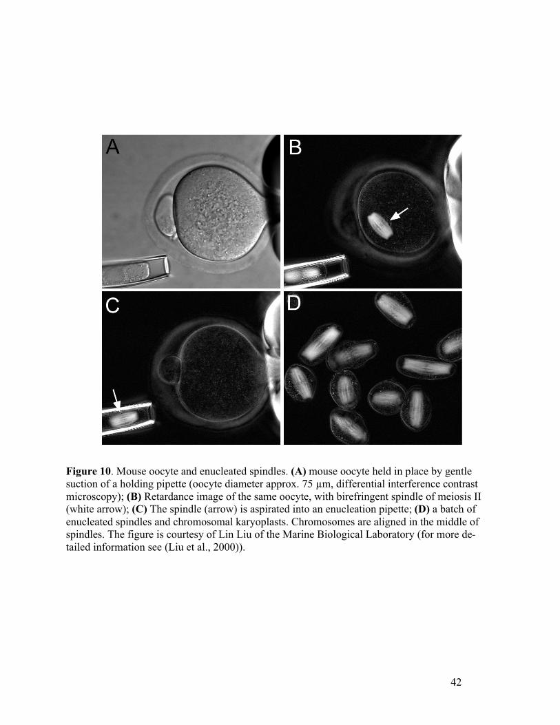
42

Figure 10. Mouse oocyte and enucleated spindles. (A) mouse oocyte held in place by gentlesuction of a holding pipette (oocyte diameter approx. 75 µm, differential interference contrastmicroscopy); (B) Retardance image of the same oocyte, with birefringent spindle of meiosis II(white arrow); (C) The spindle (arrow) is aspirated into an enucleation pipette; (D) a batch ofenucleated spindles and chromosomal karyoplasts. Chromosomes are aligned in the middle ofspindles. The figure is courtesy of Lin Liu of the Marine Biological Laboratory (for more de-tailed information see (Liu et al., 2000)).