Polarization fields and wavefronts of two sheets for ... · PDF filePolarization fields and...

Polarization fields and wavefronts oftwo sheets for understandingpolarization aberrations in opticalimaging systems

José Sasián

Downloaded From: https://www.spiedigitallibrary.org/journals/Optical-Engineering on 4/26/2018 Terms of Use: https://www.spiedigitallibrary.org/terms-of-use

Polarization fields and wavefronts of two sheetsfor understanding polarization aberrations in opticalimaging systems

José Sasián*University of Arizona, College of Optical Sciences, 1630 East University Boulevard, Tucson, Arizona 85721-0094

Abstract. Polarization aberrations by highlighting the concepts of polarization aberration fields and of wave-fronts of two sheets are explained. The fields have a vector character and are derived from the aberration func-tion of plane symmetric systems. It is shown that in the presence of retardance, an incoming optical field is splitinto two fields and therefore one can speak of wavefronts of two sheets. Both concepts, polarization aberrationfields and wavefronts of two sheets, ease the understanding of polarization aberrations. © The Authors. Published bySPIE under a Creative Commons Attribution 3.0 Unported License. Distribution or reproduction of this work in whole or in part requires full attribution ofthe original publication, including its DOI. [DOI: 10.1117/1.OE.53.3.035102]

Keywords: polarization aberrations; optical fields; wavefront of two sheets; optical imaging systems.

Paper 131597P received Oct. 18, 2013; revised manuscript received Jan. 17, 2014; accepted for publication Jan. 22, 2014; publishedonline Mar. 17, 2014.

1 IntroductionThe optical field originated from a point object changes as itinteracts with an optical imaging system. The phase, ampli-tude, and polarization state of the optical field at the entrancepupil of the system can be adversely changed, that is aber-rated, when it arrives at the exit pupil. The polarizationeffects of diattenuation and retardance are one reason forthe optical field to change in an adverse manner for produc-ing optimum imaging. Diattenuation refers to the differencein amplitude that the two polarization states may acquireupon refraction or reflection and retardance to the changein phase that those states can also acquire. Polarization issuesin optical systems have been long known and some effectsand their correction have been reported in the literature.1–8

The subject of polarization aberrations has been defined andstudied previously9,10 using a system’s Jones matrix, whichdepends on the field of view and the aperture of the system.This matrix is expanded, for example, in terms of the Paulispin matrices to provide different terms that represent polari-zation aberrations.

This article provides an alternative way for understandingpolarization aberrations by constructing a set of polarizationfields.11 These basic fields are useful not only for describingthe optical field at the entrance pupil of the optical system butnotably for describing the optical fields at the exit pupil as asuperposition of basic fields. In this article, we provide equa-tions and graphical displays for the first 63 polarizationfields. We express the optical field at the entrance pupilplane of an axially symmetric optical system as

~E ¼ ~Að~H;~ρÞ exp�i2π

λΦð~H;~ρÞ

�; (1)

where the time dependence has been omitted, ~Að~H;~ρÞ is thefield amplitude in vector form, and Φð~H;~ρÞ represents the

optical phase; these depend on the field ~H and aperture ~ρof the system.

We then show that in the presence of retardance theincoming optical field is split into two mutually orthogonalfields.

The surface of constant optical path is the wavefront andthere exist two separated wavefronts, or a wavefront of twosheets, that produce two distinct images.

We develop and highlight the concepts of polarizationfields and of wavefronts of two sheets for understandingpolarization aberrations and imaging. These concepts easethe understanding of how the optical field propagates in anoptical system and provide useful insight. Although theeffects caused by diattenuation and retardance have beenlong known, there still exists a need for a clear theoreticalfoundation of the subject. This article aims at providingsuch a foundation while providing insight for optical engi-neering applications.

2 Construction of the Optical FieldsThe first step is to define the optical field at the entrancepupil, and for this we construct the field amplitude~Að~H;~ρÞ. Since we wish to construct fields that are smoothin their behavior with respect to the field and aperture ofa system and that have symmetric properties, we use theaberration function of a plane symmetric system.12 We estab-lish the unit vector ~i in the field of view to define the direc-tion of plane of symmetry. Since the aberration function isa scalar, it must depend on the dot products of the fieldvector ~H, the aperture vector ~ρ, and the symmetry vector ~i.This aberration function is written as

Wð~i; ~H;~ρÞ ¼X∞

k;m;n;p;q

W2kþnþp;2mþnþq;n;p;q

ð~H · ~HÞkð~ρ · ~ρÞm

× ð~H · ~ρÞnð~i · ~HÞpð~i · ~ρÞq; (2)*Address all correspondence to: José Sasián, E-mail: [email protected]

Optical Engineering 035102-1 March 2014 • Vol. 53(3)

Optical Engineering 53(3), 035102 (March 2014)


http://dx.doi.org/10.1117/1.OE.53.3.035102

http://dx.doi.org/10.1117/1.OE.53.3.035102

http://dx.doi.org/10.1117/1.OE.53.3.035102

http://dx.doi.org/10.1117/1.OE.53.3.035102

http://dx.doi.org/10.1117/1.OE.53.3.035102

http://dx.doi.org/10.1117/1.OE.53.3.035102

where W2kþnþp;2 mþnþq;n;p;q is the coefficient of a particularaberration form defined by the integers k,m, n, p, and q. Thelower indices in the coefficients indicate the algebraicpowers of H, ρ, cosðϕÞ, cosðχÞ, and cosðχ þ ϕÞ in a givenaberration term. The angle χ is between the vectors~i and ~H,and the angle ϕ is between the vectors ~H and ~ρ, and the angleχ þ ϕ is between the vectors ~i and ~ρ.

The fields, called here the ~Rn fields, must have a vectorcharacter; for constructing them we take the gradient of theaberration function for plane symmetric systems,

~Rn ¼ ~∇ρWð~i; ~H;~ρÞ; (3)

where for simplicity the lower index indicates a field number.We construct a complementary set of fields, called the ~Tnfields, by rotating the ~Rn fields by π∕2.

As shown in Fig. 1, we define the unit vector ~r parallel to~ρ, the unit vector ~t perpendicular to ~r, the unit vector ~h par-allel to ~H, the unit vector ~k perpendicular to ~h, and the unitvector ~j perpendicular to ~i. Vectors ~i and ~j are fixed anddefine the coordinate system. The vector ~H ¼ H~h definesthe field point, and the vector ~ρ ¼ ρ~r defines the pupilpoint through which a given ray passes.

The first 63 ~Rn and ~Tn fields that result from taking thegradient of the aberration function for plane symmetric sys-tems are given in Table 1. Piston terms have zero gradientand do not contribute to the fields. As a function of the sym-metry, field, and aperture vectors, there are three fields of firstorder, fifteen fields of third order, and forty five fields of fifthorder. The ~Rn and ~Tn fields are graphically shown inAppendices A and B, respectively; each field display is num-bered and the functional dependence on the field, aperture,and coordinate vectors is also given next to each field. Byconstruction, the ~Rn and ~Tn fields are orthogonal:

~Rn · ~Tn ¼ 0; (4)

A different route to obtain the ~Tn fields is as follows.13

The components of ~Rn are on the pupil plane. Let theunit vectors ~x, ~y, and ~z define a Cartesian coordinate systemwith ~z parallel to the optical axis. Then, we can express the~Tn fields as

~Tn ¼ curl½Wð~i; ~H;~ρÞ~z� ¼ ~x∂Wð~i; ~H;~ρÞ

∂y− ~y

∂Wð~i; ~H;~ρÞ∂x

:

(5)

Since

~Rn ¼ ~∇Wð~i; ~H;~ρÞ ¼ ~x∂Wð~i; ~H;~ρÞ

∂xþ ~y

∂Wð~i; ~H;~ρÞ∂y

: (6)

We have that ~Rn · ~Tn ¼ 0 as ~Tn results by rotation of ~Rn byπ∕2; this is ~Tn ¼ ~j~Rn.

Furthermore, since the curl of ~Rn is zero then the ~Rn fieldsare irrotational; and since the divergence of ~Tn is zero thenthe ~Tn fields are solenoidal. A given vector field that iscontinuous as well as its derivatives can be resolved intoan irrotational part and a solenoidal part. Thus, the ~Rnand ~Tn are an adequate basis to express the amplitude ~Aof an optical field. For completeness purposes, we havepresented the first 63 ~Rn and ~Tn fields. In practice, however,one would be mostly concerned with the low-order fields;high-order fields represent higher-order amplitude polariza-tion aberrations.

3 Optical Field Changes of Second OrderIn this section, we determine the optical field changes to sec-ond order of approximation as a function of the field andaperture of an optical system. These changes relate to thefield amplitude and to the field phase. Assume an opticalsystem where the stop aperture is located at the center ofcurvature of a spherical surface. Therefore, the entrance andexit pupils coincide with the stop location. At the entrancepupil, we have the optical field ~E

~E ¼ ~Að~H;~ρÞ exp�i2π

λΦð~H;~ρÞ

�; (7)

where ~Að~H;~ρÞ, or simply ~A, is the field amplitude andΦð~H;~ρÞ is the optical phase, which depends on the fieldand aperture of the system.

When light is refracted by the surface the polarizationstate may be changed. For the s polarization state, the surfacemay change the field amplitude by the factor ts and introducea phase change ð2π∕λÞδA2ð~ρ · ~ρÞ. For the p polarizationstate, the surface may change the field amplitude by thefactor tp and introduce a phase change ð2π∕λÞðδþΔδÞA2ð~ρ · ~ρÞ. The coefficients δ and Δδ describe phasechanges or retardance, and the parameter A ¼ ni where iis the first-order marginal ray angle (slope) of incidence onthe surface. According to the Fresnel equations, an uncoatedrefracting surface does not contribute retardance; however, ifthe surface has an optical coating then retardance takes place.Retardance is also introduced from light reflection on ametal. The retardance is usually a fraction of a wavelengthand to be significant it requires large angles of incidence. Inhigh-numerical-aperture, multilens systems, the cumulativeeffects of retardance need to be taken into account. The coef-ficients δ and Δδ can analytically be calculated for simplestructures but they can be obtained from phase changesdata provided by an optical thin films program.

Fig. 1 Relation between unit vectors. Vectors~i and ~j are fixed in ori-entation and define the coordinate system. The vectors~i , ~h, and ~r areperpendicular to ~j , ~k , and ~t , respectively.


Sasián: Polarization fields and wavefronts of two sheets for understanding polarization aberrations. . .


Table 1 ~Rn and ~T n fields.

Aberration term ~Rn field ~Tn field

First group

W 01001ð~i · ~ρÞ R1~i T 1

~j

W 11100ð~H · ~ρÞ R2~H T 2H~k

W 02000ð~ρ · ~ρÞ R3~ρ T 3ρ~t

Second group

W 02002ð~i · ~ρÞ2 R4ð~i · ~ρÞ~i T 4ð~i · ~ρÞ~j

W 11011ð~i · ~HÞð~i · ~ρÞ R5ð~i · ~HÞ~i T 5ð~i · ~HÞ~j

W 03001ð~i · ~ρÞð~ρ · ~ρÞ R6ð~ρ · ~ρÞ~i T 6ð~ρ · ~ρÞ~j

R7ð~i · ~ρÞ~ρ T 7ð~i · ~ρÞρ~t

W 12101ð~i · ~ρÞð~H · ~ρÞ R8ð~H · ~ρÞ~i T 8ð~H · ~ρÞ~j

R9ð~i · ~ρÞ~H T 9ð~i · ~ρÞH~k

W 12010ð~i · ~HÞð~ρ · ~ρÞ R10ð~i · ~HÞ~ρ T 10ð~i · ~HÞρ~t

W 21001ð~i · ~ρÞð~H · ~HÞ R11ð~H · ~HÞ~i T 11ð~H · ~HÞ~j

W 21110ð~i · ~HÞð~H · ~ρÞ R12ð~i · ~HÞ~H T 12ð~i · ~HÞH~k

W 04000ð~ρ · ~ρÞ2 R13ð~ρ · ~ρÞ~ρ T 13ð~ρ · ~ρÞρ~t

W 13100ð~H · ~ρÞð~ρ · ~ρÞ R14ð~H · ~ρÞ~ρ R15ð~ρ · ~ρÞ~H T 14ð~H · ~ρÞρ~t T 15ð~ρ · ~ρÞH~k

W 22200ð~H · ~ρÞ2 R16ð~H · ~ρÞ~H T 16ð~H · ~ρÞH~k

W 22000ð~H · ~HÞð~ρ · ~ρÞ R17ð~H · ~HÞ~ρ T 17ð~H · ~HÞρ~t

W 31100ð~H · ~HÞð~H · ~ρÞ R18ð~H · ~HÞ~H T 18ð~H · ~HÞH~k

Third group

W 03003ð~i · ~ρÞ3 R19ð~i · ~ρÞ2~i T 19ð~i · ~ρÞ2~j

W 12012ð~i · ~HÞð~i · ~ρÞ2 R20ð~i · ~HÞð~i · ~ρÞ~i T 20ð~i · ~HÞð~i · ~ρÞ~j

W 21021ð~i · ~HÞ2ð~i · ~ρÞ R21ð~i · ~HÞ2~i T 21ð~i · ~HÞ2~j

W 04002ð~i · ~ρÞ2ð~ρ · ~ρÞ R22ð~i · ~ρÞð~ρ · ~ρÞ~i R23ð~i · ~ρÞ2~ρ T 22ð~i · ~ρÞð~ρ · ~ρÞ~j T 23ð~i · ~ρÞ2ρ~t

W 13011ð~i · ~HÞð~i · ~ρÞð~ρ · ~ρÞ R24ð~i · ~HÞð~ρ · ~ρÞ~i T 24ð~i · ~HÞð~ρ · ~ρÞ~j

R25ð~i · ~HÞð~i · ~ρÞ~ρ T 25ð~i · ~HÞð~i · ~ρÞρ~t

W 22002ð~i · ~ρÞ2ð~H · ~HÞ R26ð~i · ~ρÞð~H · ~HÞ~i T 26ð~i · ~ρÞð~H · ~HÞ~j

W 22020ð~i · ~HÞ2ð~ρ · ~ρÞ R27ð~i · ~HÞ2~ρ T 27ð~i · ~HÞ2ρ~t

W 31011ð~i · ~HÞð~i · ~ρÞð~H · ~HÞ R28ð~i · ~HÞð~H · ~HÞ~i T 28ð~i · ~HÞð~H · ~HÞ~j

W 13102ð~i · ~ρÞ2ð~H · ~ρÞ R29ð~i · ~ρÞð~H · ~ρÞ~i R30ð~i · ~ρÞ2 ~H T 29ð~i · ~ρÞð~H · ~ρÞ~j T 30ð~i · ~ρÞ2H~k

W 22111ð~i · ~HÞð~i · ~ρÞð~H · ~ρÞ R31ð~i · ~HÞð~H · ~ρÞ~i R32ð~i · ~HÞð~i · ~ρÞ~H T 31ð~i · ~HÞð~H · ~ρÞ~j T 32ð~i · ~HÞð~i · ~ρÞH~k




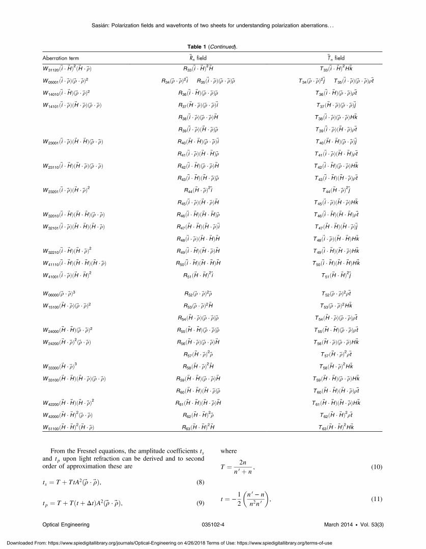
From the Fresnel equations, the amplitude coefficients tsand tp upon light refraction can be derived and to secondorder of approximation these are

ts ¼ T þ TtA2ð~ρ · ~ρÞ; (8)

tp ¼ T þ Tðtþ ΔtÞA2ð~ρ · ~ρÞ; (9)

where

T ¼ 2nn 0 þ n

; (10)

t ¼ −1

2

�n 0 − nn2n 0

�; (11)

Table 1 (Continued).

Aberration term ~Rn field ~Tn field

W 31120ð~i · ~HÞ2ð~H · ~ρÞ R33ð~i · ~HÞ2 ~H T 33ð~i · ~HÞ2H~k

W 05001ð~i · ~ρÞð~ρ · ~ρÞ2 R34ð~ρ · ~ρÞ2~i R35ð~i · ~ρÞð~ρ · ~ρÞ~ρ T 34ð~ρ · ~ρÞ2~j T 35ð~i · ~ρÞð~ρ · ~ρÞρ~t

W 14010ð~i · ~HÞð~ρ · ~ρÞ2 R36ð~i · ~HÞð~ρ · ~ρÞ~ρ T 36ð~i · ~HÞð~ρ · ~ρÞρ~t

W 14101ð~i · ~ρÞð~H · ~ρÞð~ρ · ~ρÞ R37ð~H · ~ρÞð~ρ · ~ρÞ~i T 37ð~H · ~ρÞð~ρ · ~ρÞ~j

R38ð~i · ~ρÞð~ρ · ~ρÞ~H T 38ð~i · ~ρÞð~ρ · ~ρÞH~k

R39ð~i · ~ρÞð~H · ~ρÞ~ρ T 39ð~i · ~ρÞð~H · ~ρÞρ~t

W 23001ð~i · ~ρÞð~H · ~HÞð~ρ · ~ρÞ R40ð~H · ~HÞð~ρ · ~ρÞ~i T 40ð~H · ~HÞð~ρ · ~ρÞ~j

R41ð~i · ~ρÞð~H · ~HÞ~ρ T 41ð~i · ~ρÞð~H · ~HÞρ~t

W 23110ð~i · ~HÞð~H · ~ρÞð~ρ · ~ρÞ R42ð~i · ~HÞð~ρ · ~ρÞ~H T 42ð~i · ~HÞð~ρ · ~ρÞH~k

R43ð~i · ~HÞð~H · ~ρÞ~ρ T 43ð~i · ~HÞð~H · ~ρÞρ~t

W 23201ð~i · ~ρÞð~H · ~ρÞ2 R44ð~H · ~ρÞ2~i T 44ð~H · ~ρÞ2~j

R45ð~i · ~ρÞð~H · ~ρÞ~H T 45ð~i · ~ρÞð~H · ~ρÞH~k

W 32010ð~i · ~HÞð~H · ~HÞð~ρ · ~ρÞ R46ð~i · ~HÞð~H · ~HÞ~ρ T 46ð~i · ~HÞð~H · ~HÞρ~t

W 32101ð~i · ~ρÞð~H · ~HÞð~H · ~ρÞ R47ð~H · ~HÞð~H · ~ρÞ~i T 47ð~H · ~HÞð~H · ~ρÞ~j

R48ð~i · ~ρÞð~H · ~HÞ~H T 48ð~i · ~ρÞð~H · ~HÞH~k

W 32210ð~i · ~HÞð~H · ~ρÞ2 R49ð~i · ~HÞð~H · ~ρÞ~H T 49ð~i · ~HÞð~H · ~ρÞH~k

W 41110ð~i · ~HÞð~H · ~HÞð~H · ~ρÞ R50ð~i · ~HÞð~H · ~HÞ~H T 50ð~i · ~HÞð~H · ~HÞH~k

W 41001ð~i · ~ρÞð~H · ~HÞ2 R51ð~H · ~HÞ2~i T 51ð~H · ~HÞ2~j

W 06000ð~ρ · ~ρÞ3 R52ð~ρ · ~ρÞ2~ρ T 52ð~ρ · ~ρÞ2ρ~t

W 15100ð~H · ~ρÞð~ρ · ~ρÞ2 R53ð~ρ · ~ρÞ2 ~H T 53ð~ρ · ~ρÞ2H~k

R54ð~H · ~ρÞð~ρ · ~ρÞ~ρ T 54ð~H · ~ρÞð~ρ · ~ρÞρ~t

W 24000ð~H · ~HÞð~ρ · ~ρÞ2 R55ð~H · ~HÞð~ρ · ~ρÞ~ρ T 55ð~H · ~HÞð~ρ · ~ρÞρ~t

W 24200ð~H · ~ρÞ2ð~ρ · ~ρÞ R56ð~H · ~ρÞð~ρ · ~ρÞ~H T 56ð~H · ~ρÞð~ρ · ~ρÞH~k

R57ð~H · ~ρÞ2~ρ T 57ð~H · ~ρÞ2ρ~t

W 33300ð~H · ~ρÞ3 R58ð~H · ~ρÞ2 ~H T 58ð~H · ~ρÞ2H~k

W 33100ð~H · ~HÞð~H · ~ρÞð~ρ · ~ρÞ R59ð~H · ~HÞð~ρ · ~ρÞ~H T 59ð~H · ~HÞð~ρ · ~ρÞH~k

R60ð~H · ~HÞð~H · ~ρÞ~ρ T 60ð~H · ~HÞð~H · ~ρÞρ~t

W 42200ð~H · ~HÞð~H · ~ρÞ2 R61ð~H · ~HÞð~H · ~ρÞ~H T 61ð~H · ~HÞð~H · ~ρÞH~k

W 42000ð~H · ~HÞ2ð~ρ · ~ρÞ R62ð~H · ~HÞ2~ρ T 62ð~H · ~HÞ2ρ~t

W 51100ð~H · ~HÞ2ð~H · ~ρÞ R63ð~H · ~HÞ2 ~H T 63ð~H · ~HÞ2H~k




Δt ¼ 1

2

�n 0 − nnn 0

�2

: (12)

The optical field is described at the entrance pupil planelocated at the surface’s center of curvature, and to secondorder of approximation, the unit vector ~r is in the planeof incidence of a ray specified by ~H and ~ρ, and the unit vector~t is perpendicular to the plane of incidence of the ray.

After light refraction the field ~E 0 at the exit pupil can bewritten as if both amplitude and phase changes occur simul-taneously

~E 0 ¼ exp

�i2π

λδA2ð~ρ · ~ρÞ

��tsð~E ·~tÞ~tþ exp

�i2π

λΔδA2ð~ρ · ~ρÞ

�

× tpð~E · ~rÞ~r�; (13)

or as if amplitude and phase changes occur sequentially.For simplicity, we take the later route.

When there is no retardance Δδ ¼ 0 between thetwo polarization states, the optical field ~E 0 can be writtenas

~E 0 ¼ exp

�i2π


�½tsð~E · ~tÞ~tþ tpð~E · ~rÞ~r�

¼ exp

�i2π


�f½T þ TtA2ð~ρ · ~ρÞ�ð~E ·~tÞ~t

þ ½T þ Tðtþ ΔtÞA2ð~ρ · ~ρÞ�ð~E · ~rÞ~rg

¼ exp

�i2π


�½T~Eþ TtA2ð~ρ · ~ρÞ~E

þ TΔtA2ð~E · ~ρÞ~ρ�: (14)

When the retardance Δδ is introduced the optical field ~E�

becomes

~E� ¼ exp

�i2π

λ

�1

2ΔδA2ð~ρ · ~ρÞ

��

×

(ð~E 0 · ~tÞ~t exp�−i 2πλ 1

2ΔδA2ð~ρ · ~ρÞ�þ

ð~E 0 · ~rÞ~r exp�i 2πλ

12ΔδA2ð~ρ · ~ρÞ�

): (15)

We define the unit vector ~a parallel to ~E 0 and the unit vec-tor ~b perpendicular to ~E 0. Then, we write ~E 0 ¼ j~E 0j~a anddefine a field ~E 0⊥ ¼ j~E 0j~b perpendicular to the field ~E 0.

The unit vectors ~r and ~t can be decomposed in a compo-nent parallel to ~a and a component parallel to ~b, where wehave j~aj ¼ 1, j~bj ¼ 1, and ~a · ~b ¼ 0. The decomposition is

~r ¼ ð~a · ~rÞ~aþ ð~b · ~rÞ~b ~t ¼ ð~a ·~tÞ~aþ ð~b ·~tÞ~b: (16)

We also can write the relationships

ð~E 0 · ~rÞ~r ¼ ð~a · ~rÞ2~E 0 þ ð~a · ~rÞð~b · ~rÞ~E 0⊥

ð~E 0 ·~tÞ~t ¼ ð~a · ~tÞ2~E 0 þ ð~a · ~tÞð~b ·~tÞ~E 0⊥: (17)

The optical field at the exit pupil then becomes

~E� ¼ exp

�i2π

λ

�1


��

×

8<:½ð~a ·~tÞ2~E 0 þ ð~a ·~tÞð~b ·~tÞ~E 0⊥� exp

h−i 2πλ


iþ

½ð~a · ~rÞ2~E 0 þ ð~a · ~rÞð~b · ~rÞ~E 0⊥� exphi 2πλ


i9=;:

(18)

The field ~E� can be separated into a component ~Eo

parallel and a component ~Ee perpendicular to the field ~E 0.These field components ~Eo and ~Ee can be written (seeAppendix C) as

~Eo ¼ ~E 0exp

�i2π

λ

�1


�� ffiffiffiffiffiffiffiffiffiffiffiffiffiffiffiffiffiffiffiffiffiffiffiffiffiffiffiffiffiffiffiffiffiffiffiffiffiffiffiffiffiffiffiffiffiffiffiffiffiffiffiffiffiffiffiffiffiffiffiffiffiffiffiffiffiffiffiffiffiffiffiffiffiffiffiffiffiffiffiffiffiffiffiffiffiffiffiffiffiffiffiffiffiffiffiffiffiffiffiffiffiffiffiffiffiffiffiffiffiffiffiffiffiffiffiffiffiffiffiffiffiffiffiffiffiffiffiffiffiffiffiffiffiffiffiffiffiffiffiffiffiffiffiffiffiffiffiffiffiffiffiffi�cos2

�2π

λ

1

2½ΔδA2ð~ρ · ~ρÞ

��þ sin2

�2π

λ

1

2½ΔδA2ð~ρ · ~ρÞ�

�½ð~a · ~rÞ2 − ð~a ·~tÞ2�2

�s

× exp

�i × arct

�Tan

�2π

λ

1


�½ð~a · ~rÞ2 − ð~a ·~tÞ2�

��≅ ~E 0

exp

�i2π

λ

�ΔδA2ð~a · ~ρÞ2

��(19)

and

~Ee ¼ ~E 0⊥exp

�i2π

λ

�1


�þ i

π

2

�

×�2ð~a · ~rÞð~b · ~rÞ

��sin

2π

λ

1


�

≅ ~E 0⊥exp

�i2π

λ

�1


�þ i

π

2

�

×�2π

λΔδA2ð~a · ~ρÞð~b · ~ρÞ

�: (20)

We note that j~Eoj2 þ j~Eej2 ¼ j~E 0j2 and thus the energy inthe ~E 0 field is conserved and shared by the ~Eo and ~Ee fields.

The superscripts o and e are used to avoid confusion withthe usage of parallel and perpendicular as they often refer tothe plane of light incidence.

In this decomposition, each field component, ~Eo and ~Ee,has amplitude and phase and is perpendicular to the otherover the entire pupil. Thus, the incoming optical field issplit into two fields. Furthermore, for a given optical pathlength OPL from an object point, a wavefront can be definedfor the ~Eo field. Similarly, for the same OPL a distinct andseparated wavefront can be defined for the ~Ee field.Therefore, in the presence of retardance, we can speak ofthe concept of a wavefront of two sheets, one sheet belong-ing to the ~Eo field component, the other sheet belonging tothe ~Ee field component. Given the wavefront of two sheets




then two distinct images of the source point can be expected.Retardance, and therefore wavefront splitting, can be intro-duced by a thin film coating on a lens, by reflection on metal,or by a birefringent material. For example, by placing a z-cut,uniaxial crystal in an optical system with its optical axisaligned with the system’s optical axis, one can introduceretardance due to the crystal birefringence.

4 Optical Field upon Stop ShiftingNow, we consider the optical field when the aperture stop isnot located at the center of curvature of the spherical surface.

For this we perform stop shifting, which is achieved byreplacing in the fields ~Eo and ~Ee the aperture vector ~ρ

with the shift vector ~ρshift ¼ ~ρþ ðA∕AÞ~H and by term expan-sion.11 The factor A ¼ ni where i is the first-order chief rayangle of incidence on the surface, and the factor A ¼ niwhere i is the first-order marginal angle of incidence. Weonly retain second-order terms as a function of the field vec-

tor ~H and the aperture vector ~ρ.By substitution of the shift vector ~ρshift in ~Eo the field is

obtained for a general stop location

~Eoð~H;~ρÞ ¼ T exp

�i2π

λδ½A2ð~ρ · ~ρÞ þ 2AAð~H · ~ρÞ þ A2ð~H · ~HÞ�

�

×

~Eþ t½A2ð~ρ · ~ρÞ þ 2AAð~H · ~ρÞ þ A2ð~H · ~HÞ�~EþΔtf½A2ð~E · ~ρÞ~ρþ AAð~E · ~HÞ~ρ� þ ½AAð~E · ~ρÞ~H þ A2ð~E · ~HÞ~H�g

!

× exp

�i2π

λfΔδ½A2ð~a · ~ρÞ2 þ 2AAð~a · ~ρÞð~a · ~HÞ þ A2ð~a · ~HÞ2�g

�: (21)

Similarly, for the ~Ee field component after neglectingfourth-order terms we can write

~Eeð ~H;~ρÞ¼T exp

�i2π

λ

��δþ1

2Δδ��

A2ð~ρ ·~ρÞ

þ2AAð ~H ·~ρÞþA2ð ~H · ~HÞþλ

4

��

× ~E⊥�2π

λΔδ�Að~a ·~ρÞð~b ·~ρÞþAAð~a · ~HÞð~b ·~ρÞþAAð~a ·~ρÞð~b · ~HÞþA2ð~a · ~HÞð~b · ~HÞ

��;

(22)

where ~E⊥ is the optical field ~E rotated 90 deg. In both ofthese expressions, the field ~E is at the entrance pupil afterstop shifting. The field ~E is either already known or isobtained by substitution of the shift ~ρshift vector in thefield at the plane of the surface center of curvature.

5 Polarization Aberration CoefficientsWe now determine the coefficients that define the opticalfield for an optical system of several surfaces. We assumethat to second order the individual surface coefficients addto form the coefficients for the entire optical system. Thetransmission from two surfaces is the product of the individ-ual surface transmissions. However, when the amplitudefactors have zero- and second-order terms, the second-orderterms of the product are the sums of the second-order termsof the factors (weighted by the zero-order terms). Regardingphase, it follows from the fact that optical paths add,that we can add second-order phase terms. However, weneglect some extrinsic14 second-order terms that might bepresent due to the interaction between second-order termsdue to light refraction and second-order terms due to polari-zation retardance. These extrinsic terms depend on theproduct of the gradient of second-order aberrations. Sincesecond-order effects from retardance are small then theextrinsic contributions are expected to be comparatively neg-ligible. Effectively, phase contributions due to pure refraction

or reflection are accurately accounted by the first-order raytrace. However, when the phase is changed due to polariza-tion retardance, then the standard first-order ray trace basedon the surface optical powers will not fully account for first-order ray paths. There will be a small error which would beaccounted for with extrinsic terms. One way to avoid first-order errors is to include the second-order phase contributions,optical power, from retardance in the first-order ray trace.

Table 2 presents a summary of second-order polarizationaberration coefficients for a system of q surfaces. These coef-ficients are the sums of individual surface coefficients foramplitude and phase terms. Their calculation requires theray tracing of a marginal and a chief first-order (paraxial)rays. The factor A ¼ ni is the first-order chief ray refractioninvariant, and the factor A ¼ ni is the first-order marginal rayrefraction invariant. Those rays have paraxial angles (slopes)of incidence i and i at a given system surface. Coefficientssimilar to the presented in Table 2 have been previouslyintroduced by Chipman.15

To express the optical field at the exit pupil, we alsodefine the retardance functions δð~H;~ρÞ, Δδað~H;~ρÞ,Δδbð~H;~ρÞ, Δδcð~H;~ρÞ as

δð~H;~ρÞ ¼ δ1ð~ρ · ~ρÞ þ δ2ð~H · ~ρÞ þ δ3ð~H · ~HÞ (23)

Δδað~H;~ρÞ ¼ Δδ1ð~ρ · ~ρÞ þ Δδ2ð~H · ~ρÞ þ Δδ3ð~H · ~HÞ (24)

Δδbð~H;~ρÞ ¼ Δδ1ð~a · ~ρÞ2 þΔδ2ð~a · ~HÞð~a · ~ρÞ þΔδ3ð~a · ~HÞ2

(25)

Δδcð~H;~ρÞ ¼ Δδ1ð~a · ~ρÞð~b · ~ρÞ þ Δδ2ð~a · ~ρÞð~b · ~HÞ þ Δδ2

× ð~a · ~HÞð~b · ~ρÞ þ Δδ3ð~a · ~HÞð~b · ~HÞ: (26)




6 Optical Field at the Exit PupilIn this section, we present expressions for the optical field atthe exit pupil to second order of approximation. In theabsence of retardance Δδ ¼ 0 and using the polarizationaberration coefficients in Table 2, we can write the opticalfield ~Eo at the exit pupil of an optical system as

~Eo ¼ ~A 0ð~H;~ρÞ exp�i2π

λ½Φð~H;~ρÞ þ δð~H;~ρÞ�

�; (27)

where the amplitude function ~A 0ð~H;~ρÞ is

~A 0ð~H;~ρÞ

¼�Tq

~Aþ P1ð~ρ · ~ρÞ~Aþ P2ð~H · ~ρÞ~Aþ P3ð~H · ~HÞ~AP4ð~A · ~ρÞ~ρþ P5½ð~A · ~HÞ~ρþ ð~A · ~ρÞ~H� þ P6ð~A · ~HÞ~H

�;

(28)

and the retardance function δð~H;~ρÞ is

δð~H;~ρÞ ¼ δ1ð~ρ · ~ρÞ þ δ2ð~H · ~ρÞ þ δ3ð~H · ~HÞ: (29)

The terms in the amplitude function ~A 0ð~H;~ρÞ representchanges to the field amplitude and orientation. The fieldamplitude ~A 0ð~H;~ρÞ at the exit pupil depends on the fieldamplitude ~A ¼ ~Að~H;~ρÞ at the entrance pupil. If we have auniform field amplitude ~A ¼~i, a linearly polarized field,then the field amplitude ~A 0ð~H;~ρÞ involves the ~Rn fields~R6 through ~R12. These seven ~Rn fields are often the ampli-tude changes that take place and are shown in Fig. 2. If wehave a radial field amplitude ~A ¼ ~r, then the field amplitude~A 0ð~H;~ρÞ involves the ~Rn fields ~R13 through ~R18, which areshown in Fig. 3.

The terms in retardance function δð~H;~ρÞ represent changeof focus, change of magnification, and piston aberrations.Therefore, in the presence of retardance δ ≠ 0, the first-order properties of the system change.

In the absence of retardance, Δδ ¼ 0, the ~Ee field com-ponent is absent too.

When there is retardance, Δδ ≠ 0, the ~Eo field componentcan be written as

~Eo ¼ ~A 0ð~H;~ρÞ exp�i2π

λ½Φð~H;~ρÞ þ δð~H;~ρÞ þΔδbð~H;~ρÞ�

�:

(30)

In this case, the field phase includes three more termsaccording to the retardance function

Δδbð~H;~ρÞ ¼ Δδ1ð~a · ~ρÞ2 þΔδ2ð~a · ~HÞð~a · ~ρÞ þΔδ3ð~a · ~HÞ2:(31)

When ~a ¼ ~i these terms are astigmatism, anamorphicmagnification, and piston aberrations.

Furthermore, when there is retardance, Δδ ≠ 0, the ~Ee

field component can be written as

~Eeð~H;~ρÞ ¼ ~A0⊥ð~H;~ρÞ�2π

λΔδcð~H;~ρÞ

�

× exp

�i2π

λ

�Φð~H;~ρÞ þ δð~H;~ρÞ þ 1

2Δδað~H;~ρÞ þ λ

4

��;

(32)

where ~A 0⊥ð~H;~ρÞ ¼ j~A 0ð~H;~ρÞj~b. In this case, the ~Ee fieldamplitude is strongly apodized by the function

Δδcð~H;~ρÞ ¼ Δδ1ð~a · ~ρÞð~b · ~ρÞ þ Δδ2ð~a · ~ρÞð~b · ~HÞ þ Δδ2

× ð~a · ~HÞð~b · ~ρÞ þ Δδ3ð~a · ~HÞð~b · ~HÞ: (33)

The phase for the ~Ee field includes three more termsthrough the retardance function

Δδað~H;~ρÞ ¼ Δδ1ð~ρ · ~ρÞ þ Δδ2ð~H · ~ρÞ þ Δδ3ð~H · ~HÞ:(34)

These terms change the first-order properties of the sys-tem and represent change of focus, change of magnification,and piston aberrations.

7 Pupil and Image Plane IrradiancesIn this section, we illustrate irradiance and the point spreadfunction for the ~Eo and ~Ee fields when ~a ¼ ~i and ~H ¼ 0. Therows in Fig. 4 shows three cases for different amounts ofretardance Δδ ¼ λ∕8, Δδ ¼ λ∕4, and Δδ ¼ λ∕2. For thefield ~Eo, column A gives the irradiance at the exit pupiland column B gives the point spread function assumingno phase errors and that the astigmatism term Δδ1ð~a · ~ρÞ2has been corrected. For the field ~Ee, column C gives the irra-diance and column D gives the point spread function assum-ing no phase errors. Column E gives the incoherent sum ofcolumns B and D.

Note that the irradiance distribution for the ~Eo field at theexit pupil is reminiscent of the irradiance distribution undercrossed polarizers of a lens that contributes diattenuation.However, in the former case, the pattern resembling a crossappears illuminated (see case A for Δδ ¼ λ∕2) and in thelatter case the pattern appears dark.

A more realistic case is when the astigmatism termΔδbð~H;~ρÞ ¼ Δδ1ð~a · ~ρÞ2 is present. Then, the irradiancepatterns as calculated at the medial focus change as shownin Fig. 5. Note that for a retardance Δδ ¼ λ∕4, there is

Table 2 Polarization aberration coefficients for a system of qsurfaces.

P1 ¼ TqPq

j¼1 ðtA2Þj δ1 ¼Pqj¼1 ðδA2Þj

P2 ¼ 2TqPq

j¼1 ðtAAÞj δ2 ¼ 2Pq

j¼1 ðδAAÞjP3 ¼ Tq

Pqj¼1 ðt A2Þj δ3 ¼Pq

j¼1 ðδA2ÞjP4 ¼ Tq

Pqj¼1 ðΔtA2Þj Δδ1 ¼Pq

j¼1 ðΔδA2ÞjP5 ¼ Tq

Pqj¼1 ðΔtAAÞj Δδ2 ¼Pq

j¼1 ðΔδAAÞjP6 ¼ Tq

Pqj¼1 ðΔt A2Þj Δδ3 ¼Pq

j¼1 ðΔδA2Þjt j ¼ − 1

2 ðn0−n

n2n 0 Þj Δt j ¼ 12 ðn

0−nnn 0 Þ2j

T j ¼Qj

k¼1 ð 2nnþn 0Þk A ¼ ni

A ¼ ni




a significant change in the point spread function as calculatedat medial focus.

8 Elliptical PolarizaitonIn the presence of retardance, the state of polarization ofa linearly polarized field changes to elliptical polarization.It is also of interest to determine the properties of the polari-zation ellipse.

Using the definitions,

tanðαÞ ¼ j~Eejj~Eoj

; (35)

tanðχÞ ¼ ∓ba: (36)

We write the relationships for the orientation and ellipticityof the polarization ellipse,

tanð2ψÞ ¼ tanð2αÞ cos�2π

λΔδd

�; (37)

sinð2χÞ ¼ sinð2αÞ sin�2π

λΔδd

�; (38)

where ψ is the angle that the major axis of the polarizationellipse makes with the ~a direction, and the ellipticity tanðχÞ isthe ratio of the minor b to major axis a of the polarizationellipse.

We can approximate the tangent of α to second order by

tanðαÞ ¼ j~Eejj~Eoj

≅2π

λΔδc: (39)

The retardance Δδd is given by

Δδd ¼ Δδbð~H;~ρÞ − 1

2Δδað~H · ~ρÞ − λ

4: (40)

Then, we can write

cos

�2π

λΔδd

�¼ sin

�2π

λ

�Δδbð~H;~ρÞ − 1

2Δδað~H · ~ρÞ

��

≅2π

λ

�Δδbð~H;~ρÞ − 1

2Δδað~H · ~ρÞ

�;

(41)

which is a second-order quantity. Similarly, the parameter αto second order is given by

α ≅2π

λΔδcð~H;~ρÞ

¼ 2π

λ

�Δδ1ð~a · ~ρÞð~b · ~ρÞ þ Δδ2ð~a · ~ρÞð~b · ~HÞþΔδ2ð~a · ~HÞð~b · ~ρÞ þ Δδ3ð~a · ~HÞð~b · ~HÞ

�: (42)

Therefore, the angle ψ is a fourth-order quantity implyingthat for a small amount of retardance Δδ the orientation of

Fig. 2 Graphical display of the ~R6 to ~R12 fields.





the polarization ellipse is not too different from the orienta-tion of the field amplitude ~A 0ð~H;~ρÞ.

For sin½ð2π∕λÞΔδd�, we can write to second order ofapproximation

sin

�2π

λΔδd

�≅ 1: (43)

Then, the ellipticity for small amounts of retardance Δδcan be approximated to second order by

tanðχÞ ¼ ba

≅2π

λ

�Δδ1ð~a · ~ρÞð~b · ~ρÞ þ Δδ2ð~a · ~ρÞð~b · ~HÞþΔδ2ð~a · ~HÞð~b · ~ρÞ þ Δδ3ð~a · ~HÞð~b · ~HÞ

�:

(44)

For the zero field position ~H ¼ 0, the ellipticity is maxi-mum when the aperture vector ~ρ is at an angle of 45 deg withrespect to the vector ~a, and at the edge of the aperturej~ρj ¼ 1. In this case, we can write

ba≅π

λΔδ1: (45)

For the case of having Δδ1 ¼ λ∕10, the ellipticity is esti-mated to be 0.314. Figure 6 left shows a polarization pupilmap for a refractive system with no coatings and therefore noretardance Δδ1 ¼ 0. However, when the lens surfaces arecoated, retardance is introduced and the polarizationstate changes to elliptical as shown with ellipses in Fig. 6right.

9 SummaryA useful way to understand polarization aberrations is by theconcepts of polarization fields and of wavefronts of twosheets. In this article, we have constructed polarization fieldsrequiring smoothness, symmetry properties, and physicalplausibility. To this end, we have used the aberration function

of a plane symmetrical system and have taken the gradient topass from a scalar field to a vector field. We have thusdefined the ~Rn and ~Tn fields as an adequate basis to describepolarization fields. These fields carry both aperture and fielddependence. For completeness purposes, we have presentedthe first 63 ~Rn and ~Tn fields. However, given an axially sym-metric system and a linear input polarization state, one wouldbe mostly concerned with the seven third-order ~Rn fields (~R6

to ~R12). If the input polarization state is radial, then onewould be mostly concerned with the six third-order ~Rn fields(~R13 to ~R18). Higher-order fields represent higher-orderamplitude polarization aberrations.

For an axially symmetric system, we have expressed tosecond order the optical field at the exit pupil as a superpo-sition of polarization field components. We also have pro-vided the coefficients of these fields as a function of thesystem parameters and have used sums over the system sur-faces to find the polarization aberration coefficients for theentire system. Data from a first-order marginal and chief rayis used to compute the polarization aberration coefficients.

In the absence of retardance Δδ ¼ 0 introduced by anoptical surface, the field amplitude changes its orientationand magnitude. In addition, the first-order properties ofthe system change as the optical phase changes accordingto the function δð~H;~ρÞ, which represents change of focus,change of magnification, and piston aberrations.

In the presence of retardance Δδ ≠ 0, the incoming opti-cal field is split into two field components ~Eo and ~Ee. Each ofthese components is perpendicular to the other, and fora given optical path length, a wavefront of two sheets isdefined. In addition, the phenomenon of elliptical polariza-tion takes place. For small amounts of retardance, the orien-tation of the polarization ellipse is a fourth-order quantityand substantially coincides with the orientation of thetransmitted field amplitude. The ellipticity is however asecond-order quantity and is proportional to the amount ofretardance.

The treatment presented in this article is based onprevious work, and it is a refinement in that it provides ana-lytically and graphically up to the first 63 ~Rn and ~Tn fields.

Fig. 4 Three cases of retardance, Δδ ¼ λ∕8, Δδ ¼ λ∕4, and Δδ ¼ λ∕2. For the field ~Eocolumn A gives

the irradiance at the exit pupil and column B gives the point spread function assuming no phase errors.For the field ~Ee column C gives the irradiance and column D gives the point spread function assuming nophase errors. Column E gives the incoherent sum of columns B and D.




Most importantly, this article highlights the occurrence ofa wavefront of two sheets. In the treatment presentedhere. the phase calculation avoids a linear approximation tothe exponential function and shows that the optical field issplit into two mutually orthogonal components that wouldproduce two distinct images. We also illustrate the amplitudeapodization for the two mutually perpendicular fields and thepoint spread function due to both fields. Effectively, in thepresence of retardance, an incoming beam is split into twobeams and therefore accounting for the effects from eachbeam is of relevance.

The understanding of the classic aberrations of spherical,coma, astigmatism, field curvature, and distortion oftenpresents difficulties. The case of understanding polarizationaberrations can be more challenging. However, with the con-cepts of polarization fields and wavefront of two sheets,

the understanding of polarization aberrations is eased, andsimplicity and useful insights are gained. This articleaims at providing a theoretical foundation to ease the under-standing of polarization aberrations for optical engineeringapplications.

Appendix AFigure 7 shows a graphical display of the ~R1 to ~R63

fields.

Appendix BFigure 8 shows a graphical display of the ~T1 to ~T63

fields.

Fig. 5 Three cases of retardance,Δδ ¼ λ∕8,Δδ ¼ λ∕4, andΔδ ¼ λ∕2. For the field ~Eocolumn A gives the

irradiance at the exit pupil and column B gives the point spread function calculated at medial focus. Forthe field ~E

ecolumn C gives the irradiance and column D gives the point spread function calculated at

medial focus. Column E gives the incoherent sum of columns B and D.

Fig. 6 (a) Polarization pupil map showing the orientation and magnitude of the field at the exit pupil of alens system. At the entrance pupil the field is uniform and linearly polarized. (b) When coatings are addedto the surfaces retardance is introduced and the polarization state changes from linear to elliptical asshown by ellipses.




Fig. 8 Graphical display of the ~T 1 to ~T 63 fields.




Appendix CThis appendix provides some algebraic steps in obtaining the optical field. We start with the expression for the ~E� field

~E� ¼ exp

�i2π

λ

�1


��8><>:

½ð~a ·~tÞ2~E 0 þ ð~a ·~tÞð~b ·~tÞ~E 0⊥� exph−i 2πλ


iþ

½ð~a · ~rÞ2~E 0 þ ð~a · ~rÞð~b · ~rÞ~E 0⊥iexphi 2πλ


i9>=>;: (46)

The field ~Eo is

~Eo ¼ exp

�i2π

λ

�δA2ð~ρ · ~ρÞ þ 1


��~E 0

8<:

ð~a ·~tÞ2 exph−i 2πλ


iþ

ð~a · ~rÞ2 exphi 2πλ


i9=;: (47)

By expressing the exponential function with a cosine and a sine term, we can write

~E0 ¼ exp

�i2π

λ



��264 ½ð~a ·~tÞ2~E 0�cosn− 2π

λ12½ΔδA2ð~ρ · ~ρÞ�

o− i sin

n2πλ


o�þ

½ð~a · ~rÞ2~E 0�cosn2πλ


oþ i sin

n2πλ


o�375:

(48)

Or,

~E0 ¼ exp

�i2π

λ½δA2ð~ρ · ~ρÞ þ 1


�~E 0�cos

�2π

λ

1


�þ i sin

�2π

λ

1


�½ð~a · ~rÞ2 − ð~a ·~tÞ2�

�:

(49)

By expressing the complex factor in terms of its argument and phase, we can write

~E0¼ ~E 0exp

�i2π

λ

�δA2ð~ρ ·~ρÞþ1

2ΔδA2ð~ρ ·~ρÞ

�� ffiffiffiffiffiffiffiffiffiffiffiffiffiffiffiffiffiffiffiffiffiffiffiffiffiffiffiffiffiffiffiffiffiffiffiffiffiffiffiffiffiffiffiffiffiffiffiffiffiffiffiffiffiffiffiffiffiffiffiffiffiffiffiffiffiffiffiffiffiffiffiffiffiffiffiffiffiffiffiffiffiffiffiffiffiffiffiffiffiffiffiffiffiffiffiffiffiffiffiffiffiffiffiffiffiffiffiffiffiffiffiffiffiffiffiffiffiffiffiffiffiffiffiffiffiffiffiffiffiffiffiffiffiffiffiffiffiffiffiffiffiffi�cos2

�2π

λ

1

2½ΔδA2ð~ρ ·~ρÞ�

�þsin2

�2π

λ

1


�½ð~a ·~rÞ2−ð~a ·~tÞ2�2

�s

×exp�i×arct

�Tan

�2π

λ

1


�½ð~a ·~rÞ2−ð~a ·~tÞ2�

��: (50)

We can simplify by writing the field ~Eo to second order of approximation as

~Eo ≅ ~E 0exp

�i2π

λ



��exp

�i

�2π

λ

1


�½ð~a · ~rÞ2 − ð~a ·~tÞ2

��

¼ ~E 0exp

�i2π

λ½δA2ð~ρ · ~ρÞ þ 1


�exp

�i

�2π

λ

1


�½ð~a · ~rÞ2 − ð~a ·~tÞ2�

�

¼ ~E 0exp

�i2π

λ



��exp

�i

�2π

λ

1

2ΔδA2

�½2ð~a · ~ρÞ2 − ð~a · ~ρÞ2 − ð~b · ~ρÞ2�

�

¼ ~E 0exp

�i2π

λ½δA2ð~ρ · ~ρÞ þ ΔδA2ð~a · ~ρÞ2�

�: (51)

Let us now consider the field ~Ee which is

~Ee ¼ exp

�i2π

λ



��~E 0⊥

8<:

ð~a ·~tÞð~b ·~tÞ exph−i 2πλ


iþ

ð~a · ~rÞð~b · ~rÞ exphi 2πλ


i9=;: (52)




Using the cosine and sine functions, we can write

~Ee ¼ ~E 0⊥exp

�i2π

λ



��0B@ ð~a · ~tÞð~b ·~tÞncosh2πλ


i− i sin

h2πλ


ioþ

ð~a · ~rÞð~b · ~rÞncosh2πλ


iþ i sin

h2πλ


io1CA:

(53)

The cosine terms cancel and we obtain

~Ee ¼ ~E 0⊥exp

�i2π

λ



��

× ½2ð~a · ~rÞð~b · ~rÞ�i sin�2π

λ

1


�

¼ ~E 0⊥exp

�i2π

λ


2ΔδA2ð~ρ · ~ρÞ þ λ

4

��

× ½2ð~a · ~rÞð~b · ~rÞ� sin�2π

λ

1


�

≅ ~E 0⊥exp

�i2π

λ


2ΔδA2ð~ρ · ~ρÞ þ λ

4

��

×�2π

λΔδA2ð~a · ~ρÞð~b · ~ρÞ

�; (54)

which is the expression given above.

AcknowledgmentsI would like to thank Chia-Ling Li for generating the figurespresented in this article. We thank Cambridge UniversityPress for kind permission to reproduce Fig. 1, Fig. 3, andFig. 6 and some text in Sec. 2 and Sec. 8 that were first pub-lished in Introduction to Aberrations in Optical ImagingSystems, by José Sasián, Copyright © 2013 Jose Sasian.

References

1. M. Shribak, S. Inoué, and R. Oldenbourg, “Polarization aberrationscaused by differential transmission and phase shift in high-

numerical-aperture lenses: theory, measurement, and rectification,”Opt. Eng. 41(5), 943–954 (2002).

2. H. Kubota and S. Inoue, “Diffraction images in the polarizing micro-scope,” J. Opt. Soc. Am. 49(2), 191–198 (1959).

3. E.W. Hansen, J. A. Conchello, and R. D. Allen, “Restoring imagequality in the polarizing microscope: analysis of the Allen video-enhanced contrast method,” J. Opt. Soc. Am. A 5(11), 1836–1847(1988).

4. D. J. Reiley and R. A. Chipman, “Coating-induced wave-front aber-rations: on-axis astigmatism and chromatic aberration in all-reflectingsystems,” Appl. Opt. 33(10), 2002–2012 (1994).

5. C. Liang et al., “Multilayer-coating-induced aberrations in extreme-ultraviolet lithography optics,” Appl. Opt. 40(1), 129–135 (2001).

6. Y. Unno, “Point-spread function for a rotationally symmetric birefrin-gent lens,” J. Opt. Soc. Am. A 19(4), 981–991 (2002).

7. J. Ruoff and M. Totzeck, “Orientation Zernike polynomials: a usefulway to describe polarization effects of optical imaging systems,”J. Micro Nanolith. 8(3), 031404 (2009).

8. N. Clark and J. B. Breckinridge, “Polarization compensation of Fresnelaberrations in telescopes,” Proc. SPIE 8146, 814600 (2011).

9. R. A. Chipman and L. J. Chipman, “Polarization aberration diagrams,”Opt. Eng. 28(2), 100–106 (1989).

10. J. P. McGuire and R. A. Chipman, “Polarization aberrations. 1.Rotationally symmetric optical systems,” Appl. Opt. 33(22), 5080–5100 (1994).

11. J. Sasián, Introduction to Aberrations in Optical Imaging Systems,pp. 225–245, Cambridge University Press, Cambridge (2013).

12. J. Sasián, “How to approach the design of a bilateral symmetric opticalsystem,” Opt. Eng. 33(6), 2045–2061 (1994).

13. C. Zhao and J. H. Burge, “Orthonormal vector polynomials in a unitcircle, Part II: completing the basis set,” Opt. Express 16(9), 6586–6591 (2008).

14. J. Sasian, “Extrinsic aberrations in optical imaging systems,” Adv. Opt.Tech. 2(1), 75–80 (2013).

15. R. A. Chipman, “Polarization aberrations,” Ph.D. Dissertation, TheUniversity of Arizona (1987).

Jose Sasian is a professor at the College of Optical Sciences, at theUniversity of Arizona. His research interests are in light propagation,optical design, fabrication, and testing; lens systems, opto-mechan-ics, light in gemstones, lithography, visual optics, optics education,and art in optics and optics in art.




http://dx.doi.org/10.1117/1.1467669

http://dx.doi.org/10.1364/JOSA.49.000191

http://dx.doi.org/10.1364/JOSAA.5.001836

http://dx.doi.org/10.1364/AO.33.002002

http://dx.doi.org/10.1364/AO.40.000129

http://dx.doi.org/10.1364/JOSAA.19.000781

http://dx.doi.org/10.1117/1.3173803

http://dx.doi.org/10.1117/12.896638

http://dx.doi.org/10.1117/12.7976915

http://dx.doi.org/10.1364/AO.33.005080

http://dx.doi.org/10.1117/12.169736

http://dx.doi.org/10.1364/OE.16.006586

http://dx.doi.org/10.1515/aot-2012-0073

http://dx.doi.org/10.1515/aot-2012-0073

Polarization fields and wavefronts of two sheets for ... · PDF filePolarization fields and...

Documents

Transcript of Polarization fields and wavefronts of two sheets for ... · PDF filePolarization fields and...