Polarimetric Wireless Indoor Channel Modelling Based on ... · Polarimetric Wireless Indoor Channel...

Aalborg Universitet

Polarimetric Wireless Indoor Channel Modelling Based on Propagation Graph

Adeogun, Ramoni; Pedersen, Troels; Gustafson, Carl; Tufvesson, Fredrik

Published in:I E E E Transactions on Antennas and Propagation

DOI (link to publication from Publisher):10.1109/TAP.2019.2925128

Publication date:2019

Document VersionAccepted author manuscript, peer reviewed version

Link to publication from Aalborg University

Citation for published version (APA):Adeogun, R., Pedersen, T., Gustafson, C., & Tufvesson, F. (2019). Polarimetric Wireless Indoor ChannelModelling Based on Propagation Graph. I E E E Transactions on Antennas and Propagation, 67(10), 6585-6595.[8753690]. https://doi.org/10.1109/TAP.2019.2925128

General rightsCopyright and moral rights for the publications made accessible in the public portal are retained by the authors and/or other copyright ownersand it is a condition of accessing publications that users recognise and abide by the legal requirements associated with these rights.

? Users may download and print one copy of any publication from the public portal for the purpose of private study or research. ? You may not further distribute the material or use it for any profit-making activity or commercial gain ? You may freely distribute the URL identifying the publication in the public portal ?

Take down policyIf you believe that this document breaches copyright please contact us at [email protected] providing details, and we will remove access tothe work immediately and investigate your claim.

Downloaded from vbn.aau.dk on: April 05, 2020

https://doi.org/10.1109/TAP.2019.2925128

https://vbn.aau.dk/en/publications/aac2900b-9cb3-443f-b7a0-42ca27dcaead

https://doi.org/10.1109/TAP.2019.2925128

0018-926X (c) 2019 IEEE. Personal use is permitted, but republication/redistribution requires IEEE permission. See http://www.ieee.org/publications_standards/publications/rights/index.html for more information.

This article has been accepted for publication in a future issue of this journal, but has not been fully edited. Content may change prior to final publication. Citation information: DOI 10.1109/TAP.2019.2925128, IEEETransactions on Antennas and Propagation

1

Polarimetric Wireless Indoor Channel ModellingBased on Propagation Graph

Ramoni Adeogun, Troels Pedersen, Carl Gustafson and Fredrik Tufvesson

Abstract—This paper generalizes a propagation graph model topolarized indoor wireless channels. In the original contribution,the channel is modelled as a propagation graph in which verticesrepresent transmitters, receivers and scatterers while edges rep-resents the propagation conditions between vertices. Each edgeis characterized by an edge transfer function accounting for theattenuation, delay spread and phase shift on the edge. In thiscontribution, we extend this modelling formalism to polarizedchannels by incorporating depolarization effects into the edgetransfer functions and hence, the channel transfer matrix. Wederive closed form expressions for the polarimetric power delayspectrum and cross-polarization ratio of the indoor channel. Theexpressions are derived considering average signal propagationin a graph and relate these statistics to model parameters,thereby providing a useful approach to investigate the averagedeffect of these parameters on the channel statistics. Furthermore,we present a procedure for calibrating the model based onmethod of moments. Simulations were performed to validate theproposed model and the derived approximate expressions usingboth synthetic data and channel measurements at 15 GHz and60 GHz. We observe that the model and approximate expressionsprovide good fits to the measurement data.

Index Terms—Directed graph, polarization, MIMO system,stochastic channel model, dual polarized system, millimetre wave,measurements, propagation graph

I. INTRODUCTION

UTILIZATION of the additional degrees of freedom of-fered by polarization in wireless propagation to increase

channel spectral efficiency has received considerable atten-tion within the last several years. For example, in MIMOsystems, antenna elements having dual polarizations offersignificant increase in channel capacity and often require lessspace for deployment than those with single polarization [1],[2]. More recently, collocated dual-polarized antennas havebeen identified as a cost- and space-effective configuration inMIMO deployments and have been adopted as the antennaconfiguration of choice in the 3GPP, LTE and LTE-Advanced.It is also expected that polarization will be an integral part offuture generation wireless communication techniques such asmillimeter wave propagation [3] and massive MIMO systems[4].

Exploiting the full benefits of polarized systems requiresadequate understanding of the polarized wireless propagationchannels. A common practice in design and performance

Ramoni Adeogun and Troels Pedersen are with the Wireless Commu-nication Networks Section, Department of Electronics Systems, AalborgUniversity, Denmark. E-mail: [ra,troels]@es.aau.dk

Carl Gustafson is with SAAB Dynamics, Linkoping, Sweden. E-mail:carl.gustafson@saabgroup

Fredrik Tufvesson is with the Department of Electrical and InformationTechnology, Lund University, Sweden. E-mail: [email protected]

evaluation of wireless communication systems is therefore, touse mathematical models for characterizing the propagationchannel. In addition to temporal, frequency and directionalproperties in classical channel models, models for polarizedchannels must incorporate polarization and depolarizationeffects arising from reflection, diffraction and scattering inthe propagation medium. A number of such channel modelshave been developed based on the classical spatial channelmodelling approaches for unpolarized systems (see e.g., [5],[6] and the references therein). Polarized channel models havealso been defined within 3GPP [7], WINNER [8], and COST[9]. These models are predominantly based on the spatialchannel modelling approach without account for recursivescattering.

Motivated by the need to study the effects of recursive andnon-recursive scattering on wireless channel characterization,an alternative modelling framework based on directed prop-agation graph have been presented in [10]–[12]. The graphbased model describes the propagation channel as a directedgraph with the transmitters, receivers and scatterers as verticesand interactions between vertices defined as a time-invarianttransfer function. Based on the graph description, closed-formexpressions for the channel transfer function is given in [12].The graph may be generated using deterministic, stochastic ora combination of determistic and stochastic approach as donein the example model in [12]. Modelling the channel usinga propagation graph offers a number of benefits over classi-cal ray-tracing or geometry based spatial channel modelling.Graph based modelling also allows analytical computationof the channel transfer function based on the concept ofelectromagnetic wave reverberation. Graph based models haverelatively low computational complexity when compared toother modelling methods and are straightforward to generalizeto multi-user MIMO and different frequency bands. Anotherimportant feature of the graph model is the ability to capturevia its recursive structure, the avalanche effects and diffusecomponents with only specular components.

Several other studies have recently presented applicationsand/or modifications of the graph based models to variouspropagation environments such as indoor [13], [14], multi-room [15], [16], indoor-to-outdoor [17], high speed railway[18]–[21] and millimeter wave systems [22]. Hybrid modelscombining the propagation graph based model with ray tracingapproaches have also been studied in [23]–[26]. To the best ofour knowledge, there has been no study on propagation graphmodelling for polarized channels.

In this paper, we extend the propagation graph model [12]to wireless channels with polarized antenna and derive expres-



2

sions for the transfer functions. Modelling changes in the po-larization state of a propagating wave is an important feature ofmodels for polarized wireless channels. Signal depolarizationand cross-polarization coupling in wireless channels are dueto three major mechanisms viz: antenna cross-polar isolation(XPI), array mismatch, and interaction of electromagneticwaves with scatterers [27], [28].

We assume that the depolarization effect due to antenna XPIis incorporated into the array response. This is reasonable sinceXPI is an antenna effect. Depolarization due to array mismatchcan be represented as a rotation around an appropriatelychosen axis [29]. We therefore assume that depolarizationdue to array mismatch is incorporated into the polarimetricarray responses. Thus, we incorporate polarization dependentpropagation characteristics including depolarization, polariza-tion power coupling and antenna polarimetric response intothe model. This generalization has been partly presented in aprevious work [30].

We derive approximate expressions for predicting the co-and cross-polar power, cross-polarization ratio (XPR) andkurtosis of the output of a propagation graph. The expressionsrelate these important statistics of any polarized channel tomodel parameters for the propagation graph (i.e., numberof scatterers, probability of visibility, polarization couplingparameter and reflection gain). The expressions may also beused for evaluating averaged statistics of the channel withoutperforming Monte Carlo simulations using the model. Thebasis for deriving approximate models for polarimetric powerdelay profile has been partly presented in [31].

We further developed a method of moment based proce-dure for calibrating the model using channel measurements.The procedure involve fitting estimates of channel statisticsto equivalent approximate expressions. Finally, we performMonte Carlo simulations to verify the closed form approx-imations, evaluate the performance of the model calibrationprocedure, and validate the proposed model using dual polar-ized channel measurements at 60 GHz and 15 GHz.

II. POLARIZED PROPAGATION GRAPHS

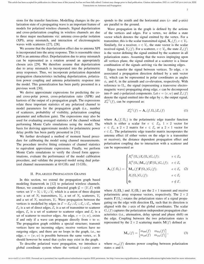
In this section, we extend the propagation graph basedmodeling framework in [12] to polarized wireless channels.Hence, we consider a simple directed graph G = (V, E) withvertex set V = Vt ∪Vs ∪Vr which is a union of three disjointsets: a set of Nt transmitters, Vt, a set of Ns scatterers, Vsand a set of Nr receivers, Vr. Wave propagation between thevertices is modelled by edges in E = Ed ∪Et ∪Es ∪Er, whereEd is a set of direct edges, Et is a set of transmitter to scattereredges, Es is a set of scatterer to scatterer edges and Er is aset of scatterer to receiver edges. An edge, e = (v, w), existsif and only if a wave can propagate directly from v to w.The propagation graph exhibits a special structure; transmitvertices have no incoming edges; receive vertices have nooutgoing edges; and there are no loops in the graph, i.e., noedge, e = (w,w) is possible between the same vertex, w. Itshould however be noted that cycles may exist in the graph.

To describe polarized wave propagation, we introduce aglobal coordinate system where the vertical (z-axis) corre-

sponds to the zenith and the horizontal axes (x- and y-axis)are parallel to the ground.

Wave propagation in the graph is defined by the actionsof the vertices and edges. For a vertex, we define a statevector which denotes the signal emitted by the vertex. For atransmitter, this is the scalar transmitted signal, Xv(f), v ∈ Vt.Similarly, for a receiver, v ∈ Vr, the state vector is the scalarreceived signal, Yv(f). For a scatterer, v ∈ Vs, the state Zv(f)is the vector defining the signal emitted by the scatterer in allpolarization states. Assuming that the waves impinging uponall vertices plane, the signal emitted at a scatterer is a linearcombination of the signals arriving via the incoming edges.

Edges transfer the signal between vertices. To edge, e isassociated a propagation direction defined by a unit vectorΩe which can be represented in polar coordinates as anglesφe and θe in the azimuth and co-elevation, respectively. Withreference to Ωe, the signal (representing a transverse electro-magnetic wave) propagating along edge, e can be decomposedinto θ- and φ-polarized components. Let e = (v, w) and Zv(f)denote the signal emitted into the edge by v, the output signal,Z

(e)w (f), can be expressed as:

Z(e)w (f) = Ae(f,Ωe)Zv(f) (1)

where Ae(f,Ωe) is the polarimetric edge transfer functionwhich is either a scalar for e ∈ Ed, 1 × 2 vector fore ∈ Et, a 2 × 2 matrix for e ∈ Es or a 2 × 1 vector fore ∈ Er. The polarimetric edge transfer matrix incorporates theantenna effect (if either vertex on the edge is a transmitteror receiver), the distance dependent propagation effect andpolarization coupling due to interaction with a scatterer andcan be represented as

Ae(f,Ωe) =

X Tt (Ωe)Xr(Ωe)Ge(f); e ∈ Ed

X Tt (Ωe)Mw(f)Γ(Ωe)Ge(f); e ∈ Et

Mw(f)Γ(Ωe)Ge(f); e ∈ Es

Xr(Ωe)Ge(f); e ∈ Er

0; e /∈ E ,

(2)

where Xt(Ωe) and Xr(Ωe) are the 2× 1 transmit and receivepolarimetric array response vectors, respectively. The 2 × 2matrix Γ(Ωe) rotates the polarization states of a signal propa-gating on the edge with direction Ωe such that its direction isaligned with the z-axis of the global coordinates. The scalarGe(f) captures the polarization-independent propagation char-acteristics (i.e., attenuation, delay spread and phase shift) onthe edge. Coupling between the two polarization states isrepresented by the 2× 2 scattering matrix M(f) defined as

Mw(f) =

[mθθ(f) mθφ(f)mφθ(f) mφφ(f)

], (3)

where mab(f) denotes power coupling between polarizationstates a and b.



3

Tx

Rx

S1

S2

S3S4

S5

S6

X tXt

X t Xt

M1X

rM3Xr

M2X r

M5

M4

M4

M6

Fig. 1: Example of a propagation graph for a polarized channel withone transmitter, one receiver and six scatterers. Blue arrow representsthe direct edges from transmitter to receiver. Black(green) and redarrows denote the transmitter(receiver) to scatterer and inter-scattereredges, respectively.

Combining (1) with the action of a vertex, the signal at theoutput of vertex, w in the graph has the form:

Zw(f) =

Xw(f); w ∈ Vt

Yw(f); w ∈ Vr∑v∈V Ae(f,Ωe)Zv(f); w ∈ Vs.

(4)

Propagation in the polarized graph can be described by a (Nt+Nr+2Ns)×(Nt+Nr+2Ns) polarimetric weighted adjacencymatrix, A(f) whose entries are the polarized edge transferfunction. A(f) is of the form,

A(f) =

0 0 0D(f) 0 R(f)T(f) 0 B(f)

, (5)

with sub-matrices:

D(f) ∈ CNr×Nt : transmitters→ receivers

T(f) ∈ C2Ns×Nt : transmitters→ scatterers

R(f) ∈ CNr×2Ns : scatterers→ receivers

B(f) ∈ C2Ns×2Ns : scatterers→ scatterers. (6)

It should be noted that although the polarimetric adjacencymatrix has the same structure as given in [12] for the uni-polarized channel, the dimension and structure of the polarizedsub-matrices differs from those in [12]. Assuming that thechannel is time-invariant, the received signal vector Y(f)reads

Y(f) = H(f)X(f), (7)

where X(f) is the transmitted signal vector and H(f) is thepolarized transfer matrix. Following a similar procedure as in[12], H(f) of the propagation graph is obtained as

H(f) = D(f) + R(f)[I−B(f)]−1T(f), (8)

provided that the spectral radius of B(f) is less than unity.

III. STOCHASTIC POLARIZED CHANNEL MODEL

The polarized propagation graph described in Section IIis valid for general edge transfer functions and scatteringmatrices. Therefore, to compute channel transfer matrices from(8), it is necessary to specify the scattering matrix, Mw(f) andedge transfer functions, Ae(f). An example of how to definethe edge transfer functions of a propagation graph for an in-room scenario assuming only specular reflections is given in[12]. We define the polarization independent component ofthe polarimetric edge transfer function based on this examplemodel and highlight the procedure for stochastic generation ofthe polarized channel in this section.

A. Models for Gains and Polarimetric Scattering Matrix

As in [12], the polarization-independent transfer function ofthe edge, e can be expressed as

Ge(f) = ge(f) exp[j(ψe − 2πτef)], (9)

where ψe and τe denote the phase and propagation delay,respectively. The edge propagation delay can be calculatedfor edge, e = (vn, vm) from the vertex position vectors, rn/mas τe = |(rm − rn)|/c, where c is the speed of light and ||denotes norm of the associated vector. The edge gain, ge(f)can be calculated from [12]

ge(f) =

1(4πfτe)

; e ∈ Ed1√

4πτ2e fµ(Et)S(Et)

; e ∈ Etg

odi(e) ; e ∈ Es1√

4πτ2e fµ(Er)S(Er)

; e ∈ Er,

(10)

Here, g denotes the reflection gain, odi(e) denotes the numberof outgoing edges from the nth scatterer,

µ(Ea) =1

|Ea|∑e⊂Ea

τe, S(Ea) =∑e⊂Ea

τ−2e , Ea ⊂ E , (11)

where | · | denotes set cardinality.We assume for simplicity that the scattering matrix is equal

for all scatterers and model the polarization transfer matrix ateach scatterer as

M =1

1 + γ

[1 γγ 1

], (12)

where γ is the polarization power coupling parameter andranges from 0 to 1.

B. Stochastic Generation of Polarized Channels

We assume that the position of all vertices lie in a boundedregion, representing the part of the propagation environmentaffecting the received signal. The transmitter and receiverlocations are assumed to be fixed and known whereas scattererpositions are drawn randomly according to a specified spatialscatterer distribution over the bounded region. The transmitter



4

Algorithm 1: Stochastic Generation of Polarized Channel

Input: Model parameters: Ns, Pvis, g, γ, fmin, fmax,∆f androom dimensions.

1: Specify the coordinates of the transmitter(s) and re-ceiver(s).

2: Draw the positions, rn of N scatterers according to thespecified spatial scatterer distribution.

3: Generate edges independently according to the edge oc-currence probability in (13).

4: Compute edge gains using (9) and polarimetric edgetransfer functions using (2).

5: Compute H(f); f = fmin, fmin + ∆f, · · · , fmax using(8)

6: Compute channel impulse response, h(τ) via inversediscrete Fourier transform.

Output: H(f); h(τ)

and receiver positions may also be drawn randomly, if desired.An edge e ∈ E is drawn with probability

Pr[e ∈ E ] =

Pdir, e ∈ EdPvis, e ∈ (Et, Es, Er)0, otherwise.

(13)

The phases ψe are drawn independently from a uniformdistribution on [0, 2π) and edge gains are computed using (5).We specify a value for the polarization coupling parameter, γand compute the scattering matrix using (12). Based on theseparameters of the graph, entries of the graph adjacency matrixare computed using (2). The polarized channel transfer func-tion is computed over the desired frequency range, [fmin, fmax]from (8). The time domain channel impulse response of thepolarized channel is then obtained via a windowed inverseFourier transform of the transfer function. The polarizedchannel generation procedure is summarized in Algorithm. 1.

IV. ANALYSIS OF THE POLARIMETRIC POWER DELAYSPECTRUM

We analyze the polarimetric power delay spectrum (PDS)1

by using an approximation and validate this approximation viasimulations. We approximate the full propagation graph by asimpler graph as shown in Fig. 2.

We consider the transmitted signal as a power pulse emittedat time, τ = 0, i.e., Pt = |X|2. For simplicity, we assume thatX(τ) = δ(τ). Ignoring the direct component, the power of thereceived signal at time τ is expressed as

Pr(τ) = GTr Ps(τ)Gt. (14)

1The power delay spectrum (PDS) is used here to denote expectation of thepower delay profile (PDP) considering the limiting case of infinite bandwidths[32], [33]. For simulated channels, the PDS is approximated by the averagedpower delay profile (APDP) obtained for a high (but finite) bandwidth signal.

Here, the vectors, Gr/t denote the receiver/transmitter polari-metric array response vector averaged over all directions andare defined as

Gt/r = [µθt/r µφt/r]T

=1

4π

∫ 2π

0

∫ π

0

Xt/r(θ, φ) sin θdθdφ, (15)

where µθt/r and µφt/r denote the θ- and φ-polarized componentof the averaged transmit/receive antenna response, respec-tively.

The power of the scattered component, Ps(τ) is approxi-mated as follows. First, we consider the mean time betweenscattering interactions, µτ . This we equate to the ratio of themean cord length of the room and speed of light, which is[32], [34],

µτ =4V

cS, (16)

where V and S are the volume and total surface area of theroom, respectively.

Consider the power received from paths arriving after k-bounces, Ps[k] which can be cast as

Ps[k] = ΥE[Nk]E[Uk], (17)

where Nk and Uk denote the number of k-bounce paths andthe power per k-bounce path, respectively. The scaling factor,Υ, accounts for the power decay during the average periodassociated with the transmitter to scatterer and scatterer toreceiver edges. Approximating the time per edge by µτ , Υ isobtained from (10) as

Υ =

(1

4πfµτ

)2

. (18)

To obtain an approximation for Ps[k], we shall approximatethe last two factors. With high Pvis, the second factor is wellapproximated as

E[Nk] ≈ PvisNs(Pvis(Ns − 1))k−1. (19)

The third factor is approximately,

E[Uk] ≈ (g2)k−1Mk

PvisNs(Pvis(Ns − 1))k, (20)

Substituting (19) and (20) into (17) yields

Ps[k] =Υ(g2)k−1Mk

Pvis(Ns − 1)(21)

The expression in (21) gives the average power level of pathsarriving after k bounces. We assume that all k-bounce paths,will on average arrive with excess delay τ = (k−1)µτ relativeto the time delay of a 1-bounce path. The number of bounceindex k can therefore be replaced with τ/µτ + 1 yielding adiscrete function Ps[τ ]; τ = 0, µτ , 2µτ , · · · . Relaxing to anyreal τ , we obtain

Ps(τ) =Υg(2τ/µτ )M(1+τ/µτ )

Pvis(Ns − 1). (22)

Substituting (22) into (14) yields

Pr(τ) = GTrΥg(2τ/µτ )M(1+τ/µτ )

Pvis(Ns − 1)Gt. (23)



5

Vt Vs VrM 1

1

g2M

Fig. 2: Simplified model for the power transfer in a graph.Labels on the edges represent power gain without delaydependent decay and antenna responses.

Inserting the eigenvalue decomposition of M and using (15)yields after some simplifications,

Pr(τ) =Υg(2τ/µτ )(µθtµ

θr + µφt µ

φr )

2Pvis(Ns − 1)

1 +

(1− γ1 + γ

)(1+τ/µτ )

+Υg(2τ/µτ )(µθtµ

φr + µφt µ

θr )

2Pvis(Ns − 1)

1−

(1− γ1 + γ

)(1+τ/µτ ).

(24)

The first and second terms of (24) are the co- and cross-polar components of the PDS, respectively. It appears that thedecay of the PDS is controlled by the average reflection gain,g and polarization mixing parameter, γ. However, the effectof γ vanishes with increasing delay. The expression in (24) isvalid for general polarimetric antenna responses. Special casesappear by inserting values for µθ/φt/r .

A. Special Case:Lossless Antennas With Perfect Cross-PolarIsolation

For a lossless antenna, the principle of conservation ofenergy implies that µθt/r + µφt/r = 1. Furthermore, withperfect cross-polar isolation, the co- and cross-polar averagedresponses become one and zero, respectively.

With Gt = [1 0]T and Gr = [1 0]T , (24) gives the co-polar PDS as

Pco(τ) =Υg(2τ/µτ )

2Pvis(Ns − 1)

1 +

(1 − γ

1 + γ

)(1+τ/µτ ). (25)

The cross-polar PDS obtained with Gt = [1 0]T and Gr =[0 1]T is

Pcro(τ) =Υg(2τ/µτ )

2Pvis(Ns − 1)

1 −

(1 − γ

1 + γ

)(1+τ/µτ ). (26)

In the region where τ µτ (i.e., tail of the PDS), the co-and cross-polar PDS decay exponentially as

Pco/cro(τ) ≈ Υg(2τ/µτ )

2Pvis(Ns − 1), (27)

The polarimetric PDS in (27) is independent of the polarizationcoupling parameter γ and shows that in the later part ofthe profile, the co- and cross-polar channels become approx-imately equal both in power level and decay rate. Based on(27), the decay rate of the PDS is then defined as

ρ ≈ 20

µτlog10(g) [dB/s]. (28)

0 20 40Delay [ns]

-135

-130

-125

-120

-115

-110

-105

-100

-95

-90

-85

Pow

er [d

B]

Co-pol:g=0.8; =0.1Cro-pol:g=0.8; =0.1Co-pol:g=0.6; =0.1Cro-pol:g=0.6; =0.1Co-pol:g =0.6; =0.2Cro-pol:g=0.6; =0.2

0 20 40Delay [ns]

0

5

10

15

20

25

Pow

er R

atio

[dB

]

= 0.1 = 0.2 = 0.5 = 0.8

Fig. 3: Dependence of channel statistics on model parametersfor a 3× 4× 3 m3 room. The LOS term is set to zero.

Thus, ρ is controlled by the average reflection gain, g and themean interaction delay, µτ .

The cross-polar power ratio, denoted here as β is obtainedfrom (25) and (26) as

β(τ) =Pco(τ)

Pcro(τ)

=1 +

(1−γ1+γ

)(1+τ/µτ )1−

(1−γ1+γ

)(1+τ/µτ ) . (29)

For τ µτ , (29) becomes one.Fig. 3 shows an example ofthe approximate power delay spectrum and cross-polarizationratio with different model parameters. As predicted by (27),the co- and cross-polar power delay spectra approach eachother with increasing delay and become nearly equal.

V. MODEL CALIBRATION

To utilize the proposed model, specific values should begiven to the parameters, Θ = [g,Ns, Pvis, γ]. Here, wecalibrate the model by estimating these parameters frommeasurements of the channel transfer function. To this end, wederive a method of moment (MoM) [35] based estimator forthe model parameters. We estimate the parameters by fittingestimated moments of the measured channel to the expressionsderived in in Section IV.

A. MoM Based Model Calibration Procedure

To calibrate the model, we fit estimates of the second mo-ments of PDS and cross-polarization ratio to the expressions(25), (26) and (29). Since Ns and Pvis are not identifiable in thePDS and cross-polarization ratio, we therefore introduced theproduct ν = (Ns − 1)Pvis as a parameter. This identifiabilityproblem can be overcome by selecting a value for eitherparameter and computing the other from the estimate ofthe product, ν. While it is advantageous for computationalcomplexity reasons to select a low value for Ns, choosing a



6

reasonable value to reproduce the scattering in a particularenvironment may be difficult. We therefore, propose settingvalue of Pvis in this paper. It is relatively straightforwardto set values of Pvis since probability values are bounded(i.e., 0 < Pvis ≤ 1) and relates intuitively to the density ofobjects in the room. Note that further work may be neededon characterizing the probability of visibility and determiningthese values for different types of propagation environment.

Given the measured channel transfer matrices H(f); f ∈[fmin fmax], we compute the impulse response h(τ); for allpolarizations and estimate the model parameters following thecalibration procedure in Algorithm 2.

Algorithm 2: MoM Based Model Calibration Procedure

Input: Measured impulse response; h(τ); τ = τmin . . . τmax

for co- and cross-polar channels and Pvis.1: Compute the PDS, Pco and Pcro and cross-polarization

ratio, β from h(τ).2.2: Estimate the decay rate, ρ from the slope of Pco and solve

(28) for g.3: Estimate the polarization mixing parameter, γ by fitting β

to (29).4: Find ν by least squares fitting of the sum of (25) and (26)

to Pco + Pcro.5: Compute Ns = ν/Pvis

Output: Model parameters: Θ = [g, Ns, Pvis, γ]

B. Verification of Approximate Polarimetric Power DelaySpectrum

We compare predictions of the power delay profile andcross-polarization ratios from the approximate expressionsto those obtained from the graph model. We consider twoscenarios in the evaluation:• Graph Model I: Transmitter and receiver locations are

fixed and equal for each realization of the propagationgraph, and

• Graph Model II: Transmitter and receiver locations arerandom and drawn uniformly within the room for eachchannel realization.

Fig. 4 reports estimated PDS and XPR obtained by averagingpower delay profiles over 1000 Monte Carlo runs with thesettings in Table II. The approximate PDS shows very goodagreement with the simulated PDS from the model for the twoscenarios. The XPR plots also show that the predicted andsimulated cross-polarization delay profile exhibits very goodagreement with a difference less than 1 dB over the entiredelay values shown.

C. Model Calibration Performance

In order to evaluate the performance of the proposed cali-bration procedure, we first test the method on simulated databefore applying the procedure on the measured data sets. Weconsider an in-room scenario with parameters in Table II anddifferent combinations of the model parameters. The numberof estimates of the PDS utilized in the calibration is set to

0 20 40Delay [ns]

-120

-115

-110

-105

-100

-95

-90

-85

Pow

er [d

B]

0 20 40Delay [ns]

0

5

10

15

20

25

Pow

er r

atio

[dB

]

Graph Model IApproximationGraph Model II

Co-pol

Cross-pol

Fig. 4: Simulated power delay profile and cross-polarizationratio from the propagation graph and approximate expressions.

TABLE I: Performance of model calibration procedure eval-uated via simulation with fixed transmitter and receiver posi-tions.

g γ ν Pvis Ns

True 0.70 0.20 12.60 0.90 15Estimate 0.72 0.20 12.46 0.90 15% Error 2.86 0.90 1.12 – 0



True 0.65 0.05 17.48 0.92 20Estimate 0.65 0.05 17.20 0.92 20% Error 0.17 0 1.60 – 0

K = 200 with τ1 = 7.75 ns and τK = 57.75 ns. The true andestimated parameters are presented in Table I. The probabilityof visibility which is chosen and number of scatterers obtainedfrom ν are included in the table for completeness. As shownin Table I, all model parameters are accurately estimatedwith calibration error less than 3 % for all parameter values.Thus, we consider the procedure to be sufficiently accurate tocalibrate the model.

VI. MEASUREMENT DATASETS

Three measurement datasets named M1, M2, and M3 areused for calibration and validation of the polarized propa-gation graph model. The three datasets summarized beloware obtained from measurement campaigns conducted at LundUniversity, Sweden, and are reported in [36] and [37].

A. 60 GHz Small Room Measurement (M1)

The dataset M1 was obtained using a VNA at 60 GHz ina 3 × 4 × 3 m3 meeting room. It is comprised of four LOSand four NLOS datasets. For each measurement location, thetransmitter and receiver has a 5×5 virtual dual polarized rect-angular array in the horizontal and vertical plane, respectively.The transmit virtual arrays are obtained by moving the virtualelement at a regular interval of 5 mm along the y− and z-axis



7

TABLE II: Measurement settings for M1, M2 and M3.

Measurement

M1 M2 M3

Room size 3× 4× 3m3 6× 10× 3m3 6× 6× 3m3

Tx height 2.35m 2.00m 1.00mRx height 1.85m 2.50m 1.00mFreq. range 58GHz− 62GHz 14.5GHz− 15.5GHz 58GHz− 62GHzNum. of freq. samples 801 801 801

TABLE III: Model parameter estimates obtained from thecalibration datasets. Ns is computed from ν with Pvis = 0.90.

Meas. g γ Ns

M1 0.64 0.06 11M2 0.65 0.26 18

from the positions shown in Fig. 5a. At the receiver, the virtualelement is moved along the x- and y-axis to form the virtualarray. The virtual arrays emulate a 25 × 25 dual polarizedMIMO system with 50× 50 antenna ports. The height of thetransmitter and receiver are 2.35 m and 1.85 m, respectively.Detailed description of M1 can be found in [36]. The datasetis divided into two groups: M1-cal (NLOS I, NLOS II andLOS I) and M1-val (NLOS IV, LOS II and LOS IV).

B. 15 GHz Large Room Measurement (M2)

The dataset M2 was obtained using a VNA at 15 GHz ina 6× 10× 3 m3 conference room. Measurements were takenusing virtual MISO system with a a 10 × 10 antenna arrayat the transmitter and a single monopole at the receiver. Thetransmitter was placed at a fixed location in the room and thereceiver was placed at different locations as shown in 5b. LOSand NLOS measurements from the four receiver locations areused in this work. The height of the transmitter and receiverare 2 m and 2.5 m, respectively. Detailed description of M2can be found in [37]. The dataset is grouped into two: M2-cal(LOS I, LOS II , NLOS II and NLOS IV) and M2-val (LOSII, LOS IV , NLOS I and NLOS III).

C. 60 GHz Medium Sized Room Measurement (M3)

The dataset M3 was obtained using a VNA at 60 GHz ina 6 × 6 × 3 m3 conference room. Measurements were takenusing the rotating antenna technique with a high directionalhorn antenna at the receiver and an omnidirectional biconicalantennna at the transmitter. The transmitter and receiver wereplaced at the locations shown in Fig. 5c with the same heightof 1 m. Measurements were taken at every 1o while thereceiver is rotated. Detailed description of M3 can be foundin [36]. Since M3 and M1 are collected at the same frequencyin similar environments, we use M3 for cross validation of themodel.

VII. MODEL VALIDATION

In this section, we validate the proposed model and ap-proximate expressions using data from the measurements de-scribed in section VI. We follow the cross-validation proceduresummarized in Fig. 6. We utilized M1-cal and M2-cal for

model calibration. With the calibration results from these twodatasets, we validate the model using M1-val, M2-val and M3.

The model parameters obtained from the calibration pro-cedure are presented in Table III. Here, we set a high valuefor the probability of visibility (i.e, Pvis = 0.9)3 since themeasurements were conducted in nearly empty rooms. Ascan be observed from Fig. 7, the measured PDS and cross-polarization ratio agree closely with the predicted values atthe estimated model parameters for both M1-cal and M2-cal.

Fig. 8 shows that the power level and tail decay of the PDSfor M1-val are accurately predicted by the model as well asthe theoretical approximation. Similar agreements between thevalidation data, propagation graph and the approximate modelare seen in the PDS plots in Fig. 9 for M2-val. We observe inFig. 8 and Fig. 9 that the measured XPR delay profile exhibitsimilar trends as the predicted ratios: a transition from a regionof decreasing polarization ratio to a region with nearly constantratio.

We now cross validate the model with M3 data set usingestimates obtained from M1. To cross-validate the model, wefirst estimate these parameters from M1 and then attemptto predict M3. Since these measurements are obtained fromrooms with different sizes, we expect that the number ofscatterers, Ns, differs. We assume that the number of scatterersis proportional to the total surface area of the room. Thus,with Ns = 11 for M1, Ns for M3 is set to 24. With theseparameters, we observe in Fig. 10 that the power level, decayrate and XPR predictions from the model agree with thoseobtained from the measurement except for a slight powerdifference in the cross-polar channel.

The stochastic graph model cannot be expected to repre-sent all features of the measured instantaneous power delayprofiles, but as we have seen, to agree well in terms of meanvalues. Nonetheless, in Fig. 11,we compare single realizationsof the model measurements in order to evaluate how wellthe model represents the behaviour of the instantaneous co-and cross-polar power delay profiles. Three realizations ofthe propagation graph are shown along with approximationand measured power delay profile for the M1 dataset. As canbe observed from Fig. 11, the power level and decay rate ofthe measured channel are well predicted by the model exceptfor few spikes in the measurements that were not capturedby the model. A plausible explanation for this is that thesefew peaks are due to the presence of very strong reflectionsfrom objects in the room which are ignored in the model. Wefurther remark that exact reproduction of the measured profilefrom the graph model may be possible by using a detailedmap and information on the materials of the environment forconstructing the propagation graph. This is, however, outsidethe scope of the present contribution.

VIII. DISCUSSION

The propagation graph model presented in this paper pro-vides a simple method for simulating the transfer function

3With fixed Pvis(Ns − 1), Pvis can be set to lower values withoutsignificantly impacting predictions from the model. Our simulations indicatethat Pvis ≥ 0.7 works well for M1 and M2.



8

0 0.5 1 1.5 2 2.5 3 3.5 4x-axis (m)

0

0.5

1

1.5

2

2.5

3

y-ax

is (

m)

Tx LOSTx NLOSRx, LOSRx, NLOSRx x-axisRx y-axis

I

II

IIIIV

IV

(a) M1.

0 2 4 6 8 10x-axis (m)

0

1

2

3

4

5

6

y-ax

is (

m)

Tx LOSTx NLOSRx, LOSRx, NLOS

III

III IV

(b) M2

0 1 2 3 4 5 6x-axis (m)

0

1

2

3

4

5

6

y-ax

is (

m)

Tx LocationRx Location

(c) M3

Fig. 5: Floor plan of the measurement setup for M1, M2 and M3.

Calibra-tion Data

ModelCalibra-tion

PGMSimula-tion

Compa-rison

ValidationData

Hcal Θ Hsim

Hv al

Fig. 6: Model validation procedure. The measurement that isgrouped into two - Hcal and Hval for model calibration andvalidation, respectively. Hsim denotes the simulated channelfrom realizations of the propagation graph with the modelparameters from the calibration stage.

as well as the impulse response of the polarized channel.Stochastic implementation of the model requires only threereal valued (reflection gain, probability of visibility and po-larization mixing parameter) and one integer valued (numberof scatterers) model parameters in addition to basic geomet-ric parameters such as dimensions of the scattering region(i.e., room dimensions for the in-room channel consideredin the simulations) and location of transmitter and receiverto accurately predict the polarimetric power delay spectrumof the channel. The model has relatively low complexity interms of both computational cost and the number of modelparameters compared to other models for polarimetric chan-nels. For example, spatial channel models (see e.g., [6], [38])typically require characterizing parameters of the distributionof a large number of multipath components and/or clusters. Itshould be noted that the propagation graph model also allowsa deterministic approach for generating the channel impulseresponse. In this case, detailed description of the environment,obtained from a map of the environment and/or an initial raytracing step may be used to construct adjacency sub-matricesfor the propagation graph.

The calibration results for the two measured rooms (M1 andM2) considered showed nearly equal values for the reflectiongain. This appears reasonable from a physical point of view,since both rooms are in the same building and most probablymade of similar materials. We therefore, expect that regardlessof room sizes and transmission frequency, the reflection gain,

0 20 40Delay [ns]

0

5

10

15

20

25

Pow

er r

atio

[dB

]

Calibration dataApproximation

0 20 40Delay [ns]

-120

-115

-110

-105

-100

-95

-90

-85

-80

Pow

er [d

B]

Co-pol

Cross-pol

(a) M1-cal.

0 50 100Delay [ns]

-5

0

5

10

15

20

X-p

ol R

atio

[dB

]

Calibration dataApproximation

0 50 100Delay [ns]

-115

-110

-105

-100

-95

-90

-85

-80

-75

-70

Pow

er [d

B]

Cross-pol

Co-pol

(b) M2-cal.

Fig. 7: Measured calibration datasets and theoretical PDS andcross-polarization ratio with model parameters in Table III.



9

0 20 40 60Delay [ns]

-120

-100

-80

-60C

o-po

l pow

er [d

B]

0 20 40 60Delay [ns]

-130

-120

-110

-100

-90

-80

Cro

ss-p

ol p

ower

[dB

]

0 10 20 30 40 50 60Delay [ns]

0

5

10

15

20

25

Pow

er r

atio

[dB

]

Validation dataGraph Model IApproximationGraph Model II

Fig. 8: Measured and averaged simulated polarimetric PDSand XPR for M1-val.

0 20 40 60 80 100Delay [ns]

-120

-100

-80

-60

Co-

pol.

Pow

er [d

B]

0 20 40 60 80 100Delay [ns]

-120

-110

-100

-90

-80

Cro

-pol

. Pow

er [d

B]

0 10 20 30 40 50 60 70 80 90 100Delay [ns]

-5

0

5

10

15

20

Pow

er r

atio

[dB

]

MeasurementGraph Model IApproximationGraph Model II

Fig. 9: Measured and averaged simulated polarimetric PDSand XPR for M2-val.

g, will be the same for rooms made of similar materials.With the same value of probability of visibility, estimated

number of scatterers is higher for the medium sized roomthan the small room. This implies that more scatterers areneeded to reproduce channel effects in larger rooms. The po-larization coupling parameter, γ obtained from the calibrationis observed to be larger for M2. While this may be dueto the increased size and/or difference in frequency, otherfactors such as polarimetric antenna properties, height andorientation of the antenna may result in significant changein the polarization behaviour of the channel and hence, thecoupling parameter. Further study is needed to characterizethe dependence of this model parameter on frequency as wellas geometrical and environmental effects.

We remark that existing works on polarization sensitivemodelling (see e.g., [6], [39] and the references therein) inclassical spatial channel modelling literature may provide basis

0 50 100Delay [ns]

-140

-120

-100

-80

-60

Co-

pol P

ower

[dB

]

0 50 100Delay [ns]

-140

-120

-100

-80

Cro

-pol

Pow

er [d

B]

0 10 20 30 40 50 60 70 80 90 100Delay [ns]

0

10

20

30

Pow

er r

atio

[dB

]

MeasurementGraph Model IApproximationGraph Model II

Fig. 10: Measured and averaged simulated polarimetric PDSand XPR for the M3 datasets with model parameters obtainedusing M1-cal.

0 10 20 30 40 50-120

-110

-100

-90

-80

0 10 20 30 40 50-120

-110

-100

-90

-80

ApproximationGraph Model IMeasurement

0 10 20 30 40 50-120

-110

-100

-90

-80

Co-

pol P

ower

[dB

]

0 10 20 30 40 50-120

-110

-100

-90

-80

Cro

-pol

Pow

er [d

B]

0 10 20 30 40 50

Delay [ns]

-120

-110

-100

-90

-80

0 10 20 30 40 50-120

-110

-100

-90

-80

Fig. 11: Realizations of the propagation graph for M1-val.



10

for characterizing the scatterer polarization coupling parameterand hence, the scattering matrix, M in terms of propagationand geometry related characteristics. This is however, non-trivial since polarization coupling is represented in thesemodels per path and not on per scatterer basis as requiredin the propagation graph.

The cross-polar power ratio is observed in measurementsand predictions by the model to be decreasing with delay andapproaches a constant in the late part of the PDS. Thus, weobserve that the model predicts a transition of the propagatingsignal from a fully polarized state to a partially and/or non-polarized state. This effect is intuitive since power is leakedfrom one polarization state to an orthogonal state duringinteraction with scatterers and hence, the ratio between the co-and cross-polar channels decreases with increasing number ofinteractions.

Although there has been very limited studies on the depen-dence of XPR on delay in recent times, similar observationshave been reported in [40], [41]. While analyzing polarimet-ric channel measurements at 1800 MHz in [40], the authorsobserved that the ratio of co- and cross-polarized channelsvaries over time. Similarly, it was found in [41] that the co-and cross-polar channels exhibit different decay constants.However, the cross-polarization ratio was shown to increasewith delay for the macrocellular environment considered. Thiscontrasting observation was noted in [6] as surprising. Forthe same macrocellular environment, the cross-polarizationratio is modelled as a decreasing function of delay in the3GPP model [7]. In a recent study based on measurementsat 63 GHz, the cross-polarization ratio is found to decreasewith increasing excess loss of the propagation paths [42]. Thisagree with our observation that the ratio decreases with delay,since propagation paths with longer delay are more likely tohave higher excess loss with respect to free space.

IX. CONCLUSION

We have presented a propagation graph based model forpolarized wireless channels in this paper. We also derivedapproximate closed form expressions for the power delayspectrum and cross polarization ratio of the indoor channelvia the propagation graph formalism. A method of momentsprocedure for calibrating the graph model using measureddata has also been presented. Our results showed that bothgraph model and theoretical approximation predicts accuratelythe power level and tail decay of the measured power delayprofile for both co- and cross-polar channels. The co- andcross-polar channels decay exponentially with different andequal decay rates in the early and later parts of the powerdelay spectrum, respectively. We observed that the measuredcross polarization ratio as a function of delay exhibit similartrend the as that obtained via simulations from the modeland theoretical approximations. A transition from polarizedto partially polarized and/or unpolarized state is observed inthe ratio.

ACKNOWLEDGMENT

This work is supported by the Cooperative ResearchProject VIRTUOSO, funded by Intel Mobile Communica-

tions, Keysight, Telenor, Aalborg University, and DenmarkInnovation Foundation. This work was performed within theframework of the COST Action CA15104 IRACON.

REFERENCES

[1] A. S. Y. Poon and D. N. C. Tse, “Degree-of-freedom gain from usingpolarimetric antenna elements,” IEEE Tran. on Info. Theory, vol. 57,no. 9, pp. 5695–5709, Sept 2011.

[2] R. G. Vaughan, “Polarization diversity in mobile communications,” IEEETrans. Veh. Technol., vol. 39, no. 3, pp. 177–186, Aug 1990.

[3] J. Song, J. Choi, S. G. Larew, D. J. Love, T. A. Thomas, and A. A.Ghosh, “Adaptive millimeter wave beam alignment for dual-polarizedMIMO systems,” IEEE Trans. Wireless Commun., vol. 14, no. 11, pp.6283–6296, Nov 2015.

[4] J. Park and B. Clerckx, “Multi-user linear precoding for multi-polarizedmassive MIMO system under imperfect CSIT,” IEEE Trans. WirelessCommun., vol. 14, no. 5, pp. 2532–2547, May 2015.

[5] X. Su, D. Choi, X. Liu, and B. Peng, “Channel model for polarizedMIMO systems with power radiation pattern concern,” IEEE Access,vol. 4, pp. 1061–1072, 2016.

[6] M. Shafi, M. Zhang, A. L. Moustakas, P. J. Smith, A. F. Molisch,F. Tufvesson, and S. H. Simon, “Polarized MIMO channels in 3D:models, measurements and mutual information,” IEEE J. Sel. AreasCommun., vol. 24, no. 3, pp. 514–527, Mar 2006.

[7] 3GPP-3GPP2, “Spatial channel model for multiple input multiple output(MIMO) simulations,” 3GPP, Tech. Rep., 2003.

[8] P. Kyosti, J. Meinila, L. Hentila, X. Zhao, T. Jamsa, C. Schneider,M. Narandzic, M. Milojevic, A. Hong, J. Ylitalo, V.-M. Holappa,M. Alatossava, R. Bultitude, Y. de Jong, and T. Rautiainen, “WINNERII Channel Models,” EC FP6, Tech. Rep., 2007.

[9] M. Zhu, G. Eriksson, and F. Tufvesson, “The COST 2100 ChannelModel: Parameterization and Validation Based on Outdoor MIMOMeasurements at 300 MHz,” 2013.

[10] T. Pedersen and B. H. Fleury, “A realistic radio channel model based instochastic propagation graphs,” in 5th Conf. on Mathematical Modelling(MATHMOD 2006), Feb. 2006, pp. 324–331.

[11] ——, “Radio channel modelling using stochastic propagation graphs,”in IEEE ICC, June 2007, pp. 2733–2738.

[12] T. Pedersen, G. Steinbock, and B. H. Fleury, “Modeling of reverber-ant radio channels using propagation graphs,” IEEE Trans. AntennasPropag., vol. 60, no. 12, pp. 5978–5988, Dec 2012.

[13] R. Zhang, X. Lu, Z. Zhong, and L. Cai, A Study on Spatial-temporalDynamics Properties of Indoor Wireless Channels, 2011, pp. 410–421.

[14] B. Uguen, N. Amiot, and M. Laaraiedh, “Exploiting the graph descrip-tion of indoor layout for ray persistency modeling in moving channel,”in EUCAP, Mar 2012, pp. 30–34.

[15] R. Adeogun, T. Pedersen, and A. Bharti, “Transfer Function Compu-tation for Complex Indoor Channels Using Propagation Graphs,” inIEEE International Symposium on Personal, Indoor and Mobile RadioCommunications, Sept. 2018, pp. 566–567.

[16] R. O. Adeogun, A. Bharti, and T. Pedersen, “An iterative transfer matrixcomputation method for propagation graphs in multi-room environ-ments,” IEEE Antennas and Wireless Propagation Letters, vol. 18, no. 4,pp. 616–620, April 2019.

[17] T. Pedersen, G. Steinbock, and B. H. Fleury, “Modeling of outdoor-to-indoor radio channels via propagation graphs,” in URSI GeneralAssembly and Scientific Symposium, Aug 2014, pp. 1–4.

[18] W. Cheng, C. Tao, L. Liu, R. Sun, and T. Zhou, “Geometrical channelcharacterization for high speed railway environments using propagationgraphs methods,” in Intern. Conf. on Adv. Comm.n Tech., Feb 2014, pp.239–243.

[19] L. Tian, V. Degli-Esposti, E. M. Vitucci, X. Yin, F. Mani, and S. X. Lu,“Semi-deterministic modeling of diffuse scattering component based onpropagation graph theory,” in IEEE PIMRC, Sept 2014, pp. 155–160.

[20] T. Zhou, C. Tao, S. Salous, Z. Tan, L. Liu, and L. Tian, “Graph-based stochastic model for high-speed railway cutting scenarios,” IETMicrowaves, Antennas Propagation, vol. 9, no. 15, pp. 1691–1697, 2015.

[21] D. K. Ntaikos, A. C. Iossifides, and T. V. Yioultsis, “Enhanced graph-theoretic channel model for performance evaluation of MIMO antennasand millimeter wave communications,” in EuCAP, May 2015, pp. 1–4.

[22] J. Chen, X. Yin, L. Tian, and M. D. Kim, “Millimeter-wave channelmodeling based on a unified propagation graph theory,” IEEE Commun.Lett., vol. 21, no. 2, pp. 246–249, Feb 2017.



11

[23] G. Steinbock, M. Gan, P. Meissner, E. Leitinger, K. Witrisal, T. Zemen,and T. Pedersen, “Hybrid model for reverberant indoor radio channelsusing rays and graphs,” IEEE Trans. Antennas Propag., vol. 64, no. 9,pp. 4036–4048, Sept 2016.

[24] L. Tian, V. Degli-Esposti, E. M. Vitucci, and X. Yin, “Semi-deterministicradio channel modeling based on graph theory and ray-tracing,” IEEETrans. Antennas Propag., vol. 64, no. 6, pp. 2475–2486, June 2016.

[25] M. Gan, G. Steinbock, Z. Xu, T. Pedersen, and T. Zemen, “A hybrid rayand graph model for simulating vehicle-to-vehicle channels in tunnels,”IEEE Transactions on Vehicular Technology, vol. 67, no. 9, pp. 7955–7968, Sept 2018.

[26] Y. Miao, T. Pedersen, M. Gan, E. Vinogradov, and C. Oestges, “Rever-berant room-to-room radio channel prediction by using rays and graphs,”pp. 1–1, 2018.

[27] V. Degli-Esposti, V. M. Kolmonen, E. M. Vitucci, and P. Vainikainen,“Analysis and modeling on co- and cross-polarized urban radio propa-gation for dual-polarized MIMO wireless systems,” vol. 59, no. 11, pp.4247–4256, Nov 2011.

[28] C. Oestges, V. Erceg, and A. J. Paulraj, “Propagation modeling of MIMOmultipolarized fixed wireless channels,” IEEE Trans. Veh. Technol.,vol. 53, no. 3, pp. 644–654, May 2004.

[29] C. Oestges, “A comprehensive model of dual-polarized channels: Fromexperimental observations to an analytical formulation,” in Third Inter-national Conference on Communications and Networking in China, Aug2008, pp. 1071–1075.

[30] R. Adeogun and T. Pedersen, “Propagation graph based model formultipolarized wireless channels,” in IEEE WCNC, April 2018.

[31] ——, “Modelling polarimetric power delay spectrum for indoor wirelesschannels via propagation graph formalism,” in 2nd URSI Atlantic RadioScience Meeting, May 2018.

[32] T. Pedersen, “Modeling of Path Arrival Rate for In-Room Radio Chan-nels With Directive Antennas,” IEEE Transactions on Antennas andPropagation, vol. 66, no. 9, pp. 4791–4805, Sep. 2018.

[33] ——, “Stochastic Multipath Model for the In-Room Radio ChannelBased on Room Electromagnetics,” IEEE Transactions on Antennas andPropagation, vol. 67, no. 4, pp. 2591–2603, April 2019.

[34] C. F. Eyring, “Reverberation time in ”dead rooms”,” American Journalof Acoustic Society, vol. 1, pp. 217 – 241, 1930.

[35] S. M. Kay, Fundamentals of Statistical Signal Processing: EstimationTheory. Upper Saddle River, NJ, USA: Prentice-Hall, Inc., 1993.

[36] C. Gustafson, D. Bolin, and F. Tufvesson, “Modeling the polarimetricmm-wave propagation channel using censored measurements,” in 2016IEEE Global Communications Conference (GLOBECOM), Dec 2016,pp. 1–6.

[37] Q. Liao, Z. Ying, and C. Gustafson, “Simulations and measurements of15 and 28 GHz indoor channels with different array configurations,” in2017 International Workshop on Antenna Technology: Small Antennas,Innovative Structures, and Applications (iWAT), March 2017, pp. 256–259.

[38] C. Gustafson, K. Haneda, S. Wyne, and F. Tufvesson, “On mm-wavemultipath clustering and channel modeling,” vol. 62, no. 3, pp. 1445–1455, March 2014.

[39] Y. I. Wu and K. T. Wong, “Polarisation-sensitive geometric modellingof the distribution of direction-of-arrival for uplink multipaths,” IETMicrowaves, Antennas Propagation, vol. 5, no. 1, pp. 95–101, January2011.

[40] M. Nilsson, B. Lindmark, M. Ahlberg, M. Larsson, and C. Beckman,“Measurements of the spatio-temporal polarization characteristics of aradio channel at 1800 MHz,” in IEEE 49th VTC, vol. 1, Jul 1999, pp.386–391 vol.1.

[41] M. Toeltsch, J. Laurila, K. Kalliola, A. F. Molisch, P. Vainikainen, andE. Bonek, “Statistical characterization of urban spatial radio channels,”2002.

[42] A. Karttunen, C. Gustafson, A. F. Molisch, J. Jrvelinen, and K. Haneda,“Censored multipath component cross-polarization ratio modeling,”IEEE Wireless Commun. Lett., vol. 6, no. 1, pp. 82–85, Feb 2017.

Polarimetric Wireless Indoor Channel Modelling Based on ... · Polarimetric Wireless Indoor Channel...

Documents

Transcript of Polarimetric Wireless Indoor Channel Modelling Based on ... · Polarimetric Wireless Indoor Channel...