2127-D03 Rev B 4/4/01

POLARIMETER OPERATING MANUAL

MODELS

PA510 / PA510-EC PA530 / PA530-EC PA550 / PA550-EC PA560 / PA560-EC

435 Route 206, P.O. Box 366, Newton, NJ 07860

SALES (973)-579-7227 : FAX 973-300-3600 www.thorlabs.com

COPYRIGHT THORLABS, INC. 1998

2

Table of Contents Section 1 – Specifications ............................................................................................................................ 4

1.1 Performance Specifications: ............................................................................................................... 4

1.2 Physical Properties: ............................................................................................................................ 4

1.3 General: .............................................................................................................................................. 4

1.4 Accessories:........................................................................................................................................ 4

Section 2 - Installing and Configuring the Polarimeter Software.................................................................. 5 2.1 Installation........................................................................................................................................... 5

2.2 Running the Program for the First Time ............................................................................................. 5

2.3 MDI Frame Window ............................................................................................................................ 5

Section 3- The User Interfaces..................................................................................................................... 7 3.1 Console Controls ................................................................................................................................ 7

Switching from Local to Remote modes ............................................................................7 3.2 Main Control Toolbar .......................................................................................................................... 7

3.3 - “Manual Adj” Control......................................................................................................................... 9

3.4 - Gain Control.................................................................................................................................... 10

3.4.1 Local Mode gain control............................................................................................11 3.5 Scope Window.................................................................................................................................. 11

3.5.1 Local Mode scope window........................................................................................11 Section 4 - System Calibration ................................................................................................................... 12

4.1 Preparing Input Polarization States .................................................................................................. 12

4.2 The System Calibration .................................................................................................................... 13

4.2.1 Remote mode calibration ..........................................................................................13 4.2.2 Local Mode calibration ..............................................................................................16

Section 5 – Display Windows ..................................................................................................................... 17 5.1 Properties Window............................................................................................................................ 17

5.1.1 Choosing a Color Scheme ........................................................................................18 5.1.2 Active Option ..............................................................................................................18 5.1.3 Auto-size Option ........................................................................................................18 5.1.4 Avr/Update Control ....................................................................................................18 5.1.5 Cancel / Reset / Defaults / OK Controls ...................................................................18

5.2 - Edit Colors Window ........................................................................................................................ 19

5.2.1 “Select Color” Control...............................................................................................19 5.2.2 Red, Green, Blue Sliders ...........................................................................................19 5.2.3 Preview On Parent .....................................................................................................19 5.2.4 “Reset Color” Control................................................................................................20 5.2.5 Cancel / Reset All / Defaults / OK .............................................................................20

3

5.3 Numerical Display Windows ............................................................................................................. 20

5.3.1 Voltages Window .......................................................................................................20 5.3.2 Stokes Window...........................................................................................................20 5.3.3 Polarization Window ..................................................................................................21 5.3.4 Ellipticity Window ......................................................................................................21

5.4 Graphical Display Windows .............................................................................................................. 21

5.4.1 Poincaré Sphere.........................................................................................................21 5.4.2 “Poincaré Sphere Properties” Window ...................................................................23 5.4.3 Polarization Ellipse ....................................................................................................25

5.5 Data Logging Windows – Data Logger............................................................................................. 26

5.6 Scope Window.................................................................................................................................. 28

5.6.1 – Layer Controls .........................................................................................................28 5.6.2 – Waterfall Plot Control .............................................................................................29 5.6.3 – Scrollbars.................................................................................................................29 5.6.4 – Scope Cursor Control.............................................................................................30 5.6.5 - Scaling Data..............................................................................................................31

Section 6 – Polarimeter Data Console ....................................................................................................... 32 Appendix A – Troubleshooting ................................................................................................................... 34 Appendix B - INI File Format ...................................................................................................................... 36

4

Section 1 – Specifications

Important Note This system can be operated in local and remote modes. When running in Local Mode a PC is not necessary to operate the system. Throughout this manual instructions will be given executing commands in local and remote modes. If there no “Local Mode” instructions located in a section this denotes that the feature is not available in Local Mode. 1.1 Performance Specifications: Operating Wavelength Range: PA510 450-700nm PA530 1100-1600nm PA550 700-900nm PA560 (Special Order) 900-1100nm Power Range: 30nW-3mW Accuracy D.O.P.: ±1.0% @ Calibrated Wavelength ±1.5% Over Operating Range 1.2 Physical Properties: Sensor: PA510 Silicon Photodiode PA530 Germanium Photodiode PA550 Silicon Photodiode PA560 Germanium Photodiode PA510/PA550 Active Area: 10 x 10mm PA530/PA560 Active Diameter: ∅5.0mm 1.3 General: Operating Voltage: 115VAC/230VAC (-EC models), 50-60Hz Operating Temperature: 10 to 40°C Size: Optical Head 31/4” x 25/8” x 31/8” Interface Box 12 ¼” x 4 1/8” x 7 5/8” 1.4 Accessories: The Polarimeter comes with the following items: 1 Optical Head 1 Polarimeter Data Console 1 Thorlabs Polarimeter Software Diskette 3 Male/Female Serial Cables 1 FC Fiber Optic Adapter 1 Polarimeter User’s Manual

5

Section 2 - Installing and Configuring the Polarimeter Software 2.1 Installation Place the provided CD-ROM into your PC’s CD-ROM drive. Open the Windows File Explorer, select the CD-ROM drive, and double-click on the file Setup.EXE. From there, follow the instructions provided by the installation software. NOTE: The head1.ini file includes calibration data that is unique to your optical head and interface box delivered along with the software CD-ROM. It is highly recommended to maintain a backup copy of this file. 2.2 Running the Program for the First Time

Now that all the necessary hardware and software have been properly installed, we’re ready for our first execution of the application. We will initiate the Polarimeter software in much the same way any software application is launched through the standard Windows environment. Select Program Files | Polar5 | Polar5. A welcome window will appear on the screen, displaying an animated Poincaré sphere as well as the revision information. If the software encounters difficulty securing a communication port, it will be indicated in a message box during this time. After the communication port is secured, the Polarimeter software will begin searching for set-up information in its working directory. If the polar.ini file is not located in the same directory as the executable code (polar5.exe) the program will not detect set-up information. A message window will appear displaying, “System Message - Default settings have been enforced.” This message is expected and no problems will arise as a result of this. Clicking “OK” will close this warning window and continue the software start-up process. Upon exiting the program, the polar.ini information file will be created. Please note, if the head1.ini file is also not present, the software will create a new head1.ini file. Some critical coefficients in the head1.ini file specific to the optical head will be set to zero. These will have to be manually adjusted if the original head1.ini file is not available. Local Mode No software installation is necessary when running the system in Local Mode. 2.3 MDI Frame Window

Now that the software has been completely loaded, the main window, called a frame window, will appear on the screen. This window is the controlling agent for all Polarimeter display windows, which are often referred to as child windows. Ultimately, the frame’s coordinates bound any child window displayed on this frame window. This means that no child window can ever be found outside the boundaries of the frame window. This boundary is not a serious limitation however. The frame window exhibits the full functionality of a Multiple Document Interface (MDI), commonly seen in word processing and database applications. The MDI frame has the ability to represent a surface area much greater than what is visible on the screen. Any children who lie either partially or completely outside the visible region of the MDI frame can be reached via horizontal and vertical scroll bars that appear on the

6

bottom and right of the frame as required. These scroll bars allow the user to pan their view port across the entire range of the frame’s virtually sized surface (defined by the extreme coordinates of the outermost child windows). This virtually expanding frame will allow the user to position the numerous children in many elaborate arrangements without being concerned with fitting the different children together like an intricate puzzle. As an added feature (discussed in Section 5) the Polarimeter software has the ability to record, in the set-up information file (polar.ini) mentioned earlier, the exact placement of children when exiting. The next time the software is executed, the layout from the previous set-up will be restored.

7

Section 3- The User Interfaces 3.1 Console Controls

Operating the system from the data console, without a PC, is referred to as “Local Mode”. While in Local Mode the keypad on the front panel of the console must be used to input data and commands (See figure below and reference Section 6 for explanation of the keypad). The arrow up, down, left, and right is used to scroll through screen options. The menu button is used to activate the main menu and also select items. When in a main menu the left arrow key can be used as a quick exit out of the menu.

Data Scope

EnterMenu

LocalEllipse

Console Key Pad Switching from Local to Remote modes Switching between modes can be done at any time. To switch between modes use the Local Key on the bottom right hand corner of the console control pad. 3.2 Main Control Toolbar

Below are descriptions of each of the buttons:

The GO button starts polling of the polarimeter.

The STOP button stops polling of the polarimeter.

If both GO and STOP buttons are inactive (grayed), refer to Appendix A - Troubleshooting.

8

SPA stands for “Samples Per Average”. When the SPA is set at one, no averaging occurs. Any number greater than one represents the number of samples averaged together for the data displayed. Local Mod The SPA can be set by pressing the menu key, scrolling down with the down arrow key and select the settings option. By pressing the ‘enter’ key again the value can now be changed by using the up/down/left/right to allow for larger values to be entered easily.

“Pk. Volts” is a visual gauge displaying the peak voltage captured by the optical head electronics. A green gauge bar indicates a good voltage level. Red indicates a voltage overload (saturation). Yellow indicates a low (but typically acceptable) voltage level. These indications represent the accuracy of the Stokes measurements whereby green suggests the best-case scenario for good measurements.

TOOLBAR TIP

The mouse with +/- symbols can be used to quickly change the value of the quantity associated with it. Move the pointer over the icon and press the left button. While holding the button down, moving the mouse up increases the value, and moving the mouse down decreases the value.

This pair of buttons manipulates Toolbar Settings. The button on the left controls the orientation of the tool bar and the button on the right controls its length. Located at the bottom of the toolbar are four status indicators. “Reading” and “Updating” Status LED’s

Used primarily to verify operation of the Main Control Loop, the status LED’s indicate the current state of the Main Control Loop, of which there are two primary operations:

Reading - acquiring voltage data Updating - updating/re-drawing display windows “Low signal” and “Bad calib” Status LED’s

During the measurement calculations, several parameters are checked to ensure the system is operating within defined limits, which assure accurate measured results. If the system is operating outside these limits, a warning indication will be displayed. The first check occurs immediately after the data acquisition routine returns voltages for analysis. If the signal is too low, the “Low signal” indicator will become illuminated red. Either increasing the gain or increasing the optical power of the incident beam can remedy this situation. Conversely, should excessive power be detected, the “Low signal” indicator will change status to “Sat. signal”, signifying that electronic saturation has been detected. The second check occurs after the calculations have been made. The measurement results are assessed to determine if the calibration constants are accurate. Calibration inaccuracy could be caused by several circumstances, many of which will be covered in Appendix A - Troubleshooting.

9

3.3 - “Manual Adj” Control

Selecting “Manual Adjustments” from the “Calibrate” menu will launch the Manual Calibration Adjustments window seen in Illustration 2. This window will allow the user to make adjustments to the calibration values while the Main Control Loop is operating. The effect of adjusting values can be seen in “real-time” during display updates. We will discuss the operation of this window in the next section. When this window is launched, four input boxes are loaded with the current system calibration values. Changing these values will effect the analysis measurements the next time the calculations are conducted, though they won’t become visible until the next time the display windows are updated. Beneath the calibration input boxes lies a separate input box labeled “Adjustment Value”. Each calibration input box has both an up and down arrow button located at its far right. Clicking the up and down arrows will increment and decrement the values in the input box by the amount specified in “Adjustment Value”, respectively. Using the up and down arrows will immediately place the new value in the measurement calculations. Manually typing new values into the input box will require the user to click the “Set” button. This button is only activated when the content of any input box is changed via the keyboard. This button will deactivate itself after it has been clicked and the new values assigned. The three remaining buttons at the bottom of the Manual Calibration Adjustments window have the following functions:

“Cancel” - will restore the calibration values to their settings prior to opening the window. This

will also close the window. “Reset” - will restore the calibration input boxes to their settings prior to opening the window.

This will not close the window “Accept” - will save the values in the input boxes as the new calibration constants.

Illustration 2 - Manual Calibration Adjustments window

10

Pitfalls Using Auto-Gain with Manual Adjustments One must pay particular attention to the gain settings prior to launching the Manual Adjustment window. The Voff value is determined by the gain combination at the time the window is opened. When “Accept” is clicked, the current DC offset value is assigned the amount specified in the Voff input box. If the gain combination changes from the time the window is launched to the time the new values are accepted, the DC offset value will be incorrectly adjusted, overriding the wrong gain combination DC offset value. IT IS HIGHLY RECOMMENDED THAT THE USER SELECT A FIXED GAIN COMBINATION RATHER THAN THE “AUTO” OPTION (DISCUSSED IN SECTION 3.3 GAIN CONTROL). 3.4 - Gain Control

To make accurate and precise measurements it is important to utilize as much of the dynamic range of the data acquisition electronics as possible. The Gain Control window allows the user to control and monitor the gain values at any time. To activate the Gain Control window select Display | Gain Control from the main menu. The Gain Control window, pictured in Illustration 3, is a versatile, visually intuitive tool used to adjust the values of the various gain stages. The main Gain Control display consists of a specialized list box that contains all the channels available to the data acquisition system via the Data Console. If this window is resized to a height that prevents viewing all the gain channels at once, a vertical scroll bar will appear in the list box, providing access to all of the entries.

Illustration 3 - Gain Control Window

Of particular interest are the first two entries in the Gain Control list box. These two entries, labeled “Polr” and “Pre”, represent the gain stages for the Polarimeter input channel and the Pre-Amp gain stage in the optical head. The selections for the pre-amp gain are coded as P1, P2, P3, and P4. These values equate to the following gain: P1 = 1X P2 = 16X P3 = 256X P4 = 4096X

11

It should also be noted that these first two entries have a right-most selection labeled “AUTO”. By selecting this option, the Polarimeter software will automatically choose the best gain combination for the incident beam power. This operation takes place each time a voltage signal is returned from the data acquisition routines while the Main Control Loop is active. The current gain selection for a given entry is indicated by a blue box with white lettering. In the case of having selected “AUTO”, the “AUTO” selection will be highlighted in blue with white lettering while the actual gain selected by the auto-gain algorithm will be highlighted in orange with white lettering. 3.4.1 Local Mode gain control Pressing the Menu button can set gain controls in Local Mode. Scroll down, select settings and press enter. Auto gain can be toggled on and off by scrolling down to “Auto Gn” and press enter. Use the arrow keys to toggle this feature on and off. Press enter again to deselect.

3.5 Scope Window

The Scope Window, activated by selecting Display | Scope from the main menu, operates much like a simplified oscilloscope. This window will display precisely the signal that is analyzed by the measurement calculations. The ability of this window to display the analyzed signal makes it invaluable for the System Calibration (Reference Section 4).

Illustration 4 - Scope Window

3.5.1 Local Mode scope window The Local Mode scope window can be selected by pressing the scope key. Vertical and Horizontal snap cursors are not available in Local Mode.

12

Section 4 - System Calibration With the knowledge of the system Toolbar and the Gain Control windows, the System Calibration may now be addressed. During the calibration routine various system parameters are characterized. These parameters include: the angles between the systems horizontal axis and the fast axis of the quarter wave plate and the linear analyzer, the optical phase retardance of the quarter wave plate at the operating wavelength, and the electronic offset voltages of the detection circuit. Attention: Each Polarimeter is calibrated at Thorlabs at a specific wavelength and at room temperature. Each polarimeter should be re-calibrated by the customer, especially under the working conditions of the application (i.e.: different wavelength or a temperature significantly warmer or cooler than room temperature). 4.1 Preparing Input Polarization States

The calibration routine is rather straightforward. In summary, it includes the following three steps:

1) The input signal must be turned off, or blocked, so that the offset voltages of the detection circuit may be measured.

2) An elliptical, near circular, state of polarization must be entered into the optical head.

3) A linear state of polarization, near horizontal, must then be entered.

Preparing these states of polarization prior to initializing the calibration routine will facilitate the calibration process. It is highly recommended that the intensities of the beams for each polarization state be approximately the same. This ensures that the gain setting will not change during calibration. One means of accomplishing this is to place a linear polarizer in the beam to generate the linear state of polarization. Then, with the linear polarizer in place, a quarter wave plate (QWP) may be added “down stream” to generate the near circular elliptical state of polarization. The only loss in intensity between the linear and near circular states is due to the Fresnel reflections and absorption (this should be minimal) associated with the QWP. Generating an Elliptical State With the horizontal polarization state set from the previous step, a quarter-wave plate may be used to generate an elliptical, near circular, state of polarization. Using the Scope window to monitor the signal, rotate the wave-plate until two cycles of a sinusoidal signal are present between points 0 and 31. This sinusoid should be approximately twice the amplitude of the sinusoid generated by the input linear state of polarization. Once this is achieved, you are ready to begin the System Calibration. Generating a Linear Horizontal State To best align the linear state of polarization with the linear analyzer in the optical head it is easiest to use the Scope Window described earlier. Open the Scope window by selecting Display | Scope from the

frame’s main menu. Click on the Toolbar and begin adjusting the “Polr” and “Pre” gain in the Gain Control (Display | Gain Control) window as required to reach a suitable signal. With the linear polarization state input to the system, rotate the linear state of polarization until the signal level reaches its minimum value. One will notice that a linear state of polarization produces four (4) cycles of a sinusoidal signal in the Scope window from point 0 to point 31 (one complete data set). One will also notice that the offset and phase of the sinusoid will vary as the linear polarization state is rotated. It will help to increase the gain until the signal is saturated and only the troughs of the signal are evident,

13

to best detect the minimum of the signal. Once this is found, rotate the linear state of polarization precisely 90 degrees. The linear state of polarization will then be aligned with the transmission axis of the linear analyzer. Select the gain combination that yields the maximum signal without signal saturation (between 8 and 9 Volts). Note: Aligning the linear horizontal polarization state to the transmission axis of the linear analyzer in the optical will yield an orientation of the linear polarization state along the horizontal axis of the optical head (perpendicular to the mounting axis) to within a few degrees. If the orientation of the linear horizontal polarization state is known and the user would like to calibrate the Polarimeter to it, this can be accomplished provided that it does not deviate from the transmission axis of the linear analyzer in the optical head by more that ±25°.

4.2 The System Calibration 4.2.1 Remote mode calibration Selecting Calibrate | System Calibration from the main menu launches the System Calibration routine. This will immediately display the calibration window, placing it in the center of the viewable screen. You’ll notice that the first of four slides of the system calibration is titled “Calibrate DC Offset”. The term 'slides' refers to the different stages of the same window. If one examines the bottom of the window, several control buttons can be seen. “Record” / ”Stop” Control Each slide in the System Calibration requires different input parameters for the incident beam. Once the proper input configuration is set, clicking the “Record” button will collect the data. This activates the data

acquisition routine that reads the number of data sets specified in the input box, then averages them and stores them for use in the calibration routine. To minimize the random noise in the data acquisition system, it is recommended that the SPA value be set between 15 and 30 Immediately after the “Record” button is clicked, the caption of this button changes to “Stop”. At the same time, all other controls on the window become temporarily deactivated. Clicking “Stop” will immediately end the data acquisition routine, which will return the averaged data up to the point of stopping. This will also re-enable the other controls (as if the data acquisition routine had completed on its own). “Previous” and “Next” Controls The flexibility of the System Calibration allows the user to click “Previous” or “Next” to traverse through the slides, viewing or using any slide. If, for example, one realizes on the last calibration slide that the DC offset voltages were recorded with the laser turned on, one may click “Previous” until they return to the “Calibrate DC Offset” slide where the data may be recorded again. Then the "Next" button may be pressed to return to the appropriate slide in the calibration routine to continue.

14

4.2.1.1 Calibrate DC Offset

To obtain accurate DC offset voltages the laser source should be turned off, or the incident beam should be interrupted (as close to the source as possible). In the first slide of the calibration window, the program will prompt the user to block the source and select the desired gain settings to read the DC offset voltages. Located in a list box labeled “Select Gain”, the four possible pre-amp gains are listed (along with their currently stored DC offset voltages). Each selection can be chosen in turn and calibrated individually with the “Record” button. In addition to the pre-amp gains, there is an "Auto" option; which is the default selection. With this option selected, clicking “Record” will cycle through each pre-amp gain with it’s corresponding four Polr settings, and will automatically and record the individual DC offset voltages. When the DC offset calibration has completed, click “Next” to continue with the calibration routine. 4.2.1.2 Calibrate Elliptical

Allow the elliptically polarized beam generated in section 4.2 to enter the optical head, and click the “Record” button to collect and average the number of data sets specified in the SPA control.

15

When the Elliptical calibration has completed, click “Next” to continue with the calibration routine. 4.2.1.3 Calibrate Horizontal

Now allow the linearly polarized beam generated in section 4.2 to enter the optical head, and click the "Record" button to collect and average the number of data sets specified in the "Samples/Average" input box. When the Horizontal calibration has completed, click “Next” to continue with the calibration routine. 4.2.1.4 Accept Values

After the horizontal state of polarization is entered, the calibration routine uses the data collected during the routine to make the calibration measurements. The final slide shows the results of the calibration. The following values are displayed: γ - the angle, in radians, between the defined horizontal and the transmission axis of the linear polarizer, δ - the angle, in radians, between the defined horizontal and the fast axis of the quarter wave plate, φ - the phase retardance of the quarter wave plate at the operating wavelength, and Voff (the displayed offset voltage is for the first pre-amp gain, P1). If these values appear to be reasonable, click “Accept”. 4.2.1.5 Save/Load Multiple Calibration Values Whenever the polarimeter is to be operated at a new wavelength, the system must be recalibrated and new calibration values recalculated. Often the user might want to use the polarimeter at multiple wavelengths, but does not want to recalibrate every time the wavelength is changed. With software version 5.0, the user has the option of saving calibration values for different wavelengths, allowing operation of the system at different wavelengths without the need to recalibrate the system each time the input wavelength is changed. After clicking on “Accept” in the final slide during the calibration routine, the user will have the option of saving the newly calculated calibration values to a file for future reference. A window will open, prompting the user to enter a file name in which to save the calibration values. The file will be saved with the .ini extension. Once the name of the file has been entered (either by typing in a new name or selecting an existing file), click on “Ok”. The new calibration constants will now be saved to the specified file, as well as appearing in the Control Console window. If the user does not save the calibration values at this time, they may do so later (assuming the unit has not been recalibrated since). To save the

16

calibration constants after the calibration routine has been completed, select at the top menu bar File | Save Calibration. The same window will open as that after the calibration routine, prompting the user to enter the filename to which the calibration values will be saved. The user can then calibrate the unit at different wavelengths, following the same procedure as above, and save the calibration values to a different file. To switch between one calibration file and another, first click on “Stop” in the Control Console (or Scope) window if the unit is running. Then select File | Load Calibration. A window will open up prompting the user to select the file containing the desired calibration values. Select the desired file and click “OK”. Then click on “Start” in the Control Console window to begin running the unit with the new calibration values. All calibration data transfers between the console and PC must be done with the PC software. To transfer the calibration select Calibration Transfer | to/from Console. Note: The current calibration constants are saved in the head1.ini file when the Polarimeter software is exited. These will be the default values the next time the Polarimeter software is started. 4.2.2 Local Mode calibration The steps for calibrating the system are the same in Local Mode as remote mode. Follow the instructions provided after selecting the calibration option from the main menu.

17

Section 5 – Display Windows To add flexibility to the display configuration, the various measurements are grouped and displayed in separate windows. The display windows may be activated/de-activated, positioned, and sized individually. It is important to note that, similar to the calibration constants, all display window configurations are saved to the polar.ini file upon exiting of the Polarimeter software. The following explains some of the common attributes associated with all display windows. Right-Button Pop-Up Menu Each Display window (those windows which are activated from the “Display” menu), has what is known as a pop-up menu associated with it. Right-clicking the mouse while the pointer lies within the window display activates this menu. In general, each window includes it's own list of options, but there are some standard options displayed in all Pop-Up windows which are listed below. Active Option The first selection on each Display window’s pop-up menu is titled “Active”. This menu item indicates whether the given window is updated during the Main Control Loop. If a check mark appears next to this menu option, each time the polarization measurements are taken, this window's contents are updated. Averages Option Each Display window contains a number known as the “Averages Per Update” (APU) value. Selecting this option will display an input window requesting the user to enter an APU value. This value indicates the number of averaged data sets to be taken prior to updating the window information. As an example, if a display window has an APU value equal to 5, the window would display only every fifth set of measurements.

NOTE: the five (5) data sets are not averaged, the values of the fifth data set are used to update the window.

Properties Option The last option on the pop-up menu is labeled “Properties”. Selecting this option will display a Properties window, which allows the user to adjust any changeable attribute of the parent window. The result of selecting this option will be described in the following section. 5.1 Properties Window Each Display window has an associated Properties window that allows the user to adjust any changeable parameter of the parent window. Properties ranging from color scheme to Main Control Loop activity can be altered within this window. Illustration 5 depicts a minimum set of properties available for any Display window. Most Display windows will contain more attributes specific to their displays. These specific adjustments will be discussed for each window. The common adjustments available to all Display windows will now be discussed.

18

Illustration 5 - Common Display Window Properties

5.1.1 Choosing a Color Scheme

All Display windows allow the user to select from a few standard color schemes. Each of these color schemes has configurable pen colors that relate to the specific display being adjusted. These adjustments can be made in the Edit Colors window discussed later. The following are the available color schemes:

Monochromatic - one background color and one drawing color

Reverse Mono - Monochromatic colors are swapped Color - Multiple colors can be used to create the display 5.1.2 Active Option

Checking this option allows the window to be updated each time information is collected and calculated

during polling (activated by clicking the button on the Toolbar). 5.1.3 Auto-size Option

Checking this option will allow the software to automatically size the window in such a way that the borders are only large enough to allow all the presentable data to be viewed on the window. In the specific cases of the Poincaré Sphere window and the Polarization Ellipse window, Auto-sizing will force the aspect ratio of the display to remain 1:1. 5.1.4 Avr/Update Control

The “Avr/Update” control specifies the reset value of the APU counter. Each time the system completes a polling cycle, each Active window will decrement their individual APU counter until a zero result is reached. At that time, the window will visually update the data it represents and reset the counter back to the value specified here. If, for example, a window APU value is ‘1’, that window will update each time a polling cycle is completed. If a value of ‘5’ is set, that window will update every fifth polling cycle.

5.1.5 Cancel / Reset / Defaults / OK Controls

Located at the bottom of every Property window are four control buttons. These buttons perform the following tasks:

19

Cancel - returns parameters to their settings prior to opening window, then closes window. Reset - returns parameters to their settings prior to opening the window without closing window Defaults - sets parameters to Thorlabs recommended values for normal operation OK - assigns parameters to values currently specified in window, then closes window. 5.2 - Edit Colors Window

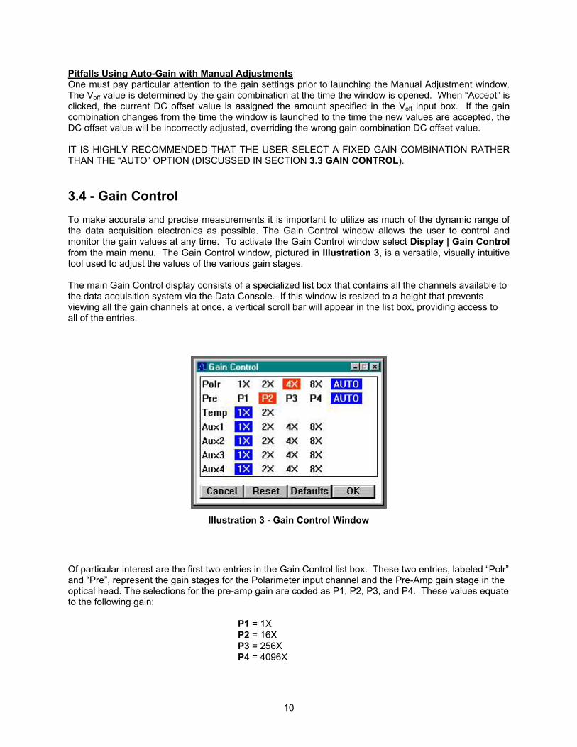
In order to add flexibility to the Display windows, the Edit Colors window allows the user to customize the drawing pens used to paint the display output. Each window will have its own specialized color schemes. Rather than discuss the specific color pens of each window, we will discuss the general functionality of the controls present on the window (reference Illustration 6).

Illustration 6 - Edit Colors Window

5.2.1 “Select Color” Control

The “Select Color” list box contains all the adjustable pen colors available to the parent window. When a color is selected from this control, the “Color Preview” box will display the current color setting. Additionally, the Red, Green, and Blue slide bars will adjust to match the color representation. 5.2.2 Red, Green, Blue Sliders

All colors displayed on a computer monitor are represented by varying the intensity of the three primary colors: red, green, and blue. By adjusting the intensity of these color components, the overall appearance of the color will change. The higher the color value, indicated by the numerical value on the right of the control, the brighter the color component. For example, a color scheme of Red = 255, Green = 0, Blue = 255 would yield a bright purple color. By contrast, the color scheme Red = 0, Green = 255, Blue = 0 would yield a bright green color. 5.2.3 Preview On Parent

Checking this option will cause the parent window to be redrawn each time a color value is adjusted. Keep in mind that only the colors belonging to the currently selected color scheme can be displayed with the “Preview on parent” option enabled. If, for example, the current color scheme for the parent window has been set to Color, adjusting the monochromatic pens will not have an effect on the display.

20

5.2.4 “Reset Color” Control

Clicking the “Reset Color” control will return the currently selected color to its value at the time the selection was made. 5.2.5 Cancel / Reset All / Defaults / OK The control buttons located at the bottom of the Edit Colors window perform the following actions:

Cancel - returns all color settings to their values prior to opening the window, then closes the window.

Reset All - returns all color settings to their values prior to opening the window, but does not close the window Defaults - assigns all color settings to values predefined by Thorlabs in the program code OK - assigns the color settings to the values specified in this window, then closes the window 5.3 Numerical Display Windows

There are four (4) Numerical Display windows. They are the Voltage, Stokes, Polarization, and Ellipticity windows. Illustration 7 depicts three of the Numerical Display windows.

Illustration 7 - Numerical Display Windows

5.3.1 Voltages Window

The largest of the display windows, the Voltages window enables the user to examine the voltages read from the optical head by the data acquisition board. The voltages displayed in the window reflect the signal after the gain stages, less the calibrated DC offset value. This window does not show much useful information as it pertains to the input polarization state, but it does allow the user to quickly identify low, and saturated, signal levels. If a user wishes to manually adjust gain values via the Gain Control window, the Voltages window, or the Scope window, can be used to assure an acceptable voltage level. 5.3.2 Stokes Window

The Stokes window enables the user to examine the normalized Stokes parameters measured during the polarization calculations. Stokes values S1, S2, and S3 reflect the coordinates of the polarization vector located on the Poincaré Sphere, which is discussed below. The S0 element can be toggled between ‘S0’ and ‘Power’ by activating ‘S0=Power’ via the ‘System’ pull-down menu. When ‘S0=Power’ is activated, the value displayed in the ‘Power’ window is raw data which may be used to assess power variations.

21

5.3.3 Polarization Window

The Polarization window enables the user to examine the varying degrees of polarization measured during the polarimetric calculations. These measurements are displayed in terms of percentage, with the labels indicating the following: DOP Degree of Polarization DOLP Degree of Linear Polarization DOCP Degree of Circular Polarization Note that the sign of the measured DOCP determines its left- or right-handedness (+ is right-handed, - is left-handed). 5.3.4 Ellipticity Window

The Ellipticity window enables the user to examine characteristics specific to the Polarization ellipse. The measurements are displayed in degrees. The following values are displayed:

Orientation Measured orientation angle of the major axis with respect to the horizontal axis (α) (in degrees)

Ellipticity Measured length ratio of the minor-to-major axes of the polarization ellipse (ω)

Local Mode In Local Mode, the Stokes vector elements and the DOPs are available in any measurement screen by pressing the data button. This will overlay the information on the current screen. 5.4 Graphical Display Windows

Two windows fall under this category; the Poincaré Sphere and Polarization Ellipse. These windows, much like the Numerical Display windows, possess all of the same functionality as described for the Display Windows. 5.4.1 Poincaré Sphere The Poincaré Sphere window is the most complex, and typically the most often viewed, of the display windows. Based on a pseudo-3D appearance, a viewer can quickly approximate the effective state of polarization exhibited by the incident beam. With the numerous adjustable parameters, the display can be modified to suit a wide range of needs. One special feature that exists only with this window is the ability to have up to five Poincaré Sphere windows open on the desktop simultaneously. This will allow the user to adjust each sphere to display a different viewing perspective in order to track varying polarization states without the need for constantly adjusting the sphere’s orientation. To gain a better understanding of this window’s versatility, the tools available directly in the Poincaré window will be described; then, the customizable parameters, found in the “Properties” and “Edit Colors” dialog boxes, will be discussed (Reference Illustration 8).

22

Illustration 8 - Poincaré Sphere Window

Rotation Located on the left, bottom, and right sides of the Poincaré Sphere window are scroll bars controlling the X-axis rotation, Y-axis rotation, and Zoom magnification respectively. By dragging the bottom scroll bar to the left and to the right rotates the Poincaré Sphere about the Y-axis. The rotation is 'real time'; it occurs as the scroll bar is moved. By dragging the left scroll bar upward and downward, the Poincaré sphere rotates about the X-axis. X-axis rotation (left scroll bar - ) rotates the sphere about a fixed X-axis. This means, no matter how the sphere is oriented, sliding the left scroll bar will rotate the sphere about an axis parallel to the bottom of the desktop. Y-axis rotation (bottom scroll bar - ) rotates the sphere about a variable Y-axis. The reason the Y-axis isn’t fixed to a parallel with the side of your desktop is because this axis is rotated along with the sphere during X-axis rotation. This phenomenon, known as gimbal lock, is a common side effect of the three-dimensional matrix rotations used by the Polarimeter software. One additional feature to note regarding these two scroll bars is the step increment buttons ( ) located at the ends of each control. These buttons allow the user to step past the range of the scroll bar. If, for example, the sphere is oriented by dragging a scrollbar all the way to one extreme of its ±360°

23

range, you can continue rotating by clicking the increment buttons. These buttons do not change the relative position of the scroll bar thumb box. Zoom The third scroll bar, located at the right of the window, is the Zoom magnifier. This slider incrementally ranges from 1X to 4X, allowing the user to zoom in on a selected focus point. There are two ways the user may select the focus point. The quickest way is to double-click the left mouse button with the mouse pointer pointing to the location of the desired focus. This causes two actions. The first is to designate the indicated location as the new focus. The second action is to magnify the current view by 40%. You’ll notice that the Zoom scroll bar adjusts position each time you double-click on a new location. The

second way to choose a focus point is to click the button located at the top of the Poincare Sphere window. When this button is clicked, the next single-click of the left mouse button inside the display area will place the focus at that spot. This is indicated by cross hairs on the display ( ). Sliding the thumb box on the Zoom slide bar will quickly illustrate the manner in which the zoom algorithm works. By progressively moving the focus point to the center of the display while increasing magnification, a smooth transition occurs between normal 1X viewing and 4X magnification. This focus location will be saved when exiting the software provided the “Save on exit” option is enabled for this window.

5.4.2 “Poincaré Sphere Properties” Window

By right-clicking inside the boundaries of the Poincaré Sphere display and selecting “Properties” from the pop-up menu, the Poincaré Sphere Properties window will appear centered on the monitor screen. Along with standard configurations, several new parameters specific to the Poincaré Sphere also appear. “Solid” Parameter Enabling this option gives the user a great sense of sphere orientation. Two important actions occur when this option is enabled. First, a border is drawn around the sphere, giving it a “solid-modeled” look. Second, the “hidden lines” (those lines which, in a solid object, would be obscured by the viewed surface) are drawn in dotted lines. “Designators” Parameter Enabling this option places polarization labels on the Poincaré sphere. These labels appear at each intersection point of the orthogonal axis. The numerical values (0, 45, 90, 135) represent linear polarization states in units of degrees. The L and R represent left and right-handed circular polarization respectively. “Vector” Parameter Enabling this option will draw a polarization vector in the Poincaré sphere, originating at the center of the sphere, and extending to the “surface” of the sphere. This vector points to the measured state of polarization as it relates to the axis of the sphere. It is important to note that the end location of the vector corresponds to the measured Stokes values with (Stokes 1, Stokes 2, Stokes 3) representing (X, Y, Z) coordinates on the sphere. The labels 0 and 90 represent the X-axis. The labels 45 and 135 represent the Y-axis. The labels L and R represent the Z-axis. For added perspective, the brightness of the vector will adjust in proportion to the viewers Z-axis. Specifically, when the vector is pointing “out of the screen”, the vector will be at its brightest, and when it points to the “back of the monitor”, the vector will be at its darkest. “Locator” Parameter As an added visual aid, the polarization state can be represented by a circular locator whose center represents the Stokes coordinates as described above. The locator can be displayed with or without the polarization vector being displayed. For added perspective, the radius and brightness of the locator will adjust in proportion to the views Z-axis, in exactly the same manner observed by the polarization vector.

24

“Locator Radius” Parameter The full-sized radius of the locator is an arbitrary value, which can easily be set in the input box labeled “Radius.” “Tracer” Parameter Enabling the Tracer option causes a 'history' line to be drawn from one polarization state to the next. This line will be continuously drawn until this option is again disabled. In order to gain better perspective on the tracer line, the brightness of the line is proportional to the viewers Z-axis, operating in exactly the same manner as the polarization vector and locator. NOTE: The software does not internally track the previous polarization states. If the Poincaré sphere window needs to be redrawn or is adjusted with its scroll bars, the tracer data is lost. Reset Values The "Reset Value" button is located at the top of the Poincaré sphere window. It looks like the Poincaré sphere. Clicking this button will set the sphere to a pre-defined orientation. That orientation is defined in the Reset Values. The X-axis and Y-axis reset values are designated in degrees ranging ±360°. The Zoom reset value ranges from 100 to 400, representing the range 1X to 4X. There is also an alternative approach to setting the default view that will be discussed below in the section titled Define Reset View. Step Values The step values represent, in degrees, the rotational increment induced by clicking the double-arrow increment buttons located at each end of the X and Y-axis rotation scroll bars. “Tracer” Pop-Up Option Selecting this option from the right mouse button’s pop-up menu will toggle the tracer on and off. When this menu item is check marked, the tracer is enabled. This has an identical effect to checking the “Tracer” parameter described above. “Define Reset View” Pop-Up Option If a particular orientation of the Poincaré sphere seems to be especially useful, selecting “Define Reset View” from the right mouse button pop-up menu will record the current orientation values. These are the same values that can be set in the “Reset Values” section of the Poincaré Sphere Properties window. One additional function of selecting this option is that the zoom focus location will also be recorded. As mentioned previously in Reset Values, clicking the “Reset View” button will always return the sphere to this newly saved orientation.

25

5.4.3 Polarization Ellipse

Illustration 9 - Polarization Ellipse Window

The “Polarization Ellipse” window graphically displays the numerical data viewed in the “Ellipticity” window. Though the Ellipticity and Polarization Ellipse windows will work independently, which means that they do not both need to be 'active' for proper operation. However, it is often useful to view them simultaneously. (Reference Illustration 9) The “Polarization Ellipse” window offers several customizable parameters affecting the graphical display. Each serves to more easily interpret the displayed information. Boundary Enabling the “Boundary” parameter will draw a circle in the display window. This circle has a radius a few pixels larger than the major axis of the polarization ellipse. This circle enables the viewer to quickly compare the polarization ellipse to the boundary. An ellipse whose ellipticity measures 1.00 would be a perfect circle, easily comparable to the boundary. Deviations from the perfect circle are visually detectable.

Boundary Fill Enabling the “Boundary fill” parameter will paint a solid boundary border, which extends to the boundaries of the parent window. With proper color selection, this option improves the visual distinction between the boundary and the polarization ellipse. Boundary Axis Checking the “Boundary Axis” parameter draws orthogonal axes through the Polarization Ellipse display. If the “Boundary” parameter is also enabled, the axis will extend only to the boundary. If no boundary is

26

present, the axis will extend to the boundaries of the parent window. This aids in visually approximating the orientation angle of the polarization ellipse’s major axis. Ellipse Axis Enabling the “Ellipse Axis” parameter draws both the major and minor axis of the polarization ellipse. These axes extend only to the boundary of the polarization ellipse. This, combined with enabling the Boundary Axis, offers the viewer more information about the orientation of the polarization ellipse. Each of the aforementioned parameters has an associated color which can be adjusted through the Edit Colors dialog box. 5.5 Data Logging Windows – Data Logger

Illustration 10 - Data Logger Window

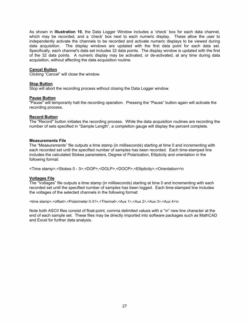
Several windows, which display measurement data in real time, have been discussed. However, these windows do not allow the user to collect measurement data over time. The Data Logging window is provided for this purpose. By collecting all the voltage and measurement data in a file, the user has the ability to import information into other software packages, such as Excel and MathCAD, to analyze and view the voltage data, or measurements. In order to capture polarization information for review in programs such as MathCAD, the Data Logger offers a suitable solution. Without interacting with any of the normal update routines, the data logger captures voltage data and polarization measurements and logs them to two distinct ASCII files. Selecting Data | Data Logger from the main menu activates the Data Logger window.

27

As shown in Illustration 10, the Data Logger Window includes a ‘check’ box for each data channel, which may be recorded, and a ‘check’ box next to each numeric display. These allow the user to independently activate the channels to be recorded and activate numeric displays to be viewed during data acquisition. The display windows are updated with the first data point for each data set. Specifically, each channel's data set includes 32 data points. The display window is updated with the first of the 32 data points. A numeric display may be activated, or de-activated, at any time during data acquisition, without affecting the data acquisition routine. Cancel Button Clicking “Cancel” will close the window. Stop Button Stop will abort the recording process without closing the Data Logger window.

Pause Button "Pause" will temporarily halt the recording operation. Pressing the “Pause” button again will activate the recording process. Record Button The "Record" button initiates the recording process. While the data acquisition routines are recording the number of sets specified in “Sample Length”, a completion gauge will display the percent complete. Measurements File The “Measurements” file outputs a time stamp (in milliseconds) starting at time 0 and incrementing with each recorded set until the specified number of samples has been recorded. Each time-stamped line includes the calculated Stokes parameters, Degree of Polarization, Ellipticity and orientation in the following format: <Time stamp>,<Stokes 0 - 3>,<DOP>,<DOLP>,<DOCP>,<Ellipticity>,<Orientation>\n Voltages File The “Voltages” file outputs a time stamp (in milliseconds) starting at time 0 and incrementing with each recorded set until the specified number of samples has been logged. Each time-stamped line includes the voltages of the selected channels in the following format: <time stamp>,<offset>,<Polarimeter 0-31>,<Thermal>,<Aux 1>,<Aux 2>,<Aux 3>,<Aux 4>\n Note both ASCII files consist of float-point, comma delimited values with a “\n” new line character at the end of each sample set. These files may be directly imported into software packages such as MathCAD and Excel for further data analysis.

28

5.6 Scope Window

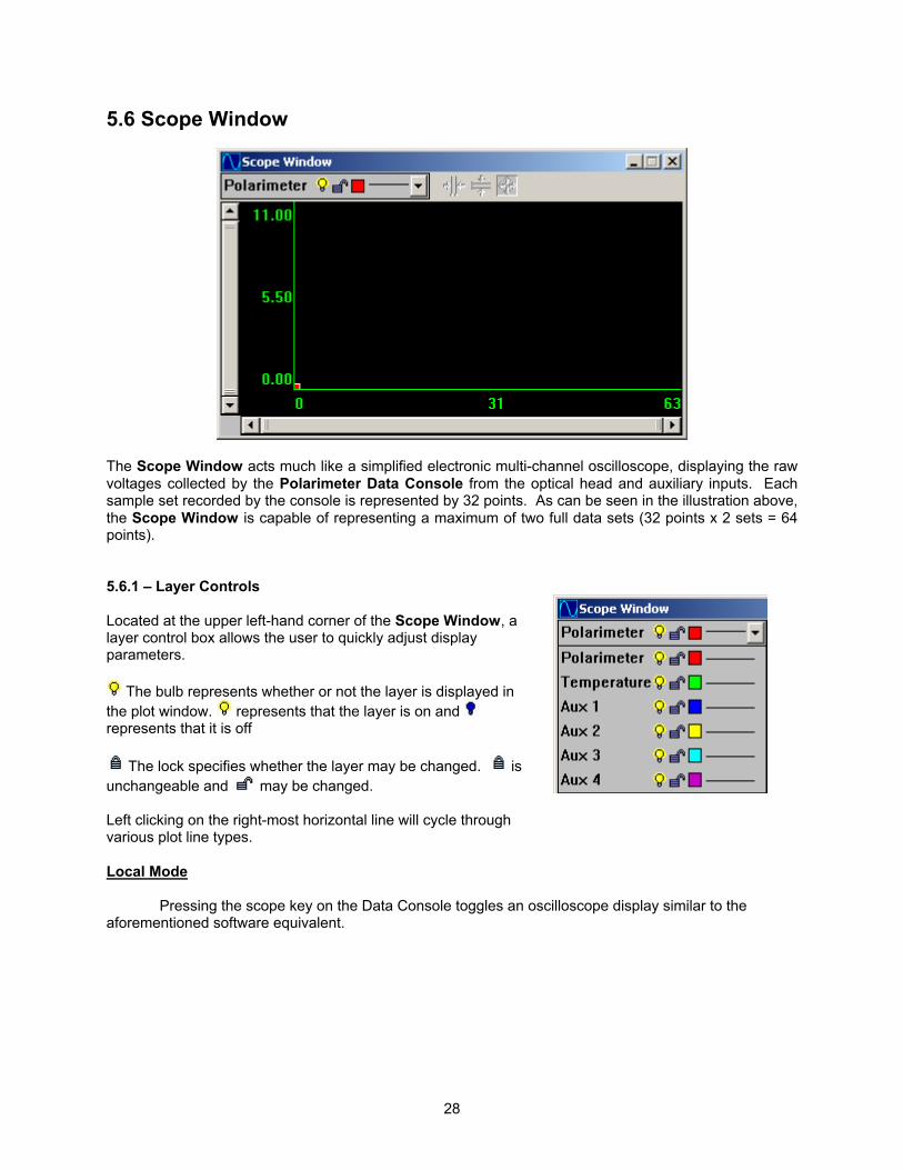
The Scope Window acts much like a simplified electronic multi-channel oscilloscope, displaying the raw voltages collected by the Polarimeter Data Console from the optical head and auxiliary inputs. Each sample set recorded by the console is represented by 32 points. As can be seen in the illustration above, the Scope Window is capable of representing a maximum of two full data sets (32 points x 2 sets = 64 points). 5.6.1 – Layer Controls Located at the upper left-hand corner of the Scope Window, a layer control box allows the user to quickly adjust display parameters.

The bulb represents whether or not the layer is displayed in the plot window. represents that the layer is on and represents that it is off

The lock specifies whether the layer may be changed. is unchangeable and may be changed. Left clicking on the right-most horizontal line will cycle through various plot line types.

Local Mode Pressing the scope key on the Data Console toggles an oscilloscope display similar to the aforementioned software equivalent.

29

Left clicking on the colored squares will activate the Color Control pop-up window. Left clicking on a colored square inside this pop-up window will select that color. Adjusting the R, G, and B sliders will adjust the red, green, and blue content of the selected colors respectively. Clicking Draw solid plot will plot each layer and fill between the plotted line and the X-axis of the display with the color depicted in the right, large color box near the bottom of this window. Left clicking the left or right large color box makes all color adjustments occur to that box. The left box indicates plot line color, the right box indicates fill color.

5.6.2 – Waterfall Plot Control

Located at the bottom left of the plot window, a small red box can be found. Placing the cursor on this control will cause the cursor to change

from to . While the cursor is in mode, hold down the left mouse button and drag the red box upwards and to the right.

As can be seen in the illustration to the right, the plot display has been stretched in such a way as to stagger the individual voltage channels. This format is typically referred to as a waterfall display. Very often it is beneficial to format the display in such a manner so as to help distinguish one channel from another.

5.6.3 – Scrollbars

Dynamic Scrollbars are used to scale the graphical output in the plot window. The image to the left shows a portion of the vertical and horizontal scrollbars. The vertical scroll bar controls the relative amplitude of the display while the horizontal scroll bar controls the span of data points displayed. Move the cursor to the end of the

vertical bar. The cursor symbol will change from to when the cursor is in a position to change the vertical scale. While in that position hold down the left mouse button and move the cursor up and down noting the change in the scale. Changes in the vertical scroll bar affect the amplitude and changes in the horizontal scroll bar affect the data set range.

30

5.6.4 – Scope Cursor Control

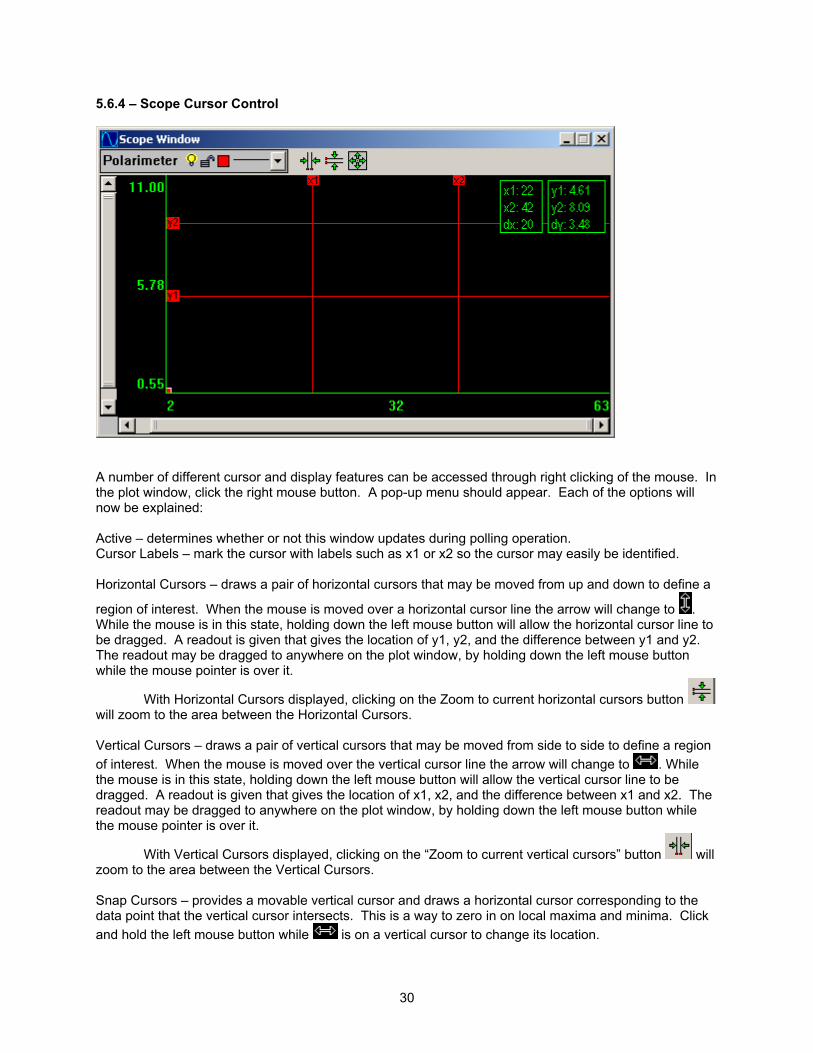
A number of different cursor and display features can be accessed through right clicking of the mouse. In the plot window, click the right mouse button. A pop-up menu should appear. Each of the options will now be explained: Active – determines whether or not this window updates during polling operation. Cursor Labels – mark the cursor with labels such as x1 or x2 so the cursor may easily be identified. Horizontal Cursors – draws a pair of horizontal cursors that may be moved from up and down to define a

region of interest. When the mouse is moved over a horizontal cursor line the arrow will change to . While the mouse is in this state, holding down the left mouse button will allow the horizontal cursor line to be dragged. A readout is given that gives the location of y1, y2, and the difference between y1 and y2. The readout may be dragged to anywhere on the plot window, by holding down the left mouse button while the mouse pointer is over it.

With Horizontal Cursors displayed, clicking on the Zoom to current horizontal cursors button will zoom to the area between the Horizontal Cursors. Vertical Cursors – draws a pair of vertical cursors that may be moved from side to side to define a region of interest. When the mouse is moved over the vertical cursor line the arrow will change to . While the mouse is in this state, holding down the left mouse button will allow the vertical cursor line to be dragged. A readout is given that gives the location of x1, x2, and the difference between x1 and x2. The readout may be dragged to anywhere on the plot window, by holding down the left mouse button while the mouse pointer is over it.

With Vertical Cursors displayed, clicking on the “Zoom to current vertical cursors” button will zoom to the area between the Vertical Cursors. Snap Cursors – provides a movable vertical cursor and draws a horizontal cursor corresponding to the data point that the vertical cursor intersects. This is a way to zero in on local maxima and minima. Click and hold the left mouse button while is on a vertical cursor to change its location.

31

Layer Plane – boxes the current layer. In the 2D view this has no effect, but in the 3D view it helps in distinguishing which layer is current and being operated on. All Solid – makes the graphical output opaque for each layer. It helps in visualization when reviewing the 3D view. In the 2D view, it acts to partially block viewing the layers behind Layer0. 5.6.5 - Scaling Data Left clicking with the curser over the numeric values and entering a new value will scale the data in the scope window. If the upper or lower value is changed, the center value will change to be centered between the upper and lower values. If the center value is changed, the range between the upper and lower values will be maintained, but they will be centered on the new center value. If the upper or lower value would be out of range (<0 or >11), then that value will clip at the limit and the total range will change to two-times the difference between the new center value and the limit. At any time, the values

may be reset to the limits by clicking the button on the menu bar of the scope window.

32

Section 6 – Polarimeter Data Console The Polarimeter Data Console operates co-operatively with the PC by means of an RS-232 interface cable supplied with this product. With a front panel keypad and LCD display, several local settings can be modified in order to best suit operating conditions. Keypad controls

Data Scope

EnterMenu

LocalEllipse

Scope – Toggle Oscilloscope Display

While in oscilloscope display, left and right arrows act as vertical scaling. Up and down arrows shift display up and down respectively. The oscilloscope display can function with or without PC polling active. Data – Toggle Numerical Display

Displays measured data returned from PC each time a polling cycle is completed. Measured parameters include S1, S2, and S3 as well as DOP, DOLP, DOCP. While in oscilloscope or ellipse displays, this option will overlay graphics and text for a more useful display. When in the remote mode, if the PC is inactive, “Remote Inactive” will flash on the screen. Ellipse – Toggle Ellipse Display

Displays polarization ellipse as described in PC version of same feature. An upper left-hand corner ‘L’ or ‘R’ display indicates “Left Circular” or “Right Circular” respectively. Left and Right arrows – Motor Speed Adjust

While in the initial utility display mode, pressing the left and right arrows will decrease and increase optical head motor speed. The current value (ranging from 0 to 240) is displayed on the utility display. Note, the lower the number indicates a faster motor speed. While in oscilloscope mode, left and right arrows decrease and increase the vertical display scaling-factor. The left arrow key can be used as a quick exit when in a menu. The right arrow key can be used to restore default settings in menu mode. Menu/Enter – Activate Menu System / Select or Accept Setting Value

While in any display mode, Menu will display the local menu system. While in the menu system, up and down arrows toggle through menu selections. Pressing the Enter button will select the currently highlighted feature. If that feature is an additional menu option, pressing

33

Enter will jump to the selected menu. If instead the feature is a setting value, the setting will be highlighted. Setting values can be changed by pressing the up and down arrows. In particular, multi-digit settings allow the user to select the individual digit to adjust by moving the cursor with the left and right arrow buttons and changing the value with the up and down arrow buttons. The following are guidelines for entering text for calibration names:

1) the ‘Data’ button will enter an ‘a’ 2) the ‘Ellipse’ button will enter an ‘A’ 3) the ‘Local’ button will enter a ‘0’ (zero) 4) the ‘Scope’ button will enter a <blank space> 5) pressing the ‘up’ button will increment the characters (e.g. ‘a’ to ‘b’ to ‘c’ …) 6) pressing the ‘down’ button will increment the characters (e.g. …‘c’ to ‘b’ to ‘a’) 7) the ‘left’ and ‘right’ buttons move the curser left and right, respectively, in the name field

34

Appendix A – Troubleshooting “System Message - Default settings have been enforced” message appears at program launch. This message is displayed when the polar.ini file is either missing from the Polarimeter working director or has been corrupted by a system crash or other mishap. In either case, the software will write a new file when the program is exited. If this is a consistent problem, check to ensure that the “Working directory” specified by the program icon matches the settings specified during installation. “Start”, “Stop”, and “Calibrate” buttons on the Control Console are disabled (grayed). During the Polarimeter initialization, which is performed each time the program is executed, the software attempts to open an RS-232 COM port. If an error occurs while attempting this communication, an error message will be displayed. Regardless of the cause, the software was unable to establish any interface with the Polarimeter Data Console. Because of this, tasks such as System Calibration and Main Control Loop execution cannot occur. For this reason, they are unavailable to the user. “Reading” and “Updating” indicators do not act in expected manner. There are several possible reasons why this might be observed. So that the potential problem might be addressed more easily, this problem has been broken down into its component symptoms. The “Reading” indicator is never illuminated. This would most likely indicate that the Main Control Loop hasn’t been initiated by clicking “Start” on the Control Console. If the “Start” button is still active (not grayed), click “Start”. The “Updating” indicator never appears to be illuminated. On very fast computers, the display updates occur so rapidly that the observer may miss the brief instant the indicator is illuminated. If one can observe the display window measurement data updating, this is most likely why the “Updating” indicator is never seen illuminated. The second cause for this behavior is if no display windows require updating. This can be caused by a lack of any display windows or a lack of Active display windows (refer to Section 5 - Active Option) The “Reading” indicator is illuminated but no display windows appear to ever update. As mentioned in the previous paragraph, one reason this would occur is if none of the display windows are Active (refer to Section 5 - Active Option). It is also possible that the Control Unit is not properly connected to either the optical head or the data console. Check to ensure that all cables are firmly connected. A final possibility is that either the optical head or the Control Unit have suffered electronic damage and are not operating properly. If this is the case, contact Thorlabs immediately. “Low signal” status indicator is illuminated. The signal resulting from the output of the gain stages minus the DC offset voltage is scanned for its peak voltage level. If that level falls below the value indicated by “LowSigTrigger” in the polar.ini file (see Appendix B). The voltage level may be heightened by increasing the values of the gain stages or increasing the optical power of the incident beam. If neither of these options is available to the operator, be aware that the measurement calculates may not yield results as accurate or precise as would normally be expected. “Bad calib” status indicator is illuminated. Among the most common causes for this indicator to become illuminated is a low voltage level (discussed in the previous paragraph). Another reason why this might occur is if incorrect, mis-aligned, or low intensity input beams were used for the System Calibration.

35

Errors occur during System Calibration. Typically this is caused by incorrect, mis-aligned, or low intensity input beams. Entering a horizontal beam when an elliptical beam is expected would certainly cause such an error. Ensure that the proper polarization states are entered at the appropriate times. Also be sure that the wavelength of the input beam falls within the range specified for the optical head. A Display window, which was present at shutdown, did not return at the next start-up. If a Display window which was present on the desktop during shutdown is not displayed at the next start-up, be sure the window’s “Save on exit” parameter is checked in its respective Properties window. Display updates occur very slowly. Typically, there are three main causes for such an occurrence. Check the value entered into the Control Console’s “Samples/Average” edit control. If this value is very high, a large number of data sets must be collected, sampled, and passed back to the Main Control Loop. Since the sample rate is fixed by the optical head, the larger the “Samples/Average” value, the longer the software must wait to make calculations and update the display windows. The second cause for this slowness could be the “APU” setting for the display windows. If these values are high, the display windows will skip several measurement sets before updating their displays. A high SPA combined with a high APU could actually make the system appear to not function at all. The final cause lies within the optical head itself. If a problem exists where the drive motor is operating at slow speeds, the data acquisition rate is proportionately slowed. If this appears to be the situation, contact Thorlabs immediately.

36

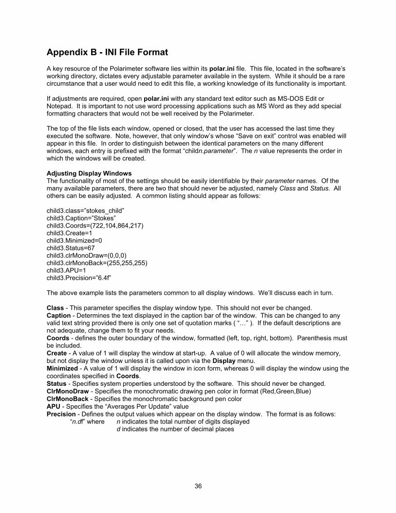
Appendix B - INI File Format A key resource of the Polarimeter software lies within its polar.ini file. This file, located in the software’s working directory, dictates every adjustable parameter available in the system. While it should be a rare circumstance that a user would need to edit this file, a working knowledge of its functionality is important. If adjustments are required, open polar.ini with any standard text editor such as MS-DOS Edit or Notepad. It is important to not use word processing applications such as MS Word as they add special formatting characters that would not be well received by the Polarimeter. The top of the file lists each window, opened or closed, that the user has accessed the last time they executed the software. Note, however, that only window’s whose “Save on exit” control was enabled will appear in this file. In order to distinguish between the identical parameters on the many different windows, each entry is prefixed with the format “childn.parameter”. The n value represents the order in which the windows will be created. Adjusting Display Windows The functionality of most of the settings should be easily identifiable by their parameter names. Of the many available parameters, there are two that should never be adjusted, namely Class and Status. All others can be easily adjusted. A common listing should appear as follows: child3.class=”stokes_child” child3.Caption=”Stokes” child3.Coords=(722,104,864,217) child3.Create=1 child3.Minimized=0 child3.Status=67 child3.clrMonoDraw=(0,0,0) child3.clrMonoBack=(255,255,255) child3.APU=1 child3.Precision=”6.4f” The above example lists the parameters common to all display windows. We’ll discuss each in turn. Class - This parameter specifies the display window type. This should not ever be changed. Caption - Determines the text displayed in the caption bar of the window. This can be changed to any valid text string provided there is only one set of quotation marks ( “…” ). If the default descriptions are not adequate, change them to fit your needs. Coords - defines the outer boundary of the window, formatted (left, top, right, bottom). Parenthesis must be included. Create - A value of 1 will display the window at start-up. A value of 0 will allocate the window memory, but not display the window unless it is called upon via the Display menu. Minimized - A value of 1 will display the window in icon form, whereas 0 will display the window using the coordinates specified in Coords. Status - Specifies system properties understood by the software. This should never be changed. ClrMonoDraw - Specifies the monochromatic drawing pen color in format (Red,Green,Blue) ClrMonoBack - Specifies the monochromatic background pen color APU - Specifies the “Averages Per Update” value Precision - Defines the output values which appear on the display window. The format is as follows: “n.df” where n indicates the total number of digits displayed d indicates the number of decimal places

37

Adjusting System Parameters At the end of the polar.ini file, a list of system parameters is defined. Most of these options should be left since they can be adjusted by the Control Console and the Gain Control window. There are, however, a few parameters adjusted so rarely that they don’t warrant attention on any standard options window. These parameters are as follows: EnableLowSignal - A value of 1 indicates the “Low signal” LED should actively monitor voltage levels, indicating to the user when problems arise. 0 disables this option. EnableBadCalib - A value of 1 indicates the “Bad calib” LED should actively monitor system calculations, indicating to the user when problems arise. 0 disables this option. LowSigTrigger - This value indicates the minimum voltage level used to compare against the inputted signal when determining whether or not the “Low signal” LED should illuminate DOP_ErrBand - When checking system calculations, a DOP value exceeding the one specified here will trigger the “Bad calib” LED to illuminate. Color.Background - This sets the background color of the software frame window in format (Red, Green, Blue).