POL 572

Multivariate Political Analysis

Gregory Wawro

Associate Professor

Department of Political Science

Columbia University

420 W. 118th St.

New York, NY 10027

phone: (212) 854-8540

fax: (212) 222-0598

email: gjw10@columbia.edu

ACKNOWLEDGEMENTS

These notes are adapted from lectures prepared by Professors Lucy Goodhart and Nolan McCarty.

The course also draws from the following works.

Baltagi, Badi H. 1995. Econometric Analysis of Panel Data. New York: John Wiley & Sons.

Beck, Nathaniel, and Jonathan N. Katz. 1995. “What To Do (and Not To Do) with Time-

SeriesCross-Section Data in Comparative Politics.” American Political Science Review 89:634-

647.

Davidson, Russell and James G. MacKinnon. 1993. Estimation and Inference in Econometrics.

New York: Oxford University Press.

Eliason, Scott R. 1993. Maximum Likelihood Estimation: Logic and Practice. Newbury Park,

CA: Sage.

Fox, John. 2002. An R and S-Plus Companion to Applied Regression. Thousand Oaks: Sage

Publications.

Greene, William H. 2003. Econometric Analysis, 5th ed. Upper Saddle River, N.J.: Prentice Hall

Gujarati, Damodar N., Basic Econometrics, 2003, Fourth Edition, New York: McGraw Hill.

Hsiao, Cheng. 1986. Analysis of Panel Data. New York: Cambridge University Press.

Kennedy, Peter. 2003. A Guide to Econometrics, Fifth Edition. Cambridge, MA: MIT Press.

King, Gary. 1989. Unifying Political Methodology. New York: Cambridge University Press

Lancaster, Tony. 1990. The Econometric Analysis of Transition Data. Cambridge: Cambridge

University Press.

Long, J. Scott. 1997. Regression Models for Categorical and Limited Dependent Variables. Thou-

sand Oaks: Sage Publications.

Maddala, G. S. 2001. Introduction to Econometrics. Third Edition, New York: John Wiley and

Sons.

ii

Wooldridge, Jeffrey M. 2002. Introductory Econometrics: A Modern Approach. Cincinnati, OH:

Southwestern College Publishing.

Wooldridge, Jeffrey M. 2002. Econometric Analysis of Cross Section and Panel Data, Cambridge,

MA: MIT Press.

iii

TABLE OF CONTENTS

LIST OF FIGURES ix

LIST OF TABLES x

I Asymptotics and Violations of Gauss-Markov Assumptions in theClassical Linear Regression Model 1

1 Large Sample Results and Asymptotics 21.1 Why do we Care about Large Sample Results (and what does this mean?) . . . . . 21.2 What are Desirable Large Sample Properties? . . . . . . . . . . . . . . . . . . . . . 41.3 How Do We Figure Out the Large Sample Properties of an Estimator? . . . . . . . 6

1.3.1 The Consistency of βOLS . . . . . . . . . . . . . . . . . . . . . . . . . . . . . 61.3.2 Asymptotic Normality of OLS . . . . . . . . . . . . . . . . . . . . . . . . . . 9

1.4 Large Sample Properties of Test Statistics . . . . . . . . . . . . . . . . . . . . . . . 111.5 Desirable Large Sample Properties of ML Estimators . . . . . . . . . . . . . . . . . 121.6 How Large Does n Have To Be? . . . . . . . . . . . . . . . . . . . . . . . . . . . . . 13

2 Heteroskedasticity 142.1 Heteroskedasticity as a Violation of Gauss-Markov . . . . . . . . . . . . . . . . . . . 14

2.1.1 Consequences of Non-Spherical Errors . . . . . . . . . . . . . . . . . . . . . 152.2 Consequences for Efficiency and Standard Errors . . . . . . . . . . . . . . . . . . . . 162.3 Generalized Least Squares . . . . . . . . . . . . . . . . . . . . . . . . . . . . . . . . 16

2.3.1 Some intuition . . . . . . . . . . . . . . . . . . . . . . . . . . . . . . . . . . 172.4 Feasible Generalized Least Squares . . . . . . . . . . . . . . . . . . . . . . . . . . . 182.5 White-Consistent Standard Errors . . . . . . . . . . . . . . . . . . . . . . . . . . . . 192.6 Tests for Heteroskedasticity . . . . . . . . . . . . . . . . . . . . . . . . . . . . . . . 20

2.6.1 Visual Inspection of the Residuals . . . . . . . . . . . . . . . . . . . . . . . . 212.6.2 The Goldfeld-Quandt Test . . . . . . . . . . . . . . . . . . . . . . . . . . . . 212.6.3 The Breusch-Pagan Test . . . . . . . . . . . . . . . . . . . . . . . . . . . . . 22

3 Autocorrelation 233.1 The Meaning of Autocorrelation . . . . . . . . . . . . . . . . . . . . . . . . . . . . . 233.2 Causes of Autocorrelation . . . . . . . . . . . . . . . . . . . . . . . . . . . . . . . . 243.3 Consequences of Autocorrelation for Regression Coefficients and Standard Errors . . 243.4 Tests for Autocorrelation . . . . . . . . . . . . . . . . . . . . . . . . . . . . . . . . . 25

3.4.1 The Durbin-Watson Test . . . . . . . . . . . . . . . . . . . . . . . . . . . . . 263.4.2 The Breusch-Godfrey Test . . . . . . . . . . . . . . . . . . . . . . . . . . . . 27

3.5 The consequences of autocorrelation for the variance-covariance matrix . . . . . . . 273.6 GLS and FGLS under Autocorrelation . . . . . . . . . . . . . . . . . . . . . . . . . 303.7 Non-AR(1) processes . . . . . . . . . . . . . . . . . . . . . . . . . . . . . . . . . . . 32

iv

3.8 OLS Estimation with Lagged Dependent Variables and Autocorrelation . . . . . . . 333.9 Bias and “Contemporaneous Correlation” . . . . . . . . . . . . . . . . . . . . . . . . 353.10 Measurement Error . . . . . . . . . . . . . . . . . . . . . . . . . . . . . . . . . . . . 353.11 Instrumental Variable Estimation . . . . . . . . . . . . . . . . . . . . . . . . . . . . 373.12 In the general case, why is IV estimation unbiased and consistent? . . . . . . . . . . 38

4 Simultaneous Equations Models and 2SLS 404.1 Simultaneous Equations Models and Bias . . . . . . . . . . . . . . . . . . . . . . . . 40

4.1.1 Motivating Example: Political Violence and Economic Growth . . . . . . . . 404.1.2 Simultaneity Bias . . . . . . . . . . . . . . . . . . . . . . . . . . . . . . . . . 41

4.2 Identifying the Endogenous Variables . . . . . . . . . . . . . . . . . . . . . . . . . . 424.3 Identification . . . . . . . . . . . . . . . . . . . . . . . . . . . . . . . . . . . . . . . 44

4.3.1 The Order Condition . . . . . . . . . . . . . . . . . . . . . . . . . . . . . . . 444.4 IV Estimation and Two-Stage Least Squares . . . . . . . . . . . . . . . . . . . . . . 45

4.4.1 Some Important Observations . . . . . . . . . . . . . . . . . . . . . . . . . . 464.5 Recapitulation of 2SLS and Computation of Goodness-of-Fit . . . . . . . . . . . . . 474.6 Computation of Standard Errors in 2SLS . . . . . . . . . . . . . . . . . . . . . . . . 484.7 Three-Stage Least Squares . . . . . . . . . . . . . . . . . . . . . . . . . . . . . . . . 504.8 Different Methods to Detect and Test for Endogeneity . . . . . . . . . . . . . . . . . 51

4.8.1 Granger Causality . . . . . . . . . . . . . . . . . . . . . . . . . . . . . . . . 514.8.2 The Hausman Specification Test . . . . . . . . . . . . . . . . . . . . . . . . . 524.8.3 Regression Version . . . . . . . . . . . . . . . . . . . . . . . . . . . . . . . . 534.8.4 How to do this in Stata . . . . . . . . . . . . . . . . . . . . . . . . . . . . . . 54

4.9 Testing for the Validity of Instruments . . . . . . . . . . . . . . . . . . . . . . . . . 54

5 Time Series Modeling 565.1 Historical Background . . . . . . . . . . . . . . . . . . . . . . . . . . . . . . . . . . 565.2 The Auto-Regressive and Moving Average Specifications . . . . . . . . . . . . . . . 56

5.2.1 An Autoregressive Process . . . . . . . . . . . . . . . . . . . . . . . . . . . . 575.3 Stationarity . . . . . . . . . . . . . . . . . . . . . . . . . . . . . . . . . . . . . . . . 585.4 A Moving Average Process . . . . . . . . . . . . . . . . . . . . . . . . . . . . . . . . 595.5 ARMA Processes . . . . . . . . . . . . . . . . . . . . . . . . . . . . . . . . . . . . . 605.6 More on Stationarity . . . . . . . . . . . . . . . . . . . . . . . . . . . . . . . . . . . 615.7 Integrated Processes, Spurious Correlations, and Testing for Unit Roots . . . . . . . 61

5.7.1 Determining the Specification . . . . . . . . . . . . . . . . . . . . . . . . . . 655.8 The Autocorrelation Function for AR(1) and MA(1) processes . . . . . . . . . . . . 655.9 The Partial Autocorrelation Function for AR(1) and MA(1) processes . . . . . . . . 665.10 Different Specifications for Time Series Analysis . . . . . . . . . . . . . . . . . . . . 675.11 Determining the Number of Lags . . . . . . . . . . . . . . . . . . . . . . . . . . . . 695.12 Determining the Correct Specification for your Errors . . . . . . . . . . . . . . . . . 705.13 Stata Commands . . . . . . . . . . . . . . . . . . . . . . . . . . . . . . . . . . . . . 71

v

II Maximum Likelihood Estimation 72

6 Intro to Maximum Likelihood 73

7 Maximum Likelihood In Depth 787.1 Asymptotic Properties of MLEs . . . . . . . . . . . . . . . . . . . . . . . . . . . . . 817.2 Iterative Process of Finding the MLE . . . . . . . . . . . . . . . . . . . . . . . . . . 84

III Models for Repeated Observations Data—Continuous Depen-dent Variables 86

8 Fixed Effects Estimators 878.1 LSDV as Fixed Effects . . . . . . . . . . . . . . . . . . . . . . . . . . . . . . . . . . 878.2 Application: Economic growth in 14 OECD countries . . . . . . . . . . . . . . . . . 93

9 Random Effects Estimators 979.1 Intro . . . . . . . . . . . . . . . . . . . . . . . . . . . . . . . . . . . . . . . . . . . . 979.2 Deriving the random effects estimator . . . . . . . . . . . . . . . . . . . . . . . . . . 989.3 GLS Estimation . . . . . . . . . . . . . . . . . . . . . . . . . . . . . . . . . . . . . . 1009.4 Maximum Likelihood Estimation . . . . . . . . . . . . . . . . . . . . . . . . . . . . 1049.5 Fixed v. Random Effects . . . . . . . . . . . . . . . . . . . . . . . . . . . . . . . . . 1059.6 Testing between Fixed and Random Effects . . . . . . . . . . . . . . . . . . . . . . 1059.7 Application . . . . . . . . . . . . . . . . . . . . . . . . . . . . . . . . . . . . . . . . 107

10 Non-Spherical Errors 10910.1 Introduction . . . . . . . . . . . . . . . . . . . . . . . . . . . . . . . . . . . . . . . . 10910.2 The Method of PCSEs . . . . . . . . . . . . . . . . . . . . . . . . . . . . . . . . . . 10910.3 Robust Estimation of Asymptotic Covariance Matrices . . . . . . . . . . . . . . . . 11110.4 Costs of ignoring unit effects revisited . . . . . . . . . . . . . . . . . . . . . . . . . . 11510.5 Heteroskedasticity in FE and RE models . . . . . . . . . . . . . . . . . . . . . . . . 11810.6 Serial Correlation in RE and FE models . . . . . . . . . . . . . . . . . . . . . . . . 12010.7 Robust standard error estimation with unit effects . . . . . . . . . . . . . . . . . . . 122

10.7.1 Arellano robust standard errors . . . . . . . . . . . . . . . . . . . . . . . . . 12210.7.2 Kiefer robust standard errors . . . . . . . . . . . . . . . . . . . . . . . . . . 123

10.8 Application: Garrett data . . . . . . . . . . . . . . . . . . . . . . . . . . . . . . . . 124

IV Qualitative and Limited Dependent Variable Models Based onthe Normal Regression Model 128

11 Introduction 12911.1 Linear Regression Model . . . . . . . . . . . . . . . . . . . . . . . . . . . . . . . . . 129

vi

12 Probit 13012.1 Interpretation of Coefficients . . . . . . . . . . . . . . . . . . . . . . . . . . . . . . . 13212.2 Goodness of fit measures . . . . . . . . . . . . . . . . . . . . . . . . . . . . . . . . . 13412.3 Voting Behavior Example . . . . . . . . . . . . . . . . . . . . . . . . . . . . . . . . 13612.4 Obstruction and Passage of Legislation Example . . . . . . . . . . . . . . . . . . . . 14012.5 Heteroskedasticity and the Probit Model . . . . . . . . . . . . . . . . . . . . . . . . 143

13 Ordered Probit 146

14 Censored Regression 15114.1 Reparameterization for tobit model . . . . . . . . . . . . . . . . . . . . . . . . . . . 15614.2 Marginal Effects . . . . . . . . . . . . . . . . . . . . . . . . . . . . . . . . . . . . . . 15914.3 Heteroskedasticity and the tobit model . . . . . . . . . . . . . . . . . . . . . . . . . 161

15 Truncated Regression 16215.1 Marginal Effects . . . . . . . . . . . . . . . . . . . . . . . . . . . . . . . . . . . . . . 164

16 Sample and Self-Selection Models 165

V Probabilistic Choice Models 177

17 Introduction 178

18 The Multinomial Logit Model 17918.1 Identification Issue . . . . . . . . . . . . . . . . . . . . . . . . . . . . . . . . . . . . 18018.2 Normalization . . . . . . . . . . . . . . . . . . . . . . . . . . . . . . . . . . . . . . . 181

19 The Conditional Logit Model 18419.1 Equivalence of the MNL model and conditional logit model . . . . . . . . . . . . . . 18719.2 Independence of Irrelevant Alternatives . . . . . . . . . . . . . . . . . . . . . . . . . 18819.3 IIA test . . . . . . . . . . . . . . . . . . . . . . . . . . . . . . . . . . . . . . . . . . 191

20 The Nested Logit Model 192

21 The Multinomial Probit Model 19521.1 Identification of variance-covariance matrix . . . . . . . . . . . . . . . . . . . . . . . 19721.2 Application: Alvarez and Nagler “Economics, Issues, and the Perot Candidacy:

Voter Choice in the 1992 Presidential Election” ’95 AJPS . . . . . . . . . . . . . . . 198

VI Duration Models 202

22 Introduction 203

vii

23 Functions for Analyzing Duration Data 204

24 Proportional Hazard Model 212

25 Partial Likelihood Estimator 214

26 Nonparametric Approaches 217

VII Event Count Models 219

27 Introduction 220

28 Poisson Regression Model 22128.1 Dispersion . . . . . . . . . . . . . . . . . . . . . . . . . . . . . . . . . . . . . . . . . 22328.2 Tests for Overdispersion . . . . . . . . . . . . . . . . . . . . . . . . . . . . . . . . . 225

29 Gamma Model for Overdispersion 227

30 Binomial Model for Underdispersion 229

31 Generalized Event Count Model 231

32 Hurdle Poisson Models 234

VIII Models for Repeated Observations—Dichotomous DependentVariables 236

33 Introduction 23733.1 Fixed Effect Logit . . . . . . . . . . . . . . . . . . . . . . . . . . . . . . . . . . . . . 23933.2 Random Effects Probit . . . . . . . . . . . . . . . . . . . . . . . . . . . . . . . . . . 24233.3 Correlated Random Effects Probit . . . . . . . . . . . . . . . . . . . . . . . . . . . . 24533.4 CRE Probit Application: PAC contributions and roll call votes . . . . . . . . . . . . 248

34 Binary Time-Series Cross-Section (BTSCS) Data 252

35 Generalized Estimating Equations (GEEs) 25635.1 GLMs for Correlated Data . . . . . . . . . . . . . . . . . . . . . . . . . . . . . . . . 25735.2 Options for specifying within-cluster correlation . . . . . . . . . . . . . . . . . . . . 25835.3 “Robust” Standard Errors . . . . . . . . . . . . . . . . . . . . . . . . . . . . . . . . 25935.4 GEE2 . . . . . . . . . . . . . . . . . . . . . . . . . . . . . . . . . . . . . . . . . . . 26035.5 Application: Panel Decision-making on the Court of Appeals . . . . . . . . . . . . . 261

viii

LIST OF FIGURES

7.1 The Natural Log of the Normal Distribution . . . . . . . . . . . . . . . . . . . . . . 85

12.1 Simulated Probabilities of Passage and Coalition Size . . . . . . . . . . . . . . . . . 142

13.1 Probabilities for categories . . . . . . . . . . . . . . . . . . . . . . . . . . . . . . . . 148

14.1 Censoring . . . . . . . . . . . . . . . . . . . . . . . . . . . . . . . . . . . . . . . . . 15214.2 Censoring and OLS . . . . . . . . . . . . . . . . . . . . . . . . . . . . . . . . . . . . 15314.3 Marginal Effects and Censoring . . . . . . . . . . . . . . . . . . . . . . . . . . . . . 160

19.1 PDF and CDF for Extreme Value Distribution . . . . . . . . . . . . . . . . . . . . . 186

23.1 Plots of hazard functions . . . . . . . . . . . . . . . . . . . . . . . . . . . . . . . . . 20623.2 Lognormal Hazard Function (λ = .5) . . . . . . . . . . . . . . . . . . . . . . . . . . 207

ix

LIST OF TABLES

10.1 Results from Monte Carlo experiments involving time invariant variables . . . . . . 117

12.1 Probability of Voting for the Incumbent Member of Congress . . . . . . . . . . . . . 13812.2 Marginal Effects on Probability of Voting for the Incumbent Member of Congress . 13912.3 Probit analysis of passage of obstructed measures, 1st–64th Congresses . . . . . . . 14112.4 Simulated Probabilities of Passage and Coalition Sizes, 1st–64th Congresses . . . . . 141

23.1 Distributions, Hazard Functions, and Survival Functions . . . . . . . . . . . . . . . 205

35.1 GEE analysis of judges’ votes in Appeals Court decisions . . . . . . . . . . . . . . . 262

x

1

Part I

Asymptotics and Violations ofGauss-Markov Assumptions in theClassical Linear Regression Model

Section 1

Large Sample Results and Asymptotics

1.1 Why do we Care about Large Sample Results (and

what does this mean?)

• Large sample results for any estimator, θ, are the properties that we can sayhold true as the number of data points, n, used to estimate θ becomes “large.”

• Why do we care about these large sample results? We have an OLS modelthat, when the Gauss-Markov assumptions hold, has desirable properties.Why would we ever want to rely on the more difficult mathematical proofsthat involve the limits of estimators as n becomes large?

• Recall to mind the Gauss-Markov assumptions:

1. The true model is a linear functional form of the data: y = Xβ + ε.

2. E[ε|X] = 0

3. E[εε′|X] = σ2I

4. X is n× k with rank k (i.e., full column rank)

5. ε|X ∼ N [0, σ2I]

• Recall that if we are prepared to make a further, simplifying assumption, thatX is fixed in repeated samples, then the expectations conditional on X canbe written in unconditional form.

• There are two main reasons for the use of large sample results, both of whichhave to do with violations of these of these assumptions.

1. Errors are not distributed normally

– If assumption 5, above, does not hold, then we cannot use the smallsample results.

– We can establish that βOLS is unbiased and “best linear unbiasedestimator” without any recourse to the normality assumption and wealso established that the variance of βOLS = σ2(X′X)−1.

2

3

– Used normality to show that βOLS ∼ N(β, σ2(X′X)−1) and that (n−k)s2/σ2 ∼ χ2

n−k where the latter involved showing that (n − k)s2/σ2

can also be expressed as a quadratic form of ε/σ which is distributedstandard normal.

– Both of these results were used to show that we could calculate teststatistics that were distributed as t and F . It is these results ontest statistics, and our ability to perform hypothesis tests, that areinvalidated if we cannot assume that the true errors are normallydistributed.

2. Non-linear functional forms

– We may be interested in estimating non-linear functions of the originalmodel.

– E.g., suppose that you have an unbiased estimator, π∗ of

π = 1/(1− β)

but you want to estimate β. You cannot simply use (1− 1/π∗) as anunbiased estimate β∗ of β.

– To do so, you would have to be able to prove that E(1−1/π∗) = β. Itis not true, however, that the expected value of a non-linear functionof π is equal to the non-linear function of the expected value of π(this fact is also known as “Jensen’s Inequality”).

– Thus, we can’t make the last step that we would require (in smallsamples) to show that our estimator of β is unbiased. As Kennedysays, “the algebra associated with finding (small sample) expectedvalues can become formidable whenever non-linearities are involved.”This problem disappears in large samples.

– The models for discrete and limited dependent variables that we willdiscuss later in the course involve non-linear functions of the param-eters, β. Thus, we cannot use the G-M assumptions to prove thatthese estimates are unbiased. However, ML estimates have attrac-tive large sample properties. Thus, our discussion of the properties ofthose models will always be expressed in terms of large sample results.

4

1.2 What are Desirable Large Sample Properties?

• Under finite sample conditions, we look for estimators that are unbiased andefficient (i.e., have minimum variance for any unbiased estimator). We havealso found it useful, when calculating test statistics, to have estimators thatare normally distributed. In the large sample setting, we look for analogousproperties.

• The large sample analog to unbiasedness is consistency. An estimator β isconsistent if it converges in probability to β, that is if its probability limit asn becomes large is β (plim β = β).

• The best way to think about this is that the sampling distribution of βcollapses to a spike around the true β.

• Two Notions of Convergence

1. “Convergence in probability”:

XnP→ X iff limn→∞ Pr(|X(ω)−Xn(ω)| ≥ ε) = 0

where ε is some small positive number. Or

plim Xn(ω) = X(ω)

2. “Convergence in quadratic mean or mean square”: If Xn has mean µn

and variance σ2n such that limn→∞µn = c and limn→∞σ

2n = 0, then Xn

converges in mean square to c.

Note: convergence in quadratic mean implies convergence in probability

(Xnqm→ c⇒ Xn

P→ c).

• An estimator may be biased in small samples but consistent. For example,take an estimate of β = β + 1/n. In small samples this is biased, but as thesample size becomes infinite, 1/n goes to zero (limn→∞ 1/n = 0).

5

• Although an estimator may be biased yet consistent, it is very hard (readimpossible) for it to be unbiased but inconsistent. If β is unbiased, there isnowhere for it to collapse to but β. Thus, the only way an estimator couldbe unbiased but inconsistent is if its sampling distribution never collapses toa spike around the true β.

• We are also interested in asymptotic normality. Even though an estimatormay not be distributed normally in small samples, we can usually appeal tosome version of the central limit theorem (see Greene, Fifth Edition, Ap-pendix D.2.6 or Kennedy Appendix C) to show that it will be distributednormally in large samples.

• More precisely, the different versions of the central limit theorem state thatthe mean of any random variable, whatever the distribution of the underlyingvariable, will in the limit be distributed such that:

√n(xn − µ)

d−→ N [0, σ2]

Thus, even if xi is not distributed normal, the sampling distribution of theaverage of an independent sample of the xi’s will be distributed normal.

• To see how we arrived at this result, begin with the variance of the mean:var(xn) = σ2

n .

• Next, by the CLT, this will be distributed normal: xn ∼ N(µ, σ2

n )

• As a result,xn − µ

σ√n

=√n

(xn − µ)

σ∼ N(0, 1)

Multiplying the expression above by σ will get you the result on the asymp-totic distribution of the sample average.

• When it comes to establishing the asymptotic normality of estimators, wecan usually express that estimator in the form of an average, as a sum ofvalues divided by the number of observations n, so that we can then applythe central limit theorem.

6

• We are also interested in asymptotic efficiency. An estimator is asymptoti-cally efficient if it is consistent, asymptotically normally distributed, and hasan asymptotic covariance matrix that is not larger than the asymptotic co-variance matrix of any other consistent, asymptotically normally distributedestimator.

• We will rely on the result that (under most conditions) the maximum like-lihood estimator is asymptotically efficient. In fact, it attains the smallestpossible variance, the Cramer-Rao lower bound, if that bound exists. Thus,to show that any estimator is asymptotically efficient, it is sufficient to showthat the estimator in question either is the maximum likelihood estimate orhas identical asymptotic properties.

1.3 How Do We Figure Out the Large Sample Properties

of an Estimator?

• To show that any estimator of any quantity, θ, is consistent, we have to showthat plim θ = θ. The means of doing so is to show that any bias approacheszero as n becomes large and the variance in the sampling distribution alsocollapses to zero.

• To show that θ is asymptotically normal, we have to show that its samplingdistribution can be expressed as the sampling distribution of a sample averagepre-multiplied by

√n.

• Let’s explore the large sample properties of βOLS w/o assuming that ε ∼N(0, σ2I).

1.3.1 The Consistency of βOLS

• Begin with the expression for βOLS:

βOLS = β + (X′X)−1X′ε

• Instead of taking the expectation, we now take the probability limit:

plim βOLS = β + plim (X′X)−1X′ε

7

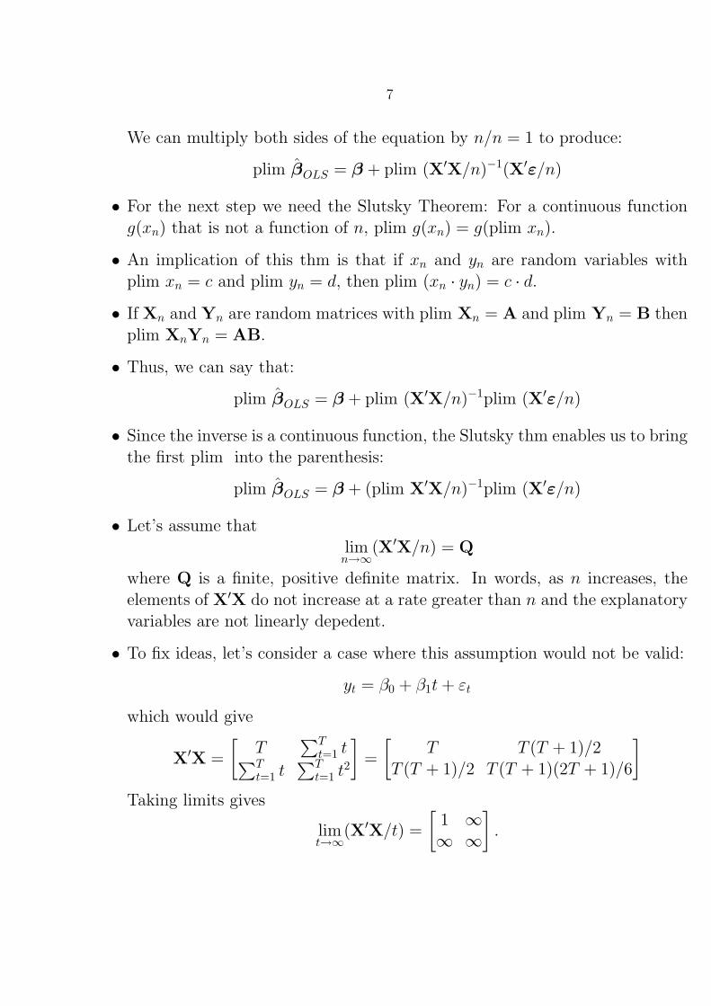
We can multiply both sides of the equation by n/n = 1 to produce:

plim βOLS = β + plim (X′X/n)−1(X′ε/n)

• For the next step we need the Slutsky Theorem: For a continuous functiong(xn) that is not a function of n, plim g(xn) = g(plim xn).

• An implication of this thm is that if xn and yn are random variables withplim xn = c and plim yn = d, then plim (xn · yn) = c · d.

• If Xn and Yn are random matrices with plim Xn = A and plim Yn = B thenplim XnYn = AB.

• Thus, we can say that:

plim βOLS = β + plim (X′X/n)−1plim (X′ε/n)

• Since the inverse is a continuous function, the Slutsky thm enables us to bringthe first plim into the parenthesis:

plim βOLS = β + (plim X′X/n)−1plim (X′ε/n)

• Let’s assume thatlimn→∞

(X′X/n) = Q

where Q is a finite, positive definite matrix. In words, as n increases, theelements of X′X do not increase at a rate greater than n and the explanatoryvariables are not linearly depedent.

• To fix ideas, let’s consider a case where this assumption would not be valid:

yt = β0 + β1t+ εt

which would give

X′X =

[T

∑Tt=1 t∑T

t=1 t∑T

t=1 t2

]=

[T T (T + 1)/2

T (T + 1)/2 T (T + 1)(2T + 1)/6

]Taking limits gives

limt→∞

(X′X/t) =

[1 ∞∞ ∞

].

8

• More generally, each element of (X′X) is composed of the sum of squares andthe sum of cross-products of the explanatory variables. As such, the elementsof (X′X) grow larger with each additional data point, n.

• But if we assume the elements of this matrix do not grow at a rate fasterthan n and the columns of X are not linear dependent, then dividing by n,gives convergence to a finite number.

• We can now say that plim βOLS = β + Q−1plim (X′ε/n) and the next stepin the proof is to show that plim (X′ε/n) is equal to zero. To demonstratethis, we will prove that its expectation is equal to zero and that its varianceconverges to zero.

• Think about the individual elements in (X′ε/n). This is a k × 1 matrix inwhich each element is the sum of all n observations of a given explanatoryvariable multiplied by each realization of the error term. In other words:

1

nX′ε =

1

n

n∑i=1

xiεi =1

n

n∑i=1

wi = w (1.1)

where w is a k × 1 vector of the sample averages of xkiεi. (Verify this if it isnot clear to you.)

• Since we are still assuming that X is non-stochastic, we can work throughthe expectations operator to say that:

E[w] =1

n

n∑i=1

E[wi] =1

n

n∑i=1

xiE[εi] =1

nX′E[ε] = 0 (1.2)

In addition, using the fact that E[εε′] = σ2I we can say that:

var[w] = E[ww′] =1

nX′E[εε′]X

1

n=σ2

n

X′X

n

• In the limit, as n→∞, σ2

n → 0, X′Xn → Q, and thus

limn→∞

var[w] = 0 ·Q

9

• Therefore, we can say that w converges in mean square to 0 ⇒ plim (X′ε/n)is equal to zero, so that:

plim βOLS = β + Q−1 · 0 = β

Thus, the OLS estimator is consistent as well as unbiased.

1.3.2 Asymptotic Normality of OLS

• Let’s show that the OLS estimator, βOLS, is also asymptotically normal. Startwith

βOLS = β + (X′X)−1X′ε

and then subtract β from each side and multiply through by√n to yield (use√

n = n/√n):

√n(βOLS − β) =

(X′X

n

)−1(1√n

)X′ε

We’ve already established that the first term on the right-hand side converges

to Q−1. We need to derive the limiting distribution of the term(

1√n

)X′ε.

• From equations 1.1 and 1.2, we can write(1√n

)X′ε =

√n(w− E[w])

and then find the limiting distribution of√nw.

• To do this, we will use a variant of the CLT (called Lindberg-Feller), whichallows for variables to come from different distributions.

From above, we know that

w =1

n

n∑i=1

xiεi

which means w is the average of n indepedent vectors xiεi with means 0 andvariances

var[xiεi] = σ2xix′i = σ2Qi

10

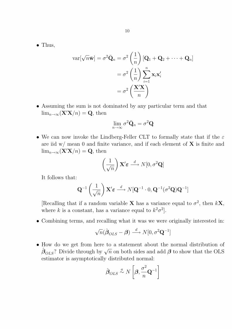
• Thus,

var[√nw] = σ2Qn = σ2

(1

n

)[Q1 + Q2 + · · ·+ Qn]

= σ2(

1

n

) n∑i=1

xix′i

= σ2(

X′X

n

)• Assuming the sum is not dominated by any particular term and that

limn→∞(X′X/n) = Q, then

limn→∞

σ2Qn = σ2Q

• We can now invoke the Lindberg-Feller CLT to formally state that if the εare iid w/ mean 0 and finite variance, and if each element of X is finite andlimn→∞(X′X/n) = Q, then(

1√n

)X′ε

d−→ N [0, σ2Q]

It follows that:

Q−1(

1√n

)X′ε

d−→ N [Q−1 · 0,Q−1(σ2Q)Q−1]

[Recalling that if a random variable X has a variance equal to σ2, then kX,where k is a constant, has a variance equal to k2σ2].

• Combining terms, and recalling what it was we were originally interested in:

√n(βOLS − β)

d−→ N [0, σ2Q−1]

• How do we get from here to a statement about the normal distribution ofβOLS? Divide through by

√n on both sides and add β to show that the OLS

estimator is asymptotically distributed normal:

βOLSa∼ N

[β,σ2

nQ−1

]

11

• To complete the steps, we can also show that s2 = e′en−k is consistent for σ2.

Thus, s2(X′X)/n)−1 is consistent for σ2Q−1. As a result, a consistent estimate

for the asymptotic variance of βOLS(= σ2

n Q−1 = σ2

n

(X′X

n

)−1) is s2(X′X)−1.

• Thus, we can say that βOLS is normally distributed and a consistent estimateof its asymptotic variance is given by s2(X′X)−1, even when the error termsare not distributed normally. We have gone through the rigors of large sampleproofs in order to show that in large samples OLS retains desirable propertiesthat are similar to what it has in small sample when all of the G–M conditionshold.

• To conclude, the desirable properties of OLS do not rely on the assumptionthat the true error term is normally distributed. We can appeal to largesample results to show that the sampling distribution will still be normalas the sample size becomes large and that it will have variance that can beconsistently estimated by s2(X′X)−1.

1.4 Large Sample Properties of Test Statistics

• Given the normality results and the consistent estimate of the asymptoticvariance given by s2(X′X)−1, hypothesis testing proceeds almost as normal.Hypotheses on individual coefficients can still be estimated by constructinga t-statistic:

βk − βk

SE(βk)

• When we did this in small samples, we made clear that we had to use an

estimate,√s2(X′X)−1

kk for the true standard error in the denominator, equal

to√σ2(X′X)−1

kk .

12

• As the sample size becomes large, we can replace this estimate by its prob-ability limit, which is the true standard error, so that the denominator justbecomes a constant. When we do so, we have a normally distributed randomvariable in the numerator divided by a constant, so the test-statistic is dis-tributed as z, or standard normal. Another way to think of this intuitively isthat the t-distribution converges to the z distribution as n becomes large.

• Testing joint hypothesis also proceeds via constructing an F -test. In this case,we recall the formula for an F -test, put in terms of the restriction matrix:

F [J, n−K] =(Rb− q)′[R(X′X)−1R′]−1(Rb− q)/J

s2

• In small samples, we had to take account of the distribution of s2 itself. Thisgave us the ratio of two chi-squared random variables, which is distributedF .

• In large samples, we can replace s2 by its probability limit, σ2 which is justa constant value. Multiplying both sides by J , we now have that the teststatistic JF is composed of a chi-squared random variable in the numeratorover a constant, so the JF statistic is the large sample analog of the F -test.If the JF statistic is larger than the critical value, then we can say that therestrictions are unlikely to be true.

1.5 Desirable Large Sample Properties of ML Estimators

• Recall that MLEs are consistent, asymptotically normally distributed, andasymptotically efficient, in that they always achieve the Cramer-Rao lowerbound, when this bound exists.

• Thus, MLEs always have desirable large sample properties although theirsmall sample estimates (as of σ2) may be biased.

• We could also have shown that OLS was going to be consistent, asymptoticallynormally distributed, and asymptotically efficient by indicating that OLS isthe MLE for the classical linear regression model.

13

1.6 How Large Does n Have To Be?

• Does any of this help us if we have to have an infinity of data points before wecan attain consistency and asymptotic normality? How do we know how manydata points are required before the sampling distribution of βOLS becomesapproximately normal?

• One way to check this is via Monte Carlo studies. Using a non-normal dis-tribution for the error terms, we simulate draws from a distribution of themodel y = Xβ + ε, using a different set of errors each time.

• We then calculate the βOLS from repeated samples of size n and plot thesedifferent sample estimates βOLS on a histogram.

• We gradually enlarge n, checking how large n has to be in order to give us asampling distribution that is approximately normal.

Section 2

Heteroskedasticity

2.1 Heteroskedasticity as a Violation of Gauss-Markov

• The third of the Gauss-Markov assumptions is that E[εε′] = σ2In. Thevariance-covariance matrix of the true error terms is structured as:

E(εε′) =

E(ε21) E(ε1ε2) . . . E(ε1εN)

... . . . ...E(εNε1) E(εNε2) . . . E(ε2

N)

=

σ2 0 ... 00 σ2 ... 0...0 0 ... σ2

• If all of the diagonal terms are equal to one another, then each realization

of the error term has the same variance, and the errors are said to be ho-moskedastic. If the diagonal terms are not the same, then the true error termis heteroskedastic.

• Also, if the off-diagonal elements are zero, then the covariance between dif-ferent error terms is zero and the errors are uncorrelated. If the off-diagonalterms are non-zero, then the error terms are said to be auto-correlated and theerror term for one observation is correlated with the error term for anotherobservation.

• When the third assumption is violated, the variance-covariance matrix of theerror term does not take the special form, σ2In, and is generally written,instead as σ2Ω. The disturbances in this case are said to be non-sphericaland the model should then be estimated by Generalized Least Squares, whichemploys σ2Ω rather than σ2In.

14

15

2.1.1 Consequences of Non-Spherical Errors

• The OLS estimator, βOLS, is still unbiased and (under most conditions) con-sistent.

Proof for Unbiasedness:

As before:βOLS = β + (X′X)−1X′ε

and we still have that E[ε|X] = 0, thus we can say that E(βOLS

)= β.

• The estimated variance of βOLS is E[(β − E(β))(β − E(β))′], which we canestimate as:

var(βOLS) = E[(X′X)−1X′εε′X(X′X)−1]

= (X′X)−1X′(σ2Ω)X(X′X)−1

= σ2(X′X)−1(X′ΩX)(X′X)−1

• Therefore, if the errors are normally distributed,

βOLS ∼ N [β, σ2(X′X)−1(X′ΩX)X′X)−1]

• We can also use the formula we derived in the lecture on asymptotics to showthat βOLS is consistent.

plim βOLS = β + Q−1plim (X′ε/n)

To show that plim (X′ε/n)=0, we demonstrated that the expectation of(X′ε/n) was equal to zero and that its variance was equal to σ2

nX′X

n , whichbecomes zero as n grows to infinity.

• In the case where E[εε′] = σ2Ω, the variance of (X′ε/n) is equal to σ2

n(X′ΩX)

n .

So long as this matrix converges to a finite matrix, then βOLS is also consistentfor β.

• Finally, in most cases, βOLS is asymptotically normally distributed with meanβ and its variance-covariance matrix is given by σ2(X′X)−1(X′ΩX)(X′X)−1.

16

2.2 Consequences for Efficiency and Standard Errors

• So what’s the problem with using OLS when the true error term may beheteroskedastic? It seems like it still delivers us estimates of the coefficientsthat have highly desirable properties.

• The true variance of βOLS is no longer σ2(X′X)−1, so that any inference basedon s2(X′X)−1 is likely to be “misleading”.

• Not only is the wrong matrix used, but s2 may be a biased estimator of σ2.

• In general, there is no way to tell the direction of bias, although Goldberger(1964) shows that in the special case of only one explanatory variable (inaddition to the constant term), s2 is biased downward if high error variancescorrespond with high values of the independent variable.

• Whatever the direction of the bias, we should not use the standard equationfor the standard errors in hypothesis tests on βOLS.

• More importantly, OLS is no longer efficient, since another method calledGeneralized Least Squares will give estimates of the regression coeffi-cients, βGLS, that are unbiased and have a smaller variance.

2.3 Generalized Least Squares

• We assume, as we always do for a variance matrix, that Ω is positive definiteand symmetric. Thus, it can be factored into a set of matrices containing itscharacteristic roots and vectors.

Ω = CΛC′

• Here the columns of C contain the characteristic vectors of Ω and Λ is adiagonal matrix containing its characteristic roots. We can “factor” Ω usingthe square root of Λ, or Λ1/2, which is a matrix containing the square rootsof the characteristic roots on the diagonal.

• Then, if T = CΛ1/2, TT′ = Ω. The last result holds because TT′ =CΛ1/2Λ1/2C′ = CΛC′ = Ω. Also, if we let P′ = CΛ−1/2, then P′P = Ω−1.

17

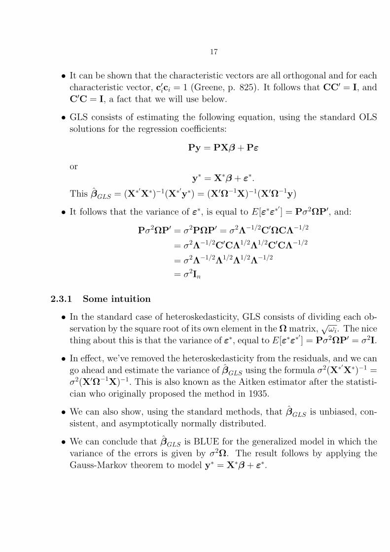
• It can be shown that the characteristic vectors are all orthogonal and for eachcharacteristic vector, c′ici = 1 (Greene, p. 825). It follows that CC′ = I, andC′C = I, a fact that we will use below.

• GLS consists of estimating the following equation, using the standard OLSsolutions for the regression coefficients:

Py = PXβ + Pε

ory∗ = X∗β + ε∗.

This βGLS = (X∗′X∗)−1(X∗′y∗) = (X′Ω−1X)−1(X′Ω−1y)

• It follows that the variance of ε∗, is equal to E[ε∗ε∗′] = Pσ2ΩP′, and:

Pσ2ΩP′ = σ2PΩP′ = σ2Λ−1/2C′ΩCΛ−1/2

= σ2Λ−1/2C′CΛ1/2Λ1/2C′CΛ−1/2

= σ2Λ−1/2Λ1/2Λ1/2Λ−1/2

= σ2In

2.3.1 Some intuition

• In the standard case of heteroskedasticity, GLS consists of dividing each ob-servation by the square root of its own element in the Ω matrix,

√ωi. The nice

thing about this is that the variance of ε∗, equal to E[ε∗ε∗′] = Pσ2ΩP′ = σ2I.

• In effect, we’ve removed the heteroskedasticity from the residuals, and we cango ahead and estimate the variance of βGLS using the formula σ2(X∗′X∗)−1 =σ2(X′Ω−1X)−1. This is also known as the Aitken estimator after the statisti-cian who originally proposed the method in 1935.

• We can also show, using the standard methods, that βGLS is unbiased, con-sistent, and asymptotically normally distributed.

• We can conclude that βGLS is BLUE for the generalized model in which thevariance of the errors is given by σ2Ω. The result follows by applying theGauss-Markov theorem to model y∗ = X∗β + ε∗.

18

• In this general case, the maximum likelihood estimator will be the GLS esti-mator, βGLS, and that the Cramer-Rao lower bound for the variance of βGLS

is given by σ2(X′Ω−1X)−1.

2.4 Feasible Generalized Least Squares

• All of the above assumes that Ω is a known matrix, which is usually not thecase.

• One option is to estimate Ω in some way and to use Ω in place of Ω in theGLS model above. For instance, one might believe that the true error termwas a function of one (or more) of the independent variables. Thus,

εi = γ0 + γ1xi + ui

• Since βOLS is consistent and unbiased for β, we can use the OLS residualsto estimate the model above. The procedure is that we first estimate theoriginal model using OLS, and then use the residuals from this regression toestimate Ω and

√ωi.

• We then transform the data using these estimates, and use OLS again onthe transformed data to estimate βGLS and the correct standard errors forhypothesis testing.

• One can also use the estimated errors terms from the last stage to conductFGLS again and keep on doing this until the error model begins to converge,so that the estimated residuals barely change as one moves through the iter-ations.

• Some examples:

– If σ2i = σ2x2

i , we would divide all observations through by xi.

– If σ2i = σ2xi, we would divide all observations through by

√xi.

– If σ2i = σ2(γ0 + γ1Xi + ui), we would divide through all observations by√

γ0 + γ1xi.

19

• Essential Result: So long as our estimate of Ω is consistent, the FGLSestimator will be consistent and will be asymptotically efficient.

• Problem: Except for the simplest cases, the finite-sample properties and ex-act distributions of FGLS estimators are unknown. Intuitively, var(βFGLS) 6=var(βGLS) because we also have to take into account the uncertainty in es-timating Ω. Since we cannot work out the small sample distribution, wecannot even say that βFGLS is unbiased in small samples.

2.5 White-Consistent Standard Errors

• If you can find a consistent estimator for Ω, then go ahead and perform FGLSif you have a large number of data points available.

• Otherwise, and in most cases, analysts estimate the regular OLS model anduse “White-consistent standard errors”, which are described by Leamer as“White-washing heteroskedasticity”.

• White’s heteroskedasticity consistent estimator of the variance-covariancematrix of βOLS is recommended whenever OLS estimates are being usedfor inference in a situation in which heteroskedasticity is suspected, but theresearcher is unable to consistently estimate Ω and use FGLS.

• White’s method consists of finding a consistent estimator for the true OLSvariance below:

var[βOLS] =1

n

(1

nX′X

)−1(1

nX′[σ2Ω]X

)(1

nX′X

)−1

• The trick to White’s estimation of the asymptotic variance-covariance matrixis to recognize that what we need is a consistent estimator of:

Q∗ =σ2X′ΩX

n=

1

n

n∑i=1

σ2i xix

′i

20

• Under very general conditions

S0 =1

n

n∑i=1

e2ixix

′i

(which is a k× k matrix with k(k+ 1)/2 original terms) is consistent for Q∗.(See Greene p. 198)

• Because βOLS is consistent for β, we can show that White’s estimate ofvar[βOLS] is consistent for the true asymptotic variance.

• Thus, without specifying the exact nature of the heteroskedasticity, we canstill calculate a consistent estimate of var[βOLS] and use this in the normalway to derive standard errors and conduct hypothesis tests. This makes theWhite-consistent estimator extremely attractive in a wide variety of situa-tions.

• The White heteroskedasticity consistent estimator is

Est. asy. var[βOLS] =1

n

(1

nX′X

)−1(

1

n

n∑i=1

e2ixix

′i

)(1

nX′X

)−1

= n (X′X)−1

S0 (X′X)−1

• Adding the robust qualifier to the regression command in Stata producesstandard errors computed from this estimated asymptotic variance matrix.

2.6 Tests for Heteroskedasticity

• Homoskedasticity implies that the error variance will be the same acrossdifferent observations and should not vary with X, the independent variables.

• Unsurprisingly, all tests for heteroskedasticity rely on checking how far theerror variances for different groups of observations depart from one another,or how precisely they are explained by the explanatory variables.

21

2.6.1 Visual Inspection of the Residuals

• Plot them and look for patterns (residuals against fitted values, residualsagainst explanatory vars).

2.6.2 The Goldfeld-Quandt Test

• The Goldfeld-Quandt tests consists of comparing the estimated error vari-ances for two groups of observations.

• First, sort the data points by one of the explanatory variables (e.g., countrysize). Then run the model separately for the two groups of countries.

• If the true errors are homoskedastic, then the estimated error variances forthe two groups should be approximately the same.

• We estimate the true error variance by s2g = (e′geg)/(ng − k), where the sub-

script g indicates that this is the value for each group. Since each estimatederror variance is distributed chi-squared, the test statistic below is distributedF .

• If the true error is homoskedastic, the statistic will be approximately equalto one. The larger the F -statistic, the less likely it is that the errors arehomoskedastic. It should be noted that the formulation below is computedassuming that the errors are higher for the first group.

e′1e1/(n1 − k)

e′2e2/(n2 − k)= F [n1 − k, n2 − k]

• It has also been suggested that the test-statistic should be calculated usingonly the first and last thirds of the data points, excluding the middle sectionof the data, to sharpen the test results.

22

2.6.3 The Breusch-Pagan Test

• The main problem w/ Goldfeld-Quandt: requires knowledge of how to sortthe data points.

• The Breusch-Pagan test uses a different approach to see if the error variancesare systematically related to the independent variables, or to any subset ortransformation of those variables.

• The idea behind the test is that for the regression

σ2i = σ2f(α0 +α′zi)

where zi is a vector of independent variables, if α = 0 then the errors arehomoskedastic.

• To perform the test, regress e2i/(e

′e/n− 1) on some combination of the inde-pendent variables (zi).

• We then compute a Lagrange Multiplier statistic as the regression sum ofsquares from that regression divided by 2. That is,

SSR

2

a∼ χ2m−1,

where m is the number of explanatory variables in the auxiliary regression.

• Intuition: if the null hypothesis of no heteroskedasticity is true, then the SSRshould equal zero. A non-zero SSR is telling us that e2

i/(e′e/n − 1) varies

with the explanatory variables.

• Note that this test depends on the fact that βOLS is consistent for β, andthat the errors from an OLS regression of yi on xi, ei will be consistent for εi.

Section 3

Autocorrelation

3.1 The Meaning of Autocorrelation

• Auto-correlation is often paired with heteroskedasticity because it is anotherway in which the variance-covariance matrix of the true error terms (if wecould observe it) is different from the Gauss-Markov assumption, E[εε′] =σ2In.

• In our earlier discussion of heteroskedasticity, we saw what happened whenwe relax the assumption that the variance of the error term is constant. Anequivalent way of saying this is that we relax the assumption that the errorsare “identically distributed.” In this section, we see what happens when werelax the assumption that the error terms are independent.

• In this case, we can have errors that covary (e.g., if one error is positive andlarge the next error is likely to be positive and large) and are correlated. Ineither case, one error can give us information about another.

• Two types of error correlation:

1. Spatial correlation: e.g., of contiguous households, states, or counties.

2. Temporal or Autocorrelation: errors from adjacent time periods are cor-related with one another. Thus, εt is correlated with εt+1, εt+2, . . . andεt−1, εt−2, . . . , ε1.

• The correlation between εt and εt−k is called autocorrelation of order k.

– The correlation between εt and εt−1 is the first-order autocorrelation andis usually denoted by ρ1.

– The correlation between εt and εt−2 is the second-order autocorrelationand is usually denoted by ρ2.

23

24

• What does this imply for E[εε′]?

E(εε′) =

E(ε21) E(ε1ε2) . . . E(ε1εT )

... . . . ...E(εTε1) E(εTε2) . . . E(ε2

T )

Here, the off-diagonal elements are the covariances between the different errorterms. Why is this?

• Autocorrelation implies that the off-diagonal elements are not equal to zero.

3.2 Causes of Autocorrelation

• Misspecification of the model

• Data manipulation, smoothing, seasonal adjustment

• Prolonged influence of shocks

• Inertia

3.3 Consequences of Autocorrelation for Regression Coef-

ficients and Standard Errors

• As with heteroskedasticity, in the case of autocorrelation, the βOLS regressioncoefficients are still unbiased and consistent. Note, this is true only in thecase where the model does not contain a lagged dependent variable. We willcome to this latter case in a bit.

• As before, OLS is inefficient. Further, inferences based on the standard OLSestimate of var(βOLS) = s2(X′X)−1 are wrong.

• OLS estimation in the presence of autocorrelation is likely to lead to an under-estimate of σ2, meaning that our t-statistics will be inflated, and we are morelikely to reject the null when we should not do so.

25

3.4 Tests for Autocorrelation

• Visual inspection, natch.

• Test statistics

– There are two well-known test statistics to compute to detect autocorre-lation.

1. Durbin-Watson test: most well-known but does not always give un-ambiguous answers and is not appropriate when there is a laggeddependent variable (LDV) in the original model.

2. Breusch-Godfrey (or LM) test: does not have a similar indeterminaterange (more later) and can be used with a LDV.

– Both tests use the fact, exploited in tests for heteroskedasticity, thatsince βOLS is consistent for β, the residuals, ei, will be consistent for εi.Both tests, therefore, use the residuals from a preceding OLS regressionto estimate the actual correlations between error terms.

– At this point, it is useful to remember the expression for the correlationof two variables:

corr(x, y) =cov(x, y)√

var(x)√

var(y)

– For the error terms, and if we assume that var(εt) = var(εt−1) = ε2t , then

we have

corr(εt, εt−1) =E[εtεt−1]

E[ε2t ]

= ρ1

– To get the sample average of this autocorrelation, we would compute thisratio for each pair of succeeding error terms, and divide by n.

26

3.4.1 The Durbin-Watson Test

• The Durbin-Watson test does something similar to estimating the sampleautocorrelation between error terms. The DW statistic is calculated as:

d =

T∑t=2

(et − et−1)2

T∑t=1

e2t

• We can write d as d =∑

e2t +∑

e2t−1−2

∑etet−1∑

e2t

• Since∑e2t is approximately equal to

∑e2t−1 as the sample size becomes large,

and∑

etet−1∑e2t

is the sample average of the autocorrelation coefficient, ρ, we have

that d ∼= 2(1− ρ).

• If ρ = +1, then d = 0, if ρ = −1, then d = 4. If ρ = 0, then d = 2. Thus, ifd is close to zero or four, the residuals can be said to be highly correlated.

• The problem is that the exact sampling distribution of d depends on thevalues of the explanatory variables. To get around this problem, Durbin andWatson have derived upper (du) and lower limits (dl) for the significance levelsof d.

• If we were testing for positive autocorrelation, versus the null hypothesis ofno autocorrelation, we would use the following procedure:

– If d < dl, reject the null of no autocorrelation.

– If d > du, we do not reject the null hypothesis.

– If dl < d < du, the test is inconclusive.

• Can be calculated within Stata using dwstat.

27

3.4.2 The Breusch-Godfrey Test

• To perform this test, simply regress the OLS residuals, et, on all the explana-tory variables, xt, and on their own lags, et−1, et−2, et−3, . . . , et−p.

• This test works because the coefficient on the lagged error terms will onlybe significant if the partial autocorrelation between et and et−p is significant.The partial autocorrelation is the autocorrelation between the error termsaccounting for the effect of the X explanatory variables.

• Thus, the null hypothesis of no autocorrelation can be tested using an F -test to see whether the coefficients on the lagged error terms, et−1, et−2,et−3, . . . , et−p are jointly equal to zero.

• If you would like to be precise, and consider that since we are using et asan estimate of εt, you can treat this as a large sample test, and say thatp · F , where p is the number of lagged error terms restricted to be zero, isasymptotically distributed chi-squared with degrees of freedom equal to p.Then use the chi-squared distribution to give critical values for the test.

• Using what is called the Lagrange Multiplier (LM) approach to testing, wecan also show that n · R2 is asymptotically distributed as χp and use thisstatistic for testing.

3.5 The consequences of autocorrelation for the variance-

covariance matrix

• In the case of heteroskedasticity, we saw that we needed to make some as-sumptions about the form of the E[εε′] matrix in order to be able to transformthe data and use FGLS to calculate correct and efficient standard errors.

• Under auto-correlation, the off-diagonal elements will not be equal to zero,but we don’t know what those off-diagonal elements are. In order to conductFGLS, we usually make some assumption about the form of autocorrelationand the process by which the disturbances are generated.

28

• First, we must write the E[εε′] matrix in a way that can represent autocor-relation:

E[εε′] = σ2Ω

• Recall that

corr(εt, εt−s) =E[εtεt−s]

E[ε2t ]

= ρs =γs

γ0

where γs = cov(εt, εt−s) and γ0 = var(εt)

• Let R be the “autocorrelation matrix” showing the correlation between allthe disturbance terms. Then E[εε′] = γ0R

• Second, we need to calculate the autocorrelation matrix. It helps to makean assumption about the process generating the disturbances or true errors.The most frequent assumption is that the errors follow an “autoregressiveprocess” of order one, written as AR(1).

An AR(1) process is represented as:

εt = ρεt−1 + ut

where E[ut] = 0, E[u2t ] = σ2

u, and cov[ut, us] = 0 if t 6= s.

• By repeated substitution, we have:

εt = ut + ρut−1 + ρ2ut−2 + · · ·

• Each disturbance, εt, embodies the entire past history of the us, with themost recent shocks receiving greater weight than those in the more distantpast.

• The successive values of ut are uncorrelated, so we can estimate the varianceof εt, which is equal to E[ε2

t ], as:

var[εt] = σ2u + ρ2σ2

u + ρ4σ2u + . . .

• This is a series of positive numbers (σ2u) multiplied by increasing powers of

ρ. If ρ is greater than one, the series will be infinite and we won’t be able toget an expression for var[εt]. To proceed, we assume that |ρ| < 1.

29

• Here is a useful trick for a series. If we have an infinite series of numbers:

y = a0 · x+ a1 · x+ a2 · x+ a3 · x+ . . .

theny =

x

1− a.

• Using this, we see that

var[εt] =σ2

u

1− ρ2 = σ2ε = γ0 (3.1)

• We can also estimate the covariances between the errors:

cov[εt, εt−1] = E[εtεt−1] = E[εt−1(ρεt−1 + ut)] = ρvar[εt−1] =ρσ2

u

1− ρ2

• And, since εt = ρεt−1 +ut = ρ(ρεt−2 +ut−1)+ut = ρ2εt−2 +ρut−1 +ut we have

cov[εt, εt−2] = E[εtεt−2] = E[εt−2(ρ2εt−2 + ρut−1 + ut)] = ρ2var[εt−2] =

ρ2σ2u

1− ρ2

• By repeated substitution, we can see that:

cov[εt, εt−s] = E[εtεt−s] =ρsσ2

u

1− ρ2 = γs

• Now we can get back to the autocorrelations. Since corr[εt, εt−s] = γs

γ0, we

have:

corr[εt, εt−s] =

ρsσ2u

1−ρ2

σ2u

1−ρ2

= ρs

• In other words, the auto-correlations fade over time. They are always lessthan one and become less and less the farther two disturbances are apart intime.

30

• The auto-correlation matrix, R, shows all the auto-correlations between thedisturbances. Given the link between the auto-correlation matrix and E[εε′] =σ2Ω, we can now say that:

E[εε′] = σ2Ω = γ0R

or

σ2Ω =σ2

u

1− ρ2

1 ρ ρ2 ρ3 . . . ρT−1

ρ 1 ρ ρ2 . . . ρT−2

ρ2 ρ 1 ρ . . . ρT−3

... . . ....

ρT−1 ρT−2 ρT−3 . . . 1

3.6 GLS and FGLS under Autocorrelation

• Given that we now have the expression for σ2Ω, we can in theory transformthe data and estimate via GLS (or use an estimate, σ2Ω, for FGLS).

• We are transforming the data so that we get an error term that conforms tothe Gauss-Markov assumptions. In the heteroskedasticity case, we showedhow we transformed the matrix using the factor for σ2Ω.

• In the case of autocorrelation of the AR(1) type, what’s nice is that thetransformation is fairly simple, even though the matrix expression for σ2Ωmay not look that simple.

• Let’s start with a simple model with an AR(1) error term:

yt = β0 + β1xt + εt, t = 1, 2, . . ., T (3.2)

where εt = ρεt−1 + ut

• Now lag the data by one period and multiply it by ρ:

ρyt−1 = β0ρ+ β1ρxt−1 + ρεt−1

• Subtracting this from Equation 3.2 above, we get:

yt − ρyt−1 = β0(1− ρ) + β1(xt − ρxt−1) + ut

31

• But (given our assumptions) the uts are serially independent, have constantvariance (σ2

u), and the covariance between different us is zero. Thus, the newerror term, ut, conforms to all the desirable features of Gauss-Markov errors.

• If we conduct OLS using this transformed data, and use our normal esti-mate for the standard errors, or s2(X′X)−1, we will get correct and efficientstandard errors.

• The transformation is:y∗t = yt − ρyt−1

x∗t = xt − ρxt−1

• If we drop the first observation (because we don’t have a lag for it), then weare following the Cochrane-Orcutt procedure. If we keep the first observationand use it with the following transformation:

y∗1 =√

1− ρ2y1

x∗1 =√

1− ρ2x1

then we are following something called the Prais-Winsten procedure. Bothof these are examples of FGLS.

• But how do we do this if we don’t “know” ρ? Since βOLS is unbiased, ourestimated residuals are unbiased for the true disturbances, εt.

• In this case, we can estimate ρ using our residuals from an initial OLS regres-sion, estimate ρ, and then perform FGLS using this estimate. The standarderrors that we calculate using this procedure will be asymptotically efficient.

• To estimate ρ from the residuals, et compute:

ρ =

∑etet−1∑e2t

We could also estimate ρ from a regression of et on et−1.

32

• To sum up this procedure:

1. Estimate the model using OLS. Test for autocorrelation. If tests revealthis to be present, estimate the autocorrelation coefficient, ρ, using theresiduals from the OLS estimation.

2. Transform the data.

3. Estimate OLS using the transformed data.

• For Prais-Winsten in Stata do:

prais depvar expvars

or

prais depvar expvars, corc

for Cochrane-Orcutt.

3.7 Non-AR(1) processes

• A problem with the Prais-Winsten and Cochrane-Orcutt versions of FGLSis that the disturbances may not be distributed AR(1). In this situation, wewill have used the wrong assumptions to estimate the auto-correlations.

• There is an approach, analogous to the White-consistent standard errors, thatdirectly estimates the correct OLS standard errors (from(X′X)−1X′(σ2Ω)X(X′X)−1), using an estimate of X′(σ2Ω)X based on verygeneral assumptions about the autocorrelation of the error terms. Thesestandard errors are called Newey-West standard errors.

• Stata users can do the following command to compute these:

newey depvar expvars, lag(#) t(varname)

In this case, lag(#) tells Stata how many lags there are between any twodisturbances before the autocorrelations die out to zero. t(varname) tellsStata the variable that indexes time.

33

3.8 OLS Estimation with Lagged Dependent Variables and

Autocorrelation

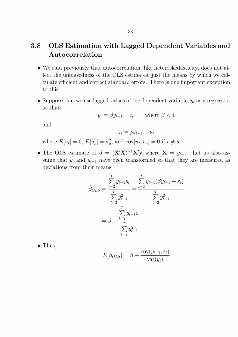
• We said previously that autocorrelation, like heteroskedasticity, does not af-fect the unbiasedness of the OLS estimates, just the means by which we cal-culate efficient and correct standard errors. There is one important exceptionto this.

• Suppose that we use lagged values of the dependent variable, yt as a regressor,so that:

yt = βyt−1 + εt where β < 1

andεt = ρεt−1 + ut

where E[ut] = 0, E[u2t ] = σ2

u, and cov[ut, us] = 0 if t 6= s.

• The OLS estimate of β = (X′X)−1X′y where X = yt−1. Let us also as-sume that yt and yt−1 have been transformed so that they are measured asdeviations from their means.

βOLS =

T∑t=2

yt−1yt

T∑t=2

y2t−1

=

T∑t=2

yt−1(βyt−1 + εt)

T∑t=2

y2t−1

= β +

T∑t=2

yt−1εt

T∑t=2

y2t−1

• Thus,

E[βOLS] = β +cov(yt−1, εt)

var(yt)

34

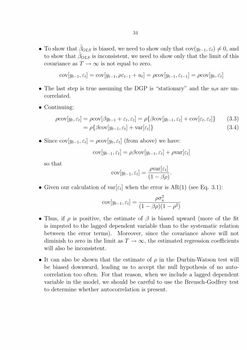
• To show that βOLS is biased, we need to show only that cov(yt−1, εt) 6= 0, andto show that βOLS is inconsistent, we need to show only that the limit of thiscovariance as T →∞ is not equal to zero.

cov[yt−1, εt] = cov[yt−1, ρεt−1 + ut] = ρcov[yt−1, εt−1] = ρcov[yt, εt]

• The last step is true assuming the DGP is “stationary” and the uts are un-correlated.

• Continuing:

ρcov[yt, εt] = ρcov[βyt−1 + εt, εt] = ρβcov[yt−1, εt] + cov[εt, εt] (3.3)

= ρβcov[yt−1, εt] + var[εt] (3.4)

• Since cov[yt−1, εt] = ρcov[yt, εt] (from above) we have:

cov[yt−1, εt] = ρβcov[yt−1, εt] + ρvar[εt]

so that

cov[yt−1, εt] =ρvar[εt]

(1− βρ).

• Given our calculation of var[εt] when the error is AR(1) (see Eq. 3.1):

cov[yt−1, εt] =ρσ2

u

(1− βρ)(1− ρ2)

• Thus, if ρ is positive, the estimate of β is biased upward (more of the fitis imputed to the lagged dependent variable than to the systematic relationbetween the error terms). Moreover, since the covariance above will notdiminish to zero in the limit as T →∞, the estimated regression coefficientswill also be inconsistent.

• It can also be shown that the estimate of ρ in the Durbin-Watson test willbe biased downward, leading us to accept the null hypothesis of no auto-correlation too often. For that reason, when we include a lagged dependentvariable in the model, we should be careful to use the Breusch-Godfrey testto determine whether autocorrelation is present.

35

3.9 Bias and “Contemporaneous Correlation”

• A more immediate question is what general phenomenon produces this biasand how to obtain unbiased estimates when this problem exists. The answerturns out to be a general one, so it is worth exploring.

• The bias (and inconsistency) in this case arose because of a violation of theG-M assumptions E[ε] = 0 and X is a known matrix of constants (“fixed inrepeated samples”). We needed this so that we could say that E[X′ε] = 0.This yielded our proof of unbiasedness.

E[βOLS] = β + E[(X′X)−1X′ε] = β

• Recall we showed that we could relax the assumption that X is fixed inrepeated samples if we substituted the assumption that X is “strictly exoge-nous”, so that E[ε|X] = 0. This will also yield the result that E[X′ε] = 0

• The problem in the case of the lagged dependent variable is that E[X′ε] 6= 0.When there is a large and positive error in the preceding period, we wouldbe likely to get a large and positive εt and a large and positive yt−1.

• Thus, we see a positive relationship between the current error and the regres-sor. This is all that we need to get bias, a “contemporaneous” correlationbetween a regressor and the error term, such that cov[xt, εt] 6= 0.

3.10 Measurement Error

• Another case in which we get biased and inconsistent estimates because ofcontemporaneous correlation between a regressor and the error is measure-ment error.

• Suppose that the true relationship does not contain an intercept and is:

y = βx+ ε

but x is measured with error as z, where z = x + u is what we observe andE[ut] = 0, E[u2

t ] = σ2u.

36

• This implies that x can be written as z − u and the true model can then bewritten as:

y = β(z − u) + ε = βz + (ε− βu) = βz + η

The new disturbance, η, is a function of u (the error in measuring x). z is alsoa function of u. This sets up a non-zero covariance (and correlation) betweenz, our imperfect measure of the true regressor x, and the new disturbanceterm, (ε− βu).

• The covariance between them, as we showed then, is equal to:

cov[z, (ε− βu)] = cov[x+ u, ε− βu] = −βσ2u

• How does this lead to bias? We go back to the original equation for theexpectation of the estimated β coefficient, E[β] = β + (X′X)−1X′ε. It iseasy to show:

E[β] = E[(z′z)−1(z′y)] = E[(z′z)−1(z′(βz + η))] (3.5)

= E[[(x+ u)′(x+ u)]−1(x+ u)′(βx+ ε)] (3.6)

= E

∑i

(x+ u)(βx+ ε)∑i

(x+ u)2

=βx2

x2 + σ2u

= βx2

x2 + σ2u

(3.7)

• Note: establishing a non-zero covariance between the regressor and the errorterm is sufficient to prove bias but is not the same as indicating the directionof the bias. In this special case, however, β is biased downward.

• To show consistency we must show that:

plim β = β +

(X′X

n

)−1(X′ε

n

)= β (recall Q∗ =

(X′X

n

)−1

)

• This involves having to show that plim(

X′εn

)= 0.

• In the case above,

plim β =

plim (1/n)∑i

(x+ u)(βx+ ε)

plim (1/n)∑i

(x+ u)2

=βQ∗

Q∗ + σ2u

37

• Describing the bias and inconsistency in the case of a lagged dependent vari-able with autocorrelation would follow the same procedure. We would lookat the expectation term to show the bias and the probability limit to showinconsistency. See particularly Greene, p. 85.

3.11 Instrumental Variable Estimation

• In any case of contemporaneous correlation between a regressor and the errorterm, we can use an approach known as instrumental variable (or IV) esti-mation. The intuition to this approach is that we will find an instrument forX, where X is the variable correlated with the error term. This instrumentshould ideally be highly correlated with X, but uncorrelated with the errorterm.

• We can use more than one instrument to estimate βIV . Say that we have onevariable, x1, measured with error in the model:

y = β0 + β1x1 + β2x2 + ε

• We believe that there exists a set of variables, Z, that is correlated with x1

but not with ε. We estimate the following model:

x1 = Zα+ u

where the α are the regression coefficients on Z where α = (Z′Z)−1Z′x1.

• We then calculate the fitted or predicted values of x1, or x1, equal to Zα,which is Z(Z′Z)−1Z′x1. These fitted values should not be correlated withthe error term because they are derived from instrumental variables that areuncorrelated with the error term.

• We then use the fitted values x1 in the original model for x1.

y = β0 + β1x1 + β2x2 + ε

This gives an unbiased estimate βIV of β1.

38

In the case of a model with autocorrelation and a lagged dependent variable,Hatanaka (1974), suggests the following IV estimation for the model:

yt = Xβ + γyt−1 + εt

where εt = ρεt−1 + ut

• Use the predicted values from a regression of yt on Xt and Xt−1 as an estimateof yt−1. The coefficient on yt−1 is a consistent estimate of γ, so it can be usedto estimate ρ and perform FGLS.

3.12 In the general case, why is IV estimation unbiased

and consistent?

• Suppose thaty = Xβ + ε

where X contains one regressor that is contemporaneously correlated withthe error term and the other variables are uncorrelated. The intercept andthe variables uncorrelated with the error can serve as their own (perfect)instruments.

• Each instrument is correlated with the variable of interest and uncorrelatedwith the error term. We have at least one instrument for the explanatoryvariable correlated with the error term. By regressing X on Z we get X, thepredicted values of X. For each uncorrelated variable, the predicted value isjust itself since it perfectly predicts itself. For the correlated variables, thepredicted value is the value given by the first-stage model.

X = Zα = Z(Z′Z)−1Z′X

• Then

βIV = (X′X)−1X′y

= [X′Z(Z′Z)−1Z′Z(Z′Z)−1Z′X]−1(X′Z(Z′Z)−1Z′y)

39

• Simplifying and substituting for y we get:

E[βIV ] = E[(X′X)−1X′y]

= E[(X′Z(Z′Z)−1Z′X)−1(X′Z(Z′Z)−1Z′(Xβ + ε)]

= E[X′Z(Z′Z)−1Z′X]−1(X′Z(Z′Z)−1Z′X)β

+ [X′Z(Z′Z)−1Z′X]−1(X′Z(Z′Z)−1Z′ε= β + 0

since E[Z′ε] is zero by assumption.

Section 4

Simultaneous Equations Models and 2SLS

4.1 Simultaneous Equations Models and Bias

• Where we have a system of simultaneous equations we can get biased andinconsistent regression coefficients for the same reason as in the case of mea-surement error (i.e., we introduce a “contemporaneous correlation” betweenat least one of the regressors and the error term).

4.1.1 Motivating Example: Political Violence and Economic Growth

• We are interested in the links between economic growth and political violence.Assume that we have good measures of both.

• We could estimate the following model

Growth = f(V iolence, OtherFactors)

(This is the bread riots are bad for business model).

• We could also estimate a model

V iolence = f(Growth,OtherFactors)

(This is the hunger and privation causes bread riots model).

• We could estimate either by OLS. But what if both are true? Then violencehelps to explain growth and growth helps to explain violence.

• In previous estimations we have treated the variables on the right-hand sideas exogenous. In this case, however, some of them are endogenous becausethey are themselves explained by another causal model. The model now hastwo equations:

Gi = β0 + β1Vi + εi

Vi = α0 + α1Gi + ηi

40

41

4.1.2 Simultaneity Bias

• What happens if we just run OLS on the equation we care about? In general,this is a bad idea (although we will get into the case in which we can). Thereason is simultaneity bias.

• To see the problem, we will go through the following simulation.

1. Suppose some random event sparks political violence (ηi is big). Thiscould be because you did not control for the actions of demagogues instirring up crowds.

2. This causes growth to fall through the effect captured in β1.

3. Thus, Gi and ηi are negatively correlated.

• What happens in this case if we estimate Vi = α0 +α1Gi +ηi by OLS withouttaking the simultaneity into account? We will mis-estimate α1 because growthtends to be low when ηi is high.

• In fact, we are likely to estimate α1 with a negative bias, because E(G′η) isnegative. We may even produce the mistaken result that low growth produceshigh violence solely through the simultaneity.

• To investigate the likely direction and existence of bias, let’s look at E[X′ε]or the covariance between the explanatory variables and the error term.

E[G′η] = E[(β0 + β1V + ε)η] = E[(β0 + β1(α0 + α1G+ η) + ε)η]

• Multiplying through and taking expectations we get:

E[G′η] = E[(β0 + β1α1)′η] + E[β1α1G

′η] + E[β1η′η] + E[ε′η]

• Passing through the expectations operator we get:

E[G′η] = (β0 + β1α1)E[η] + β1α1E[G′η] + β1E[η2] + E[ε]E[η]

(E[ε′η] = E[ε]E[η] because the two error terms are assumed independent).

42

• Since E[ε] = 0 and E[η] = 0 and E[η2] = σ2η, we get:

E[G′η] = β1α1E[G′η] + β1σ2η

So, (1− β1α1)E[G′η] = β1σ2η and E[G′η] =

β1σ2η

(1−β1α1)

• Since this is non-zero, we have a bias in the estimate of α1, the effect ofgrowth, G, on violence, V .

• The equation above indicates that the size of bias will depend on the varianceof the disturbance term, η, and the size of the coefficient on V, β1. Theseparameters jointly determine the magnitude of the feedback effect from errorsin the equation for violence, through the impact of violence, back onto growth.

• The actual computation of the bias term is not quite this simple in the caseof the models above because we will have other variables in the matrix ofright-hand side variables, X.

• Nevertheless, the expression above can help us to deduce the likely directionof bias on the endogenous variable. When we have other variables in themodel, the coefficients on these variables will also be affected by bias, but wecannot tell the direction of this bias a priori.

• How can we estimate the causal effects without bias in the presence of simul-taneity? Doing so will involve re-expressing all the endogenous variables asa function of the exogenous variables and the error terms. This leads to thequestion of the “identification” of the system.

4.2 Identifying the Endogenous Variables

• In order to estimate a system of simultaneous equations (or any equation inthat system) the model must be either “just identified” or “over-identified”.These conditions depend on the exogenous variables in the system of equa-tions.

43

• Suppose we have the following system of simultaneous equations:

Gi = β0 + β1Vi + β2Xi + εi

Vi = α0 + α1Gi + α2Zi + ηi

• We can insert the second equation into the first in order to derive an expres-sion for growth that does not involve the endogenous variable, violence:

Gi = β0 + β1(α0 + α1Gi + α2Zi + ηi) + β2Xi + εi

Then you can pull all the expressions involving Gi onto the left-hand side anddivide through to give:

Gi =β0 + β1α0

(1− β1α1)+

β1α2

(1− β1α1)Zi +

β2

(1− β1α1)Xi +

(εi + β1ηi

1− β1α1

)• We can perform a similar exercise to write the violence equation as:

Vi =α0 + α1β0

(1− α1β1)+

α1β2

(1− α1β1)Xi +

α2

(1− α1β1)Zi +

(ηi + α1εi

1− α1β1

)• We can then estimate these reduced form equations directly.

Gi = γ0 + γ1Zi + γ2Xi + ε∗i

Vi = φ0 + φ1Zi + φ2Xi + η∗i

Where,

γ0 =β0 + β1α0

(1− β1α1)γ1 =

β1α2

(1− β1α1)γ2 =

β2

(1− β1α1)

Also,

φ0 =α0 + α1β0

(1− α1β1)φ1 =

α2

(1− α1β1)φ2 =

α1β2

(1− α1β1)

• In this case, we can we solve backward from this for the original regressioncoefficients of interest, α1 and β1. We can re-express the coefficients from thereduced form equations above to yield:

α1 =φ2

γ2and β1 =

γ1

φ1

44

• This is often labeled “Indirect Least Squares,” a method that is mostly ofpedagogic interest.

• Thus, we uncover and estimate the true relationship between growth andviolence by looking at the relationship between those two variables and theexogenous variables. We say that X and Z identify the model.

• Without the additional variables, there would be no way to estimate α1 andβ1 from the reduced form. The model would be under-identified.

• It is also possible to have situations where there is more than one solutionfor α1 and β1 from the reduced form. This can occur if either equation hasmore than one additional variable.

• Since one way to estimate the coefficients of interest without bias is to es-timate the reduced form and compute the original coefficients from this di-rectly, it is important to determine whether your model is identified. We canestimate just-identified and over-identified models, but not under-identifiedmodels.

4.3 Identification

• There are two conditions to check for identification: the order condition andthe rank condition. In theory, since the rank condition is more binding, onechecks first the order condition and then the rank condition. In practice, veryfew people bother with the rank condition.

4.3.1 The Order Condition

• Let g be the number of endogenous variables in the system (here 2) and letk be the total number of variables (endogenous and exogenous) missing fromthe equation under consideration. Then:

1. If k = g − 1, the equation is exactly identified.

2. If k > g − 1, the equation is over-identified.

3. If k < g − 1, the equation is under-identified.

45

• In general, this means that there must be at least one exogenous variable inthe system, excluded from that equation, in order to estimate the coefficienton the endogenous variable that is included as an explanatory variable in thatequation.

• These conditions are necessary for a given degree of identification. The RankCondition is sufficient for each type of identification. The Rank Conditionassumes the order condition and adds that the reduced form equations musteach have full rank.

4.4 IV Estimation and Two-Stage Least Squares

1. If the model is just-identified, we could regress the endogenous variables onthe exogenous variables and work back from the reduced form coefficients toestimate the structural parameters of interest.

2. If the model is just or over-identified, we can use the exogenous variables asinstruments for Gi and Vi. In this case, we use the instruments to form esti-mates of the two endogenous variables, Gi and Vi that are now uncorrelatedwith the error term and we use these in the original structural equations.

• The second method is generally easier. It is also known as Two-Stage LeastSquares, or 2SLS because it inolves the following stages:

1. Estimate the reduced form equations using OLS. To do this, regress eachendogenous variable on all the exogenous variables in the system. In ourrunning example we would have:

Vi = φ0 + φ1Zi + φ2Xi + η∗i

andGi = γ0 + γ1Zi + γ2Xi + ε∗i

46

2. From these first-stage regressions, estimate Gi and Vi for each observa-tion. The predicted values of the endogenous variables can then be usedto estimate the structural models:

Vi = α0 + α1Gi + α2Zi + ηi

Gi = β0 + β1Vi + β2Xi + εi

• This is just what we would do in standard IV estimation, which is to regressthe problem variable on its instruments and then use the predicted value inthe main regression.

4.4.1 Some Important Observations

• This method gives you unbiased and consistent estimates of α1 and β1. An-other way of saying this is that Gi and Vi are good instruments for Gi andVi.

– A good instrument is highly correlated with the variable that we areinstrumenting for and uncorrelated with the error term. In this case,Gi and Vi are highly correlated with Gi and Vi because we use all theinformation available to us in the exogenous variables to come up withan estimate.

– Second, Gi and Vi are uncorrelated with the error terms ηi and εi becauseof the properties of OLS and the way we estimate the first stage. Aproperty of OLS is that the estimated residuals are uncorrelated withthe regressors and thus uncorrelated with the predicted values (Gi andVi).

– Thus, since the direct effect of growth on Vi, for example, in the firstreduced form equation is part of the estimated residual, the predictedvalue Vi can be treated as exogenous to growth. We have broken thechain of connection that runs from one model to another. We can saythat E[G′η] = 0 and E[V

′ε] = 0.

• When the system is exactly identified, 2SLS will give you results that are iden-tical to those you would obtain from estimated the reduced form equationsand using those coefficients directly to estimate α1 and β1.

47

• There is one case in which estimation of a system of simultaneous equationsby OLS will not give you biased and inconsistent estimates. This is the caseof recursive systems. The following is an example of a recursive system:

yi = α0 + α1Xi + εi

pi = β0 + β1yi + β2Ri + ηi

qi = δ0 + δ1yi + δ2pi + δ3Si + νi

Here, all the errors are independent. In this system of recursive equations,substituting for the endogenous variables yi and pi will ultimately get you tothe exogenous variable Xi, so we don’t get the feedback loops and correlationsbetween regressor and the error that we did in the earlier case.

4.5 Recapitulation of 2SLS and Computation of Goodness-

of-Fit

Let us review the two-stage least square procedure:

1. We first estimated the reduced form equations for Violence and Growth usingOLS.

Vi = φ0 + φ1Zi + φ2Xi + η∗i

andGi = γ0 + γ1Zi + γ2Xi + ε∗i

We used the predicted value of Gi and Vi, or Gi and Vi, as instruments in thesecond stage.

2. We estimated the structural equations using the instruments:

Vi = α0 + α1Gi + α2Zi + ηi

Gi = β0 + β1Vi + β2Xi + εi

And get unbiased coefficients.

• We would normally compute R2 as:

SSR

SST=

∑(xi − x)2β2∑(yi − y)2 or 1− SSE

SST= 1−

∑e2i∑

(yi − y)2 = 1− e′e

y′M0y

48

• In the second stage, however, the estimated residuals are:

ηi = Vi − (α0 + α1Gi + α2Zi)

εi = Gi − (β0 + β1Vi + β2Xi)

• If we use these residuals in our computation of R2 we will get a statistic thattells us how well the model with the instruments fits the data. If we wantan estimate of how well the original structural model fits the data, we shouldestimate the residuals using the true endogenous variables Gi and Vi. Thus,we use:

ηi = Vi − (α0 + α1Gi + α2Zi)

εi = Gi − (β0 + β1Vi + β2Xi)

• This gives us an estimate of the fit of the structural model. There is one oddityin the calculated R2 that may result. When we derived R2, we used the factthat the OLS normal equations estimated residuals such that E[X′e] = 0.This gave us the result that:

SST = SSR + SSE or∑

(yi − y)2 =∑

(xi − x)2β2 +∑

e2i

The variances in y can be completely partitioned between the variance fromthe model and the variance from the residuals. This is no longer the casewhen you re-estimate the errors using the real values of Gi and Vi ratherthan their instruments and you can get cases where SSE > SST. In thiscase, you can get negative values of R2 in the second stage. This may beperfectly okay if the coefficients are of the right sign and the standard errorsare small.

• It also matters in this case whether you estimate R2 as SSRSST or 1− SSE

SST .

4.6 Computation of Standard Errors in 2SLS

• Let us denote all the original right-hand side variables in the two structuralmodels as X, the instrumented variables as X, and the exogenous variablesthat we used to estimate X as Z.

49

• In section 3.12, we showed that:

βIV = (X′X)−1X′y = (X′Z(Z′Z)−1Z′X)−1(X′Z(Z′Z)−1Z′(Xβ + ε)

= β + (X′Z(Z′Z)−1Z′X)−1(X′Z(Z′Z)−1Z′ε)

= β + (X′X)−1(X′ε)

var[βIV ] = E[(βIV − β)(βIV − β)′] = E[(X′X)−1X′εε′X(X′X)−1]

• If the errors conform to the Gauss-Markov assumptions then, E[εε′] = σ2IN

andvar[βIV ] = σ2(X′X)−1

• To estimate σ2 we would normally use e′e(n−K) .

• As with R2, we should use the estimated residuals from the structural modelwith the true variables in it rather than the predicted values. These areconsistent estimates of the true disturbances.

ηi = Vi − (α0 + α1Gi + α2Zi)

εi = Gi − (β0 + β1Vi + β2Xi)

• The IV estimator can have very large standard errors, because the instru-ments by which X is proxied are not perfectly correlated with it and yourresiduals will be larger.

50

4.7 Three-Stage Least Squares

• What if, in the process above, we became concerned that E[εε′] 6= σ2IN?

• We would perform three-stage least squares.

1. Estimate the reduced form equations in OLS and calculate predictedvalues of the endogenous variables Gi and Vi.

2. Estimate the structural equations with the fitted values.

3. Use the residuals calculated in the manner above (using the actual val-ues of Gi and Vi) to test for heteroskedasticity and/or autocorrelationand compute the appropriate standard errors if either are present. Inthe case of heteroskedasticity, this would mean either FGLS and a datatransformation or White-Corrected Standard Errors. In the case of auto-correlation, this would mean either FGLS and a data transformation orNewey-West standard errors.

51

4.8 Different Methods to Detect and Test for Endogeneity

1. A priori tests for endogeneity – Granger Causality.

2. A test to look at whether the coefficients under OLS are markedly differentfrom the coefficients under 2SLS – Hausman Specification Test.

4.8.1 Granger Causality

• A concept that is often used in time series work to define endogeneity is“Granger Causality.” What it defines is really “pre-determinedness.” Grangercausality is absent when we can say that:

f(xt|xt−1, yt−1) = f(xt|xt−1)

The definition states that in the conditional distribution, lagged values of yt

add no information to our prediction of xt beyond that provided by laggedvalues of xt itself.

• This is tested by estimating:

xt = β0 + β1xt−1 + β2yt−1 + εt

• If a t-test indicates that β2 = 0, then we say that y does not Granger cause x.If y does not Granger cause x, then x is often said to be exogenous in a systemof equations with y. Here, exogeneity implies only that prior movements iny do not lead to later movements in x.

• Kennedy has a critique of Granger Causality in which he points out that underthis definition weather reports “cause” the weather and that an increase inChristmas card sales “cause” Christmas. The problem here is that variablesthat are based on expectations (that the weather will be rainy, that Christmaswill arrive) cause earlier changes in behavior (warnings to carry an umbrellaand a desire to buy cards).

52

4.8.2 The Hausman Specification Test

• If βOLS and βIV are “close” in magnitude, then it would appear that endo-geneity is not producing bias.

• This intuition has been formalized into a test by the econometrician JerryHausman. The test is called a specification test because it tells you whetheryou were right to use 2SLS. In this case, however, it can also be used to testthe original assumption of endogeneity. The logic is as follows:

• H0: There is no endogeneity

In this case both βOLS and βIV are consistent and βOLS is efficient relativeto βIV (recall that OLS is BLUE).

• H1: There is endogeneity

In this case βIV remains consistent while βOLS is inconsistent. Thus, theirvalues will diverge.

• The suggestion, then, is to examine d = (βIV − βOLS). The question is howlarge this difference should be before we assume that something is up. Thiswill depend on the variance of d.

• Thus, we can form a Wald statistic to test the hypothesis above:

W = d′[Estimated Asymptotic Variance(d)]−1d

• The trouble, for a long time, was that no-one knew how to estimate this vari-ance since it should involve the covariances between βIV and βOLS. Hausmansolved this by proving that the covariance between an efficient estimator βOLS

of a parameter vector β and its difference from an inefficient estimator βIV

of the same parameter vector is zero (under the null). (For more details seeGreene Section 5.5.)

• Based on this proof, we can say that:

Asy. var[βIV − βOLS] = Asy. var[βIV ]− Asy. var[βOLS]

53

• Under the null hypothesis, we are using two different but consistent estimatorsof σ2. If we use s2 as a common estimator of this, the Hausman statistic willbe:

H =(βIV − βOLS)′[(X′X)−1 − (X′X)−1]−1(βIV − βOLS)

s2

• This test statistic is distributed χ2 but the appropriate degrees of freedom forthe test statistic will depend on the context (i.e., how many of the variablesin the regression are thought to be endogenous).

4.8.3 Regression Version

• The test statistic above can be automatically computed in most standardsoftware packages. In the case of IV estimation (of which 2SLS is an example)there is a completely equivalent way of running the Hausman test using an“auxiliary regression”.

• Assume that the model has K1 potentially endogenous variables, X, and K2

remaining variables, W. We have predicted values of X, X, based on thereduced form equations. We estimate the model:

y = Xβ + Xα+ Wγ + ε

• The test for endogeneity is performed as an F -test on the K1 regressioncoefficients α being different from zero, where the degrees of freedom are K1

and (n− (K1 +K2)−K1). If α = 0, then X is said to be exogenous.

• The intuition is as follows. If the X variables are truly exogenous, then theβ should be unbiased and there will be no extra information added by thefitted values. If the X variables are endogenous, then the fitted values willadd extra information and account for some of the variation in y. Thus, theywill have a coefficient on them significantly different from zero.

• Greene does not go through the algebra to prove that the augmented regres-sion is equivalent to running the Hausman test but refers readers to Davidsonand MacKinnon (1993). Kennedy has a nice exposition of the logic above onp. 197–198.

54

4.8.4 How to do this in Stata

1. 2SLS or To perform any type of IV estimation, see ivreg.

The command is:

ivreg (depvar) [varlist1] [varlist2=varlist IV]

2. To perform 3SLS, see reg3

3. To perform a Hausman test, see hausman

The hausman test is used in conjunction with other regression commands.To use it, you would:

Run the less efficient model (here IV or reg3)

hausman, save

Run the fully efficient model (here OLS)

hausman

4.9 Testing for the Validity of Instruments

• We stated previously that the important features of “good” instruments, Z,are that they be highly correlated with the endogenous variables, X, anduncorrelated with the true errors, ε.

• The first requirement can be tested fairly simply by inspecting the reducedform model in which each endogenous variables is regressed on its instrumentsto yield predicted values, X. In a model with one instrument, look at thet-statistic. In an IV model with multiple instruments, look at the F -statistic.

• For the second requirement, the conclusion that Z and ε are uncorrelated inthe case of one instrument must be a leap of faith, since we cannot observe εand must appeal to theory or introspection.

55

• For multiple instruments, however, so long as we are prepared to believe thatone of the instruments is uncorrelated with the error, we can test the assump-tion that remaining instruments are uncorrelated with the error term. Thisis done via an auxiliary regression and is know as “testing over-identificationrestrictions.”

• It is called this because, if there is more than one instrument, then the en-dogenous regressor is over-identified. The logic of the test is simple.

– If at least one of the instruments is uncorrelated with the true error term,then 2SLS gives consistent estimates of the true errors.

– The residuals from the 2SLS estimation can then be used as the depen-dent variable in a regression on all the instruments.

– If the instruments are, in fact, correlated with the true errors, then thiswill be apparent in a significant F -statistic on the instruments beingjointly significant for the residuals.

• Thus, the steps in the test for over-identifying restrictions are as follows:

1. Estimate the 2SLS residuals using ηi = Vi − α0 + α1Gi + α2Zi. Use ηi asyour consistent estimate of the true errors.

2. Regress ηi on all the instruments used in estimating the 2SLS coefficients.

3. You can approximately test the over-identifying restrictions via inspec-tion of the F -statistic for the null hypothesis that all instruments arejointly insignificant. However, since the residuals are only consistent forthe true errors, this test is only valid asymptotically and you shouldtechnically use a large-sample test.

– An alternative is to use n ·R2 a∼ χ2 w/ df = # of instruments − # ofendogenous regressors. If reject the null ⇒ at least some of the IVsare not exogenous.

Section 5

Time Series Modeling

5.1 Historical Background

• Genesis of modern time series models: large structural models of the macro-economy, which involved numerous different variables, were poor predictorsof actual economic outcomes.

• Box and Jenkins showed that the present and future values of an economicvariable could often be better predicted by its own past values than by othervariables—dynamic models.

• In political science: used in models of presidential approval and partisanidentity.

5.2 The Auto-Regressive and Moving Average Specifica-

tions

• A time series is a sequence of numerical data in which each observation isassociated with a particular instant in time.

• Univariate time series analysis: analysis of a single sequence of data

• Multivariate time series analysis: several sets of data for the same sequenceof time periods

• The purpose of time series analysis is to study the dynamics, or temporalstructure of the data.

• Two representations of the temporal structure that will allow us to describealmost all dynamics (for “stationary” sequences) are the auto-regressive andmoving-average representations.

56

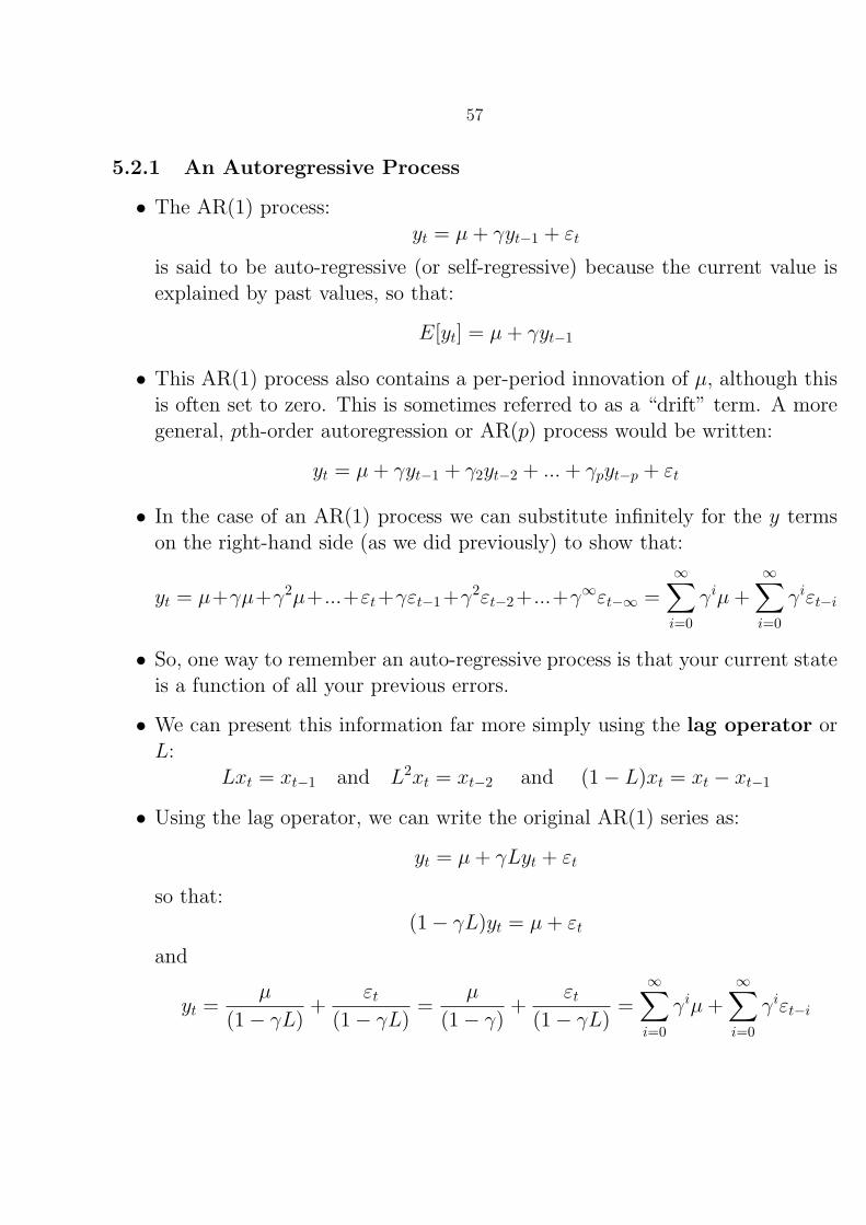
57

5.2.1 An Autoregressive Process

• The AR(1) process:yt = µ+ γyt−1 + εt

is said to be auto-regressive (or self-regressive) because the current value isexplained by past values, so that:

E[yt] = µ+ γyt−1

• This AR(1) process also contains a per-period innovation of µ, although thisis often set to zero. This is sometimes referred to as a “drift” term. A moregeneral, pth-order autoregression or AR(p) process would be written:

yt = µ+ γyt−1 + γ2yt−2 + ...+ γpyt−p + εt

• In the case of an AR(1) process we can substitute infinitely for the y termson the right-hand side (as we did previously) to show that:

yt = µ+γµ+γ2µ+...+εt+γεt−1+γ2εt−2+...+γ

∞εt−∞ =∞∑i=0

γiµ+∞∑i=0

γiεt−i

• So, one way to remember an auto-regressive process is that your current stateis a function of all your previous errors.

• We can present this information far more simply using the lag operator orL:

Lxt = xt−1 and L2xt = xt−2 and (1− L)xt = xt − xt−1

• Using the lag operator, we can write the original AR(1) series as:

yt = µ+ γLyt + εt

so that:(1− γL)yt = µ+ εt

and

yt =µ

(1− γL)+

εt

(1− γL)=

µ

(1− γ)+

εt

(1− γL)=

∞∑i=0

γiµ+∞∑i=0

γiεt−i

58

• The last step comes from something we encountered before: how to representan infinite series:

A = x(1 + a+ a2 + ...+ an)

If |a| < 1, then the solution to this series is approximately A = x(1−a) . In

other words, the sequence is convergent (has a finite solution).

• Thus, for the series∞∑i=0

γiεt−i = εt+γεt−1+γ2εt−2+... = εt+γLεt+γ

2L2εt+...

we have that, a = γL and∞∑i=0

γiεt−i = εt

(1−γL) .

• For similar reasons,∞∑i=0

γiµ = µ(1−γL) = µ

(1−γ) because Lµ = µ In other words,

µ, the per-period innovation is not subscripted by time and is assumed to bethe same in each period.

5.3 Stationarity

• So, an AR(1) process can be written quite simply as:

yt =µ

(1− γ)+

εt

(1− γL)

• Recall, though, that this requires that |γ| < 1. If |γ| ≥ 1 then we cannoteven define yt. yt keeps on growing as the error terms collect. Its expectationwill be undefined and its variance will be infinite.

• That means that we cannot use standard statistical procedures if the auto-regressive process is characterized by |γ| > 1. This is known as the station-arity condition and the data series is said to be stationary if |γ| < 1.

• The problem is that our standard results for consistency and for hypothesistesting requires that (X′X)−1 is a finite, positive matrix. This is no longertrue. The matrix (X′X) will be infinite when the data series X is non-stationary.

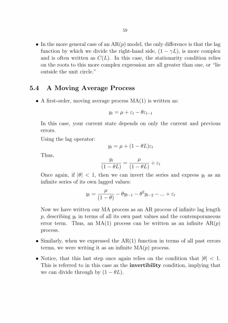
59

• In the more general case of an AR(p) model, the only difference is that the lagfunction by which we divide the right-hand side, (1 − γL), is more complexand is often written as C(L). In this case, the stationarity condition relieson the roots to this more complex expression are all greater than one, or “lieoutside the unit circle.”

5.4 A Moving Average Process

• A first-order, moving average process MA(1) is written as:

yt = µ+ εt − θεt−1

In this case, your current state depends on only the current and previouserrors.

Using the lag operator:yt = µ+ (1− θL)εt

Thus,yt

(1− θL)=

µ

(1− θL)+ εt

Once again, if |θ| < 1, then we can invert the series and express yt as aninfinite series of its own lagged values:

yt =µ

(1− θ)− θyt−1 − θ2yt−2 − ...+ εt

Now we have written our MA process as an AR process of infinite lag lengthp, describing yt in terms of all its own past values and the contemporaneouserror term. Thus, an MA(1) process can be written as an infinite AR(p)process.

• Similarly, when we expressed the AR(1) function in terms of all past errorsterms, we were writing it as an infinite MA(p) process.

• Notice, that this last step once again relies on the condition that |θ| < 1.This is referred to in this case as the invertibility condition, implying thatwe can divide through by (1− θL).

60

• If we had a more general, MA(q) process, with more lags, we could go throughthe same steps, but we would have a more complex function of the lags than(1− θL). Greene’s textbook refers to this function as D(L). In this case, theinvertibility condition is satisfied when the roots of D(L) lie outside the unitcircle (see Greene, 5th Ed., pp. 611–615).

5.5 ARMA Processes

• Time series can also be posited to contain both AR and MA terms. However,if we go through the inversion above, getting:

yt =µ

(1− θ)− θyt−1 − θ2yt−2 − ...+ εt

and then substitute for the lagged yts in the AR process, we will arrive at anexpression for yt that is based only on a constant and a complex function ofpast errors. See Greene p. 611 (Fifth Edition) for an example.

• We could also write an ARMA(1,1) process as:

yt =µ

(1− γ)+

(1− θL)

(1− γL)εt

• An ARMA process with p autoregressive components and q moving averagecomponents is called an ARMA(p, q) process.

• Where does this get us? We can estimate yt and apply the standard proofsof consistency if the time series is stationary, so it makes sense to discusswhat stationarity means in the context of time series data. If the time seriesis stationary and can be characterized by an AR process, then the modelcan be estimated using OLS. If it is stationary and characterized by an MAprocess, you will need to use a more complicated estimation procedure (non-linear least squares).

61

5.6 More on Stationarity

• There are two main concepts of stationarity applied in the literature.

1. Strict Stationarity: For the process yt = ρyt−1 + εt, strict stationarityimplies that:

– E[yt] = µ exists and is independent of t.

– var[yt] = γ0 is a finite, positive constant, independent of t.

– cov[yt, ys] = γ(|t− s|) is a finite function of |t− s|, but not of t or s.

– AND all other “higher order moments” (such as skewness or kurtosis)are also independent of t.

2. Weak Stationarity (or covariance stationarity): removes the conditionon the “higher order moments” of yt.

• A stationary time series will tend to revert to its mean (mean reversion) andfluctuations around this mean will have a broadly consistent amplitude.

• Intuition: if we take two slices from the data series, they should have approxi-mately the same mean and the covariance between points should depend onlyon the number of time periods that divide them. This will not be true of “in-tegrated” series, so we will have to transform the data to make it stationarybefore estimating the model.

5.7 Integrated Processes, Spurious Correlations, and Test-

ing for Unit Roots

• One of the main concerns w/ non-stationary series is spurious correlation.

• Suppose you have a non-stationary, highly trending series, yt, and you regressit on another highly trending series, xt. You are likely to find a significantrelationship between yt and xt even when there was none, because we seeupward movement in both produced in their own dynamics.

• Thus, when the two time series are non-stationary, standard critical valuesof the t and F statistics are likely to be highly misleading about true causalrelationships (see Greene p. 778).

62

• The question is, what kind of non-stationary sequence do we have and howcan we tell it’s non-stationary. Consider the following types of non-stationaryseries:

1. The Pure Random Walk

yt = yt−1 + εt

This DGP can also be written as:

yt = y0 +∑

εt

E[yt] = E[y0 +∑

εt] = y0

– In similar fashion it can be shown that the variance of yt = tσ2.Thus, the mean is constant but the variance increases indefinitely asthe number of time points grows.

– If you take the first difference of the data process, however, ∆yt =yt − yt−1, we get:

yt − yt−1 = εt

The mean of this process is constant (and equal to zero) and itsvariance is also a finite constant. Thus, the first difference of a randomwalk process is a difference stationary process.

2. The Random Walk with Drift

yt = µ+ yt−1 + εt

For the random walk with drift process, we can show that E[yt] = y0 + tµ

and var[yt] = tσ2. Both the mean and the variance are non-constant.

– In this case, first differencing of the series also will give you a variablethat has a constant mean and variance.

63

3. The Trend Stationary Process

yt = µ+ βt+ εt

– yt is non-stationary because the mean of yt is equal to µ+ βt, whichis non-constant, although its variance is constant and equal to σ2.

– Once the values of µ and β are known, however, the mean can beperfectly predicted. Therefore, if we subtract the mean of yt fromyt, the resulting series will be stationary, and is thus called a trendstationary process in comparison to the difference stationary processesdescribed above.

• Each of these series is characterized by a unit root, meaning that the coefficienton the lagged value of yt = 1 in each process. For a trend stationary process,this follows because you can re-write the time series as yt = µ + βt + εt =yt−1 + β + εt − εt−1.

• In each case, the DGP can be written as:

(1− L)yt = α+ ν

where α = 0, µ, and β respectively in each process and ν is a stationaryprocess.

• In all cases, the data should be detrended or differenced to produce a station-ary series. But which? The matter is not of merely academic interest, sincedetrending a random walk will induce autocorrelation in the error terms ofan MA(1) type.

64

• A unit-root test (described in Greene, p. 637) is based on a model that neststhe different processes above into one regression that you run to test theproperties of the underlying data series:

yt = µ+ βt+ γyt−1 + εt

• Next subtract yt−1 from both sides of the equation to produce the equationbelow. This produces a regression with a (difference) stationary dependentvariable (even under the null of non-stationarity) and this regression formsthe basis for Dickey-Fuller tests of a unit root:

yt − yt−1 = µ+ βt+ (γ − 1)yt−1 + εt

– A test of the hypothesis that (γ − 1) is zero gives evidence for a randomwalk, because this ⇒ γ = 1.

– If (γ − 1) = 0 and µ is significantly different from zero we have evidencefor a random walk with drift.

– If (γ − 1) is significantly different from zero (and < 0) we have evidenceof a stationary process.

– If (γ − 1) is significantly different from and less than zero, and β (thecoefficient on the trend variable) is significant, we have evidence for atrend stationary process.

• There is one complication. Two statisticians, Dickey and Fuller (1979, 1981)showed that if the unit root is exactly equal to one, the standard errors willbe under-estimated, so that revised critical values are required for the teststatistic above.

• For this reason, the test for stationarity is referred to as the Dickey-Fullertest. The augmented Dickey-Fuller test applies to the same equation abovebut adds lags of the first difference in y, (yt − yt−1).

• One problem with the Dickey-Fuller unit-root test is that it has low powerand seems to privilege the null hypothesis of a random walk process over thealternatives.

65

• To sum up: If your data looks like a random walk, you will have to difference ituntil you get something that looks stationary. If your data looks like it’s trendstationary, you will have to de-trend it until you get something stationary.An ARMA model carried out on differenced data is called an ARIMA model,standing for “Auto-Regressive, Integrated, Moving-Average.”

5.7.1 Determining the Specification

• You have data that is now stationary. How do you figure out which ARMAspecification to use? How many, if any, AR terms should there be? Howmany, if any, MA terms?

• As a means of deciding the specification, analysts in the past have looked atthe autocorrelations and partial autocorrelations between yt and yt−s. This isalso known as looking at the autocorrelation function (ACF) and the partialautocorrelation function (or PACF).

• Recall that

corr(εt, εt−s) =cov(εt, εt−s)√

var(εt)√

var(εt−s)=E[εtεt−s]

E[ε2t

] =γs

γ0

• If yt and yt−s are both expressed in terms of deviations from their means, andif var(yt) = var(yt−s) then:

corr(yt, yt−s) =cov(yt, yt−s)√

var(yt)√

var(yt−s)=E[ytyt−s]

E[y2t ]

=γs

γ0

5.8 The Autocorrelation Function for AR(1) and MA(1)

processes

• We showed in the section on autocorrelation in the error terms that if yt =ρyt−1 + εt then corr[yt, yt−s] = ρs.

• In this context, εt is white noise. E[εt] = 0, E[ε2t ] = σ2

ε , E[εtεt−1] = 0

• Thus, the autocorrelations for an AR(1) process tend to die away gradually.

66

• By contrast, the autocorrelations for an MA(1) process die away abruptly.

• Letyt = εt − θεt−1

Then

γ0 = var[yt] = Eyt−E[yt]2 = E[(εt−θεt−1)2] = E(ε2

t )+θ2E(ε2

t−1) = (1+θ2)σ2ε

and

γ1 = cov[yt, yt−1] = E[(εt − θεt−1)(εt−1 − θεt−2)] = −θE[ε2t−1] = −θσ2

ε

• The covariances between yt and yt−s when s > 1 are zero, because the ex-pression for yt only involves two error terms. Thus, the ACF for an MA(1)process has one or two spikes and then shows no autocorrelation.

5.9 The Partial Autocorrelation Function for AR(1) and

MA(1) processes

• The partial autocorrelation is the simple correlation between yt and yt−s minusthat part explained by the intervening lags.

• Thus, the partial autocorrelation between yt and yt−s is estimated by the lastcoefficient in the regression of yt on [yt−1, yt−2, ..., yt−s]. The appearance of thepartial autocorrelation function is the reverse of that for the autocorrelationfunction. For a true AR(1) process,

yt = ρyt−1 + εt

• There will be an initial spike at the first lag (where the autocorrelation equalsρ) and then nothing, because no other lagged value of y is significant.

• For the MA(1) process, the partial autocorrelation function will look like agradually declining wave, because any MA(1) process can be written as aninfinite AR process with declining weights on the lagged values of y.

67

5.10 Different Specifications for Time Series Analysis

• We now turn to models in which yt is related to its own past values and a setof exogenous, explanatory variables, xt.

• The pathbreaking time series work in pol. sci. concerned how presidentialapproval levels respond to past levels of approval and measures of presidentialperformance. Let’s use At, standing for the current level of approval, as thedependent variable for our examples here.

– More on this topic can be found in an article by Neal Beck, 1991, “Com-paring Dynamic Specifications,” Political Analysis.

1. The Static ModelAt = βXt + εt

Comment from Beck, “This assumes that approval adjusts instantaneouslyto new information (“no stickiness”) and that prior information is of noconsequence (“no memory”).

2. The Finite Distributed Lag Model

At =M∑i=0

βiXt−i + εt

This allows for memory but may have a large number of coefficients,reducing your degrees of freedom.

3. The Exponential Distributed Lag (EDL) Model

At =M∑i=0

(Xt−iλi)β + εt

Reduces the number of parameters that you now have to estimate. Inthe case in which T can be taken as infinite, this can also be written as:

At =∞∑i=0

Xtβ(λL)i + εt =Xtβ

(1− λL)+ εt

68

4. The Partial Adjustment ModelMultiply both sides of the EDL model above by the “Koyck Transforma-tion” or (1− λL). After simplification, this will yield:

At = Xtβ + λAt−1 + εt − λεt−1

– This says that current approval is a function of current exogenousvariables and the past value of approval, allowing for memory andstickiness. By including a lagged dependent variable, you are actu-ally allowing for all past values of X to affect your current level ofapproval, with more recent values of X weighted more heavily.

– If the errors in the original EDL model were also AR(1), that isto say if errors in preceding periods also had an effect on currentapproval (e.g., ut = λut−1 + εt), with the size of that effect falling inan exponential way, then the Koyck transformation will actually giveyou a specification in which the errors are iid. In other words:

At = Xtβ + λAt−1 + εt

This specification is very often used in applied work with a stationaryvariable whose current level is affected by memory and stickiness. Ifthe error is indeed iid, then the model can be estimated using OLS.

5. Models for “Difference Stationary” Data: The Error CorrectionModelOften, if you run an augmented Dickey-Fuller test and are unable toreject the hypothesis that your data has a unit root, you will wind uprunning the following type of regression:

∆At = ∆Xtβ + εt

As Beck notes (p. 67) this is equivalent to saying that only the infor-mation in the current period counts and that it creates an instantaneouschange in approval. This can be restrictive.

– Moreover, it will frequently result in finding no significant results infirst differences, although you have strong theoretical priors that thedependent variable is related to the independent variables.

69

– What you can do in this instance, with some justification, is to run anError Correction Model that allows you to estimate both long-termand short-term dynamics.

– Let us assume, for the moment, that both A and X are integrated (oforder one). Then we would not be advised to include them in a modelin terms of levels. However, if they are in a long-term, equilibriumrelationship with one another, then the errors

et = At −Xtα

should be stationary. Moreover, if we can posit that people respondto their “errors” and that gradually the relationship comes back intoequilibrium, then we can introduce the error term into a model of thechange in approval. This is the Error Correction Model.

∆At = ∆Xtβ + γ(At−1 −Xt−1α) + εt

The γ coefficient in this model is telling you how fast errors are ad-justed. An attraction of this model is that it allows you to estimatelong-term dynamics (in levels) and short-term dynamics (in changes)simultaneously.

5.11 Determining the Number of Lags

• In order to select the appropriate number of lags of the dependent variable(in an AR(p)) model, you could use the “general to specific” methodology.Include a number of lags that you think is more than sufficient and take outof the model any lags that are not significant.

• Second, analysts are increasingly using adjusted measures of fit (analogousto R2) that compensate for the fact that as you include more lags (to fit thedata better) you are reducing the degrees of freedom.

• The two best known are the Akaike Information Criterion and the SchwartzCriterion. Both are based on the standard error of the estimate (actuallyon s2). Thus, you want to minimize both, but you are penalized when youinclude additional lags to reduce the standard error of the estimate.

70

• The equations for the two criteria are:

AIC(K) = ln

(e′e

n

)+

2K

n

SC(K) = ln

(e′e

n

)+K lnn

n

The Schwartz Criterion penalizes degrees of freedom lost more heavily.

• The model with the smallest AIC or SC indicates the appropriate numberof lags.

5.12 Determining the Correct Specification for your Er-

rors

• Beck gives examples (p. 60 and p. 64) where the error term is autocorrelatedeven when you have built in lags of the dependent variable.

• This could occur if the effect of past errors dies out at a different rate thandoes the effect of past levels in the explanatory variables. If this is the case,you could still get an error term that is AR or MA, even when you haveintroduced a lagged dependent variable, although doing this will generallyreduce the autocorrelation.

• The autocorrelation could be produced by an AR or an MA process in theerror term. To determine which, you might again look at the autocorrelationsand partial autocorrelations.

• We know how to transform the data in the case where the errors are AR(1)using the Cochrane-Orcutt transformation or using Newey-West standard er-rors. If the model was otherwise static, I would also suggest these approaches.

71

5.13 Stata Commands

• Dickey-Fuller Tests:

dfuller varname, noconstant lags(#) trend regress

• The Autocorrelation and Partial Autocorrelation Function:

corrgram varname, lags(#)

ac varname, lags(#)

pac varname, lags(#)

• ARIMA Estimation:

arima depvar [varlist], ar(numlist) ma(numlist)

72

Part II

Maximum Likelihood Estimation

Section 6

Intro to Maximum LikelihoodOur basic task: make inferences about the relationship between variables in apopulation based on what’s going on in a sample

Fundamentals:

• Assume distribution for data—i.e., all observations are drawn from the samedistribution.

• Given distribution we can write down a function that describes how thedata for an individual were generated.

• Key assumption: observations in sample are independent and identicallydistributed (iid)—we get independence by assuming we have a randomsample.

– If observations are independent, then the joint density of theobservations is just the product of their marginal densities:

f(x1, x2, . . . , xn−1, xn) = f(x1) · f(x2) · · · f(xn−1) · f(xn)

– This product gives the likelihood of the sample.

• ML means we choose the parameters that maximize the likelihood ofobserving the sample that we actually observe.

• This requires that we find the maximum of the likelihood function w.r.t. tothe parameters of interest.

73

74

To fix ideas consider the following example:

• Flipping coins (Bernoulli trials):

Y =

1 for a head0 for a tail

• Let p = Pr(Y = 1)

• Flip coin n times to obtain the sample: Y1, . . . , Yn.

• Key assumption: coin flips are independent and prob of observing a head ora tail is the same at each trial.

• From the given sample, we want to estimate p.

• Note that p is population mean:

E(Yi) = Pr(Yi = 1) · 1 + Pr(Yi = 0) · 0= Pr(Yi = 1)

= p

• To estimate the population mean we typically use the sample mean:

Y =∑n

i=1 Yi

n .

• Note that the proportion of heads is given by p =∑n

i=1 Yi

n .

75

• Let Li = likelihood for observation i.

• What is likelihood for ith toss?

• For each observation could get a head which happens with prob p or couldget a tail which happens with prob 1− p:

Li = pYi · (1− p)(1−Yi) (6.1)

• If we have iid sampling then

L =[pY1 · (1− p)(1−Y1)

] [pY2 · (1− p)(1−Y2)

]· · ·[pYn · (1− p)(1−Yn)

]= Πn

i=1pYi · (1− p)(1−Yi).

• Usually take logs because they are easier to deal with (Remember:ln ab = b ln a and ln(a · b) = ln a+ ln b):

lnL =n∑

i=1

lnLi

=n∑

i=1

ln[pYi(1− p)(1−Yi)

]=

n∑i=1

[Yi ln p+ (1− Yi) ln(1− p)]

76

• Want to choose value for p than maximizes lnL. How do we do this?

• Some calculus:

– To find the maximum of a function with respect to some parameter, wetake the derivative of the function with respect to that parameter andthen set result equal to zero and solve for the parameter.

– To make sure it’s a maximum we then check to make sure the secondderivative is negative.

• For example, consider the function f(x) = −x2 + 2x.

df(x)

dx= −2x+ 2

• Setting this equal to zero and solving for x gives x = 1.

• Checking the second derivative:

d2f(x)

d2x=d(−2x+ 2)

dx= −2

which implies we have a maximum rather than a minimum.

77

• Returning to our likelihood function:

d lnL

dp=

n∑i=1

[Yi

1

p− (1− Yi)

1

1− p

]since

d ln a

da=

1

a

(Note: must also use the chain rule).

• Setting the derivative equal to zero and solving gives:

n∑i=1

[Yi

1

p− (1− Yi)

1

1− p

]= 0∑n

i=1 [Yi(1− p)− (1− Yi)p]

p(1− p)= 0

n∑i=1

[Yi − pYi − p+ pYi] = 0

np =n∑

i=1

Yi

p =

∑ni=1 Yi

n

• Checking the second derivative of lnL w.r.t. p we find that it is alwaysnegative:

d2 lnL

d2p= −

n∑i=1

Yi1

p2 −n∑

i=1

(1− Yi)1

(1− p)2

so p =∑n

i=1 Yi

n yields a global max. of the log likelihood function.

Section 7

Maximum Likelihood In Depth• Suppose we have random sample of n observations where each observations

has the density f(xi, θ). Then the joint pdf is given by

f(x1, . . . , xn, θ) = f(x1, θ) · · · f(xn, θ)

= Πni=1f(xi, θ)

= L(θ)

(7.1)

• We usually deal with the log of the likelihood function:

lnL(θ) =n∑

i=1

ln f(xi, θ)

• The MLEs of θ, denoted θ, are the values of the parameters that maximizeL(θ).

• Note that θ also maximizes lnL(θ) because ln is a monotonic function.

• The necessary condition for maximizing lnL(θ) is

∂ lnL(θ)

∂θ= 0

78

79

• Suppose we have a sample from a normal distribution with mean µ andvariance σ2. Then the likelihood function is

L(µ, σ2) = Πni=1

1√2πσ2

exp

(−1

2

(xi − µ)2

σ2

)= Πn

i=1(2πσ2)−1/2e−(1/(2σ2))(xi−µ)2

= (2πσ2)−n/2e−(1/(2σ2))∑n

i=1(xi−µ)2

(7.2)

• Taking the log gives

lnL(µ, σ2) = −n2

ln(2π)− n

2lnσ2 − 1

2σ2

n∑i=1

(xi − µ)2

• Taking first derivatives gives

∂ lnL

∂µ=

1

σ2

∑i

(xi − µ) (7.3)

∂ lnL

∂σ2 = − n

2σ2 +1

2σ4

∑i

(xi − µ)2 (7.4)

• Setting (7.3) equal to zero and solving for µ, gives the MLE µ:

µ =1

n

∑i

xi = x

80

• To find the variance of the MLE, we need to take the second derivativew.r.t. the parameter of interest.

– The variance-covariance matrix is a function of the Hessian—thematrix of second derivatives.

– Specifically it is the inverse of the negative of the expectation of thesecond derivatives.

• From our example,

var(µ) =

[−E

(∂2 lnL

∂µ2

)]−1

=σ2

n

• Setting (7.4) equal to zero, inserting µ for µ and solving for σ2 gives theMLE:

σ2 =1

n

∑i

(xi − x)2

• Note that the unbiased estimator for σ2 is

σ2 =1

n− 1

∑i

(xi − x)2

• The attractiveness of MLEs stems from their large sample or asymptoticproperties.

81

7.1 Asymptotic Properties of MLEs

1. The MLE is consistent.

That is,limn→∞ Pr(|θ − θ| > ε) = 0

where ε is some small positive number. Or simply

plim θ = θ

2. The MLE is asymptotically normally distributed:

θa∼ N

[θ, I(θ)−1]

where I(θ) is the information matrix. The information matrix containsthe negatives of the expected values of the second derivatives.

[I(θ)]−1 =

−E

[∂2 lnL(θ)

∂θ∂θ′

]−1

=

E

[(∂ lnL(θ)

∂θ

)(∂ lnL(θ)

∂θ′

)]−1

82

3. The MLE is asymptotically efficient and achieves the Cramer-Rao lowerbound for consistent estimators:

Asy. var[θ] = [I(θ)]−1

• The Cramer-Rao inequality states that, given certain regularityconditions, if θ is an unbiased estimator of θ then

var(θ) ≥ 1

−E[

∂2 lnL∂θ2

]• The Cramer-Rao lower bound gives the lower bound for the variance of

unbiased estimators.

• Since the MLE achieves this lower bound, we know that the MLE hasthe minimum variance acheivable by a consistent estimator.

83

• Example: Consider L(µ, σ2), the likelihood function in equation 7.2.Taking the second derivatives gives

∂2 lnL

∂µ2 = − n

σ2

∂2 lnL

∂(σ2)2 =n

2σ4 −1

σ6

∑i

(xi − µ)2

∂2 lnL

∂µ∂σ2 = − 1

σ4

∑i

(xi − µ)

so the information matrix is

I(µ, σ2) =

[nσ2 00 n

2σ4

]

• Another important property of the MLE is invariance: if θ is the MLE ofθ and if g(θ) is a continuous function, then the MLE of g(θ) is g(θ).

• Note that the Asy. var[θ] is a function of the unknown parameters θ, so wehave to come up with an estimator for it. Two consistent estimators are

Asy. var[θ] =

−

[∂2 lnL(θ)

∂θ∂θ′

]−1

or

Asy. var[θ] =

[(∂ lnL(θ)

∂θ

)(∂ lnL(θ)

∂θ′

)]−1

84

7.2 Iterative Process of Finding the MLE

The models we will be dealing with here typically do not have closed-formsolutions for the MLE. It becomes necessary to use some type of iterative“hill-climbing” algorithm, such as the following:

1. Compute starting values θ0.

2. Computeθ1 = θ0 + s0[I(θ0)]

−1S(θ0) (7.5)

where s0 is the step size, S(θ0) is the score vector (i.e., vector of firstderivatives of lnL), I(θ0) is the information matrix, and θ1 is the updatedvector of parameter values.

3. Repeat Step 2 until convergence.

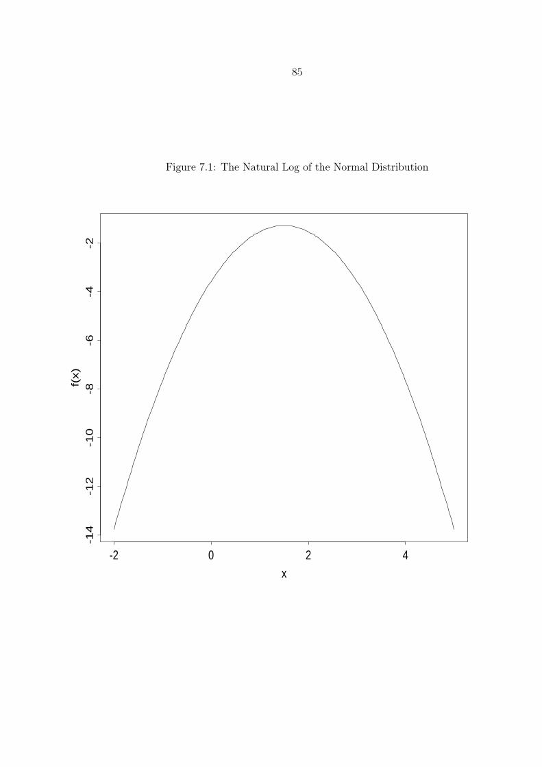
85

Figure 7.1: The Natural Log of the Normal Distribution

x

f(x)

-2 0 2 4

-14

-12

-10

-8-6

-4-2

86

Part III

Models for Repeated ObservationsData—Continuous Dependent Variables

Section 8

Fixed Effects Estimators

8.1 LSDV as Fixed Effects

• Least squares dummy variable estimation is also known as fixed effects,because it assumes that the unobserved effect for a given cross-sectional unitor time period can be estimated as a given, fixed effect.

• Can think of this as fixed in repeated samples (e.g., France is France) asopposed to randomly drawn.

• Let the original model be

yit = α∗i + β′xit + uit (8.1)

87

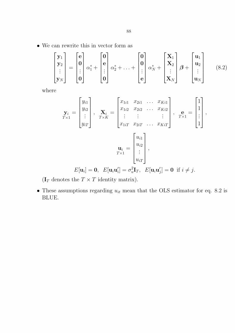
88

• We can rewrite this in vector form asy1

y2...

yN

=

e0...0

α∗1 +

0e...0

α∗2 + . . .+

00...e

α∗N +

X1

X2...

XN

β +

u1

u2...

uN

(8.2)

where

yiT×1

=

yi1

yi2...yiT

, XiT×K

=

x1i1 x2i1 . . . xKi1

x1i2 x2i2 . . . xKi2...

......

x1iT x2iT . . . xKiT

, eT×1

=

11...1

,

uiT×1

=

ui1

ui2...uiT

,E[ui] = 0, E[uiu

′i] = σ2

uIT , E[uiu′j] = 0 if i 6= j.

(IT denotes the T × T identity matrix).

• These assumptions regarding uit mean that the OLS estimator for eq. 8.2 isBLUE.

89

• To obtain the OLS estimators of α∗i and β, we minimize:

S =N∑

i=1

u′iui =N∑

i=1

(yi − eα∗i −Xiβ)′(yi − eα∗i −Xiβ).

• Take partial derivatives wrt to α∗i , set equal to zero and solve to get:

α∗i = yi − β′xi (8.3)

where

yi =T∑

t=1

yit/T, xi =T∑

t=1

xit/T, .

• Substitute our estimate for α∗i in S, take partial derivatives wrt β, set equalto zero and solve:

βCV =

[N∑

i=1

T∑t=1

(xit − xi)(xit − xi)′

]−1 [ N∑i=1

T∑t=1

(xit − xi)(yit − yi)

]

• Including separate dummies for each cross-sectional unit will produce esti-mates of the unit-specific effects.

• While this may be desirable, it does come at some cost—possibly inverting alarge matrix of 0s and 1s.

90

• Another way to compute this estimator w/o including dummies is to subtractoff the time means:

yi = α∗i + β′xi + ui (8.4)

• If we run OLS on this regression, it will produce what is known as the “Be-tween Effects” estimator, or βBE, which shows how the mean level of thedependent variable for each cross-sectional unit varies with the mean level ofthe independent variables.

• Subtracting eq. 8.4 from eq. 8.1 gives

(yit − yi) = (α∗i − α∗i ) + β′(xit − xi) + (uit − ui)

or(yit − yi) = β′(xit − xi) + (uit − ui)

• Running OLS on this equation gives results identical to LSDV.

• Sometimes called the within-group estimator, because it uses only the varia-tion in yit and xit within each cross-sectional unit to estimate the β coeffi-cients.

• Any variation between cross-sectional units is assumed to spring from theunobserved fixed effects.

91

• Another way to approach this is to pre-multiply each cross-sectional unitequation (yi = eα∗i + Xiβ + ui) by a T × T idempotent “sweep” matrix:

Q = It −1

Tee′

• This has the effect of sweeping out the α∗i s and transforming the variables sothat the values for each individual are measured in terms of deviations fromtheir means over time:

Qyi = Qeα∗i + QXiβ + Qui (8.5)

= QXiβ + Qui (8.6)

• Running OLS on this regression gives

βCV =

[N∑

i=1

X′iQXi

]−1 [ N∑i=1

XiQyi

]

• The variance-covariance matrix is

var[βCV] = σ2u

[N∑

i=1

X′iQXi

]−1

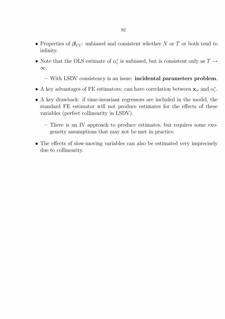
92

• Properties of βCV: unbiased and consistent whether N or T or both tend toinfinity.

• Note that the OLS estimate of α∗i is unbiased, but is consistent only as T →∞.

– With LSDV consistency is an issue: incidental parameters problem.

• A key advantages of FE estimators: can have correlation between xit and α∗i .

• A key drawback: if time-invariant regressors are included in the model, thestandard FE estimator will not produce estimates for the effects of thesevariables (perfect collinearity in LSDV).

– There is an IV approach to produce estimates, but requires some exo-geneity assumptions that may not be met in practice.

• The effects of slow-moving variables can also be estimated very impreciselydue to collinearity.

93

8.2 Application: Economic growth in 14 OECD countries

• Garrett examines the political component of economic performance in his ’98book Partisan Politics in the Global Economy.

• Question: how does labor centralization and left control of the governmentaffect economic growth (esp. in terms of an interaction effect)?

– Tests the social democratic corporatist model of economic performance:congruence b/t political and labor bargaining enhances performance.

– I.e., centralized labor bargaining goes well w/ politically powerful leftparties; decentralized bargaining is more congruent when right partiesare in power.

• Data: 14 OECD countries observed annually from 1966–1990 (i.e., N =14;T = 25.

• Dependent variable: GDP.

• Explanatory vars:

– Oil dependence (OIL),

– Overall OECD GDP growth, weighted for each country by its trade withthe other OECD nations (DEMAND),

– proportion of cabinet posts occupied by left parties (LEFTLAB),

– degree of centralized labor bargaining as a measure of corporatism (CORP),

– interaction b/t CORP and LEFTLAB (CLINT).

94

• OLS on this equation gives:

. regress gdp oild demand corp leftlab clint

Source | SS df MS Number of obs = 350

-------------+------------------------------ F( 5, 344) = 11.30

Model | 291.283034 5 58.2566069 Prob > F = 0.0000

Residual | 1773.90603 344 5.15670357 R-squared = 0.1410

-------------+------------------------------ Adj R-squared = 0.1286

Total | 2065.18906 349 5.91744717 Root MSE = 2.2708

------------------------------------------------------------------------------

gdp | Coef. Std. Err. t P>|t| [95% Conf. Interval]

-------------+----------------------------------------------------------------

oild | -15.2321 4.572497 -3.33 0.001 -24.22567 -6.238529

demand | .0049977 .000999 5.00 0.000 .0030328 .0069625

corp | -1.139716 .3043989 -3.74 0.000 -1.738433 -.5409982

leftlab | -1.483549 .3844653 -3.86 0.000 -2.239747 -.7273499

clint | .4547183 .1233779 3.69 0.000 .2120482 .6973883

_cons | 5.919865 .7356383 8.05 0.000 4.47295 7.36678

------------------------------------------------------------------------------

95

• Including dummies for each country (except one) gives:

. regress gdp oild demand corp leftlab clint Icc_2 Icc_3 Icc_4 Icc_5 Icc_6 Icc_

> 7 Icc_8 Icc_9 Icc_10 Icc_11 Icc_12 Icc_13 Icc_14;

Source | SS df MS Number of obs = 350

-------------+------------------------------ F( 18, 331) = 9.16

Model | 686.921905 18 38.1623281 Prob > F = 0.0000

Residual | 1378.26716 331 4.16394912 R-squared = 0.3326

-------------+------------------------------ Adj R-squared = 0.2963

Total | 2065.18906 349 5.91744717 Root MSE = 2.0406

------------------------------------------------------------------------------

gdp | Coef. Std. Err. t P>|t| [95% Conf. Interval]

-------------+----------------------------------------------------------------

oild | -25.59808 5.946569 -4.30 0.000 -37.29592 -13.90025

demand | .0084949 .001129 7.52 0.000 .006274 .0107158

corp | -.2500641 .6654194 -0.38 0.707 -1.559048 1.05892

leftlab | -1.172257 .4468775 -2.62 0.009 -2.051335 -.2931785

clint | .5030912 .1596682 3.15 0.002 .1889988 .8171836

Icc_2 | -.4136903 .5988751 -0.69 0.490 -1.591772 .7643909

Icc_3 | -2.090873 .7898403 -2.65 0.009 -3.644613 -.5371336

Icc_4 | -2.159732 .7633224 -2.83 0.005 -3.661307 -.658157

Icc_5 | -2.587796 1.091167 -2.37 0.018 -4.734293 -.4412985

Icc_6 | .6289216 .8440104 0.75 0.457 -1.031379 2.289222

Icc_7 | -1.796217 1.255454 -1.43 0.153 -4.265892 .6734584

Icc_8 | -3.993015 1.891938 -2.11 0.036 -7.714754 -.2712759

Icc_9 | -.8709414 1.02877 -0.85 0.398 -2.894693 1.15281

Icc_10 | -1.449112 1.301281 -1.11 0.266 -4.008935 1.110711

Icc_11 | -3.893792 1.607724 -2.42 0.016 -7.056438 -.7311463

Icc_12 | -3.489515 1.29017 -2.70 0.007 -6.027481 -.9515491

Icc_13 | -3.10808 1.477907 -2.10 0.036 -6.015355 -.200806

Icc_14 | 2.929627 .6076861 4.82 0.000 1.734213 4.125041

_cons | 3.374094 1.365808 2.47 0.014 .6873365 6.060852

------------------------------------------------------------------------------

96

• The F -test to determine if the dummies should be included gives:

. test Icc_2=Icc_3=Icc_4=Icc_5=Icc_6=Icc_7=Icc_8=Icc_9=Icc_10=Icc_11=Icc_12=Icc

> _13=Icc_14=0;

F( 13, 331) = 7.31

Prob > F = 0.0000

• Finally, estimating the fixed effects model:

. xtreg gdp oild demand corp leftlab clint, fe ;

Fixed-effects (within) regression Number of obs = 350

Group variable (i): country Number of groups = 14

R-sq: within = 0.2315 Obs per group: min = 25

between = 0.0461 avg = 25.0

overall = 0.0424 max = 25

F(5,331) = 19.94

corr(u_i, Xb) = -0.7104 Prob > F = 0.0000

------------------------------------------------------------------------------

gdp | Coef. Std. Err. t P>|t| [95% Conf. Interval]

-------------+----------------------------------------------------------------

oild | -25.59808 5.946569 -4.30 0.000 -37.29592 -13.90025

demand | .0084949 .001129 7.52 0.000 .006274 .0107158

corp | -.2500641 .6654194 -0.38 0.707 -1.559048 1.05892

leftlab | -1.172257 .4468775 -2.62 0.009 -2.051335 -.2931785

clint | .5030912 .1596682 3.15 0.002 .1889988 .8171836

_cons | 1.78165 1.961666 0.91 0.364 -2.077255 5.640556

-------------+----------------------------------------------------------------

sigma_u | 1.9296773

sigma_e | 2.0405757

rho | .47208946 (fraction of variance due to u_i)

------------------------------------------------------------------------------

F test that all u_i=0: F(13, 331) = 7.31 Prob > F = 0.0000

Section 9

Random Effects Estimators

9.1 Intro

• Fixed effects is completely appropriate if we believe that the unit-specificeffects are indeed fixed, estimable amounts that we can calculate for eachcross-sectional observation.

• Thus, we believe that Sweden will always have an intercept of 1.2 units (forinstance). If we were able to take another sample, we would once againestimate the same intercept for Sweden. There are cases, however, where wemay not believe that we can estimate some fixed amount for each country.

• In particular, assume that we have a panel data model run on 20 countries,but which should be generalizable to 100 different countries. We cannotestimate the given intercept for each country or each type of country becausewe don’t have all of them in the sample for which we estimate the model.

• In this case, we might want to estimate the βs on the explanatory variablestaking into account that there could be country-specific effects that wouldenter as a random shock from a known distribution.

• If we go this route, we will be estimating a random effects model.

97

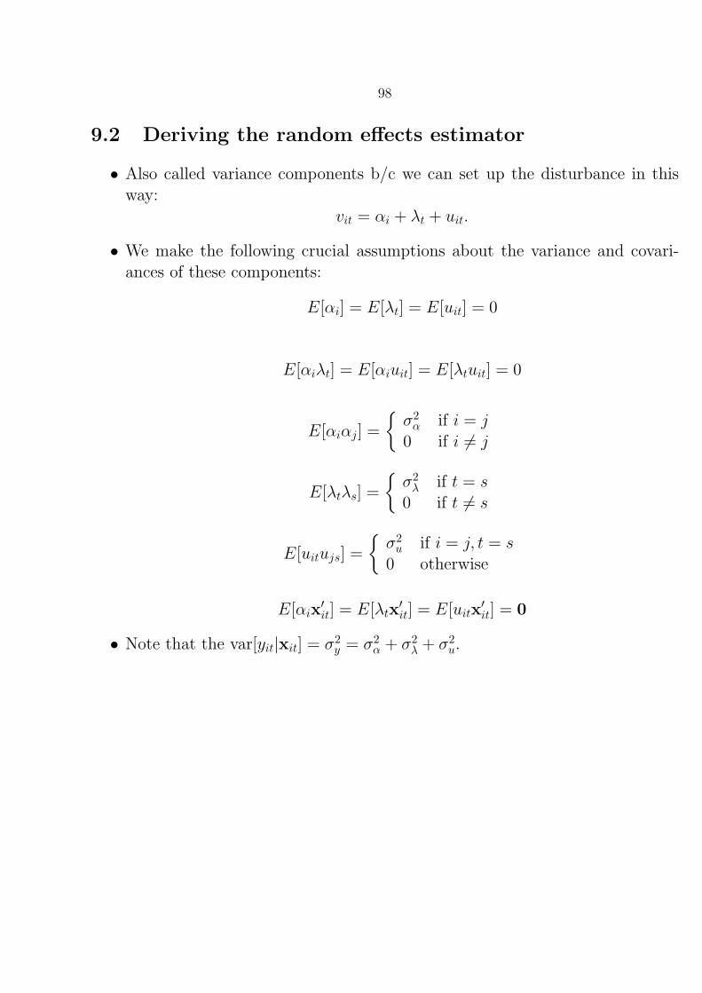
98

9.2 Deriving the random effects estimator

• Also called variance components b/c we can set up the disturbance in thisway:

vit = αi + λt + uit.

• We make the following crucial assumptions about the variance and covari-ances of these components:

E[αi] = E[λt] = E[uit] = 0

E[αiλt] = E[αiuit] = E[λtuit] = 0

E[αiαj] =

σ2

α if i = j

0 if i 6= j

E[λtλs] =

σ2

λ if t = s

0 if t 6= s

E[uitujs] =

σ2

u if i = j, t = s

0 otherwise

E[αix′it] = E[λtx

′it] = E[uitx

′it] = 0

• Note that the var[yit|xit] = σ2y = σ2

α + σ2λ + σ2

u.

99

• Let’s add a general intercept to our model and set λt = 0 ∀ t:

yit = µ+ β′xit + αi + uit (9.1)

• We can rewrite this in vector form:

yi = Xiδ + vi (9.2)

where

XiT×(K+1)

=[e Xi

], δ

(K+1)×1=

[µ

β

], vi

T×1=

vi1

vi2...viT

, vit = αi + uit

• The variance-covariance matrix of the T disturbance terms vi is:

V = E[viv′i] =

(σ2

u + σ2α) σ2

α σ2α . . . σ2

α

σ2α (σ2

u + σ2α) σ2

α . . . σ2α

... . . . ...σ2

α σ2α σ2

α . . . (σ2u + σ2

α)

= σ2

uIT + σ2αee

′

• Note that

V−1 =1

σ2u

[IT −

σ2α

σ2u + Tσ2

α

]ee′.

• The full variance-covariance matrix for all the NT observations is:

Ω =

V 0 0 . . . 00 V 0 . . . 0... . . . ...0 0 0 . . . V

= IN ⊗V

100

• To produce parameter estimates, we could proceed in the manner that wedid with the FE estimator—i.e., pre-multiply by Q and run OLS.

– This will give unbiased and consistent estimates.

– However, if the αi are assumed to be random rather than fixed, the CVestimator is not BLUE; the GLS estimator is.

– Intuition: vit and vis both contain αi, inducing correlation in the distur-bances. Need to use GLS to get efficient estimates.

9.3 GLS Estimation

• The normal equations for the GLS estimator are[N∑

i=1

X′iV

−1Xi

]δGLS =

N∑i=1

XiV−1yi

• We could write the GLS estimator simply as

δGLS =

[N∑

i=1

X′iV

−1Xi

]−1 N∑i=1

XiV−1yi (9.3)

• But let’s unpack this to get a better understanding of what is going on w/this estimator. We can rewrite the inverse of the variance-covariance matrixas

V−1 =1

σ2u

[IT −

1

Tee′ + ψ · 1

Tee′]

=1

σ2u

[Q + ψ · 1

Tee′]

where

ψ =σ2

u

σ2u + Tσ2

α

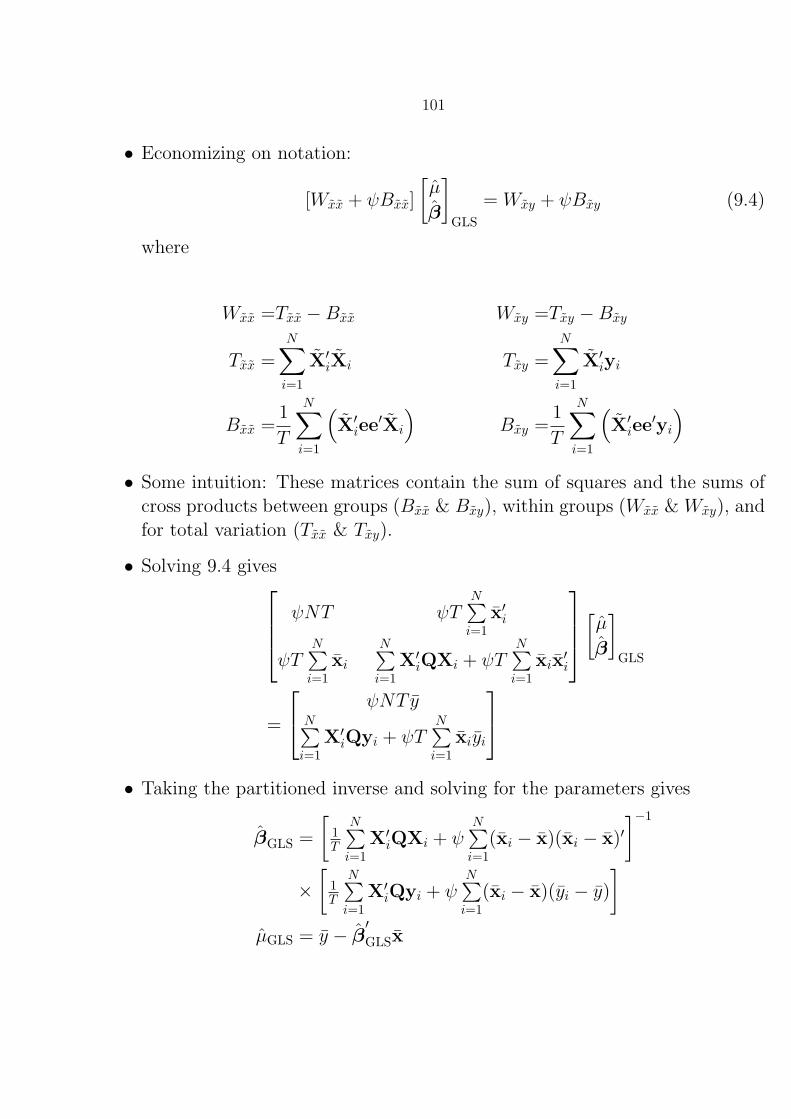
101

• Economizing on notation:

[Wxx + ψBxx]

[µ

β

]GLS

= Wxy + ψBxy (9.4)

where

Wxx =Txx −Bxx Wxy =Txy −Bxy

Txx =N∑

i=1

X′iXi Txy =

N∑i=1

X′iyi

Bxx =1

T

N∑i=1

(X′

iee′Xi

)Bxy =

1

T

N∑i=1

(X′

iee′yi

)• Some intuition: These matrices contain the sum of squares and the sums of

cross products between groups (Bxx & Bxy), within groups (Wxx & Wxy), andfor total variation (Txx & Txy).

• Solving 9.4 gives ψNT ψTN∑

i=1x′i

ψTN∑

i=1xi

N∑i=1

X′iQXi + ψT

N∑i=1

xix′i

[µβ]

GLS

=

ψNT yN∑

i=1X′

iQyi + ψTN∑

i=1xiyi

• Taking the partitioned inverse and solving for the parameters gives

βGLS =

[1T

N∑i=1

X′iQXi + ψ

N∑i=1

(xi − x)(xi − x)′]−1

×[

1T

N∑i=1

X′iQyi + ψ

N∑i=1

(xi − x)(yi − y)

]µGLS = y − β

′GLSx

102

• We can rewrite βGLS as∆βb + (Ik −∆)βCV

where

∆ = ψT

[N∑

i=1

X′iQXi + ψT

N∑i=1

(xi − x)(xi − x)′

]−1

×

[N∑

i=1

(xi − x)(xi − x)′

],

βb =

[N∑

i=1

(xi − x)(xi − x)′

]−1 [ N∑i=1

(xi − x)(yi − y)

].

• In words: the GLS estimator is a weighted average of the b/t group estimatorand the w/in group estimator, w/ ψ indicating the weight given to b/t groupvariation. Recall

ψ =σ2

u

σ2u + Tσ2

α

– As ψ → 1, δGLS → T−1xx Txy (i.e., the OLS estimator). This means that

little variance is explained by the unit effects.

– As ψ → 0, βGLS → the w/in estimator. This happens as either

1. the unit-specific effects dominate the disturbance uit.

2. T → ∞ (intuition: the αi are like fixed parameters since we have somuch data on the T dimension).

– GLS then is an intermediate approach b/t OLS and FE (which uses nob/t group variation).

103

• The variance of the GLS estimator is

var[βGLS

]= σ2

u

[N∑

i=1

X′iQXi + ψT

N∑i=1

(xi − x)(xi − x)′

]−1

• Recall the variance for the w/in group estimator:

var[βCV] = σ2u

[N∑

i=1

X′iQXi

]−1

.

• The difference b/t these var-cov matrices is a p.d. matrix (assuming ψ > 0).

• Thus, as T →∞, ψ → 0, and var[√

T βGLS

]→ var

[√T βCV

](assuming our

cross-product matrices converge to finite p.d. matrices).

• Since we typically do not know σ2u and σ2

α, they must be estimated. We cando two-step GLS (i.e., obtain consistent estimates of the variance componentsand then plug these in to compute 2nd stage parameter estimates).

• If either N →∞ or T →∞, 2-step GLS has the same asymptotic propertiesas GLS w/ known variance components.

• Can use w/in and b/t group residuals to compute estimates:

σ2u =

N∑i=1

T∑t=1

[(yit − yi)− β

′CV(xit − xi)

]2N(T − 1)−K

(9.5)

σ2α =

N∑i=1

[yi − µ− β′xi

]2N − (K + 1)

− 1

Tσ2

u (9.6)

where µ and β are obtained from B−1xxBxy.

104

9.4 Maximum Likelihood Estimation

• RE estimates can also be computed by ML.

• To obtain the MLE, assume uit and αi are normally dist’d and start w/ thelog of the likelihood function:

lnL = −NT2

ln 2π − N

2ln |V|

− 1

2

N∑i=1

(yi − eµ−Xiβ)′V−1(yi − eµ−Xiβ)

• To obtain the MLE δ′= (µ,β′, σ2

u, σ2α), we take partial derivatives wrt each

of these parameters, set to zero and solve.

• This gives four equations that we must solve simultaneously, which can bedifficult.

• Instead we can use a sequential iterative procedure, alternating back andforth b/t µ and β and the variance components σ2

u and σ2α.

• For N fixed and T →∞, the MLEs of µ,β′, and σ2u are consistent and → CV

estimator. The MLE of σ2α is inconsistent (insufficient variation b/c of fixed

N).

• With simultaneous solution of σ2α, it’s possible to obtain a negative value. It’s

also possible to obtain a boundary solution, although the prob. of this → 0as either T or N →∞.

105

9.5 Fixed v. Random Effects

• Makes no difference for large T .

• Can make a big difference when T is fixed and N is large.

• Does it make sense to treat one source of unobserved variation as random(uit) and another as fixed (αi)?

• Conditional v. marginal inference:

– FE is often thought of as an approach where inferences are made condit’lon effects that are in the sample.

– RE can be thought of as making inferences that are unconditional ormarginal wrt the pop. of all effects.

• Perhaps the most important consideration is whether we think the unit ef-fects are correlated w/ explanatory variables—if so, RE is not appropriate(although may not make much difference in certain situations).

9.6 Testing between Fixed and Random Effects

• If αi is uncorrelated with the explanatory variables xit:

– GLS is unbiased/consistent and will achieve the Cramer-Rao lower bound(i.e., is efficient).

– CV is unbiased/consistent but is inefficient.

• If αi is correlated with any of the explanatory variables:

– GLS is biased/inconsistent.

– CV is unbiased/consistent.

106

• This sets us up for a Hausman test:

H0: E[αixit] = 0; Random effects appropriate ⇒ βGLS is approx-imately equal to βCV but is more efficient (has smaller standarderrors).

H1: E[αixit] 6= 0; Random effects is not appropriate ⇒ βGLS will bedifferent from βCV (and inconsistent).

• In this setting, the Hausman test statistic is calculated as:

m = (βCV − βGLS)′(var[βCV]− var[βGLS]

)−1(βCV − βGLS)

• m ∼ χ2K .

• If m is larger than its appropriate critical value, then we reject random effectsas the appropriate specification.

107

9.7 Application

• Let’s try random effects on the Garrett data:

xtreg gdp oild demand corp leftlab clint, re ;

Random-effects GLS regression Number of obs = 350

Group variable (i): country Number of groups = 14

R-sq: within = 0.2225 Obs per group: min = 25

between = 0.0007 avg = 25.0

overall = 0.1255 max = 25

Random effects u_i ~ Gaussian Wald chi2(5) = 87.18

corr(u_i, X) = 0 (assumed) Prob > chi2 = 0.0000

------------------------------------------------------------------------------

gdp | Coef. Std. Err. z P>|z| [95% Conf. Interval]

-------------+----------------------------------------------------------------

oild | -20.44602 5.394257 -3.79 0.000 -31.01857 -9.873467

demand | .0075601 .0010875 6.95 0.000 .0054286 .0096915

corp | -1.210037 .420998 -2.87 0.004 -2.035178 -.3848961

leftlab | -1.256097 .4275844 -2.94 0.003 -2.094147 -.4180465

clint | .4653267 .1481581 3.14 0.002 .1749422 .7557112

_cons | 5.19839 1.111886 4.68 0.000 3.019134 7.377646

-------------+----------------------------------------------------------------

sigma_u | .98722663

sigma_e | 2.0405757

rho | .18966702 (fraction of variance due to u_i)

------------------------------------------------------------------------------

• Note the big differences in the coefficient values compared w/ FE (for FGLSMLE, replace re w/ mle).

108

• Let’s run a Hausman test. The commands for this model would be

xtreg gdp oild demand corp leftlab clint, fe ;

est store garrettfe ;

xtreg gdp oild demand corp leftlab clint, re ;

est store garrettre ;

hausman garrettfe garrettre;

• The results:

---- Coefficients ----

| (b) (B) (b-B) sqrt(diag(V_b-V_B))

| garrettfe garrettre Difference S.E.

-------------+----------------------------------------------------------------

oild | -25.59808 -20.44602 -5.152068 2.502733

demand | .0084949 .0075601 .0009349 .0003033

corp | -.2500641 -1.210037 .9599731 .5153092

leftlab | -1.172257 -1.256097 .0838399 .1298888

clint | .5030912 .4653267 .0377645 .0595242

------------------------------------------------------------------------------

b = consistent under Ho and Ha; obtained from xtreg

B = inconsistent under Ha, efficient under Ho; obtained from xtreg

Test: Ho: difference in coefficients not systematic

chi2(5) = (b-B)’[(V_b-V_B)^(-1)](b-B)

= 15.39

Prob>chi2 = 0.0088

Section 10

Non-Spherical Errors

10.1 Introduction

• Up to this point, we have assumed that our errors were spherical.

• A good deal of attention, however, has been paid to issues of non-sphericalerrors in panel and TSCS data (esp. the latter).

10.2 The Method of PCSEs

• Key motivation for using panel corrected standard errors (PCSEs): improveinferences made from TSCS data by taking into account the complexity ofthe error process, but not ask too much of data.

• Non-standard error structures (TSCS):

1. Contemporaneous correlation: errors across cross-sect’l units are corre-lated due to common shocks in a given time period.

E(uit, ujs) =

σ2

i if i = j and s = t

σij if i 6= j and s = t

0 otherwise

2. Panel heteroskedasticity: error var. differs across cross-sect’l units dueto characteristics unique to the units.

E(uit, ujs) =

σ2

i if i = j and s = t

0 otherwise

3. Serial correlation: errors w/ units are temporally correlated.

uit = ρui,t−1 + εit.

109

110

• OLS not BLUE & can produce incorrect SEs when the errors are nonspherical.

• GLS is BLUE & gives correct SEs.

• But assumes that the var-cov matrix (Ω), used to weight the data is known.

• Can do FGLS using Ω.

• Beck & Katz ’95 APSR show, however, that the FGLS method advocated byParks and Kmenta produces incorrect SEs when applied to TSCS data.

• FGLS gives overconfident SEs—does not fully take into account the variabil-ity in the estimates of the error parameters (rely too heavily on asymptoticproperties).

• Beck & Katz ’95 APSR: superior way to handle complex error structures w/TSCS analysis is to estimate coefficients by OLS & compute PCSEs.

• Intuition: OLS with TSCS data will be unbiased but will produce incorrectstandard errors.

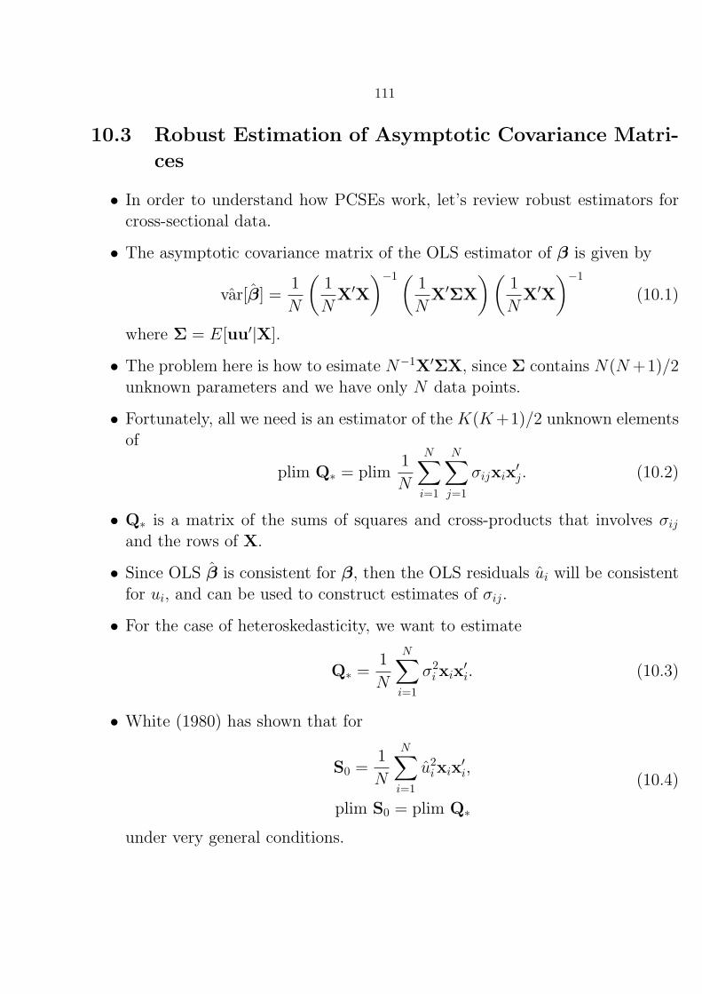
111

10.3 Robust Estimation of Asymptotic Covariance Matri-

ces

• In order to understand how PCSEs work, let’s review robust estimators forcross-sectional data.

• The asymptotic covariance matrix of the OLS estimator of β is given by

var[β] =1

N

(1

NX′X

)−1(1

NX′ΣX

)(1

NX′X

)−1

(10.1)

where Σ = E[uu′|X].

• The problem here is how to esimate N−1X′ΣX, since Σ contains N(N+1)/2unknown parameters and we have only N data points.

• Fortunately, all we need is an estimator of the K(K+1)/2 unknown elementsof

plim Q∗ = plim1

N

N∑i=1

N∑j=1

σijxix′j. (10.2)

• Q∗ is a matrix of the sums of squares and cross-products that involves σij

and the rows of X.

• Since OLS β is consistent for β, then the OLS residuals ui will be consistentfor ui, and can be used to construct estimates of σij.

• For the case of heteroskedasticity, we want to estimate

Q∗ =1

N

N∑i=1

σ2i xix

′i. (10.3)

• White (1980) has shown that for

S0 =1

N

N∑i=1

u2ixix

′i,

plim S0 = plim Q∗

(10.4)

under very general conditions.

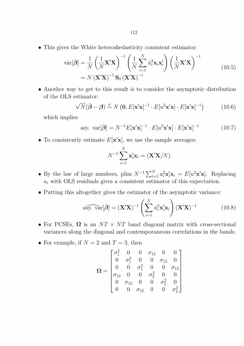
112

• This gives the White heteroskedasticity consistent estimator:

var[β] =1

N

(1

NX′X

)−1(

1

N

N∑i=1

u2ixix

′i

)(1

NX′X

)−1

= N (X′X)−1

S0 (X′X)−1

(10.5)

• Another way to get to this result is to consider the asymptotic distributionof the OLS estimator:

√N(β − β)

a∼ N(0, E[x′x]−1 · E[u2x′x] · E[x′x]−1) (10.6)

which implies

asy. var[β] = N−1E[x′x]−1 · E[u2x′x] · E[x′x]−1 (10.7)

• To consistently estimate E[x′x], we use the sample averages:

N−1N∑

i=1

x′ixi = (X′X/N).

• By the law of large numbers, plim N−1∑Ni=1 u

2ix

′ixi = E[u2x′x]. Replacing

ui with OLS residuals gives a consistent estimator of this expectation.

• Putting this altogether gives the estimator of the asymptotic variance:

asy. var[β] = (X′X)−1

(N∑

i=1

u2ix

′ixi

)(X′X)−1 (10.8)

• For PCSEs, Ω is an NT × NT band diagonal matrix with cross-sectionalvariances along the diagonal and contemporaneous correlations in the bands.

• For example, if N = 2 and T = 3, then

Ω =

σ21 0 0 σ12 0 00 σ2

1 0 0 σ12 00 0 σ2

1 0 0 σ12

σ12 0 0 σ22 0 0

0 σ12 0 0 σ22 0

0 0 σ12 0 0 σ22

113

• More generally,

Ω =

σ2

1IT σ12IT · · · σ1NIT

σ21IT σ22IT · · · σ2NIT

... . . . ...σN1IT σN2IT · · · σ2

NIT

• Let

Σ =

σ2

1 σ12 σ13 · · · σ1N

σ12 σ22 σ23 · · · σ2N

... . . . ...σ1N σ2N σ3N · · · σ2

N

• Use OLS residuals, denoted eit for unit i at time t (in Beck and Katz’s nota-

tion), to estimate the elements of Σ:

Σij =

∑Tt=1 eitejt

T, (10.9)

which means the estimate of the full matrix Σ is

Σ =E′E

T

where E is a T ×N matrix of the re-shaped NT × 1 vector of OLS residuals,such that the columns contains the T × 1 vectors of residuals for each cross-sectional unit (or conversely, each row contains the N × 1 vector of residualsfor each cross-sectional in a given time period) :

E =

e11 e21 . . . eN1

e12 e22 . . . eN2...

... . . . ...e1T e2T . . . eNT

Then

Ω =E′E

T⊗ IT ,

114

• Compute SEs using the square roots of the diagonal elements of

(X′X)−1X′ΩX(X′X)−1, (10.10)

where X denotes the NT × k matrix of stacked vectors of explanatory vari-ables, xit.

• Intuition behind why PCSEs do well: similar to White’sheteroskedasticity-consistent standard errors for cross-sect’l estimators, butbetter b/c take advantage of info provided by the panel structure.

• Good small sample properties confirmed by Monte Carlo studies.

• Potential problems:

– Note that this methods ignores unit effects—doesn’t have to, though.

– PCSEs solves the problems of panel heteroskedasticity and contempo-raneous correlation—not serial correlation. Serial correlation must beremoved before applying this fix.

– How to correct for serial correlation? Lags are recommended, but that in-troduces a potential problem that we’ll discuss when we turn to dynamicspecifications.

– Can also do Prais-Winsten.

115

10.4 Costs of ignoring unit effects revisited

• A dispute has arisen about the value of FE estimators when theory tells youthat time-invariant random variables should be included in your specification—better to just do OLS w/ PCSEs?

• We can run into trouble if unit effects are present in the data, but we ignorethem for the sake of including time-invariant variables; the problem is thatwe don’t know for sure what the true specification is.

• Methods for robust standard error estimation can help shed light on thisquestion.

• Suppose the DGP is described by the following equation:

yit = β′xit + αi + uit, (10.11)

where αi indicate the unit effects and we assume uit is spherical.

• If we ignore the unit effects then we are estimating the above model with thedisturbance vit = αi + uit.

• If αi is correlated with xit, then this leads to bias and inconsistency in OLSestimates of β.

• If it is not correlated there can still be problems with inferences: relegatingαi to the disturbance term in essence induces serial correlation in the errors.

• The variance-covariance matrix for β is given by

var[β] = E[(X′X)−1X′vv′X(X′X)−1], (10.12)

where X and v are the xit and vit stacked over all i and t.

• Let Σ = E[X′vv′X]. For the case of repeated cross-sections, this can berewritten as

Σ = E

[∑i

∑j

∑t

∑s

xitvitvjsx′js

](10.13)

116

• If vit = αi + uit, then

Σ = E

[∑i

∑t

∑s

xitx′itv

2it

]+ 2E

[∑i

∑t>s

xitx′isα

2i

](10.14)

• Even if the uit are spherical, the standard OLS estimator for the variance-covariance matrix will be wrong, since the second term in eq. 10.14 will beignored if the αi are not accounted for in the model specification.

• PCSEs will also ignore this term, leading to wrong standard errors.

• Interestingly, this presents a problem particularly for time invariant variablesb/c the std. errs. for the coefficients on such variables will generally be toosmall, possibly leading to type I errors.

• Consider the second term of eq. 10.14 when xit = (xit zi):

2E

∑i

∑t 6=s

[xitxis xitzi

xiszi zizi

]α2

i

(10.15)

• It is possible that the xs are uncorrelated across cross-sectional units and timeperiods and are uncorrelated w/ the zs ⇒ 0s in the first diagonal elementand the off-diagonals—do not contribute anything to the standard errors inexpectation.

• However, the zs are perfectly correlated within i ⇒ positive number whenmultiplied by α2 ⇒ larger standard errors than what we would get from OLS.

• To confirm this analytical result, conduct Monte Carlo analysis: generate thedata with an explanatory variable, xit, and a unit effect, but then estimatea model that replaces the unit effect with a randomly generated zi, which isindependent of xit and the unit effect.

– This set-up mimicks a scenario where a researcher forsakes the FE ap-proach to include a time invariant variable, even though—unbeknown tothe researcher—the time invariant variable actually has no effect.

117

Table 10.1: Results from Monte Carlo experiments involving timeinvariant variables

No lag One lag Two lags

Mean OLS γ −0.005 −0.003 0.007Mean Between γ −0.002 0.000 0.007Proportion of sig. OLS γs 0.573 0.991 0.976Proportion of sig. OLS γs, PCSEs 0.693 0.972 0.949Proportion of sig. OLS γs, Robust 0.134 0.958 0.948Proportion of sig. Between γs 0.073 0.071 0.074% reject H0 of no autocorrelation 99 96 10

Notes: N = 15;T = 20. 1000 simulations each.

• We estimated the model via standard OLS as well as with PCSEs. To verifythat the problem is a kind of serial correlation induced by ommission of theunit effects, we computed standard errors that are robust to serial correlationusing

var(β) = (X′X)−1

(N∑

i=1

T∑t=1

T∑s=1

xitx′isvitvis

)(X′X)

−1, (10.16)

where the vit are the residuals from a pooled OLS regression.

118

10.5 Heteroskedasticity in FE and RE models

• If we treat the αi as random, then heteroskedasticity can occur if we have σ2αi

or σ2ui or both:

Vi = E[viv′i] = σ2

uiIT + σ2αiee

′

• To do GLS, we use Vi instead of V.

• Since we typically do not know either σ2αi or σ2

ui, we can resort to a 2-stepFGLS approach.

– Problem: cannot get a consistent estimate for σ2αi even as T → ∞; only

one realization of αi (incidental parameters).

– Can get a consistent estimate of σ2ui as T →∞.

– W/ finite T , cannot get consistent estimates of either σ2αi or σ2

ui, even ifN →∞.

– If N and T are getting big, then we can get consistent estimates of σ2ui.

119

• To do FGLS:

1. Run OLS or CV on yi = Xiδ + vi and compute the estimated residualsvi.

2. Compute Vi either by

(a) assuming σ2αi = σ2

α ∀ i and using

σ2ui =

1

T − 1

T∑t=1

(vit − ˆvi

)2, (10.17)

or

(b) assuming the variance of αi conditional on xi has the same functionalform across individuals var[αi|xi] = σ2xi; σ

2ui is estimated as in eq.

10.17 (see Roy ’02 IER for a method of this type for heteroskedasticityof unknown form).

3. Then do

δFGLS =

[N∑

i=1

X′iV

−1i Xi

]−1 N∑i=1

XiV−1i yi

and approximate the asymptotic var-cov matrix of δFGLS by(N∑

i=1

X′iV

−1i Xi

)−1

• Could also do a feasible weighted LS method, weighting each obs. by thereciprocal of σui and then apply the CV estimator to the transformed data.

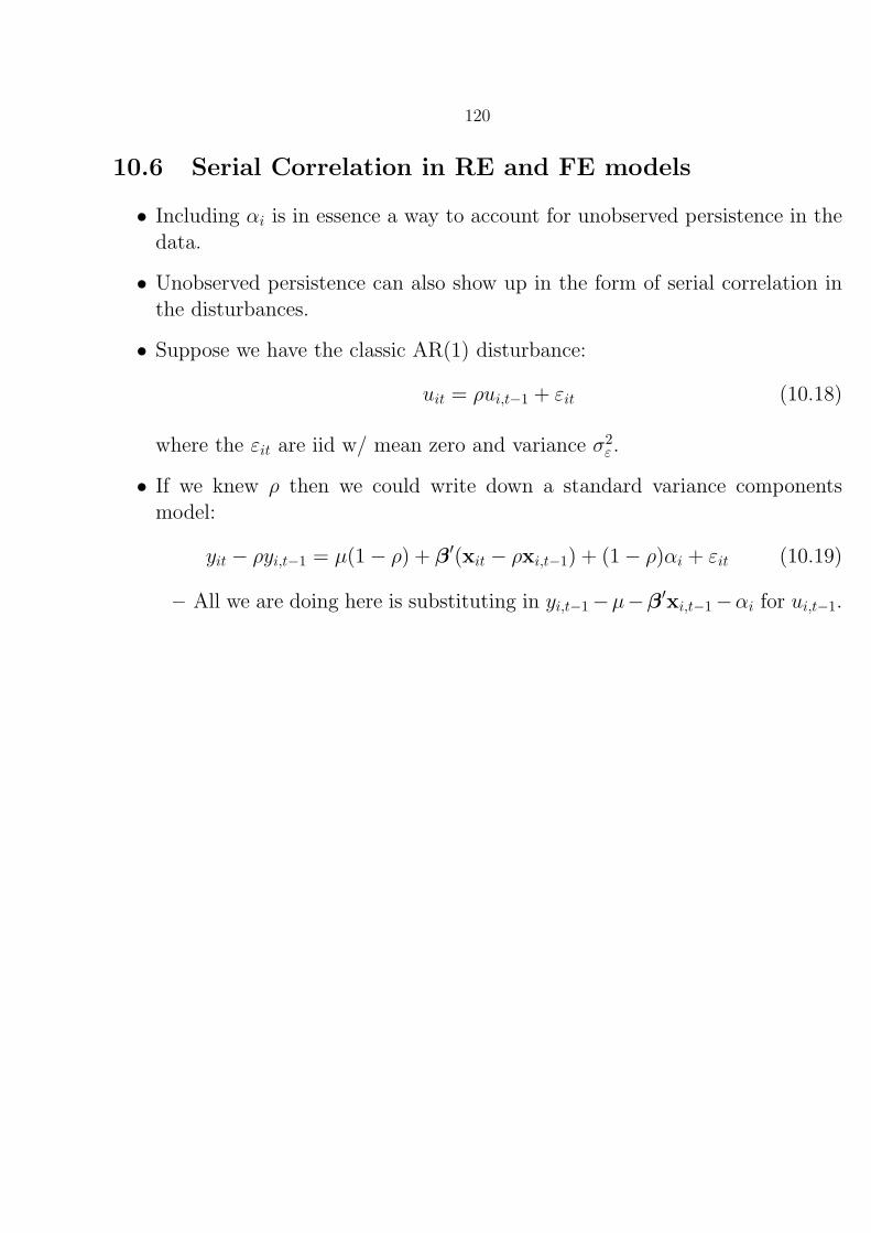
120

10.6 Serial Correlation in RE and FE models

• Including αi is in essence a way to account for unobserved persistence in thedata.

• Unobserved persistence can also show up in the form of serial correlation inthe disturbances.

• Suppose we have the classic AR(1) disturbance:

uit = ρui,t−1 + εit (10.18)

where the εit are iid w/ mean zero and variance σ2ε .

• If we knew ρ then we could write down a standard variance componentsmodel:

yit − ρyi,t−1 = µ(1− ρ) + β′(xit − ρxi,t−1) + (1− ρ)αi + εit (10.19)

– All we are doing here is substituting in yi,t−1−µ−β′xi,t−1−αi for ui,t−1.

121

• Can get an asymptotically efficient estimator of β by doing the following:

1. De-mean the data to take out the αi:

(yit − yi) = β′(xit − xi) + (uit − ui)

2. Compute an estimate of ρ:

(a) Use the LS residual from the de-meaned regression, or

(b) regress (yit−yi) on (yi,t−1−yi,−1) and (xi,t−1−xi,−1) and use the coeffi-

cient on (yi,t−1−yi,−1) as an estimate of ρ (note: yi,−1 = (1/T )T∑

t=1yi,t−1;

we assume we have measures of yi0 and xi0).

3. Compute estimates of σ2ε and σ2

α:

σ2ε =

1

NT

N∑i=1

T∑t=1

(yit − yi)− (1− ρ)µ− ρ(yi,t−1 − yi,−1)

− β′[(xit − xi)− (xi,t−1 − xi,−1)ρ]2

σ2α =

1

(1− ρ)2 ·1

N

N∑i=1

[yi − µ(1− ρ)− ρyi,−1 − β

′(xi − xi,−1ρ)

]2− 1

Tσ2

ε

Intuition: see equations for computing GLS variance estimates underassumption of spherical disturbances (i.e., eq. 9.5 and 9.6).

4. Plug in our estimate for ρ and use σ2ε and σ2

α to compute the var-covmatrix of (1− ρ)αi + εit.

122

10.7 Robust standard error estimation with unit effects

• The properties of the FGLS estimators just described depend crucially onasymptotics—may not do well in finite samples.

• Might be better off computing some kind of robust estimator of the var-covmatrix to get our standard errors (i.e., robust to both heteroskedasticity andserial correlation).

• Robust estimators for FE models exist; although they also rely on asymptoticproperties, they may do better in finite samples since they demand less of thedata.

10.7.1 Arellano robust standard errors

• Let y+i = Qyi, X+

i = QXi, u+i = Qui.

• Arellano (’87 Oxford Bulletin of Economics and Statistics) suggests the fol-lowing robust estimator:

(X+′X+)−1

(N∑

i=1

X+′i u+

i u+′i X+

i

)(X+′X+)−1

(10.20)

where u+i are the estimated residuals obtained from running OLS on the

transformed equation (i.e., u+i = y+

i −X+i βCV).

123

10.7.2 Kiefer robust standard errors

• Arellano also suggests (following Kiefer) the robust estimator:

(X+′X+)−1

(N∑

i=1

X+′i Ω

+i X+

i

)(X+′X+)−1

(10.21)

where

Ω+i =

1

N

N∑i=1

u+i u+′

i

• Both of these estimators assume T fixed and N →∞.

• In some Monte Carlo work I’ve done, the Arellano estimator does better thanKiefer for TSCS data.

• FE robust std. errs. can be obtained in Stata by using the robust andcluster options in the xtreg routine.

• Note that the Arellano approach is essentially the same as doing LSDV andthen computing PCSEs.

124

10.8 Application: Garrett data

• The Garrett model of GDP growth estimated w/ OECD data is exactly thekind of case where we might expect non-spherical errors.

. xtpcse gdp oild demand corp leftlab clint ;

Linear regression, correlated panels corrected standard errors (PCSEs)

Group variable: country Number of obs = 350

Time variable: year Number of groups = 14

Panels: correlated (balanced) Obs per group: min = 25

Autocorrelation: no autocorrelation avg = 25

max = 25

Estimated covariances = 105 R-squared = 0.1410

Estimated autocorrelations = 0 Wald chi2(5) = 42.01

Estimated coefficients = 6 Prob > chi2 = 0.0000

------------------------------------------------------------------------------

| Panel-corrected

gdp | Coef. Std. Err. z P>|z| [95% Conf. Interval]

-------------+----------------------------------------------------------------

oild | -15.2321 5.228694 -2.91 0.004 -25.48015 -4.984049

demand | .0049977 .0015394 3.25 0.001 .0019804 .0080149

corp | -1.139716 .2234088 -5.10 0.000 -1.577589 -.7018424

leftlab | -1.483549 .2755847 -5.38 0.000 -2.023685 -.9434125

clint | .4547183 .0839526 5.42 0.000 .2901741 .6192624

_cons | 5.919865 .5833949 10.15 0.000 4.776432 7.063298

----------------------------------------------------------------------------

125

• PCSEs, correcting for serial correlation:

. xtpcse gdp oild demand corp leftlab clint, correlation(ar1) ;

Prais-Winsten regression, correlated panels corrected standard errors (PCSEs)

Group variable: country Number of obs = 350

Time variable: year Number of groups = 14

Panels: correlated (balanced) Obs per group: min = 25

Autocorrelation: common AR(1) avg = 25

max = 25

Estimated covariances = 105 R-squared = 0.1516

Estimated autocorrelations = 1 Wald chi2(5) = 31.55

Estimated coefficients = 6 Prob > chi2 = 0.0000

------------------------------------------------------------------------------

| Panel-corrected

gdp | Coef. Std. Err. z P>|z| [95% Conf. Interval]

-------------+----------------------------------------------------------------

oild | -13.77226 6.587739 -2.09 0.037 -26.684 -.8605317

demand | .0060806 .0016414 3.70 0.000 .0028635 .0092977

corp | -1.177445 .2934019 -4.01 0.000 -1.752502 -.6023874

leftlab | -1.46776 .3623476 -4.05 0.000 -2.177949 -.757572

clint | .4488461 .1112233 4.04 0.000 .2308525 .6668397

_cons | 5.814019 .807692 7.20 0.000 4.230972 7.397066

-------------+----------------------------------------------------------------

rho | .2958842

------------------------------------------------------------------------------

126

• Fixed effects w/ robust standard errors a la Arellano:

. xtreg gdp oild demand corp leftlab clint, fe robust cluster(country)

Fixed-effects (within) regression Number of obs = 350

Group variable (i): country Number of groups = 14

R-sq: within = 0.2315 Obs per group: min = 25

between = 0.0461 avg = 25.0

overall = 0.0424 max = 25

F(5,345) = 14.29

corr(u_i, Xb) = -0.7104 Prob > F = 0.0000

(Std. Err. adjusted for 14 clusters in country)

------------------------------------------------------------------------------

| Robust

gdp | Coef. Std. Err. t P>|t| [95% Conf. Interval]

-------------+----------------------------------------------------------------

oild | -25.59808 14.10159 -1.82 0.093 -56.06271 4.866543

demand | .0084949 .0020412 4.16 0.001 .0040851 .0129047

corp | -.2500641 .9970869 -0.25 0.806 -2.404139 1.904011

leftlab | -1.172257 .3593795 -3.26 0.006 -1.948649 -.3958644

clint | .5030912 .1346974 3.73 0.002 .2120951 .7940873

_cons | 1.78165 3.051424 0.58 0.569 -4.810551 8.373852

-------------+----------------------------------------------------------------

sigma_u | 1.9296773

sigma_e | 2.0405757

rho | .47208946 (fraction of variance due to u_i)

------------------------------------------------------------------------------

• Note that

areg gdp oild demand corp leftlab clint, absorb(country) cluster(country)

gives the same results.

127

• For kicks, let’s do FGLS:

. xtgls gdp oild demand corp leftlab clint, panels(correlated);

Cross-sectional time-series FGLS regression

Coefficients: generalized least squares

Panels: heteroskedastic with cross-sectional correlation

Correlation: no autocorrelation

Estimated covariances = 105 Number of obs = 350

Estimated autocorrelations = 0 Number of groups = 14

Estimated coefficients = 6 Time periods = 25

Wald chi2(5) = 108.70

Log likelihood = -627.671 Prob > chi2 = 0.0000

------------------------------------------------------------------------------

gdp | Coef. Std. Err. z P>|z| [95% Conf. Interval]

-------------+----------------------------------------------------------------

oild | -14.01453 2.347816 -5.97 0.000 -18.61616 -9.412892

demand | .0045992 .0008527 5.39 0.000 .0029279 .0062705

corp | -1.107322 .1370615 -8.08 0.000 -1.375958 -.8386865

leftlab | -1.247823 .1348838 -9.25 0.000 -1.512191 -.9834559

clint | .4114256 .0479446 8.58 0.000 .3174559 .5053952

_cons | 5.41023 .276808 19.55 0.000 4.867696 5.952763

------------------------------------------------------------------------------

128

Part IV

Qualitative and Limited DependentVariable Models Based on the Normal

Regression Model

Section 11

Introduction2 parts:

1. Latent model: what’s really going on.

2. Observation scheme: determines what we get to see.

• Latent model for an individual:

y∗i = β′xi + ui

where y∗i is a scalar, β =

β1...βk

, xi =

xi1...xik

, and ui ∼ N [0, σ2].

β′xi = [β1 · · · βk]

xi1...xik

= β1xi1 + β2xi2 + · · ·+ βkxik

11.1 Linear Regression Model

• Observation Scheme #1: yi = y∗i

• That is, we get to see everything, so we have the classic normal linear regres-sion model.

129

Section 12

Probit

• Observation Scheme #2:

yi =

1 if y∗i > 00 if y∗i ≤ 0

y∗i > 0 ⇒ β′xi + ui > 0 ⇒ ui > −β′xi

Pr(y∗i > 0|xi) = Pr(yi = 1|xi) = Pr(ui > −β′xi)

= Pr

(ui

σ> −β

′xi

σ

)• Given the distribution we’ve assumed for ui, we can rewrite this probability

as

Pr(yi = 1|xi) = 1− Φ

(−β

′xi

σ

)= Φ

(β′xi

σ

)=

1√2π

∫ β′xi/σ

−∞exp

(−u

2

2

)du

130

131

• Similarly

Pr(yi = 0|xi) = 1− Φ

(β′xi

σ

)• An identification issue: in the probit model we cannot estimate β and σ

separately because they enter as a ratio (only the ratio is identifiable). So wejust set σ2 = 1.

• The likelihood function for the probit model then is

L = Πni=1[Φ(β′xi

)]yi[1− Φ

(β′xi

)]1−yi

while the log likelihood is

lnL =n∑

i=1

yi ln Φ

(β′xi

)+ (1− yi) ln

[1− Φ

(β′xi

)]• Differentiating w.r.t. β gives

∂ lnL

∂β=

n∑i=1

yi − Φ(β′xi

)Φ(β′xi

) [1− Φ

(β′xi

)]φ (β′xi

)xi

• Taking the second derivatives gives

∂2 lnL

∂β∂β′= −

n∑i=1

φ

[yiφ+ Φβ′xi

Φ2 + (1− yi)φ− (1− Φ)β′xi

[1− Φ]2

]xix

′i

where φ = φ(β′xi

)and Φ = Φ

(β′xi

).

132

12.1 Interpretation of Coefficients

• Estimated coefficients from the probit models do not have the same interpre-tation as they do in the linear regression model.

• In the linear model:

yi = β′xi + ui so∂yi

∂xi= β

• In the probit model we have

∂ Pr(yi = 1|xi)

∂xi=∂Φ(β′xi)

∂xi= φ(β′xi)β

• The effect of a unit change in xik on the probability that yi = 1 depends onthe value of xik as well as the values of other explanatory variables in themodel.

• Note that to compute this probability you must choose some values for the xvariables (e.g., medians or means for the sample).

• Another standard technique is to set the explanatory variables equal to cer-tain values and then change the value of a particular variable of interest tosee how it changes the probability of an event occurring.

133

• To be thorough, one should report measures of uncertainty for marginal effects(see Herron “Post-Estimation Uncertainty in Limited Dependent VariableModels” ’00 Political Analysis).

• For example, we can use simulation methods to compute confidence intervalsfor predicted probabilities. To do this, we’re going to get a bit a Bayesian, by

assuming βa∼ N

(β, Σ

), where Σ denotes the estimated covariance matrix.

1. Estimate β and Σ.

2. Repeat the following steps S times (e.g., S = 1000), indexing each itera-tion by l.

(a) Draw a vector β from a multivariate normal distribution with meanvector β and covariance matrix Σ.

(b) Calculate and save pli = Φ

(β′xi

).

3. Use the percentiles of the distribution of pli, l = 1, . . . , S, to form confi-

dence intervals of the desired size (e.g., 0.025 and 0.975 percentiles for a95% confidence interval).

134

12.2 Goodness of fit measures

• We can use a Likelihood Ratio (LR) test to compute a goodness of fit statisticsimilar to the F statistic in the linear regression context that tests the nullhypothesis that all of the slope coefficients are simultaneously equal to zero.

• Let θ be a vector of parameters to be estimated and H0 specify some restric-tions on this vector. The LR test is given by

−2[ln LR − ln LU

]where LR and LU are the likelihood evaluated at θR (the restricted parametervector) and θU (the unrestricted parameter vector).

−2[ln LR − ln LU

]∼ χ2

k

where k is the number of restrictions imposed.

• For the null that the slope coefficients are equal to zero

ln LR = ln L0 = n0 ln(n0

n

)+ n1 ln

(n1

n

)where n is the sample size, n0 is the number of observations where y = 0 andn1 is the number of observations where y = 1

135

• Some packages will report a pseudo R2 statistic, which has a similar “goodnessof fit” interpretation as the R2 statistic in the linear regression context.

For example, the statistic

1− ln LU

ln L0

ranges between 0 and 1 as does R2 in the linear regression model.

• Most stats packages will also report some measure of how well the modeldoes at predicting the occurrence of an event, such as the percentage ofobservations which are “correctly classified”.

• Herron recommends using expected percent correctly predicted (ePCP), whichsurmounts some of the problems of using just percent correctly predicted.

ePCP =1

N

(N∑

yi=1

pi +N∑

yi=0

(1− pi)

)(12.1)

136

12.3 Voting Behavior Example

• Consider the following model of vote choice in congressional elections

yi = β′xi + ui

where

x2i = party identification match incumbent’s dummy

x3i = national economic performance, retrospective evaluation

x4i = personal financial situation, retrospective evaluation

x5i = recall incumbent’s name

x6i = recall challenger’s name

x7i = quality of challenger

• Table 12.1 reports the results of probit estimation of this model using datafrom the American National Election Survey (1982–1988).

• Table 12.2 reports marginal effects using derivatives.

• We can also report marginal effects by simulating probabilities of observingan event. For example, we first compute the probability of voting for anincumbent given that she does not face a quality challenger. For the probitestimates, this is

Pr(yi = 1|x7i = 0) =Φ(β1 + β2x2i + β3x3i + β4x4i + β5x5i + β6x6i + β7x7i)

=Φ(.184 + 1.355× 1− .114× .5 + .095× .5

+ .324× 0− .677× 0− .339× 0)

=.936

137

Then compute this probability given a quality challenger:

Pr(yi = 1|x7i = 1) = .881

Then the difference between these two gives the percentage increase

in the probability of voting for the incumbent when she does not face

a quality challenger (i.e., .936− .881 = .055).

138

Table 12.1: Probability of Voting for the Incumbent Mem-ber of Congress

variable Probit MLEs

Intercept .184(.058)

Party identification 1.35(.056)

National economic performance –.114(Retrospective Judgment) (.069)

Personal financial situation .095(Retrospective Judgment) (.068)

Recall incumbent’s name .324(.0808)

Recall challenger’s name –.677(.109)

Quality of challenger –.339(.073)

Notes: Standard errors in parentheses.N = 3341. −2 lnL = 760.629 Percent cor-rectly predicted = 78.5%

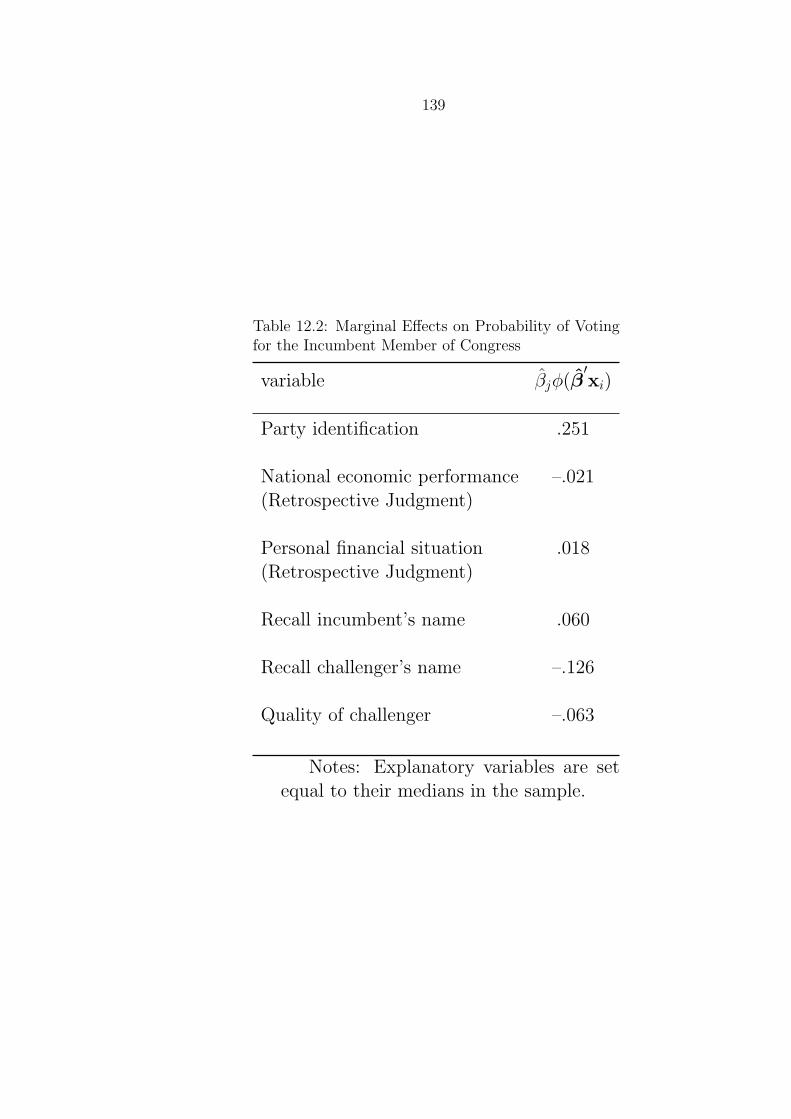
139

Table 12.2: Marginal Effects on Probability of Votingfor the Incumbent Member of Congress

variable βjφ(β′xi)

Party identification .251

National economic performance –.021(Retrospective Judgment)

Personal financial situation .018(Retrospective Judgment)

Recall incumbent’s name .060

Recall challenger’s name –.126

Quality of challenger –.063

Notes: Explanatory variables are setequal to their medians in the sample.

140

12.4 Obstruction and Passage of Legislation Example

We model the passage of legislation (yi = 1 if passed, = 0 if failed) as a functionof coalition sizes opposing obstruction of legislation in the U.S. Senate.

• Table 12.3 reports probit estimation results.

• Table 12.4 reports simulated probabilities (with confidence intervals) for spe-cific values of the coalition size variable.

• Figure 12.1 plots simulated probabilities (with confidence intervals) across arange of values for the coalition size variable.

141

Table 12.3: Probit analysis of passage of obstructed measures, 1st–64th Congresses

Variable Coefficient Std. Err.

Constant −1.671 0.962Coalition size 6.155 2.224Coalition size × end of session −1.944 0.690

Likelihood ratio test 12.84 (p = 0.002)% correctly predicted 72

Note: N = 114.

Table 12.4: Simulated Probabilities of Passage and Coalition Sizes, 1st–64th Congresses

Coalition size (%) Probability of PassageNot end of session End of session

51 .92 .67(.84, .97) (.47, .83)

60 .99 .80(.88, .99) (.54, .95)

67 .99 .87(.91, .99) (.54, .98)

Note: 95% confidence intervals in parentheses

142

Figure 12.1: Simulated Probabilities of Passage and Coalition Size

0.0 0.2 0.4 0.6 0.8 1.0

0.0

0.2

0.4

0.6

0.8

1.0

End of Congress

Coalition size

Pro

babi

lity

of p

assa

ge

0.0 0.2 0.4 0.6 0.8 1.0

0.0

0.2

0.4

0.6

0.8

1.0

Not End of Congress

Coalition size

Pro

babi

lity

of p

assa

ge

143

12.5 Heteroskedasticity and the Probit Model

• In the probit model heteroskedastic disturbances render the MLEs inconsis-tent and the variance-covariance matrix inappropriate.

• A general form of heteroskedasticity is

σ2i = exp(γ ′zi)

where zi = [1,qi] and γ = [lnσ2,α].

• The log likelihood for this heteroskedastic probit model is

lnL =n∑

i=1

yi ln Φ

(β′xi

exp(γ ′zi)

)+ (1− yi) ln

[1− Φ

(β′xi

exp(γ ′zi)

)](12.2)

• Note: qi should not contain a constant term.

• To test for heteroskedasticity we can use a LR test, where ln Lu is given by(12.2) and for ln LR we restrict γ = 0.

• A statistically significant χ2 statistic ⇒ heteroskedasticity is present.

144

• Application: Alvarez and Brehm, “American Ambivalence Towards Abor-tion Policy: Development of a Heteroskedastic Probit Model of CompetingValues.” ’95 AJPS.

• Individuals possess a variance of attitudes—variance stems from difficultyindividuals have in resolving conflict between “core” beliefs.

• Some individuals will have resolved such conflict to a greater degree thanothers—i.e., they will be less ambivalent.

• ambivalence = f(motivation and ability to process information, the degreethat the respondents evaluate the policy choice under both pro-life and pro-choice dimensions)

• Process that generates responses to questions about abortion policy is het-erogeneous ⇒ iid assumption may be incorrect.

• Seek to model the process that produces ambivalence by using a heteroskedas-tic probit—use model given above with:

– Dependent variable: response to question about whether it should belegal or not for a woman in a particular situtation to obtain an abortion.

– xi: race, gender, religious affiliation (Catholic or not), religious intensity,church attendence, knowledge and support of ERA.

– zi: firmness of opinion, importance of issue, knowledge of issue, pro andcon count interaction term

145

Section 13

Ordered Probit• Observation Scheme #3: Suppose dependent variable can take on three

ordered values.

yi =

1 if y∗i < γ1

2 if γ1 ≤ y∗i < γ2

3 if γ2 ≤ y∗i

• Remember our latent model is

y∗i = β′xi + ui

where ui ∼ N [0, σ2].

• In addition to estimating β, we also need to estimate the γ parameters.

• The γs are cutpoints that indicate what discrete category the latent variablefalls into.

• As with the dichotomous probit, we normalize σ = 1. Then the probabilitiesof observing the different values for yi are as follows.

Pr(yi = 1) = Pr(y∗i < γ1)

= Pr(β′xi + ui < γ1)

= Pr(ui < γ1 − β′xi)

= Φ(γ1 − β′xi)

146

147

Pr(yi = 2) = Pr(γ1 ≤ y∗i < γ2)

= Pr(γ1 ≤ β′xi + ui < γ2)

= Pr(ui < γ2 − β′xi)− Pr(ui ≤ γ1 − β′xi)

= Φ(γ2 − β′xi)− Φ(γ1 − β′xi)

Pr(yi = 3) = Pr(y∗i ≥ γ2)

= Pr(β′xi + ui ≥ γ2)

= Pr(ui ≥ γ2 − β′xi)

= 1− Pr(ui ≤ γ2 − β′xi)

= 1− Φ(γ2 − β′xi)

• Note that γ1 < γ2 in order for the probabilities to be positive.

• The likelihood for an individual is

Li =[Φ(γ1 − β′xi)

]zi1[Φ(γ2 − β′xi)− Φ(γ1 − β′xi)

]zi2[Φ(β′xi − γ2)

]zi3

where

zij =

1 if yi = j

0 otherwise for j = 1, 2, 3.

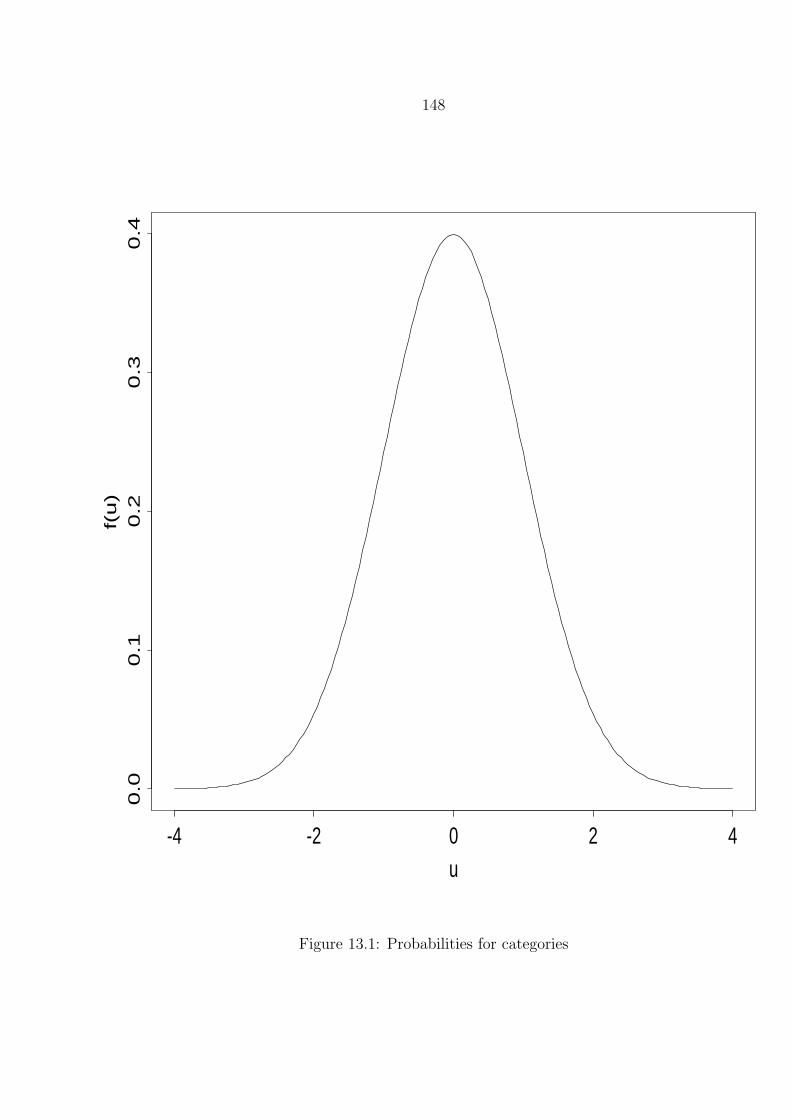
148

u

f(u

)

-4 -2 0 2 4

0.0

0.1

0.2

0.3

0.4

Figure 13.1: Probabilities for categories

149

• We can generalize this to m categories

yi =

1 if y∗i < γ1

2 if γ1 < y∗i ≤ γ2

3 if γ2 < y∗i ≤ γ3...m if γm−1 < y∗i

• This gives the probabilities

Pr(yi = 1) = Φ(γ1 − β′xi)

Pr(yi = 2) = Φ(γ2 − β′xi)− Φ(γ1 − β′xi)

Pr(yi = 3) = Φ(γ3 − β′xi)− Φ(γ2 − β′xi)...

Pr(yi = m) = 1− Φ(γm−1 − β′xi)

= Φ(β′xi − γm−1)

• To write down the likelihood let

zij =

1 if yi = j

0 otherwise for j = 1, . . . ,m.

• ThenPr(zij = 1) = Φ(γj − β′xi)− Φ(γj−1 − β′xi)

150

• The likelihood for an individual is

Li =[Φ(γ1 − β′xi)

]zi1[Φ(γ2 − β′xi)− Φ(γ1 − β′xi)

]zi2

· · ·[1− Φ(γm−1 − β′xi)

]zim

= Πmj=1[Φ(γj − β′xi)− Φ(γj−1 − β′xi)

]zij

• The likelihood function for the sample then is

L = Πni=1Π

mj=1[Φ(γj − β′xi)− Φ(γj−1 − β′xi)

]zij

• We compute marginal effects just like for the dichotomous probit model:

∂ Pr(yi = 1)

∂xi= −φ(γ1 − β′xi)β

∂ Pr(yi = 2)

∂xi= (φ(γ1 − β′xi)− φ(γ2 − β′xi))β

∂ Pr(yi = 3)

∂xi= φ(γ2 − β′xi)β

• Applications:

– Fiorina, Retrospective Voting in American National Elections : Whatfactors affect the strength of party identification?

– Krehbiel and Rivers ’88 AJPS : What factors determine a legislator’svotes on paired legislative proposals?

Section 14

Censored Regression• Observation Scheme #4:

yi =

y∗ if y∗i > 00 if y∗i ≤ 0

• Case 1: yi = 0 ⇒ ui < −β′xi.

Pr(ui < −β′xi) = Pr

(ui

σ>β′xi

σ

)= 1− Pr

(ui

σ<β′xi

σ

)– Information content: 1− Φ(β

′xi

σ ).

• Case 2: yi > 0.

– Information content: f(yi|y∗i > 0) · Pr(y∗i > 0)

– What is f(yi|y∗i > 0)?

– By the definition of conditional probability we have

f(yi|y∗i > 0) =f(yi)

Pr(y∗i > 0).

151

152

y

f(y)

-4 -2 0 2 4

0.0

0.1

0.2

0.3

0.4

Figure 14.1: Censoring

153

−4 −2 0 2 4

−4−2

02

46

x

ysta

r

−4 −2 0 2 4

−4−2

02

46

x

y

Figure 14.2: Censoring and OLS

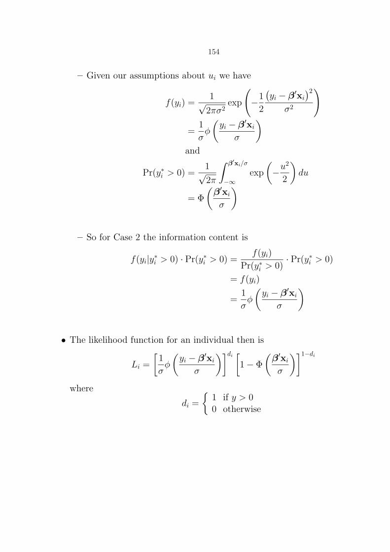
154

– Given our assumptions about ui we have

f(yi) =1√

2πσ2exp

(−1

2

(yi − β′xi

)2σ2

)

=1

σφ

(yi − β′xi

σ

)and

Pr(y∗i > 0) =1√2π

∫ β′xi/σ

−∞exp

(−u

2

2

)du

= Φ

(β′xi

σ

)

– So for Case 2 the information content is

f(yi|y∗i > 0) · Pr(y∗i > 0) =f(yi)

Pr(y∗i > 0)· Pr(y∗i > 0)

= f(yi)

=1

σφ

(yi − β′xi

σ

)

• The likelihood function for an individual then is

Li =

[1

σφ

(yi − β′xi

σ

)]di[1− Φ

(β′xi

σ

)]1−di

where

di =

1 if y > 00 otherwise

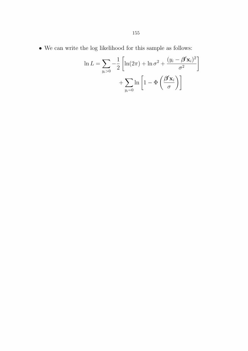
155

• We can write the log likelihood for this sample as follows:

lnL =∑yi>0

−1

2

[ln(2π) + lnσ2 +

(yi − β′xi)2

σ2

]+∑yi=0

ln

[1− Φ

(β′xi

σ

)]

156

14.1 Reparameterization for tobit model

• Let γ = β/σ and θ = 1/σ. The likelihood then becomes

lnL =∑yi>0

−1

2

[ln(2π)− ln θ2 + (θyi − γ ′xi)

2]+∑yi=0

ln [1− Φ (γ ′xi)]

• After estimating this model we can get the parameter estimates of interestback from β = γ/θ and σ = 1/θ.

• We also need the standard errors of β and σ, but we can’t just get them inthe standard way.

• The method that is used is called the delta method; use it to obtain theasymptotic variance-covariance matrix.

• The delta method is used to obtain the asymptotic variance-covariancematrix of a function of a random variable by employing the Taylorapproximation.

157

• For example, suppose we have a sample y1, . . . , yn where the ys are iid withE[yi] = µ and var[yi] = σ2.

• Let y = 1n

∑yi.

• Recall the CLT says:√n(y − µ)

D→ N [0, σ2].

• From the Taylor approximation:

g(y) ≈ g(µ) + g′(µ)(y − µ) + higher order terms

• Rearranging and setting to equal gives

g(y)− g(µ) = g′(µ)(y − µ)

• Multiply through by√n to get

√n(g(y)− g(µ)) = g′(µ)

√n(y − µ)

• By the CLT we know

g′(µ)√n(y − µ)

D→ g′(µ) ·N(0, σ2)D= N(0, (g′(µ))2σ2)

• So √n(g(y)− g(µ))

D→ N(0, (g′(µ))2σ2)

158

• In higher dimensions, this will look like

√n(y − µ)

D→ N [0,Σ]

• So √n(g(y)− g(µ))

D→ N(0,Ω)

where

Ω =∂g(µ)

∂µΣ∂g(µ)

∂µ′

where g(µ) is a set of p continuous functions.

• Using this method for the reparameterized tobit model will give

Asy. var[β, σ2

]= JVJ′

where V is the negative inverse of the estimated Hessian and

J =

[∂β∂γ′

∂β∂θ

∂σ∂γ′

∂σ∂θ

]=

[1θI

−1θ2 γ

0′ −1θ2

]

159

14.2 Marginal Effects

We can compute marginal effects by taking derivatives—but what we take thederivative of depends on the question of interest. Some possibilities are:

• If interested in the marginal effect on the latent variable y∗ do:

∂E[y∗i |xi]

∂xi= β

• If interested in the marginal effect on y, taking into account the censoring:

E[yi|xi] = 0 · Pr(yi = 0|xi) + E[yi|yi > 0,xi] · Pr(y > 0|xi)

=(1− Φ(−β′xi/σ)

) (β′xi + E[ui|ui > −β′xi]

)=(1− Φ(−β′xi/σ)

)(β′xi + σ

φ(β′xi/σ)

Φ(β′xi/σ)

)

Taking the derivative gives

∂E[yi|xi]

∂xi= βΦ

(β′xi

σ

)• If interested in the marginal effect on probability that y exceeds threshold:

∂ Pr[yi > 0|xi]

∂xi= βφ

(β′xi

σ

)

160

−2 −1 0 1 2

0.0

0.5

1.0

1.5

2.0

Marginal effect on y, taking into account the censoring

x

βΦ(βx σ)Φ(βx σ)

−2 −1 0 1 2

0.0

0.2

0.4

0.6

0.8

Marginal effect on probability that y exceeds threshold

x

βφ(βx σ)φ(βx σ)

Figure 14.3: Marginal Effects and Censoring

161

14.3 Heteroskedasticity and the tobit model

• In the presence of heteroskedasticity, the tobit MLE is inconsistent, withthe severity of the inconsistency dependent in part on the number of limitobservations.

• Heteroskedasticity can be handled in the same way as with the probitmodel—i.e., specify the form of the heteroskedasticity such as

σ2i = σ2 exp(ψ′wi)

and then estimate the model. Use LR tests to determine whetherheteroskedastic model is correct.

Section 15

Truncated Regression• Observation Scheme #5:

yi =

y∗ if y∗i > 0? if y∗i ≤ 0

• Case 1: yi > 0.

– Information content:

f(yi|y∗i > 0) =

1σφ(

yi−β′xi

σ

)Pr(y∗i > 0)

• Case 2: yi =?

– Information content: Nada.

• The individual’s contribution to the likelihood function then is

Li =

1σφ(

yi−β′xi

σ

)1− Φ(−β′xi/σ)

• The log-likelihood then is

lnL = −n2

[ln(2π) + lnσ2]− 1

2σ2

n∑i=1

(yi − β′xi)2

−n∑

i=1

ln

[1− Φ

(−β′xi

σ

)]

162

163

• The same reparameterization that was recommended for the tobit model isalso recommended here.

164

15.1 Marginal Effects

• From the moments of the truncated normal we know:

E[yi|yi > 0,xi] =

(β′xi + σ

φ(−β′xi/σ)

1− Φ(−β′xi/σ)

)= β′xi + σλ(αi)

where αi = β′xi/σ and λ(·) = φ(·)/[1− Φ(·)].

∂E[yi|yi > 0,xi]

∂xi= β +

(dλi

dαi

)∂αi

∂xi

= β + σ

(λ2

i − αiλi

(−xi

σ

))= β(1− λ2

i + αiλi)

= β(1− δ(αi))

• Note that 0 < δ(αi) < 1 which implies that truncation leads to anattenuation of the marginal effect that we would see in a linear regression.

Section 16

Sample and Self-Selection Models

• Consider the following research questions:

1. How do certain firm characteristics affect the dollar amount of

fines the firm pays for violating environmental regulations?

2. What factors affect the vote share of incumbents, taking into

account that they have to decide whether or not to run for

reelection?

3. What factors affect the number of troops that a country

commits to a U.N. peacekeeping mission?

• While these questions look similar to the questions for which we

would use truncated or censored regression models, they differ in a

key way.

• While the dependent variable in each of these cases is continuous,

we will only get to observe this dependent variable for certain

outcomes of a stochastic process.

– The kind of sample we get is determined by a stochastic

selection process.

• Another way to think about this is that the truncation points here

may be more appropriately thought of as random rather than

constant.

165

166

• There is some prior decision that we need to account for:

– In Case 1, our sample is determined by an agency’s decisions to

investigate firms.

– In Case 2, our sample is determined by members’ decisions to

seek reelection or retire.

– In Case 3, our sample is determined by countries’ decisions to

participate in the peacekeeping mission.

• These are examples where sample selection models would be

appropriate.

• To answer these questions, we use an empirical model that consists

of more than one equation.

167

• A Model:

Latent structure:

y∗1i = β′1x1i + u1i

y∗2i = β′2x2i + u2i

Observed structure:

y1i =

1 if y∗1i > 0

0 if y∗1i ≤ 0y2i =

y∗2i if y1i = 1

? otherwise

• Assume distribution for us:[u1i

u2i

]∼ N

(0,

[σ2

1 σ12

σ12 σ22

])• That is, we assume that (u1i, u2i) have a bivariate normal

distribution:

f (u1i, u2i) =1

2πσ1σ2

√1− ρ2

× exp

− 1

2(1− ρ2)

[(u1i

σ1

)2

− 2ρu1iu2i

σ1σ2+

(u2i

σ2

)2]

where ρ = σ12σ1σ2

.

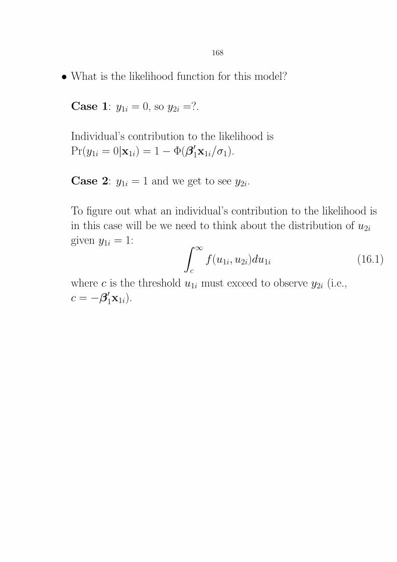
168

• What is the likelihood function for this model?

Case 1: y1i = 0, so y2i =?.

Individual’s contribution to the likelihood is

Pr(y1i = 0|x1i) = 1− Φ(β′1x1i/σ1).

Case 2: y1i = 1 and we get to see y2i.

To figure out what an individual’s contribution to the likelihood is

in this case will be we need to think about the distribution of u2i

given y1i = 1: ∫ ∞

c

f (u1i, u2i)du1i (16.1)

where c is the threshold u1i must exceed to observe y2i (i.e.,

c = −β′1x1i).

169

Trick: a joint distribution can be written as a conditional

distribution times a marginal distribution:

f (u1i, u2i) = f (u2i)f (u1i|u2i).

Then (16.1) can be written as∫ ∞

c

f (u1i, u2i)du1i =

∫ ∞

c

f (u2i)f (u1i|u2i)du1i

= f (u2i)

∫ ∞

c

f (u1i|u2i)du1i

= f (u2i) Pr(u1i > c|u2i)

Given our assumptions, u1i|u2i ∼ N(σ12σ2

2u2i, (1− ρ2)σ2

1

).

What is Pr(u1i > c|u2i)?

u1i − σ12σ2

2u2i

(1− ρ2)1/2σ1>

c− σ12σ2

2u2i

(1− ρ2)1/2σ1

Let c = −β′1x1i and u2i = y2i − β′2x2i. Then

c− σ12σ2

2u2i

(1− ρ2)1/2σ1=−β′1x1i − σ12

σ22(y2i − β′2x2i)

(1− ρ2)1/2σ1

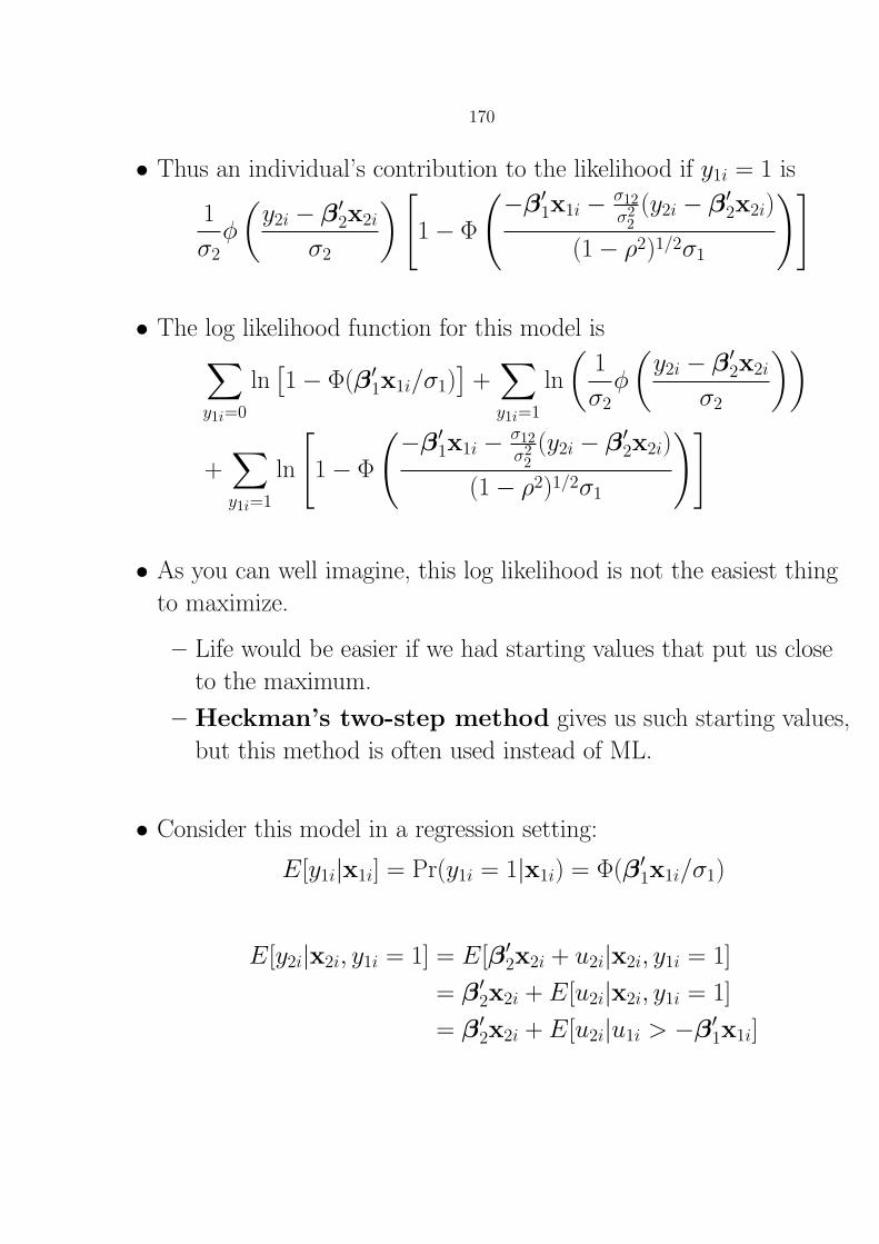
170

• Thus an individual’s contribution to the likelihood if y1i = 1 is

1

σ2φ

(y2i − β′2x2i

σ2

)[1− Φ

(−β′1x1i − σ12σ2

2(y2i − β′2x2i)

(1− ρ2)1/2σ1

)]

• The log likelihood function for this model is∑y1i=0

ln[1− Φ(β′1x1i/σ1)

]+∑y1i=1

ln

(1

σ2φ

(y2i − β′2x2i

σ2

))

+∑y1i=1

ln

[1− Φ

(−β′1x1i − σ12σ2

2(y2i − β′2x2i)

(1− ρ2)1/2σ1

)]

• As you can well imagine, this log likelihood is not the easiest thing

to maximize.

– Life would be easier if we had starting values that put us close

to the maximum.

– Heckman’s two-step method gives us such starting values,

but this method is often used instead of ML.

• Consider this model in a regression setting:

E[y1i|x1i] = Pr(y1i = 1|x1i) = Φ(β′1x1i/σ1)

E[y2i|x2i, y1i = 1] = E[β′2x2i + u2i|x2i, y1i = 1]

= β′2x2i + E[u2i|x2i, y1i = 1]

= β′2x2i + E[u2i|u1i > −β′1x1i]

171

• How might this be problematic for using OLS?

– if E[u2i|u1i > −β′1x1i] = 0, no bias.

– if E[u2i|u1i > −β′1x1i] = a where a is any nonzero constant,

then we get bias in the intercept but not the slope coefficients.

– if E[u2i|u1i > −β′1x1i] = f (β′2x2i), then we get inconsistency in

the intercept and the slope coefficients.

• We can use the law of iterated expectations to figure out

what E[u2i|u1i > −β′1x1i] is.

• Simple version of the law of iterated expectations (from

Wooldridge’s Econometric Analysis of Cross Section and Panel

Data, p. 29):

E[y] = Ex[E[y|x]].

• Think of x as a discrete vector taking on possible values

c1, c2, . . . , cM , with probabilities p1, p2, . . . , pM . Then the LIE says:

E[y] = p1E[y|x = c1] + p2E[y|x = c2] + · · · + pME[y|x = cM ]

• That is, E[y] is simply a weighted average of the E[y|x = cj],

where the weight pj is the probability that x takes on the value of

cj. In other words, a weighted average of averages.

• E.g., suppose we are interested in average IQ generally, but we have

measures of average IQ by gender. We could figure out the quantity

of interest by weighting average IQ by the relative proportions of

men and women.

172

• For our problem:

E[u2i|u1i > −β′1x1i] = Eu1

E[u2i|u1i > −β′1x1i, u1i]|u1i > −β′1x1i]

• Take the inner expectation:

E[u2i|u1i > −β′1x1i, u1i] = E[u2i|u1i]

= τu1i

where

τ =cov(u1i, u2i)

var(u1i)=σ12

σ21

• The outer expectation then becomes

E[τu1i|u1i > −β′1x1i] = τE[u1i|u1i > −β′1x1i]

= τσ1E

[u1i

σ1|u1i

σ1>−β′1x1i

σ1

]= ρσ2

φ(β′1x1i/σ1)

Φ(β′1x1i/σ1)

173

• Putting this altogether gives

E[y2i|x2i, y1i = 1] = β′2x2i + ρσ2φ(β′1x1i/σ1)

Φ(β′1x1i/σ1)

= β′2x2i + βλλ(αi)

where αi = β′1x1i/σ1, λ(·) = φ(·)/Φ(·), and ρσ2 = βλ.

• Why exactly is estimating outcome equation by OLS a bad idea?

1. We have an ommitted variables problem.

2. λ(αi) is a function of x1i and so will be correlated with x1i. If

any elements of x1i are correlated with elements of x2i, the OLS

estimator will be inconsistent.

• Identification issue: what if x1 = x2?

174

• This derivation provides the basis for Heckman’s two-step method.

Step 1: Take full sample and estimate y1 equation by probit.

Step 1.5: Using the (consistent) estimates from this equation,

construct λ = λ(β′1x1i) for selected subsample where y1i = 1.

Step 2: In selected sample, regress y2i onto x2i and λ to obtain

estimates of β2 and βλ.

• Unfortunately, we are not done after Step 2.

• It’s smart to test whether or not sample selectivity exists. We can

do this using the regression in Step 2.

– Null hypotheses: H0 : τ = 0.

– Under this null, τse(τ)

a∼ N(0, 1).

If we fail to reject H0, then we can just use OLS.

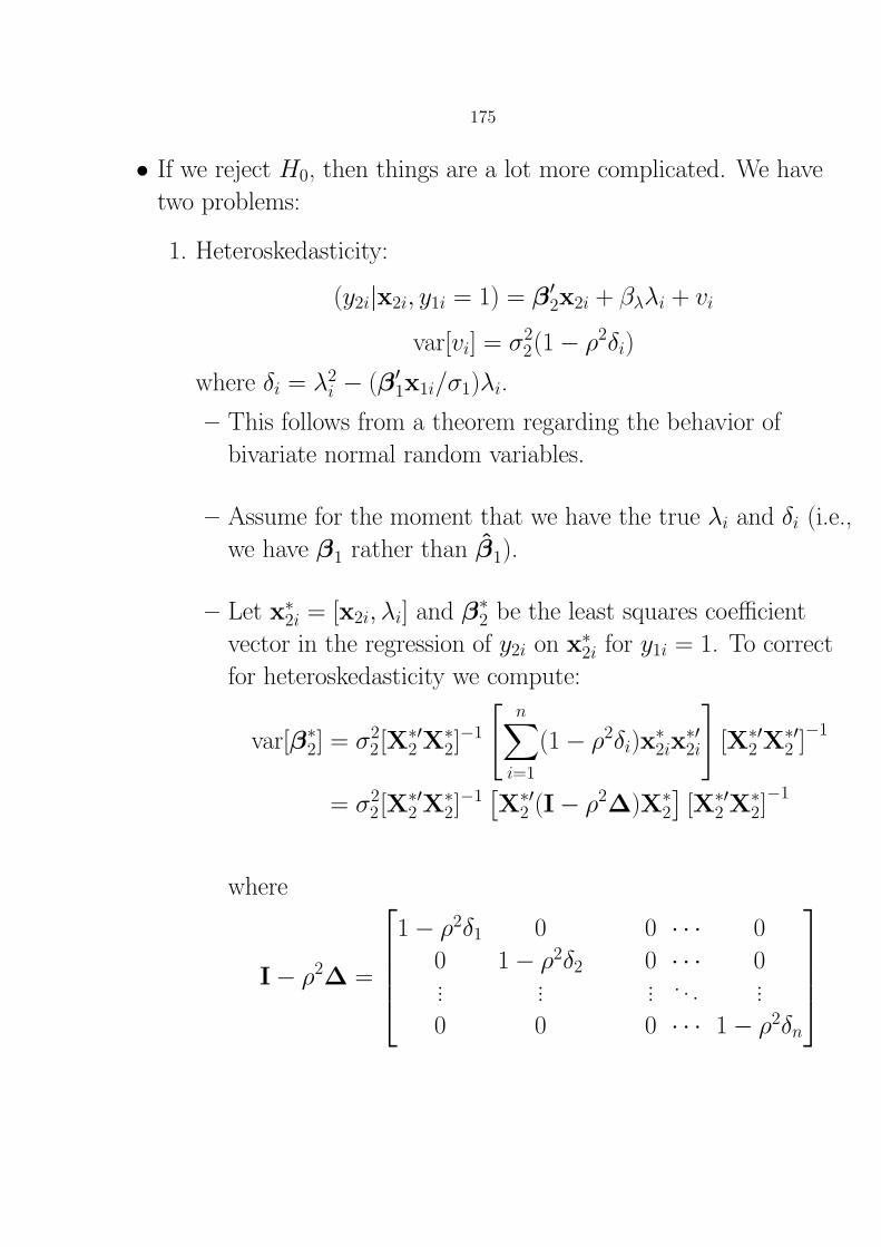
175

• If we reject H0, then things are a lot more complicated. We have

two problems:

1. Heteroskedasticity:

(y2i|x2i, y1i = 1) = β′2x2i + βλλi + vi

var[vi] = σ22(1− ρ2δi)

where δi = λ2i − (β′1x1i/σ1)λi.

– This follows from a theorem regarding the behavior of

bivariate normal random variables.

– Assume for the moment that we have the true λi and δi (i.e.,

we have β1 rather than β1).

– Let x∗2i = [x2i, λi] and β∗2 be the least squares coefficient

vector in the regression of y2i on x∗2i for y1i = 1. To correct

for heteroskedasticity we compute:

var[β∗2] = σ22[X

∗′2 X∗

2]−1

[n∑i=1

(1− ρ2δi)x∗2ix

∗′2i

][X∗′

2 X∗′2 ]−1

= σ22[X

∗′2 X∗

2]−1[X∗′

2 (I− ρ2∆)X∗2

][X∗′

2 X∗2]−1

where

I− ρ2∆ =

1− ρ2δ1 0 0 · · · 0

0 1− ρ2δ2 0 · · · 0... ... ... . . . ...

0 0 0 · · · 1− ρ2δn

176

2. Unfortunately, instead of β1 we have β1 which implies that we

are really estimating

(y2i|x2i, y1i = 1) = β′2x2i + βλλi + εi

where

εi = vi + βλ(λi − λi)

– Since in finite samples β1 6= β1, then λi 6= λi. This implies

there is correlation across observations because the

“measurement error” in estimating β1 is common to all

individuals in the subsample.

– To correct for this problem we compute

var[β2, βλ] = σ22[X

∗′2 X∗

2]−1[X∗′

2 (I− ρ2∆)X∗2 + Q

][X∗′

2 X∗2]−1

where

Q = ρ2(X∗′2 ∆X1)Est. Var[β1](X

′1∆X∗

2)

177

Part V

Probabilistic Choice Models

Section 17

Introduction

• The next set of models we’ll focus on are based on the logistic distri-

bution rather than the normal.

• To fix ideas, consider the binary logit model.

y∗i = β′xi + ui

• Instead of assuming ui follows a normal distribution, we assume it

follows a logistic distribution w/ mean 0 and variance π2/3.

• Going through derivations that are similar to what we did with the

probit model we end up with

Pr(yi = 1) =exp(β′x)

1 + exp(β′x)

• The likelihood function for the logit model then is

L = Πni=1

[exp(β′x)

1 + exp(β′x)

]yi [ 1

1 + exp(β′x)

]1−yi

• We also use models based on the logistic distribution when we have

dependent variables that are categorical and the categories are un-

ordered. For example:

– Transportation choices: bus, car, train.

– Voting choices in elections with more than two candidates.

– Occupational categories: craft, blue collar, white collar, profes-

sional.

178

Section 18

The Multinomial Logit Model

• The set-up:

– n decision makers indexed by i

– J alternatives: 1, 2, . . . , J .

– We observe yi = j if i chooses alternative j.

– We observe a vector of characteristics zi for each i.

– The object of interest is Pij = Pr(yi = j|zi).

• We know Pijε[0, 1], so we want Pij to be proportional to some func-

tion that is nonnegative:

Pij ∝ exp(γ ′jzi)

• The probabilities across choices must sum to one so

J∑j=1

Pij = 1 ⇒ Pij =exp(γ ′jzi)∑Jk=1 exp(γ ′kzi)

179

180

18.1 Identification Issue

• Unknown parameters in model are γ1, γ2, . . . , γJ , but can’t estimate

all of these parameters.

• With J alternatives, if know the choice probabilities for J−1 of these

alternatives, then know the probability of choosing the remaining

alternative.

• Don’t have J independent pieces of information regarding the choice

probabilities.

• ⇒ there can’t be J separate parameter vectors to estimate—only

have J − 1 identifiable parameter vectors.

181

18.2 Normalization

• We need some parameter restrictions to knock out one of the proba-

bilities as an unknown piece of information:

Pij =exp(γ ′jzi)/ exp(γ ′1zi)∑Jk=1 exp(γ ′kzi)/ exp(γ ′1zi)

=exp([γ ′j − γ ′1]zi

)[exp(γ ′1zi) + exp(γ ′2zi) + . . . + exp(γ ′Jzi)] / exp(γ ′1zi)

=exp([γ ′j − γ ′1]zi

)1 +

∑Jk=2 exp ([γ ′k − γ ′1]zi)

=exp(γ ′jzi

)1 +

∑Jk=2 exp (γ ′kzi)

where γ ′j = γ ′j − γ ′1 for j = 2, 3, . . . , J .

• To write down the likelihood function, first define a set of dummy

variables, dij, where

dij =

1 if yi = j

0 otherwise

• The likelihood function for an individual then is

Li = P di1i1 P

di2i2 · · ·P diJ

iJ

=

J∏j=1

Pdij

ij

• The log likelihood for the sample is

lnL =

n∑i=1

J∑j=1

dij lnPij (18.1)

182

• Interpretation of the coefficients in this model is tricky:

∂Pj∂zi

= Pj

[γj −

J∑k=1

Pkγk

]

• Another way to interpret effects is to compute log-odds ratios:

PjPk

=exp(γ ′jzi)/

(1 +

∑Jk=2 exp(γ ′kzi)

)exp(γ ′kzi)/

(1 +

∑Jk=2 exp(γ ′kzi)

)=

exp(γ ′jzi)

exp(γ ′kzi)= exp

([γ ′j − γ ′k]zi

)

183

• Taking logs gives

ln

(PjPk

)= [γ ′j − γ ′k]zi

• Interpretation: we are taking a base case and comparing the proba-

bility of making other choices relative to the base case.

• Consider category 1, where γ1 = 0:

ln

(PjP1

)= γ ′jzi

• So γj gives you the change in the log odds of being in category j

instead of category 1.

Section 19

The Conditional Logit Model

• The conditional logit model is derived from random utility models.

• Key difference between the MNL model and the conditional logit

model: the latter considers the effects of the choice characteristics on

the determinants of choice probabilities.

• Suppose an individual i can choose from J alternatives, we can write

down the utility of choice j as

Uij = β′xij + εij

• We assume that if i chooses j then the utility associated with al-

ternative j is the largest of the utilities obtained from the various

choices. So we are interested in

Pr(Uij > Uik) for k 6= j

• For example,

Pr(yi = 1) = Pr(Ui1 > Ui2)

= Pr(β′xi1 + εi1 > β′xi2 + εi2)

= Pr(εi1 − εi2 > β′xi2 − β′xi1)

184

185

• To derive the statistical model, we make some distributional assump-

tions about εij. Specifically, we assume it has an extreme value dis-

tribution:

F (εij) = exp(− exp(−εij))f (εij) = exp(−εij) exp(− exp(−εij))

• Key things to note:

1. We assume that the εij are iid. This is a very strong assump-

tion: not only are they iid across decision makers, but iid across

alternatives for each decision-maker.

2. We have common parameters across choices. Still have to nor-

malize, though.

• Let Yi indicate the choice of an individual. Then given our assump-

tions, we obtain the conditional logit model as

Pr(Yi = j) =exp(β′xij)∑Jk=1 exp(β′xik)

• The log likelihood for this model has the same form as the log likeli-

hood for the MNL model (i.e., see eq. 18.1).

186

−4 −2 0 2 4 6

0.0

0.1

0.2

0.3

ε

f(ε)

−4 −2 0 2 4 6

0.0

0.2

0.4

0.6

0.8

1.0

ε

F(ε)

Figure 19.1: PDF and CDF for Extreme Value Distribution

187

19.1 Equivalence of the MNL model and conditional logit

model

• It is important to note that the MNL model and conditional logit

model are algebraically equivalent. To see this let

γ ′2 =(0 β 0

)γ ′1 =

(β 0 0

)zi =

xi1xi2xi3

• Then

P2

P1= exp

((0 β 0)−(β 0 0

))xi1xi2xi3

= exp

(−β β 0)xi1

xi2xi3

= exp [β(xi2 − xi1)]

• We could combine the MNL and conditional logit models to get some-

thing like

Pij =exp(β′xij + γ ′jzi)∑Jk=1 exp(β′xik + γ ′kzi)

188

19.2 Independence of Irrelevant Alternatives

• The multinomial logit model has the property known as indepen-

dence of irrelevant alternatives which follows from the iid as-

sumption for the disturbances.

• From above

ln

(PjPk

)= [γ ′j − γ ′k]zi

• This means that the odds ratio between any two choices does not

depend on the other choices. This can be problematic. To see why

consider the classic “red bus, blue bus” problem.

• Suppose individuals have 2 modes of transportation they can choose

from:

1. Car.

2. Red bus.

• Assume individuals are indifferent between traveling by car and by

bus. This implies

Pr(car) = Pr(red bus) = 1/2.

• The odds of taking the car v. the red bus:

Pr(car)/Pr(red bus) = 1.

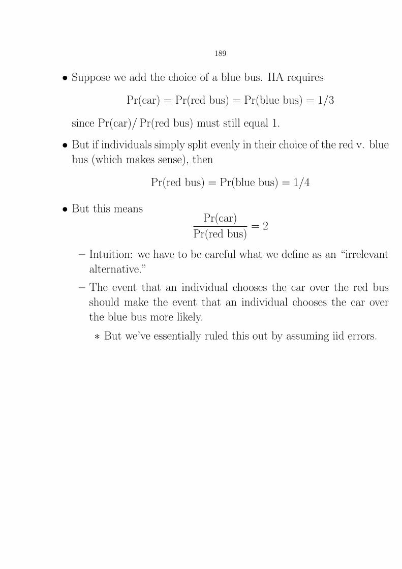
189

• Suppose we add the choice of a blue bus. IIA requires

Pr(car) = Pr(red bus) = Pr(blue bus) = 1/3

since Pr(car)/Pr(red bus) must still equal 1.

• But if individuals simply split evenly in their choice of the red v. blue

bus (which makes sense), then

Pr(red bus) = Pr(blue bus) = 1/4

• But this meansPr(car)

Pr(red bus)= 2

– Intuition: we have to be careful what we define as an “irrelevant

alternative.”

– The event that an individual chooses the car over the red bus

should make the event that an individual chooses the car over

the blue bus more likely.

∗ But we’ve essentially ruled this out by assuming iid errors.

190

• The IIA assumption renders the MNL model highly problematic for

many settings in the social sciences.

• For example:

– Suppose a country has a liberal and conservative party, and a

new conservative party enters.

– IIA ⇒ entrance of the 2nd conservative party should not affect

the relative probability of an individual choosing b/t the liberal

party and the first conservative party.

– Not likely if voters view the two conservative parties as similar.

191

19.3 IIA test

• Intuition: if IIA holds, then you can estimate the model leaving out

one of the alternatives and the coefficient estimates will not change

significantly.

• If you estimate the model excluding an irrelevant alternative then

the parameter estimates will be consistent, but not efficient.

• But if the relative odds ratios between the choices that remain are

not truly independent, then we will get inconsistent estimates after

we eliminate the choice.

• To perform this test we compute the statistic

χ2k =

(βs − βf

)′ [Vs − Vf

]−1 (βs − βf

)where s indicates the estimator using the subset of alternatives, f

indicates the estimator using the full set of alternatives, and Vs and

Vf are the respective asymptotic covariance matrices (k = number

of rows in βs).

• Note that if Vs − Vf is not positive semidefinite, the statistic we

compute can be negative. This is usually taken as evidence that IIA

holds.

• Test is generally of low power.

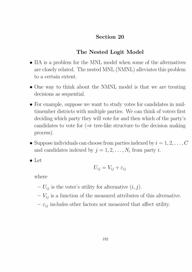
Section 20

The Nested Logit Model

• IIA is a problem for the MNL model when some of the alternatives

are closely related. The nested MNL (NMNL) alleviates this problem

to a certain extent.

• One way to think about the NMNL model is that we are treating

decisions as sequential.

• For example, suppose we want to study votes for candidates in mul-

timember districts with multiple parties. We can think of voters first

deciding which party they will vote for and then which of the party’s

candidates to vote for (⇒ tree-like structure to the decision making

process).

• Suppose individuals can choose from parties indexed by i = 1, 2, . . . , C

and candidates indexed by j = 1, 2, . . . , Ni from party i.

• Let

Uij = Vij + εij

where

– Uij is the voter’s utility for alternative (i, j).

– Vij is a function of the measured attributes of this alternative.

– εij includes other factors not measured that affect utility.

192

193

• If we assume εij has an extreme value distribution then the proba-

bility Pij that the (i, j)th alternative will be chosen is given by

Pij =exp(Vij)∑C

m=1

∑Nmn=1 exp(Vmn)

• Let

Vij = β′xij + γ ′zi

where xij is a vector of variables that vary with both party and

candidates and zi is a vector of variables that vary only with the

party.

• We can write Pij as Pj|i · Pi where

Pj|i =exp(Vij)∑Nik=1 exp(Vik)

=exp(γ ′zi) exp(β′xij)

exp(γ ′zi)∑Ni

k=1 exp(β′xik)=

exp(β′xij)∑Nik=1 exp(β′xik)

and

Pi =

∑Nij=1 exp(Vij)∑C

m=1

∑Nmn=1 exp(Vmn)

=exp(γ ′zi)

∑Nij=1 exp(β′xij)∑C

m=1 exp(γ ′zm)∑Nm

n=1 exp(β′xmn)

• Next, define an inclusive value for the ith choice:

Ii = ln

Ni∑j=1

exp(β′xij)

194

• Then the above equations become

Pj|i =exp(β′xij)

exp(Ii)

Pi =exp(γ ′zi + Ii)∑C

m=1 exp(γ ′zm + Im)

• We can rewrite Pi as

Pi =exp(γ ′zi + τiIi)∑C

m=1 exp(γ ′zm + τiIm)

where τi is a parameter that we will estimate. Note that above we

restricted τi = 1. If we let τ vary then we have the nested logit

model.

• To estimate this model we can use a 2-stage procedure:

1. Estimate β in Pj|i by doing conditional logit.

2. Compute the inclusive values using the estimates of β for all i

categories. Estimate γ and τ by conditional logit.

• As with Heckman’s two step method for selection models, we need

to correct the standard errors from the second stage.

• Another alternative would be to just do full information maximum

likelihood, which involves maximizing the log-likelihood

lnL =∑n

ln(Pj|i · Pi

)• Note that this model can be generalized to more choice-levels.

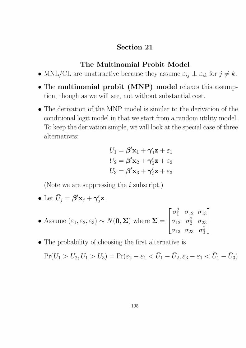
Section 21

The Multinomial Probit Model

• MNL/CL are unattractive because they assume εij ⊥ εik for j 6= k.

• The multinomial probit (MNP) model relaxes this assump-

tion, though as we will see, not without substantial cost.

• The derivation of the MNP model is similar to the derivation of the

conditional logit model in that we start from a random utility model.

To keep the derivation simple, we will look at the special case of three

alternatives:

U1 = β′x1 + γ ′1z + ε1

U2 = β′x2 + γ ′2z + ε2

U3 = β′x3 + γ ′3z + ε3

(Note we are suppressing the i subscript.)

• Let Uj = β′xj + γ ′jz.

• Assume (ε1, ε2, ε3) ∼ N(0,Σ) where Σ =

σ21 σ12 σ13

σ12 σ22 σ23

σ13 σ23 σ23

• The probability of choosing the first alternative is

Pr(U1 > U2, U1 > U3) = Pr(ε2 − ε1 < U1 − U2, ε3 − ε1 < U1 − U3)

195

196

• Let η21 = ε2−ε1 and η31 = ε3−ε1. Then η21 and η31 have a bivariate

normal distribution with covariance matrix

Ω1 =

[σ2

1 + σ22 − 2σ12 σ2

1 − σ13 − σ12 + σ23

σ21 − σ13 − σ12 + σ23 σ2

1 + σ23 − 2σ13

]• Then the probability of choosing category 1 is

P1 =

∫ U1−U2

−∞

∫ U1−U3

−∞f (η21, η31)dη31, dη21

• The probabilities for the other categories are defined similarly.

• The likelihood function for the MNP model looks the same as the

likelihood function for the MNL and conditional logit models.

• Traditionally, the main barrier to using the MNP model has been its

computational difficulty.

• Some advances have been made recently using simulation methods,

but there is still not much progress beyond 3 categories (at least in

political science).

• Fundamental identification issues remain.

197

21.1 Identification of variance-covariance matrix

• Not all of the parameters in Σ can be estimated.

• For the model written in utility differences, it was traditionally thought

that J(J − 1)/2 free parameters could be estimated. More recent

treatments claim that it is possible to estimate only J(J − 1)/2− 1

elements. So need to make assumptions about restrictions.

• Easy way to test if you’ve got an identification problem: nonsensical

parameters or parameters on the boundary.

• A standard assumption is σ2j = 1 ∀ j (i.e., homoskedasticity across

choices).

198

21.2 Application: Alvarez and Nagler “Economics, Issues,

and the Perot Candidacy: Voter Choice in the 1992

Presidential Election” ’95 AJPS

• Key question of concern: how did the candidacy of Ross Perot—

a rare serious 3rd party candidate—affect the outcome of the 1992

presidential election

• Did Perot take away votes from Clinton, Bush, or both?

• Obviously, a model that assumes IIA would have difficulty answering

these questions.

• They estimate a 3-choice MNP using Nat’l Election Survey data.

Their model includes both choice-specific and individual-specific char-

acteristics.

• Normalize on the Perot choice, which makes sense given the stated

goals of the study.

• See table for results.

• In a similar study, Lacy and Burden (“The Vote-Stealing and Turnout

Effects of Ross Perot in the 1992 U.S. Presidential Election” ’99

AJPS ) include the choice to vote in the election.

• However, some questions are raised about the model’s identification.

199

200

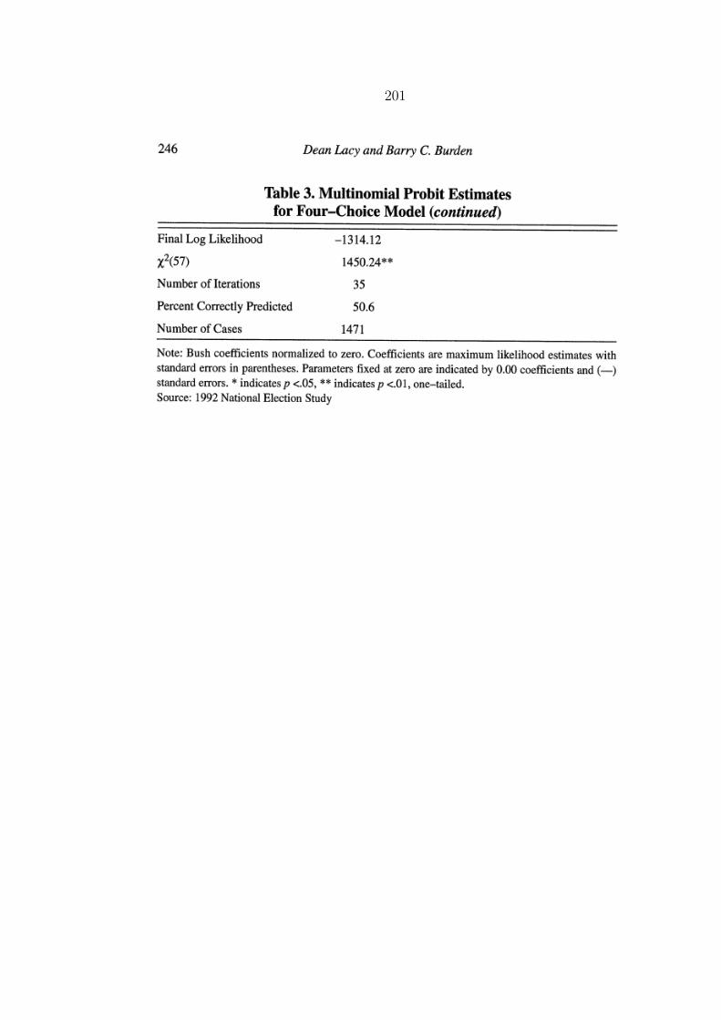
201

202

Part VI

Duration Models

Section 22

Introduction

• These models are used when we are interested in the time it takes

for some event to occur.

• Duration data typically consists of a sample of cross-sections

measured at a set of time intervals: t1, t2, . . . , tK .

• Duration models essentially model the probability of an event

occurring at time t given that the event has not occurred prior to t.

• Censoring: one problem that duration models have to account for is

that the “spells” for some individuals may not end before the

maximum number of time periods is reached.

• Right censoring v. left censoring

• Let T be a continuous random variable with pdf f (t), where t

denotes the realization of T. The probability distribution of the

duration then is

Pr(T < t) = F (t) =

∫ t

0

f (s)ds

203

Section 23

Functions for Analyzing Duration Data

• Given this specification, there are several functions that are useful

for analyzing duration data:

1. The survival function

S(t) = Pr(T ≥ t) = 1− F (t)

which gives the probability that the spell is of length at least t.

2. The hazard rate gives the rate at which spells are completed

at duration t, given that they lasted until t.

λ(t) = lim∆→0

Pr(t ≤ T < t + ∆|T ≥ t)

∆

= lim∆→0

F (t + ∆)− F (t)

∆S(t)

=f (t)

S(t)

3. The integrated hazard function

Λ(t) =

∫ t

0

λ(s)ds

is used in specification tests.

204

205

• The next step is to pick a distribution for F (·). The choice of

distribution depends on what we are trying to model.

• The hazard functions of some popular distributions appear in Table

23. Plots of these hazards appear in Figures 23.1 and 23.2.

Table 23.1: Distributions, Hazard Functions, and Survival Functions

Distribution Hazard Function Survival Function

Exponential λ exp[−λt]

Weibull λp(λt)p−1 exp[−(λt)p]

Lognormal (p/t)φ[p ln(λt)] Φ[−p ln(λt)]

Log-logistic λp(λt)p−1

1+(λt)p1

1+(λt)p

206

Figure 23.1: Plots of hazard functions

1 2 3 4 5 6 7 8

0.10

0.20

0.30

Weibull hazard (lambda=.2)

t

Haz

ard

1.510.5

1 2 3 4 5 6 7 8

0.04

0.08

0.12

0.16

Log−logistic hazard (lambda=.2)

t

Haz

ard

1.510.5

207

Figure 23.2: Lognormal Hazard Function (λ = .5)

5

10

15

20

t

0

0.5

1

1.5

2

p

01

23

4hazard

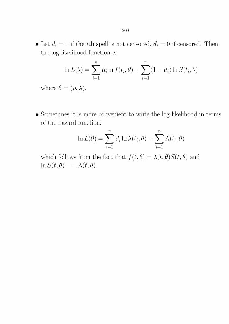
208

• Let di = 1 if the ith spell is not censored, di = 0 if censored. Then

the log-likelihood function is

lnL(θ) =

n∑i=1

di ln f (ti, θ) +

n∑i=1

(1− di) lnS(ti, θ)

where θ = (p, λ).

• Sometimes it is more convenient to write the log-likelihood in terms

of the hazard function:

lnL(θ) =

n∑i=1

di lnλ(ti, θ)−n∑i=1

Λ(ti, θ)

which follows from the fact that f (t, θ) = λ(t, θ)S(t, θ) and

lnS(t, θ) = −Λ(t, θ).

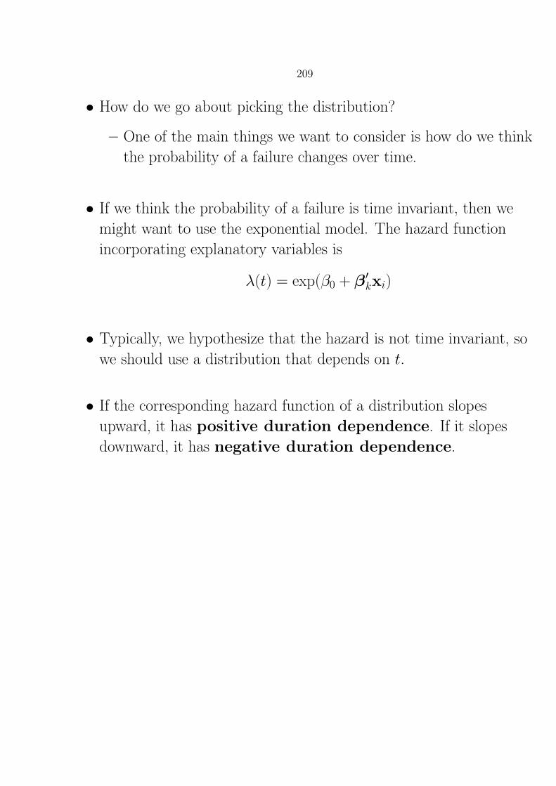
209

• How do we go about picking the distribution?

– One of the main things we want to consider is how do we think

the probability of a failure changes over time.

• If we think the probability of a failure is time invariant, then we

might want to use the exponential model. The hazard function

incorporating explanatory variables is

λ(t) = exp(β0 + β′kxi)

• Typically, we hypothesize that the hazard is not time invariant, so

we should use a distribution that depends on t.

• If the corresponding hazard function of a distribution slopes

upward, it has positive duration dependence. If it slopes

downward, it has negative duration dependence.

210

• The Weibull distribution is popular choice when we want to allow

for time dependence in the model. The hazard function for the

Weibull model with covariates can be specified as

λ(t) = exp(β′xi + α ln t)

This hazard is monotonically increasing or decreasing in t.

• Other distributions allow for more complex time dependencies.

• It is advisable to check whether it is valid to impose this amount of

structure on the data. We can do residual analysis similar to what

we do with OLS.

• The generalized residuals are given by the integrated hazard

function:

ε = Λ(t|θ) = − lnS(t|θ)

• It can be shown that the generalized residuals will follow a unit

exponential distribution. So we can compare the estimated

integrated hazard function against the actual integrated hazard

function for the unit exponential—which is just the 45 degree line.

• If the estimated integrated hazard deviates substantially from this

line, this suggests there is unaccounted for heterogeneity in the data.

211

• Another easy specification check is to split the sample data into

separate groups and estimate the model for each group.

• Greene gives some numerical tests based on conditional moments.

Section 24

Proportional Hazard Model

• The distribution we choose will generally have a substantial impact

on the inferences we make. It would be nice if we had a method

where we didn’t have to specify or parameterize the nature of the

dependence on time.

• One way to do this is the proportional hazard model

developed by Cox. In this model the hazard function depends on a

vector of explanatory variables x with unknown coefficients β and

λ0 that we estimate.

• We factor the hazard function as follows

λ(t,x,β, λ0) = g(x,β)λ0(t)

where λ0(t) is a baseline hazard, corresponding to g(·) = 1.

• The baseline hazard can be chosen from a parametric family and

written as

λ0 = λ0(t, α)

which will give the log-likelihood function

lnL(α,β) =

n∑i=1

di lnλ(ti,xi, α,β)−n∑i=1

Λ(ti,xi, α,β)

• One way to go about estimating this model is to specify λ0(t, α)

and g(·).

212

213

• For the exponential regression specification we choose

g(x,β) = exp(β′x).

and assume λ0(t, α) is constant and normalize it to equal one.

• The log-likelihood function is

lnL(β) =

n∑i=1

diβ′xi −

n∑i=1

ti exp(β′xi)

Section 25

Partial Likelihood Estimator

• We can use the partial likelihood estimator to estimate β

without having to estimate λ0. Suppose we can order the completed

durations as t1 < t2 < . . . < tK and let’s assume there is no

censoring and only one individual exits at each period.

• The conditional probability that one and only one individual exits

at t1 given that any of the individuals could have exited at this time

isλ(t1,x1,β)∑Ki=1 λ(t1,xi,β)

(25.1)

• If we assume λ(t,x,β) = exp(β′x)λ0(t) then (25.1) becomes

exp(β′x1)∑Ki=1 exp(β′xi)

This is the contribution of the shortest duration to the partial

likelihood function.

• The contribution of the jth shortest duration is

exp(β′xj)∑Ki=j exp(β′xi)

214

215

• Things to note:

– With this specification we have taken out the baseline hazard

functions.

– The contribution to the likelihood for each duration is the ratio

of the hazard of the individual whose spell is completed at

duration ti divided by the sum of the hazards of those

individuals who were “at risk” of having their spell completed

at ti.

• The partial log-likelihood then is

lnL =

K∑i=1

β′xi − ln

K∑j=i

exp(β′xj)

• It is a substantial complication to incorporate an exit/failure by

more than one individual at time ti. The general idea is that we

replace xi and xj with the sums of the explanatory variables of the

individuals that fail at each time and account for the different

permutations of failures in the denominator.

• This model can also be altered to account for censoring—see

Lancaster 1990, Ch. 9.

216

• The partial likelihood approach has the following drawbacks:

1. It can perform poorly in small samples relative to the straight

ML approach in terms of the precision of the parameter

estimates.

2. If there are many ties in failure times (> 5% of the sample), can

get bias due to computer programs using an approximation to

the exact partial likelihood.

3. We cannot directly analyze the form of time dependence.

4. It has weaker theoretical foundations than ML.

• Given the drawbacks of the partial likelihood method, we may want

to just choose a distribution for the hazard model and do ML.

Section 26

Nonparametric Approaches

• If we were very concerned about the distortions that parametric

approaches might induce, we could use nonparametric methods.

One such method is the Kaplan-Meier product limit

estimator.

• As with the partial likelihood estimator, we order the completed

durations in our sample from shortest to longest:

t1 < t2 < . . . < tK .

• Define the following terms:

– hj: the number of completed spells of durations tj.

– mj: the number of observations censored between tj and tj+1.

– nj: the number of spells neither completed or censored before

duration tj

nj =

K∑i≥j

(mi + hi)

• The estimator for the hazard function is

λ(tj) =hjnj

217

218

• The estimator for the survival function is

S(tj) =

j∏i=1

(ni − hi)

ni

=

j∏i=1

(1− λi)

• Some other issues:

– Time varying covariates.

– Multiple failure models.

– Competing risk models.

– Split population models.

• Political science applications abound; two notable ones are Katz

and Sala, “Careerism, Committee Assignments, and the Electoral

Connection,” ’96 APSR; and Krehbiel and Kessler, “Dynamics of

Cosponsorship,” ’96 APSR

219

Part VII

Event Count Models

Section 27

Introduction

• Count data is data where the dependent variable assumes

nonnegative integer values (0, 1, 2, . . .) for each of n observations.

These values represent the number of times an event occurs within

a fixed observation period.

• Examples of count data would include number of presidential vetos

per congressional session, annual number of presidential

nominations for the Supreme Court, and the number of military

conflicts between countries.

• Events occur at an unobserved expected rate of event occurrence

during the observation period. We get to see the number of events

that occurred during the period only at the end of the period.

• Least squares regression does not handle these kinds of data very

well:

– The linearity assumption is inappropriate for count data.

– Count data typically come from distributions that are

heteroskedastic. As a result least squares tends to be inefficient

and it gives inconsistent standard errors.

220

Section 28

Poisson Regression Model

• Given these problems, a likelihood approach based on probability

models is attractive. The Poisson regression model has been

popular for analyzing count data.

• For the Poisson model, we assume that the ith event

count—denoted yi—is a draw from a Poisson distribution with

parameter λi.

• To build the likelihood function we start with

Pr(Yi = yi) =exp(−λi)λyii

yi!, yi = 0, 1, 2, . . .

• We model the mean λi as a function of explanatory variables:

ln(λi) = β′xi

• Thus the expected number of events per period is given by

E[yi|xi] = λi = exp(β′xi)

• A feature of the Poisson distribution is that its mean is equal to its

variance. So var[yi|xi] = exp(β′xi) as well.

221

222

• Marginal effects are given by

∂E[yi|xi]∂xi

= λiβ

• The log-likelihood function for the Poisson model is

lnL =

n∑i=1

[−λi + yiβ′xi − ln yi!]

223

28.1 Dispersion

• The derivation of the Poisson model requires the assumption that

the probability of an event occurring at any instant is constant

within a given period and independent of all previous events during

that observation period.

• These assumptions of homogeneity and independence are necessary

if the data generating process is to have the feature of the Poisson

distribution that the E[yi] = var[yi].

• But we may have reason to believe that these assumptions do not

hold.

• Suppose we were counting the number of presidential vetos in a

congressional session.

• If presidents were more likely to veto at certain times during the

session (e.g., near the end of the fiscal year when it is necessary to

pass appropriations bills) or if a successful veto might lead to

President to veto more legislation then the assumptions of

homogeneity and independence would be violated (i.e., there is

heterogeneity and contagion in the data generating process).

224

• If E[yi] 6= var[yi] we will get consistent but inefficient estimates and

inconsistent standard errors.

• Let var[yi] = λiσ2, where σ2 is the dispersion parameter. Then

we have the following possible situations:

Poisson dispersion if σ2 = 1 ⇒ E[yi] = var[yi]

Overdispersion if σ2 > 1 ⇒ E[yi] < var[yi]

Underdispersion if 0 < σ2 < 1 ⇒ E[yi] > var[yi]

• Overdispersion can occur if there is heterogeneity in the data. For

example, certain classes of bills that pass Congress might have a

higher probability of being vetoed than others.

• Positive contagion can also lead to overdispersion. This occurs

when the occurrence of previous events increases the likelihood of

future events.

• Negative contagion—when the number of previous events

decreases the likelihood of future events—induces underdispersion.

Underdispersion is much less common in social science settings.

225

28.2 Tests for Overdispersion

1. Regression-based test: The hypotheses we test are

H0 :var[yi] = E[yi]

H1 :var[yi] = E[yi] + αg(E[yi])

We estimate the regression

zi = δ0 + εi

or

zi = δ1λi + εi

where

zi =(yi − λi)

2 − yi

λi√

2

and λi is the predicted value from the Poisson model. We then do a

t test to see whether δ0 or δ1 is statistically different from zero. If

they are, we reject H0.

226

2. Lagrange Multiplier (LM) test: This test is similar to a

likelihood ratio test (in fact, the two tests are asymptotically

equivalent), except that the LM test requires us to estimate only

the restricted model.

• The intuition behind the LM test is that if the restrictions are

valid then the restricted estimator should be close to the point

that maximizes the likelihood function, which implies that the

slope of the log-likelihood function should be near zero at the

restricted estimator.

• The test is based on the slope of the log-likelihood at the point

where the function is maximized subject to the restriction.

• The restricted model in this case is the Poisson model. The LM

statistic is given by

LM =

∑n

i=1

[(yi − λi)

2 − yi

]√

2∑n

i=1 λi2

2

=(e′e− ny)2

2λ′λ

This follows a chi-squared distribution with the degrees of

freedom equal to the number of restrictions.

Section 29

Gamma Model for Overdispersion

• In the case of overdispersion, our likelihood function will be based

on the negative binomial distribution.

• To account for heterogeneity, we generalize the Poisson model by

assuming that λi is a random variable which follows a gamma

distribution:

fγ(λ|φi, σ2) =λφi/(σ

2−1)−1 exp(−λ/(σ2 − 1))

Γ [φi/(σ2 − 1)] (σ2 − 1)φi/(σ2−1)

where λ, φ, and σ2 are all greater than zero and

Γ(x) =

∫ ∞

0

zx−1 exp(−z)dz

• With this parameterization E(λi) = φ and var(λi) = φ(σ2 − 1).

• We can write the joint distribution of Yi and λ as

f (yi, λi|φi, σ2) = fp(yi|λi)fγ(λi|φi, σ2)

where fp denotes the Poisson distribution.

227

228

• After a rather messy derivation we get the negative binomial

distribution

fnb(yi|λi, σ2) =Γ(

λiσ2−1

+ yi

)Γ(

λiσ2−1

)yi!

(σ2 − 1

σ2

)yi(σ2)

−λiσ2−1

where λi > 0 and σ2 > 1.

• Now E(Yi) = λi and var(Yi) = λiσ2.

• We can include explanatory variables in the same manner as before:

λi = exp(β′xi).

• The log-likelihood function is

lnL =

n∑i=1

ln Γ

(λi

σ2 − 1+ yi

)− ln Γ

(λi

σ2 − 1

)+yi ln(σ2 − 1)− lnσ2

(yi +

λiσ2 − 1

)

Section 30

Binomial Model for Underdispersion

• In the case of underdispersion, our likelihood function is based on a

binomial distribution:

fb(yi|λi, σ2) =Γ(−λiσ2−1

+ 1)

yi!Γ(−λiσ2−1

− yi + 1) (1− σ2

)yi (σ2)−λi

σ2−1−yi

where E(Yi) = λi > 0, var(Yi) = λiσ2 and 0 < σ2 < 1.

• One problem with this distribution is that if −λi/(σ2 − 1) is not an

integer then∞∑m=0

fb(yi|λi, σ2) 6= 1

• This is easily fixed simply by dividing fb(·) by a scaling factor that

assures the probabilities sum to one:

fcpb(yi|λi, σ2) =fb(yi|λi, σ2)

Di

where

Di =

[ −λiσ2−1

)+1∑

m=0

fb(m|λi, σ2)

Note that this imposes a theoretical maximum on the count

variable: −λi/σ2 − 1.

229

230

• The log-likelihood function corresponding to the continuous

parameter binomial distribution is

lnL =

n∑i=1

ln Γ

(−λiσ2 − 1

+ 1

)− ln Γ

(−λiσ2 − 1

− yi + 1

)+ yi ln

(1− σ2

)+

(−λiσ2 − 1

− yi

)ln(σ2)− ln(Di)

• One way to proceed would be to do some sort of pretest that tells

us the type of dispersion and then estimate the appropriate

likelihood function. This has the drawback that if the test is

incorrect, then we can make incorrect inferences.

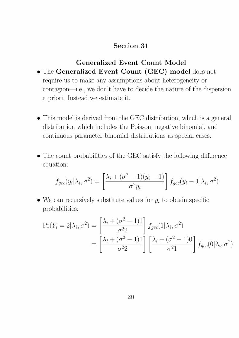
Section 31

Generalized Event Count Model

• The Generalized Event Count (GEC) model does not

require us to make any assumptions about heterogeneity or

contagion—i.e., we don’t have to decide the nature of the dispersion

a priori. Instead we estimate it.

• This model is derived from the GEC distribution, which is a general

distribution which includes the Poisson, negative binomial, and

continuous parameter binomial distributions as special cases.

• The count probabilities of the GEC satisfy the following difference

equation:

fgec(yi|λi, σ2) =

[λi + (σ2 − 1)(yi − 1)

σ2yi

]fgec(yi − 1|λi, σ2)

• We can recursively substitute values for yi to obtain specific

probabilities:

Pr(Yi = 2|λi, σ2) =

[λi + (σ2 − 1)1

σ22

]fgec(1|λi, σ2)

=

[λi + (σ2 − 1)1

σ22

] [λi + (σ2 − 1)0

σ21

]fgec(0|λi, σ2)

231

232

• This generalizes to

fgec(yi|λi, σ2) = fgec(0|λi, σ2)

yi∏j=1

[λi + (σ2 − 1)(j − 1)

σ2j

](31.1)

for yi ∈ 1, 2, 3, . . ..

• In order to get Pr(Yi = 0|λi, σ2) = fgec(0|λi, σ2) we can use the

axiom of probability that

∞∑m=0

fgec(m|λi, σ2) = 1

(i.e., yi takes on some value in a given period with probability 1).

• Summing over both sides of Eq. 31.1 and solving for fgec(0|λi, σ2)

gives

fgec(0|λi, σ2) =

∞∑m=1

m∏j=1

(λi + (σ2 − 1)(j − 1)

σ2j

)−1

• We can then use standard results on the convergence of infinite

series to solve for the probability of zero events. These terms will

vary with the value of σ2:

fgec(0|λi, σ2) =

exp(−λi) for yi = 0 and σ2 = 1

(σ2)−λi/(σ2−1) for yi = 0 and σ2 > 1

(σ2)−λi/(σ2−1)D−1

i for yi = 0 and 0 < σ2 < 1

233

• Collecting all this together gives the following distribution:

fgec(yi|λi, σ2)

=

fgec(0|λi, σ2)∏yi

j=1

[λi+(σ2−1)(j−1)

σ2j

]for yi = 1, 2, . . .

exp(−λi) for yi = 0 and σ2 = 1

(σ2)−λi/(σ2−1) for yi = 0 and σ2 > 1

(σ2)−λi/(σ2−1)D−1

i for yi = 0 and 0 < σ2 < 1

and yi ≤[−λiσ2−1

)+ 1

0 otherwise

• The log-likelihood of for this distribution (reduced to sufficient

statistics) is

lnL(β, σ2) =

n∑i=1

Ci − yi lnσ2 +

yi∑j=1

ln[exp(β′xi) + (σ2 − 1)(j − 1)]

where

Ci =

− exp(β′xi) for σ2 = 1

− exp(β′xi) lnσ2(σ2 − 1)−1 for σ2 > 1

− exp(β′xi) lnσ2(σ2 − 1)−1 − ln(Di) for 0 < σ2 < 1

Section 32

Hurdle Poisson Models

• In some situations, it is unreasonable to assume that the process

generating counts of zero is the same as the one generating positive

outcomes.

• In such cases, we would want to alter standard count models to try

to model these separate processes. Essentially, we want to model

the contributions to the likelihood of the zero observations

differently from the contributions of the positive ones.

• One way to do this is to have a binary probability model that

determines whether a zero or positive outcome occurs and then use

a truncated Poisson distribution for the positive outcomes. For

example:

Pr(Yi = 0) = exp(−θ)

Pr(Yi = yi) =(1− exp(−θ)) exp(−λi)λyii

yi!(1− exp(−λi)), yi = 1, 2, . . .

• Note:

– Probability of non-zero outcomes is rescaled, so that all sum to

1.

– Probability of zero outcomes is not a function of covariates—can

generalize this though.

– Negative binomial version also exists.

234

235

• For a political science perspective on Poisson models see King,

“Statistical Models for Political Science Event Counts” ’88 AJPS.

• For the development of the GEC model see King, “Variance

Specification in Event Count Models: From Restrictive

Assumptions to a Generalized Estimator.” ’89 AJPS.

• For political science applications of event count models see

– Canon, “Sacrificial Lambs or Strategic Politicians: Political

Amateurs in U.S. House Elections.” ’93 AJPS.

– Krause, “Federal Reserve Policy Decision Making.” ’94 AJPS.

– Wang et al. “Inequality and Political Violence Revisited.” ’93

APSR.

236

Part VIII

Models for RepeatedObservations—Dichotomous Dependent

Variables

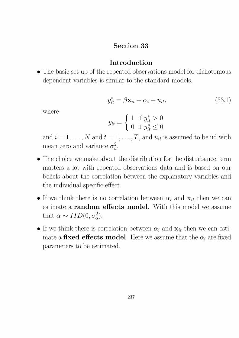
Section 33

Introduction

• The basic set up of the repeated observations model for dichotomous

dependent variables is similar to the standard models.

y∗it = βxit + αi + uit, (33.1)

where

yit =

1 if y∗it > 0

0 if y∗it ≤ 0

and i = 1, . . . , N and t = 1, . . . , T , and uit is assumed to be iid with

mean zero and variance σ2u.

• The choice we make about the distribution for the disturbance term

matters a lot with repeated observations data and is based on our

beliefs about the correlation between the explanatory variables and

the individual specific effect.

• If we think there is no correlation between αi and xit then we can

estimate a random effects model. With this model we assume

that α ∼ IID(0, σ2α).

• If we think there is correlation between αi and xit then we can esti-

mate a fixed effects model. Here we assume that the αi are fixed

parameters to be estimated.

237

238

• If T → ∞, then it is possible to get consistent estimates of β and

αi.

• However, if T is fixed and N → ∞, then we have the incidental

parameters problem—i.e., since the number of parameters increases

with N , we cannot consistently estimate αi for fixed T .

• Unfortunately, the inconsistency in αi is transmitted to β.

• In the linear regression case we take out the individual effect by

subtracting off the means of the variables. That is, if we take the

average over time of eq. 33.1, we get

y∗i = βxi + αi + ui, (33.2)

where y∗i =∑T

t=1 y∗it/T . Subtracting eq. 33.2 from eq. 33.1 gives

y∗it − y∗i = β(xit − xi) + (uit − ui), (33.3)

• But this transformation is not valid with a qualitative limited depen-

dent variable model.

• Such models are nonlinear and so mean-differencing will not work to

remove the individual specific effects.

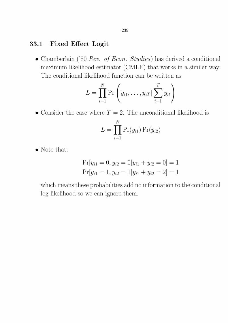
239

33.1 Fixed Effect Logit

• Chamberlain (’80 Rev. of Econ. Studies) has derived a conditional

maximum likelihood estimator (CMLE) that works in a similar way.

The conditional likelihood function can be written as

L =

N∏i=1

Pr

(yi1, . . . , yiT |

T∑t=1

yit

)

• Consider the case where T = 2. The unconditional likelihood is

L =

N∏i=1

Pr(yi1) Pr(yi2)

• Note that:

Pr[yi1 = 0, yi2 = 0|yi1 + yi2 = 0] = 1

Pr[yi1 = 1, yi2 = 1|yi1 + yi2 = 2] = 1

which means these probabilities add no information to the conditional

log likelihood so we can ignore them.

240

• But

Pr[yi1 = 0, yi2 = 1|yi1 + yi2 = 1] =Pr[yi1 = 0, yi2 = 1 and yi1 + yi2 = 1]

Pr[yi1 + yi2 = 1]

=Pr[yi1 = 0, yi2 = 1 and yi1 + yi2 = 1]

Pr[yi1 = 0, yi2 = 1] + Pr[yi1 = 1, yi2 = 0]

• If we assume that the data follow a logistic distribution then we can

rewrite this as

11+exp(αi+β

′xi1)exp(αi+β

′xi2)1+exp(αi+β

′xi2)

11+exp(αi+β

′xi1)exp(αi+β

′xi2)1+exp(αi+β

′xi2)+ exp(αi+β

′xi1)1+exp(αi+β

′xi1)1

1+exp(αi+β′xi2)

which simplifies to

exp(β′xi2)

exp(β′xi1) + exp(β′xi2)

• The expression for the remaining probability is similarly derived.

These probabilities then constitute the conditional log-likelihood func-

tion, which can be maximized using standard techniques.

• This can be extended to T of arbitrary size but the computations are

excessive for T > 10.

241

• Can’t use standard specification test like LR for checking unit het-

erogeneity b/c likelihoods are not comparable (CML uses a restricted

data set).

• But can use this estimator to do a Hausman test for the presence of

individual effects.

• Intuition: in the absence of individual specific effects, both the Cham-

berlain estimator and the standard logit maximum likelihood estima-

tor are consistent, but the former is inefficient. If individual specific

effects exist, then the Chamberlain estimator is consistent while the

standard logit MLE is inconsistent.

– Inefficiency is due to loss of information/throwing away observa-

tions.

• We compute the following statistic for the test:

χ2k =

(βCML − βML

)′[VCML −VML]−1

(βCML − βML

)If we get a significant χ2 value we reject the null of no individual

specific effects.

242

33.2 Random Effects Probit

• The probit model does not lend itself to the fixed effects treatment

because there is no way to sweep out the individual specific effects.

But we can estimate a probit model if we assume random effects.

• Let

εit = αi + uit

and assume αi ∼ N(0, σ2α); uit ∼ N(0, σ2

u), and αi and uit are

independent of each other. Then

var[εit] = σ2u + σ2

α = 1 + σ2α

and

corr[εit, εis] = ρ =σ2α

1 + σ2α

for t 6= s. This implies σ2α = ρ/(1− ρ).

• We can write the probability associated with an observation as

Pr[yit] =

∫ qitβ′xit

−∞f (εit)dεit = Φ[qitβ

′xit]

where qit = 2yit − 1.

• Because of the αi, the T observations for i are jointly normally dis-

tributed. The individual’s contribution to the likelihood is

Li = Pr[yi1, yi2, . . . yiT ]

=

∫ qi1β′xi1

−∞

∫ qi2β′xi2

−∞· · ·∫ qiTβ

′xiT

−∞f (εi1, εi2, . . . , εiT )dεiT · · · εi2εi1

243

• Rather than evaluating multiple integrals, a simplification is possible.

Consider the joint density:

f (εi1, . . . , εiT , αi) = f (εi1, . . . , εiT |αi)f (αi)

• We can then integrate over αi:

f (εi1, . . . , εit) =

∫ ∞

−∞f (εi1, . . . , εiT |αi)f (αi)dαi

• Conditioned on αi, the εis are independent:

f (εi1, . . . , εit) =

∫ ∞

−∞

T∏t=1

f (εit|αi)f (αi)dαi

• Letting ri = αi/(σα√

2) and making the change of variable gives i’s

contribution to the likelihood as

Li =1√π

∫ ∞

−∞e−r

2i

T∏t=1

Φ[qit(β′xit + θri)]

dri (33.4)

θ =

√2ρ

1− ρ(33.5)

244

• Things to note:

– The assumption that the αi and xit are uncorrelated is very re-

strictive. We are also assuming that the within-cross section cor-

relation is the same across all time periods.

– ρ can be interpreted as the proportion of the variance contributed

by the unit effects.

– We can test for unit heterogeneity by checking the statistical

significance of ρ. One way to do this is with a likelihood ratio

ratio test of the random effects probit and pooled probit models.

– The standard way to evaluate the integral in the likelihood is

by Gauss-Hermite quadrature. This raises some concerns about

how the size of T and N affect the accuracy of the quadrature

approximation, and some checks of the performance of the ap-

proximation are in order.

– Stata’s xtprobit command can be used to estimate this model.

– We could derive this model for the logistic distribution rather

than the normal distribution.

245

33.3 Correlated Random Effects Probit

• The big drawback of the random effects model is the unattractive

assumption that the αi and xi are uncorrelated.

• Chamberlain has proposed a correlated random effects (CRE) model

that gets around this problem by assuming a specific functional re-

lationship between αi and xi. That is,

αi =

T∑t=1

a′txit + ηi = a′xi + ηi

where a′ = (a′1, . . . , a′T ), x′i = (x′i1, . . . ,x

′iT ), and ηi is normally

distributed (with mean zero and variance σ2η) and is independent of

the xit.

• The at are vectors of parameters to be estimated and capture the

nature of the relationship between αi and xit.

• Equation (33.1) then becomes

y∗it = β′xit +

T∑t=1

a′txit + εit

where εit = ηi + uit.

246

• Estimation of the CRE model proceeds in a sequential manner:

1. Estimate separate probit equations by maximum likelihood for

each time period, regressing the dependent variable in each period

on all of the leads and lags of the explanatory variables.

2. Stack the estimates from each of these probits into a vector π

and construct the joint covariance matrix of all of the estimates.

The vector π is a vector of reduced form estimates.

3. Use a minimum distance estimator to impose restrictions on π to

back out estimates of the structural parameters β and at. Let

θ = (β′, a′) and choose θ to minimize

[π − f(θ)]′ Ω−1

[π − f(θ)] ,

where Ω is an estimate of the asymptotic variance-covariance

matrix for the reduced-form estimates.

4. We then conduct our standard hypothesis tests to make inferences

about the effects of the variables of interest.

5. Marginal effects can be determined by simulating probabilities:

Pr(yit = 1) = Φ

[(1 + σ2

η)−1/2(β′xit +

T∑t=1

a′txit)

](33.6)

247

• One key advantage of the CRE estimator: allows for an explicit test

for correlation between the individual specific effect and the explana-

tory variables.

• One drawback of the CRE estimator: requires us to impose a good

deal of structure on the relationship between αi and xit and restricts

us to including only time-varying variables in xit.

• Including time invariant variables in xit in effect induces perfect

collinearity since the values of the leads and the lags of these variables

will be the same within each cross-sectional unit.

• Its drawbacks aside, this estimator is part of a class of generalized

method of moments estimators that give substantial efficiency gains

over pooled probit estimators, which ignore individual specific effects.

• For details of the estimation procedure for the CRE model, see

Hsiao’s treatment in Analysis of Panel Data, which is more ac-

cessible than Chamberlain’s original derivation.

• Can be estimated w/ standard software with some more restrictive

assumptions; GAUSS code is available for the general model.

248

33.4 CRE Probit Application: PAC contributions and roll

call votes

• A major concern is the effects of campaign contributions on the be-

havior of members of the U.S. Congress.

• Assessing these effects is complicated because it is methodologically

difficult to account for members’ predispositions to vote in favor of

PACs’ interests.

• CRE probit model can help overcome this problem because it enables

us to account for individual specific effects, such as the predisposition

to vote for or against a particular piece of legislation, which are too

costly or impossible to measure.

• I conducted a CRE probit analysis of roll-call votes and PAC contri-

butions using sets of roll-call votes that are of particular interest to

certain types of PACs (Wawro ’01 AJPS ).

– Tables 3 and 4 report results of the CRE estimation.

– Figures 2 & 4 plot simulated probabilities based on the CRE

estimates.

249

250

251

Section 34

Binary Time-Series Cross-Section (BTSCS) Data

• The methods above are appropriate when N is large and T is small.

Beck, Katz, and Tucker (’98 AJPS ) derive a method for when T is

large.

• The method is based on the observation that BTSCS data is identical

to grouped duration data. That is, we get to observe whether an

event occurred or not only after the end of some discrete period (e.g.,

a year).

• Thus, we can use duration methods to correct for the problem of

temporal dependence.

• Start from the hazard rate for the continuous time Cox proportional

hazard model:

λ(t) = exp(β′xit)λ0(t)

• The survival function is given by

S(t) = exp

(−∫ t

0

λ(τ )dτ

)

252

253

• Assuming we get to observe only whether or not an event occurred

between time tk − 1 and tk, we can write

Pr(yitk = 1

)= 1− exp

(−∫ tk

tk−1

λi(τ )dτ

)= 1− exp

(−∫ tk

tk−1

exp(β′xit)λ0(t)dτ

)= 1− exp

(− exp(β′xit)

∫ tk

tk−1

λ0(t)dτ

)• Let

αtk =

∫ tk

tk−1

λ0(t)dτ

κtk = ln(αtk)

• Then

Pr(yitk = 1

)= 1− exp

(− exp(β′xit)αtk

)= 1− exp

(− exp(β′xit + κtk)

)• This is a binary model with a complimentary log-log (cloglog) link.

The cloglog link is identical to a logit link function when the proba-

bility of an event is small (< 25%) and extremely similar when the

probability of an event is moderate (< 50%).

254

• For ease of application then, Beck, Katz, and Tucker recommend

using the logistic analogue

Pr (yit = 1|xit) =1

1 + exp(−(β′xit + κt−t0))

where κt−t0 is a dummy variable marking the length of the sequence

of zeros that precede the current observation. For example,

t 1 2 3 4 5 6 7 8 9

y 0 0 0 1 0 1 1 0 0

κ κ1 κ2 κ3 κ4 κ1 κ2 κ1 κ1 κ2

• The intuition behind why ordinary logit is inadequate for BTSCS

data is that it doesn’t allow for a nonconstant baseline hazard.

• Including the κ dummies allows duration dependence by allowing for

a time-varying baseline hazard.

• To see how the κ dummies are interpretable as baseline probabilities

or hazards, note

Pr (yit = 1|xit = 0, t0) =1

1 + exp(−κt−t0)

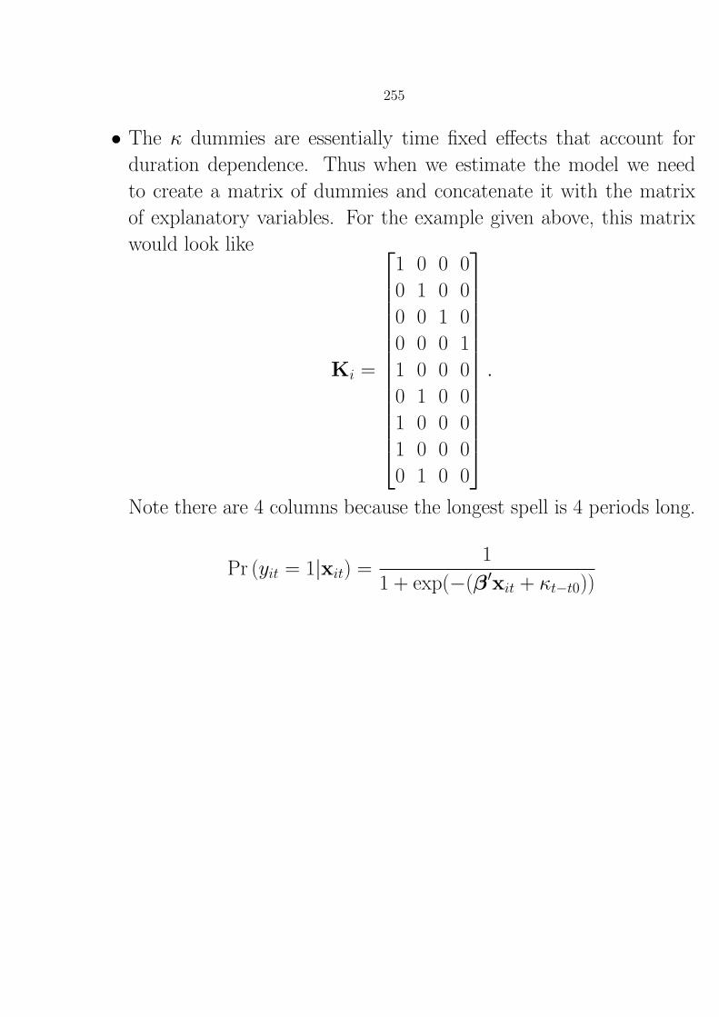
255

• The κ dummies are essentially time fixed effects that account for

duration dependence. Thus when we estimate the model we need

to create a matrix of dummies and concatenate it with the matrix

of explanatory variables. For the example given above, this matrix

would look like

Ki =

1 0 0 0

0 1 0 0

0 0 1 0

0 0 0 1

1 0 0 0

0 1 0 0

1 0 0 0

1 0 0 0

0 1 0 0

.

Note there are 4 columns because the longest spell is 4 periods long.

Pr (yit = 1|xit) =1

1 + exp(−(β′xit + κt−t0))

Section 35

Generalized Estimating Equations (GEEs)

• This class of models allows us to account for unobserved correlation

among observations, without including unit-specific effects.

• GEEs relax assumptions about the independence of observations:

observations are grouped into clusters and then parameters are esti-

mated to model the correlations among observations in the cluster.

• This class of models is derived from the General Linear Model (GLM)

approach.

– Models in which one specifies the “link” function E(Yi) = µi =

h(β′xi) and the relationship between the mean and the variance

(e.g. Vi = g(µi)).

– Standard GLMs obtain estimates by solving the “score equa-

tions”:

Uk(β) =

N∑i=1

DiV−1i (Yi − µi) = 0 (35.1)

where Di = ∂µi∂β and Vi is the variance matrix.

256

257

35.1 GLMs for Correlated Data

• Consider E(Yit) = µit = g(β′xit), T > 1.

• Must make some provision for dependence within i, across t.

• Specify the conditional within-unit or within-cluster correlation:

• Define the “working” T × T correlation matrix Ri(α) as a function

of α.

• Structure (but not the elements) of Ri(α) determined by the inves-

tigator.

• Then redefine the variance matrix in Equation 35.1 as:

Vi =(Ai)

12Ri(α)(Ai)

12

φ(35.2)

where the Ai are T × T diagonal matrices w/ g(µit) along the diag-

onal.

• Intuition:

– Choose β so that µit is “close” to Yit on average,

– Optimally weight each residual (Yit−µit) by the inverse of cov(Yi).

258

35.2 Options for specifying within-cluster correlation

• “Working Independence”: Ri(α) = I

– No within-unit correlation (completely pooling observations).

– Just like standard logit/probit.

• “Exchangeable”: Ri(α) = ρ

– Within-unit correlation is the same across units.

– Similar to “random effects,” in the sense that we’re assuming

constant within-unit marginal covariance; but do not need or-

thogonality assumption of RE.

• Autoregressive : Ri(α) = ρ|t−s|

– Here, AR(1).

– Correlation decays over “time.”

– Can also do “banded” / “stationary” correlations.

• “Unstructured” : Ri(α) = αst, t 6= s

– α is a T × T matrix.

– Allows T (T−1)2 unique pairwise correlations.

– Very flexible, but can be hard to estimate, esp. w/ large T .

259

35.3 “Robust” Standard Errors

• βGEE is robust to misspecification of Ri(α).

• var(βGEE) is not.

• Can compute “sandwich” estimator: var(βGEE) =

N

(N∑i=1

D′iV

−1

i Di

)−1( N∑i=1

D′iV

−1

i SiV−1

i Di

)(N∑i=1

D′iV

−1

i Di

)−1

(35.3)

where Si = (Yi − µi)(Yi − µi)′.

• Similar to the Huber/White estimator.

• One drawback of GEE is that it does not produce standard errors for

elements of Ri(α) ⇒ we should be cautious about drawing inferences

about these parameters (treated as “nuisance”).

• A number of software packages can estimate GEEs: xtgee in Stata,

proc genmodw/ repeated option in SAS, gee, geepack in S-Plus/R,

GEE in Riemann Library for GAUSS.

260

35.4 GEE2

• Other options exist for estimating them = T (T−1)2 elements of Ri(α).

• Can do this with a separate estimating equation:

Um(α) =

N∑i=1

E′iW

−1i (Zi − ηi) (35.4)

where

– Z′i = (Zi12, Zi13, . . . , Zi1T , Zi23, . . . , ZiT,(T−1)); the T (T−1)

2 “ob-

served” sample pairwise correlation.

– ηi is the column vector of the expected values of the pairwise

intracluster correlation for observation i.

– Ei = ∂ηi∂αi

– Wi is a square diagonal matrix of rank T (T−1)2 containing the

variances and covariances of the Zis.

• Can be estimated either separately from Uk(β), assuming

cov[Uk(β), Um(α)] = 0, or allowing the two to covary.

• Drawbacks: Requires correct specification of Ri(α) for consistent

estimates of β.

261

35.5 Application: Panel Decision-making on the Court of

Appeals

• Question of interest: do gender and race affect the decisions of judges

on the U.S. Court of Appeals?

• Almost all cases are decided by (more or less) randomly selected

panels of three judges.

• “Norm of unanimity” suggests there will be significant correlation

among judges on the same panel.

• GEE approach is useful for accounting for correlation, treating each

three judge panel as a cluster.

• Farhang and Wawro (JLEO ’04) use this approach to examine deci-

sions in employment discrimination cases.

262

Table 35.1: GEE analysis of judges’ votes in Appeals Court decisionsLogit GEE

Variable Coefficient Std. Err. Coefficient Std. Err.Judge and Panel Level Variables

Intercept 1.126 0.362 1.226 0.613Gender 0.877 0.269 0.791 0.276One female colleague (female judge) −0.373 0.454 −0.398 0.594One female colleague (male judge) 0.800 0.180 0.789 0.274Two female colleagues (male judge) −0.337 0.575 −0.362 0.595Race −0.329 0.363 −0.212 0.359One nonwhite colleague (nonwhite judge) −0.033 0.558 −0.458 0.764One nonwhite colleague (white judge) −0.136 0.236 −0.151 0.357Two nonwhite colleagues (white judge) −0.443 0.720 −0.859 1.081NOMINATE score −0.570 0.192 −0.643 0.176Panel colleagues’ NOMINATE scores −1.098 0.243 −1.100 0.342Author 0.122 0.188 −0.023 0.040Gender × author −0.174 0.421 0.054 0.120Race × author 0.345 0.549 0.069 0.117NOMINATE score × author −0.173 0.338 0.069 0.082

Case Specific VariablesRace discrimination 0.285 0.197 0.294 0.310Gender discrimination −0.190 0.185 −0.171 0.308Harassment 0.761 0.206 0.717 0.354Age discrimination −0.062 0.190 −0.047 0.330Religious discrimination −0.752 0.624 −0.715 1.138Nationality discrimination 0.069 0.468 0.045 0.784Reverse gender discrimination 0.576 0.391 0.487 0.716Reverse race discrimination −1.282 0.609 −1.388 1.016Government defendant 0.139 0.159 0.091 0.268EEOC plaintiff 0.150 0.620 −0.083 1.423Plaintiff appeal −1.597 0.235 −1.570 0.390Both appeal 0.578 0.282 0.586 0.486Posture −0.079 0.207 −0.093 0.316

Circuit Level Variables1st Circuit dummy −1.048 0.409 −1.102 0.6412nd Circuit dummy −0.624 0.373 −0.636 0.6503rd Circuit dummy −1.358 0.549 −1.386 0.7734th Circuit dummy −1.885 0.578 −1.973 0.8395th Circuit dummy −2.053 0.400 −2.038 0.6886th Circuit dummy 0.093 0.397 −0.023 0.7037th Circuit dummy −1.112 0.320 −1.156 0.5418th Circuit dummy −0.870 0.326 −0.923 0.56410th Circuit dummy −1.315 0.377 −1.344 0.65711th Circuit dummy −0.207 0.334 −0.252 0.583D.C. Circuit dummy −1.410 0.489 −1.350 0.794

ρ — — 0.893 —

Note: Table entries are GEE estimates. N = 1200.