Plug-in Hybrid Electric Vehicles and Distributed

Generations in Power Systems: Effects and Penetration

Level Studies Master of Science Thesis in Electric Power Engineering

SAMAN BABAEI Department of Energy and Environment Division of Electric Power Engineering CHALMERS UNIVERSITY OF TECHNOLOGY Göteborg, Sweden, 2010

Plug-in Hybrid Electric Vehicles and Distributed

Generations in Power Systems: Effects and Penetration

Level Studies

by

Saman Babaei

Department of Energy and Environment Division of Electric Power Engineering

CHALMERS UNIVERSITY OF TECHNOLOGY Göteborg, Sweden

Master Thesis in ELECTRIC POWER ENGINEERING Performed at: Chalmers University of Technology

SE-41296 Göteborg, Sweden

Supervisor/Examiner: Dr. Tuan A. Le Department of Energy and Environment

Division of Electric Power Engineering Chalmers University of Technology SE-412 96 Göteborg, Sweden

© SAMAN BABAEI, 2010 Department of Energy and Environment

Division of Electric Power Engineering Chalmers University of Technology SE-412 96 Göteborg, Sweden Telephone + 46 (0)31-772 1000

Göteborg, Sweden 2010

Plug-in Hybrid Electric Vehicles and Distributed Generations in Power Systems: Effects and

Penetration Level Studies SAMAN BABAEI

Department of Energy and Environment Division of Electric Power Engineering Chalmers University of Technology

Abstract

Major part of this master thesis deals with impact of plug-in hybrid electric vehicles (PHEVs)

on the power system. First a brief review of the technical challenges in the power system due

to mass introduction of the PHEVs in the transmission sector is given. Then the Master thesis

shows on an analysis of the overloading effects of PHEVs on the distribution system with

normal charging and quick charging of PHEVs for an IEEE 13-node distribution test system

using power flow analysis. The results of the study on the IEEE 13-node distribution test

system show that introduction of PHEVs in the transportation sector will lead to overloading

of distribution system and cause voltage problems at the end-users. Then the impact of

PHEVs is tested on a real distribution network in Gothenburg. Two areas have been selected

one commercial and one residential area. In the 400 V network, there is a few numbers of

overloaded line due to PHEVs charging while the under voltage effect on the end users is

negligible providing that voltage of main busbar set higher than 1 pu which is the real case. In

the real sample 10 kV network in the Gothenburg, where, there are number of 10 to 0.4 kV

substations that are supplying vehicles with required charging power besides their regular

daily load, over loading of line is observed at peak load. Then maximum possible vehicles

that can be charged without any violations in a reliable manner is calculated both for

residential and commercial areas.

The Master thesis also analyzes the effects of PHEVs in the transmission system, using one

test transmission network (10-Bus transmission system) and the Nordic 32-bus test system.

The study results show that the overloading problem is not prominent. Introduction specific

penetration of vehicles leads to under voltage in the 10-Bus transmission test system, while

one interesting and important result happens in the Nordic 32-bus test system and that is

PHEVs may lead to over voltages in some buses in the transmission system which requires

the voltage control measures. PHEVs would also lead to increased number of network

violations in the contingency analysis.

The Master thesis also analyzes maximization of the DGs penetration in the existing

distribution networks. First a brief review of voltage rise effect in the networks equipped with

DGs is given. Then this effect is simulated on the modified IEEE 13-Nodes test system and

finally one nonlinear programming with GAMS is presented to maximize DGs penetration in

the lightly load distribution network with Power curtailment as a solution to mitigate over

voltage.

Keywords: PHEV, simulation, distribution network, transmission network, charging,

violation, iterative method, distributed generation, voltage rise effect.

Preface

This work has been done at the Division of Electric Power Engineering, Department of

Energy and Environment at Chalmers University of Technology.

I would like to express my sincere gratitude to my supervisor and examiner Dr. Tuan le for

doing this master thesis. He gave me valuable help and direction during this work. I gratefully

thank David Steen for providing me with required data and also giving me direction in one

Chapter of this master thesis. I would like to thank all the people at Master thesis room for

providing really nice and friendly atmosphere specially my friend Francisco Montes for his

kind help whenever I had problem with one of my software.

My last and most gratitude goes to my parents, Ali Babaei and Nahid Chaparchi, because of

their endless love, patient and support.

Contents 1. Introduction .............................................................................................................................. 1

1.1. Background and Motivations .................................................................................................. 1

2. Effects of PHEVs on the Distribution Networks .................................................................... 2

2.1. PHEVs in the Power Systems: A Brief Review ...................................................................... 2

2.2. Effect analysis of PHEVs on the IEEE 13 –Node test distribution systems ........................... 4

2.2.1. Description of IEEE 13 –Node test distribution systems .................................................... 4

2.2.2. Case Study Results and Discussions ................................................................................... 7

2.3. Effect of PHEVs on the Gothenburg Distribution Network .................................................. 10

2.3.1. Description of Gothenburg Residential Distribution network (400 V) ............................. 10

2.3.1.1. Case Study Results and Discussions ............................................................................. 14

2.3.2. Description of Gothenburg Commercial Distribution network (400 V) ........................... 19

2.3.2.1. Case Study Results and Discussions ............................................................................. 23

2.4. Comments on the Protection ................................................................................................. 27

3. Effects of PHEVs on the Gothenburg 10 kV Network ........................................................ 28

3.1. Description of Sample 10 kV Commercial Network in Gothenburg .................................... 28

3.1.1. Case study Results and Discussions .................................................................................. 30

3.2. Description of Sample 10 kV Residential Network in Gothenburg ...................................... 32

3.2.1. Case study Results and Discussions .................................................................................. 34

3.3. Calculation maximum number of vehicles that can be charged without any violation ......... 36

3.4. Reliability Issues ................................................................................................................... 39

3.5. Effect of power electronic devices ........................................................................................ 40

4. Analysis of PHEVs on the Meshed Transmission Networks .............................................. 41

4.1. PHEVs in the Transmission Networks: A Brief Review ....................................................... 41

4.2. Effect Analysis of PHEVs on the 10-Bus Test System ......................................................... 42

4.2.1. Description of 10-Bus system ........................................................................................... 42

4.2.2. Case study results and discussions .................................................................................... 43

4.3. Effects of PHEVs on the 32-Bus Nordic system ................................................................... 44

4.3.1. Description of Nordic 32-Bus system ............................................................................... 44

4.3.2. Case study results and description ..................................................................................... 45

5. Maximizing penetration of DGs in the distribution network ............................................. 49

5.1. Over voltage effect of the DGs in the networks and introduction of the existing solutions .. 49

5.2. Over voltage effect of DGs on the modified IEEE 13 –Node test distribution systems........ 49

5.2.1. Description of modified IEEE 13 –Node test distribution systems. .................................. 50

5.2.2. Further work for Maximizing DGs penetration in the modified IEEE 13 –Node test

distribution systems with GAMs ....................................................................................................... 51

6. Conclusions ............................................................................................................................. 53

6.1. Conclusions ........................................................................................................................... 53

6.2. Future research directions...................................................................................................... 54

7. Appendix A .............................................................................................................................. 55

8. Appendix B .............................................................................................................................. 62

9. Bibliography ............................................................................................................................ 66

List of Figures:

Figure 1: Overview of possible effects of PHEVs on power systems ..................................................... 3

Figure 2: IEEE 13-Node test system without PHEVs. ............................................................................ 4

Figure3: Test system Load profile of a typical day. ................................................................................ 6

Figure 4: IEEE 13-node distribution test system with quick charging at peak load. ............................... 7

Figure 5: Bus voltages in BAU and quick charging at peak load ............................................................ 8

Figure 6: Total system active power losses ............................................................................................. 9

Figure 7: Load profile of a day in the winter for line RF1 .................................................................... 10

Figure 8: 10 kV residential network in Gothenburg .............................................................................. 12

Figure 9: Calculated probable number of vehicles at substation RS1 only for transformer 2 .............. 13

Figure 10: residential 400 V network connected to transformer 2 at substation RS1 while busbar RBB1

voltage is set at 1pu. .............................................................................................................................. 14

Figure 11: load profile of the 10 kV network supplying a commercial area in the Gothenburg on 14

February 2008........................................................................................................................................ 19

Figure 12: 10 kV network of a commercial area in the Gothenburg ..................................................... 21

Figure 13: Number of vehicles at each bus in substation CS1. ............................................................. 22

Figure 14: Single line diagram of commercial 400 V network connected to transformer 1at substation

CS1. ....................................................................................................................................................... 23

Figure 15: Single line diagram of commercial 400 V network connected to transformer 2 at substation

CS1. ....................................................................................................................................................... 24

Figure 16: single line diagram of 10 kV network of the commercial area in Gothenburg. ................... 30

Figure 17: single line diagram of the 10 kV residential network in the Gothenburg ............................ 34

Figure 18: flow chart for calculation maximum possible charging ....................................................... 36

Figure 19: Percentage loading of 2 most loaded line in the commercial area versus different number of

charging vehicles ................................................................................................................................... 37

Figure 20: Percentage loading of 3 most loaded line in the residential area versus different number of

charging vehicles ................................................................................................................................... 38

Figure 21: flow chart for checking the system reliability ...................................................................... 39

Figure 22: Single line of 10 bus test system .......................................................................................... 42

Figure 23: Different busses voltage with and without PHEVs .............................................................. 43

Figure 24: Nordic 32-Bus system overview .......................................................................................... 45

Figure 25: Nordic 32-Bus system with 10% penetration of PHEVs ..................................................... 46

Figure 26: Voltage profile of the system before and after introduction of 10% penetration of the

PHEVs ................................................................................................................................................... 47

Figure 27: Itterative method for calculation maximum possible charging at one bus ........................... 48

Figure 28: Over view of the IEEE 13- Node test system with some modification. .............................. 50

List of Tables:

Table 1: Lines impedances ...................................................................................................................... 5

Table 2: Buses voltages in per unit for different scenarios ..................................................................... 8

Table 3: Loading of lines as percentage of rated power .......................................................................... 9

Table 4: Buses voltages in per unit while RBB1 busbar voltage is 1pu. ............................................... 15

Table 5: Loading of lines as percentage of rated power while voltage at RBB1 busbar is 1 pu ........... 16

Table 6: Buses voltages in per unit for different scenarios while RBB1 voltage is 1.07pu .................. 17

Table 7: Loading of lines as percentage of rated power while RBB1 busbar voltage is 1.07 pu .......... 18

Table 8: Buses voltages in per unit for different scenarios in commercial area .................................... 25

Table 9: Line loading as percentage of rated power in the commercial area ........................................ 26

Table 10: Buses voltages in per unit for different scenarios ................................................................ 31

Table 11: Loading of lines as percentage of rated power ...................................................................... 31

Table 12: Buses voltages in per unit for different scenarios ................................................................ 35

Table 13: line loading as percentage of rated power ............................................................................. 35

Table 14: Percentage loading of 2 most loaded line in the commercial area with different number of

charging vesicles’. ................................................................................................................................. 37

Table 15: Percentage loading of 3 most loaded line in the residential area with different number of

charging vehicles. .................................................................................................................................. 38

Table 16: system specifications in three scenarios ................................................................................ 47

Table 17: DG Penetration percentage .................................................................................................... 51

Table 18: Bus voltage in different scenarios ......................................................................................... 51

1

Chapter 1

1. Introduction

1.1. Background and Motivations

igh penetration of plug-in hybrid electric vehicles (PHEVs) in the transportation sector

will likely be envisioned by the transportation authority as well as energy authority in

many parts of the world, e.g., European countries, Japan, and the USA. The benefits

from replacing the conventional internal combustion vehicles by the PHEVs are the subjects

of many current research and mass-media because the transport sector is one of the largest and

fastest growing contributors to energy demand, urban air pollution, and greenhouse gases

(GHGs) [1].The possibility to reduce the dependency on oil consumption by the transportation

sector and the possibility to reduce harmful environmental emissions, e.g., CO2, SOx, and

NOx by ways of improved conversion efficiency through PHEVs are the key socio-

economical and environmental benefits. Given the said benefits, critics have warned that the

vehicles could put too much pressure on already strained power grids. The concern is that

plug-ins may not appear to be a good way to reduce gasoline consumption, because if they

become popular, and millions of car owners recharged their cars at three in the afternoon on a

hot day, it would crash the grid. Specially, uncontrolled charging can lead to grid problem on

the local scale [2]. Main part of the master thesis deals with the central question: “are the

existing power system infrastructures and power system engineers ready to “electrically fuel”

the new fleets of PHEV in the foreseeable future?”. It is hard to say anything as to whether

our power system will be able to take on the increased load from PHEVs without having to be

upgraded/modified. PHEVs will be a load when it charges current from the grid, but an

interesting and attractive feature of PHEV from the grid operation point of view is that it can

also serve as energy storage to provide additional reserve power in contingency situation [3].

PHEVs are claimed to be able to support the power system in several ways such as peak

demand generation acting as spinning reserves and regulations [4], [5]. The organization of

thesis master thesis is as follow: the next section will provide a comprehensive study of

effects of PHEVs on the distribution network. The study will be done on an IEEE 13-Nodes

test system and also on a real distribution network in the Gothenburg city using Power World

[6] as a simulator. Second part will deal with effect of charging vehicles on the transmission

system and investigation will be done on two sample network i.e. Nordic 32-Bus system and

also 10-Bus test system. Last part of this master thesis will briefly deal with maximizing the

DGs penetration in the distribution network.

H

2

Chapter 2

2. Effects of PHEVs on the Distribution Networks

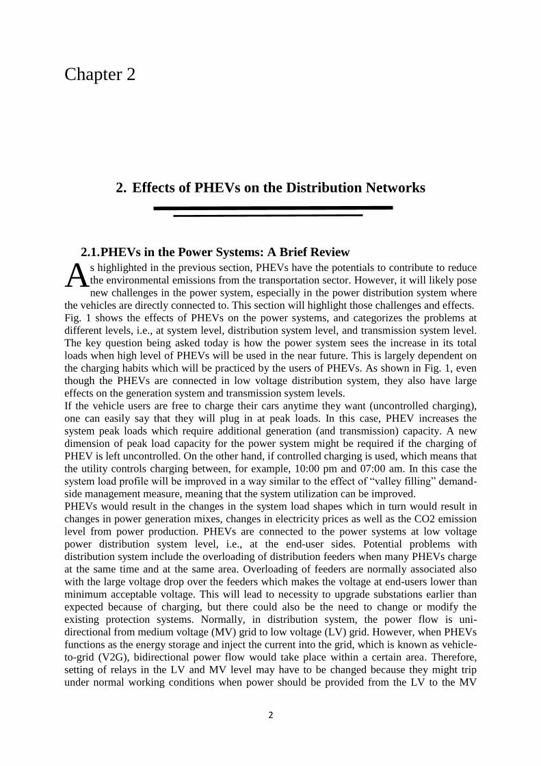
2.1. PHEVs in the Power Systems: A Brief Review

s highlighted in the previous section, PHEVs have the potentials to contribute to reduce

the environmental emissions from the transportation sector. However, it will likely pose

new challenges in the power system, especially in the power distribution system where

the vehicles are directly connected to. This section will highlight those challenges and effects.

Fig. 1 shows the effects of PHEVs on the power systems, and categorizes the problems at

different levels, i.e., at system level, distribution system level, and transmission system level.

The key question being asked today is how the power system sees the increase in its total

loads when high level of PHEVs will be used in the near future. This is largely dependent on

the charging habits which will be practiced by the users of PHEVs. As shown in Fig. 1, even

though the PHEVs are connected in low voltage distribution system, they also have large

effects on the generation system and transmission system levels.

If the vehicle users are free to charge their cars anytime they want (uncontrolled charging),

one can easily say that they will plug in at peak loads. In this case, PHEV increases the

system peak loads which require additional generation (and transmission) capacity. A new

dimension of peak load capacity for the power system might be required if the charging of

PHEV is left uncontrolled. On the other hand, if controlled charging is used, which means that

the utility controls charging between, for example, 10:00 pm and 07:00 am. In this case the

system load profile will be improved in a way similar to the effect of “valley filling” demand-

side management measure, meaning that the system utilization can be improved.

PHEVs would result in the changes in the system load shapes which in turn would result in

changes in power generation mixes, changes in electricity prices as well as the CO2 emission

level from power production. PHEVs are connected to the power systems at low voltage

power distribution system level, i.e., at the end-user sides. Potential problems with

distribution system include the overloading of distribution feeders when many PHEVs charge

at the same time and at the same area. Overloading of feeders are normally associated also

with the large voltage drop over the feeders which makes the voltage at end-users lower than

minimum acceptable voltage. This will lead to necessity to upgrade substations earlier than

expected because of charging, but there could also be the need to change or modify the

existing protection systems. Normally, in distribution system, the power flow is uni-

directional from medium voltage (MV) grid to low voltage (LV) grid. However, when PHEVs

functions as the energy storage and inject the current into the grid, which is known as vehicle-

to-grid (V2G), bidirectional power flow would take place within a certain area. Therefore,

setting of relays in the LV and MV level may have to be changed because they might trip

under normal working conditions when power should be provided from the LV to the MV

A

3

level. Depending on the design of charging system, either it is one-phase charging or three-

phase charging, the load unbalance might occur with the one-phase charging if the

distributions of PHEVs between the phases are unequal. A more comprehensive review of the

effects of PHEVs on the power systems can be found in [7].

Figure 1: Overview of possible effects of PHEVs on power systems

The above mentioned problems, however, are dependent on the characteristics of the grid in

question, number of PHEVs in the areas, types of charging, time of charging, and so on. More

specific research would have to be done in order to answer specific questions related to each

grid. The next section will provide a specific analysis of the effects of PHEVs on the IEEE

Test Distribution System and a real distribution network in the Gothenburg. The effects will

be focused on the overloading of the distribution feeders and the voltage problems at the

customers position.

4

2.2. Effect analysis of PHEVs on the IEEE 13 –Node test distribution systems

For better investigation of the effects of PHEVs on the distribution network, charging of the

vehicles has been simulated on the modified IEEE 13-Node test system with specific load

profile. Both quick and normal charging has been considered at this part.

2.2.1. Description of IEEE 13 –Node test distribution systems

Fig. 2 shows the single line diagram of the IEEE 13-Node Test Feeder [8]. This test system

includes

- 13 buses with voltages of 115KV, 4.16KV and 0.48 KV.

- 9 loads

- 2 transformers.

- 2 capacitors at bus 611 and 675.

Bus number 693 has been added just for connecting transformer to the line. 9 other loads have

been added to the test system for simulating the PHEVs.

Figure 2: IEEE 13-Node test system without PHEVs.

The system is appropriately modified to simulate distribution supply system for a small

residential area. The data has been modified in order to use three-phase power flow analysis

5

software Power World. Table 1 shows the lines resistances and reactances. The Zbase for the

4.16 kV network is 0.173Ω and for 115 kV is 132.25 Ω.

Table 1: Lines impedances

Node A Node B

Total

Resistance in

ohm

Total reactance

in ohm Total R in PU Total X in PU

632 645 0.13 0.13 0.73 0.74

632 633 0.01 0.04 0.09 0.23

633 634 0.00 0.00 0.00 0.00

645 646 0.08 0.08 0.44 0.44

650 632 0.13 0.38 0.76 2.22

684 652 0.20 0.08 1.17 0.45

632 671 0.13 0.38 0.76 2.22

671 684 0.07 0.08 0.43 0.44

671 680 0.07 0.19 0.38 1.11

671 692 0.00 0.00 0.00 0.00

684 611 0.02 0.06 0.11 0.33

692 675 0.08 0.05 0.44 0.28

For having a load profile for all 24 hours of a typical day, the load of the different busses of

the IEEE 13 busses network have been multiplied by a series of 24 numbers each between 0

and 1, corresponding to hours of a typical day. This series of 24 numbers has been obtained

by dividing each hour load by the maximum load of a typical load profile according to [9] .

Figure 3 shows how this load profile looks like for a typical day. The power flow analysis for

this system is done using the Power World Simulator. In this network, the maximum load is

4.82 MW at 6:00 PM and minimum load is 3.02 MW at 3:00 AM. It is assumed that this

network supplies a residential area. According to [10] and [11], each 25 kVA distribution

feeder can approximately serve 4 houses and it can be assumed that every 4 houses will own 2

PHEVs. From this assumption, the number of PHEVs at each bus will be calculated as in (1):

(1).

Where:

NPHEV: Estimated number of PHEVs at each bus

Smax: Maximum supplied kVA at each bus

6

Figure3: Test system Load profile of a typical day.

The PHEV for this investigation is Chevy Volt. Chevy Volt is equipped with a Lithium Ion

Battery [12]. In principle there are two methods of charging: normal charging and quick

charging.

A Chevy Volt usually uses 50-60% of the battery to travel 40 miles in all electric modes.

Assuming that each PHEV commutes a round trip of 40 miles 5 days a week then it will

require a full recharge of around 10 KWh on each day [5]. Based on the calculation in the [11]

the lithium Ion battery of a Chevy volts draws 1.45 KW in 6 to 6.5 hours in normal charging

and also absorbs about 5.8 KW in around 1.7 hour for quick charging after a round trip of 40

miles. The efficiency of 87% is assumed for the whole charging process [10].

The following four different cases have been considered in this study:

- Business as usual (BAU): System at peak load without PHEVs.

- Normal charging, peak load: BAU with PHEVs normal charging.

- Quick charging, peak load: BAU with PHEVs quick charging.

- Quick charging, min load: System at min load with PHEVs quick charging.

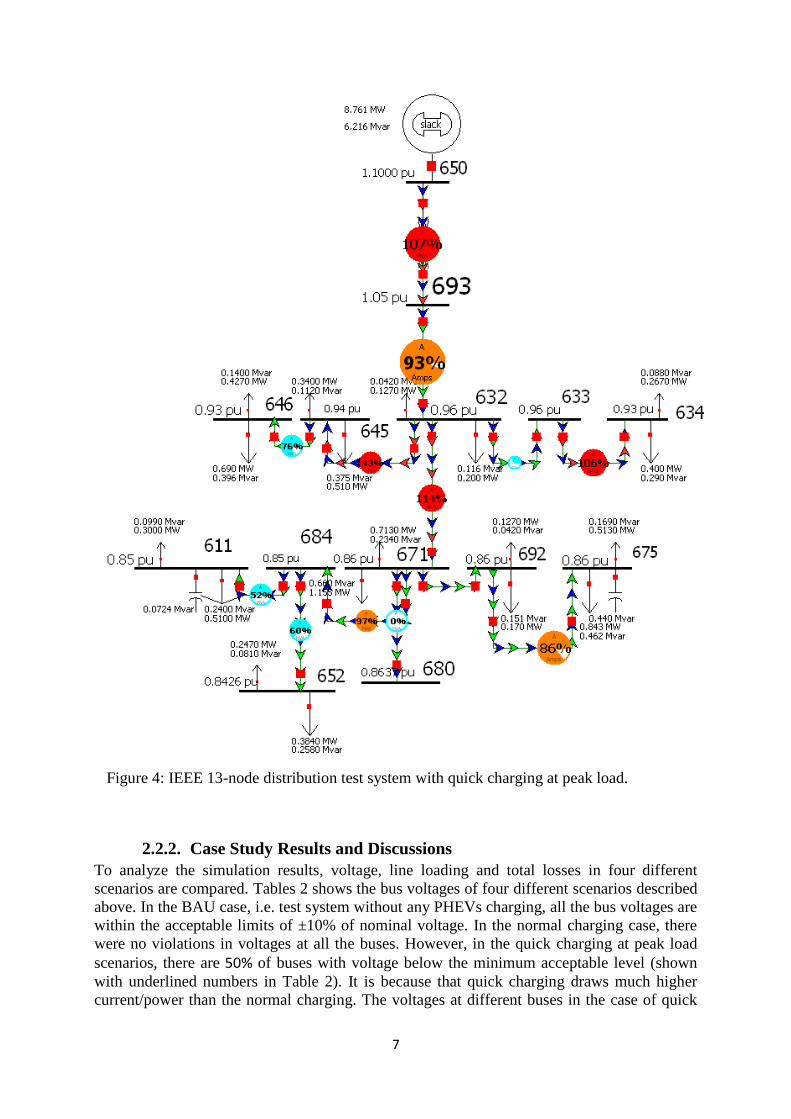
Figure 4 indicates how the simulation file looks like. The upward loads simulate the PHEVs

which are connected to grid.

0

1000

2000

3000

4000

5000

6000

1 3 5 7 9 11 13 15 17 19 21 23

Po

wer

in

Kw

Time of a day in hour

7

2.2.2. Case Study Results and Discussions

To analyze the simulation results, voltage, line loading and total losses in four different

scenarios are compared. Tables 2 shows the bus voltages of four different scenarios described

above. In the BAU case, i.e. test system without any PHEVs charging, all the bus voltages are

within the acceptable limits of ±10% of nominal voltage. In the normal charging case, there

were no violations in voltages at all the buses. However, in the quick charging at peak load

scenarios, there are 50% of buses with voltage below the minimum acceptable level (shown

with underlined numbers in Table 2). It is because that quick charging draws much higher

current/power than the normal charging. The voltages at different buses in the case of quick

Figure 4: IEEE 13-node distribution test system with quick charging at peak load.

8

0,00

0,20

0,40

0,60

0,80

1,00

1,20

61

1

63

2

63

3

63

4

64

5

64

6

65

0

65

2

67

1

67

5

68

0

68

4

69

2

69

3

Vo

ltag

e in

PU

Bus #

BAU scenario

quick charging at

peak load

charging at max load are also shown in Fig. 4 above. If quick charging can be controlled and

done during the min load period, there were no problem of voltage violations in the system as

shown in Table 2.

Table 2: Buses voltages in per unit for different scenarios

BUS # BAU

Normal

Charging, Peak

Load

Quick

Charging,Peak

Load

Quick Charging

Min Load

611 0.97 0.95 0.85 0.96

632 1.03 1.01 0.96 1.02

633 1.03 1.01 0.96 1.02

634 1.00 0.99 0.93 1.00

645 1.01 1.00 0.94 1.00

646 1.01 0.99 0.93 1.00

650 1.10 1.10 1.10 1.10

652 0.96 0.94 0.84 0.95

671 0.97 0.95 0.86 0.97

675 0.97 0.95 0.86 0.96

680 0.97 0.95 0.86 0.97

684 0.97 0.95 0.85 0.96

692 0.97 0.95 0.86 0.97

693 1.07 1.07 1.05 1.07

Figure 5 indicates voltage of different busses in the two scenarios of quick charging at peak

load and BAU which is a comparison between the worst case and BAU.

Figure 5: Bus voltages in BAU and quick charging at peak load

9

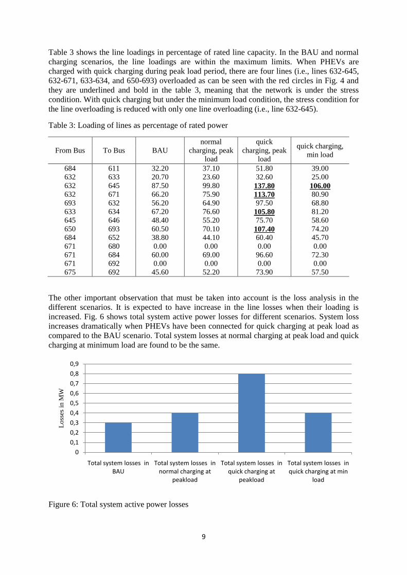
Table 3 shows the line loadings in percentage of rated line capacity. In the BAU and normal

charging scenarios, the line loadings are within the maximum limits. When PHEVs are

charged with quick charging during peak load period, there are four lines (i.e., lines 632-645,

632-671, 633-634, and 650-693) overloaded as can be seen with the red circles in Fig. 4 and

they are underlined and bold in the table 3, meaning that the network is under the stress

condition. With quick charging but under the minimum load condition, the stress condition for

the line overloading is reduced with only one line overloading (i.e., line 632-645).

Table 3: Loading of lines as percentage of rated power

From Bus To Bus BAU

normal

charging, peak

load

quick

charging, peak

load

quick charging,

min load

684 611 32.20 37.10 51.80 39.00

632 633 20.70 23.60 32.60 25.00

632 645 87.50 99.80 137.80 106.00

632 671 66.20 75.90 113.70 80.90

693 632 56.20 64.90 97.50 68.80

633 634 67.20 76.60 105.80 81.20

645 646 48.40 55.20 75.70 58.60

650 693 60.50 70.10 107.40 74.20

684 652 38.80 44.10 60.40 45.70

671 680 0.00 0.00 0.00 0.00

671 684 60.00 69.00 96.60 72.30

671 692 0.00 0.00 0.00 0.00

675 692 45.60 52.20 73.90 57.50

The other important observation that must be taken into account is the loss analysis in the

different scenarios. It is expected to have increase in the line losses when their loading is

increased. Fig. 6 shows total system active power losses for different scenarios. System loss

increases dramatically when PHEVs have been connected for quick charging at peak load as

compared to the BAU scenario. Total system losses at normal charging at peak load and quick

charging at minimum load are found to be the same.

Figure 6: Total system active power losses

0

0,1

0,2

0,3

0,4

0,5

0,6

0,7

0,8

0,9

Total system losses in BAU

Total system losses in normal charging at

peakload

Total system losses in quick charging at

peakload

Total system losses in quick charging at min

load

Lo

sses

in M

W

10

2.3. Effect of PHEVs on the Gothenburg Distribution Network

To analyze the effects of PHEVs charging on a real network, this effect has been tested on a

part of Gothenburg distribution network. This part of Gothenburg distribution network

includes voltage level of 10 and 0.4 kV. There are different areas in this city, some of them

are residential, some others commercial and others are industrial. There are many areas which

are combination of residential, commercial and industrial areas. The load profile of these

areas is totally different. To have a precise investigation, in this master thesis, both 10 kV and

400 V network have been simulated and analyzed for commercial and residential area.

2.3.1. Description of Gothenburg Residential Distribution network (400 V)

In this part, one residential area has been selected to investigate the effect of PHEVs charging

on a real distribution network. The selected area is substation RS1 in the Gothenburg. This

substation includes two transformers of 10 kV/0.4 kV with rating of 500 kVA. This substation

serves for around 144 household customers and is supplied by busbar RBB1 in one 130 to 10

kV Substation. Every hour load profile of line RF1 in year 2008 which is the supplier feeder

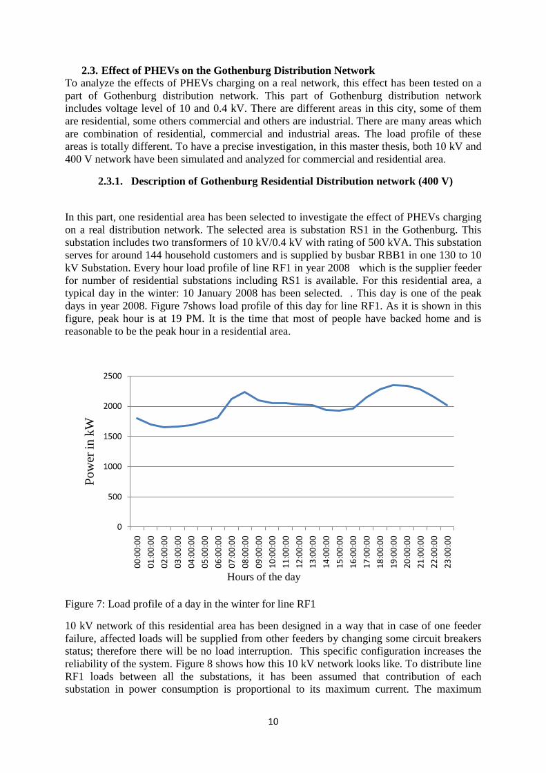
for number of residential substations including RS1 is available. For this residential area, a

typical day in the winter: 10 January 2008 has been selected. . This day is one of the peak

days in year 2008. Figure 7shows load profile of this day for line RF1. As it is shown in this

figure, peak hour is at 19 PM. It is the time that most of people have backed home and is

reasonable to be the peak hour in a residential area.

Figure 7: Load profile of a day in the winter for line RF1

10 kV network of this residential area has been designed in a way that in case of one feeder

failure, affected loads will be supplied from other feeders by changing some circuit breakers

status; therefore there will be no load interruption. This specific configuration increases the

reliability of the system. Figure 8 shows how this 10 kV network looks like. To distribute line

RF1 loads between all the substations, it has been assumed that contribution of each

substation in power consumption is proportional to its maximum current. The maximum

0

500

1000

1500

2000

2500

00

:00

:00

01

:00

:00

02

:00

:00

03

:00

:00

04

:00

:00

05

:00

:00

06

:00

:00

07

:00

:00

08

:00

:00

09

:00

:00

10

:00

:00

11

:00

:00

12

:00

:00

13

:00

:00

14

:00

:00

15

:00

:00

16

:00

:00

17

:00

:00

18

:00

:00

19

:00

:00

20

:00

:00

21

:00

:00

22

:00

:00

23

:00

:00

Po

wer

in

kW

Hours of the day

11

current of all the transformers at each substation are available. In the substations with more

than one transformer, maximum current is summation of all the transformers at that

substation. The load of substations supplied by the line RF1 in normal condition is calculated

as in (2.1).

Pi=PlineRF1×ai (2.1)

Where:

Pi: substation (i) load on 10 January 2008 at 19 PM

PlineRF1: total line RF1 power consumption on 10 January 2008 at 19 PM

ai: distribution coefficient of each substation and is calculated as in (2.2).

ai= and (2.2)

Where:

: Each substation maximum current calculated as in (2.3)

(2.3)

Where

: Maximum current of transformer j at substation i

Substation RS1 load has been distributed between two transformer proportional to their

maximum current. To calculate each bus load in substation RS1, this substation total load:

PRS1 calculated in (2.1), has been distributed between different busses proportionally to their

average annually energy consumption. Annual energy consumption of all the customers was

provided by Göteborg Energy and therefore power of each bus at substation RS1 is calculated

as in (2.4):

Pj=PRS1×bj (2.4)

Where:

Pj: Power of bus j in substation RS1 on day 10 January 2008 at 19PM

bj: distribution coefficient of bus j in substation RS1 and calculated as in (2.5):

bj= and (2.5)

Where:

AAECj: Average Annual Energy Consumption of bus j at substation RS1 and is calculated as

in (2.6):

12

AAECj= (2.6):

Where:

AECj: Annual Energy Consumption of customer j and is provided by the Göteborg Energy.

Figure 8: 10 kV residential network in Gothenburg

For residential area, power factor of each load has been considered to be 0.95 lag and then the

reactive power at each bus will be as in (2.7):

Qj=Pj×TAN (ACOS (0.95)) (2.7)

RS6

RS2

RS3

RS8 RS1

RS7

RS5

RS4

RF2 RF1 RF3

RBB1

13

144 PHEVs has been assumed for the residential area supplied by substation RS1 according to

[13] .These vehicles have been distributed proportionally to buses load. That’s because the

probability of plugging PHEVs in different buses can be proportional to the buses load, in

other word the probability of plugging a vehicle at bus with higher load is more than the

probability of plugging a vehicle to the buss with lower load. Therefore the number of

vehicles at each buss can be calculated as in (2.8):

Nj=144×Proj (2.8):

Where:

Nj: probable number of vehicles at bus j in substation RS1

Proj: probability of having a PHEV at bus j in the substation RS1 connected for charging

which is calculated as in (2.9).

Proj= (2.9)

Where:

Pj: Power of bus j at substation RS1 on day 10 January 2008 at 19 PM

Figure 9 shows the number of vehicles at each bus at substation RS1 only for transformer 2.

Figure 9: Calculated probable number of vehicles at substation RS1 only for transformer 2

It is supposed that vehicles are charged via a plug of 16 A, therefore the power drawn by the

vehicle will be 16A×230V 3.6 kW and also battery and total charging equipment have a

power factor of 0.95. Therefore required power at each bus for charging the vehicles will be

as in (2.10)

PPHEVs(j)= Nj 3.6 kW (2.10)

0

5

10

15

20

25

30

55

58

0

67

47

1

67

52

0

67

51

9

67

47

4

67

52

1

59

28

1

55

05

4

53

56

4

54

74

8

55

60

3

54

90

6

67

47

0

59

21

2

67

11

9

59

28

7

67

47

2

59

21

1

67

11

1

59

37

3

67

47

7

EH1

96

7,0

4. 1

1

EH1

96

7,0

4. 1

2

EH1

96

7,0

4. 1

3

No o

f V

ehic

les

Bus name

14

QPHEVs(j)= PPHEVs(j) TAN(ACOS(0.95))

Where:

PPHEVs(j): required power for charging the vehicles at bus (j)

QPHEVs(j): required reactive power for charging the vehicles at bus (j)

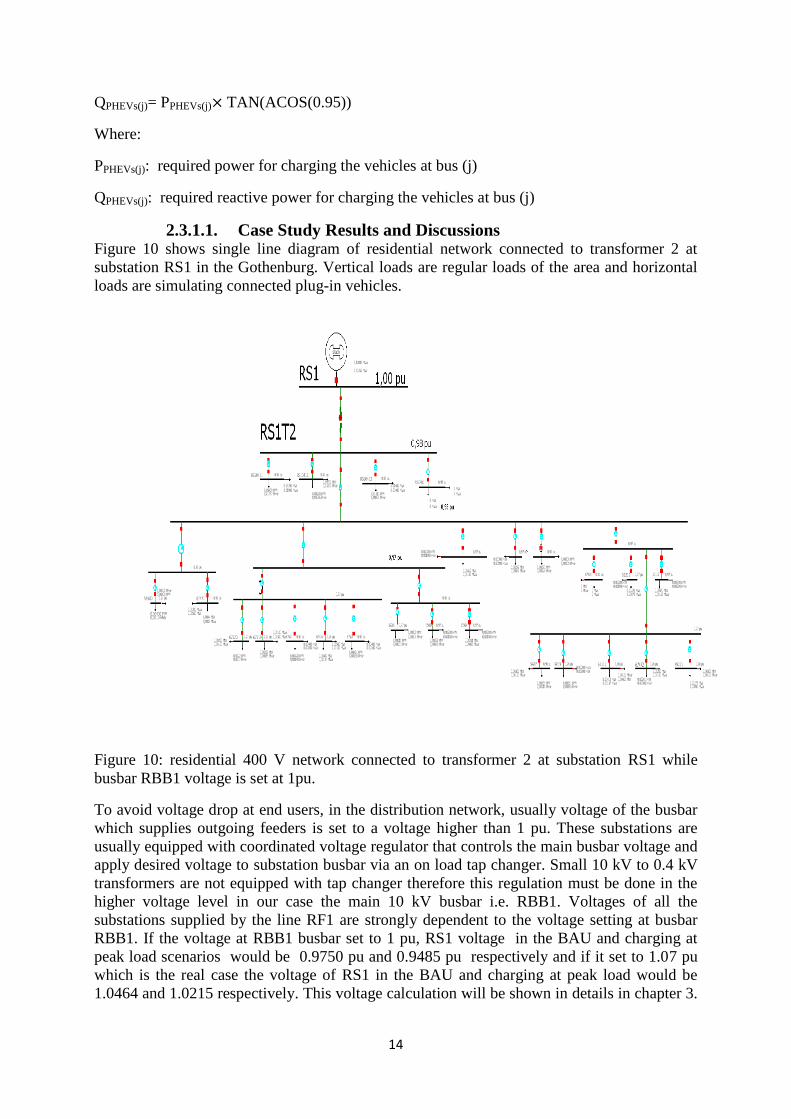
2.3.1.1. Case Study Results and Discussions Figure 10 shows single line diagram of residential network connected to transformer 2 at

substation RS1 in the Gothenburg. Vertical loads are regular loads of the area and horizontal

loads are simulating connected plug-in vehicles.

Figure 10: residential 400 V network connected to transformer 2 at substation RS1 while

busbar RBB1 voltage is set at 1pu.

To avoid voltage drop at end users, in the distribution network, usually voltage of the busbar

which supplies outgoing feeders is set to a voltage higher than 1 pu. These substations are

usually equipped with coordinated voltage regulator that controls the main busbar voltage and

apply desired voltage to substation busbar via an on load tap changer. Small 10 kV to 0.4 kV

transformers are not equipped with tap changer therefore this regulation must be done in the

higher voltage level in our case the main 10 kV busbar i.e. RBB1. Voltages of all the

substations supplied by the line RF1 are strongly dependent to the voltage setting at busbar

RBB1. If the voltage at RBB1 busbar set to 1 pu, RS1 voltage in the BAU and charging at

peak load scenarios would be 0.9750 pu and 0.9485 pu respectively and if it set to 1.07 pu

which is the real case the voltage of RS1 in the BAU and charging at peak load would be

1.0464 and 1.0215 respectively. This voltage calculation will be shown in details in chapter 3.

15

To show advantages of this voltage regulation, investigation of residential network has been

done for two cases:

- RBB1 busbar voltage is set to 1 pu.

- RBB1 busbar voltage is set to 1.07 pu.

For each of above situation two following scenarios have been considered.

- BAU: System at peak load i.e. 19 PM on day 10 January 2008 without any PHEVs

- Simultaneous charging of all PHEVs at peak load

Table 4: Buses voltages in per unit while RBB1 busbar voltage is 1pu.

Bus name BAU Charging at peak load

RS1 0.98 0.95 RS1T2 0.97 0.93 12657 0.96 0.92 13507 0.96 0.92 13677 0.96 0.92 13687 0.96 0.91 15387 0.96 0.92 15397 0.96 0.92 15407 0.96 0.92 13567 0.96 0.92

1547487 0.96 0.92 1549067 0.96 0.92

1054 0.96 0.92 1580 0.96 0.92 1603 0.96 0.92 1111 0.96 0.91 1212 0.96 0.92 8181 0.96 0.92 8787 0.96 0.91 7373 0.96 0.91 6767 0.96 0.91

1671197 0.96 0.91 470470 0.96 0.92 471471 0.96 0.92 472472 0.96 0.91 474474 0.96 0.91 477477 0.96 0.92 519519 0.96 0.92 520520 0.96 0.92 521521 0.96 0.91

RS10411 0.95 0.90 RS10412 0.95 0.89 RS10413 0.96 0.92 RS104bc 0.97 0.93

16

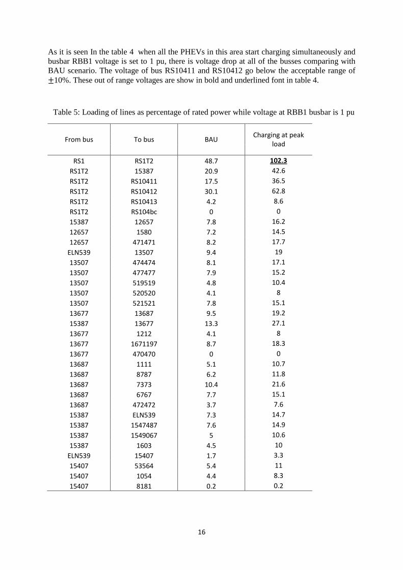
As it is seen In the table 4 when all the PHEVs in this area start charging simultaneously and

busbar RBB1 voltage is set to 1 pu, there is voltage drop at all of the busses comparing with

BAU scenario. The voltage of bus RS10411 and RS10412 go below the acceptable range of

10%. These out of range voltages are show in bold and underlined font in table 4.

Table 5: Loading of lines as percentage of rated power while voltage at RBB1 busbar is 1 pu

From bus To bus BAU Charging at peak

load

RS1 RS1T2 48.7 102.3

RS1T2 15387 20.9 42.6

RS1T2 RS10411 17.5 36.5

RS1T2 RS10412 30.1 62.8

RS1T2 RS10413 4.2 8.6

RS1T2 RS104bc 0 0

15387 12657 7.8 16.2

12657 1580 7.2 14.5

12657 471471 8.2 17.7

ELN539 13507 9.4 19

13507 474474 8.1 17.1

13507 477477 7.9 15.2

13507 519519 4.8 10.4

13507 520520 4.1 8

13507 521521 7.8 15.1

13677 13687 9.5 19.2

15387 13677 13.3 27.1

13677 1212 4.1 8

13677 1671197 8.7 18.3

13677 470470 0 0

13687 1111 5.1 10.7

13687 8787 6.2 11.8

13687 7373 10.4 21.6

13687 6767 7.7 15.1

13687 472472 3.7 7.6

15387 ELN539 7.3 14.7

15387 1547487 7.6 14.9

15387 1549067 5 10.6

15387 1603 4.5 10

ELN539 15407 1.7 3.3

15407 53564 5.4 11

15407 1054 4.4 8.3

15407 8181 0.2 0.2

17

Table 5 shows different lines percentage loading while busbar RBB1 voltage is set to 1 pu.

This table indicates that all the lines loading increase in charging at peak load scenario

comparing to BAU. In the BAU scenario there is no overloaded line, however, line from bus

RS1 to RS1T2 is overloaded in charging at peak load scenario.

Table 6: Buses voltages in per unit for different scenarios while RBB1 voltage is 1.07pu

Bus name BAU Charging at peak load

RS1 1.05 1.02 RS1T2 1.04 1.00 12657 1.04 1.00 13507 1.03 0.99 13677 1.03 0.99 13687 1.03 0.99 15387 1.04 1.00

ELN539 1.03 1.00 15407 1.03 1.00 53564 1.03 0.99

1547487 1.03 0.99 1549067 1.03 1.00

1054 1.03 0.99 1580 1.03 0.99 1603 1.04 1.00 1111 1.03 0.99 1212 1.03 0.99 8181 1.03 1.00 8787 1.03 0.99 7373 1.03 0.98 6767 1.03 0.98

1671197 1.03 0.99 470470 1.03 0.99 471471 1.03 0.99 472472 1.03 0.99 474474 1.03 0.99 477477 1.03 0.99 519519 1.03 0.99 520520 1.03 0.99 521521 1.03 0.99

RS10411 1.03 0.98 RS10412 1.02 0.96 RS10413 1.03 0.99 RS104bc 1.04 1.00

Table 6 and 7 shows different busses voltage and line loading in the BAU and charging at

peak load scenario while the RBB1 busbar voltage is set to 1.07 pu.

18

Table 7: Loading of lines as percentage of rated power while RBB1 busbar voltage is 1.07 pu

From bus To bus BAU Charging at peak

load

RS1 RS1T2 48.7 102

RS1T2 15387 20.8 42.2

RS1T2 RS10411 17.4 36

RS1T2 RS10412 29.8 62.1

RS1T2 RS10413 4.2 8.6

RS1T2 RS104bc 0 0

15387 12657 7.7 16.1

12657 1580 7.2 14.4

12657 471471 8.2 17.6

ELN539 13507 9.4 18.8

13507 474474 8 17

13507 477477 7.9 15.1

13507 519519 4.8 10.3

13507 520520 4.1 8

13507 521521 7.8 15

13677 13687 9.4 19

15387 13677 13.2 26.8

13677 1212 4.1 8

13677 1671197 8.7 18.1

13677 470470 0 0

13687 1111 5.1 10.6

13687 8787 6.2 11.7

13687 7373 10.3 21.4

13687 6767 7.7 14.9

13687 472472 3.7 7.6

15387 ELN539 7.3 14.6

15387 1547487 7.6 14.8

15387 1549067 5 10.6

15387 1603 4.4 10

ELN539 15407 1.7 3.3

15407 53564 5.4 10.9

15407 1054 4.4 8.2

15407 8181 0.2 0.2

As it is seen in the tables 6, after setting the busbar RBB1 voltage to 1.07 pu, there is no

under voltage at any buses nor in BAU neither in charging at peak load scenario. Line

loading percentage for all the lines in this situation is shown in the table 7. There is no

overloading line in the BAU scenario however line from RS1 to RS1T2 is overloaded in the

charging at peak load scenario.

19

2.3.2. Description of Gothenburg Commercial Distribution network (400 V)

In this part, one commercial area has been selected to investigate the effect of PHEVs

charging on a real distribution network. Selected area is substation CS1 in the Gothenburg.

This substation includes two transformers of 10 kV/ 0.4 kV with rating of 750 and 1250 kVA.

This substation serves for around 115 commercial customers and is one substation of 10 kV

network supplied by busbar CBB1 and CBB2 in one 130 to 10 kV Substation. This 10 kV

network has been made up of 4 lines named CF1, CF2, CF3, and CF4. Every hour load profile

of all these four lines in year 2008 is available. For this commercial area, a typical day in the

winter: 14 February 2008 has been selected. This day is one of the peak days in this year.

Figure 11shows this 10 kV network load profile i.e. summation of line CF1, CF2, CF3, and

CF4 power on 14 February 2008. As it is shown in this figure, peak hour is at 12 PM.

Figure 11: load profile of the 10 kV network supplying a commercial area in the Gothenburg

on 14 February 2008.

This commercial area 10 kV network is designed in a way that in case of one feeder failure ,

affected load, is fed from other feeders by changing some circuit breakers status. Figure 12

shows how this 10 kV network looks like. To distribute this commercial 10 kV network load

between all substations, it has been assumed that contribution of each substation in load

consumption is proportional to its maximum transformer current. The maximum current of all

the transformers are available. In substations with more than one transformer, maximum

current is summation of all the transformers at that substation. Each substation load is

calculated according to (2.11):

Pi=P10kV network×ai (2.11)

Where:

Pi: load of substation (i) at peak load on day 14 February 2008.

P10kVring: Total power of 10 kV commercial network i.e. summation of lines CF1, CF2, CF3,

and CF4 loads at peak load on day 14 February 2008.

ai: each substation distribution coefficient and is calculated as in (2.12):

0

1000

2000

3000

4000

5000

6000

7000

00

:00

:00

01

:00

:00

02

:00

:00

03

:00

:00

04

:00

:00

05

:00

:00

06

:00

:00

07

:00

:00

08

:00

:00

09

:00

:00

10

:00

:00

11

:00

:00

12

:00

:00

13

:00

:00

14

:00

:00

15

:00

:00

16

:00

:00

17

:00

:00

18

:00

:00

19

:00

:00

20

:00

:00

21

:00

:00

22

:00

:00

23

:00

:00

Po

wer

in

kW

Hours of the day

20

ai= and = 1 (2.12)

Where:

: Maximum current of each substation calculated as in (2.13)

(2.13)

Where

: Maximum current of transformer j in substation i

Load at substation CS1 has been distributed between two transformers proportionally to their

maximum current. For calculation each bus load in substation CS1, total load of this

substation: PCS1 calculated by (2.11), has been distributed between different busses

proportionally to their average annually energy consumption. The annual energy consumption

of all the customers was provided by Göteborg Energy and therefore power of each bus at

substation CS1 is calculated as in (2.14):

Pj=PCS1×bj (2.14)

Where:

Pj: bus j Power in substation CS1 at peak load on day 14 February 2008.

bj: bus j distribution coefficient in substation CS1 and calculated as in (2.15):

bj= and (2.15)

Where:

AAECj is Average Annual Energy Consumption of bus j in substation CS1 and is calculated

as in (2.16)

AAECj= (2.16)

Where:

AECj: Annual Energy Consumption of customer j and is provided by the Göteborg Energy.

21

Figure 12: 10 kV network of a commercial area in the Gothenburg

For this commercial area, power factor of each load has been considered to be 0.95 lag and

then the reactive power at each bus will be as in (2.17):

Qj=Pj×TAN (ACOS (0.95)) (7)

It is assumed there are 148 vehicles at commercial area at peak load and demand for charging.

This number of PHEVs has been obtained according to the day time number of vehicles at

this commercial area [13]. The probability of plugging PHEVs in different busses can be

proportional to buses load, in other word probability of plugging a vehicle at bus with higher

load is more than the probability of plugging a vehicle to the buss with lower load. Therefore

the probable number of vehicles at each buss can be calculated as in (2.18):

CF1

CS3

CS4

CS5

CS6

CS7

CS8

CS9

CS10

CS1

CS2

CF3

CF2

CF4

CS11

CBB2

CBB1

22

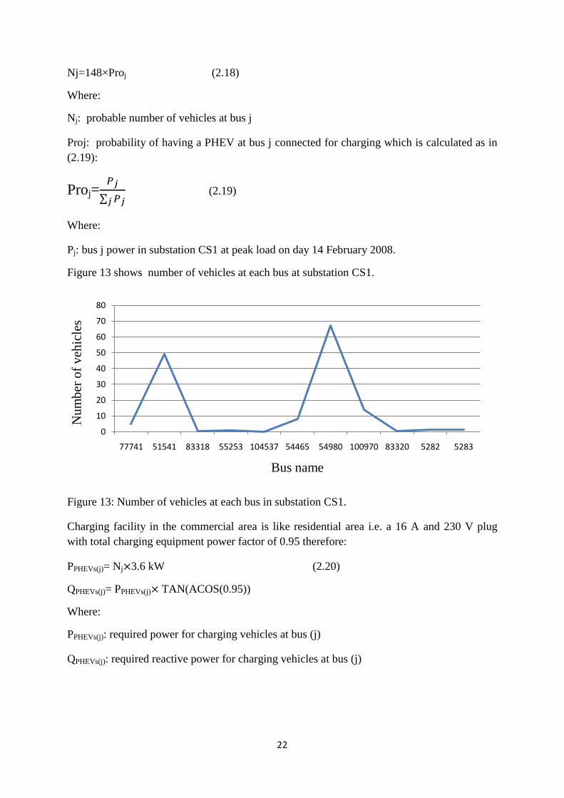
Nj=148×Proj (2.18)

Where:

Nj: probable number of vehicles at bus j

Proj: probability of having a PHEV at bus j connected for charging which is calculated as in

(2.19):

Proj= (2.19)

Where:

Pj: bus j power in substation CS1 at peak load on day 14 February 2008.

Figure 13 shows number of vehicles at each bus at substation CS1.

Figure 13: Number of vehicles at each bus in substation CS1.

Charging facility in the commercial area is like residential area i.e. a 16 A and 230 V plug

with total charging equipment power factor of 0.95 therefore:

PPHEVs(j)= Nj 3.6 kW (2.20)

QPHEVs(j)= PPHEVs(j) TAN(ACOS(0.95))

Where:

PPHEVs(j): required power for charging vehicles at bus (j)

QPHEVs(j): required reactive power for charging vehicles at bus (j)

0

10

20

30

40

50

60

70

80

77741 51541 83318 55253 104537 54465 54980 100970 83320 5282 5283

Nu

mb

er o

f veh

icle

s

Bus name

23

2.3.2.1. Case Study Results and Discussions

In this part, simulation results for mentioned commercial area are presented and analyzed in

details. Figure 14 and 15 show single line diagram of two transformers and their outgoing

feeders at substation CS1 in the Gothenburg. Vertical loads are the regular loads of the

commercial area and horizontal loads are simulating plugged in vehicles.

Figure 14: Single line diagram of commercial 400 V network connected to transformer 1at

substation CS1.

Substation CS1 voltage with and without PHEVs in the 10 kV network is 1.0641 and 1.0643

respectively. Calculation of these voltages has been explained in chapter 3 in details.

24

Figure 15: Single line diagram of commercial 400 V network connected to transformer 2 at

substation CS1.

Table 7 and 8, shows bus voltages and line loading for two different cases:

- BAU: System at peak load i.e. on day 14 February 2008 at 12 PM without any PHEVs

- Simultaneous charging of all PHEVs at peak load

As it is observed in the table 7, there is no considerable voltage drop when PHEVs start to

charge simultaneously. That’s mainly because of large cross section of cables in this area. The

voltage difference in the BAU and charging at peak load is quite negligible.

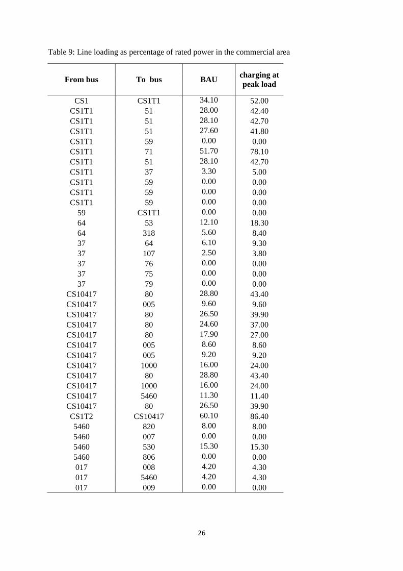
Table 8 shows loading of the lines in two different cases. Line loading increases in charging at

peak load scenario but there is no over loaded line yet.

25

Table 8: Buses voltages in per unit for different scenarios in commercial area

Bus # BAU Charging at

peak load

CS1 1.06 1.06

318 1.05 1.05

53 1.05 1.04

CS1T1 1.06 1.05

64 1.05 1.05

37 1.06 1.05

51 1.05 1.04

59 1.06 1.05

71 1.06 1.05

79 1.06 1.05

75 1.06 1.05

76 1.06 1.05

107 1.06 1.05

CS10417 1.05 1.05

820 1.05 1.05

017 1.05 1.05

806 1.05 1.05

530 1.05 1.05

007 1.05 1.05

008 1.05 1.05

009 1.05 1.05

005 1.05 1.05

80 1.05 1.05

1000 1.05 1.04

5460 1.05 1.05

CS1T2 1.06 1.06

26

Table 9: Line loading as percentage of rated power in the commercial area

From bus To bus BAU charging at

peak load

CS1 CS1T1 34.10 52.00

CS1T1 51 28.00 42.40

CS1T1 51 28.10 42.70

CS1T1 51 27.60 41.80

CS1T1 59 0.00 0.00

CS1T1 71 51.70 78.10

CS1T1 51 28.10 42.70

CS1T1 37 3.30 5.00

CS1T1 59 0.00 0.00

CS1T1 59 0.00 0.00

CS1T1 59 0.00 0.00

59 CS1T1 0.00 0.00

64 53 12.10 18.30

64 318 5.60 8.40

37 64 6.10 9.30

37 107 2.50 3.80

37 76 0.00 0.00

37 75 0.00 0.00

37 79 0.00 0.00

CS10417 80 28.80 43.40

CS10417 005 9.60 9.60

CS10417 80 26.50 39.90

CS10417 80 24.60 37.00

CS10417 80 17.90 27.00

CS10417 005 8.60 8.60

CS10417 005 9.20 9.20

CS10417 1000 16.00 24.00

CS10417 80 28.80 43.40

CS10417 1000 16.00 24.00

CS10417 5460 11.30 11.40

CS10417 80 26.50 39.90

CS1T2 CS10417 60.10 86.40

5460 820 8.00 8.00

5460 007 0.00 0.00

5460 530 15.30 15.30

5460 806 0.00 0.00

017 008 4.20 4.30

017 5460 4.20 4.30

017 009 0.00 0.00

27

2.4. Comments on the Protection

PHEVS in the Gothenburg are supposed to be charged via a 220 V 16 ampere single phase

plug. Many of the customers both in the residential and commercial area are using fuse of 20

Ampere for their main feeders. It means in a case that customers are charging their vehicles

cannot use more than 4 amperes corresponding to 4*220=0.88 kW. It can be risky for the

customer especially when it is taken to account that one simple hair dryer has power of

around 1 kW. Maybe the fuses replacement will be inevitable for using the PHEVs. The other

solution can be using three phases plug, then current of each phase will decrease to one third

and it will be safe in terms of the fusing. The protection scheme of the distribution networks is

usually designed for a unidirectional power flow and in a case that vehicles inject power to

the grid; this protection system might be required to be verified.

28

Chapter 3

3. Effects of PHEVs on the Gothenburg 10 kV Network

ffect of PHEVs charging have been investigated on two 400 V distribution network with

residential and commercial characteristic so far. The more important case is accumulated

effect of some similar distribution network when reaches to higher voltage level network

for example 10 kV. In this part of Master thesis, effect of charging PHEVs on a network made

up of number of 10 to 0.4 kV substations will be investigated both for residential and

commercial area. To have an estimation of maximum number of vehicle that can be connected

to grid for charging simultaneously, one iterative method has been used with considering

reliability issues.

3.1. Description of Sample 10 kV Commercial Network in Gothenburg

This sample network is a 10 kV network located in the Gothenburg city. It has been made up

of four 10 kV feeders i.e. CF1, CF2, CF3, CF4 supplied from CBB1 and CBB2 10 kV busbar.

Figure 12 shows how this 10 kV commercial network looks like. It is called a commercial

distribution network, because most of the customers in this area are business offices. The

power consumption of all the outgoing feeders separately and also the aggregation of these

four feeders load consumption is available through the data from Göteborg Energy. For this

study worst case i.e. maximum load of the 10 kV network in normal operation i.e. no feeders

outage in the year 2008 which is 7.632 MW has been considered .To have a fair load

distribution, total loads have been distributed between substations proportionally to the

maximum current drawn by each substation in year 2008. Maximum current of each

transformer are available via the data obtained from Göteborg Energy. According to equation

(2.11) in chapter 2:

Pi=P10kV network×ai

Where:

Pi: load of substation (i) at peak load.

P10kVring: total power of 10 kV commercial network i.e. the summation of lines CF1, CF2,

CF3, and CF4 loads at peak load in the year 2008 which is 7.632 MW.

ai: distribution coefficient of each substation and is calculated as below

ai= and = 1

Where:

E

29

: Maximum current of each substation and calculated as below

Where

: Maximum current of transformer j at substation i

Having calculated each substation load, then probable power required for charging vehicles at

each substation must be calculated. It is assumed that probable number of vehicles at each

substation is proportional to that substation load.

NCS1=Ntotal×ProCS1 (2.21)

Where:

ProCS1: probability of having a vehicles charging at substation CS1 which is calculated as in

(2.22):

Proi= (2.22)

Where:

Pi: load of each substation in 10 kV network

Proi: probability of having a vehicle charging at substation i in the 10 kV network.

So the probable total number of PHEVs at 10 kV network will be

Ntotal= (2.23)

And probable number of vehicle at each substation will be:

Ni=Ntotal× Proi (2.24)

Required power for charging the PHEVs at each substation will be:

PPHEVi= Ni×3.6 kW=

And finally

PPHEVi = =0.51284 (2.25)

Where:

PPHEVi: probable active power required for charging the vehicles at substation i

30

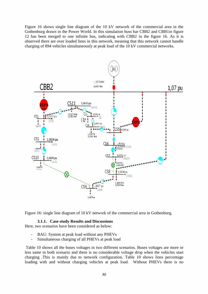
Figure 16 shows single line diagram of the 10 kV network of the commercial area in the

Gothenburg drawn in the Power World. In this simulation buss bar CBB2 and CBB1in figure

12 has been merged to one infinite bus, indicating with CBB2 in the figure 16. As it is

observed there are over loaded lines in this network, meaning that this network cannot handle

charging of 894 vehicles simultaneously at peak load of the 10 kV commercial networks.

Figure 16: single line diagram of 10 kV network of the commercial area in Gothenburg.

3.1.1. Case study Results and Discussions

Here, two scenarios have been considered as below:

- BAU: System at peak load without any PHEVs

- Simultaneous charging of all PHEVs at peak load

Table 10 shows all the buses voltages in two different scenarios. Buses voltages are more or

less same in both scenario and there is no considerable voltage drop when the vehicles start

charging .This is mainly due to network configuration. Table 10 shows lines percentage

loading with and without charging vehicles at peak load. Without PHEVs there is no

31

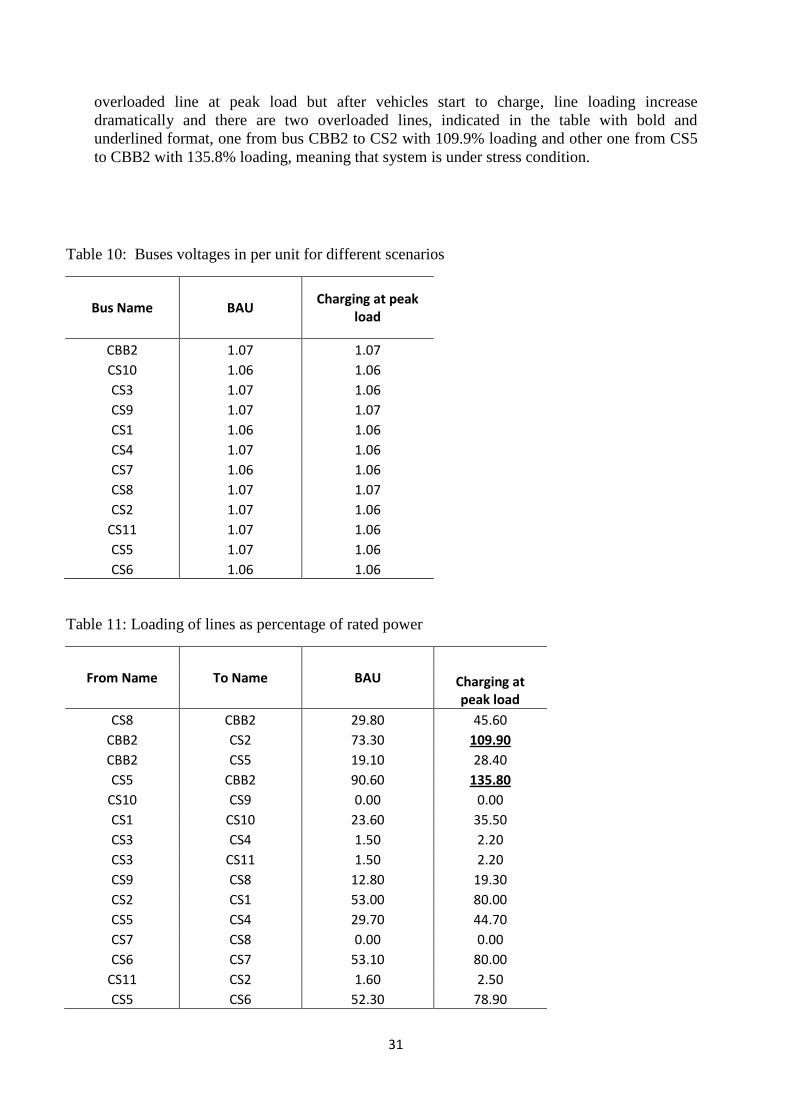
overloaded line at peak load but after vehicles start to charge, line loading increase

dramatically and there are two overloaded lines, indicated in the table with bold and

underlined format, one from bus CBB2 to CS2 with 109.9% loading and other one from CS5

to CBB2 with 135.8% loading, meaning that system is under stress condition.

Table 10: Buses voltages in per unit for different scenarios

Bus Name BAU Charging at peak

load

CBB2 1.07 1.07

CS10 1.06 1.06

CS3 1.07 1.06

CS9 1.07 1.07

CS1 1.06 1.06

CS4 1.07 1.06

CS7 1.06 1.06

CS8 1.07 1.07

CS2 1.07 1.06

CS11 1.07 1.06

CS5 1.07 1.06

CS6 1.06 1.06

Table 11: Loading of lines as percentage of rated power

From Name To Name BAU Charging at peak load

CS8 CBB2 29.80 45.60

CBB2 CS2 73.30 109.90

CBB2 CS5 19.10 28.40

CS5 CBB2 90.60 135.80

CS10 CS9 0.00 0.00

CS1 CS10 23.60 35.50

CS3 CS4 1.50 2.20

CS3 CS11 1.50 2.20

CS9 CS8 12.80 19.30

CS2 CS1 53.00 80.00

CS5 CS4 29.70 44.70

CS7 CS8 0.00 0.00

CS6 CS7 53.10 80.00

CS11 CS2 1.60 2.50

CS5 CS6 52.30 78.90

32

3.2. Description of Sample 10 kV Residential Network in Gothenburg

This sample network is a 10 kV residential network located in the Gothenburg city. It has been

made up of three 10 kV feeders i.e. RF1, RF2, and RF3 supplied from RBB1 10 kV busbar. Figure

8 shows how this 10 kV residential network is. It is called a residential distribution network,

because most of the customers in this area are residential houses. The power consumption of all

the outgoing feeders separately and also the aggregation of these three feeders load consumption is

available through the data from Göteborg Energy. In normal situation, circuit breaker at substation

RS2 is open, so line RF1 supplies all the substation starting from RS3 and ending at RS2 therefore

investigation of residential 10 kV network is limited to one radial configuration starting from RS3

and ending at RS2 as it is shown in the figure 18. Maximum loading of this 10 kV network i.e.

maximum summation of these three feeders in the year 2008 is 7.874 MW and contribution of line

RF1 is 2.815 MW at this peak load.

Similar to commercial area, to have a fair load distribution, total loads have been distributed

proportionally to the maximum current drawn by each substation in year 2008.

Pi=PLineRF1×ai (2.26)

Where:

Pi: load of substation (i) at peak load.

PLineRF1: total power of line RF1 at peak loads i.e. 2.815 MW.

ai: distribution coefficient of each substation supplied by the line RF1 and is calculated as below:

ai= and = 1

Where:

: Maximum current of each substation and calculated as below

Where

: Maximum current of transformer j at substation i

Like the commercial area, having calculated each substation load, then probable power required

for charging vehicles at each substation must be calculated. Here it is assumed that probable

number of vehicles at each substation is proportional to that substation load.

NRS1=Ntotal×ProRS1 (2.27)

Where:

ProRS1: probability of having a vehicles charging at substation RS1 which is calculated as in

(2.27):

Proi= (2.27)

33

Where:

Pi: load of each substation supplied by line RF1

Proi: probability of having a vehicle charging at substation i supplied by line RF1.

So the probable total number of PHEVs at this residential area at peak load will be:

Ntotal= (2.28)

Probable number of vehicle at each substation will be:

Ni=Ntota× Proi

Probable required power for charging the PHEVs at each substation will be:

PPHEVi= Ni×3.6 kW=

And finally

PPHEVi = 1

Where:

PPHEVi: the probable active power required for charging the vehicles at substation i

Figure 17 shows single line diagram of the 10 kV residential network in the Gothenburg drawn in

the Power World. As it is observed, there are over loaded lines in this network, meaning that this

network cannot handle charging of 680 vehicles simultaneously at peak load of the 10 kV

residential network.

34

Figure 17: single line diagram of the 10 kV residential network in the Gothenburg

3.2.1. Case study Results and Discussions

To see effect of charging PHEVs on a real 10 kV residential network, two scenarios like

commercial area have been considered as below:

- BAU: System at peak load without any PHEVs

- Simultaneous charging of all PHEVs at peak load

Table 12 and 13 indicates the result of this case study. As it is seen in the table 12 when

vehicles start charging simultaneously, there is a voltage drop at buses but all the buses

voltages are in the acceptable range in both scenarios. Table 13 indicates line loading as

percentage of their nominal rating. In the BAU scenario there is no overloaded line but in the

charging at peak load scenario there are three overloaded lines i.e. line form bus RBB1 to RS3,

35

line from bus RS3 to RS4 and line from bus RS4 to RS5, indicating that network is under

stress condition.

Table 12: Buses voltages in per unit for different scenarios

Bus # BAU Charging at

peak load

RBB1 1.07 1.07

RS3 1.05 1.03

RS4 1.05 1.03

RS5 1.05 1.02

RS6 1.05 1.03

RS7 1.05 1.02

RS1 1.05 1.02

RS2 1.05 1.02

RS8 1.05 1.02

RS9 1.04 1.02

Table 13: line loading as percentage of rated power

From bus To bus BAU Charging at

peak load

RBB1 RS3 64.10 131.80

RS3 RS4 66.10 133.00

RS3 RS6 7.60 15.20

RS4 RS5 53.00 106.40

RS5 RS7 4.10 8.20

RS5 RS1 36.50 73.10

RS1 RS2 19.20 38.50

RS1 RS8 0.00 0.00

RS2 RS9 0.00 0.00

36

3.3. Calculation maximum number of vehicles that can be charged without any

violation

For the distribution companies (Discos) it is very important to know the maximum number of the

vehicles that can be charged at any time in the distribution network. This number is strongly

dependent to the way that vehicles have been distributed in the distribution network i.e. with

different distribution of charging vehicles; different maximum possible vehicle charging is

obtained. In this part of the master thesis maximum possible charging is obtained for both

commercial and residential 10 kV network in one area in Gothenburg while the most possible

distribution has been considered. Most possible distribution here, is proportional to load, in other

word, it is assumed that the places with more load are more probable to be used for charging the

vehicles. This seems to be a quite fair assumption because in the residential and commercial area,

places with higher load level include more people and consequently more vehicle owners and

finally more vehicles demanding for recharge. In the part 3.1 and 3.2 it was seen that commercial

and residential 10 kV network in the Gothenburg were not able to charge 894 and 680 vehicle

respectively at their peak load because there were some overloaded lines.

Figure 18: flow chart for calculation maximum possible charging

Start with charging at peak load

with calculated total probable

No of vehicles

Decrease the No of charging

vehicles while retaining the

distribution configuration of

vehicles at different busses

Violation

Maximum No of vehicle that can

be charged at peak load with most

probable distribution

Yes

No

37

Figure 18 shows the procedure that has been used for calculation maximum possible vehicle

charging. Based on the procedure illustrated in the figure 18, table14 and figure 19 shows the

maximum possible vehicle charging for the commercial area at its peak load.

Figure 19: Percentage loading of 2 most loaded line in the commercial area versus different

number of charging vehicles

As it is seen in figure 19, two most loaded lines at commercial 10 kV network are line from CS5

to CBB2 and line from CBB2 to CS2. Number of vehicles has been decreases till reaching loading

of 100% for line from CS5 to CBB2. In this network, there is no under voltage, even when all the

vehicles have been connected for charging simultaneously. Therefore considered violation is

overloading of the lines. Figure 19 indicates that number of vehicles charging has been decreased

till 205.62 vehicles that correspond to no overloaded lines. Table 14 shows exact number of the

quantities in figure 19 in the table format.

Table 14: Percentage loading of 2 most loaded line in the commercial area with different number

of charging vesicles’.

Percentage of vehicles

Number of Vehicles Line CS5 to CBB2

percentage loading Line CBB2 to CS2

percentage loading

100 894.00 135 103.00

90 804.60 131 99.00

80 715.20 125 95.00

70 625.80 121 92.00

60 536.40 117 89.00

50 447.00 112 85.00

40 357.60 108 82.00

30 268.20 103 78.00

25 223.50 102 77.30

23 205.62 100 75.70

0

20

40

60

80

100

120

140

160

Per

centa

ge

of

line

load

ing

Number of Vehicles

Line CS5 to CBB2 percentage loading

Line CBB2 to CS2 percentage loading

38

Same procedure has been done for the residential area i.e. number of vehicles has been decreased

till there is no violations in the network. In the residential area like the commercial one the

violation means line over loading and under voltage is not the case in this network.

Figure 20: Percentage loading of 3 most loaded line in the residential area versus different number

of charging vehicles

Figure 20 shows percentage of three most loaded lines in the residential network. As it is seen

number of vehicles has decreased to 380 till there is no line with loading percentage of more than

100%. Table 15 shows the same data in more details.

Table 15: Percentage loading of 3 most loaded line in the residential area with different number of

charging vehicles.

Percentage of

vehicles

Number of

Vehicles

Line RBB1 to

RS3 percentage

loading

Line RS3 to RS4

percentage loading

Line RS4 to RS5

percentage loading

100 680 123 129 104.00

90 612 116 121 98.00

80 544 110 115 92.00

70 476 103 108 87.00

60 408 97 102 82.00

56 380,80 95 100 79.90

0

20

40

60

80

100

120

140

680 612 544 476 408 380,80

Per

cen

tage

of

lin

e lo

adin

g

Number of vehicles

Line: RBB1 to RS3

Line: RS3 to RS4

Line RS4 to RS5

39

3.4. Reliability Issues

Finding maximum number of vehicles that can be charged in the distribution network without any

over loading does not necessarily mean this number of vehicles can be charged in the network

without any problem. In other word system must be capable to meet the loads requirement without

any violation both in the normal condition and fault condition. For example during the time that

vehicles are charging, if a fault happens, there must be at least one path for loads supply without

any over loading. This safe path can be obtained by changing different circuit breakers status in

the network. Figure 21 shows flow chart for the procedure that can be used for the maximum

number of vehicles that can be charged simultaneously without any over loading and in a reliable

manner in terms of feeder failure.

Figure 21: flow chart for checking the system reliability

Having found maximum

number of vehicles that can

be charged simultaneously

without any overloading

Is there at least one possible

network configuration obtained

with and without changing the

CBs status for supplying all the

loads without any over loading

for any line failure.

Decrease the number of vehicles

System is reliable

and this number of

vehicles is

acceptable

Yes

No

40

3.5. Effect of power electronic devices

In the close future, V2G i.e. voltage to grid will be applicable and vehicle batteries will inject

power to grid. The charger of these vehicles are bidirectional, in other word they can flow the

power both from grid to vehicles and also from vehicles to grid. These chargers are equipped with

controllers that are able to set any power factor for the charger. For example they will be capable

to inject pure active or reactive power to grid. This feature will be very useful for mitigation the

violation in the distribution network. For example in a case that there is a voltage drop because of

charging vehicles, some of the vehicles can inject reactive power to the grid for reactive power

compensation and finally mitigate the voltage drop. These chargers are also capable of power

factor correction. In fact they can compensate the other loads inductive current by injection of a

capacitive current.

41

Chapter 4

4. Analysis of PHEVs on the Meshed Transmission Networks

4.1. PHEVs in the Transmission Networks: A Brief Review

s it was shown in Fig. 1, even though the PHEVs are connected in low voltage distribution

system, they also have large effects on the generation system and transmission system

levels. If the vehicle users are free to charge their cars anytime they want (uncontrolled

charging), one can easily say that they will plug in at peak loads. In this case, PHEV increases the

system peak loads which require additional generation (and transmission) capacity. A new

dimension of peak load capacity for the power system might be required if the charging of PHEV

is left uncontrolled. On the other hand, if controlled charging is used, which means that the utility

controls charging between, for example, 10:00 pm and 07:00 am. In this case the system load

profile will be improved in a way similar to the effect of “valley filling” demand-side management

measure, meaning that the system utilization can be improved. So the required power for charging

the vehicles could affect the generation and transmission capacity by demanding more power than

the case without PHEVs. In other hand the interesting feature of the PHEVs from power system

point of view is their capability to inject power to grid when they are parked (V2G). V2G presents

a mechanism to meet power requirement of the power system, using electric vehicles, when they

are parked. The most economic effect of this green feature is the market for ancillary services. The

second interesting feature of V2G is spinning reserve. In the areas with deregulated market this

advantages of V2G is easier to observe. PHEVs are well suited for ancillary services and spinning

reserves because the batteries of the vehicles are quick enough to respond the power demand

required by the power systems [3]. To have a good understanding of PHEVs effects on the

transmission network, two test transmission networks with specified penetration of PHEVs have

been considered in this chapter.

A

42

4.2. Effect Analysis of PHEVs on the 10-Bus Test System

First, effects of PHEVs have been considered on a sample meshed transmission network. The

system description and analysis of this simulation is as below.

4.2.1. Description of 10-Bus system 10 bus systems is a sample transmission network. This system includes:

- 10 busses of 138 kV.

- 7 loads

- 6 generators

- 7 capacitors

7 other loads have added to the PQ busses of this test system for simulation of the PHEVs. Figure

22 shows how this system looks like. The horizontal loads connected to the busses simulate

thePHEVs.

Figure 22: Single line of 10 bus test system

A 10 percent penetration of PHEVs i.e. 10 percent of test system total load has been introduced to

this system. Total power factor of the battery and charging equipments has been assumed to be

0.95 while regular load of the network have different power factor. Required power for charging

vehicles at each bus has been calculated as in (4.1):

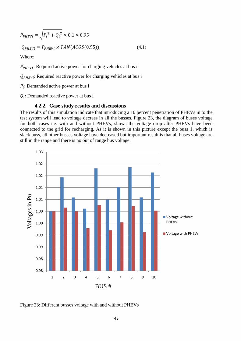
43

(4.1)

Where:

: Required active power for charging vehicles at bus i

: Required reactive power for charging vehicles at bus i

: Demanded active power at bus i

Demanded reactive power at bus i

4.2.2. Case study results and discussions

The results of this simulation indicate that introducing a 10 percent penetration of PHEVs in to the

test system will lead to voltage decrees in all the busses. Figure 23, the diagram of buses voltage

for both cases i.e. with and without PHEVs, shows the voltage drop after PHEVs have been

connected to the grid for recharging. As it is shown in this picture except the buss 1, which is

slack buss, all other busses voltage have decreased but important result is that all buses voltage are

still in the range and there is no out of range bus voltage.

Figure 23: Different busses voltage with and without PHEVs

0,98

0,98

0,99

0,99

1,00

1,00

1,01

1,01

1,02

1,02

1,03

1 2 3 4 5 6 7 8 9 10

Vo

ltag

es i

n P

u

BUS #

Voltage without PHEVs

Voltage with PHEVs

44

4.3. Effects of PHEVs on the 32-Bus Nordic system

While it is found the problems with low voltage distribution network mainly related to

overloading of distribution feeders, in the transmission level it was seen an interesting phenomena

caused by PHEVs on the 32-Bus Nordic system. The results have shown that with 10%

penetration level of PHEVs in this system, voltage levels at many buses have increased. This is

quite interesting since this is not normally the case for the radial system. It cannot be concluded

for all the system but for this particular Nordic 32-bus system, the power flows in the South have

changed significantly in the case with PHEVs as compared to the base case without PHEVs.

Nordic 32-bus system is a meshed transmission network with 3 voltage levels. The single-line

diagram of this system is shown in Fig. 9. The detailed information about the system can be found

in [14]. The test system information and assumptions that are considered for this case are as

below.

4.3.1. Description of Nordic 32-Bus system

Nordic 32-Bus system is a simulated Nordic transmission system. This network has got three

different voltage levels. Most of the generators have been located in the north part of the network

and most of the loads have been located in the south part. The power is transmitted from the north

part to the south part via the long transmission lines. Nordic 32-Bus system includes:

- 19 buses with 400 kV voltage, 2 busses of 220 kV and 20 busses of 130 kV.

- 20 generators.

- 22 loads.

- 11 switched shunts.

- 61 transmission lines.

22 other loads have been added to the system to simulate the PHEVs. Figure 24 shows an

overview of this network. In this figure the 400 kV busses and transmission lines have been shown

in black and 220 kV and 130 kV lines and busses are in gray. Again a power factor of 0.95 has

been considered for whole charging system i.e. battery and charging equipments. Required power

for charging PHEVs has been considered as a percentage of the present load. P and Q required for

charging at each bus is calculated according to equation (4.1).In the figure 25 required powers for

charging PHEVs have been shown with horizontal loads.

45

Figure 24: Nordic 32-Bus system overview

4.3.2. Case study results and description

To analyze effect of the PHEVs on the network, the following 3 cases have been considered:

- Business as usual (BAU): The system without PHEVs

- 10% penetration: The BAU with 10% load as PHEVs at each bus with load.

- 10% penetration V2G: The BAU with 10% load as V2G at each bus with load.

For simulation the V2G effect of the PHEVs on the transmission network, loads with minus sign

have been considered.

Introducing the penetration of 10 percent will dramatically change the voltage profile of the

transmission network. As shown in Table 16, figure 25 and 26, when adding PHEVs penetration

of 10% to the system, there would be 26 buses in the system with voltages level over the

maximum allowable limit. This is quite interesting since it is normally expected that the voltage is

decreased when the load is increased. However, this can always be true with the radial system like

in the distribution network. In the meshed network like the Nordic 32-bus system, when PHEVs

loads are added, the power flows over the system have changed quite significantly, especially the

reactive power flow. This makes the voltages magnitudes in southern part of the system increased.

In this simulation study, the increase in PHEVs load can be managed by existing generators for

both active and reactive power.

46

Figure 25: Nordic 32-Bus system with 10% penetration of PHEVs

Figure 26 shows a comparison between the voltage profile of the tests system before and after

introduction a penetration of PHEVs in to the transmission network.

47

Figure 26: Voltage profile of the system before and after introduction of 10% penetration of the

PHEVs

As it is seen in the figure 26, after adding PHEVs into the test system, almost all the network

voltages increase, meaning that power flow especially reactive power flow in the system has

changed dramatically.

Table 16: system specifications in three scenarios

No of over

voltage busses

No of under

voltage

busses

No of violations in N-1 contingency

analysis

Active

power

losses

Total active

power

generation

without PHEVs 0 0 307 violations and 9 unsolvable

contingencies 606.8 Mw 11679.8

with 10%

penetration of

PHEVS

26 1 1257 violations and 16 unsolvable

contingencies 964.6Mw 12544.9

with 10%

penetration of V2G 1 6 587 violations and 15 unsolvable

contingencies 491.5Mw 10254.3

Buss No 1041 is one of those buses which will have over voltage when there is a 10% penetration

of PHEVs .At this buss, it is possible to add 189.73 kVA load with PF of 0.95 lag for simulating

battery recharging while other busses are not serving PHEVs without reaching the overvoltage

limit. This amount of power is equivalent to normal charging of 124 PHEVs simultaneously. This

critical amount of load has been obtained by iterative method i.e. keep increasing the load at this

bus till bus voltage exceed the limit as it is illustrated in figure 27.

0,00

0,20

0,40

0,60

0,80

1,00

1,20

1,40

1,60

Vo

ltag

es in

PU

Bus #

BAU

with PHEVs

48

Figure 27: Iterative method for calculation maximum possible charging at one bus

Another important result from this study is that number of violations (mainly in bus voltages) in

N-1 contingency analysis of the system increases dramatically with 10% penetration of PHEVs,

indicating that power system security must be properly studied with mass introduction of PHEVs.

With V2G, the number of violations is reduced as compared to the 10% penetration of PHEVs

case. The number of violations in the 10% penetration of V2G is not less than the BAU scenario.

It can be concluded that when there is a V2G penetration, the number of existing elements in the

networks has increased and consequently the number of violations has increased. Table 16 also

shows a comparison between the losses in three scenarios. As it is observed, the minimum losses

are for the case with V2G penetration, which emphasizes the superior feature and economical

benefits of V2G.

Increase number of connected vehicle at bus

1041 while there are no other vehicles at all

other busses

Is bus voltage

in the

allowable

range?

This is the maximum possible

number of charging vehicles at bus

1041

Yes

No

49

Chapter 5

5. Maximizing penetration of DGs in the distribution network

5.1. Over voltage effect of the DGs in the networks and introduction of the existing

solutions

Uropean governments are working toward an ambitious target of considerably increasing the

amount of the renewable energy in order to reduce the adverse environmental impacts of

traditional sources of energy [15] and [16].The superior feature of using green energy

sources encourage the governments all around the world to keep on investment on the renewable

energy sources. This new tendency toward green energy sources has arisen many challenges

regarding embedded generation. The connection of DGs, their protection and also their operation

in the different load levels are new challenges that have been posed to the power system operators.

These challenges usually limit the penetration level of DGs to the existing network. For example

in a rural network, voltage rise effect is a factor that limits the penetration of the wind turbine or

DGs in general. To overcome the voltage rise effect, power system operators prefer to connect the

wind turbines to the high voltage side to minimize the effect of voltage rise but the economical

viability of the wind turbine is very sensitive to connection costs i.e. the higher the voltage the

higher the costs and therefore the developers of the wind turbines prefer to connect at lower

voltage [15]. At time being, there are three ways for mitigation voltage rise effect in the networks

equipped with DGs.

- Power curtailment, which means decrees the power output of the distributed generator

when it is lightly loaded.

- Absorbing reactive power at DGs bus can mitigate the voltage rise effect. So using of

reactive power control facilities like STATCOM at connecting point is recommended.

- Using of co-ordinated voltage control strategy for example by OLTC (On load tap

changer) is another existing solution for voltage rise effect.

5.2. Over voltage effect of DGs on the modified IEEE 13 –Node test distribution

systems

To study the voltage rise effects in the networks equipped with DGs, one sample network

including three distributed generators has been tested and possible solution for mitigation of over

voltage has been simulated. The test network is IEEE13-Node test distribution system. It has been

E

50

modified to fit in our simulation. The single phase loads has changed to three phase loads to make

the Power World simulation possible. Figure 28 shows how this test system looks like.

Figure 28: Over view of the IEEE 13- Node test system with some modification.

5.2.1. Description of modified IEEE 13 –Node test distribution systems.

System which has been used for this study is IEEE 13-Node test system. It has been modified to

fit in our investigation. The impedance of all three phases in the cables and over headlines are

equal. The imbalanced loads have changed to balanced loads to be able to simulate the network

with Power World. Three generators have been added to this system at busses 645,671 and 675.

These generators show the DGs in the distribution network. The line ambacities have been set

according to [8].

These systems include:

- 13 busses with voltages of 115KV, 4.16KV and 0.48 KV.

- 9 loads

- 2 transformers.

- 2 capacitors at bus 611 and 675.

- 3 distributed generators and one slack generator

Bus number 693 has been added just for connecting transformer to the line.

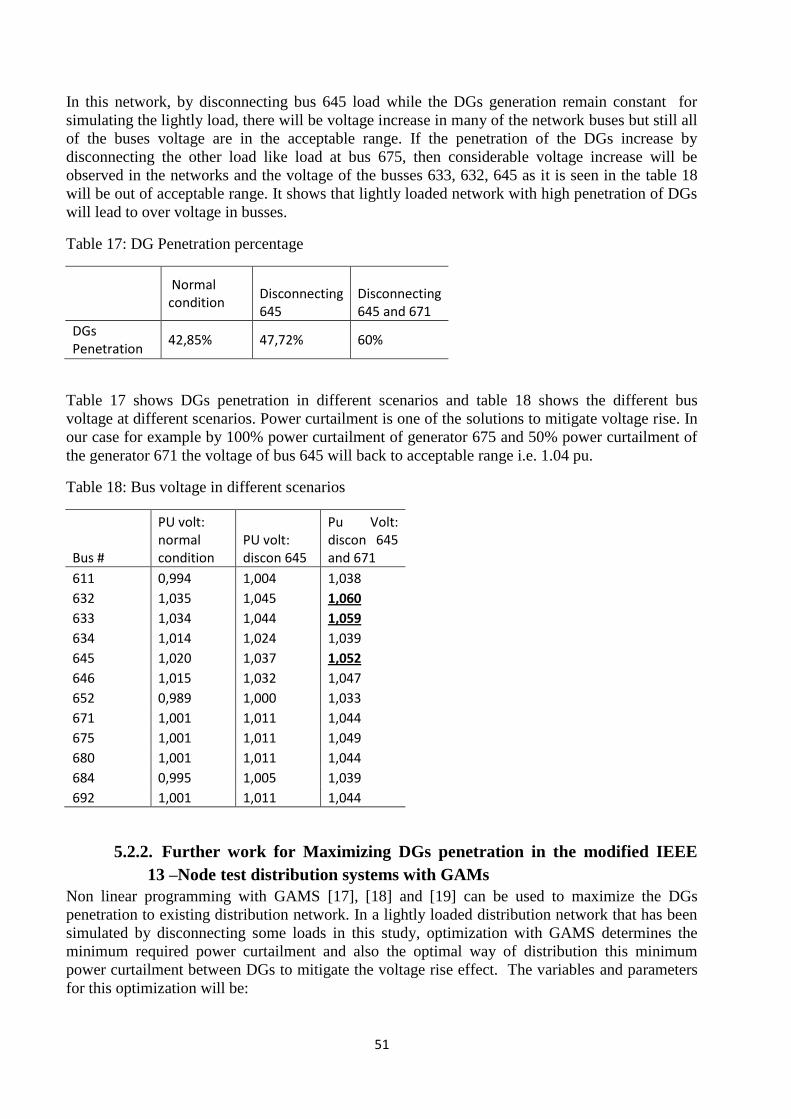
51

In this network, by disconnecting bus 645 load while the DGs generation remain constant for

simulating the lightly load, there will be voltage increase in many of the network buses but still all

of the buses voltage are in the acceptable range. If the penetration of the DGs increase by

disconnecting the other load like load at bus 675, then considerable voltage increase will be

observed in the networks and the voltage of the busses 633, 632, 645 as it is seen in the table 18

will be out of acceptable range. It shows that lightly loaded network with high penetration of DGs

will lead to over voltage in busses.

Table 17: DG Penetration percentage

Normal condition

Disconnecting 645

Disconnecting 645 and 671

DGs Penetration

42,85% 47,72% 60%

Table 17 shows DGs penetration in different scenarios and table 18 shows the different bus

voltage at different scenarios. Power curtailment is one of the solutions to mitigate voltage rise. In

our case for example by 100% power curtailment of generator 675 and 50% power curtailment of

the generator 671 the voltage of bus 645 will back to acceptable range i.e. 1.04 pu.

Table 18: Bus voltage in different scenarios

Bus #

PU volt: normal condition

PU volt: discon 645

Pu Volt: discon 645 and 671

611 0,994 1,004 1,038

632 1,035 1,045 1,060

633 1,034 1,044 1,059

634 1,014 1,024 1,039

645 1,020 1,037 1,052

646 1,015 1,032 1,047

652 0,989 1,000 1,033

671 1,001 1,011 1,044

675 1,001 1,011 1,049

680 1,001 1,011 1,044

684 0,995 1,005 1,039

692 1,001 1,011 1,044

5.2.2. Further work for Maximizing DGs penetration in the modified IEEE

13 –Node test distribution systems with GAMs

Non linear programming with GAMS [17], [18] and [19] can be used to maximize the DGs

penetration to existing distribution network. In a lightly loaded distribution network that has been

simulated by disconnecting some loads in this study, optimization with GAMS determines the

minimum required power curtailment and also the optimal way of distribution this minimum

power curtailment between DGs to mitigate the voltage rise effect. The variables and parameters

for this optimization will be:

52

i subscript for all of the buses

j subscript for all of the buses

k subscript for the DG buses

Pi generation power at bus i

Pdemi demand power at each bus

Q i generation power at bus i

Qdemi demand power at bus i

V i voltage amplitude at bus i

Deltai voltage angle at bus i

Pcuri curtailed power at bus i which is set to zero for non DG busses and has been

limited between zero and maximum power of DG at DG busses.

Genphii DGs generation angle i.e. ARCTAN (Q/P) for DGs buses and is zero for all the other

buses.

Y (i,j) admittance amplitude between bus i and j

Theta (i,j) admittance angle between bus i and j

Penet summation of DGs generation minus summation of DGs curtailment

Objective function is maximizing Penet= (5.1)

Constraint 1 for all the buses will be active power flow equation:

(5.2)

And constraint 2 for all the buses will be reactive power flow equation:

(5.3)

Total program text is available in the Appendix A.

53

Chapter 6

6. Conclusions

6.1. Conclusions

his master thesis summarizes possible key effects of introduction of PHEVs in the power

system. Results from the studies on the IEEE 13-Node test system, show that problems with

low voltage distribution networks with PHEVs are mainly related to overloading of

distribution feeders, and under voltages in end-users locations, in the case of quick charging

during peak load period. If normal charging is to be used, the system would be able to support the

PHEVs without overloading and under voltage problems.

Study on the real distribution network in the Gothenburg indicates that if charging of vehicles,

with most probable distribution which is proportional to loads, left uncontrolled overloading of

lines at peak load in the 10 kV network will happen and it implies requirement for smart charging

strategy. Study results show that if there is suitable voltage controller in the 10 kV network i.e.

main supplier busbar in the 10 kV network has voltage higher than1 pu, the voltage drop in the

400 V network will be negligible both for the commercial and residential area. Fuse rating of the

main feeders for the customers in the residential and commercial area must be revised if one phase

plug is used for charging the vehicles. Introduced procedure for calculation maximum possible

charging in one area can be useful to give an over view of distribution network capacity for

charging vehicles in the secure manner to the system operators.

In the transmission level, effects of vehicles charging on the network are strongly dependent to

the network topology. While in the 10-Bus test system, voltage drop was the result of PHEVS

penetration, an interesting phenomenon with regard to the bus voltage level is observed for the

Nordic 32-bus system. That is when PHEVs equally distributed in the system; the voltage in the

system might increase, showing the need for voltage regulation measures. However, this could not

be concluded for every system since this is system-dependent. Another problem with meshed

transmission networks is typically that the level of security could be affected when more PHEVs

are plugged into the network.

In the last chapter, study results show the necessity of mitigating measurers regarding with the

voltage rise effect in the distribution networks equipped with Distributed Generators. It was also

proposed to use the Nonlinear programming with GAMS for maximizing DGs penetration in the

lightly loaded situation.

T

54

6.2. Future research directions

The following topics which are relevant to the current work are proposed for the further work.

- Since most of the quantities related to effects of PHEVs on the power systems topic are

probabilistic quantities, so one comprehensive statistic research about the people driving

behavior in the under research area is required.

- Many of the research relates to PHEVs effects on the power system, have concluded that

one smart charging strategy is required, therefore in each area many research and

investigation are required to find an optimal charging strategy

- A dynamic model of all kind of the electric vehicles is required to investigate the effect of

these vehicles on the power systems stability in the transient states.

- Protective scheme of the distribution systems with mass introduction of PHEVs must be

revised and especially in the case that these vehicles are capable of power injection to grid

this revision will be more necessary.

- Precise model of the DGs in the GAMS will improve the optimal penetration of the DGs in

the existing distribution networks.

55

7. Appendix A Text of the optimization program with GAMS.

**********************************************************************************

set i buses/611,632,633,634,645,646,650,652,671,675,680,684,692,693/ ;

alias (i,j);

set k(i) DGs/645,671,675/;

set f(i) non DG Busses /611,632,633,634,646,650,652,680,684,692,693/

load(i) Load buses /611,632,633,634,645,646,652,671,675,680,684,692,693/

Head1 Generator data headings / PMin, PMax, QMin, QMax, A, B, C, D, E, F/

Head2 Line data table headings / Re, Xe, Ch /

Head3 Demand data table headings / PDem, QDem /;

Scalar Base base KVA /100000 /;

scalar phi /3.141592654 /;

************************** DATA SECTION ****************************************

TABLE Generation(i,Head1) generator data

PMin PMax QMin QMax A B C

* KW KW KVAR KVAR

*645 0 230 0 75.593 1.0 8.50 5

650 0 3100 -1000 3100 3.4 25.50 9

*671 0 1000 -100 328.66 3.4 25.50 9

*675 0 750 -100 846.5 3.4 25.50 9

*611 0 0 0 100

;

*****------- Convert generator data to per unit quantities ----------*******

Parameter PMx(i), PMn(i), QMx(i), QMn(i), Ac(i), Bc(i), Cc(i),SMaxpu;

PMx(i) = Generation(i,"PMax")/Base;

PMn(i) = Generation(i,"PMin")/Base;

QMx(i) = Generation(i,"QMax")/Base;

QMn(i) = Generation(i,"QMin")/Base;

Ac(i) = Generation(i,"A")*Base*Base;

Bc(i) = Generation(i,"B")*Base;

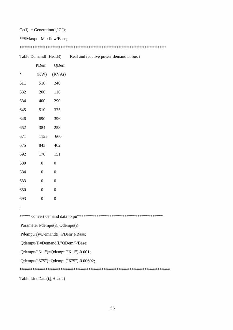
56

Cc(i) = Generation(i,"C");

**SMaxpu=Maxflow/Base;

********************************************************************

Table Demand(i,Head3) Real and reactive power demand at bus i

PDem QDem

* (KW) (KVAr)

611 510 240

632 200 116

634 400 290

645 510 375

646 690 396

652 384 258

671 1155 660

675 843 462

692 170 151

680 0 0

684 0 0

633 0 0

650 0 0

693 0 0

;

***** convert demand data to pu****************************************

Parameter Pdempu(i), Qdempu(i);

Pdempu(i)=Demand(i,"PDem")/Base;

Qdempu(i)=Demand(i,"QDem")/Base;

Qdempu("611")=Qdempu("611")-0.001;

Qdempu("675")=Qdempu("675")-0.00602;

**********************************************************************

Table LineData(i,j,Head2)

57

Re Xe Ch

* (p.u.) (p.u.) (p.u.)

632.645 0.7261 0.7358 0

632.633 0.0863 0.2313 0

633.634 2.2 4 0

645.646 0.4357 0.4415 0

650.693 0.1 0.8 0

693.632 0.37 1.1 0

684.652 1.173 0.4478 0

632.671 0.7570 2.2240 0

671.684 0.4326 0.4447 0

671.680 0.3785 1.1120 0

671.692 0 0 0

684.611 0.1135 0.3336 0

692.675 0.4360 0.2798 0

;

*---FORMATION OF THE Y-BUS MATRIX ------------------------------------

Parameter Z(i,j), GG(i,j), BB(i,j), YCL(i);

Parameter G(i,j), B(i,j), Y(i,j), ZI(i,j), Theta(i,j);

LineData(j,i,"Re")$(LineData(i,j,"Re") gt 0.00) = LineData(i,j,"Re");

LineData(j,i,"Xe")$(LineData(i,j,"Xe") gt 0.00) = LineData(i,j,"Xe");

LineData(j,i,"Ch")$(LineData(i,j,"Ch") gt 0.00) = LineData(i,j,"Ch");

Z(i,j) = (LineData(i,j,"Re"))**2 + (LineData(i,j,"Xe"))**2 ;

GG(i,j)$(Z(i,j) ne 0.00) = LineData(i,j,"Re")/z(i,j) ;

BB(i,j)$(Z(i,j) ne 0.00) = -LineData(i,j,"Xe")/Z(i,j);

BB(j,i)$(Z(i,j) ne 0.00) = -LineData(i,j,"Xe")/Z(i,j);

YCL(i) = sum(j, LineData(i,j,"Ch"));

B(i,i) = sum(j, BB(i,j)) + YCL(i);

G(i,i) = sum(j, GG(i,j));

G(i,j)$(ord(i) ne ord(j)) = -GG(i,j);

B(i,j)$(ord(i) ne ord(j)) = -BB(i,j);

58

Y(i,j) = sqrt(G(i,j)*G(i,j) + B(i,j)*B(i,j));

ZI(i,j)$(G(i,j) ne 0.00) = abs(B(i,j))/abs(G(i,j)) ;

Theta(i,j) = arctan(ZI(i,j));

Theta(i,j)$((B(i,j) eq 0) and (G(i,j) gt 0)) = 0.0 ;

Theta(i,j)$((B(i,j) eq 0) and (G(i,j) lt 0)) = -0.5*phi ;

Theta(i,j)$((B(i,j) gt 0) and (G(i,j) gt 0)) = Theta(i,j) ;

Theta(i,j)$((B(i,j) lt 0) and (G(i,j) gt 0)) = 2*phi - Theta(i,j) ;

Theta(i,j)$((B(i,j) gt 0) and (G(i,j) lt 0)) = phi - Theta(i,j);

Theta(i,j)$((B(i,j) lt 0) and (G(i,j) lt 0)) = phi + Theta(i,j);

Theta(i,j)$((B(i,j) gt 0) and (G(i,j) eq 0)) = 0.5*phi;

Theta(i,j)$((B(i,j) lt 0) and (G(i,j) eq 0)) = -0.5*phi;

Theta(i,j)$((B(i,j) eq 0) and (G(i,j) eq 0)) = 0.0 ;

******************* Variable Declaration *****************************

positive variable V(i) the bus voltage amplitude;

free variable Delta(i) the bus voltage phase;

free variable P(i) the bus active power generation;

free variable Q(i) the bus reactive power generation;

free variable Pcur(i) the curtailed active power of the DGs;

free variable loss the total loss;

integer variable T position of the tap changer of the DG at bus # 650;

free variable S(i,j) the amplitude of apparent power between the buss i and j;

free variable Penet penetration of the DGs;

********** *************Initialization of variables*************************************

V.l(i)=1;

V.fx("650")=1.1;

Delta.l(i)=0;

Delta.fx("650")=0;

P.up(i)=PMx(i);

P.lo(i)=PMn(i);

Q.up(i)=QMx(i);

Q.lo(i)=QMn(i);

59

P.fx("645")=0.003;

P.fx("671")=0.01;

P.fx("675")=0.008;

Q.fx("645")=-0.00432;

Q.fx("671")=0.00028;

Q.fx("675")=-0.0007;

********************DGs Power factor definition***************************************

Parameter genphi(i) the angle of the generators ;

genphi("611")=0;

genphi("632")=0;

genphi("634")=0;

genphi("646")=0;

genphi("650")=0;

genphi("652")=0;

genphi("680")=0;

genphi("684")=0;

genphi("692")=0;

genphi("693")=0;

genphi("633")=0;

genphi("645")=arctan(Q.l("645")/P.l("645"));

genphi("671")=arctan(Q.l("671")/P.l("671"));

genphi("675")=arctan(Q.l("675")/P.l("675"));

Pcur.up("675")=P.l("675");

Pcur.lo("675")=0;

Pcur.up("671")=P.l("671");

Pcur.lo("671")=0;

Pcur.up("645")=P.l("645");

Pcur.lo("645")=0;

*Pcur.fx("645")=0;

*Pcur.fx("671")=0;

*Pcur.fx("675")=0;

60

Pcur.fx("611")=0;

Pcur.fx("632")=0;

Pcur.fx("633")=0;

Pcur.fx("634")=0;

Pcur.fx("646")=0;

Pcur.fx("650")=0;

Pcur.fx("652")=0;

Pcur.fx("680")=0;

Pcur.fx("684")=0;

Pcur.fx("692")=0;

Pcur.fx("693")=0;

*****************************Assignment of the Bounds**************************

V.lo(load)=0.95;

V.up(load)=1.05;

***************** ****definition of equations******************************************

Equation

obj

*LOSSES

const1(i)

const2(i);

obj..

Penet=e=sum(k,P(k))-sum(k,Pcur(k));

*LOSSES..

*Loss =e= 0.5*SUM( (i,j) , (-1)*G(i,j)*( V(i)*V(i) + V(j)*V(j) - ( 2*V(i)*V(j)*cos( Delta(j)-Delta(i) ) ) )

);

const1(i)..

P(i)=e=Pdempu(i)+Pcur(i)+sum(j,V(i)*V(j)*Y(i,j)*cos(Theta(i,j)+Delta(j)-Delta(i)));

const2(i)..

Q(i)=e=Qdempu(i)+(Pcur(i)*(sin(genphi(i))/cos(genphi(i))))-

sum(j,V(i)*V(j)*Y(i,j)*sin(Theta(i,j)+Delta(j)-Delta(i)));

model OPF/all/;

SOLVE OPF using NLP maximizing Penet;

61

DISPLAY P.l ;

DISPLAY Q.l ;

Display Penet.l;

DISPLAY v.l;

Display Pcur.l;

Display Delta.l;

Display P.lo;

Display P.up;

62

8. Appendix B

EEFFFFEECCTTSS OOFF PPHHEEVVss IINN PPOOWWEERR DDIISSTTRRIIBBUUTTIIOONN SSYYSSTTEEMMSS:: RREEVVIIEEWWSS AANNDD

AANNAALLYYSSEESS Saman BABAEI Tuan LE Lina BERTLING Ola CARLSON

Chalmers University of Technology, 41296 Gothenburg, Sweden

samanb@student.chalmers.se, tuan.le@chalmers.se, lina.bertling@chalmers.se, ola.carlson@chalmers.se

ABSTRACT

This paper deals with the analysis of the impacts of plug-

in hybrid electric vehicles (PHEVs) on the power system,

with focus on the low voltage power distribution system.

First a review of the technical challenges in the power

system due to the mass introduction of PHEVs in the

transporation sector is given. Then the paper shows on an

analysis of the overloading effects of PHEVs on the

distribution system with normal charging and quick

charging of PHEVs for an IEEE 13-node distribution test

system using power flow analysis. The results of the study

show that introduction of PHEVs in the transportation

sector will lead to overloading of distribution system and

cause voltage problems at the end-users. The paper also

analyzes the effects of PHEVs in the transmission system,

using the Nordic 32-bus test system. The study results

showed that the overloading problem is not prominent.

However, one interesting and important result is that

PHEVs may lead to overvoltages in some buses in the

transmission system which requires the voltage control

measures. PHEVs would also lead to increased number of

network violations in the contingency analysis.

Introduction

High penetration of plug-in hybrid electric vehicles

(PHEVs) in the transportation sector will likely be

envisioned by the transportation authority as well as energy

authority in many parts of the world, e.g., European

countries, Japan, and the USA. The benefits from replacing

the conventional internal combustion vehicles by the

PHEVs are the subjects of many current research and mass-

media because the transport sector is one of the largest and

fastest growing contributors to energy demand, urban air

pollution, and greenhouse gases (GHGs) [1]. The

possibility to reduce the dependency on oil consumption by

the transportation sector and the possibility to reduce

harmful environmental emissions, e.g., CO2, SOx, and NOx

by ways of improved conversion efficiency through PHEVs

are the key socio-economical and environmental benefits.

Given the said benefits, critics have warned that the

vehicles could put too much pressure on already strained

power grids. The concern is that plug-ins may not appear to

be a good way to reduce gasoline consumption, because if

they become popular, and millions of car owners recharged

their cars at three in the afternoon on a hot day, it would

crash the grid. Specially, uncontrolled charging can lead to

grid problem on the local scale [2].

The organization of the paper is as follows: The next

section will provide a brief overview and discussions on

the effects of PHEVs on the power system with focus on

the low voltage power distribution system. The power

flow analysis in the IEEE test distribution system when

assuming certain levels of PHEVs penetration levels is

presented in the following section. The effects on PHEVs

on the meshed transmission network are shown in the

following section. The grid support effects of PHEVs are

also analyzed through the contingency analysis of the

transmission system. Finally, conclusions and remarks are

made in the last section.

PHEVs in the power DISTRIBUtion sytem: A brief review As highlighted in the previous section, PHEVs have the potentials to contribute to reduce the environmental emissions from the transportation sector. However, it will likely pose new challenges in the power system, especially in the power distribution system where the vehicles are directly connected to. This section will highlight those challenges and effects. Other detailed information about the current technology and charging requirement of PHEVs will be presented in the next Section. Fig. 1 shows the effects of PHEVs on the power systems, and categorizes the problems at different levels, i.e., at system level, distribution system level, and transmission system level. The key question being asked today is how the power system sees the increase in its total loads when high level of PHEVs will be used in the near future. This is largely dependent on the charging habits which will be practiced by the users of PHEVs. As shown in Fig. 1, even though the PHEVs are connected in low voltage distribution system, they also have large effects on the generation system and transmission system levels. If the vehicle users are free to charge their cars anytime they want (uncontrolled charging), one can easily say that they will plug in at the end of the day, which corresponds with peak loads. In this case, PHEV increases the system peak loads which require additional generation (and transmission) capacity. A new dimension of peak load capacity for the power system might be required if the charging of PHEV is left uncontrolled. On the other hand, if controlled charging is used, which means that the utility controls charging between, for example, 10:00 pm and 07:00 am. In this case the system load profile will be improved in a way similar to the effect of “valley filling” demand-side management measure, meaning that the system utilization can be improved. PHEVs would result in the changes in the system load shapes which in turn would result in changes in power

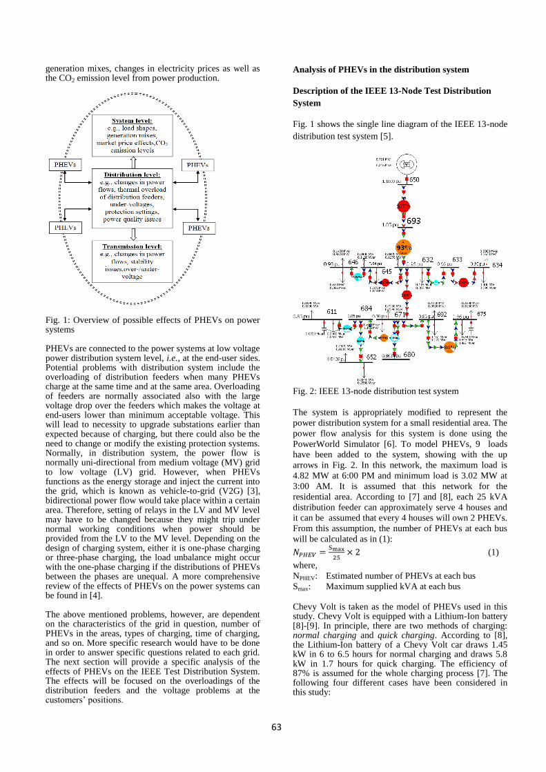
63

generation mixes, changes in electricity prices as well as the CO2 emission level from power production.

Fig. 1: Overview of possible effects of PHEVs on power systems PHEVs are connected to the power systems at low voltage power distribution system level, i.e., at the end-user sides. Potential problems with distribution system include the overloading of distribution feeders when many PHEVs charge at the same time and at the same area. Overloading of feeders are normally associated also with the large voltage drop over the feeders which makes the voltage at end-users lower than minimum acceptable voltage. This will lead to necessity to upgrade substations earlier than expected because of charging, but there could also be the need to change or modify the existing protection systems. Normally, in distribution system, the power flow is normally uni-directional from medium voltage (MV) grid to low voltage (LV) grid. However, when PHEVs functions as the energy storage and inject the current into the grid, which is known as vehicle-to-grid (V2G) [3], bidirectional power flow would take place within a certain area. Therefore, setting of relays in the LV and MV level may have to be changed because they might trip under normal working conditions when power should be provided from the LV to the MV level. Depending on the design of charging system, either it is one-phase charging or three-phase charging, the load unbalance might occur with the one-phase charging if the distributions of PHEVs between the phases are unequal. A more comprehensive review of the effects of PHEVs on the power systems can be found in [4]. The above mentioned problems, however, are dependent on the characteristics of the grid in question, number of PHEVs in the areas, types of charging, time of charging, and so on. More specific research would have to be done in order to answer specific questions related to each grid. The next section will provide a specific analysis of the effects of PHEVs on the IEEE Test Distribution System. The effects will be focused on the overloadings of the distribution feeders and the voltage problems at the customers’ positions.

Analysis of PHEVs in the distribution system

Description of the IEEE 13-Node Test Distribution

System

Fig. 1 shows the single line diagram of the IEEE 13-node

distribution test system [5].

Fig. 2: IEEE 13-node distribution test system

The system is appropriately modified to represent the

power distribution system for a small residential area. The

power flow analysis for this system is done using the

PowerWorld Simulator [6]. To model PHEVs, 9 loads

have been added to the system, showing with the up

arrows in Fig. 2. In this network, the maximum load is

4.82 MW at 6:00 PM and minimum load is 3.02 MW at

3:00 AM. It is assumed that this network for the

residential area. According to [7] and [8], each 25 kVA

distribution feeder can approximately serve 4 houses and

it can be assumed that every 4 houses will own 2 PHEVs.

From this assumption, the number of PHEVs at each bus

will be calculated as in (1):

(1)

where,

NPHEV: Estimated number of PHEVs at each bus

Smax: Maximum supplied kVA at each bus

Chevy Volt is taken as the model of PHEVs used in this study. Chevy Volt is equipped with a Lithium-Ion battery [8]-[9]. In principle, there are two methods of charging: normal charging and quick charging. According to [8], the Lithium-Ion battery of a Chevy Volt car draws 1.45 kW in 6 to 6.5 hours for normal charging and draws 5.8 kW in 1.7 hours for quick charging. The efficiency of 87% is assumed for the whole charging process [7]. The following four different cases have been considered in this study:

64

1. Business as usual (BAU): System at peak load

without PHEVs.

2. Normal charging, peak load: BAU with PHEVs

normal charging

3. Quick charging, peak load: BAU with PHEVs quick

charging

4. Quick charging, min load: System at min load with

PHEVs quick charging

Case study results and discussions

Tables 1 shows the bus voltages of four different

scenarios described above. In the BAU case, all the bus

voltages are within the acceptable limits of ±10% of

nominal voltage. In the normal charging case, there were

no violations in voltages at all the buses. However, in the

quick charging at peak load scenarios, there are 50% of

buses with voltage below the minimum acceptable level

(shown with underlined numbers in Table 1). It is because

that quick charging draws much higher current/power

than the normal charging. The voltages at different buses

in the case of quick charging at max load are also shown

in Fig. 2 above. If quick charging can be controlled and

done during the min load period, there were no problem

of voltage violations in the system as shown in Table 1.

Table 1: Buses voltages in per unit for different scenarios

Bus # BAU

Normal

charging, peak load

Quick

charging, peak load

Quick

charging, min load

611 0.97 0.95 0.85 0.96

632 1.03 1.01 0.96 1.02

633 1.03 1.01 0.96 1.02 634 1.00 0.99 0.93 1.00

645 1.01 1.00 0.94 1.00

646 1.01 0.99 0.93 1.00 650 1.10 1.10 1.10 1.10

652 0.96 0.94 0.84 0.95

671 0.97 0.95 0.86 0.97 675 0.97 0.95 0.86 0.96

680 0.97 0.95 0.86 0.97

684 0.97 0.95 0.85 0.96 692 0.97 0.95 0.86 0.97

693 1.07 1.07 1.05 1.07

Table 2 shows the line loadings in percentage of rated line

capacity. In the BAU and normal charging scenarios, the

line loadings are within the maximum limits.

Table 2: Loading of lines as percentage of rated power

From

bus

To

bus BAU

Normal charging,

peak load

Quick charging,

peak load

Quick charging,

min load

684 611 32.20 37.10 51.80 39.00 632 633 20.70 23.60 32.60 25.00

632 645 87.50 99.80 137.80 106.00

632 671 66.20 75.90 113.70 80.90 693 632 56.20 64.90 97.50 68.80

633 634 67.20 76.60 105.80 81.20

645 646 48.40 55.20 75.70 58.60 650 693 60.50 70.10 107.40 74.20

684 652 38.80 44.10 60.40 45.70

671 680 0.00 0.00 0.00 0.00 671 684 60.00 69.00 96.60 72.30

671 692 0.00 0.00 0.00 0.00

675 692 45.60 52.20 73.90 57.50

When PHEVs are charged with quick charging during

peak load period, there are four lines (i.e., lines 632-645,

632-671, 633-634, and 650-693) overloaded as can be

seen with the red circles in Fig. 2, meaning that the

network is under the stress condition. With quick

charging but under the min load condition, the stress

condition for the line overloading is reduced with only

one line overloading (i.e., line 632-645).

Fig. 3 shows total system active power losses for different

scenarios. System loss increases dramatically when

PHEVs have been connected for quick charging at peak

load as compared to the BAU scenario. Total system

losses at normal charging at peak load and quick charging

at minimum load are found to be the same.

Fig. 3: Total system active power losses

As shown in Fig. 1 and discussed in previous section,

PHEVs are connected directly in the distribution network

but they will have potential effects in the meshed

transmission network. The following section will present

the power flow analysis for the effects of PHEVs on the

Nordic 32-bus test system.

Analysis of PHEVs in the meshed Transmission

network

The Description of Nordic 32-Bus System

Nordic 32-bus system is used in this study to represent

different scenarios with PHEVs. The single-line diagram

of this system is shown in Fig. 4. The detailed

information about the system can be found in [10]. In this

study, 22 loads have been added to the network to

represent PHEVs load. The PHEVs penetration has been

considered as percent of total load of each bus with load

connected in the system. Batteries have been modelled

with negative loads when they are injecting power into

the grid (i.e, in V2G mode). To analyse the effect of the

PHEVs on the network, the following 3 cases have been

considered:

1. Business as usual (BAU): The system without

PHEVs

2. 10% penetration: The BAU with 10% load as

PHEVs at each bus with load.

3. 10% penetration V2G: The BAU with 10% load as

V2G at each bus with load.

65

Fig. 4: Single line diagram of Nordic 32-bus system

Case study results and discussions

Introducing the penetration of 10 percent will dramatically change the voltage profile of the transmission network. As shown in Table 3, when adding PHEVs penetration of 10% to the system, there would be 26 buses in the system with voltages level over the maximum allowable limit. This is quite interesting since it is normally expected that the voltage is decreased when the load is increased. However, this can always be true with the radial system like in the distribution network. In the meshed network like the Nordic 32-bus system, when PHEVs loads are added, the power flows over the system have changed quite significantly, especially the reactive power flow. This makes the voltages magnitudes in southern part of the system increased. In this simulation study, the increase in PHEVs load can be managed by existing generators for both active and reactive power.

Table 3: Case study results for 3 cases

No of

over voltage

buses

No of

under voltage

buses

No of violations in N-1 contingency analysis

BAU 0 0 307 violations and 9 unsolvable contingencies

10% penetration of

PHEVs

26 1 1257 violations and 16

unsolvable contingencies

with 10% penetration of

V2G

1 6 587 violations and 15

unsolvable contingencies

Another important result from this study is that the number of violations (mainly in bus voltages) in N-1 contingency analysis of the system increases dramatically with 10% penetration of PHEVs, indicating that power system security must be properly studied with mass introduction of PHEVs. With V2G, the number of violations is reduced as compared to the 10% peneration of PHEVs case.

conclusion

This paper summarizes possible key effects of

introduction of PHEVs in the power system. Results from

the studies show that problems with low voltage

distribution networks with PHEVs are mainly related to

overloadings of distribution feeders, and under voltages in

end-users’ locations in the case of quick charging during

peak load period. If normal charging is to be used, the

system would be able to support the PHEVs without

overloading and under voltage problems. In the

transmission level, an interesting phenomena with regard

to the bus voltage level is observed for the Nordic 32-bus

system. That is when PHEVs equally distributed in the

system, the voltage in the system might increase, showing

the need for voltage regulation measures. However, this

could not be concluded for every system since this is

system-dependent. An other problem with meshed

transmission networks is typically that the level of

security could be affected when more PHEVs are plugged

into the network.

REFERENCES

[1] A. Hajimiragha, C.A. Cañizares, M.W. Fowler, and

A. Elkamel, 2010, "Optimal transition to Plug-In

Hybrid Electric Vehicles Ontario, Canada;

considering the electricity- grid limitations", IEEE

Transactions on Industrial Electronics, Vol. 57, NO.

2.

[2] K.C. Nyns, E. Haesen, and J. Driesen, 2010, "The

impact of charging Plug-In Hybrid Electric Vehicle

on a residential distribution grid", IEEE Transaction

Power Systems, Vol. 25, No. 1.

[3] W. Kempton, V. Udo, K Huber, K Komara, S

Letendre, S. Baker, D. Brunner, N. Pearre, 2008, "A

test of Vehicle-to-Grid (V2G) for energy storage and

frequency regulation in the PJM System". Available

http://www.magicconsortium.org/_Media/test-v2g-

in-pjm-jan09.pdf

[4] S. Haghbin, T. Le, A. Lindskog, S. Lundmark, 2009,

“State of the art of Plug-in Hybrid Electric Vehicles”,

Tehnical report, Chalmers University of Technology.

[5] W.H. Kersting, 2001, “Radial distribution test

feeders”, Power Engineering Society Winter Meeting,

Vol. 2, 908 – 912.

[6] PowerWorld Corporation,

http://www.powerworld.com/

[7] K. Schneider, C. Gerkensmeyer, M. Kintner-Meyer,

and R. Fletcher, 2008, "Impact assessment of Plug-In

Hybrid Vehicles on pacific northwest distribution

systems", IEEE Power and Energy Society General

Meeting-Conversion and Delivery of Electrical

Energy.

[8] S. Shao, M. Pipattanasomporn, and R. Saifur, 2009,

"Challenges of PHEV penetration to the residential

distribution network", IEEE Power and Energy

Society General Meeting

[9] Chevy Volt website. Available http://www.chevy-

volt.net/chevrolet-volt-specs.htm

[10] CIGRE TF 38-02-08, "Long Term Dynamics Phase

II", 1995.

66

9. Bibliography

[1]. Hajimiragha, C.A. Cañizares, M.W. Fowler, and A. Elkamel, 2010, "Optimal transition to

Plug-In Hybrid Electric Vehicles Ontario, Canada; considering the electricity- grid

limitations", IEEE Transactions on Industrial Electronics, Vol. 57, NO. 2

[2]. K.C. Nyns, E. Haesen, and J. Driesen, 2010, "The impact of charging Plug-In Hybrid Electric

Vehicle on a residential distribution grid", IEEE Transaction Power Systems, Vol. 25, No. 1.

[3]. W. Kempton, V. Udo, K Huber, K Komara, S Letendre, S. Baker, D. Brunner, N. Pearre,

2008, "A test of Vehicle-to-Grid (V2G) for energy storage and frequency regulation in the

PJM System". Available http://www.magicconsortium.org/_Media/test-v2g-in-pjm-jan09.pdf

[4]. Trishna Das, Dionysios C. Aliprantis, 2008, "Small-Signal Stability Analysis of Power

System Integrated with PHEVs", Energy 2030 Conference

[5]. S. De Breucker, P. Jacqmer, K. De Brabandere, J. Driesen, and R.Belmans, 2006, "Grid

power quality improvements using grid-coupled hybrid electric vehicles", Power Electronics,

Machines, and Drives, pp. 505-509.

[6]. PowerWorld Corporation, http://www.powerworld.com/

[7]. S. Haghbin, T. Le, A. Lindskog, S. Lundmark, 2009, “State of the art of Plug-in Hybrid

Electric Vehicles”, Tehnical report, Chalmers University of Technology

[8]. W.H. Kersting, 2001, “Radial distribution test feeders”, Power Engineering Society Winter

Meeting, Vol. 2, 908 – 912.

[9]. S.D. Jenkins, J.R.Rossmaier, and M. Ferdowsi, 2008, " Utilization and effect of Plug-In hybrid

electric vehicles in the United States power grid", IEEE Vehicle Powerand Propulsion

Conference.

[10]. K. Schneider, C. Gerkensmeyer, M. Kintner-Meyer, and R. Fletcher, 2008, "Impact

assessment of Plug-In Hybrid Vehicles on pacific northwest distribution systems", IEEE

Power and Energy Society General Meeting-Conversion and Delivery of Electrical Energy.

[11]. S. Shao, M. Pipattanasomporn, and R. Saifur, 2009, "Challenges of PHEV penetration to

the residential distribution network", IEEE Power and Energy Society General Meeting

[12]. Chevy Volt website. Available http://www.chevy-volt.net/chevrolet-volt-specs.htm

[13]. D. Steen, 2010, "Report on Plug-in vehicles"

[14]. CIGRE TF 38-02-08, "Long Term Dynamics Phase II", 1995.

[15]. S.N. Liew, G. Strbac,2002, "Maximising penetration of wind generation in existing

distribution network", IEE proceeding online no 20020218.

[16]. L.F. Ochoa, L.C. Cradden, and G.P. Harrison,20101, " Demonstrating the capacity benefits

of dynamic rating in smarter distribution network ", IEEE Inovative Smart Grid Technology

2010.

[17]. The General Algebraic Modeling System (GAMS). Available at http://www.gams.com/

[18]. GAMS. A User’s guide. Tutorial by Richard E. Rosenthal. Available at: http://www.gams.com/docs/gams/GAMSUsersGuide.pdf

[19]. E. Castillo, A.J. Conejo, P. Perdegal, R. Caria, N. Alguacil, 2002, Building and Solving

Mathematical Programming Models in Engineering and Science, JohnWiley & Sons, INC,

New York, USA,

67

.

68