.

SOLAR GEOMETRY © S V Szokolay all rights reserved first published 1996 second revised edition 2007 by PLEA: Passive and Low Energy Architecture International in association with Department of Architecture, The University of Queensland Brisbane 4072 The author, Steven Szokolay was Director of the Architectural Science Unit and later the Head of Department of Architecture at The University of Queensland - now retired. He is past president of PLEA; has a dozen books and over 150 papers to his credit. The manuscript of this publication has been refereed by - Bruce Forwood, Head of Department of Architectural Science University of Sydney and - Simos Yannas, Director, Environment and Energy Studies Programme Architectural Association, Graduate School, London ISBN 0 86766 634 4

SOLAR GEOMETRY ________________________________________________________________

1

PREFACE PLEA (Passive and Low Energy Architecture) International is a world-wide non-profit network of like-minded professionals. It was founded in 1981 and since then its main activities were the organisation of annual conferences, publication of the proceedings and the running of design competitions. PLEA has six directors (each serving for six years, one replaced annually) but no formal membership. Associates are created by invitation and serve as regional nodes of the network. PLEA is committed to - ecological and environmental responsibility in architecture and

planning - the development, documentation and diffusion of the principles of

bioclimatic design and the application of natural and innovative techniques for heating, cooling and lighting

- the highest standard of research and professionalism in building science and architecture in the cause of symbiotic human settlements

- serve as an international, interdisciplinary forum in fostering the discourse on environmental quality in architecture and planning

- help to solve architectural and planning problems, wherever its collective expertise may be appropriate.

The 1993 Chicago Congress of the International Union of Architects issued the Declaration for Interdependence for a Sustainable Future. PLEA principles are gaining ground. This Declaration provides a useful framework, the essential skeleton. We see our task now in putting the muscles on the skeleton, in providing assistance for the realisation of these principles. The directorate realised that good textbooks are very expensive; few students can buy them. To overcome this problem and to assist the development of competence, we decided to produce a series of PLEA Notes, with the generic title: Design Tools and Techniques. With the assistance of the University of Queensland, Department of Architecture we will be able to supply these A4 size booklets at very favourable prices. To the second edition The problem with the first series of these notes was that they were too cheap. [This was due to some people putting in much labour of love and to the assistance of the Department in using the university facilities. With the changing times (and management) this is no longer possible.] The postage often was more expensive than the printed product. Therefore the Directors decided to make these Notes available on the web. This gave us the opportunity to revise, correct and update these texts, and also make available some simple computer programs developed since the first publication. Both the Note and the program can be downloaded. Instructions for using the program are included in this Note. Any comments or suggestions are welcome by the editor: Steven V. Szokolay 50 Halimah St. Chapel Hill, 4069 Australia <s.szokolay@uq.edu.au>

SOLAR GEOMETRY ________________________________________________________________

2

Contents

INTRODUCTION page 3 abbreviations 4 1 Earth-sun relationship 1.1 Heliocentric view 5 1.2 Lococentric view 6 1.3 Time 7 2 Graphic representation 2.1 Apparent sunpaths 8 2.2 Sunpath diagrams 9 2.3 Vertical projections 11 2.4 Gnomonic projections 13 3 Shading design 3.1 Shadow angles 15 3.2 The shadow angle protractor 16 3.3 The design process 17 3.4 A worked example 17 3.5 Overshadowing 20 4 Algorithms 4.1 Declination and equation of time 22 4.2 Solar position angles 22 4.3 Sunrise 23 4.4 Shadow angles 23 4.5 Angle of incidence 23 5 Sunpath diagrams 5.1 Description 25 5.2 The program “ShadeDesign” 27 5.3 A worked example 28 - References 30 APPENDIX 1 Derivations of solar angle equations 31 A1.1 Solar altitude 31 A1.2 Solar azimuth 32 A1.3 Derivations by planar geometry 33 A1.4 Sunrise and sunset 36 A1.5 Shadow angles 36 A1.6 Angle of incidence 38 - References for the derivations 38 2 Construction of sun-path diagrams 38 3 Some further applications: A3.1 sun penetration 40 A3.2 sideways extent of canopy 41 4 Model studies 42 INDEX 45

SOLAR GEOMETRY ________________________________________________________________

3

INTRODUCTION In the thermal- (climatic-) design of buildings the sun is one of the most important influences. Solar radiation entering through windows gives a desirable heating effect in winter, but it can cause severe overheating in summer. The assessment of its availability and its control are very important parts of architectural design. Quantitative treatment of solar radiation is outside the scope of the present text (it will be the subject of a future Note) - this one is restricted to solar geometry. The present work has two objectives: 1 to give an understanding of the geometrical relationship

between the earth and the sun, thus to establish a conceptual background

2 to provide a working tool for the design of shading devices, for the assessment of overshadowing and sun penetration into buildings.

The first section presents the basic relationships and the second section discusses the various methods of graphic representation: homing in on the stereographic projections. Section 3 is probably the most practically useful part, its subject being shading design and it includes some worked examples. Section 4 gives a series of algorithms for the calculation of various solar angles. Section 5 describes the stereographic sun-path diagrams with the shadow angle protractor and introduces the program ShadeDesign , that can be downloaded from the PLEA web-site. For those with an inquisitive mind the derivations of these algorithms is presented in Appendix 1. Further appendices give the construction method for the sun-path diagrams and describe some further applications and uses of these diagrams. Note that in the text some of the diagrams and examples are given for the southern hemisphere, some for the northern. This is quite deliberate: it should assist in developing a global view.

SOLAR GEOMETRY ________________________________________________________________

4

ABBREVIATIONS

In many texts Greek letters are used to denote the various angles. Here the practice of some of my earlier publications is continued: using 3-letter abbreviations rather then symbols. I found that these are more readily remembered and this avoids confusion with other terms denoted by Greek letters.

ALT solar altitude angle AZI solar azimuth angle DEC solar declination EQT equation of time HRA hour-angle HSA horizontal shadow angle INC angle of incidence LAT geographical latitude NDY number of day of year ORI orientation (building face azimuth) SRA sunrise azimuth angle SRH sunrise hour-angle SRT sunrise time SST sunset time TIL tilt angle (from the horizontal) VSA vertical shadow angle ZEN zenith angle

SOLAR GEOMETRY ________________________________________________________________

5

1 EARTH - SUN RELATIONSHIP 1.1 Heliocentric view The earth is almost spherical in shape, some 12 700 km in diameter and it revolves around the sun in a slightly elliptical (almost circular) orbit. The earth - sun distance is approximately 150 million km, varying between 152 million km (at aphelion, on July 1) and 147 million km (at perihelion, on January 1) The full revolution takes 365.24 days (365 days 5 h 48’ 46” to be precise) and as the calendar year is 365 days, an adjustment is necessary: one extra day every four years (the ‘leap year’). This would mean 0.25 days per year, which is too much. The excess 0.01 day a year is compensated by a one day adjustment per century.

Fig.1 The Earth’s orbit The plane of the earth's revolution is referred to as the ecliptic. The earth's axis of rotation is tilted 23.45o from the normal to the plane of the ecliptic (Fig.1). The angle between the plane of the earth's equator and the ecliptic (or the earth - sun line) is the declination (DEC) and it varies between +23.45o on June 22 (northern solstice) and -23.45o on December 22 (southern solstice, Fig.2).

Fig.2 2-D section of the earth's orbit, showing the two extreme declination angles On equinox days (approximately March 22 and Sept.21) the earth - sun line is within the plane of the equator, thus DEC = 0o. The variation of declination shows a sinusoidal curve (Fig.3).

Fig.3 Annual variation of declination (mean of the leap-year cycle) Geographical latitude (LAT) of a point on the earth's surface is the angle subtended between the plane of the equator and the line connecting

Fig.4 Definition of geographical latitude the centre with the surface point considered.

SOLAR GEOMETRY ________________________________________________________________

6

Points having the same latitude form the latitude circle (Fig.4). The latitude of the equator is LAT = 0o, the north pole is +90o and the south pole -90o. By the convention adopted southern latitudes are taken as negative. The extreme latitudes where the sun reaches the zenith at mid-summer are the 'tropics' (Fig.5): LAT = +23.45o is the tropic of Cancer and LAT = -23.45o is the tropic of Capricorn. The arctic circles (at LAT = 66.5o) mark the extreme positions, where at mid-summer the sun is above the horizon all day and at mid-winter the sun does not rise at all. Fig.5 Definition of the tropics 1.2 Lococentric view In most practical work we consider our point of location on the earth's surface as the centre of the world: the horizon circle is assumed to be flat and the sky is a hemispherical vault. The sun's apparent position on this 'sky vault' can be defined in terms of two angles (Fig.6): altitude (ALT) - measured in the vertical plane, between the sun's

direction and the horizontal; in some texts this is referred to as 'elevation' or 'profile angle'

azimuth (AZI) - the direction of the sun measured in the horizontal plane

from north in a clockwise direction (thus east = 90o, south = 180o and west = 270o, whilst north can be 0 or 360o); also referred to as 'bearing' by some; many authors use 0o for south (in the northern hemisphere) and have -90o for east and +90o for west, or the converse for the southern hemisphere, taking 0o for north and going through east to +180o and through west to -180o. The convention here adopted is the only one universally valid.

Fig.6 Definition of solar position angles The zenith angle (ZEN) is measured between the sun's direction and the vertical and it is the supplementary angle of altitude: ZEN = 90o - ALT The hour angle (HRA) expresses the time of day with respect to the solar noon: it is the angular distance, measured within the plane of the sun's apparent path (Fig.7), between the sun's position at the time considered and its position at noon i.e. the solar meridian. (This is the longitude circle at the observer's point which contains the zenith and the sun's noon position.) As the hourly rotation of the earth is 360o/24h = 15o/h, HRA is 15o for each hour from solar noon: HRA = 15 * (h - 12) where h = the hour considered (24-h clock) so HRA is

negative for the morning and positive for the afternoon hours,

e.g: for 9 am: HRA = 15 * (9 - 12) = -45o but for 2 pm: HRA = 15 * (14 - 12) = 30o. Fig.7 Definition pf the hour angle (drawn for the southern hemisphere)

SOLAR GEOMETRY ________________________________________________________________

7

1.3 Time In solar work usually solar time is used. This is measured from the solar noon, i.e. the time when the sun appears to cross the local meridian. This will be the same as the local (clock-) time only at the reference longitude of the local time zone. The time adjustment is normally one hour for each 15o longitude from Greenwich, but the boundaries of the local time zone are subject to social agreement. In most applications it makes no difference which time system is used: the duration of exposure is the same, it is worth converting to clock time only when the timing is critical. E.g.: Australian eastern time is based on the 150o longitude, i.e. Greenwich + 10 hours. However, Queensland extends from 138o to 153o longitude, so in Brisbane (long. 153o) solar noon will be earlier than clock noon. As 1 hour = 60 minutes, the sun's apparent movement is 60 / 15 = 4 minutes of time per degree of longitude. In Brisbane the sun will cross the local meridian 4 * (150 - 153) = 4 * 3 = - 12, i.e. 12 minutes before noon, i.e. at 11:48 h local clock time. Conversely at the western boundary of Queensland the solar noon will occur 4 * (150 - 138) = 48 minutes later, i.e. at 12:48 h local clock time. Due to the variation of the earth's speed in its revolution around the sun (faster at perihelion but slowing down at aphelion) and minor irregularities in its rotation, the time from noon - to - noon is not always exactly 24 hours, but the difference is negligible for our purposes. Clocks are set to the average length of day, which gives the mean time, but on any reference longitude the local mean time deviates from solar time of the day by up to -16 minutes in November and +14 minutes in February (Fig.8) and its graphic representation is the analemma (Fig.9). What we now call universal time (UT), used to be called Greenwich mean time, is the mean time at longitude 0o (at Greenwich). Fig.8 Annual variation of the 'equation of time' (EQT) Then solar time + EQT = local mean time For the actual equation see section 4.1, eq.3. (Some texts show the same curve as above in Fig.8, but with opposite signs. The values read from those would be used as local mean time + EQT = solar time)

Fig.9 The analemma

SOLAR GEOMETRY ________________________________________________________________

8

2 GRAPHIC REPRESENTATION 2.1 Apparent sun-paths On equinox days the sun appears to rise at due east and set at due west, (at exactly 6:00 and 18:00 h respectively) and at noon it reaches an altitude of ALT = 90 - |LAT|, i.e. a position when the zenith angle is the same as the latitude (ZEN = |LAT|). Here LAT is taken as its absolute value. (Fig.10). At mid-summer noon the sun would be 23.45o higher: ZEN = LAT - 23.45o or ALT = 90o - LAT + 23.45o and at mid-winter 23.45o lower: ZEN = LAT + 23.45o or ALT = 90o - LAT - 23.45o At mid-summer the sun would rise well north of east (in the northern hemisphere (Fig.12). At northern mid-winter the sun would rise south of east and later (north of east for the southern winter). Both the azimuth displacement and the time of sunrise depend on the latitude. Fig.10 Annual variation of noon solar altitude Fig.10 shows a north-south section of the sky hemisphere (looking west) for latitude -35o. Fig.11 is the same view, but showing the sun's paths (as it were) in side elevation, looking towards the west. Fig.12 is a 3-D representation of the same, for both hemispheres. Note that the planes of mid-winter and mid-summer sun paths are parallel with the equinox path, but shifted north and south respectively. The degree of tilt of these sun paths from the vertical is the same as the latitude of the location. At the equator the sun paths would be vertical and at the pole the equinox sun-path would match the horizon circle, for the winter half-year the sun would be below the horizon and for the summer half-year it would not set: it would spiral up to an altitude of 23.45o and then back to the horizon. Fig.11 Annual shifting of the sun-path planes Fig.12 Annual variation of the sun's apparent path (drawn for 27° and -27° latitudes)

SOLAR GEOMETRY ________________________________________________________________

9

2.2 Sun-path diagrams There are several ways of showing the 3-D sky hemisphere on a 2-D circular diagram. The sun's path on a given date would then be plotted on this representation of the sky hemisphere as a sun-path line. In the USA the equidistant representation is used, which is not a projection method, but a set of radial coordinates with evenly spaced altitude circles on which the sun-paths are plotted (Fig.13). The orthographic (or parallel) projection is the method used in technical drafting. Fig.14 shows how points of the hemisphere (shown at 15o altitude increments) would be projected onto the horizon plane, giving the positions of the corresponding altitude circles on the horizon plane. Note that the altitude circles (of equal increments) are spaced very close together near the horizon and are widely spaced nearer the zenith. Consequently such a graph would give a rather poor resolution for low solar positions.

Fig.13 Equidistant chart Fig.14 Orthographic projection Fig.15 Stereographic projection

nadir

SOLAR GEOMETRY ________________________________________________________________

10

The stereographic (or radial) representation uses the theoretical nadir point as the centre of projection (Fig.15). This is the most widely used method. Stereographic sun-path diagrams (solar charts) are available in many publications (e.g. Phillips 1948, Petherbridge 1969, Koenigsberger et al.1973), but such diagrams can be constructed for any latitude and to any desired radius by the method described in Appendix 2. The equinox, midsummer and mid-winter sun-path lines are always shown, but the intermediate date lines are arbitrarily chosen. Each sun-path line is valid for two dates: one between December and June and one between June and December. Section 5 describes a short computer program that can be used to generate such a diagram for any latitude and can also be used for shading design. Note that the hour lines are given in mean solar time. (Some versions of this chart (e.g. D.L.I. 1975) show actual solar times by using the analemma lines instead of arcs for the hour lines. However, with this method two charts must be used to represent the year, one for December to June and one for June to December, as each sun-path line can only represent one date.) The sun's position angles can be read directly from the chart for any given time of the year: - find the chart corresponding to the latitude of your location e.g. for -30o,

(which is Porto Alegre in Brasil, or Durban in South Africa, or Coffs Harbour in Australia) (see Fig.16)

- locate the desired date (sun-path) line - interpolate if necessary between adjacent date lines (e.g. May 1 will be half-way between the April 15 and May 15 date-lines)

Fig.16/a The pattern of changes of sun-paths as

SOLAR GEOMETRY ________________________________________________________________

11

Fig.16 Sun-path diagram for Lat.-30o: reading of altitude and azimuth varying w - locate the desired time point, interpolating if necessary between the

hour lines given (e.g. 10.20 h will be one-third of the way after the 10 h line towards the 11 h line)

- mark the intersection of the two lines: the point P indicates the sun's position at the time in question

- project a radius line from the centre through point P, to the perimeter circle and read the azimuth (AZI) angle (in this example: 32o)

- read the altitude (ALT) by interpolating for point P between the two nearest altitude circles (in this example 40o).

2.3 Vertical projections In all three methods mentioned above, the sky vault is projected onto a horizontal plane, giving a circular diagram. The alternative is to use a cylindrical projection, i.e. to project the hemisphere onto a vertical cylindrical surface surrounding it, in a way similar to the Mercator map-projection of the globe (Fig.17). This gives a fairly accurate representation near the horizon circle, with an increasing distortion at higher altitudes. The zenith point is stretched into a line of the same length as the horizon circle. Another problem is that equal increments of altitude will be compressed towards the zenith. For locations between the tropics two such charts are necessary, one facing south, one facing north. Fig.17 Cylindrical projection (hemisphere to inside of a cylinder) A modification of this cylindrical projection is the Waldram diagram, which represents equal areas for the purposes of daylighting design. The horizontal scale is linear, but the vertical scale is proportionate to 1-cos(2*ALT), or projected as shown in Fig.18. The sun-paths can be superimposed on this diagram, an example of which is given in Fig.19, for London. Fig.18 Waldram projection

SOLAR GEOMETRY ________________________________________________________________

12

Fig.19 Waldram sun-path diagram, LAT = 52o Both these projections are acceptable for work at higher latitudes, but not for locations near the tropics, where the sun's path is near the zenith. An improvement can be provided by projecting the altitudes as shown in Fig.20. The spacing of altitude lines would still decrease, but not as drastically as above. Fig.20 An improved projection of altitudes Fig.21 Equidistant vertical sun-paths, LAT = 52o

SOLAR GEOMETRY ________________________________________________________________

13

Some authors use the vertical version of the equidistant representation, where the horizontal lines of altitude are equally spaced. Fig.19 is repeated in Fig.21, based on this method and Fig.22 shows a vertical equidistant sun-path diagram for latitude 28o. Fig.22 Equidistant vertical sun-paths, LAT = 28o 2.4 Gnomonic projections Sun-clocks or sun-dials have been used for thousands of years. There are two basic types: horizontal and vertical. With a horizontal sun-dial the direction of the shadow cast by the gnomon (a rod or pin) indicates the time of day. Conversely, if the direction of this shadow for a particular hour is known, then the direction of the sun (its azimuth angle) for that hour can be predicted. If the length of the gnomon is known, then the length of the shadow cast will indicate the solar altitude angle. During the day the tip of the shadow will describe a curved line, which can be adopted as the sun-path line for that day (Fig.23).

Fig.23 Horizontal sun-dial (sth. hemisphere) The principles of a vertical sun dial are similar, except that the gnomon is protruding horizontally from a vertical plane, onto which the shadow is cast (Fig.24). There are also sun dials casting the shadow onto a cylindrical or curved surface, but these are not considered here. If the viewing point is taken to be at the tip of the gnomon and a transparent sheet is placed between this point and the sun, the position of the sun can be marked on it. The curve described by this point during the day on the transparent sheet is the sun-path line for that day. The distance of this sheet (the picture-plane) from the viewing point is the perspective distance. The sun-path line thus produced is the inverted image of the curve described by the shadow of the gnomon's tip, if the length of the gnomon is the same as the perspective distance. The method is referred to as the gnomonic or perspective projection method.

F ig.24 Vertical sun-dial (nth. hemisphere)

SOLAR GEOMETRY ________________________________________________________________

14

Fig.25 shows a horizontal gnomonic sun-path diagram for latitude 0o (the equator) and Fig.26 one for latitude -32o, both for a perspective distance of 20 mm.

Fig.25 Gnomonic sun-path diagram for LAT = 0o Fig.26 Gnomonic sun-path diagram for LAT = -32o Fig.27 A north facing vertical plane parallel with a horizontal plane Vertical sun-path perspectives can be used for shading design. For a given location a different diagram would be needed for every orientation. However, one set of horizontal diagrams are needed only: for any vertical plane at any latitude there is a parallel horizontal plane somewhere on the earth's surface. Fig.27 indicates that if a north-facing vertical surface is considered at latitude -38o, a horizontal surface at latitude 90 - 38 = +52o, along the same longitude, will be parallel to it. This means that the horizontal sun-path diagram for latitude +52o can be used as a vertical sun-path perspective for a north-facing window at latitude -38o. Fig.28 shows that this correspondence can be extended for vertical surfaces of any orientation. A parallel horizontal surface will be found along the great circle (i.e. the circle on the earth's surface, the centre of which is the centre of the globe), which lies in the direction of orientation of the vertical surface considered.

SOLAR GEOMETRY ________________________________________________________________

15

Fig.28 parallel great cir 3 SHADING DESIGN Solar radiation incident on a window consists of three components: beam-(direct-) radiation, diffuse-(sky-) and reflected radiation. External shading devices can eliminate the beam component (which is normally the largest) and reduce the diffuse component. The design of such shading devices employs two shadow angles: HSA and VSA. 3.1 Shadow angles Shadow angles express the sun's position in relation to a building face of given orientation and can be used either to describe the performance of (i.e. the shadow produced by) a given device or to specify a device. Horizontal shadow angle (HSA) is the difference in azimuth between the sun's position and the orientation of the building face considered, when

Fig.29 Horizontal shadow angle the edge of the shadow falls on the point considered (Fig.29): HSA = AZI - ORI By convention, this is positive when the sun is clockwise from the orientation (when AZI > ORI) and negative when the sun is anticlockwise (when AZI < ORI). When the HSA is between +/- 90o and 270o, then the sun is behind the facade, the facade is in shade, there is no HSA. Section 4.4 gives two further checks for results beyond 270o. The horizontal shadow angle describes the performance of a vertical shading device. Fig.30 shows that many combinations of vertical elements can give the same shading performance. The vertical shadow angle (VSA) (or 'profile angle' for some authors) is measured on a plane perpendicular to the building face. VSA can exist only when the HSA is between -90o and +90o, i.e. when the sun reaches the building face considered. When the sun is directly opposite, i.e. when AZI = ORI (HSA = 0o), the VSA is the same as the solar altitude angle (VSA = ALT). When the sun is sideways, its altitude angle will be projected, parallel with the building face, onto the perpendicular plane and the VSA will be larger than the ALT (Fig.31) (see also section 4.4, eq.10). Alternatively, VSA can be considered as the angle between two planes meeting along a horizontal line on the building face and which contains the point considered, ie. between the horizontal plane and a tilted plane which contains the sun or the edge of the a shading device (Fig.32).

Fig.30 Vertical shading devices giving the same horizontal shadow angle

SOLAR GEOMETRY ________________________________________________________________

16

Fig.32 Relationship of VSA and ALT 3.2 The shadow angle protractor This is a semi-circular protractor, showing two sets of lines (Fig.33): • radial lines, marked 0 at the centre, to -90o to the left and

+90o to the right, to give readings of the HSA •- arcual lines, which coincide with the altitude circles

along the centreline, but then deviate and converge at the two corners of the protractor; these will give readings

of the VSA. Fig.33 The shadow angle protractor Fig.34 shows a pair of vertical devices in plan: two fins at the sides of a window. Connection of the edge of the device to the opposite corner of the window gives the shading line, which defines the HSA of the device. Superimposing the protractor the HSA can be read (centre of protractor to left edge of window: HSA = +60o , to right hand edge gives -60o) and a shading mask can be constructed (traced). The shading mask will be sectoral in shape (Fig.35). This shading mask, when superimposed on the sun-path diagram (according to the orientation of the building), will cover all the time-points (dates and hours) when the point considered will be in shade (Fig.36). Fig.34 HSA of a pair of vertical fins Fig.37 shows the section of a window, with a canopy over it. The line connecting the edge of the canopy to the window sill gives the shading line. The angle between this and the horizontal is the VSA of the device. If the corresponding arcual line of the protractor is traced, this will give the shading mask of the canopy (Fig.38). Placed over the sun-path diagram it will cover the times when the device is effective (Fig.39).

Fig.35 Shading mask of the vertical fins Fig.37/a Horizontal devices giving the same VSA Fig.36 as 35, superimposed on sun-path diagram

SOLAR GEOMETRY ________________________________________________________________

17

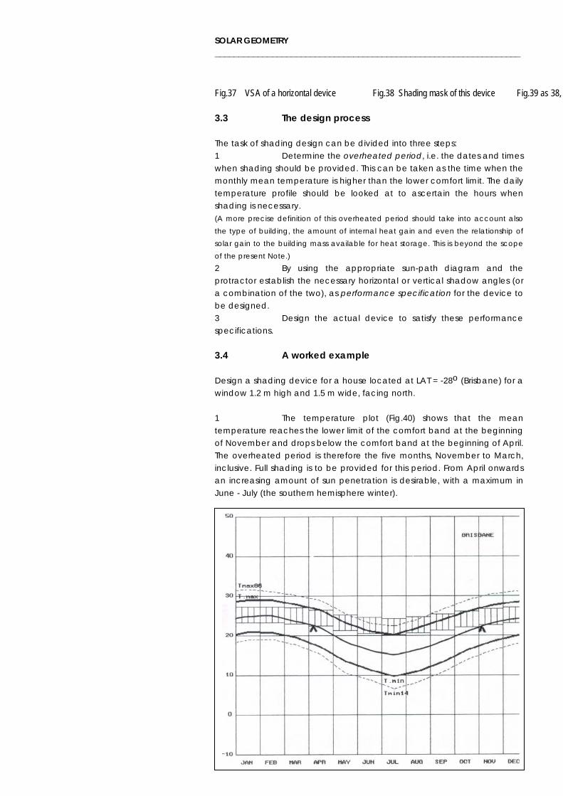
Fig.37 VSA of a horizontal device Fig.38 Shading mask of this device Fig.39 as 38, 3.3 The design process The task of shading design can be divided into three steps: 1 Determine the overheated period, i.e. the dates and times when shading should be provided. This can be taken as the time when the monthly mean temperature is higher than the lower comfort limit. The daily temperature profile should be looked at to ascertain the hours when shading is necessary. (A more precise definition of this overheated period should take into account also the type of building, the amount of internal heat gain and even the relationship of solar gain to the building mass available for heat storage. This is beyond the scope of the present Note.) 2 By using the appropriate sun-path diagram and the protractor establish the necessary horizontal or vertical shadow angles (or a combination of the two), as performance specification for the device to be designed. 3 Design the actual device to satisfy these performance specifications. 3.4 A worked example Design a shading device for a house located at LAT = -28o (Brisbane) for a window 1.2 m high and 1.5 m wide, facing north. 1 The temperature plot (Fig.40) shows that the mean temperature reaches the lower limit of the comfort band at the beginning of November and drops below the comfort band at the beginning of April. The overheated period is therefore the five months, November to March, inclusive. Full shading is to be provided for this period. From April onwards an increasing amount of sun penetration is desirable, with a maximum in June - July (the southern hemisphere winter).

SOLAR GEOMETRY ________________________________________________________________

18

Fig.40 Temperature plots and comfort band for Brisbane 2 The sun-path diagram (Fig.41) shows that the April 1 sun-path (between March 22 and April 15, nearer to the former) is quite different from the November 1 line (interpolated half-way between the October 15 and November 13 lines). This is a clear indication that the variation of temperatures lag behind the sun's movement: the maximum occurs late January, a month after the summer solstice and the minimum in late July, a month after the winter solstice. The following requirements can be read: April 1: VSA = 57o November 1: VSA = 77o For an exact solution a fixed device of 77o VSA could be provided, with a retractable extension down to 57o (Fig.42). The compromise of 67o would give cut-off dates as about October 3 and March 10, but overheating is less tolerable than a slight underheating, therefore the compromise should be biased in the direction of more shading: say 62o VSA. This would give cut-off at the equinox dates. N.b. as the window faces due north, the 62o VSA exactly matches the equinox sun-path, thus there is no need to use the protractor and VSAs coincide with the ALT circles along the centreline of the diagram (always coincide with the centreline of the protractor). Fig.41 Sun-path diagram for Brisbane Fig.42 Combined fixed and retractable device If the window were to face (say) 20o, then the protractor would have to be used, turned to the 20o direction. (Fig.43). This shows that a horizontal

SOLAR GEOMETRY ________________________________________________________________

19

device is impractical for early morning low angle sun. A vertical device, a baffle on the eastern side of the window should be used to assist. For cut-off at the equinox dates several combinations are possible, e.g. VSA 50o with an HSA of 40o VSA 40o with an HSA of 53o Fig.43 The protractor superimposed for ORI = 20o One may also argue that some early morning solar heat input, say up to about 9:00 h, does not have any adverse effects, in which case a horizontal device with a VSA of some 48o is satisfactory, without any side baffle. 3 Fig.44 shows a plan and section of this window. If the edge of the shading is level with the window head, then the projection must be x = 1.2 / tan50o = 1 m or x = 1.2 / tan40o = 1.43 m respectively. The east-side baffle should project y = 1.5 / tan40o = 1.78 or y = 1.5 / tan53o = 1.13 m Choosing the first alternative: the 1 m eaves projection, the 1.78 m vertical baffle is clearly impractical. Perhaps two fins (as shown) of 1.78 / 2 = 0.89 m would be acceptable.

Fig.44 Section and plan of the device designed and its shading mask

SOLAR GEOMETRY ________________________________________________________________

20

What is important is that the numerical results must be mitigated by intelligence, by qualitative judgements. 3.5 Overshadowing The concept of shading masks can be extended to evaluate the overshadowing effect of adjacent buildings or other obstructions. This technique is best illustrated by an example. Question: For what period is a point A of a proposed building overshadowed by the neighbouring existing building? Assume that the building is located at 42o latitude and it is facing 135o (S/E). Take a tracing of the shadow angle protractor and transfer onto it the angles subtended by the obstruction at point A, both on plan and section, as shown on Fig.45. This gives the shading mask of that building for the point considered. This can then be superimposed on the appropriate sun-path diagram (for 42o), with the correct orientation (135o) and the period of overshadowing can be read for the various dates. Fig.45 Plan, section ► and shading mask <- Fig.46 Shading mask laid over sun-path diagram ◄ In this instance just examine the three cardinal dates (Fig.46): - June 22: no overshadowing - Equinoxes: shade from sunrise to 11:00 h - Dec 22: shade from sunrise to about 10:40 h Fig.47 shows a more complex situation, where two existing buildings can cast a shadow over the point considered. To determine the outline for the altitude angles measured from sections use the shadow angle protractor so that its centreline is in the plane of section, e.g. direction X for section A-A and direction Y and Z for section B-B, as indicated in Fig.48, which explains the construction of the shading mask.

SOLAR GEOMETRY ________________________________________________________________

21

Fig.47 Overshadowing by two buildings Fig.48 The technique can also be used for a site survey: to plot all obstructing objects that may overshadow a selected point of the site. Fig.49 shows plan and sections of the site, with the existing buildings and Fig.50 explains the construction of the shading mask. Fig.49 Site survey: plan and four sections This shading mask can then be laid over the appropriate sun-path diagram and the period of overshadowing can be read, as indicated by Fig.51.

Fig.50 Construction of shading mask Fig.51 Shading mask laid over sun-paths

SOLAR GEOMETRY ________________________________________________________________

22

If a full-field camera, having a fish-eye lens were to be placed at point A, pointing vertically upwards, the photograph produced would be similar to this shading mask. A set of sun-path diagrams may be adapted for use as overlays to such photographs. 4 ALGORITHMS 4.1 Declination and equation of time Calendar dates are expressed as the number of day of the year (NDY), starting with January 1. Thus March 22 would be: NDY = 31 + 28 + 22 = 81 and December 31: NDY = 365. Declination is a sine function, which is zero at the equinoxes. To synchronize the sine curve with the calendar, the distance from the March equinox to the end of the year (284 days) is added to the NDY. As the year (365 days) corresponds to the full circle (360o), the ratio 360/365 = 0.986 must be applied as a multiplier, thus DEC = 23.45 * sin [0.986 * (284+NDY)] ... 1) A function more accurately fitted to the observed data is based on the leap-year correction: 360/366 = 0.9836. Using N = 0.9836 * NDY DEC = 0.33281 - 22.984 * cos N + 3.7872 * sin N - 0.3499 * cos(2*N) + 0.03205 * sin(2*N) - 0.1398 * cos(3*N) + 0.07187 * sin(3*N) ... 2) Both equations use degrees as the angular measure. For a computer program, where trigonometric functions use radians, eq.2 can be used with N = NDY * (2*Pi/366). The result will still be in degrees. A similar expression is available to obtain the equation of time values. This is the equation of the graph given in Fig.8. If, as above, N = 0.9836 * NDY then EQT = - 0.00037 - 0.43177 * cosN + 7.3764 * sinN + 3.165 * cos(2*N) 9.3893 * sin(2*N) - 0.07272 * cos(3*N) + 0.24498 * sin(3*N) ... 3) 4.2 Solar position angles The derivations of these expressions are given in Appendix 1. Altitude: ALT = arcsin(sinDEC * sinLAT + cosDEC * cosLAT * cos HRA) .. 4) where hour angle, HRA = 15 * (hour - 12) Azimuth: AZI = arccos[(cosLAT*sinDEC-cosDEC*sinLAT*cosHRA)/cosALT] ... 5) or

SOLAR GEOMETRY ________________________________________________________________

23

AZI = arcsin[(cosDEC * sinHRA) / cosALT] ... 6) results will be between 0 and 180o, i.e. for am only; for afternoon hours take AZI = 360 - AZI 4.3 Sunrise Sunrise hour-angle: SRH = arcos(-tanDEC * tanLAT) ... 7) Sunrise time: SRT = 12 - [arcos(-tanDEC * tanLAT)/15] ... 8) Azimuth at sunrise: SRA = arcos(cosLAT*sinDEC + tanLAT*tanDEC*sinLAT*cosDEC) ... 9) 4.4 Shadow angles Vertical: VSA = arctan(tanALT/cosHSA) . 10) Horizontal: HSA = AZI - ORI . 11) if 90o < abs|HSA| < 270o then sun is behind the facade, it is in shade if HSA > 270o then HSA = HSA - 360o if HSA <-270o then HSA = HSA + 360o 4.5 Angle of incidence Generally: INC = arcos(sinALT*cosTIL + cosALT*sinTIL*cosHSA) . 12) where TIL = tilt angle of receiving plane from horizontal For vertical planes, as TIL = 90, cosTIL = 0, sinTIL = 1 INC = arcos(cosALT * cosHSA) . 13) For a horizontal plane INC = ZEN = 90 - ALT . 14)

SOLAR GEOMETRY ________________________________________________________________

24

Summary of angles and terms used geographical

LAT geographical latitude (south negative) NDY day number (number of day of year) DEC solar declination (the angle between the earth-sun line, i.e. the ecliptic, and earth’s equator) ORI orientation (azimuth of the surface normal, or bearing) 0 to 360°from North, clockwise

solar

ALT altitude angle, from horizontal (0) to vertical (90°) AZI azimuth angle, 0 to 360°, clockwise ZEN zenith angle of the sun’s direction, from the vertical HSA horizontal shadow angle, from the surface normal, or azimuth difference, clockwise +ve, anticlockwise –ve VSA vertical shadow angle, within a plane perpendicular to a vertical surface, from horizontal to the line of the edge of a shading device INC angle of incidence on a surface, between the beam radiation (e.g. light) and the surface normal HRA solar hour angle, the sun’s direction from the solar noon, 15° per hour, -ve for the morning, +ve for afternoon SRA sunrise azimuth, the azimuth angle of the sun, unobstructed, at sunrise, measured in the horizontal plane SRT sunrise time, i.e. the time between sunrise and solar noon

SOLAR GEOMETRY _________________________________________________________________

25

5 SUN-PATH DIAGRAMS 5.1 Description Stereographic sun-path diagrams have been devised by Phillips in 1948. Petherbridge (1965) published a set of similar charts and an extended set of overlays (for solar heat gain calculations). Later, in an edited form, this was published by HMSO (Petherbridge, 1969). A series of such charts have been included in Koenigsberger et al (1973), where the use of these charts is also explained. The publications listed below also provide such explanations. Fig.52 shows the shadow angle protractor (introduced in Section 3.2, Fig.33) and Fig.53 is an example of a sun-path diagram for Lat. 36°, drawn manually using the method described in Appendix 2., This method is also included in the draft international standard ISO 6399-1. Fig.54 is the corresponding diagram produced by the program “ShadeDesign”. Fig.52 The shadow angle protractor (stereographic) This small computer program has been produced under Visual Basic, which can be downloaded separately. It will construct the sun-path diagram for any latitude and can be used for the design of shading devices. Diameter: Phillips (1948) used 4.5" (114 mm) diameter charts. Petherbridge used a diameter of 6" (153 mm) and the ISO 6399 recommends 150 mm. In Koenigsberger (1973) we used 150 mm charts, with dual lettering: to be used upside-down for southern latitudes. We now think that this is rather confusing. Here a diameter of 120 mm has been adopted to suit the limitations of some computers. Correspondingly the protractor is also of 120 mm diameter. Date lines: All charts show the solstice and the equinox sun-paths. ISO follows the UK practice of showing eight intermediate date lines (4 on each side) and does not show the altitude circles (a separate protractor must be used). Here the example of Phillips (1948) is followed: the altitude circles are shown and four intermediate date lines (2 on each side), but these are more evenly spaced. A total of 7 sun-path dates are shown in Table 1.

SOLAR GEOMETRY ________________________________________________________________

26

Fig.53 Sun-path diagram for latitude 36° – constructed manually Fig.54 Same as Fig.53, but produced by the program “ShadeDesign”

SOLAR GEOMETRY _________________________________________________________________

27

Note that the sun-path dates are marginally different: for the latter the declination was fixed and the date selected to match, see Table 1 Table 1 Dates of sun-paths and corresponding declinations 1) June 22 23.5° declination 2) May 12 Aug.1 18° 3) Apr. 14 Aug.28 9° 4) March 22 Sep 21 0 5) Feb.27 Oct.14 - 9 6) Jan.30 Nov.11 -18° 7) Dec.22 -23.5° Hour lines: In the D L I book(1975) the hour lines are half of the analemma (Fig.9), which allows for the ‘equation of time’ (eq.3 in Section 4.1) but necessitates two charts for each location. All other publications use simple arc-of-circle lines. ISO and its UK originals use such lines at half-hour intervals. We use only hourly lines. These are labelled using a 24-hour clock. Note that for the hour lines solar time is used, thus for the equinox dates the sun rises at 6:00 h exactly at the east-point and sets at 18:00 h, exactly at the west. Interpolation between dates (vertically) and hour lines (horizontally) is considered to be sufficiently accurate for sketch design purposes. There is a limit to accuracy achievable with such graphs used with a protractor. Even larger size (say 180 mm) diagrams will not give a significant improvement. 5.2 The program ShadeDesign When the program is called up and the START button is clicked, the circular chart-base is displayed, with the concentric altitude circles: 0° at the horizon circle and 90° at the centre point. (10 degree increments). The latitude is now to be input: northern +ve southern –ve. (Generally, after each input the ‘Tab’ key is to be pressed.) Then there is a choice: to show all 7 sun-paths, or (to have a cleaner picture) show only the 3 main lines. The pairs of dates for each line (as above) are shown in a table next to the chart base (same as Table 1 above). Alternatively, one can opt for the “path for given date” , in which case the date must be input (month number, day number), then a click on “draw” will produce a single sun-path line for that date. If the orientation of the façade considered is input (0 to 360°, clockwise), a click on “protractor” will position the shadow angle protractor over the chart (in green outline). If the ‘overheated period’ is identified on the sun-path chart, the purpose is to find a VSA or HSA (or a combination) shading mask that would cover or almost cover this overheated period. A VSA or one or two HSA values can be input (any one or two or all three) and a click on “show” will display the corresponding shading mask. Any number of such angles can be displayed by just overtyping the previous angles in the input windows. If the diagram gets messy, click on “other shading” and all masks will be erased.

SOLAR GEOMETRY ________________________________________________________________

28

The button “another” will clear the screen and the process can be re-started for the same latitude. The latitude can be overtyped if another location is to be considered. The advantage of these charts is that they show a pattern of variations in time, thus they are eminently useful at the sketch design stage. If the implied tolerances (inaccuracy) is not accepted, it is suggested that, having decided on a design by using these charts, the critical angles should be calculated by the equations given in Section 4. 5.3 A worked example Fig.55 is a screen printout of ShadeDesign. The latitude was input as ‘-27.5’ and the “all 7 sun-paths” option was chosen. The “orientation” box got the input ‘30’ and the “protractor” key pressed, to get the shadow angle protractor, with its centreline pointing at 30° (green outline). Assume that the half-year above the equinox sun-path is the ‘overheated period’, when the sun should be excluded. The afternoon times, below and to the left of the protractor’s base line are of no interest, as the sun is behind the building. Try a VSA of 50° and click on “show”. The arcual line of the protractor appears, which at its centreline coincides with the 50° altitude circle (count up five circles from the horizon. This shows that on equinox dates, from just before 10 h the point considered will be shaded, but in the summer months the morning sun will penetrate: on December 22 only up to 6:00, on Nov.11/ Jan 30 up to just after 7:00 and on Aug.28 / Apr.14 up to about 8:50. Fig.55 Working with the ShadeDesign program

SOLAR GEOMETRY _________________________________________________________________

29

To exclude this morning sun, a vertical device to the right-hand side of the window would be best, characterised by a positive HSA: try +40°. When the “show” button is clicked the radial line appears, intersecting the perimeter 40° clockwise from the centreline. This crosses the VSA arc at about 9:00 h, showing that the shading is almost complete, except a little time around 9 h at the equinox. As the definition of the overheated period is only an informed guess, we may decide that this solution: +40°HSA plus a VSA of 50° is acceptable. Clicking on the “print form” button at this point produced the chart of Fig.55. A more pedantic way of determining the shading (overheated) period is shown by an example of Phoenix (AZ), Lat = 35.5° months: coldest hottest Jan. Jul. outdoor mean T ⎯T 11°C 32.5°C neutrality T Tn 21 27.7 limits 18.5 30.2 where Tn = 17.6 + 0.31 x⎯T limits are taken as Tn ±2.5 K Winter: at 18.5°C solar heat input is definitely desirable, but as the neutrality is 21°C, some solar input at this temperature may be acceptable. Summer: above the neutrality (27.7°C) solar heat input is undesirable, as there will be some incidental solar and internal gains, so the upper limit of 30.2°C may be reached anyway. The annual temperature changes can be shown on a month x hour chart by isotherm lines. Here the three lines: 18.5, 21 and 27.7°C are plotted. (Fig.A) These isotherms can be transferred to the sun-path diagram, as that is actually also a month x hour (curved lines) graphs, and the curvature of lines can be ignored (Fig. B). Two such diagrams are needed (as each sun-path line represents two dates):

Fig. A Annual temperature isotherms

Fig. B Isotherms transferred to the sun-path diagram: the first one for June to December and the second for December to June. Below the bottom curve (18.5°C) solar input is desirable. It is acceptable to the middle one (21°C). Shading is a must above the top one (27.7°C).

SOLAR GEOMETRY ________________________________________________________________

30

References D L I, (Department of Labor and Immigration) (1975): Control of sunlight

penetration. Industrial Data Sheets A2. AGPS (Australian Government Publishing Service), Canberra

Henry Hope & Sons Ltd. (1964): Solar charts and shadow angle protractor.

Catalogue No.374. Birmingham International Standards Organisation (1995): Draft International Standard

6399-1: Climatic data for building design - Solar radiation - Sunpath diagrams.

Koenigsberger, O. H. et al. (1973): Manual of tropical housing and building,

Pt.1: Climatic design. Longman, London Petherbrdige, P (1965): Sunpath diagrams and overlays for solar heat gain

calculations. Current Paper (Research series) 39, Building Research Station, Garston

Petherbridge, P (1969): Sunpath diagrams and overlays for solar heat gain

calculations. HMSO (Her Majesty's Stationery Office), London Phillips, R. O. (1948): Sunshine and shade in Australasia. Technical Study

No.23, Commonwealth Experimental Building Station, Sydney. Now available as Bulletin No. 8 (5th ed.) of the National Building Technology Centre, 1987

Szokolay, S. V. (1980): Environmental science handbook for architects and

builders. Longman/Construction Press, London

SOLAR GEOMETRY _________________________________________________________________

31

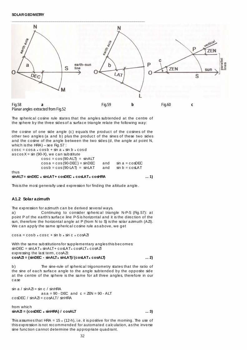
APPENDIX 1 Derivations of solar angle equations A1.1 Solar altitude Fig.56 shows the earth and indicates the relevant angular relationships. - Point P on the earth's surface is the location considered. - The angle between the radius of P and the plane of the equator is the latitude (LAT). The extension of this radius outwards from P is the vertical, pointing at the zenith. - The line from the centre of earth (O) to the centre of the sun is referred to as the earth-sun line (which lies within the ecliptic plane – see Fig.2) and it intersects the earth's surface at point S. At this point S the sun appears to be at the zenith. The longitude of point S is the solar noon longitude. - The angle between the earth-sun line and the plane of the equator is the declination (DEC). - The angle between the solar noon longitude (i.e. the plane of quadrant N-O-M) and the longitude of P (i.e. the plane of quadrant N-O-L) is the hour angle (HRA). Fig.56 Spherical trigonometry: the earth-sphere and various angles for analytical treatment Consider the spherical triangle N-P-S (Fig.57, extracted from Fig.56). The planar angles subtended at the centre of the earth (O) are, as shown in Figs.57-59, (also extracted from Fig.56): - the earth's centre and the radius of point S (the earth-sun line, Fig.58): a = 90 - DEC - between the earth's axis and the radius of point P (Fig.59): b = 90 - LAT - between the radii of points S and P (the earth-sun line and the local vertical, Fig.60): c = ZEN = 90 - ALT The angle at the north pole (N) between the local longitude and the solar noon longitude: d = HRA

Fig.57 Spherical triangle N-P-S extracted

SOLAR GEOMETRY ________________________________________________________________

32

Fig.58 a Fig.59 b Fig.60 c Planar angles extracted from Fig.52 The spherical cosine rule states that the angles subtended at the centre of the sphere by the three sides of a surface triangle relate the following way: the cosine of one side angle (c) equals the product of the cosines of the other two angles (a and b) plus the product of the sines of these two sides and the cosine of the angle between the two sides (d, the angle at point N, which is the HRA) – see Fig.57 : cos c = cos a * cos b + sin a * sin b * cos d as cos X = sin (90-X), we can substitute cos c = cos (90-ALT) = sinALT cos a = cos (90-DEC) = sinDEC and sin a = cosDEC cos b = cos (90-LAT) = sinLAT and sin b = cosLAT thus sinALT = sinDEC * sinLAT + cosDEC * cosLAT * cosHRA ... 1) This is the most generally used expression for finding the altitude angle. A1.2 Solar azimuth The expression for azimuth can be derived several ways. a) Continuing to consider spherical triangle N-P-S (Fig.57): at point P of the earth's surface line P-S is horizontal and it is the direction of the sun, therefore the horizontal angle at P (from N to S) is the solar azimuth (AZI). We can apply the same spherical cosine rule as above, we get cos a = cos b * cos c + sin b * sin c * cosAZI With the same substitutions for supplementary angles this becomes: sinDEC = sinLAT * sinALT + cosLAT * cosALT * cosAZI expressing the last term, cosAZI: cosAZI = (sinDEC - sinALT * sinLAT)/(cosLAT * cosALT) ... 2) b) The sine-rule of spherical trigonometry states that the ratio of the sine of each surface angle to the angle subtended by the opposite side at the centre of the sphere is the same for all three angles, therefore in our case sin a / sinAZI = sin c / sinHRA as a = 90 - DEC and c = ZEN = 90 - ALT cosDEC / sinAZI = cosALT / sinHRA from which sinAZI = (cosDEC * sinHRA) / cosALT ... 3) This assumes that HRA = 15 * (12-h), i.e. it is positive for the morning. The use of this expression is not recommended for automated calculation, as the inverse sine function cannot determine the appropriate quadrant.

SOLAR GEOMETRY _________________________________________________________________

33

A1.3 Derivations by planar geometry A different set of derivations is possible by using planar geometry only. Fig.61 is a sectional view of the sky hemisphere at the location considered, bounded by the local noon meridian circle, looking towards the east, so that north is on the left and south on the right (southern hemisphere), with the zenith on the top. The diagonal line going through the centre (line EO) is the ‘side elevation’ of the equinox sun-path. This is tilted from the vertical by an angle equal to the latitude (LAT), in this example -41o. By convention southern latitudes are negative. The December and June sun-paths are located by drawing two radii from point O, at -23.45o up (D) and +23.45o down (J) from the equinox sun-path and where these meet the meridian, draw parallel lines with the equinox sun-path. (These are the ‘side elevations’ of the sun-paths at the solstices.) A small semicircle can be drawn at the tangent to the equinox path, with its centre at point E. If the sky hemisphere radius is taken as 1, then from the triangle JOE' the radius of this small semicircle will be JE' (= EJ' = ED') = sin 23.45 = 0.39795. The sun-path line for any intermediate date can be located with the aid of this small semicircle, by drawing a radius to the slope of dn*(180/182.5), where dn is the day number counted from December 22 in both directions (the bracketed term is the same as 360/365). Fig.61 Sectional view of the local sky hemisphere Fig.62 The sun's position defined on the sky hemisphere Fig.62 is the same diagram, but the sun is located on it at point S. The corresponding sun-path line can be drawn in and extended to point B. Drawing a radius to this point and measuring its slope (in this example 60o) the date can be determined from the above relationship:

SOLAR GEOMETRY ________________________________________________________________

34

dn*(180/182.5) = 60 from which dn = 60 * (182.5/180) = 61 thus the date is 61 days either before or after December 22 (Feb. or Oct. 22) A radius of the large circle drawn to the sun-path's intersection point (A) will subtend the declination angle (DEC) at the centre. In the small semicircle from triangle BEA' the base line will be, in this example EA' = 0.39795 * cos 60o = 0.2 but as it is the December half-year, it will be -0.2. In the larger circle, from triangle AOE" the angle at O is the declination. As OA = 1 and AE" = EA' sinDEC = EA' in this example DEC = arcsin(-0.2) = -11.5o The location of point S, within the meridian plane along the above sun-path line can be defined by determining the distance ZH. This ZH = ZG + GH and the two components can be determined separately. From the triangle AOG the angle at O is LAT - DEC. As OA = 1 and OG = cos (LAT-DEC). In our example: OG = cos[-41-(-11.5)] = cos(-29.5) = 0.87 The trigonometrical identity can be applied: cos(LAT-DEC) = cosLAT*cosDEC + sinLAT*sinDEC As ZG = 1 - OG here ZG = 1 - 0.87 = 0.13 ZG = 1 - (cosLAT*cosDEC + sinLAT*sinDEC) ... 4) From the small triangle ACS the angle at S is the same as LAT, the distance CS is the same as GH, thus GH = AS * cosLAT ... 5) The distance AS is proportionate to the time from noon and will be determined below; first: from triangle AOF the angle at A is the same as DEC and as OA = 1 AF = cos DEC in this example cos(-11.5) = 0.98 In Fig.62 the line OE is the 'side elevation' of the equinox sun-path, with point S projected onto this as S". Fig.63 is a full perpendicular view of this sun-path (the OE radius is the same), where the hour angle is HRA = 15 * (h - 12) in our example for 8.30 am: HRA = 15*(8.5-12) = -52.5o As OS' = 1, the distance OS" = cosHRA here cos(-52.5) = 0.61 and ES" = 1 - cosHRA here 1 - 0.61 = 0.39 Switching back to Fig.58: A'S corresponds to ES" and AS will be slightly less, by the proportion AF/EO. But EO = 1 and AF = cosDEC, thus AS = cosDEC * (1-cosHRA) ... 6) in the example cos(-11.5) * (1-0.61) = 0.382 Fig63 View of the sun-path examined (EO = A'F in Fig.62)

SOLAR GEOMETRY _________________________________________________________________

35

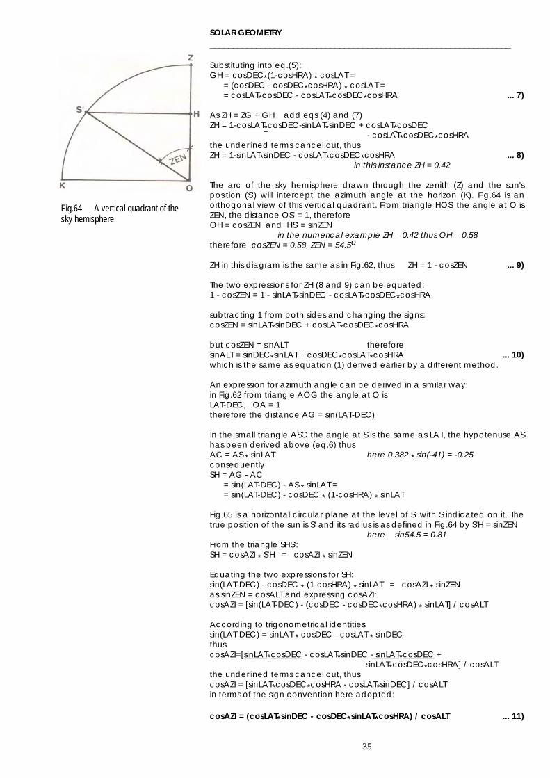
Substituting into eq.(5): GH = cosDEC*(1-cosHRA) * cosLAT = = (cosDEC - cosDEC*cosHRA) * cosLAT = = cosLAT*cosDEC - cosLAT*cosDEC*cosHRA ... 7) As ZH = ZG + GH add eqs (4) and (7) ZH = 1-cosLAT*cosDEC-sinLAT*sinDEC + cosLAT*cosDEC - cosLAT*cosDEC*cosHRA the underlined terms cancel out, thus ZH = 1-sinLAT*sinDEC - cosLAT*cosDEC*cosHRA ... 8) in this instance ZH = 0.42 The arc of the sky hemisphere drawn through the zenith (Z) and the sun's position (S') will intercept the azimuth angle at the horizon (K). Fig.64 is an orthogonal view of this vertical quadrant. From triangle HOS' the angle at O is ZEN, the distance OS' = 1, therefore OH = cosZEN and HS' = sinZEN in the numerical example ZH = 0.42 thus OH = 0.58 therefore cosZEN = 0.58, ZEN = 54.5o ZH in this diagram is the same as in Fig.62, thus ZH = 1 - cosZEN ... 9) The two expressions for ZH (8 and 9) can be equated: 1 - cosZEN = 1 - sinLAT*sinDEC - cosLAT*cosDEC*cosHRA subtracting 1 from both sides and changing the signs: cosZEN = sinLAT*sinDEC + cosLAT*cosDEC*cosHRA but cosZEN = sinALT therefore sinALT = sinDEC*sinLAT + cosDEC*cosLAT*cosHRA ... 10) which is the same as equation (1) derived earlier by a different method. An expression for azimuth angle can be derived in a similar way: in Fig.62 from triangle AOG the angle at O is LAT-DEC, OA = 1 therefore the distance AG = sin(LAT-DEC) In the small triangle ASC the angle at S is the same as LAT, the hypotenuse AS has been derived above (eq.6) thus AC = AS * sinLAT here 0.382 * sin(-41) = -0.25 consequently SH = AG - AC = sin(LAT-DEC) - AS * sinLAT = = sin(LAT-DEC) - cosDEC * (1-cosHRA) * sinLAT Fig.65 is a horizontal circular plane at the level of S, with S indicated on it. The true position of the sun is S' and its radius is as defined in Fig.64 by S'H = sinZEN here sin54.5 = 0.81 From the triangle SHS': SH = cosAZI * S'H = cosAZI * sinZEN Equating the two expressions for SH: sin(LAT-DEC) - cosDEC * (1-cosHRA) * sinLAT = cosAZI * sinZEN as sinZEN = cosALT and expressing cosAZI: cosAZI = [sin(LAT-DEC) - (cosDEC - cosDEC*cosHRA) * sinLAT] / cosALT According to trigonometrical identities sin(LAT-DEC) = sinLAT * cosDEC - cosLAT * sinDEC thus cosAZI=[sinLAT*cosDEC - cosLAT*sinDEC - sinLAT*cosDEC + sinLAT*cosDEC*cosHRA] / cosALT the underlined terms cancel out, thus cosAZI = [sinLAT*cosDEC*cosHRA - cosLAT*sinDEC] / cosALT in terms of the sign convention here adopted: cosAZI = (cosLAT*sinDEC - cosDEC*sinLAT*cosHRA) / cosALT ... 11)

Fig.64 A vertical quadrant of the sky hemisphere

SOLAR GEOMETRY ________________________________________________________________

36

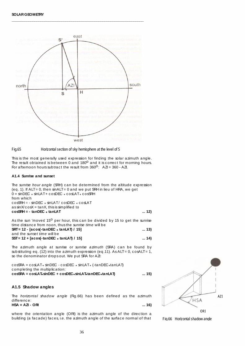
Fig.65 Horizontal section of sky hemisphere at the level of S This is the most generally used expression for finding the solar azimuth angle. The result obtained is between 0 and 180o and it is correct for morning hours. For afternoon hours subtract the result from 360o: AZI = 360 - AZI. A1.4 Sunrise and sunset The sunrise hour angle (SRH) can be determined from the altitude expression (eq. 1). If ALT = 0, then sinALT = 0 and we put SRH in lieu of HRA, we get 0 = sinDEC * sinLAT + cosDEC * cosLAT * cosSRH from which cosSRH = - sinDEC * sinLAT / cosDEC * cosLAT as sinX/cosX = tanX, this is simplified to cosSRH = - tanDEC * tanLAT ... 12) As the sun 'moves' 15o per hour, this can be divided by 15 to get the sunrise time distance from noon, thus the sunrise time will be SRT = 12 - [acos(-tanDEC * tanLAT) / 15] ... 13) and the sunset time will be SST = 12 + [acos(-tanDEC * tanLAT) / 15] ... 14) The azimuth angle at sunrise or sunrise azimuth (SRA) can be found by substituting eq. (12) into the azimuth expression (eq.11). As ALT = 0, cosALT = 1, so the denominator drops out. We put SRA for AZI: cosSRA = cosLAT * sinDEC - cosDEC * sinLAT * (-tanDEC*tanLAT) completing the multiplication: cosSRA = cosLAT*sinDEC + cosDEC*sinLAT*tanDEC*tanLAT) ... 15) A1.5 Shadow angles The horizontal shadow angle (Fig.66) has been defined as the azimuth difference: HSA = AZI - ORI ... 16) where the orientation angle (ORI) is the azimuth angle of the direction a building (a facade) faces, i.e. the azimuth angle of the surface normal of that

AZI

ORI

Fig.66 Horizontal shadow angle

SOLAR GEOMETRY _________________________________________________________________

37

facade. This means that when AZI < ORI, the sun is to the left, or anticlockwise of the orientation, the HSA is negative. When AZI > ORI, HSA is positive, the sun is to the right, or clockwise. The result is meaningful only up to |90o|. A larger value indicates that the sun is behind the facade considered and will not reach that facade. For automated calculation a check-routine must be built in: if 90o<|HSA|<270o then the facade is in shade if HSA > 270o then take it as HSA = HSA - 360o if HSA <-270o then take it as HSA = HSA + 360o The vertical shadow angle has been defined by Figs.31-32. It can be seen that when HSA = 0, then VSA = ALT. As the HSA is increasing, the VSA is also increasing. This increase is inversely proportionate to the cosine of HSA. tan VSA = tan ALT / cosHSA A1.6 Angle of incidence The angle of incidence (INC) of solar radiation on a given plane surface is measured between the direction of the beam and the surface normal. Thus for a horizontal surface the angle of incidence is the same as the zenith angle (Fig.67): INC = ZEN = 90 -ALT For a vertical surface the cosine rule applies (Fig. 68): cosINC = cosALT * cosHSA For the general case, ie. a tilted surface of any orientation (Fig.69), if the angle of tilt from the horizontal is TIL, a correction must be made for that tilt: cosINC = sinALT * cosTIL + cosALT * sinTIL * cosHSA ... 18) The previous two cases are special instances of this general expression. For a vertical surface TIL = 90o, cosTIL = 0, thus the first term drops out and sinTIL = 1, thus it can be omitted from the second term. For a horizontal surface, as TIL = 0, sinTIL = 0, thus the second term drops out; cosTIL = 1, thus we are left with cosINC = sinALT, which is the same as cosINC = cosZEN, thus INC = ZEN.

Fig.68 Angle of incidence on vertical Fig.69 Angle of incidence on a tilted surface

Fig.67 Angle of incidence on horizontal

SOLAR GEOMETRY ________________________________________________________________

38

References for the derivations Addleson, Lyall (1973): Sunlight geometry. Notes: Building Environment and

Services. Brunel University. Kittler, Richard (1981): A universal calculation method for simple

predetermination of natural radiation on building surfaces and solar collectors. Building and Environment, 16(3):177-182

Penrod, E. B. (1964): Solar load analysis by use of orthographic projections and spherical trigonometry. Solar Energy 8(4): 127-133

Robinson, N (1966): Solar radiation. Elsevier, 1966. (esp. chapter 2: The astronomical and geographical factors affecting the amount of solar radiation reaching the earth)

APPENDIX 2 Construction of stereographic sunpath diagrams 1 Draw a circle of selected radius (r). In this work r = 60 mm is used, several

publications use r = 75 mm (for a 150 mm diameter). Draw a horizontal and a vertical diameter to indicate the four cardinal compass points. Extend the vertical in the polar direction to give the locus for the centres of all sun-path arcs.

2 For each sun-path arc (for each selected date) calculate its radius (rs)

and the distance of its centre from the centre of the circle (ds): rs = r * cosDEC/(sinALT + sinDEC) ds = r * cosLAT /(sinLAT + sinDEC) where LAT = geographical latitude DEC = solar declination angle for March 22 and Sept.21 DEC = 0o June 22 DEC = 23.45o December 22 DEC = -23.45o For intermediate dates see the discussion and tabulation on p.24. 3 For the construction of the hour lines calculate the distance of the locus

of centres from the centre of the circle (dt) and draw this locus parallel to the east-west axis.

dt = r * tanLAT 4 For each hour calculate the horizontal displacement from the vertical

centreline (dh) and the radius of the hour-arc (rh): dh = r /(cosLAT * tanHRA) rh = r /(cosLAT * sinHRA) Fig.70 Construction of curves where HRA = hour angle from noon, 15o for each hour e.g.for 8:00 h: HRA = 15 * ( 8-12) = -60o

or for 16:00 h: HRA = 15 * (16-12) = 60o

SOLAR GEOMETRY _________________________________________________________________

39

5 Draw the arcs for the afternoon hours from a centre on the right-hand

side and for the morning hours from the left-hand side. A useful check is that the 6:00 and 18:00 h lines should meet the equinox sun-path exactly at the east and west points of the circle respectively.

6 Mark the azimuth angles on the perimeter at any desired increments in a

clockwise direction, from 0o to 360o (north) and construct a set of concentric circles to indicate the altitude angle scale.

For any altitude (ALT) the radius (ra) of the circle will be ra = r * cosALT /(1+sinALT) 7 For a shadow angle protractor draw a semi-circle to the same radius as

the chart. Extend the vertical axis downwards to give the locus for the centres of all VSA (vertical shadow angle) arcs. For each chosen increment of VSA find the displacement of the centre (dv) and the radius of the arc (rv):

dv = r * tanVSA rv = r / cosVSA 8 Mark the HSA (horizontal shadow angle) scale along the perimeter: the centreline is zero, then to 90o to the right (clockwise) and to -90o to the

left (anticlockwise). 9 Two useful checks: a) all the VSA arcs should meet at the corner of the semicircle and the

base line b) along the centreline of the protractor the VSA arcs should coincide

with the corresponding altitude circles of the sun-path diagram. It is relatively easy to write a computer program on the basis of the above algorithm. This algorithm is also used in the program ShadeDesign. My view is that these sun-path diagrams provide an excellent tool for manual work, which is assisted by this program. Much more sophisticated tools are also available for the design of shading devices and for the dynamic examination of their performance, possibly coupled with 3D CAAD images,.

Fig.71 Construction of protractor

SOLAR GEOMETRY ________________________________________________________________

40

APPENDIX 3 Some further applications: A3.1 Sun penetration The system of sun-path diagrams and protractor can be used to determine sun-penetration through an opening at a given time or a sequence of time points. The method is illustrated by an example: A 1 m square window, with a sill height of 0.9 m is facing 165o (S/SE). The location is LAT = 40o (say: southern Italy). Determine the sun penetration on February 26, at 10, 12 and 14 h. Take the 40o sun-path diagram and mark the three time points on the Feb.26 sun-path line (Fig.70). For HSA values use the perimeter scale and for the VSA values interpolate between the arcual lines. The readings at the three points can be tabulated as follows: h HSA VSA 10 -22 34 12 15 40 14 51 45__ Fig.72 Sunpath diagram for LAT = 40o with protractor overlaid facing 165 o Fig.73 Construction of sunlit patch Draw a plan and section of the window. Plot the HSAs on the plan: draw two parallel lines for each time-point, tangential to the window jambs (Fig71). These will determine the direction of sun penetration. The VSA is actually the projection of the solar altitude angle onto a vertical plane normal to the window considered, which is the plane of our 'section'. Therefore plot the VSAs on this section and draw two parallel lines for each time-point, touching the inside edge of the window sill and the outside edge of the head. These will mark on the floor the depth of sun penetration. Project these points back on the plan, defining the edges of the rhomboid-shaped sun-patch, parallel with the window plane.

SOLAR GEOMETRY _________________________________________________________________

41

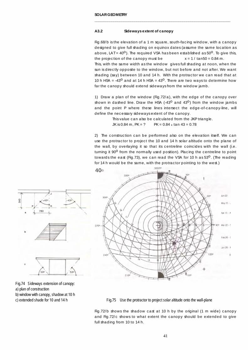
A3.2 Sideways extent of canopy Fig.68/b is the elevation of a 1 m square, south-facing window, with a canopy designed to give full shading on equinox dates (assume the same location as above, LAT = 40o). The required VSA has been established as 50o. To give this, the projection of the canopy must be x = 1 / tan50 = 0.84 m. This, with the same width as the window gives full shading at noon, when the sun is directly opposite to the window, but not before and not after. We want shading (say) between 10 and 14 h. With the protractor we can read that at 10 h HSA = -43o and at 14 h HSA = 43o. There are two ways to determine how far the canopy should extend sideways from the window jamb. 1) Draw a plan of the window (Fig.72/a), with the edge of the canopy over shown in dashed line. Draw the HSA (-43o and 43o) from the window jambs and the point P where these lines intersect the edge-of-canopy-line, will define the necessary sideways extent of the canopy.

This value can also be calculated from the JKP triangle. JK is 0.84 m, PK = ? PK = 0.84 * tan 43 = 0.78

2) The construction can be performed also on the elevation itself. We can use the protractor to project the 10 and 14 h solar altitude onto the plane of the wall, by overlaying it so that its centreline coincides with the wall (i.e. turning it 90o from the normally used position). Placing the centreline to point towards the east (Fig.73), we can read the VSA for 10 h as 53o. (The reading for 14 h would be the same, with the protractor pointing to the west.)

Fig.74 Sideways extension of canopy: a) plan of construction b) window with canopy, shadow at 10 h c) extended shade for 10 and 14 h Fig.75 Use the protractor to project solar altitude onto the wall-plane

Fig.72/b shows the shadow cast at 10 h by the original (1 m wide) canopy and Fig.72/c shows to what extent the canopy should be extended to give full shading from 10 to 14 h.

SOLAR GEOMETRY ________________________________________________________________

42

APPENDIX 4 Model studies Several devices have been developed to simulate the solar geometry and allow the study of shading using building models. The value of these devices as design tools is rather doubtful, but they are certainly useful as learning tools, or for checking the performance of devices designed, or for the purposes of demonstration, possibly by photographs of the model with shadows cast on different dates and times. Such photos can be quite useful in some controversial building permit applications (or opposition thereto), for presentation to clients or even in some court cases. All these devices employ a light source to simulate the sun. A point source will give a divergent beam at the model, resulting in shadows of parallel lines becoming divergent. To reduce this effect the lamp-to-model distance can be increased or a light source of extended diameter can be used. In order to represent the sun - building relationship the device must allow for three geometrical adjustments: - geographical latitude - date of the year (calendar) - time of the day. The oldest such device is the heliodon (Fig.74). With this the model must be fixed to the table, which tilts to simulate the geographical latitude. The table will be horizontal for the poles and vertical for the equator. The time of day is simulated by the rotation of this table. The lamp representing the sun is mounted at a fixed distance on a slider of a vertical rail, so that it can slide up and down, providing for the calendar adjustment. The mid-point, level with the centre of the table, is the equinox, the topmost position the summer solstice and the lowest position is mid-winter. Eg. if the distance from the centre of the table to the lamp is 3 m, the slider must be able to move 3 x tan 23.45o = 1.3 m up and down from the equinox position. Fig.76 The heliodon

SOLAR GEOMETRY _________________________________________________________________

43

The solarscope (Fig.75) has a table, which remains horizontal. The "sun", represented by a circular mirror, is mounted at the end of a long arm, with a spotlight at the lower end of this arm aimed at the mirror. (This effectively doubles the lamp-to-model distance.) This arm swings around a horizontal axis to represent the hour of day and tilts forward or up to give the calendar adjustment. The table can be lowered, which will lift the fulcrum of the arm (or raised, lowering this fulcrum) - providing the latitude adjustment. The best solarscope (at least for educational purposes) is shown in Fig.72. The sun is a lamp placed at the focal point of a parabolic mirror of 600 - 750 mm diameter (e.g. a searchlight mirror), to give a broad parallel beam of light. This is mounted on a motorised carriage travelling on a semicircular rail (or rather 3/4 of a circle) to indicate the time of day. This rail itself is mounted on sliders moving along a cross-bar at both ends, to give the calendar adjustment. The two cross-bars themselves tilt to give the adjustment for geographical latitude.

Fig.77 Solarscope of the CEBS, Sydney (Commonwealth Experimental Building Station)

Fig.78 The most realistic solarscope The advantage of this solarscope is that the model table is fixed and that the rail indicates the sun's path for the particular date, so it facilitates easy visualisation of the real situation. A simplified version of this solarscope consists of three semicircular arcs (e.g. of metal tubes) fixed to two tilting cross-rails (Fig.77). The tilting gives the latitude adjustment and the three rails represent the equinox and the two solstice sun-paths. Small lamps are fixed to these arcs at 15o intervals, which are individually switchable ( 3 times 13 lamps), to represent the sun for that date and hour. The small light sources present the problem of divergent shadows.

SOLAR GEOMETRY ________________________________________________________________

44

Fig.79 A simplified solarscope Three sun-path arcs with 39 lamps. Tilt: latitude adjustment. If the device is to be used only for one given location, then the tilting rails can be avoided and we can have just the three arcs fixed to a table. The simplest of all methods is the use of a small sun-dial (e.g. the matchbox-type, shown in Fig.78). This can be attached to the building model, with the correct orientation, which can then be turned and tilted - under open-air sunlight - until the shadow of the gnomon shows the required date and hour. Not very accurate, but it allows the taking of good photos and it certainly avoids the problem of divergent light-beam. Fig.80 A matchbox-type sun-dial (for northern hemisphere) Fold and paste inside a matchbox-drawer. Fix a 14 mm high stick as a gnomon at the + point. Fix to model with matching the north-points.

SOLAR GEOMETRY _________________________________________________________________

45

Index analemma 7, 27 algorithm 22 altitude 6, 8, 10, 22, 23, 31, 32, 37 altitude circles 9 angle of incidence 23, 37 aphelion 5, 7 azimuth 6, 10, 22, 32, 35 Cancer, tropic of 6 Capricorn, tropic of 6 cylindrical projection 11 declination 5, 22, 27, 31, 33, 38 ecliptic 5, 31 equation of time 7, 22, 27 equator 5, 6, 31 equidistant chart 9, 12, 13 equinox 5, 8, 20, 42 full-field camera 21 gnomonic projection 13, 14 heliodon 42 hour angle 6, 31, 34, 38 latitude 5, 6, 8, 31, 33, 36, 38 local (mean~) time 7 meridian 6, 7 nadir 9, 10 noon 6, 7 orbit 5 orthographic projection 9 orientation 15, 23, 28, 36 overheated period 17, 27, 29 overshadowing 20, 21 perihelion 5, 7 planar geometry 33, 34 references 29, 38 ShadeDesign program 3, 27 shading devices 15, 16, 18, 19, 41 shading mask 16, 19, 20, 21, 28 shadow angle 15, 23, 36, 41 -- horizontal 15, 16, 19, 23, 25, 27, 37, 40 -- protractor 16, 18, 19, 25, 28, 39, 40, 41 -- vertical 15, 16, 18, 23, 25, 27, 37, 40 site survey 21 solarscope 43, 44 solar time 7 solstice 5, 24, 27, 42, 43 spherical geometry 31, 32 -- triangle 31 -- trigonometry 31 stereographic projection 9, 10, 25 sun-dial 13, 44 sun-path diagram 9, 10, 18, 19, 21, 25-28, 38, 41 -- construction of 38 sun-path lines 8, 9, 12, 13 sun penetration 40 sunrise 23, 36 sunset 36 tropics 6 vertical sun-path diagrams 11-13 Waldram projection 11 zenith angle 6, 8, 31,33, 35, 37