Playing Tic-tac-toe with the NAO humanoid robot

Renzo Poddighe

July 1, 2013

Abstract

This paper describes the challenges that haveto be tackled when playing a game of tic-tac-toe with the NAO humanoid robot. The mostimportant aspects of tic-tac-toe for a robot aresolving the Inverse Kinematics problem, andanalyzing the game board using image process-ing. It succeeded in drawing om the board us-ing the FABRIK algorithm for moving the arm,and Hough line and circle transform for recog-nizing the board and the symbols.

1 Introduction

This paper covers the aspects involved in enabling aNAO humanoid robot to physically play a game of Tic-tac-toe against a human player. The main focus is oncoordinating the NAO’s arm movements, which concernssolving the Inverse Kinematics problem, but also recog-nizing the board using image processing.

Moving the arm may seem like a straightforward task,but is in fact quite difficult to accomplish for a robot. Ahuman’s capability of interpreting its environment moreheuristically outperforms the robot’s generally moremathematical approach in this case. The mathematicaldescription of the Inverse Kinematics problem is a non-linear system of equations with possibly multiple solu-tions. Traditional methods are computationally expen-sive, because they rely on constructing and operating onlarge and complex matrices. Furthermore, the NAO doesnot possess that much processing power. An computa-tionally cheap approach that comes up with solutionsmore efficiently is therefore the preferred approach inthis case.

Recognizing the board is another example of taskwhich is obvious for a human because of the brain’s abil-ity to interpret and match patterns, but a more difficulttask for a robot. Fortunately, image processing softwarecontaining algorithms that are sufficient for this rela-tively simple task is freely available. Playing Tic-tac-toeis a well-known problem, and is easily solvable by a com-puter. A basic minimax search algorithm is sufficient inthis research.

1.1 Research questions

The research questions this paper focuses on are:

1. How is the drawing of a circle and a cross in thecorrect square of the game board coordinated?

2. Is the NAO capable of recognizing the figures onthe board and interpreting them in the context oftic-tac-toe?

1.2 Structure

This section contains an overview of all the tasks thatare tackled in this paper, as well as the structure of thispaper and an overview of the terms used in this paper. InSection 2, information about the hardware and softwareis listed. Section 3 describes the preliminaries and identi-fies relevant research challenges. Section 4 describes theapproaches used to enable the NAO to play tic-tac-toe.The implementation of these approaches can be foundin Section 5. Finally, the conclusion about the researchand some suggestions for future research can be foundin Section 6.

1.3 Terminology

In this paper, the following terminology will be used.

• Kinematic chain: a series of links connected byjoints.

• Joint: a point in a kinematic chain rotatable alongone or multiple axes.

• Link: a rigid body (i.e. solid, not deformable)within a kinematic chain.

• End effector: the final link in a kinematic chain.

• Root: a fixed point, the beginning of a kinematicchain.

• Degree(s) of freedom (DOF): the number of in-dependent parameters that define the configurationof a kinematic chain.

2 EnvironmentThis section describes the hardware components and thetechnical specifications of the NAO. An overview of thesoftware that was used will be given as well.

2.1 Hardware

The NAO is a humanoid robot developed by the Frenchcompany Aldebaran Robotics, founded in 2005.[1]

Figure 1: NAO joints and sensors.

All of the joints in Figure 1 can move independentlyof each other. The technical specifications of the NAOare listed in Table 1.

Technical SpecificationsVersion 3.2

Body type H25

Degrees of freedom 25

Height 573,2 mm

Weight 4,8 kg

Autonomy 60-90 min.

CPU x86 AMD GEODE 500MHz CPU

Memory 256 MB SDRAM / 2 GB flash memory

Cameras 2 x VGA@30fps

Connectivity Ethernet, Wi-Fi

Table 1: Technical Specifications.

The arm

The arm of the NAO is a kinematic chain consisting ofthree joints and two links. Table 2 lists the joints in thearm, and the axes around which they are able to rotate.The x-axis is parallel to the shoulders of the NAO, they-axis points in front of the NAO and the z-axis is thevertical axis. Note that the shoulder joint and the elbowjoint both have two degrees of freedom, whereas the handjoint only has one.

Joint name AxesShoulder x-axis, z-axisElbow y-axis, z-axisHand y-axis

Table 2: List of joints and their rotation axes in the arm ofthe NAO.

2.2 Software

The NAOqi SDK is a cross-platform, cross-languageprogramming framework in which all programs for theNAOs are written. The framework allows creating newmodules intercommunicating with standard and/or cus-tom modules, and loading these as programs onto theNAO. It is cross-platform because it is possible to run iton Windows, Mac or Linux. It is cross-language becauseit supports a wide range of programming languages. Itis only possible to write local modules using C/C++and Python. For remotely accessing and controlling theNAOs, however, NAOqi also supports .NET, Java, Mat-lab and Urbi. The NAOqi SDK version 1.14 was used inthis research.

• Programming language: C/C++. This was theobvious choice to make, since C++ is described onthe Aldebaran website as the ’most complete frame-work’, and it is the only language that allows thewriting of real-time code, making the software runmuch faster on the NAO. Furthermore, when usingC++, there is no need for a wrapper for anotherlanguage in order to make OpenCV (the image pro-cessing toolbox used for this research) work, sincethis is also written in C++.

• Linear algebra: Eigen[5]. Eigen is a highly opti-mized C++ template library used for linear algebra.All operations involving matrices or vectors are doneusing Eigen. Version 3.1.3 was used in this research.

• Building/Cross-compilation: qiBuild[2]. Thiscross-platform compiling tool, based on CMake,makes creating and building NAOqi projects easy bymanaging dependencies between projects and sup-porting cross-compilation (ability to build binaryfiles executable on a platform different from thebuilding platform).

• Image processing: Open Source Computer Vision(OpenCV).[6] This is the image processing librarythat is supported by the NAOqi SDK. Version 2.3.1was used in this research, since this is the latestversion supported by the NAOqi SDK v1.14.

• Higher-level robot control: Choregraphe.Choregraphe is a graphical tool developed by Alde-baran Robotics that allows easy access to and con-trol of the robot. From within Choregraphe, it is

2

possible to control individual joints or create a se-quence of existing modules to be executed by therobot.

3 Preliminaries

3.1 Forward Kinematics

Forward Kinematics can be described as the problem ofcalculating the position of the end effector (or any otherjoint) of a kinematic chain from the current joint anglesof that chain. In other words, Forward Kinematics isthe problem of mapping the joint space of a kinematicchain to the Cartesian space. Unlike Inverse Kinemat-ics, Forward Kinematics is straightforward in derivingthe equations, always has a solution, and can be solvedanalytically.

The kinematics equations[8] are the equations inwhich the position and orientation of the target jointare described. These equations are a sequence of affinetransformations, a transformation in which the ratios ofdistances between every pair of points are preserved. Torepresent affine transformations, so-called homogeneouscoordinates must be used. This means describing an n-vector as an (n+ 1)-vector, by adding a 1. For example,when applying it to the case of the NAO, a joint coor-dinate in three dimensions (x, y, z) is represented by thevector (x, y, z, 1). This is necessary because it is nowpossible to describe translations using matrix multipli-cation, as shown in Equation 1:

x′

y′

z′

1

=

1 0 0 tx0 1 0 ty0 0 1 tz0 0 0 1

xyz1

(1)

The translation is described by the 4-by-4 matrix,which is a transformation matrix containing the transla-tion’s homogeneous coordinates:

Tr(t) =

1 0 0 tx0 1 0 ty0 0 1 tz0 0 0 1

(2)

where t is the vector (tx, ty, tz). This matrix can be in-cluded in the kinematics equations to describe the trans-lations along the links of the kinematic chain. The ro-tations around the given joint angles are represented byrotation matrices: matrices describing a rotation aroundan axis with a certain angle θ. In three dimensions, thereare three rotation matrices, one for each axis:

Rx(θ) =

1 0 00 cos θ − sin θ0 sin θ cos θ

Ry(θ) =

cos θ 0 sin θ0 1 0

− sin θ 0 cos θ

Rz(θ) =

cos θ − sin θ 0sin θ cos θ 0

0 0 1

(3)

To include these in the kinematics equations, theyhave to be rewritten as homogeneous matrices. This isdone by adding a row of zeros and a column of zeros tothe matrix, and replacing the bottom-right entry with a1:

Rx(θ) =

1 0 0 00 cos θ − sin θ 00 sin θ cos θ 00 0 0 1

Ry(θ) =

cos θ 0 sin θ 0

0 1 0 0− sin θ 0 cos θ 0

0 0 0 1

Rz(θ) =

cos θ − sin θ 0 0sin θ cos θ 0 0

0 0 1 00 0 0 1

(4)

Using the information about the joint axes in Table 2,the final transformation matrix T can be constructed us-ing the corresponding sequence of homogeneous rotationand translation matrices, as shown in Equation 5:

T = Rx(θ1)Rz(θ2)Tr(l1)Ry(θ3)Rz(θ4)Tr(l2) (5)

l1 is the translation along the first link of the chain l1(represented by the homogeneous vector (0, l1, 0, 1)), andl2 is the translation along the second link. Equation 5can be broken down into smaller pieces and solved se-quentially, in order to calculate the coordinates of theintermediate joints, as explained in Section 4.1.

3.2 Inverse KinematicsInverse Kinematics (IK) is the exact opposite of ForwardKinematics: the problem of calculating the joint configu-rations of a kinematic chain corresponding to the desiredposition of the end effector, or in other words, mappingthe desired joint coordinate in Cartesian space back tothe corresponding configurations in the joint space[8].

Let θ = θ1, θ2, ..., θn be the n joint configurationsin the kinematic chain. Then let s be the end effectorposition, which can be described as a function of the

3

joint configurations s = f(θ), and t the target position.The Inverse Kinematics problem is to find values for θsuch that s = t. Since not all points in Cartesian spacemap to a joint configuration, there is no straightforwardinverse function f−1(t) = θ for Inverse Kinematics, asopposed to Forward Kinematics, for which a completelyanalytically derivable solution exists. Therefore, InverseKinematics solvers rely on numerical approaches.

3.3 Tic-tac-toe

Tic-tac-toe is a game traditionally played with penciland paper, where two players, player X and player O,take turns drawing either an X or an O on a 3-by-3 grid.A player who draws three of the same marks in a horizon-tal, vertical or diagonal row wins the game. The game isa zero-sum game. When both players play with an opti-mal strategy, the game will always result in a tie. Froma game theory perspective, this game is not very inter-esting. However, since it can be drawn on a whiteboard,is well interpretable by image processing techniques, andthe strategy is straightforward to implement, it is a well-suited game for this research. The algorithm of choiceis the minimax algorithm[9], a search algorithm whichtries to minimize the maximum possible loss.

4 AlgorithmsThe algorithms that are relevant to this research are ex-plained in this section. The algorithms involved in thecoordination of the arm (i.e. forward and inverse kine-matics) are considered relevant.

4.1 Calculating the joint coordinates

As explained in Section 3.1, the position of the end ef-fector in a kinematic chain can be calculated by multi-plying a sequence of affine transformations. When doingthese transformations sequentially, the intermediate re-sults contain the other joints in the chain.

Obviously, the root joint has coordinates (0, 0, 0).Calculating the coordinates of the next joint involves arotation along the z-axis with a given angle θ1, a rotationalong the x-axis with a given angle θ2, and a translationalong the y-axis of length l1, which is the length of thefirst link. Thus, the kinematics equation of the secondcoordinate is as follows:

T1 = Rx(θ1)Rz(θ2)Tr(l1) (6)

The last column of the resulting matrix containsthe homogeneous coordinates of the second joint in thechain. The first three columns contain its orientation.

To get from the intermediate joint to the end effector,two calculations have to be made. The relative rotationand translation of the second link has to be calculated.Then, this has to be translated along the first link in

order to convert the relative transformation into an ab-solute transformation.

T2 = Ry(θ3)Rz(θ4)Tr(l2)

T = T1T2(7)

The matrix T contains the homogeneous coordinatesof the end effector in the last column, and the orientationof the joint in the other columns.

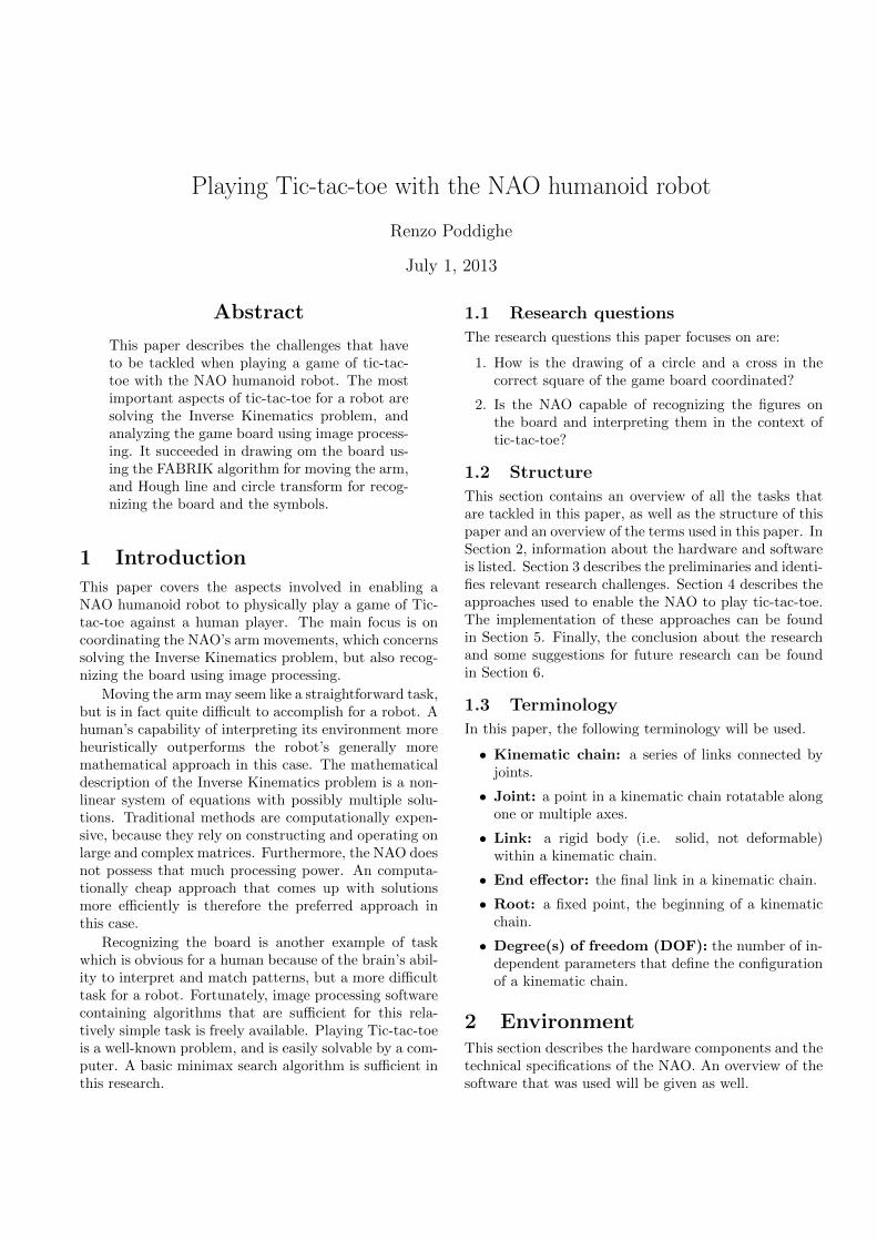
4.2 The FABRIK algorithmFABRIK (short for Forward And Backward ReachingInverse Kinematics) is a novel heuristic method, devel-oped by Aristidou and Lasenby[3], that tackles the In-verse Kinematics problem described in Section 3.2. Un-like traditional methods, FABRIK does not make useof calculations involving matrices or rotational angles.Instead, the IK problem is solved by finding the jointcoordinates as being points on a line. These points areiteratively adjusted one at a time, until the end effec-tor has reached the target position, or the error is suffi-ciently small. FABRIK starts at the end effector of thechain and works forwards, adjusting each joint along theway. Thereafter, it works backwards in the same way, inorder to complete a full iteration. Since the use of rota-tional angles and matrices is avoided, the algorithm haslow computational cost, converges quickly, and does notsuffer from singularity problems. Furthermore, the algo-rithm produces realistic human-like poses and is easilyimplemented.

Algorithm 1 describes the FABRIK algorithm inpseudo-code. In Figure 2, a visualization of the algo-rithm is shown. The various steps of the algorithm, in-dicated with the letters (a) through (f) in Figure 2, aredescribed in words below.

Since homogeneous coordinates are only used in For-ward Kinematics, the n joint positions of the kinematicchain can be represented by the triplets pi = (xi, yi, zi)for i = 1, 2, ..., n, where p1 is the root joint and pn theend effector (a). The target position is named t andthe initial root position is named b. The target posi-tion is reachable if the distance between the root jointand the target position, denoted as dist, is smaller thanor equal to the sum of the distances between the jointsdi = |pi+1 − pi| for i = 1, 2, ..., n − 1. If the target isreachable, the first stage of the algorithm starts. In thisstage, named ’forward reaching’, the joint positions areestimated by positioning the end effector on the targetposition t (b). The new position of the n − 1th joint,p′n−1, lies on the line ln−1, which passes through thepoint pn−1 and the new end effector position p′n, andhas distance dn−1 from p′n (c). Subsequently, the newjoint position p′n−2 can be calculated by taking the pointon the line ln−1 with distance dn−2 from p′n−1. The firststage of the algorithm is completed when all new joint

4

positions have been calculated (d). The current esti-mate is not a feasible one, though, since the position ofthe root has changed. Therefore, a second stage of thealgorithm is necessary to achieve a solution. This stage,named ’backward reaching’, is similar to the first stageof the algorithm, only the operations are carried out theother way around: from the root to the end effector.The new root position p′′1 is the initial root position b(e). The next joint position p′′2 is then determined bytaking the point on the line l1, that passes through thepoints p′′1 and p′2, with distance d1 from p′′1 . This proce-dure is repeated for all other joints, and a full iteration iscomplete (f). The end effector is now closer to its targetposition. The algorithm is repeated until the end effec-tor has reached its target, or the distance to the targetis smaller than a user-defined threshold.

4.3 Calculating back to jointcoordinates

The FABRIK algorithm provides a solution to the in-verse kinematics of the arm, by giving the Cartesian co-ordinates of each joint relative to the root joint. How-ever, the NAO needs to know the joint configurationscorresponding to these coordinates. A mapping from theCartesian coordinates to joint configurations is thereforenecessary in order to make the NAO move its arm.

Recall the three rotation matrices and the translationmatrix from Section 3.1:

Rx(θ) =

1 0 0 00 cos θ − sin θ 00 sin θ cos θ 00 0 0 1

Ry(θ) =

cos θ 0 sin θ 0

0 1 0 0− sin θ 0 cos θ 0

0 0 0 1

Rz(θ) =

cos θ − sin θ 0 0sin θ cos θ 0 0

0 0 1 00 0 0 1

Tr(t) =

1 0 0 tx0 1 0 ty0 0 1 tz0 0 0 1

(8)

Assume that the FABRIK algo-rithm outputs the three joint coordinates(0, 0, 0, 1), (x1, y1, z1, 1), (x2, y2, z2, 1) to be the so-lution to the inverse kinematics problem for a targetposition t = (x2, y2, z2, 1). Equation 9 describes theforward kinematics equation for mapping from the firsttwo (currently unknown) rotations θ1 and θ2 to thesecond joint coordinate p1:

Algorithm 1 The FABRIK algorithm.

Input: The joint positions pi for i = 1, ..., n, the targetposition t and the distances between each joint di =|pi+1 − pi| for i = 1, ..., n− 1.

Output: The new joint positions pi for i = 1, ..., n.% The distance between root and targetdist = |p1 − t|% Check whether the target is within reachif dist >= d1 + d2 + ...+ dn−1 then

% The target is unreachablefor i = 1, ..., n− 1 do

% Find the distance ri between the target t andthe joint position piri = |t− pi|λi = di/ri% Find the new joint positions pipi+1 = (1− λi)pi + λit

end forelse

% The target is reachable; thus, set b as the initialposition of the joint p1b = p1% Check whether the distance between the end effec-tor pn and the target t is greater than a tolerancedifA = |pn − t|while difA > tol do

% STAGE 1: FORWARD REACHING% Set the end effector pn as target tpn = tfor i = n-1, ..., 1 do

% Find the distance ri between the new jointposition pi+1 and the joint piri = |pi+1 − pi|λi = di/ri% Find the new joint positions pipi = (1− λi)pi+1 + λipi

end for% STAGE 2: BACKWARD REACHING% Set the root p1 at its initial positionp1 = bfor i = 1, ..., n-1 do

% Find the distance ri between the new jointposition pi and the joint pi+1

λi = di/ri% Find the new joint positions pipi+1 = (1− λi)pi + λipi+1

end fordifA = |pn − t|

end whileend if

5

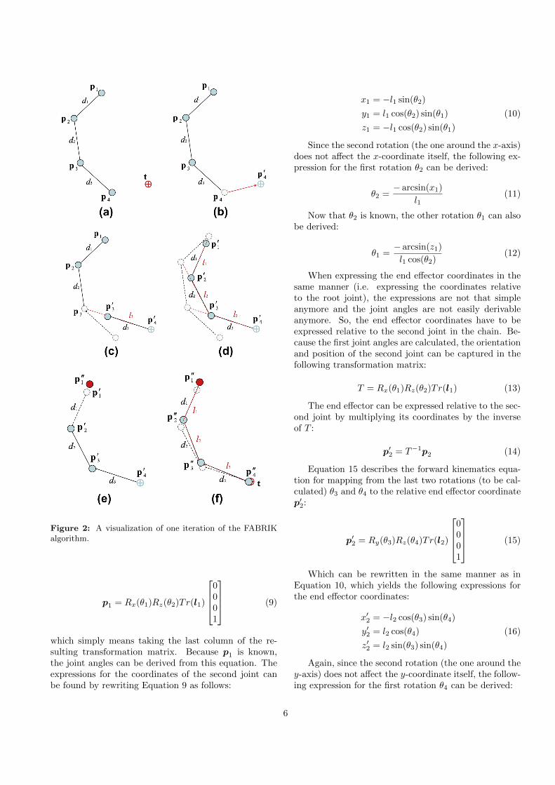
Figure 2: A visualization of one iteration of the FABRIKalgorithm.

p1 = Rx(θ1)Rz(θ2)Tr(l1)

0001

(9)

which simply means taking the last column of the re-sulting transformation matrix. Because p1 is known,the joint angles can be derived from this equation. Theexpressions for the coordinates of the second joint canbe found by rewriting Equation 9 as follows:

x1 = −l1 sin(θ2)

y1 = l1 cos(θ2) sin(θ1)

z1 = −l1 cos(θ2) sin(θ1)

(10)

Since the second rotation (the one around the x-axis)does not affect the x-coordinate itself, the following ex-pression for the first rotation θ2 can be derived:

θ2 =− arcsin(x1)

l1(11)

Now that θ2 is known, the other rotation θ1 can alsobe derived:

θ1 =− arcsin(z1)

l1 cos(θ2)(12)

When expressing the end effector coordinates in thesame manner (i.e. expressing the coordinates relativeto the root joint), the expressions are not that simpleanymore and the joint angles are not easily derivableanymore. So, the end effector coordinates have to beexpressed relative to the second joint in the chain. Be-cause the first joint angles are calculated, the orientationand position of the second joint can be captured in thefollowing transformation matrix:

T = Rx(θ1)Rz(θ2)Tr(l1) (13)

The end effector can be expressed relative to the sec-ond joint by multiplying its coordinates by the inverseof T :

p′2 = T−1p2 (14)

Equation 15 describes the forward kinematics equa-tion for mapping from the last two rotations (to be cal-culated) θ3 and θ4 to the relative end effector coordinatep′2:

p′2 = Ry(θ3)Rz(θ4)Tr(l2)

0001

(15)

Which can be rewritten in the same manner as inEquation 10, which yields the following expressions forthe end effector coordinates:

x′2 = −l2 cos(θ3) sin(θ4)

y′2 = l2 cos(θ4)

z′2 = l2 sin(θ3) sin(θ4)

(16)

Again, since the second rotation (the one around they-axis) does not affect the y-coordinate itself, the follow-ing expression for the first rotation θ4 can be derived:

6

θ4 =− arccos(y′2)

l2(17)

after which the last rotation θ3 can be derived as well:

θ3 =− arcsin(z′2)

l2 sin(θ4)(18)

4.4 Hough line transform

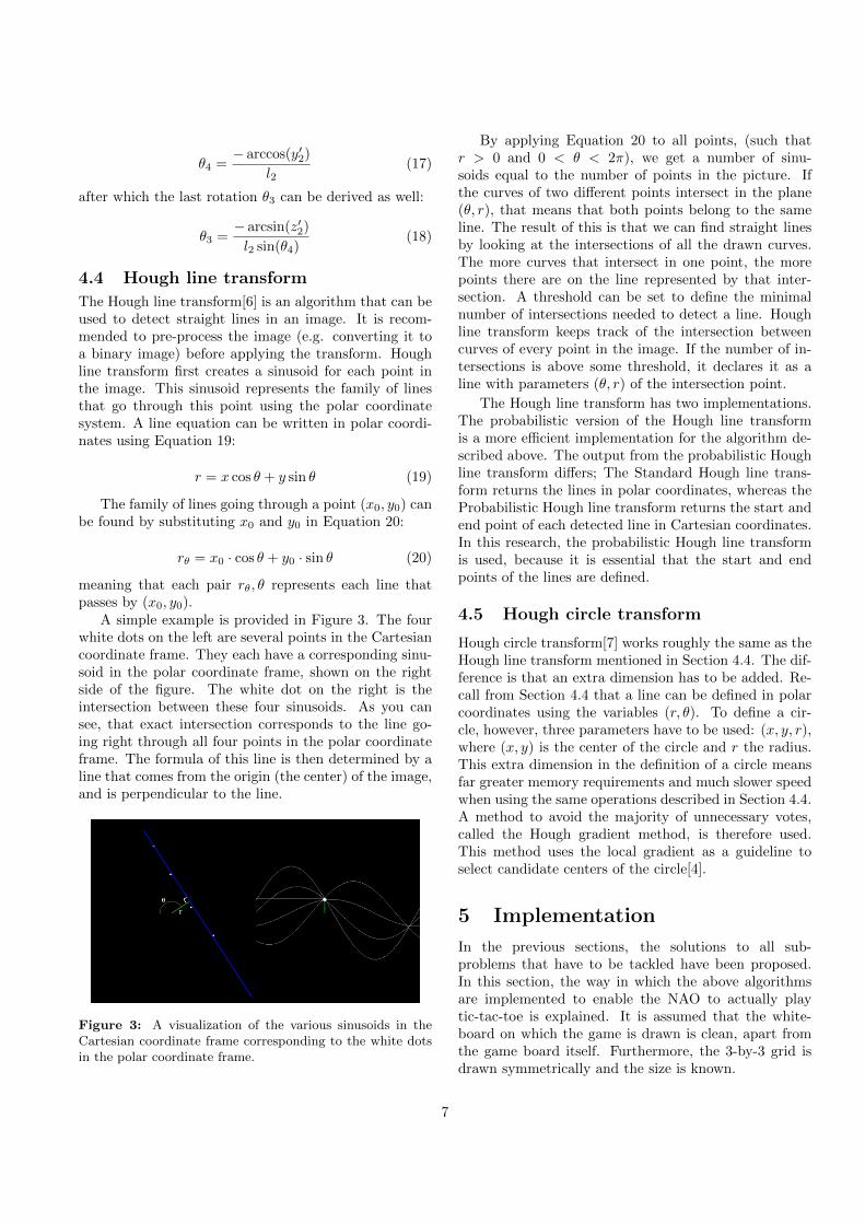
The Hough line transform[6] is an algorithm that can beused to detect straight lines in an image. It is recom-mended to pre-process the image (e.g. converting it toa binary image) before applying the transform. Houghline transform first creates a sinusoid for each point inthe image. This sinusoid represents the family of linesthat go through this point using the polar coordinatesystem. A line equation can be written in polar coordi-nates using Equation 19:

r = x cos θ + y sin θ (19)

The family of lines going through a point (x0, y0) canbe found by substituting x0 and y0 in Equation 20:

rθ = x0 · cos θ + y0 · sin θ (20)

meaning that each pair rθ, θ represents each line thatpasses by (x0, y0).

A simple example is provided in Figure 3. The fourwhite dots on the left are several points in the Cartesiancoordinate frame. They each have a corresponding sinu-soid in the polar coordinate frame, shown on the rightside of the figure. The white dot on the right is theintersection between these four sinusoids. As you cansee, that exact intersection corresponds to the line go-ing right through all four points in the polar coordinateframe. The formula of this line is then determined by aline that comes from the origin (the center) of the image,and is perpendicular to the line.

Figure 3: A visualization of the various sinusoids in theCartesian coordinate frame corresponding to the white dotsin the polar coordinate frame.

By applying Equation 20 to all points, (such thatr > 0 and 0 < θ < 2π), we get a number of sinu-soids equal to the number of points in the picture. Ifthe curves of two different points intersect in the plane(θ, r), that means that both points belong to the sameline. The result of this is that we can find straight linesby looking at the intersections of all the drawn curves.The more curves that intersect in one point, the morepoints there are on the line represented by that inter-section. A threshold can be set to define the minimalnumber of intersections needed to detect a line. Houghline transform keeps track of the intersection betweencurves of every point in the image. If the number of in-tersections is above some threshold, it declares it as aline with parameters (θ, r) of the intersection point.

The Hough line transform has two implementations.The probabilistic version of the Hough line transformis a more efficient implementation for the algorithm de-scribed above. The output from the probabilistic Houghline transform differs; The Standard Hough line trans-form returns the lines in polar coordinates, whereas theProbabilistic Hough line transform returns the start andend point of each detected line in Cartesian coordinates.In this research, the probabilistic Hough line transformis used, because it is essential that the start and endpoints of the lines are defined.

4.5 Hough circle transform

Hough circle transform[7] works roughly the same as theHough line transform mentioned in Section 4.4. The dif-ference is that an extra dimension has to be added. Re-call from Section 4.4 that a line can be defined in polarcoordinates using the variables (r, θ). To define a cir-cle, however, three parameters have to be used: (x, y, r),where (x, y) is the center of the circle and r the radius.This extra dimension in the definition of a circle meansfar greater memory requirements and much slower speedwhen using the same operations described in Section 4.4.A method to avoid the majority of unnecessary votes,called the Hough gradient method, is therefore used.This method uses the local gradient as a guideline toselect candidate centers of the circle[4].

5 Implementation

In the previous sections, the solutions to all sub-problems that have to be tackled have been proposed.In this section, the way in which the above algorithmsare implemented to enable the NAO to actually playtic-tac-toe is explained. It is assumed that the white-board on which the game is drawn is clean, apart fromthe game board itself. Furthermore, the 3-by-3 grid isdrawn symmetrically and the size is known.

7

Figure 4: A picture of a tic-tac-toe board before and afterline and circle detection. The detected lines and circles aredrawn on top of the original image.

5.1 Processing the boardThere are several types of information that have to begathered from the board. Image processing is importantfor analyzing the state of the game so that the next movecan be determined, and subsequently for determining theposition to which the arm has to move next.

Analyzing the state of the game

In order to determine the next move, the state of thegame has to be retrieved from the board. The game statecan be represented by an array of nine entries, each ofwhich is filled with a 0 if it is empty, a 1 if it contains across and a 2 if it contains a circle. Before analyzing theimage, it is first preprocessed by a built-in OpenCV func-tion inRange(). This function converts the image intoa binary image, replacing a pixel by a 1 if it lies in thespecified color range, and 0 otherwise. The algorithmsmentioned in Section 4, the Hough line and Hough cir-cle transform, are then used to find all lines and circlesin the image. The image can be split up in 9 segmentsusing the minimum and maximum x- and y-coordinates

of the found lines. Then, for each found line, it can bechecked whether the line falls into one of the segments.This is done by checking if the start and end coordinatesof the line do so. If they do, the corresponding array en-try is filled with a 1. In the same manner, for each foundcircle, it can be checked whether the circle falls into oneof the segments by checking if the center of the circledoes. If it does, the array entry is filled with a 2. Whenthe array matches the game state, it can be processedby a minimax algorithm to determine the next move.

Calculating the coordinates

As explained in Section 4.2, FABRIK can be used tomake the end effector of the NAO’s arm move to a de-sired position in Cartesian space. In order for the NAOto be able to do this, however, the pixel coordinates firsthave to be converted to Cartesian coordinates. Sincethe size of the board is known, calculating the x- and y-coordinates is simple. The magnification M of the imagecan be found by:

M =X

x(21)

where X is the actual width of the board and x thewidth of the projected board in pixels. The x- and ycoordinates can then be calculated as follows:

x = Mx′

y = My′(22)

where x′ and y′ are the desired pixel coordinates the armneeds to move to.

The z-coordinate equals the distance d to the board.To know the relation between the distance of the boardand the pixel size of the image, for instance, the focallength of the camera has to be calculated. This can bedone by placing the NAO at a known distance d from theboard, taking an image, and measuring the pixel width xof the board. The focal length f can then be calculatedas follows:

f = x× d

X(23)

where X is the actual width of the board. The distanceto the board d can now be calculated as follows:

d = X × f

x(24)

5.2 Drawing a crossOnce the coordinates of the target square are known,moving the NAO’s arm is not difficult. In order for theNAO to be able to draw, it needs to slightly press the penagainst the board. To do this, simply lower the stiffnessof the arm to make it more flexible, and set the targetslightly behind the board. The NAO starts its drawing

8

at the top left of the square. The first diagonal line cannow be drawn by making the arm move to a target at thebottom right of the square. The pen then has to be liftedfrom the board, by slightly adjusting the z-coordinate.Finally, the NAO moves its arm to the top right, pressesthe pen onto the board again, and then draws a similarline to the bottom left. To make the lines more straight,several intermediate targets can be set. So, a simpletrajectory can be created by simply specifying targets inthe direction the arm needs to move.

6 ConclusionThe proposed methods in this paper have dealt withthe challenging subproblems - solving Inverse Kinematicsand processing the game board - that arise when playingtic-tac-toe with the NAO. Using image processing, theNAO could analyze the game state, and make a decisionbased on that. Executing the decision implies drawinga cross on the board, which requires solving an inversekinematic problem. The new algorithm FABRIK has alot of advantages over traditional methods for solving aninverse kinematic problem: it is very accurate, convergesquickly, and is well-behaved for every reachable point inspace. Using this algorithm, the NAO was able to letits hand follow a trajectory, which results in drawing across on the board.

Future research

There is still room for improvement. The NAO’s armhas a very limited range. The program can be mademore flexible by increasing the space in which the NAOcan draw. This can be done by involving the rest ofthe body in the drawing. For instance, walking alongthe board to increase the horizontal range, or using itsknees to increase the vertical range. The NAO wouldthen be able to play on a bigger game board.

Another improvement could be to provide some kindof feedback about the amount of pressure the NAO ap-plies to the marker. If this can be kept constant, it canresult in smoother drawings and more straight lines.

References[1] (2013). Aldebaran Robotics.

http://www.aldebaran-robotics.com.

[2] Aldebaran Robotics (2013).qibuild 1.14 documentation.http://www.aldebaran-robotics.com/documentation.

[3] Aristidou, Andreas and Lasenby, Joan (2011).Fabrik: A fast, iterative solver for the inversekinematics problem. Graphical Models.

[4] Bradski, Gary and Kaehler, Adrian (2008).Learning OpenCV: Computer Vision with theOpenCV Library. O’Reilly Media.

[5] (2013). Eigen. http://eigen.tuxfamily.org/.

[6] OpenCV Development Team (2011).Opencv 2.3.1 documentation.http://docs.opencv.org/2.3/modules/refman.html.

[7] OpenCV Development Team (2012). Hough circletransform. http://docs.opencv.org.

[8] Paul, Richard P. (1981). Robot Manipulators:Mathematics, Programming, and Control. MITPress.

[9] Russell, Stuart and Norvig, Peter (2009). Artifi-cial Intelligence: A Modern Approach. PrenticeHall, third edition.

9