Plant breeding with farmers - orgprints.orgorgprints.org/32587/17/techmanual_ceccarelli.pdf ·...
139
-
Upload
trinhquynh -
Category
Documents
-
view
227 -
download
0
Transcript of Plant breeding with farmers - orgprints.orgorgprints.org/32587/17/techmanual_ceccarelli.pdf ·...
Plant breeding with farmers A technical manual
International Center for Agricultural Research in the Dry Areas
2012
S. Ceccarelli

Copyright © 2012 International Center for Agricultural Research in the Dry Areas (ICARDA) All rights reserved. ICARDA encourages fair use of this material for non-commercial purposes, with proper citation. The opinions expressed are those of the author, not necessarily those of ICARDA. Where trade names are used, it does not imply endorsement of, or discrimination against, any product by ICARDA.
Citation: Ceccarelli, S. 2012. Plant breeding with farmers – a technical manual. ICARDA, PO Box 5466, Aleppo, Syria. pp xi + 126.
ISBN 92-9127-271-X
Various software tools are referred to in this manual:ALPHANAL © Scottish Crop Research Institute.GenStat © VSN International.GGEbiplot was developed by Dr Weikai Yan, who gave authorization to reproduce parts of the product in descriptions in the manual.DiGGer was developed by Dr Neil Coombes and is freely available on the Web.

iii
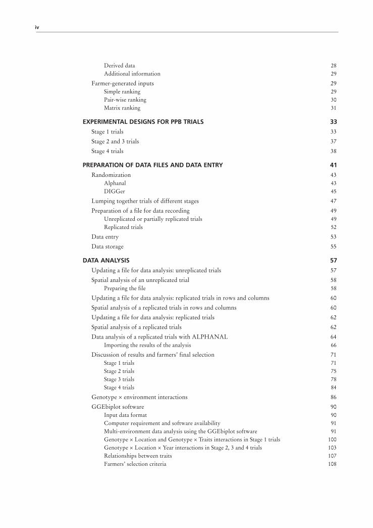
Contents
Foreword viiAcknowledgement viiiAbbreviations used in the text ixExecutive summary xi
INTRODUCTION AND DEFINITIONS 1
Historical perspective 1
Plant breeding 3Self-pollinated crops 5Cross-pollinated crops 5Vegetatively propagated crops 6
Who is a plant breeder? 6
Participatory Plant Breeding (PPB) 6
Participatory Variety Selection (PVS) 9
A general model of participatory plant breeding 9
Decentralized plant breeding 12
HOW TO GET STARTED: ORGANIZATIONAL ISSUES 13
Setting criteria to identify target environments and target users 15
Choice of the target environment and users 16
Type of participation 18
Choice of genetic material 18
Choice of parental material 18
Choice of breeding method 19
When farmer participation should start 20
Naming of varieties 20
Management of trials in farmers’ fields 21
Managing equipment 21
Farmer selection 23
Visits to farmers 24
Managing the transition phase 24
Sharing and disseminating findings 26
DATA COLLECTION 27
Traditional approach 27
Digital approach 27
Parameters recorded 28Before harvesting 28At harvest 28After harvest 28
iv
Derived data 28Additional information 29
Farmer-generated inputs 29Simple ranking 29Pair-wise ranking 30Matrix ranking 31
EXPERIMENTAL DESIGNS FOR PPB TRIALS 33
Stage 1 trials 33
Stage 2 and 3 trials 37
Stage 4 trials 38
PREPARATION OF DATA FILES AND DATA ENTRY 41
Randomization 43Alphanal 43DIGGer 45
Lumping together trials of different stages 47
Preparation of a file for data recording 49Unreplicated or partially replicated trials 49Replicated trials 52
Data entry 53
Data storage 55
DATA ANALYSIS 57
Updating a file for data analysis: unreplicated trials 57
Spatial analysis of an unreplicated trial 58Preparing the file 58
Updating a file for data analysis: replicated trials in rows and columns 60
Spatial analysis of a replicated trials in rows and columns 60
Updating a file for data analysis: replicated trials 62
Spatial analysis of a replicated trials 62
Data analysis of a replicated trials with ALPHANAL 64Importing the results of the analysis 66
Discussion of results and farmers’ final selection 71Stage 1 trials 71Stage 2 trials 75Stage 3 trials 78Stage 4 trials 84
Genotype × environment interactions 86
GGEbiplot software 90Input data format 90Computer requirement and software availability 91Multi-environment data analysis using the GGEbiplot software 91Genotype × Location and Genotype × Traits interactions in Stage 1 trials 100Genotype × Location × Year interactions in Stage 2, 3 and 4 trials 103Relationships between traits 107Farmers’ selection criteria 108

v
VARIETY RELEASE AND SEED PRODUCTION 111
THE IMPACT OF PLANT BREEDING 115
Conventional plant breeding 115
Participatory plant breeding 116
CONCLUSIONS 119
REFERENCES 121

"… there is nothing more difficult to arrange, more doubtful of success, more dangerous to carry through than initiating changes...The innovator makes enemies of all those who prosper under the old order, and only lukewarm support is forthcoming from those who would prosper under the new. Men are generally incredulous, never really trusting new things unless they have tested them by experience."
Nicholas Machiavelli, 1513
vii
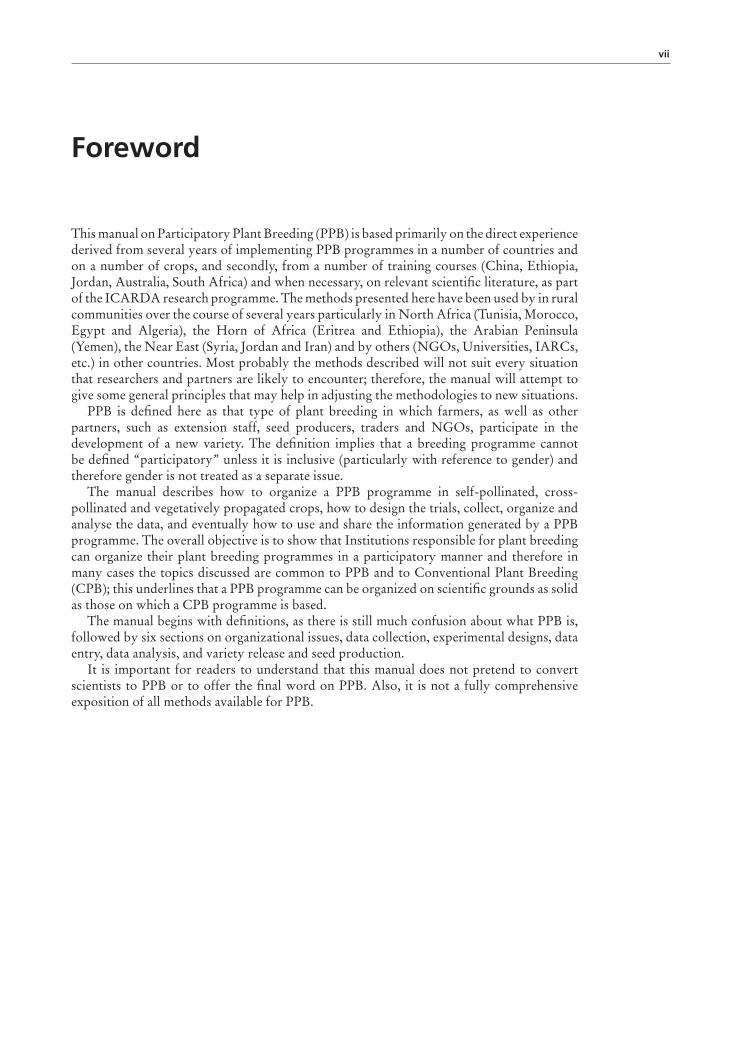
Foreword
This manual on Participatory Plant Breeding (PPB) is based primarily on the direct experience derived from several years of implementing PPB programmes in a number of countries and on a number of crops, and secondly, from a number of training courses (China, Ethiopia, Jordan, Australia, South Africa) and when necessary, on relevant scientific literature, as part of the ICARDA research programme. The methods presented here have been used by in rural communities over the course of several years particularly in North Africa (Tunisia, Morocco, Egypt and Algeria), the Horn of Africa (Eritrea and Ethiopia), the Arabian Peninsula (Yemen), the Near East (Syria, Jordan and Iran) and by others (NGOs, Universities, IARCs, etc.) in other countries. Most probably the methods described will not suit every situation that researchers and partners are likely to encounter; therefore, the manual will attempt to give some general principles that may help in adjusting the methodologies to new situations.
PPB is defined here as that type of plant breeding in which farmers, as well as other partners, such as extension staff, seed producers, traders and NGOs, participate in the development of a new variety. The definition implies that a breeding programme cannot be defined “participatory” unless it is inclusive (particularly with reference to gender) and therefore gender is not treated as a separate issue.
The manual describes how to organize a PPB programme in self-pollinated, cross-pollinated and vegetatively propagated crops, how to design the trials, collect, organize and analyse the data, and eventually how to use and share the information generated by a PPB programme. The overall objective is to show that Institutions responsible for plant breeding can organize their plant breeding programmes in a participatory manner and therefore in many cases the topics discussed are common to PPB and to Conventional Plant Breeding (CPB); this underlines that a PPB programme can be organized on scientific grounds as solid as those on which a CPB programme is based.
The manual begins with definitions, as there is still much confusion about what PPB is, followed by six sections on organizational issues, data collection, experimental designs, data entry, data analysis, and variety release and seed production.
It is important for readers to understand that this manual does not pretend to convert scientists to PPB or to offer the final word on PPB. Also, it is not a fully comprehensive exposition of all methods available for PPB.

viii
Acknowledgement
The author has been a barley breeder at ICARDA, based in Aleppo, Syria, for nearly 30 years. After decentralizing the breeding programme to National Programmes in the early 1990s, his team started PPB in 1996 in Syria, with the financial support of GTZ (Germany). Later PPB was extended to other countries with the support of IDRC (Canada), DANIDA (Denmark), the Governments of Italy and of Switzerland, the Participatory Research and Gender Analysis System-Wide Program (PRGA) of the CGIAR, the Global Crop Diversity Trust, the OPEC Fund for International Development, IFAD and the CGIAR Challenge Programme on Water and Food. During the preparation of the manuscript the author has been partly supported by the SOLIBAM project.
The author gratefully acknowledges the contribution of several national programme scientists and of very many farmers, the support of policy-makers in Algeria, Eritrea, Islamic Republic of Iran, Jordan and Yemen, and the encouragement and positive cooperation of many scientists. In particular, I would like to acknowledge the suggestions of J. Dawson, M. Maatougui, A. Galié, S. Grando, M. Singh, W. Yan, M. Wirthensohn, S. Rosenfeld, D. Kassahun Mengistu, H. Giraud and Y. Song.
This publication reports on a research project financed by Canada's International Development Research Centre (www.idrc.ca).
ix
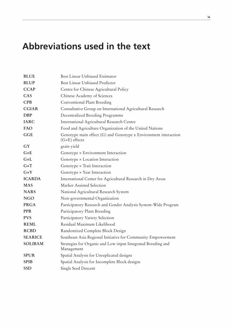
Abbreviations used in the text
BLUE Best Linear Unbiased Estimator
BLUP Best Linear Unbiased Predictor
CCAP Centre for Chinese Agricultural Policy
CAS Chinese Academy of Sciences
CPB Conventional Plant Breeding
CGIAR Consultative Group on International Agricultural Research
DBP Decentralized Breeding Programme
IARC International Agricultural Research Centre
FAO Food and Agriculture Organization of the United Nations
GGE Genotype main effect (G) and Genotype x Environment interaction (G×E) effects
GY grain yield
G×E Genotype × Environment Interaction
G×L Genotype × Location Interaction
G×T Genotype × Trait Interaction
G×Y Genotype × Year Interaction
ICARDA International Center for Agricultural Research in Dry Areas
MAS Marker Assisted Selection
NARS National Agricultural Research System
NGO Non-governmental Organization
PRGA Participatory Research and Gender Analysis System-Wide Program
PPB Participatory Plant Breeding
PVS Participatory Variety Selection
REML Residual Maximum Likelihood
RCBD Randomized Complete Block Design
SEARICE Southeast Asia Regional Initiative for Community Empowerment
SOLIBAM Strategies for Organic and Low-input Integrated Breeding and Management
SPUR Spatial Analysis for Unreplicated designs
SPIB Spatial Analysis for Incomplete Block designs
SSD Single Seed Descent


xi
Executive summary
There is increasing interest in participatory plant breeding (PPB), both in developing and in developed countries. While there is a conspicuous body of literature in the form of both scientific papers and books, this manual aims to provide a source of information on how to implement a PPB programme on the ground, with the purpose of encouraging scientists to start such programmes. The manual is addressed to all those involved in planning and implementing participatory breeding activities. This includes research centres, universities, non-governmental organizations (NGOs), farmer associations and government extension officials
This manual presents some background on PPB and on participatory variety selection (PVS), but is mostly devoted to providing the reader with as much detailed technical information on the different aspects involved in successfully starting and conducting a PPB programme. The manual fills a gap by making available in one document diverse information that is otherwise scattered in several different publications.
The manual shows clearly that there are no major technical difficulties in transforming a conventional breeding programme into a participatory programme. In fact, many of the principles and techniques described in this manual apply equally well to conventional plant breeding programmes. Readers are encouraged to submit their comments, corrections or criticism to improve future versions of the manual.
The objectives of this manual are to:• Introduce the reader to the concepts and methodologies of plant breeding in general,
and to participatory plant breeding in particular;• Take the user through the main steps in designing and implementing participatory
breeding programmes in various crops;• Provide examples of data collection and data analysis for various types of experimental
designs; and • Discuss key issues in participatory plant breeding, such as variety release, seed
production and impact.The manual draws heavily on ICARDA’s experience in conducting participatory breeding
programmes in Algeria, Egypt, Eritrea, Ethiopia, Iran, Jordan, Morocco, Syria, Tunisia and Yemen. However, efforts have been made to highlight a number of general principles that entitle a research programme to be called “participatory”.
Inputs and perspectives from interested readers are welcome.Contact: [email protected] or [email protected]

1
Introduction and definitions
HISTORICAL PERSPECTIVEIn recent years there has been increasing interest toward participatory research in general, and toward participatory plant breeding (PPB) in particular. Following the early work of Rhoades and Booth (1982), scientists have become increasingly aware that user participation in technology development may substantially increase the probability of adoption of the technology.
That farmers should be involved in plant breeding was recognized over a century ago. In 1908 a Bulletin of Cornell University stated
“To every farmer the field of breeding, whether in plants or animals, furnishes an interesting and profitable diversion. Plant breeding especially should become a farmer’s fad. Few can afford to breed animals in the extensive way necessary to secure important results, owing to the expense. No farmer, however, is so poor but that he can have his breeding patch of corn, wheat or potatoes. Indeed, if they but knew it, they can ill afford not to have such a breeding patch to furnish seed for their own planting.” (Webber, 1908). The more recent interest is partly associated with the perception that the impact of
agricultural research, including plant breeding, has been below expectations, particularly in developing countries, and for marginal environments and poor farmers. In fact, about 2 billion people still lack reliable access to safe, nutritious food (Reynolds and Borlaug, 2006), and more than one billion suffer from food insecurity and malnutrition (IAASTD, 2009). More recent data (Foresight, 2011) indicate that hunger remains widespread, with 925 million people experiencing hunger: they lack access to sufficient of the major macronutrients (carbohydrates, fats and protein). Perhaps another billion are thought to suffer from ‘hidden hunger’, in which important micronutrients (such as vitamins and minerals) are missing from their diet, with consequent risks of physical and mental impairment. In contrast, a billion people are substantially over-consuming, spawning a new public health epidemic involving chronic conditions such as type 2 diabetes and cardiovascular disease. Much of the responsibility for these three billion people having suboptimal diets lies within the global food system, which in turn is affected by the decreased agro biodiversity and by climate changes.
The main rationale for PPB and participatory varietal selection (PVS) in developing-country agriculture is the existence of important cropping systems in marginal regions where the adoption of modern varieties is low or negligible (Walker, 2007). This widespread perception that the green-revolution varieties have had an impact only on irrigated areas of high production potential is not strictly correct, as farmers in large regions of rainfed agriculture have benefited from varietal change. For instance, improved wheat varieties have penetrated many so-called marginal production regions in Asia and Latin America (Byerlee, 1994). Moreover, not all high-potential regions are characterized by a rapid turnover of improved varieties; in some high-yielding areas of South Asia, farmers still grow varieties that were bred more than 40 years ago.
But, in general, the conventional wisdom of by-passed marginal regions that have not benefited from modern varieties still prevails. One can document extensive tracts where the adoption of improved varieties is effectively nil, even in countries with strong national agricultural research programmes. In India, post-rainy season sorghum is a cropping system
Plant breeding with farmers – a technical manual2
that seamlessly fits the description of a by-passed region (Walker and Ryan, 1990). The dominant sorghum variety in post-rainy season is still Maldandi (M 35-1), an improved local selection released by the Sholapur research station in 1933 (B.S. Dhillon, pers. comm., 2006, quoted by Walker, 2007). And, Maldandi excels in several key traits, such as grain colour and size, fodder production, drought tolerance and pest resistance (Dvorak, 1987). Still, the absence of progress in stimulating varietal change in a cropping system covering several million hectares in a strong NARS setting is surprising.
As we will see in the section on Genotype × Environment (G×E) Interactions the main reason for the limited impact of plant breeding in marginal environments is the existence of large interactions (i.e. differences) among the performances of breeding materials, which varies from research stations (the selection environment) to the field of poor farmers or in marginal areas (the target environment). When the magnitude of these G×E interactions is such that the ranking of varieties changes, then selection on research stations will not result in the expected response to selection in the target environment.
PPB has evolved mainly to address the difficulties of poor farmers in developing countries. Widely seen as having advantages for use in low yield potential, high stress environments, PPB is most often applied when specific adaptation is sought. For this reason, a review of plant breeding methodologies in the CGIAR conducted in 2001 recommended that it should form an “organic part of each Center’s breeding programme” (TAC, 2001: 24). However, some results show that both specific and wide adaptation is possible (see for example, Joshi, Sthapit and Witcombe, 2001).
Three common characteristics of most agricultural research programmes that might help explain its limited impact in marginal areas are:
• The research agenda is usually decided unilaterally by the scientists and is not discussed with the user.
• Agricultural research is typically organized in compartments, that is, disciplines and/or commodities (for example breeding and agronomy, or breeding programmes of specific crops), and seldom uses an integrated approach; this contrasts with the integration existing at farm level.
• There is a disproportional development between the large number of technologies generated by the agricultural scientists and the relatively small number of them actually adopted and used by the farmers.
When one looks at these characteristics as applied to plant breeding programmes, most scientists would agree that:
1. Plant breeding has not been very successful in marginal environments and for poor farmers.2. It still takes a long time (about 15 years) to develop and release a new variety,
particularly in developing countries.3. Many varieties are officially released, but few are adopted by farmers; despite the
release of nearly 1700 improved wheat varieties in developing countries during the period 1988–2002 (Lantican, Dubin and Morris, 2005), only a relatively small number have been adopted on a substantial scale by farmers (Smale et al., 2002). In Ethiopia, for example, over 122 varieties of cereals, legumes and vegetables have been released, but only 12 varieties had been adopted by farmers (Mekbib, 1997), and similar examples are known in many countries. In contrast, farmers often grow varieties that have not been officially released, a phenomenon known to be associated not only with an inefficient and biased testing system prior to variety release, but also with breeders using different selection criteria from the farmers and particularly G×E interactions in the case of farmers in marginal environments (see page 86).
4. Even when new varieties are acceptable to farmers, the seed is either not available or too expensive.
Introduction and definitions 3
5. There is a widespread perception of a decrease of biodiversity associated with conventional plant breeding (CPB) programmes.
Participatory research is defined in general as that type of research in which users are involved in the design – and not merely in the final testing – of a new technology. PPB, in particular, is that type of plant breeding in which farmers, as well as other partners, such as extension staff, seed producers, traders and NGOs, participate and collaborate in the development of a new variety.
Participatory research is now seen by many as a way to address the problems noted above, as PPB is expected to produce varieties that are targeted (focused on various typologies of partners), relevant (responding to real needs, concerns and preferences) and appropriate (able to produce results that can be adopted) (Bellon, 2006).
The objective of this manual is to illustrate some of the characteristics of PPB using mostly, but non exclusively, examples from projects implemented in a number of countries by the International Center for Agricultural Research in the Dry Areas (ICARDA).
In several sections the Manual draws on a recently published book: Plant Breeding and Farmer Participation (Ceccarelli, Guimaraes and Weltzien, 2009).
There are many definitions of PPB, reflecting the fact that many PPB practitioners are not plant breeders, and therefore we will start this manual by defining plant breeding in general and PPB in particular.
PLANT BREEDINGPlant breeding is an applied, multidisciplinary science based on the application of genetic principles and practices for the development of cultivars more suited to the needs of people; it uses knowledge from agronomy, botany, genetics, cytogenetics, molecular genetics, physiology, pathology, entomology, biochemistry, bio-informatics and statistics (Schlegel, 2003). The ability to transfer, in addition to major genes, large suites of genes conditioning quantitative traits such as yield and other traits of socio-economic interest is of particular importance. The ultimate outcome of plant breeding is mainly improved cultivars. Therefore, plant breeding is primarily a science which looks at the organism as a whole even though it is also suited to translate information at the molecular level (DNA sequences, protein products) into economically important phenotypes (Gepts and Hancock, 2006).
As a science, plant breeding started soon after the rediscovery of Mendel’s Laws at the beginning of the 20th century. Before that, plant improvement had been done for several thousand years by farmers who, after domesticating the crops which give the food, feed, medicines, textiles, etc., of today, have continued to modify them, and to move them from continent to continent, adapting them to new climates, new cultural practices and new uses. There is evidence that hybridization also started before 1900 (as discussed by, for example, Strampelli, 1944).
Since then, plant breeding has evolved by absorbing approaches from different areas of science, allowing breeders to increase their efficiency and exploit genetic resources more thoroughly (Gepts and Hancock, 2006). Over the years, it has put to productive use progress in crop evolution, population and quantitative genetics, statistical genetics and biometry, molecular biology, and genomics. Thus, plant breeding has remained a vibrant science, with continued success in developing and deploying new cultivars on a worldwide basis. On average, around 50% of productivity increases can be attributed to genetic improvement (Fehr, 1984).
Despite differences between crops and between breeders, in all breeding programmes it is possible to identify three main stages (Schnell, 1982; Ceccarelli, 2009a):
1. Generating genetic variability. This includes making crosses (selection of parents, crossing techniques and type of crosses), inducing mutation, and introducing exotic germplasm.
Plant breeding with farmers – a technical manual4
2. Selection of the best genetic material within the genetic variability created in the first stage. In self-pollinated crops this includes primarily the implementation of various methods, such as classical pedigree, bulk pedigree, backcross, hybridisation, recurrent selection, or the F2 progeny method. In self-pollinated tree crops this includes progressive evaluation of individual plants. In cross-pollinated crops, synthetic varieties, open pollinated varieties and hybrids are used, and in vegetatively propagated crops there are clones and hybrids. Marker assisted selection (MAS) could be used in this stage.
3. Testing of breeding lines. This includes comparisons between existing cultivars and the breeding lines emerging from Stage 2, and the appropriate methodologies to conduct such comparisons. These comparisons take place partly on-station (on-station trials) and partly in farmers’ fields (on-farm trials).
As a consequence of Stage 1 and partly also due to selection during the first part of Stage 2, the amount of breeding materials generated is very large (from a few to several thousands). During Stages 2 and 3 the number of breeding lines decreases, the amount of seed per line increases and so does the number of locations where the material can be tested.There are two other important stages in a breeding programme: setting priorities; and dissemination of cultivars. These two steps have been discussed in detail by Weltzien and Christinck (2009) and by Bishaw and van Gastel (2009).
In a CPB programme (i.e. non-participatory) all the decisions are taken by the breeder and by the breeding team, even in the case of on-farm trials.
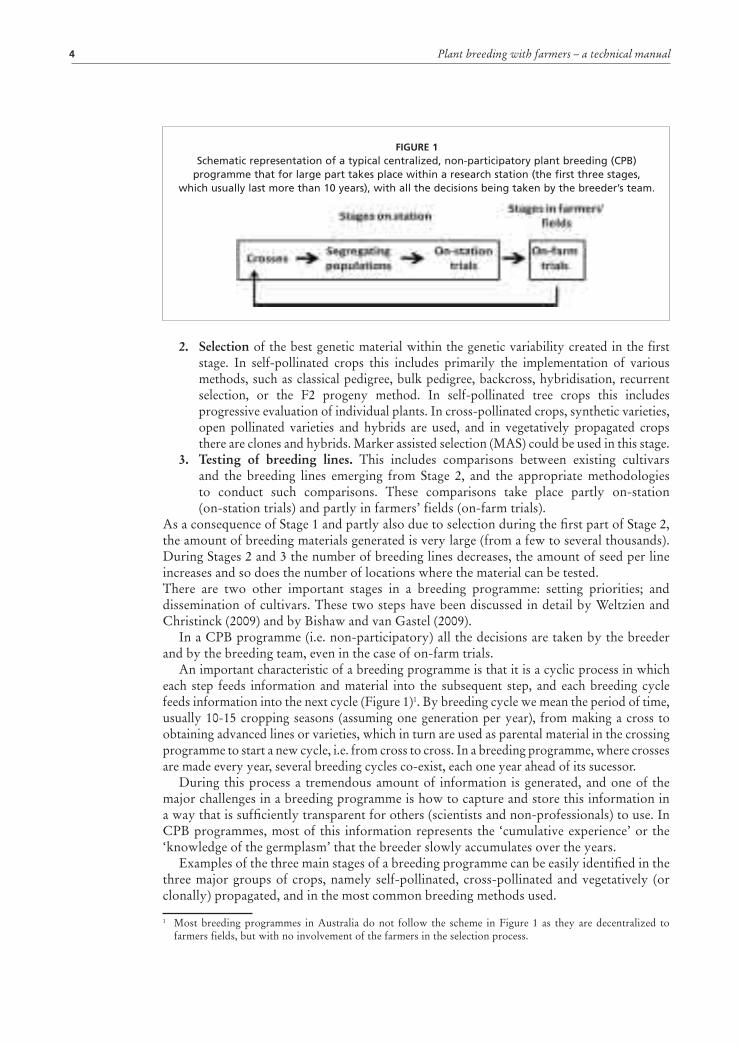
An important characteristic of a breeding programme is that it is a cyclic process in which each step feeds information and material into the subsequent step, and each breeding cycle feeds information into the next cycle (Figure 1)1. By breeding cycle we mean the period of time, usually 10-15 cropping seasons (assuming one generation per year), from making a cross to obtaining advanced lines or varieties, which in turn are used as parental material in the crossing programme to start a new cycle, i.e. from cross to cross. In a breeding programme, where crosses are made every year, several breeding cycles co-exist, each one year ahead of its sucessor.
During this process a tremendous amount of information is generated, and one of the major challenges in a breeding programme is how to capture and store this information in a way that is sufficiently transparent for others (scientists and non-professionals) to use. In CPB programmes, most of this information represents the ‘cumulative experience’ or the ‘knowledge of the germplasm’ that the breeder slowly accumulates over the years.
Examples of the three main stages of a breeding programme can be easily identified in the three major groups of crops, namely self-pollinated, cross-pollinated and vegetatively (or clonally) propagated, and in the most common breeding methods used.
1 Most breeding programmes in Australia do not follow the scheme in Figure 1 as they are decentralized to farmers fields, but with no involvement of the farmers in the selection process.
FIGURE 1Schematic representation of a typical centralized, non-participatory plant breeding (CPB)
programme that for large part takes place within a research station (the first three stages, which usually last more than 10 years), with all the decisions being taken by the breeder’s team.

Introduction and definitions 5
Self-pollinated cropsIn self-pollinated crops, where the most popular breeding method is the classical pedigree method, the first stage is making the crosses and producing the F1, the second stage includes the generations from (generally) F2 to F6, and the third from the F7 to (usually) the F11. During the second stage the breeding material is grown as spaced plants and selection is done based on the phenotype of individual plants. In some cases, single plant selection is only done in the F2 generation and F2-derived F3 families are the first generation to be yield tested. In the Single Seed Descent (SSD) method, each F2 is propagated by a single seed and so are subsequent generations till the F6. This is done in controlled environments (greenhouses or growth cabinets) which allow a rapid generation turnover (2 or 3 generations in a year). Selection starts only when a high degree of homozygosity is reached.
Another popular method is the bulk-pedigree approach, in which the first stage is the same as in the classical pedigree method, but in the second the segregating populations are kept as bulks (number of bulks = number of crosses) with a considerable reduction in the quantity of breeding materials. Selection is thus done between bulks, while selection within bulks is done after the number of bulks has been considerably reduced.
The third stage may take two different forms depending on whether the final variety needs to be uniform or can be released as a population. In the first case, the best populations selected during the second stage are submitted to pedigree selection. In the second case, the best populations resulting from the second stage are tested in the third stage and the best populations become the new varieties.
In self-pollinated trees, such as almond, apple, apricot, avocado, cherry, citrus, olive, peach, nectarine, plum and pomegranate, the methods vary but are based on the evaluation of individual trees from a number of crosses. Because of the substantial time required for the plants to express the desirable traits, breeding cycles must be adequately spaced in time.
Cross-pollinated cropsThe breeding methods for cross-pollinated crops are fundamentally of two types, either population improvement or production of hybrids. Population improvement methods relying on various recurrent selection schemes involving cycles of testing, selection and recombination of breeding ‘units’, with the possibility of deriving new varieties from each population cycle bulk or from the progenies developed during each cycle (Rattunde et al., 2009). Therefore the three cycles (recombination, selection and testing) correspond to Stages 1, 2 and 3 above. These methods are those used more often in PPB programmes of cross-pollinated crops (Machado and Fernandes, 2001; Mendes-Moreira et al., 2009).
In the case of hybrid production, the first stage corresponds to the assembling and enrichment of breeding populations. These can be the locally adapted landraces, or crosses between the landraces and elite germplasm, or crosses between inbred lines. In the case of horticultural crops, interspecific crosses can be used to bring in novel traits. This is not unique to hybrid breeding but introgressed genes may be used more easily in hybrids (Duvick, 2009).
The second stage corresponds to the production of uniform inbred lines to use as parents of hybrid cultivars by performing self-pollination in improved populations or in crosses of elite inbred lines (usually lines that were parents of successful hybrids). The latter method, also called pedigree breeding, is the most widely used method for inbred development because it has greater potential for producing improved new inbred lines. During this phase, inbreds are selected for desired phenotypic traits during selfing generations, and, in field crops, they also are evaluated in test crosses (crosses to proven inbred lines) in order to select those with the best combining ability for yield and other important traits. The best lines from those small-plot trials are then crossed to other superior inbred lines to produce experimental hybrids that will themselves undergo several rounds of testing and selection.

Plant breeding with farmers – a technical manual6
The third stage is the field testing of the experimental hybrids: in field crops, a large numbers of experimental hybrids typically are tested for a number of seasons as small-plot yield trials grown not only at the breeder’s research station but also on farm fields distributed over the locations where the hybrids are expected to be grown commercially (Duvick, 2009).
We have limited evidence of PPB being used for hybrid production (Y. Song, pers. comm.) even though there are no reasons why hybrids cannot be produced through a participatory programme.
Vegetatively propagated cropsThe general principle in breeding clonally propagated crops is to break the normal clonal propagation by introducing a crossing step, which culminates in sexual seed production and genetic variation (Grüneberg et al., 2009), thus corresponding to Stage 1 in Figure 1. After the genetic recombination, all subsequent propagation steps are asexual in nature and done by clonal propagation. The populations developed from seeds are planted in the so called seedling nursery in which individual plants (true seed plants) are selected to give clones. This corresponds to the beginning of Stage 2. After this initial individual selection there is no further genetic recombination as the clones are genetically identical to the true seed plant from which they derive. Therefore Stage 2 in vegetatively propagated crops differs from the same stage in cross- and self-pollinated crops because of the genetic nature of the breeding material. Stage 3 consists of testing and selection of a progressively reduced number of clones.There are several examples of PPB programmes with clonally propagated crops (see, for example, Thiele et al., 1997; Manu-Aduening et al., 2006; Gibson et al., 2008).
WHO IS A PLANT BREEDER?Alongside a definition of plant breeding it is also important to define who is a plant breeder.
The traditional definition of a plant breeder includes only those persons who have the full responsibility of a breeding programme, made up of progressive cycles, as described earlier, to develop new cultivars and improved germplasm. However, many feel this definition should be expanded to include persons who contribute to crop improvement through breeding research (Ransom et al., 2006). In this manual we will use the traditional definition of a plant breeder because we believe that only scientists who have the full responsibility for a breeding programme can be successful partners of farmers in PPB programmes.
PARTICIPATORY PLANT BREEDING (PPB)We define PPB as a dynamic and permanent collaboration that exploits the comparative advantages both of plant breeding institutions (national or international) that have the institutional responsibility for plant breeding, and of farmers and possibly other partners, as noted earlier. The definition does not imply pre-assigned roles, or a given amount of collaborative work (at one extreme, scientists may only supply germplasm, while at the other partners may only do field selection), nor imply that farmers and breeding institutions are the ONLY partners. This is because field experience in practicing PPB tells us that a true PPB programme is a dynamic process in which both the roles of partners and the extent and the manner in which they collaborate change with time. Implicit in this definition is that farmer breeding, in which scientists or other stakeholders have no part, is not considered as a PPB programme. This of course should not be interpreted as an underestimation of its value and importance.
It is also important to mention that a truly participatory programme is necessarily inclusive in relation to gender and has, as we also see later, an empowering effect on the participants. With regards to gender, while it is possible to conduct gender analysis and gender studies in a non-participatory context, the contrary is not true: in other words, a programme that is not gender inclusive does not deserve to be defined participatory.
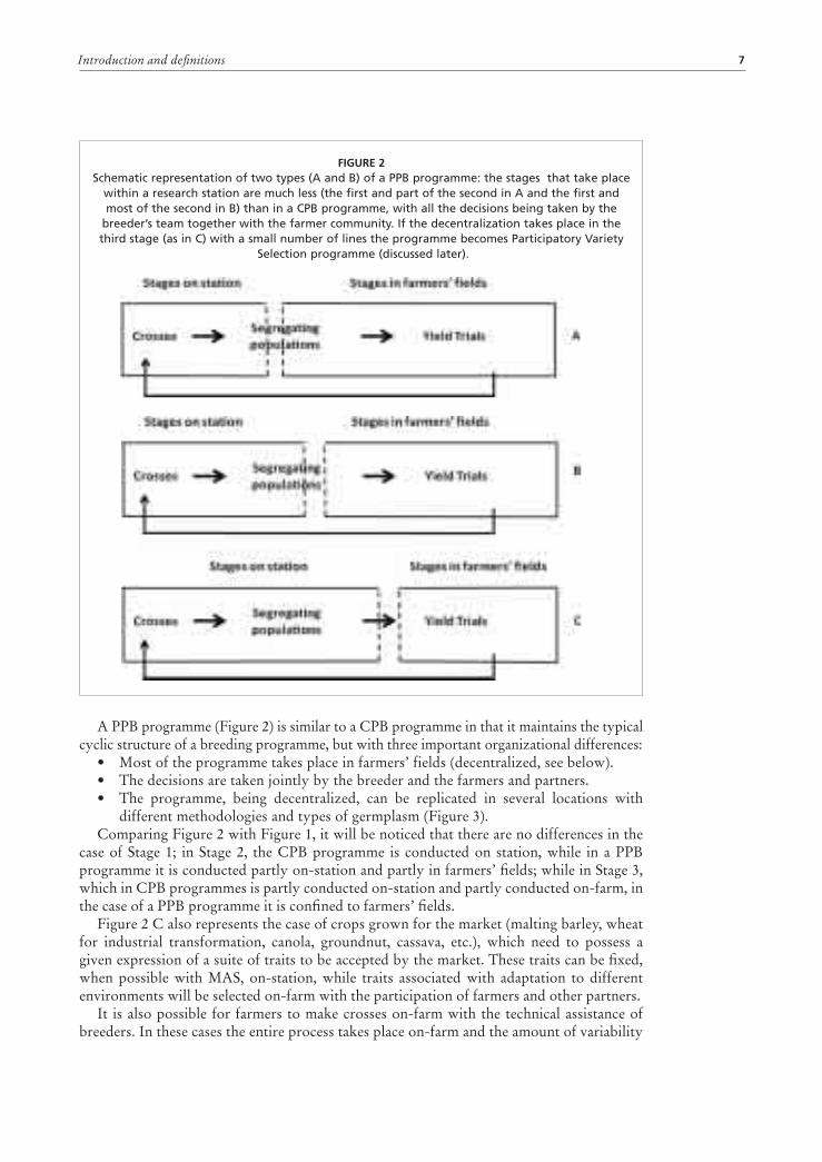
Introduction and definitions 7
A PPB programme (Figure 2) is similar to a CPB programme in that it maintains the typical cyclic structure of a breeding programme, but with three important organizational differences:
• Most of the programme takes place in farmers’ fields (decentralized, see below).• The decisions are taken jointly by the breeder and the farmers and partners.• The programme, being decentralized, can be replicated in several locations with
different methodologies and types of germplasm (Figure 3).Comparing Figure 2 with Figure 1, it will be noticed that there are no differences in the
case of Stage 1; in Stage 2, the CPB programme is conducted on station, while in a PPB programme it is conducted partly on-station and partly in farmers’ fields; while in Stage 3, which in CPB programmes is partly conducted on-station and partly conducted on-farm, in the case of a PPB programme it is confined to farmers’ fields.
Figure 2 C also represents the case of crops grown for the market (malting barley, wheat for industrial transformation, canola, groundnut, cassava, etc.), which need to possess a given expression of a suite of traits to be accepted by the market. These traits can be fixed, when possible with MAS, on-station, while traits associated with adaptation to different environments will be selected on-farm with the participation of farmers and other partners.
It is also possible for farmers to make crosses on-farm with the technical assistance of breeders. In these cases the entire process takes place on-farm and the amount of variability
FIGURE 2Schematic representation of two types (A and B) of a PPB programme: the stages that take place
within a research station are much less (the first and part of the second in A and the first and most of the second in B) than in a CPB programme, with all the decisions being taken by the
breeder’s team together with the farmer community. If the decentralization takes place in the third stage (as in C) with a small number of lines the programme becomes Participatory Variety
Selection programme (discussed later).
Plant breeding with farmers – a technical manual8
can be increased by crosses coming from the station. These cases are not very frequent as they require special skills and dedication.
The question is therefore of when during Stage 2 is the breeding material under selection—which is usually involves large numbers (up to several thousand lines)—taken into farmers fields. A general guideline is that the material can be reduced by conducting selection on-station for traits with high heritability (for example phenology) and for quality characters and disease resistance, but should not be submitted to selection for traits known to be affected by large G×E interactions. In a “mature” PPB programme, when farmer preferences are well identified, preliminary selection could be done on station, using MAS when appropriate, but only for those traits of importance to farmers and not affected by G×E interactions, hence with high heritability.
Under the section below on A General Model of Participatory Plant Breeding we will give some guidelines on when to transfer the breeding programme to the farmers’ fields, and with which type of breeding material.
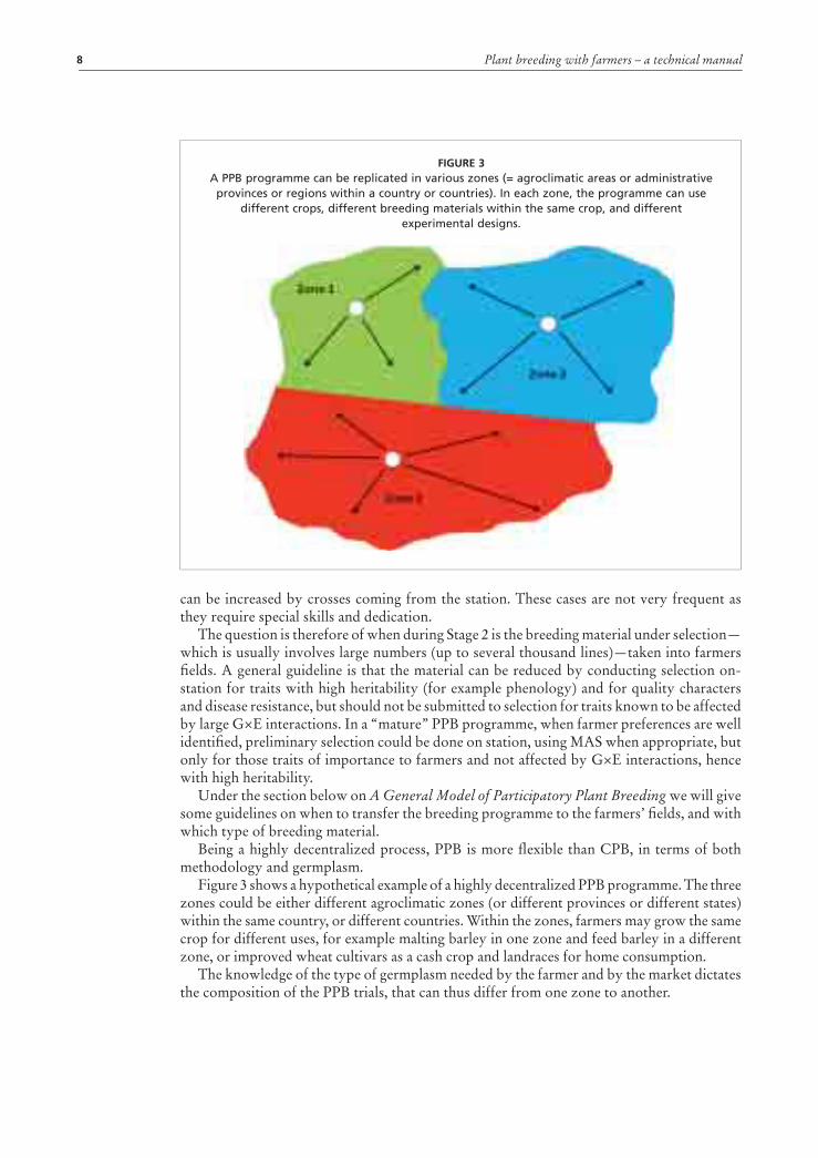
Being a highly decentralized process, PPB is more flexible than CPB, in terms of both methodology and germplasm.
Figure 3 shows a hypothetical example of a highly decentralized PPB programme. The three zones could be either different agroclimatic zones (or different provinces or different states) within the same country, or different countries. Within the zones, farmers may grow the same crop for different uses, for example malting barley in one zone and feed barley in a different zone, or improved wheat cultivars as a cash crop and landraces for home consumption.
The knowledge of the type of germplasm needed by the farmer and by the market dictates the composition of the PPB trials, that can thus differ from one zone to another.
FIGURE 3A PPB programme can be replicated in various zones (= agroclimatic areas or administrative provinces or regions within a country or countries). In each zone, the programme can use
different crops, different breeding materials within the same crop, and different experimental designs.

Introduction and definitions 9
PARTICIPATORY VARIETY SELECTION (PVS)Participatory Variety (or Varietal) Selection (PVS) is a process by which the field testing of finished or nearly finished varieties, usually only a limited number, is done with the participation of the partners. Therefore PVS is always an integral part of PPB, representing its final stages (Stage 4 in Figure 4), but can also stand alone in an otherwise non-participatory breeding programme if, using Figure 1 as an example, partners’ opinion is collected and used during the final stage, i.e. the on-farm trials.
Involvement of partners during the last stage of an otherwise non-participatory breeding programme has one major advantage and one major disadvantage: the advantage is that, if the partners’ opinion becomes part of the release process which follows the on-farm trials, only the variety(ies) that partners like will be proposed for release, thus increasing enormously the speed and the rate of adoption; the major disadvantage is that because partners’ opinion is sought at the very last stage of the breeding programme there may be nothing left among the varieties tested in the on-farm trials that meets partner expectations. This disadvantage may induce the breeder to seek partner participation at an earlier stage of the breeding programme, hence moving from PVS to PPB.
PVS may also be used as a starting point, a sort of exploratory trial, to help partners assessing properly the amount of commitment in land and time that a fully fledged PPB programme requires.
A GENERAL MODEL OF PARTICIPATORY PLANT BREEDINGA general model of PPB as defined above is shown in Figure 4. In this model, the first step (generation of genetic variability) is often, but not necessarily always, the responsibility of the research institution. It should be noted that when the genetic variability is created by making crosses, there is a substantial difference between making crosses, choosing the
FIGURE 4A general model of participatory plant breeding in which the research institute creates genetic variability, which is deployed in a number of farmers’ fields (four in this hypothetical example).
Plant breeding with farmers – a technical manual10
parents and designing the crosses. Making a cross is a purely technical operation, while choosing the parents and designing the crosses is a key decision in a breeding programme. In a breeding programme, a large part of the parental material used in crosses is represented by the best breeding material selected from the previous breeding cycle, and because in PPB the selection is done by both breeders and farmers, farmers do in fact participate in the choice of the parents to begin a new breeding cycle. Farmers may also explicitly choose parents by suggesting crosses to the research institution or learning to perform crosses themselves.
A number of stages of selection (four in this hypothetical example) are conducted in farmers’ fields with the participation of farmers and other stakeholders, with continuous interaction with the research institute (for example for the choice of appropriate experimental designs, data analysis, seed production, etc.) and with other farmers involved in the PPB programme. The selection is conducted independently in each location. This generally leads to the selection of different entries in different locations but does not exclude selecting the same material (see for example variety A being selected in locations 1 and 3 and variety B being selected in locations 2 and 3.
The best breeding material produced after the four stages of selection can be used by farmers as varieties and by the research institute as parental material for crosses to begin a new breeding cycle. It is important to notice that different locations may receive different types of germplasm of the same crop and select different varieties and that interaction among farmers may depend on their geographical location as well as communication technologies, language differences, etc.
In the case of self-pollinated crops and when the breeding method is the pedigree method, the selection in farmers fields can start with the segregating populations (for example, F2-derived F3 families) after their number is reduced by selection (including MAS) on station for disease resistance, for traits with high heritability (for example phenology), or for quality traits such as malting quality, or a combination. Distributing different segregating populations to different locations according to farmer preferences is an additional strategy to further reduce the amount of breeding material in any one farmer’s field. When the breeding programme uses the bulk-pedigree method, it is possible to start the field testing as early as the F3 bulks. In both cases, the yield testing should continue for at least four consecutive cropping seasons to generate sufficient information on the stability and performance of the breeding material for farmers to make a decision about adoption and for the variety release process.
In the case of population improvement of cross-pollinated crops, the recombination phase corresponds with the creation of genetic variability, which can be done on station while the selection and testing can be done in farmers’ fields. In the case of hybrid development, the creation and enrichment of breeding populations can be done—and in fact is being done, for example in China—in farmers’ field (Song et al.,2006). The production of uniform inbred lines to use as parents of hybrid cultivars can equally well be done on station or in farmers’ fields. In the latter case, because of the lower yield of inbred lines, a farmer compensation scheme should be envisaged. The advantage of developing inbreds in farmers’ fields is that selection during the inbreeding process is done in the real production environment, making sure that field heterogeneity does not bias the selection. Similarly in the case of test crosses, they can be more efficiently evaluated in farmers’ fields. While the actual production of the hybrid seed can be done both on station and in farmers’ field, the former has the advantage of not using farmers’ land and farmers’ labour. The field testing of the experimental hybrids has to be done for at least four cropping seasons, for the reasons given earlier. As in the case of self-pollinated crops, targeting germplasm to farmer preferences is an additional strategy to reduce the amount of breeding material under selection and testing at any one site.
In the case of vegetatively propagated crops after the initial crosses, all the subsequent generation are suitable for testing and selection in farmers’ fields. As in the case of the
Introduction and definitions 11
pedigree method for self-pollinated crops, the number of clones can be reduced on station by selecting for traits such as disease and or pest resistance, for traits with high heritability, and quality traits.
In Figure 4 the number of stages of selection has been set to four (defined as in most breeding programmes: Stage 1, Stage 2, Stage 3 and Stage 4) and it is envisaged that these stages are conducted in farmers’ fields with the participation of farmers and other stakeholders. The type of breeding material (segregating lines, bulks, clones, populations, hybrids) depends on the type of crop (self-pollinated, cross pollinated or vegetatively propagated) and on the breeding method. There is regular technical interaction with the research institute, for example, for the choice of appropriate experimental designs, data analysis, seed production, etc. The best breeding material produced after the four cycles of selection can be used by farmers as varieties, and by the research institute as parental material for crosses to begin a new breeding cycle. Other important features of the general model are summarized below.
• From Stage 1 to Stage 4 there is a progressive decrease in the amount of the breeding material (entries) and an increase in the amount of seed available for each entry. This, as we will see later, affects the choice of the experimental design and the number of locations where the entries are tested. It will be noticed that Stages 3 and 4 trials in this model are somewhat equivalent to the “mother” and “baby” trials concept (Snapp, 1999), respectively.
• The decision on what to promote from one stage to the next is taken by the farmers in ad hoc meetings held between harvesting and planting, and is based on both farmers’ visual selection during the cropping season and on the data collected by the researchers or by the farmers, or by both, after proper statistical analysis – as described later.
• In general, researchers have the primary responsibility for designing, planting and harvesting the trials, data collection and data analysis. Farmers are responsible for everything else and make all the agronomic management decisions. However, as the programme evolves, farmers can become responsible for planting, harvesting and data collection.
• Spatial analysis (Singh et al., 2003) of unreplicated or partially replicated or fully replicated trials and Genotype × Environment Interaction analysis by GGEbiplot (Yan, 2001) are used routinely for data analysis.
• In terms of the farmer’s time, the cost of participation ranges from two days to two weeks annually, depending on the level of participation.
• A back-up set of all the materials tested in Stages 1 to 4 is also planted at the research station to purify the bulks if pure lines are required in the case of self-pollinated crops, but, more importantly, to produce the seed needed for the trials and to insure against the risk of losing the trials to drought or other climatic events.
• In some countries, the farmers who are hosting trials are compensated (in kind) for the area used for the trials with an amount of seed equivalent to the production expected in an average year.
• Seed cleaning machinery is supplied to some villages to assist in the multiplication and dissemination of selected varieties following the fourth year of farmer selection.
• Screening for diseases and insect pests is carried out on-station before the first stage of yield testing on farmers’ fields to avoid the spreading of new diseases or pests, as PPB has been criticized (for example, in Syria) for the danger of spreading new diseases, yet interestingly in Syria, most of the wheat and barley varieties released through CPB are disease susceptible.
• The approach is flexible enough to accommodate biotechnological techniques, specifically Marker-Assisted Selection, after the first year of farmer selection (PPB

Plant breeding with farmers – a technical manual12
FIGURE 5Combinations of Centralization and Participation in breeding approaches.
should be able to provide reliable information on desirable traits that could later be evaluated via MAS should this be available and deemed desirable by farmers).
One of the consequences of a PPB programme is that the number of varieties it generates and the turnover of varieties are both higher than with CPB, thus increasing both spatial and temporal agro biodiversity. Also, it is not unusual that more varieties are adopted and cultivated within a region at any given time. While this is of course highly positive in terms of both agricultural biodiversity conservation and enhancement, and of protection against pests and diseases, it poses a number of challenges to seed production and for studies on the impact of PPB programmes (see page 115).
DECENTRALIZED PLANT BREEDINGDecentralization in the case of plant breeding is defined as selection and evaluation in the target environments, which are defined based on the repeatability of Genotype × Location interactions (see section on Genotype × Environment Interactions). Decentralized breeding does not necessarily mean selection for specific adaptation unless selection is conducted for superior performance in each target environment regardless of the mean performance.
Therefore, with reference to decentralization and participation, we can have the four combinations shown in Figure 5. While we have already discussed CPB, On-farm trials, PPB and PVS, Farmers’ selection on station deserves a comment.
Farmers’ selection on station, practiced as a form of PPB, cannot actually be considered as PPB because it does not create the same sense of ownership typical of a PPB programme. However, it is useful at the planning stage of a PPB programme to obtain information on farmer preferences which, because expressed in an environment that can be substantially different from a farmer’s field, are relevant only in the case of traits with high heritability.

13
How to get started: organizational issues
As defined earlier, a PPB programme is necessarily decentralized. We will therefore start by discussing the organizational issues involved in transforming a breeding programme from centralized to decentralized (Ceccarelli, 2009b).
Transferring a breeding programme to outside of a research station almost always implies losing some degree of control of a number of steps and operations. This is often associated with the perception that less control by scientists implies lower precision, and this explains the reluctance with which several plant breeders, particularly those in the developing countries, operate away from their research stations.
Within a research station, all the operations associated with running a breeding programme are shared by staff belonging to the same institution and having daily interaction (which does not necessarily make things easier). When a number of stages are transferred outside the research station, a number of operations can be, and actually should be, shared with staff belonging to other institutions or to out-posted staff of the same institution, or a combination of the two.
Depending on the presence or absence of a strong extension service, and reflecting the structure of the research institute responsible for the plant breeding, a number of different scenarios are possible.
In the case of countries with a strong extension service and the presence of regional (or sub-regional or provincial) research centres with infrastructure such as offices, computer facilities and agricultural equipment (including plot machinery), a PPB programme could be organized based on the following principles, which can be easily extended to international breeding programmes such as those of the Centers of the CGIAR.
• The scientist(s) at the institute’s headquarters are responsible for the preparations of trials (seed preparation, experimental design, and having the seed in envelopes ready for planting), the preparation of field books (or electronic files for electronic capture of field data), the preparation of draft field maps with possible alternatives for the layout of the trials, and the shipment of trials with all the detailed instructions for planting and note taking.
• At headquarters there will be a central database where all the information generated in the breeding programme is kept. Information generated in the regional centres should also be kept where it was generated, as a form of safety duplication.
• The main responsibility of the staff of the extension service is to collaborate in the selection of the sites and the specific fields, according to the type and objectives of trials and the general philosophy of the breeding programme.
• The research staff in the regional centres are responsible for implementing the trials on the ground, ensuring the required management, the timing of the field operations and eventually for collecting field data, which information is then transferred to headquarters for statistical analysis. Alternatively, when the necessary expertise is available, they can be requested to do the single-site statistical analysis, leaving responsibility for the multi-site statistical analysis to headquarters.
• Extension and research staff are also responsible for the organization of field days. These are useful not only to show the potential clients the new breeding material, but

Plant breeding with farmers – a technical manual14
also to understand through the interaction with farmers whether the experimental setting (location, type of soil, type of management, etc.) is actually representative of farmers’ conditions.
This overall organization is facilitated by involving all staff participating in the implementation of the breeding programme in regular meetings, through which the basic principles of the breeding programme are understood and shared by everyone. This obviously includes the full sharing of results among all the participants on an annual basis.
One important beneficial effect of this type of organization is that it replaces the traditional linear flow of information typical of agricultural research (Figure 6A) with a continuous exchange of information between the different partners (Figure 6B). As we will see below, this concept is fully developed in a PPB programme. In this type of scenario (Figure 6B), one of the main sources of additional cost associated with decentralized breeding, i.e. transportation and travel, is considerably reduced. In the case of countries where the extension service is limited or absent, all the responsibilities could be the responsibility of either research staff or NGOs.
In describing the organizational aspects of a decentralized breeding programme we are deliberately excluding the use of additional research stations as ‘decentralized’ sites, because, even if sub-stations capture differences in temperature and rainfall, they still suffer from all the management issues described earlier, and therefore they may not represent any real production environment. However, the regional stations can share with the headquarters station the responsibility for seed production.
A different scenario is that of those countries where, for various reasons, the national breeding programme cannot afford to go through the first stage of a breeding programme, i.e. the generation of genetic variability (regardless of the method), and therefore relies entirely on either locally collected germplasm, or on germplasm donated by breeding programmes in other countries or other research centres, such as international agricultural research centres (IARCs), or some combination. In such cases, the research station should be used for both seed multiplication and negative selection, particularly in the case of introduced germplasm, which might have photoperiod or vernalization requirements that makes it ill adapted to national conditions.
FIGURE 6PPB replaces the linear sequence Research >> Extension >> Farmers (A) with team work that
implies a continuous flow of information between the different partners (B). The Figure hypothesizes a general situation with a multitude of partners, some of whom may not be
present in specific situations. In B only some of the possible interactions are shown.

How to get started: organizational issues 15
Seed multiplication is necessary because the seed from germplasm collections and breeding material received from other programmes usually comes in very small quantities. The steps following the initial seed multiplication depend on the breeding methods and on the type of genetic material received or collected, but will vary from a centralized, on-station, programme of selection, evaluation and testing, with only the final stages transferred to farmers fields, through to a decentralized non participatory programme or to a PPB programme.
At the beginning of the manual we defined PPB programmes as breeding programmes in which selection and testing are conducted in the target environment(s) with the participation of the users. Here we will add that, in order to reach its maximum effectiveness, the participation of users should take place as early as possible, and ideally at the beginning of Stage 2 in a plant breeding programme, as described in Figure 1. For traits that are not affected by G×E interaction (see page 86) it may also be desirable to involve farmers in the choice of parents on station, or to plant a set of parents on farm and involve the farmers in the choice of the most desirable parents.
The organizational aspects of a PPB programme do not differ conceptually from those of a CPB programme. The major difference is that the decisions and the choices for the organizational aspects involve all the stakeholders, and the type of participation depends on how, when and which stakeholders are involved.
We will examine the following organizational aspects:• Setting criteria to identify target environments and target users.• Choice of the target environment and users.• Type of participation.• Choice of genetic material.• Choice of parental material.• Choice of breeding method.• When farmer participation should start.• Naming of varieties.• Management of trials in farmers’ fields.• Managing equipment.• Farmer selection.• Visits to farmers.• Managing the transition phase.• Sharing and disseminating findings.One fundamental issue in discussing organizational issues with farmers’ communities
is to pose and justify the problem, rather than simply presenting a solution. The solution should come from the community, and if the community or the individual farmers are not prepared to solve the problem, a possible solution can be offered, but only as a suggestion.
SETTING CRITERIA TO IDENTIFY TARGET ENVIRONMENTS AND TARGET USERS A PPB programme may lose a great deal of its potential effectiveness if the sample of both environments and users in which the programme is implemented does not represent both the target environments and the target users. In order to do that, setting the criteria for identification of the target environments and users is a critically important step.
In setting the criteria, it is useful also to assign priorities to the different categories of environments and users so that, depending on the resources available to the programme, environments and users can be added or discontinued on the basis of priorities established in an ideal context.
The most obvious criterion for the choice of the target physical environments, is the representativeness of the major production areas for a given crop (or for the crops covered by the programme) in terms of climatic conditions (temperature, rainfall, elevation), agronomic
Plant breeding with farmers – a technical manual16
practices, soil types, landscape, etc. The criteria for the choice of the socio-economic environments are closely interconnected with those of the target users. The programme has therefore to decide whether to work for all the various socio-economic environments present in the target area, or to privilege the most difficult environments where farmers have fewer opportunities for market access and where most of the agricultural products are used within the farms or within the community, or to work only for the most favourable, high potential, environments possibly market oriented. As mentioned earlier, PPB has evolved mainly to address the difficulties of poor farmers in developing countries (Ashby and Lilja, 2004), which have been largely bypassed by the products of CPB. In fact there is no reason why the approach should be confined to working only with low-income farmers. Basically, when done properly, PPB is an approach that, even if applied in a variety of modes, merges the technical knowledge of the ‘scientists’ with the knowledge of the ‘farmers’, which is historically based on millennia spent in domesticating wild plants and adapting the resulting crops to a multitude of different environments and uses. Therefore, in principle, PPB can apply equally well even in situations of market-oriented agriculture in favourable environments. It seems particularly suited for organic and bio dynamic agriculture, and in developed countries, interest in PPB programmes is primarily coming from organic farmers (Lammerts van Bueren and Myers, in press).
The main criteria for identifying farmers can be grouped in three broad categories:• Farmer characteristics. These include language, religion, ethnicity, caste, age,
gender, income, education, market relations or orientation, membership in farmer organizations (unions or cooperatives), and relationships among groups within the same community and between communities.
• Farmer expertise. This includes the need to understand whether farmers are already practicing some types of plant improvement, as this is essential in the choice of the breeding methodology (see below). In some communities, e.g. Eritrea, specific individuals have specific responsibilities in relation to crop and variety introduction (Soleri et al., 2002).
• Farmer needs. These include the needs of different groups, their perception of risk and hence the type of variety they consider most appropriate in term of stability and yield (Anderson, 1974; Soleri et al., 2002), and the need for special quality attributes for either feed or food, or both. These include also the farmers’ understanding of production limitations with reference to the use of fertilizers, appropriate rotations and irrigation. It is also important to understand farmers’ needs in terms of seed supply, because it makes a large difference whether the farmers predominantly use their own seed (or the seed of their neighbours), or usually buy seed from the formal sector.
In these meetings it is also essential to understand what sources of seed farmers use for various crops, to anticipate which type of change the participatory programme might introduce, and to make sure that farmers are aware and prepared to absorb these changes.
CHOICE OF THE TARGET ENVIRONMENT AND USERSOnce the criteria are set, the actual choice of locations and users requires the involvement of partners who have very good knowledge of both the environment and the users. These are typically the staff of the extension service or the staff of the provincial research stations. The first step is to set meetings with all the stakeholders with the objective of identifying partners and locations.
In this phase there are some potential biases that can affect the success of PPB. Key decisions affecting the participatory programme are (i) whether to seek individual or group participation; (ii) whether the participants should be experts (germplasm experts are farmers

How to get started: organizational issues 17
who regularly experiment with varieties, are able to recognize important intra- as well as inter-varietal differences, and who target specific varieties to different micro-niches) or whether they should represent the wider community; and (iii) whether equity should be the main objective in the identification of the users. Meetings with all different types of farmers together may be inappropriate without a proper knowledge of the power relationships within the community. This usually leads to a few farmers monopolizing all the discussions, reducing the possibilities for others to express their views. This danger varies greatly with the culture: in some cultures, women are not even allowed to attend meetings; in others, they can participate with a passive role; and in others they can participate freely and with the same rights as the men. Therefore, it is not possible to give a ‘cookbook formula’ for what works better. In general, if some groups or individuals tend to be discriminated against, it may be appropriate to have separate meetings with different social, gender, age or wealth groups.
In the process of choice of users, it is very important to clarify (i) what plant breeding can offer and how long it can take; (ii) what sort of commitment in land, time and labour is required from the farmer; (iii) what are the risks for the farmer and how these can be compensated for (in-kind compensation vs money); and (iv) what overall benefits farmers can expect if everything goes well.
The choice of sites is both at the macro-level (choice of villages or locations within a country or a region) and at the micro-level (choice of the field within a village for planting the trial(s)).
The choice of the sites at the macro-level is associated with the issue of the breeding philosophy: whether these sites should be sufficiently representative to allow some degree of extrapolation of the results to other sites, or whether the priority should be to meet farmers’ needs within micro-environments. In practice, it is advisable that sites must represent the range of environmental and agronomic conditions in which the crop is grown, because this is known to have a major effect on farmers’ selection (Ceccarelli et al., 2000, 2003).
An “ideal” test environment should be both discriminating of the genotypes, repeatable over years and representative of the target environment (Yan et al., 2011). The “Discrimination vs Representativeness” of test sites will be discussed later in the section on GGEbiplot software (see page 90).
PPB programmes are often seen exclusively as programmes leading to niche varieties, adapted to only a restricted complex of environmental and social characteristics. This is not necessarily true, as the type of adaptation (narrow or wide) of the varieties emerging from a PPB programme is largely dependent upon the nature of the locations and the users. If the locations covered by the programme represent a mix of favourable and unfavourable growing conditions, it could be expected that the more uniform environmental conditions that generally characterize favourable environments will led to the selection of the same varieties across a number of locations (widely adapted in a geographical sense), assuming that farmers’ preferences are also homogenous across the same locations. In less favourable conditions, one can expect that more location-specific varieties (narrowly adapted) will be selected. Eventually, even if the selection is conducted independently in each of many locations, giving the impression that selection is for specific adaptation, the process will not discard a truly widely adapted genotype if such a genotype does exist in the breeding material (Ceccarelli, 1989). Therefore a PPB programme easily results in a mixture of widely and narrowly adapted varieties.
What is discussed above also depends on the definition of wide and narrow adaptation. Narrow and wide are relative terms; therefore, for international breeding programmes and for seed companies, a widely adapted variety is a variety performing well in a number of countries, while for national breeding programmes it is a variety performing well in several locations within a country, while, ultimately, to farmers is a variety performing well across

Plant breeding with farmers – a technical manual18
cropping seasons (stable over time) – without too much concern whether it performs well elsewhere (stable over space).
The participation of farmers in the choice of the fields is unavoidable because it is associated with the relevance of the results and with the issues of ‘who participates’ and ‘who benefits’: it is at this point that small-scale farmers run the risk of being excluded as active participants because their land is not large enough to host trials in addition to their subsistence crops. As we will see later, it is possible to find experimental designs that allow the distribution of a relatively large number of entries in small blocks, each planted in a different farmer’s field. It is difficult to reach an optimal allocation of resources regarding the number of sites and the number of farmers at each site. As we will see later, it is possible to organize a PPB programme in such a way that G×E interaction, and more specifically Genotype × Location (G×L) and Genotype × Years within Locations (G×Y(L)) will eventually optimize the overall structure, at least from a biological point of view.
TYPE OF PARTICIPATIONSeveral scientists (Biggs and Farrington, 1991; Pretty 1994; Lilja and Ashby 1999a, b; Ashby and Lilja, 2004; McGuire, Manicad and Sperling, 1999; Weltzien et al., 2000, 2003; Ashby, 2009) discriminate among different types or modes of participation, which are not necessarily mutually exclusive, although there may be trade-offs among the impacts of the different types. We will not discuss these different typologies because field experience indicates that PPB is a continuously evolving process. It is quite common that, as farmers become progressively more empowered—an almost inevitable consequence of a truly PPB programme—the type or mode of participation also evolves.
CHOICE OF GENETIC MATERIALThe type of genetic material to be used in the programme needs to be discussed with the farmers. Initially, the scientists may find that farmers are not aware of the diversity within the crop, and in this case our suggestion is to start with a wide array of genotypes representing as wide range of diversity as possible. But there are cases where farmers have previous experience with various type of germplasm and they may feel very strongly concerning one or more types of specific germplasm type. For example, in Syria, farmers grow two barley landraces: one with black seed, which is grown predominantly in dry areas, and one with white seed, which is grown predominantly in wetter areas. Farmers feel very strongly about the seed colour and therefore in the participatory barley breeding programme in Syria we make available different initial genetic material in the two areas. Similarly in Syria, there is a strong preference for two-row barleys, with very few exceptions, while in North Africa there is a strong preference for six-row types. The issue of the type of genetic material also includes the issue of the checks. As we will see later in the section on experimental designs, the checks have the dual purpose of providing an estimate of error variance (for example, in unreplicated trials with systematic checks) and to provide a comparison for farmers during selection. The ideal solution is to have a well adapted variety that fits both purposes, and if the choice of the check(s) is left, as it should be, to the farmers, they usually choose a variety that is suitable for both.
CHOICE OF PARENTAL MATERIALThe choice of parental material is of critical importance in a breeding programme and it depends largely on the number of target environments and objectives (Witcombe and Virk, 2009). Therefore the crossing-block—this is usually the term used for the set of parental material used in the crossing programme—is usually very large (300–400 lines and varieties) in an international breeding programme, such as those of the International Agricultural
How to get started: organizational issues 19
Research Centres (IARCs), that have multiple objectives and address a large population of target environments. Here we only add that, as in a CPB, the parental material in a PPB programme is, with few exceptions, the best material selected by farmers in the previous cycle.
CHOICE OF BREEDING METHODThe breeding method is only one of the factors determining the success of a breeding programme; others include the identification of objectives and the choice of suitable germplasm (Schnell, 1982).
In CPB, the choice of the breeding method is purely the responsibility of the breeder and is largely influenced by the breeder’s scientific background and by the mandate of the organization, public or private, for which the breeder works.
In PPB, the choice of the breeding methods cannot be made without considering whether and how farmers are handling genetic diversity. The rationale is as follows. As shown in Figure 1, the generation of variability is the first step of any breeding programme, conventional or participatory, followed by the utilization of variability and eventually the testing of the prospective varieties. In a number of countries, farmers do use genetic diversity either as a specialized activity within the community, or as an individual initiative. For example, in Eritrea it is common for farmers to select individual heads within a wheat or a barley plot, plant them as head rows in a small portion of their field, decide whether to bulk one or more rows and start testing the bulk in the field of other farmers, initially on a small scale and gradually on a larger area. One of the most widely grown wheat varieties in the country has been developed starting from a small seed sample bought by an expert farmer in a local seed market and planted initially as spaced plants. In Nepal, before harvesting the crop, a woman farmer growing an old barley landrace habitually collects a sample of heads representing all the different morphological types present in the field to produce the seed to be planted in the following cropping season. In the northernmost part of India (Sikkim) farmers maintain and improve their rice varieties by carefully selecting (before harvesting) the best panicles, which are then stored for the next planting season, while the rest of the crop is consumed (Ceccarelli, 2011). In contrast, in Syria and in many other countries in the Near East and North Africa, the selection unit is a plot, and excessive heterogeneity within a plot not only is not exploited, but is also considered undesirable.
These examples indicate that, even within the same crop, a PPB programme may have to use different breeding methods, at least at the beginning of the programme, to ensure full participation. It is obvious that a blanket approach, based on the same breeding method used everywhere regardless of whether and which skills farmers have in handling genetic variation, cannot ensure true participation, as farmers will be confronted with methodologies they cannot relate to anything they are familiar with.
In addition to the examples given earlier, breeding methods may differ for the same crop within the same country. Using Africa as an example, barley is grown in Ethiopia and Eritrea both as food and feed (largely landraces) and also for malt production for local breweries. While population methods can well be used in the first case, pedigree breeding or SSD is more suitable in the second.
An issue related to the choice of the breeding method is how much breeding material farmers can handle. This is a controversial issue, and many scientists believe that farmers can only handle a very limited number of genotypes and therefore, implicitly, believe that the only form of possible participation is PVS. If true, this will make it impossible to implement true PPB programmes, because plant breeding needs to start from a sufficiently large sample of genetically variable material.
Field experience shows that when deciding on the number of genotypes farmers can handle, it is very dangerous to make assumptions before discussing the issue with them.
Plant breeding with farmers – a technical manual20
The choice of the breeding method also depends on the desired genetic structure of the final product, i.e. pure lines, mixtures, hybrids or open pollinated varieties. It is important to note that farmers can change the type of final product originally planned by the breeder. For example, in Syria, where, in the case of self-pollinated crops, the formal system only accepts pure lines for release, farmers do not mind adopting bulks as long as they are not too phenotypically heterogeneous. In the case of barley, we also have the example of one farmer testing the advantages of a mixture of a 6-row genotype, adapted to high rainfall and resistant to lodging, with a 2-row genotype adapted to low rainfall and susceptible to lodging. Similarly in Egypt, we found that farmers plant a mixture of all the lines selected one year earlier (Grando, pers. comm.). A similar observation has been made in Iran, where the use of mixtures by the farmers involved in a PPB programme is increasing.
In principle, all breeding methods used in CPB can be employed in PPB, keeping in mind that ‘participatory’ does not mean that ALL the breeding material must ALWAYS be planted in farmers’ fields.
Several examples of different breeding methods used in actual participatory breeding programmes can be found in Almekinders and Hardon (2006).
WHEN FARMER PARTICIPATION SHOULD STARTGiven that plant breeding is a cyclic process, one organizational issue that is often debated is the stage of the plant breeding programme at which participation should start. As mentioned earlier, this issue in effect makes the difference between PPB and PVS, as in PVS farmer participation takes place during the third stage of the breeding process, after the genetic variability available at the beginning of the cycle has—usually—been drastically reduced. We believe that farmer participation should, at a minimum, coincide with the second stage of a breeding programme, when the genetic variability is still at or near its maximum. There are examples of PPB programmes where farmers can start as early as making crosses, such as the participatory rice breeding programmes in Bhutan, the Philippines and Viet Nam (SEARICE, 2003; Pelegrina et al., 2006), which does not necessarily imply only emasculation and manual pollination, but, for example, mixing different genotypes or cultivars of cross-pollinated crops to facilitate inter-crossing. A similar example is the improvement of maize landraces coordinated by the Centre for Chinese Agricultural Policy (CCAP), a leading agricultural policy research institution that is part of the Chinese Academy of Sciences (CAS) (Song et al., 2006). Even when farmers do not manually make the crosses, in a PPB programme that runs over cycles of selection and recombination like any other plant breeding programme, farmers control the crossing programme by selecting the best entries, which are usually the parents of the following cycle, as discussed earlier under choice of parental material.
Eventually, a breeder planning to start a PPB programme is faced with the issue of whether the breeding method used in a non-participatory programme needs to be changed. While there are breeding methods that are easier to fit into a participatory context, a breeder does not have to necessarily change the breeding method, given what was said earlier about fitting the method to whatever type of breeding farmers are already doing. Here we might add that, like other aspects of PPB, the methodology can also evolve as new farmer skills emerge. Several examples can be found in Almekinders and Hardon (2006).
NAMING OF VARIETIESAt the end of each cycle of the programme, if the cycle has been successful in producing a potential new variety, one issue is how to identify the variety. Given that the numbers or pedigrees used by the breeders can be meaningless to the farmers, and that several farmers may have contributed to select the new variety, the naming process should be undertaken with the community. In mature PPB programmes it is now a common procedure for farmers
How to get started: organizational issues 21
to name those lines that they decide to plant on large areas after the 4th stage of yield trials. In mature programmes this rarely results in conflict and the names chosen range from the name of village, the name of the son or daughter of a leading farmer, or symbolic names such as peace, unity, etc. In relatively young programmes we found, surprisingly, that the choice of the name may also be a moment of conflict the first time it occurs, and that therefore it may be wise to raise the issue some time before a variety is developed, or even at the beginning of the programme.
Naming of varieties has an important effect in creating a sense of ownership, and has also legal implications if PPB varieties are officially released.
MANAGEMENT OF TRIALS IN FARMERS’ FIELDSThe organizational issues of implementing trials in farmers’ fields differ considerably from those in a research station.
The first differences are issues such as the choice of the actual portion of land on which to plant the trial, the total number of plots in each trial, the type of controls (check varieties), the plot size, the seeding rate, the distance between rows, the dates of planting and harvesting, the importance of border (guard) rows and plots: all these have to be discussed with each community in each location. It is not simply a matter of courtesy. Farmers’ interest in the trial is directly proportional to their participation in its design and management. The inability of the scientists to accommodate farmers’ requirements may lead to a total lack of interest by the farmers. For example, in the case of barley in Syria, farmers believe that seeding rate is extremely important. Whether this belief is correct or not is immaterial, because if the scientists ignore farmers’ practices and use the seeding rate they believe right, farmers may even refuse to carry out selection. Therefore, in the PPB programme in Syria for example, we are using as many as eight different seed rates, ranging from 100 kg/ha to 250 kg/ha. As this is believed by the farmers to have a major effect on barley yields, an important side-activity would be to organize visits by farmers to locations where a different seed rate is used; this might be the best way to generate an interest in testing alternative seeding rates.
The choice of land, which in a conventional breeding programme usually depends on the farm manager, in the case of PPB has to be agreed on by the farmer. It has to represent a suitable rotation and have good uniformity (this should be checked the year before, together with the past history of the field). The size required by the trial may be smaller than that allocated by the farmer to that specific rotation. In this case, the extra land has to be planted by the scientists using a variety of the same crop chosen by the farmer.
MANAGING EQUIPMENTManaging the equipment in a PPB programme can be a challenging issue. If the country has a network of research stations each with its own equipment, it is obviously more economical that each station uses its own equipment for all the field operations. Where machinery has to be moved from one central research station to all the trials sites, the number of sites and of trials has to be adjusted to allow all the necessary operations to be performed in time. Usually farmers are extremely concerned about planting and harvesting at the right time, and if the choice is between having several locations and being late in both planting and harvesting some of them, it is advisable to reduce them to a number that can be managed properly. The issue of timely harvesting, in the case of completely mechanized crops, can be solved by estimating yield through a hand-harvested sample of the plots. This has the additional advantage of estimating the total biological yield, a character of major importance to farmers in many developing countries. The farmers can then combine-harvest whatever is left in the field (some farmers have actually used the seed obtained by harvesting the leftovers – a complex mixture – for planting and have achieved very large yields). This of course assumes that the seed requirements for the following year are satisfied by the seed
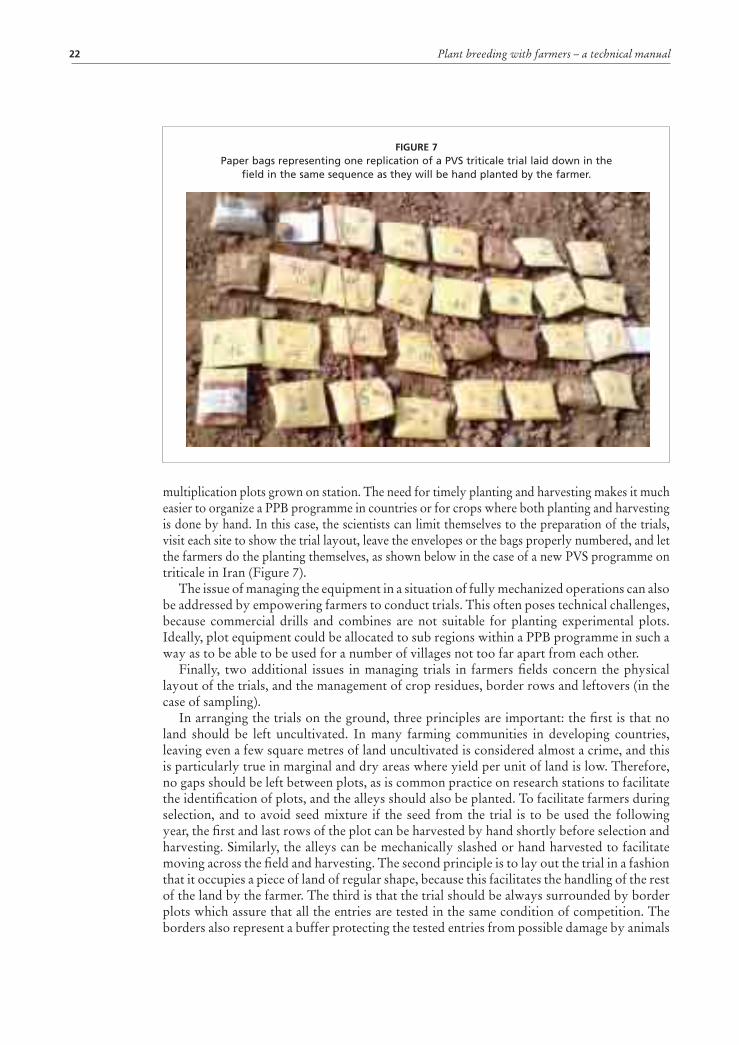
Plant breeding with farmers – a technical manual22
multiplication plots grown on station. The need for timely planting and harvesting makes it much easier to organize a PPB programme in countries or for crops where both planting and harvesting is done by hand. In this case, the scientists can limit themselves to the preparation of the trials, visit each site to show the trial layout, leave the envelopes or the bags properly numbered, and let the farmers do the planting themselves, as shown below in the case of a new PVS programme on triticale in Iran (Figure 7).
The issue of managing the equipment in a situation of fully mechanized operations can also be addressed by empowering farmers to conduct trials. This often poses technical challenges, because commercial drills and combines are not suitable for planting experimental plots. Ideally, plot equipment could be allocated to sub regions within a PPB programme in such a way as to be able to be used for a number of villages not too far apart from each other.
Finally, two additional issues in managing trials in farmers fields concern the physical layout of the trials, and the management of crop residues, border rows and leftovers (in the case of sampling).
In arranging the trials on the ground, three principles are important: the first is that no land should be left uncultivated. In many farming communities in developing countries, leaving even a few square metres of land uncultivated is considered almost a crime, and this is particularly true in marginal and dry areas where yield per unit of land is low. Therefore, no gaps should be left between plots, as is common practice on research stations to facilitate the identification of plots, and the alleys should also be planted. To facilitate farmers during selection, and to avoid seed mixture if the seed from the trial is to be used the following year, the first and last rows of the plot can be harvested by hand shortly before selection and harvesting. Similarly, the alleys can be mechanically slashed or hand harvested to facilitate moving across the field and harvesting. The second principle is to lay out the trial in a fashion that it occupies a piece of land of regular shape, because this facilitates the handling of the rest of the land by the farmer. The third is that the trial should be always surrounded by border plots which assure that all the entries are tested in the same condition of competition. The borders also represent a buffer protecting the tested entries from possible damage by animals
FIGURE 7Paper bags representing one replication of a PVS triticale trial laid down in the
field in the same sequence as they will be hand planted by the farmer.

How to get started: organizational issues 23
or humans, and may offer the opportunity to multiply the seed of a variety needed by the farmers.
The management of trials residues (borders, fillers around trials, border rows and what is left of a plot after taking samples) is an important organizational issue because it is a potential source of dispute. As a general principle, as in many other organizational issues in PPB, this needs to be discussed in advance with farmers, justifying why the handling of experimental plots is different from the handling of a field planted for large-scale production, underlining the need to generate information to use later in selection, and the need for as much precision and accuracy as possible to obtain correct estimates of the genotypic values of the breeding material (the scientists do not necessarily have to use these terms when discussing with farmers!). As mentioned earlier, the guiding principle is to justify and pose the problem, and involve farmers in the process of finding the most mutually suitable solution.
FARMER SELECTIONA key organizational issue in PPB is the selection done by the farmers. This is one of the most important operations (and one that makes the breeding programme participatory). It is also one of the activities that, if done properly, can generate a strong sense of ownership, and enhance farmer skills as far as the knowledge of the genetic material is concerned.
As for other organizational issues, it is impossible to give general recommendations, because the baseline can be very different in different communities. One of the extreme situations is represented by communities where there is only a vague notion that different varieties do exist, but farmers have had only sporadic contacts with scientists, and these contacts have been mostly of the type “I am here to tell you what to do; you do it, and I will come back to check if you did it well!”. In these communities, farmers often do not know about the sexual reproduction process in plants and therefore the diversity itself within a crop is surrounded by an aura of mystery. The other extreme is represented by communities who already have a solid experience in breeding and experimenting.
Most of our experience has been with the first type of situation, which is not necessarily the most difficult, but is certainly one in which PPB takes more time to develop. Therefore we will illustrate some general principles that we followed with the first type of situation, and how these principles need to be modified in the case of the second situation. We will consider in particular two aspects of farmer selection, namely ‘when to select’ and ‘how to select’. The question is often asked whether the maximum number of lines to select should be set in advance. We believe that this should be left open within the limits imposed by the experimental design to be used in the following season, as explained below under experimental designs.
The timing of selection depends strongly on the crop and its uses, on the environment and on the traits farmers consider important. This is a typical aspect of the overall activity, and one which needs to be discussed with farmers during the planning of the programme because it has implications for the amount of time farmers need to allocate to selection and on the total number of experimental units (plots or plants) farmers can handle. It also has implications for the degree of involvement of the scientists where some of the traits that are important to the farmers need to be measured.
The choice of the ideal time for selection is highly individual: some farmers prefer to visit the field often during the cropping season, while others, particularly in unpredictable environments, claim that only shortly before harvesting is it possible to assess the real value of the breeding material. Farmers may also change their preferences in relation to both when and how to select. Farmers who were used to an organized ‘selection day’, whereby all the farmers assembled at a meeting point and visited and scored the various trials, subsequently demanded to do the selection by themselves on a date convenient to them. In fact, it is
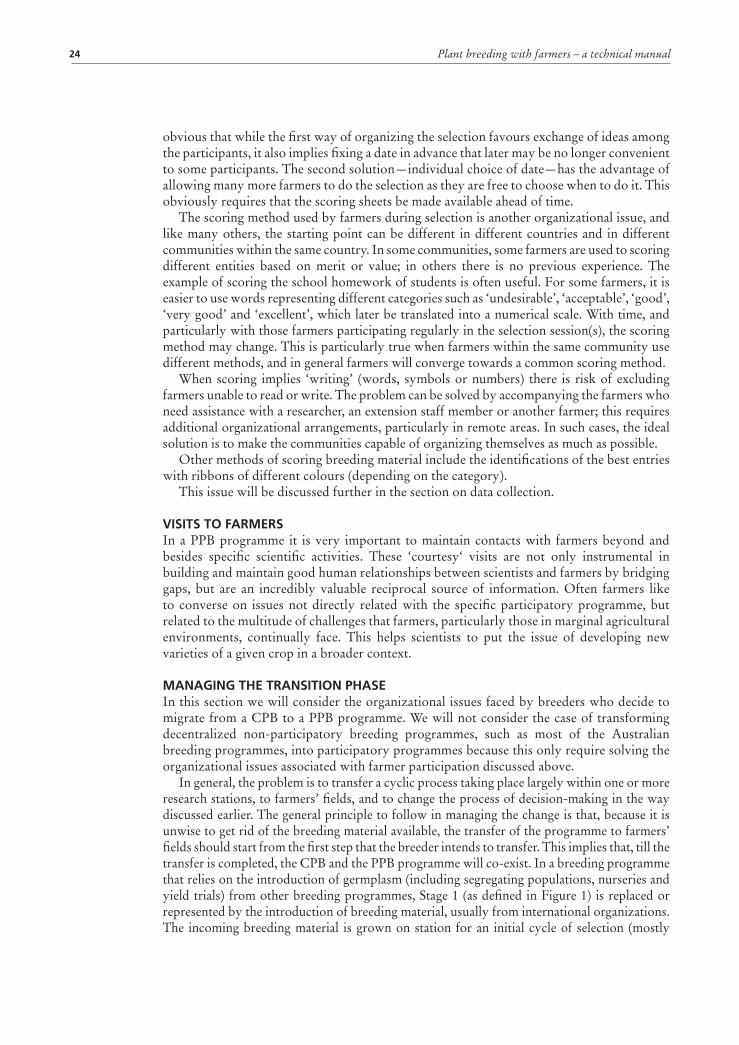
Plant breeding with farmers – a technical manual24
obvious that while the first way of organizing the selection favours exchange of ideas among the participants, it also implies fixing a date in advance that later may be no longer convenient to some participants. The second solution—individual choice of date—has the advantage of allowing many more farmers to do the selection as they are free to choose when to do it. This obviously requires that the scoring sheets be made available ahead of time.
The scoring method used by farmers during selection is another organizational issue, and like many others, the starting point can be different in different countries and in different communities within the same country. In some communities, some farmers are used to scoring different entities based on merit or value; in others there is no previous experience. The example of scoring the school homework of students is often useful. For some farmers, it is easier to use words representing different categories such as ‘undesirable’, ‘acceptable’, ‘good’, ‘very good’ and ‘excellent’, which later be translated into a numerical scale. With time, and particularly with those farmers participating regularly in the selection session(s), the scoring method may change. This is particularly true when farmers within the same community use different methods, and in general farmers will converge towards a common scoring method.
When scoring implies ‘writing’ (words, symbols or numbers) there is risk of excluding farmers unable to read or write. The problem can be solved by accompanying the farmers who need assistance with a researcher, an extension staff member or another farmer; this requires additional organizational arrangements, particularly in remote areas. In such cases, the ideal solution is to make the communities capable of organizing themselves as much as possible.
Other methods of scoring breeding material include the identifications of the best entries with ribbons of different colours (depending on the category).
This issue will be discussed further in the section on data collection.
VISITS TO FARMERSIn a PPB programme it is very important to maintain contacts with farmers beyond and besides specific scientific activities. These ‘courtesy‘ visits are not only instrumental in building and maintain good human relationships between scientists and farmers by bridging gaps, but are an incredibly valuable reciprocal source of information. Often farmers like to converse on issues not directly related with the specific participatory programme, but related to the multitude of challenges that farmers, particularly those in marginal agricultural environments, continually face. This helps scientists to put the issue of developing new varieties of a given crop in a broader context.
MANAGING THE TRANSITION PHASEIn this section we will consider the organizational issues faced by breeders who decide to migrate from a CPB to a PPB programme. We will not consider the case of transforming decentralized non-participatory breeding programmes, such as most of the Australian breeding programmes, into participatory programmes because this only require solving the organizational issues associated with farmer participation discussed above.
In general, the problem is to transfer a cyclic process taking place largely within one or more research stations, to farmers’ fields, and to change the process of decision-making in the way discussed earlier. The general principle to follow in managing the change is that, because it is unwise to get rid of the breeding material available, the transfer of the programme to farmers’ fields should start from the first step that the breeder intends to transfer. This implies that, till the transfer is completed, the CPB and the PPB programme will co-exist. In a breeding programme that relies on the introduction of germplasm (including segregating populations, nurseries and yield trials) from other breeding programmes, Stage 1 (as defined in Figure 1) is replaced or represented by the introduction of breeding material, usually from international organizations. The incoming breeding material is grown on station for an initial cycle of selection (mostly
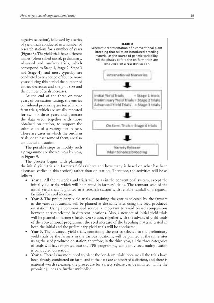
How to get started: organizational issues 25
negative selection), followed by a series of yield trials conducted in a number of research stations for a number of years (Figure 8). The yield trials have different names (often called initial, preliminary, advanced and on-farm trials, which correspond to Stage 1, Stage 2, Stage 3 and Stage 4), and most typically are conducted over a period of four or more years: during this period the number of entries decreases and the plot size and the number of trials increases.
At the end of the three or more years of on-station testing, the entries considered promising are tested in on-farm trials, which are usually repeated for two or three years and generate the data used, together with those obtained on station, to support the submission of a variety for release. There are cases in which the on-farm trials, or at least some of them, are also conducted on station.
The possible steps to modify such a programme are shown, year by year, in Figure 9.
The process begins with planting the initial yield trials in farmer’s fields (where and how many is based on what has been discussed earlier in this section) rather than on station. Therefore, the activities will be as follows:
• Year 1. All the nurseries and trials will be as in the conventional system, except the initial yield trials, which will be planted in farmers’ fields. The remnant seed of the initial yield trials is planted in a research station with reliable rainfall or irrigation facilities for seed increase.
• Year 2. The preliminary yield trials, containing the entries selected by the farmers in the various locations, will be planted at the same sites using the seed produced on station. Using a common seed source is important to avoid biased comparisons between entries selected in different locations. Also, a new set of initial yield trials will be planted in farmer’s fields. On station, together with the advanced yield trials of the conventional programme, the seed increase of the breeding material tested in both the initial and the preliminary yield trials will be conducted.
• Year 3. The advanced yield trials, containing the entries selected in the preliminary yield trials by the farmers in the various locations, will be planted at the same sites using the seed produced on station; therefore, in the third year, all the three categories of trials will have migrated into the PPB programme, while only seed multiplication is conducted on station.
• Year 4. There is no more need to plant the ‘on-farm trials’ because all the trials have been already conducted on farm, and if the data are considered sufficient, and there is material worth releasing, the procedure for variety release can be initiated, while the promising lines are further multiplied.
FIGURE 8Schematic representation of a conventional plant
breeding that relies on introduced breeding material as the source of genetic variability. All the phases before the on-farm trials are
conducted on a research station.
Plant breeding with farmers – a technical manual26
SHARING AND DISSEMINATING FINDINGS Once the results of the PPB trials for each location have been compiled, they should be shared with all the stakeholders (other farming communities, NGOs and the extension service). This can be done through a combination of methods, including:
• organizing a field day at which participating farmers explain and present their work and results;
• documenting the work using radio and television;• holding stakeholder meetings to share the results;• training participating farmer groups; and• producing descriptive sheets for each farmer’s selected variety.
FIGURE 9Steps to modify a conventional plant breeding programme that relies on introduced breeding
material as the source of genetic variability, into a decentralized-participatory breeding programme. In each box the conventional programme is on the left and the participatory
on the right.

27
Data collection
The trials conducted in a PPB programme need to generate the same quantity of information and of superior quality (due to being enriched by farmer and end user feedback from an early stage) as in a CPB programme, for two reasons: first, because the information has to be used to decide which material to promote and which material to discard, the scientists have a moral obligation to provide farmers with the most precise data possible, and, second, because the information can be later used when submitting a variety for release. We learned that in addition to the visual selection, farmers may want to have access to some quantitative data to reach a final decision. This is an additional issue to discuss at the onset of the programme because if this is required by the farmers, the trials have to be organized in such a way as to allow data to be collected on the traits considered important by farmers, the results to be analysed with appropriate statistical methods analysis, and the results to be reported in a format that makes the information fully accessible to all the partners.
Collecting field data themselves may be beyond the time, the facilities and the expertise of the farmers, but this is a possibility that cannot be ruled out a priori and in fact is done, for example, in Iran. However, as with most other project decisions, the issue of data collection needs to be discussed with the farmers so that it becomes almost a service that the scientists provide for them.
TRADITIONAL APPROACHThe traditional manner of organizing data collection is through manual recording in field books. Field books can be produced using specialized software tools, such as AGROBASE™ (www.agronomix.mb.ca), Excel® or databases such as Access™. Manual transcribing of data has a number of disadvantages, including:
• the preparation of field books is time consuming;• note taking is weather dependent (field books are very difficult to use on windy or wet
days);• the data are handled twice, being written in the field book first and entered in the
computer later, thus increasing the probability of manual errors; and • the time required for data entry delays statistical analysis, usually until after
harvesting, hence reducing the possibility of detecting errors by examining the results of an analysis conducted immediately after the data are collected.
DIGITAL APPROACHToday data capture can be easily done electronically using palmtops (there are very many types available on the market) or specifically designed devices, which are usually much more expensive. The file, which will normally be printed as a field book when data capture is by hand, is loaded into the main memory or in the flash card (recommended) of a palmtop (they usually handle a variety of file types, depending on the brand), which can then be taken to the field to enter data. Electronic data capture has a number of advantages:
• data are entered manually only once and then transferred electronically to the main computer for analysis;
• before leaving the field, it is possible to quickly check the data through sorting and ranking, and to immediately correct typing mistakes;
• data can be collected in the field under a wider range of climatic conditions than with field books;
Plant breeding with farmers – a technical manual28
• data analysis can immediately follow data collection, thus providing an additional means of checking for errors in data entry while the crop is still in the field; and
• use of memory cards enables one to keep at hand in the field all the relevant information concerning all trials and nurseries in a large breeding programme.
At the end of the season it is always possible to produce a printout of all the files and to maintain a hard copy of all the data, with a backup kept at a distant safe physical support location.
PARAMETERS RECORDEDThe list of traits below is essentially indicative (these are the same as used later in the numerical examples) as it varies with the crop, with the season, with the end use of the crop, and with the gender of farmers. In principle, the data usually collected in a PPB programme are the same as collected in a CPB programme, except perhaps those obtained under controlled conditions in a CPB programme.
Before harvesting • Vigour (score 1 = poor vigour; 5 = good vigour)• Habit (erect vs prostrate, with a visual score usually 1 = erect; 5 = prostrate)• Plant height (more measures per plot for segregating populations)• Farmers’ score (example: 0 = bad, 4 = very good). Can be an overall score or an
individual score for each trait of importance• Breeder’s score (better if given using the same scale as the farmer score)• Lodging• Reaction to diseases and pests• Cold damage• Wilting• Actual plot size
At harvest • Area harvested• Grain yield• Biomass• Harvest Index (calculated indirectly as ratio Grain yield/Biomass)
After harvest • Seed size• Seed colour (when relevant)• Quality traits such as taste, ease of harvest, threshing, cooking, nutritional characteristics,
etc. (depending on the crop)It is well documented that the importance of these traits can vary considerably within the
same village (for example between men and women), and therefore in deciding which are the important traits to measure to assist the farmers in their selection it is important to give a voice to all the stakeholders. The decision on which traits to score may also change during the course of a PPB programme, particularly for crops grown to supply a market.
Derived dataDerived data are those that are not collected directly in the field but which are derived from those collected. Harvest index (grain yield/total biomass) is a typical example of derived data. Others could be spike length in cereals like wheat or barley, which is usually measured by difference between the distance from ground level to the top of the spike excluding the
Data collection 29
awns and the distance between ground level and the bottom of the spike; or grain yield in kg/ha obtained by converting grain yield, usually recorded in g/plot.
In addition to the average farmer score and the average breeder score (in the case that more than one plant breeder scores the plot), three useful derived data parameters in PPB trials are the percentages of farmers for which a genotype ranked in the top third, middle third and lowest third. These are called the TOP, MID and LOW values, respectively and a genotype that occurred mostly in the top third (high TOP value) is considered to be a genotype preferred by the majority of the farmers. The derivation of these three values from the original farmers’ score can be obtained easily with the function “IF” using Excel®.
Additional informationIt is highly recommended that one or a few sheets of the data file be used to store in a codified manner location names, farmer names, year, village names, meteorological data, other information on the trial site such as soil type, type of management (rotation, fertilizer, date of planting and harvesting, other treatments), etc.
One sheet that is very important (Figure 10) is the one containing all the information about the traits measured or scored during the trial. It will be noticed that in this sheet we also record the date at which the data were collected as well as the plot size and the area harvested. The derived data (highlighted in yellow) are kept as formulas, which makes it easy to correct if and when needed.
It is also highly recommended to store in a separate page the field maps, such as those shown in Figures 12 and 13.
FARMER-GENERATED INPUTSThe data that are unique to a PPB programme are the farmers’ scores. There are different ways of recording the opinion of the farmers.
Simple rankingOne example of the simplest way for farmers to record their appreciation of a variety from a general point of view is by the number of tally or stars given to each plot as shown in Figure 11.
It will be noticed that the evaluation form does not contain the names of the varieties or breeding lines to avoid any bias. However, it is recommended that one or more scientists or technical staff be present during the field selection and should be able to provide this information if it is requested by farmers. This is a typical example of a request that usually come at a later stage of the PPB as the farmers become acquainted with the process of generating new genetic variability.
In other cases, farmers’ prefer to score separately traits they consider important, such as plant height, spike length, crop density, tillering and lodging (Figure 11, right). The specific traits which are scored obviously change with the crop and with the country. For a particular crop and country, they can also change with the use of the crop.
The analysis of data such as those shown in Figure 11 (right) can be done either on the scores of individual traits or on the average score across traits.
Figure 11 also shows the minimum header that the score sheet for farmers’ scores should always have and that should contain the information below:
Name of farmer Name of recorder (if not the farmer).
Village Sub county/District
Crop stage Date
Type of trial Plot number

Plant breeding with farmers – a technical manual30
Two methods by which farmers can evaluate varieties in a PVS programme are the Pair-wise ranking method and the Matrix ranking method.
Pair-wise rankingThe pair-wise ranking method consists in ranking of varieties or ranking according to attributes which can be done using a simple tabulation as shown in Table 1.
TABLE 1. Pair-wise ranking method applied to 5 varieties
Variety A B C D E Total score Rank
A x B C A A 2 3
B x C B B 3 2
C x C C 4 1
D x E 0 5
E x 1 4
Total 10
FIGURE 10An example of the sheet in a data file in which all the information concerning the traits measured or scored in
a trial are recorded on the left and the field map with the actual layout of the trial.
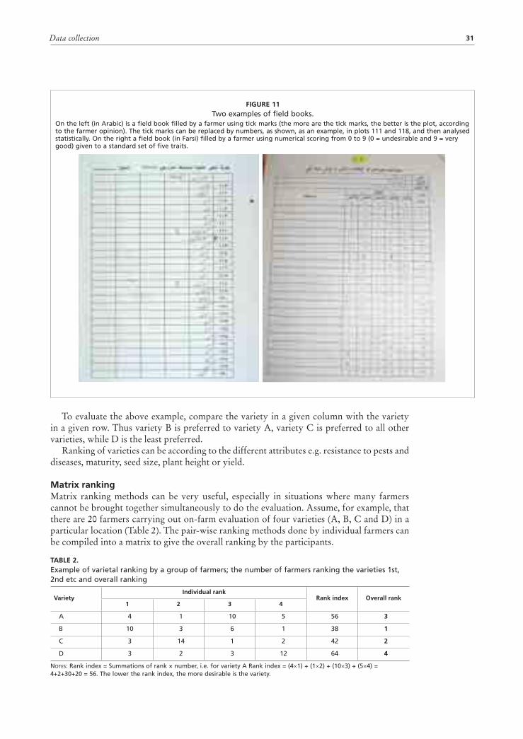
Data collection 31
To evaluate the above example, compare the variety in a given column with the variety in a given row. Thus variety B is preferred to variety A, variety C is preferred to all other varieties, while D is the least preferred.
Ranking of varieties can be according to the different attributes e.g. resistance to pests and diseases, maturity, seed size, plant height or yield.
Matrix rankingMatrix ranking methods can be very useful, especially in situations where many farmers cannot be brought together simultaneously to do the evaluation. Assume, for example, that there are 20 farmers carrying out on-farm evaluation of four varieties (A, B, C and D) in a particular location (Table 2). The pair-wise ranking methods done by individual farmers can be compiled into a matrix to give the overall ranking by the participants.
TABLE 2. Example of varietal ranking by a group of farmers; the number of farmers ranking the varieties 1st, 2nd etc and overall ranking
VarietyIndividual rank
Rank index Overall rank1 2 3 4
A 4 1 10 5 56 3
B 10 3 6 1 38 1
C 3 14 1 2 42 2
D 3 2 3 12 64 4
NOTES: Rank index = Summations of rank × number, i.e. for variety A Rank index = (4×1) + (1×2) + (10×3) + (5×4) = 4+2+30+20 = 56. The lower the rank index, the more desirable is the variety.
FIGURE 11Two examples of field books.
On the left (in Arabic) is a field book filled by a farmer using tick marks (the more are the tick marks, the better is the plot, according to the farmer opinion). The tick marks can be replaced by numbers, as shown, as an example, in plots 111 and 118, and then analysed statistically. On the right a field book (in Farsi) filled by a farmer using numerical scoring from 0 to 9 (0 = undesirable and 9 = very good) given to a standard set of five traits.


33
Experimental designs for PPB trials
Table 3 shows some experimental designs that can be used for the various stages of a participatory programme. The choice of the designs is dictated by (1) the amount of seed available in the various stages, (2) the average farm size in the target area, and (3) the need to find a compromise between offering to farmers as many choices as possible while keeping the total number of plots to a manageable size.
STAGE 1 TRIALSThe first stage of PPB is usually represented by trials composed of the same set of entries planted in as many locations as appropriate to represent the selection environment. In some cases, where there are strong differences in farmers’ preferences in different areas of the same country, it is advisable to prepare different trials with different types of germplasm. In both cases, the trials should have a different randomization in each location.
In Stage 1, when the total number of new entries tested vary (in our projects) between as few as 50 to as many as 160 at each location, a compromise must be sought between the plot size and the number of locations. This compromise is reached by sacrificing replications in favour of locations, as done in most CPB in the initial stages (Portmann and Ketata, 1997) in recognition that in this stage of the breeding programme ranking of genotypes is more important that predicting their yields (Kempton and Gleeson, 1997) and the G×E variance is larger than the experimental error variance; these trials can be grown using from one to four checks repeated a sufficient number of times to have at least 30 degrees of freedom for the estimate of the error variance. Examples are trials with 167 entries and 2 checks repeated 16 and 17 times, respectively, or trials with 165 entries and 3 checks repeated 11, 12 and 12 times respectively. In both cases the resulting 200 plots are arranged in a rectangular grid of rows and columns with the possible arrangements (4 rows × 50 columns, 8 rows and 25 columns, and 20 rows and 10 columns) shown in Figure 12. These different layouts may be suitable at different locations. The various arrangements allow a certain degree of flexibility in adapting the trial to various field shapes even though, unless there are severe restrictions, the 20 rows × 10 columns arrangement should be preferred. Figure 12 does not show the border plots, which should always surround the entire trial no matter what the layout is.
In this type of trial, the choice of the checks is important because they must represent a reference for the farmers during the selection process, they must provide an unbiased estimate of the experimental error and, in the long term, they can be used to estimate response to selection. Therefore, when they are chosen, one has to consider that changing them later
TABLE 3. Experimental designs in PPB trialsType and characteristics of trial Experimental design
Stage 1 (several entries, little seed available per entry)
Unreplicated with systematic checks or partially replicated (p –rep) in rows and columns or incomplete blocks in two replications in rows and columns
Stage 2 (fewer entries, more seed available per entry)
Incomplete blocks in two replications in rows and columns
Stage 3 (a few entries, much more seed available per entry)
Incomplete blocks in two replications in rows and columns
Stage 4 (2-4 entries, a large amount of seed available per entry)
RCBD with individual farms as replications

Plant breeding with farmers – a technical manual34
in the course of the programme implies a loss of information. Usually, farmers will insist that the local landrace(s) be included as check(s). Varieties that are candidates for release, if adopted by some farmers, can also be added.
The design shown in Figure 12 can be improved by replicating only part of the entries and not all as in a typical randomized complete block design (RCBD). For example, if in Stage 1 it is decided to test 160 entries, one can plant the 40 entries with more seed available twice (Figure 13). The entries that are replicated twice do not need to be the same in every village. Only we need to make sure that the resulting block design remains connected, which means that one can reach from one entry to another through blocks containing common entries with one or the other. These trials are partially replicated because only part of the entries or treatments is replicated or p-rep designs because they use replicated plots only for a portion p of the entries (Cullis, Smith and Coombes, 2006).
Ideally the replicated entries should be present in as many columns and rows as possible and will provide an estimate of the error variance. The improvement over the unreplicated design
FIGURE 12Three possible layouts of an unreplicated design with systematic checks and 200 plots.

Experimental designs for PPB trials 35
is associated with the fact that, first, in this case the error is estimated using a wider range of genotypes as compared with the few in the previous case, and, second, the error is estimated using breeding lines (which are the object of selection) rather than the checks that are not part of the selection process. One additional advantage of the partially replicated design is a more efficient use of the seed resources. In fact it is quite common in the first stages of a breeding programme to have different amount of seed for the different entries. Since the entry with the smallest amount of seed dictates the plot size and the number of locations, only part of the seed of all the other entries will be used and as consequence a large amount of seed is usually wasted. There could be cases where none of the layouts shown in Figures 12 and 13 fit the size of the farm where the trial should be planted. This is often the case of communities where each individual farmer has a very small farm. The danger in those conditions is to single out as participants those few farmers with enough land to host the trial. This is not necessarily bad if the farm size is the only difference between large and small farmers. However, usually large farmers are also using agronomic practices too expensive for small farmers or not suitable to small fields, and therefore the large farmers’ fields do not represent the majority of farmers in the community.
One possible solution is to layout the trial on an area that covers more than one farmer’s fields, an example of which is shown in Figure 14, where one of the 3 arrangements shown in Figure 12 or the trial shown in Figure 13 is planted on an area which embraces three different farmers’ fields.
If the solution shown in Figure 14 is not feasible because, for example, farmers’ fields are separated by physical obstacles such as trees or channels or walls, or are at different levels as
FIGURE 13 One of the two possible layouts of a partially replicated design: the plots with the replicated
entries are the red squares. The other two possible layouts are as shown in Figure 12.

Plant breeding with farmers – a technical manual36
in terrace-type agriculture, or have been planted with different crops the year before, then it is still possible to use a relatively large Stage 1 trial by using a replicated incomplete block design, an example of which is shown in Figure 15.
Incomplete block designs have the objective of controlling the plot-to-plot variation and ideally they should allow the comparisons for all pairs of genotypes (Mead, 1997); this is rarely achievable with a large number of genotypes but only few replications. Resolvable designs are designs in complete replicated blocks, with each replicate split into small incomplete blocks. Lattice designs are a special type of resolvable incomplete blocks where the number of genotypes g is the square of an integer and the block size is √g. The introduction of alpha-designs (Patterson and Williams, 1976) removed the restrictions in term of number of genotypes. The advantage of an incomplete block design is that each incomplete block (a sequence of 20 plots in the example shown in Figure 15) is an independent unit and therefore can be allocated to a different field from each of the other incomplete blocks within the same environment. The number of incomplete blocks that can be planted on each farm depends only on the farm size, and therefore there can be fields with anywhere from 1 to 5 incomplete blocks based on the field trials I have dealt with. It is also possible that one full replication is planted by a large farmer and the 10 incomplete blocks of the other replication with 10 different farmers. The disadvantages of this layout are two-fold: first, the restriction that the total number of entries (g) is a multiple of the block size (k) so that g = sk where s = number of incomplete block per replication, in which case the design is easier; however, there are certain numbers of entries for which g ≠ sk where the design is not easily available; and, second, the loss of the row and column design which, as we will see later, is needed for a spatial analysis.
One additional possibility to cope with small farms is to subdivide the trial into a number of trials of a size corresponding to available farm sizes. By making sure that all these smaller
FIGURE 14The example of a large 1st stage PPB trial too large to be hosted by an individual farmer, but that can
be planted on a homogeneous piece of land spreading across different farmers’ fields
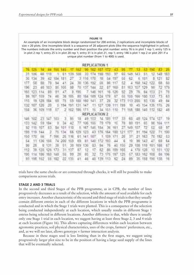
Experimental designs for PPB trials 37
trials have the same checks or are connected through checks, it will still be possible to make comparisons across trials.
STAGE 2 AND 3 TRIALSIn the second and third Stages of the PPB programme, as in CPB, the number of lines progressively decreases as a result of the selection, while the amount of seed available for each entry increases. Another characteristic of the second and third stage of trials is that they usually contain different entries in each of the different locations in which the PPB programme is conducted and in which the Stage 1 trials were planted. This is a consequence of the selection being conducted independently at each location, which usually results in different Stage 1 entries being selected in different locations. Another difference is that, while there is usually only one Stage 1 trial in each location, we suggest having at least three Stage 2, 3 and 4 trials at each location (Figure 16). This allows capturing differences within each location between agronomic practices, soil physical characteristics, uses of the crops, farmers’ preferences, etc., and, as we will see later, allows genotype × farmer interaction analysis.
Because in these stages seed is less limiting than in the first stages, we suggest using progressively larger plot size to be in the position of having a large seed supply of the lines that will be eventually selected.
FIGURE 15An example of an incomplete block design randomized for 200 entries, 2 replications and incomplete blocks of
size = 20 plots. One incomplete block is a sequence of 20 adjacent plots (like the sequence highlighted in yellow). The numbers indicate the entry number and their position the plot number: entry 76 is in plot 1 rep 1; entry 125 is
in plot 2 rep 1; entry 25 is in plot 20 rep 1; entry 31 is in plot 21, rep 1; entry 146 is plot 1 rep 2 or plot 201 if a unique plot number (from 1 to 400) is used.
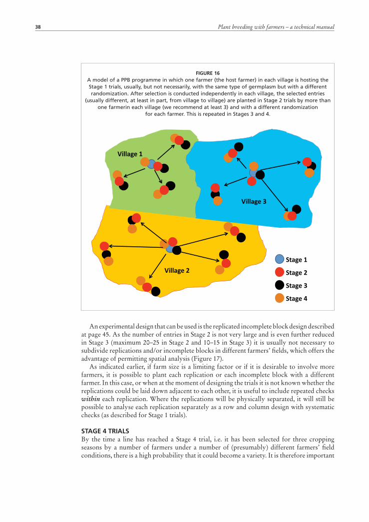
Plant breeding with farmers – a technical manual38
An experimental design that can be used is the replicated incomplete block design described at page 45. As the number of entries in Stage 2 is not very large and is even further reduced in Stage 3 (maximum 20–25 in Stage 2 and 10–15 in Stage 3) it is usually not necessary to subdivide replications and/or incomplete blocks in different farmers’ fields, which offers the advantage of permitting spatial analysis (Figure 17).
As indicated earlier, if farm size is a limiting factor or if it is desirable to involve more farmers, it is possible to plant each replication or each incomplete block with a different farmer. In this case, or when at the moment of designing the trials it is not known whether the replications could be laid down adjacent to each other, it is useful to include repeated checks within each replication. Where the replications will be physically separated, it will still be possible to analyse each replication separately as a row and column design with systematic checks (as described for Stage 1 trials).
STAGE 4 TRIALSBy the time a line has reached a Stage 4 trial, i.e. it has been selected for three cropping seasons by a number of farmers under a number of (presumably) different farmers’ field conditions, there is a high probability that it could become a variety. It is therefore important
FIGURE 16A model of a PPB programme in which one farmer (the host farmer) in each village is hosting the Stage 1 trials, usually, but not necessarily, with the same type of germplasm but with a different randomization. After selection is conducted independently in each village, the selected entries
(usually different, at least in part, from village to village) are planted in Stage 2 trials by more than one farmerin each village (we recommend at least 3) and with a different randomization
for each farmer. This is repeated in Stages 3 and 4.

Experimental designs for PPB trials 39
to organize and implement an aggressive seed multiplication programme for those lines that have been progressively selected in each of the previous stages.
If the PPB programme develops as collaboration between a research institution and the farmers, the seed multiplication can easily be done under the optimum management conditions of the research station. As the programme proceeds, the seed of the lines which are not selected can be used for the in-kind compensation, while the seed of the lines that are selected is used to grow progressively larger plots or to grow Stage 2, 3 and 4 trials at more locations and with more farmers.
If the research station facilities are not available to the PPB programme, the responsibility for seed production can be taken up by one of the willing or progressive farmers. In situations where few farmers own relatively large farms while most farmers own small farms, the former can take the responsibility for seed production on behalf of the entire community as long as issues of access and benefit sharing are discussed and clarified beforehand.
Assuming that a relatively large amount of seed is available for the lines selected from Stage 3 and to be planted in Stage 4 (25–50 kg in the case of cereal crops), the design that is suggested is the RCBD, in which each farmer plants only one replication (Figure 18) and with the largest possible plot size that the amount of seed available allows. In this way, Stage 4 will provide one more set of data to be used to decide which line(s) deserve(s) to become a variety, and at the same time will produce a sufficient amount of seed for a wider distribution of the variety. The layout shown in Figure 18 can be easily used in PVS trials.
FIGURE 17An example of a Stage 2 (or Stage 3) replicated (2 replications) trial with 10 entries arranged in
incomplete blocks (block size = 5, each block is represented by a different colour) with two layouts: 2 rows (each row = 1 replication) and 10 columns (A); and 4 rows (2 rows = 1 replication)
and 5 columns (B). The numbers indicate the plot sequence.
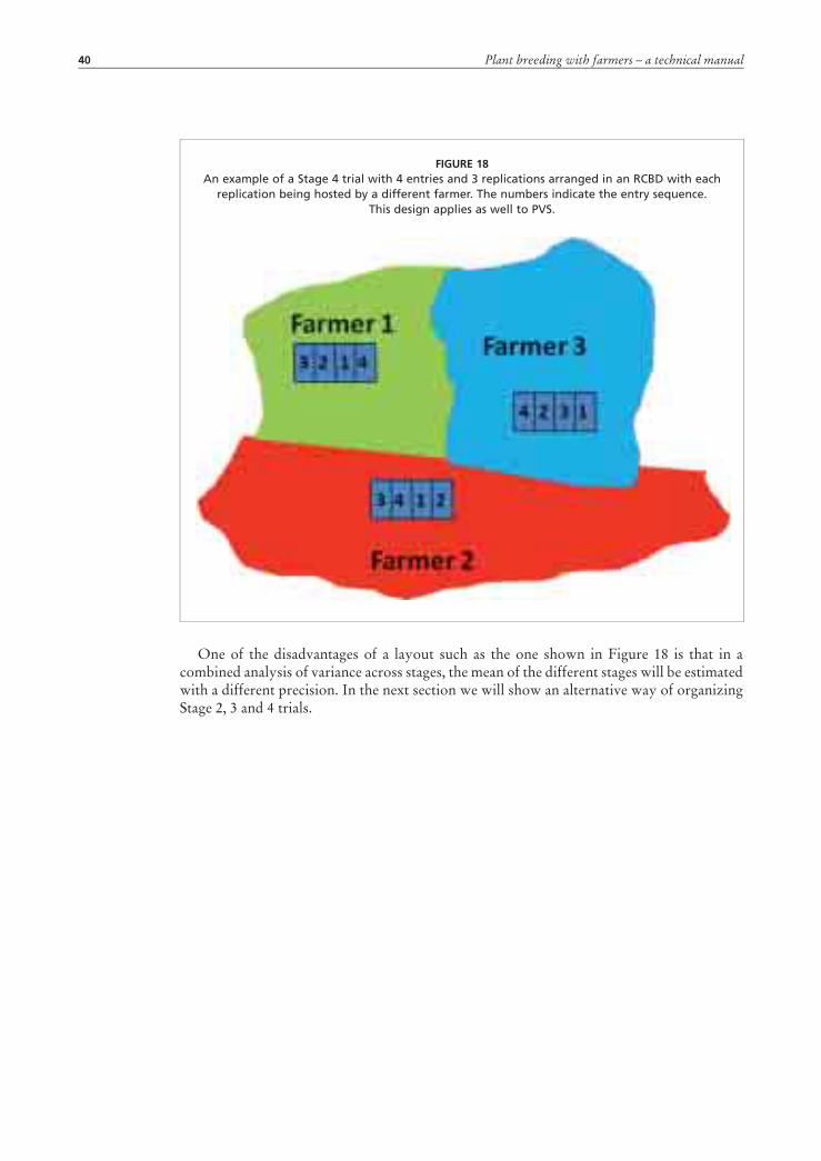
Plant breeding with farmers – a technical manual40
One of the disadvantages of a layout such as the one shown in Figure 18 is that in a combined analysis of variance across stages, the mean of the different stages will be estimated with a different precision. In the next section we will show an alternative way of organizing Stage 2, 3 and 4 trials.
FIGURE 18An example of a Stage 4 trial with 4 entries and 3 replications arranged in an RCBD with each
replication being hosted by a different farmer. The numbers indicate the entry sequence. This design applies as well to PVS.
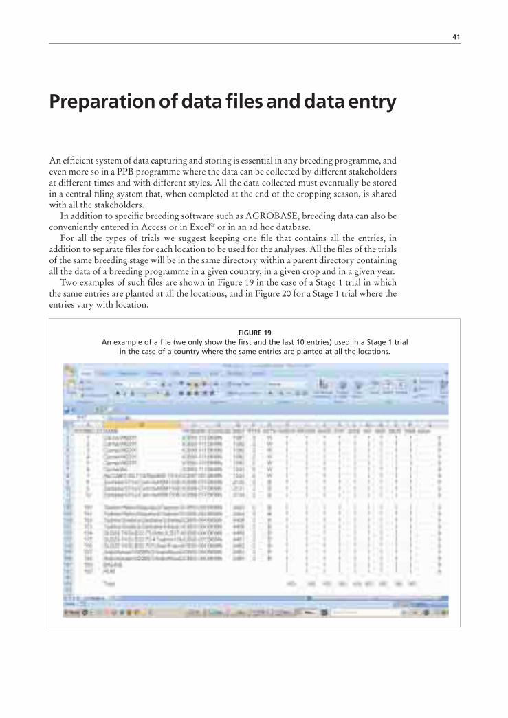
41
Preparation of data files and data entry
An efficient system of data capturing and storing is essential in any breeding programme, and even more so in a PPB programme where the data can be collected by different stakeholders at different times and with different styles. All the data collected must eventually be stored in a central filing system that, when completed at the end of the cropping season, is shared with all the stakeholders.
In addition to specific breeding software such as AGROBASE, breeding data can also be conveniently entered in Access or in Excel® or in an ad hoc database.
For all the types of trials we suggest keeping one file that contains all the entries, in addition to separate files for each location to be used for the analyses. All the files of the trials of the same breeding stage will be in the same directory within a parent directory containing all the data of a breeding programme in a given country, in a given crop and in a given year.
Two examples of such files are shown in Figure 19 in the case of a Stage 1 trial in which the same entries are planted at all the locations, and in Figure 20 for a Stage 1 trial where the entries vary with location.
FIGURE 19An example of a file (we only show the first and the last 10 entries) used in a Stage 1 trial
in the case of a country where the same entries are planted at all the locations.

Plant breeding with farmers – a technical manual42
The files we use have a standard structure: • a unique genotype identification number (column A) – we suggest using the number
used in the seed multiplication plots on-station or on-farm, for reasons that will be clearer later;
• entry name (column B);• pedigree (column C); and • source and source number (the number of these last two columns depends on the
number of years the material has been on station before being used in the Stage 1 trials). The data collected on station (for example on disease and insect resistance) can also be
part of the file. In crops such as barley, where row type (RT: 2-row and 6-row coded as 2 and 6) and seed colour (SC: black and white coded as B and W) may considerably affect farmers’ preferences, this information is also noted in the file. The right-hand side of the file contains the information about the villages (in this case 9) in which the various entries are planted. The names of the villages are abbreviated to 2–3 digits with the addition of 09 as the indication of the year of the experiment (2009). In the case of Figure 19 all the entries are planted in each of the 9 villages, while in the case of Figure 20, although 160 entries are planted in each of the 7 villages (see totals on the bottom of columns CF to CL), the actual entries planted in each village differ as shown by the marginal totals in column CM. As a consequence the total
FIGURE 20An example of a file (we only show some of the entries) used in a Stage 1 trial in the case of a country where different entries are planted in different locations. The total number of entries is 311. The entries from 312 to
325 are checks (not necessarily the same in each village).

Preparation of data files and data entry 43
number of new entries tested in any given year can be fairly high (311 excluding the checks (numbers 312 to 325) in the case of the 2009 trials in Syria – see Figure 20).
The presence or absence of a given entry in the column corresponding to a given location is indicated by 1 or 0, respectively. Therefore, the list of entries planted, for example, in location AZ09 is simply obtained by sorting the file by column CF in descending order and by column A in ascending order and this is in fact the first step in the preparation of the data files. This will result in 9 files in the case of the Stage 1 trial shown in Figure 19 and in 7 files in case of the Stage 1 trial shown in Figure 20. It is obvious that in a case like the one in Figure 19 the entry number of a given genotype in each of the 9 locations will be the same as the unique identification number (FIT09INCJO), shown in column A. However, in a case like the one in Figure 20 this will not be true and the same entry number in two different locations may actually refer to different genotypes, which can then only be identified by using the unique identification number (FIT09IN) in column A.
Files such as those shown in Figure 19 and 20 are also very useful for the preparation of the seed for planting, particularly when different seed rates are used in the same village. To do this it is sufficient to add a number of columns equal to the number of locations with the amount of seed needed for each entry in each village in place of the 1’s. The marginal totals of these columns will be the amount of seed needed for that entry in all the trials. After adding the amount of seed needed for the seed multiplication plots we will have the total amount of seed needed for each entry.
Once the individual file for each individual location is ready, the next step is to randomize the entries in each location.
RANDOMIZATIONRandomization allows the unbiased assignment of treatments to experimental units (in this case of entries to the plots) and is a prerequisite for obtaining a valid estimate of the experimental error. One of the most common mistakes, besides replications, in the layout of breeding trials is to avoid the randomization in the first replication so that the plot order corresponds to the entry order, which is statistically incorrect. Another common mistake in Multi Environment (years and locations) Trials (MET) is to use the same randomization in all the locations within the same year.
AlphanalRandomization can be done with various programs or manually. A free and friendly MS-DOS software is ALPHANAL produced by the Scottish Agricultural Statistics Service. Although designed for alpha-designs (incomplete block designs) it can be conveniently used also for the randomization of unreplicated trials. After opening the directory “ALPHANAL” identify the two commands, ALPHAGEN.EXE and ALPHANAL.EXE, for the generation of randomizations plans and for data analysis, respectively. The limits of ALPHAGEN are 500 entries and 20 plots per incomplete block, which represents an advantage over the corresponding command in GenStat which allows a maximum of 100 entries. Figure 20 shows the main steps in using the program in the case of a trial with 160 entries in 200 plots.
To use ALPHAGEN for the randomization of unreplicated trials with systematic checks (known also as augmented designs) or for partially replicated trials, we consider each location as a replication, and the total number of plots as the number of treatments (= entries). In deciding the number of plots per incomplete block one should have already in mind the layout of the trial. In the case of 50 columns and 4 rows, arrangements can be either 5 or 10 incomplete blocks, because 50 cannot be divided by 20 and 25 is above the limits of the programme.
Once the parameters of the trials are fixed, the programme uses an iterative process to find the most efficient design (continue to answer “yes” to the question “Do you want to search

Plant breeding with farmers – a technical manual44
for a better design?” until the message “There are no more efficient designs of this size” is displayed) and produces a randomization plan which can be stored with a given name. Note that the efficiency of incomplete block design is a function of the number of comparisons between genotypes within the same incomplete block and will always be less than 1 because there will always be a number of comparisons between genotypes that are in different blocks.
In the case of replicated trials, as in Stage 2, 3 and 4 and regardless of whether the trials are a physical unit as in Figure 17, or planted by different farmers as incomplete blocks or complete replications (Figure 18), the randomization follows the same process as shown in Figure 21, with minor differences as shown in Figure 22.
Assuming a Stage 3 trial with 12 entries to be grown with 2 replications and 3 farmers, we will need to enter 6 as number of replications (= number of farmers × number of replications in each farmers’ field) (Figure 22). The full randomization plan with block size = 4 is shown in Figure 23. The number of incomplete blocks in this case could have been either 2, 3 4 or 6. Small incomplete blocks are usually associated with a greater precision but with a lower efficiency as the number of comparisons between entries in different incomplete blocks increases. One has also to consider possible restrictions imposed by field shape because it is not possible to break the physical unity of an incomplete block.
The major problem with conducting the randomization with ALPHAGEN is importing the text file into Excel® (see pages 47–53).
FIGURE 21Main steps in the randomization of an unreplicated Stage 1 PPB trial with 160 entries and
200 plots using the command ALPHAGEN in ALPHANAL.

Preparation of data files and data entry 45
DIGGerDiGGer is a program that finds efficient designs for non-factorial experiments with experimental units that can be specified as a rectangular array and under specified correlation structures (Coombes, 2006; Cullis, Smith and Coombes, 2006). DiGGer can find optimal or near-optimal incomplete block designs, row-column designs and spatial designs. The program, together with manuals and examples, can be freely downloaded from http://www.austatgen.org/files/software/downloads/
DiGGer was developed for cereal variety trials with plots in rectangular arrays, but can be used for any design that can be described in row and column layouts. Designs may have treatments with unequal replication and may have missing plots. Designs may be optimized for comparisons between groups of treatments.
DiGGer is available as a standalone executable and as an R package. The standalone version runs from an input file or interactively in a command window. The
FIGURE 22Main steps in the randomization of a replicated Stage 2, 3 or 4 trial with 2 replications, 12 entries and incomplete
blocks of size 4, using the command ALPHAGEN in ALPHANAL. The trial is grown by 3 farmers.
FIGURE 23Randomization of a Stage 3 trial using an incomplete
block design with 12 entries, 2 replications, incomplete blocks of size 4 planted by 3 farmers
in the same village.
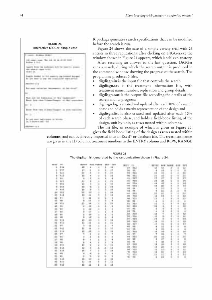
Plant breeding with farmers – a technical manual46
R package generates search specifications that can be modified before the search is run.
Figure 24 shows the case of a simple variety trial with 24 entries in three replications: after clicking on DIGGer.exe the window shown in Figure 24 appears, which is self-explanatory.
After receiving an answer to the last question, DiGGer runs a search, during which the search output is produced in the command window showing the progress of the search. The programme produces 5 files:• digdisgn.in is the input file that controls the search;• digdisgn.trt is the treatment information file, with
treatment name, number, replication and group details;• digdisgn.out is the output file recording the details of the
search and its progress;• digdisgn.log is created and updated after each 10% of a search
phase and holds a matrix representation of the design and • digdisgn.list is also created and updated after each 10%
of each search phase, and holds a field-book listing of the design, unit by unit, as rows nested within columns.
The .lst file, an example of which is given in Figure 25, gives the field-book listing of the design as rows nested within
columns, and can be directly imported into an Excel® or database file. The treatment names are given in the ID column, treatment numbers in the ENTRY column and ROW, RANGE
FIGURE 24 Interactive DiGGer: simple case
FIGURE 25The digdisgn.lst generated by the randomization shown in Figure 24.
Preparation of data files and data entry 47
(column) and REP (replicate) details. The TRT column holds design numbers used by DiGGer and these are the numbers that appear in the .log file.
The software can handle a maximum of 1500 experimental units (treatment × replications). In the case of partially replicated designs the PRDiGGer function uses blocking
specifications to even out the placement of unreplicated treatments and control treatments throughout a design. The function is aimed at designs with some unreplicated treatments. The function requires the minimum input of treatment information (typically a .csv file) with “Name”, “Entry No.”, “No.Reps”, “Group”, the dimensions of the design and the blocking sequences, and produces a colour-coded plot of the design and a .csv file with the field-book listing of the design.
At the time of writing this manual, the PRDiGGer function has not been yet included in the DiGGer package and for its use we suggest contacting Neil Coombes ([email protected]).
LUMPING TOGETHER TRIALS OF DIFFERENT STAGESOne way of increasing the precision of the field trials is to combine a number of different stages into a single trial. For example, in the model of PPB we just described, we could have one trial including all the entries tested in the 1st, 2nd, 3rd and 4th Stages using the same plot size of Stage 1 or, probably more realistically, two trials, one corresponding to Stage 1 as described earlier, and one including all the entries tested in the 2nd, 3rd and 4th Stages using a common plot size. Obvious advantages of lumping together different trials are, first, the assessment of all the entries in the same environment, and, second, saving on land, or alternatively increasing the number of test entries with a relative reduction in the number of checks..
Figure 26 shows a real case as an example: there are three trials (Stage 2 with 15 entries and 5 checks; Stage 3 with 6 entries and 4 checks; and Stage 4 with 3 entries and four checks = a total of 37 entries) grown side by side in the same farmer’s field.
In the upper part of Figure 26, the three trials have been randomized independently with ALPHAGEN, and each square shows the entry number with those of the checks in colour. It will be noticed that most checks are common to all the trials; when the randomization was done with DIGGer, again independently in each trial, the spatial distribution of the checks slightly improved (in the randomization with ALPHAGEN there is a gap of 6 columns with no checks while with the DIGGER the largest interval with no checks is three columns. In both cases, the design will not be able to cope with, for example, a fertility gradient increasing linearly from Stage 2 to Stage 4 or vice versa, which will cause a bias in comparing entries from different trials when the analysis is conducted on each trial separately.
When the entries of the three trials are combined together (but without losing their identity, as shown in column B of Figure 27), the first effect is a reduction in the total number of entries due to a reduction in the number of duplicated checks across stages. This implies a reduction in the area needed for the trials but also, more importantly, the Best Linear Unbiased Predictors (BLUPs) of the entries performance or effects are estimated regardless of the stage to which they belong. The new combined trial can now be randomized either with ALPHAGEN or DIGGER, and the result is shown in Figure 28. Also in this case it is evident that a more uniform spreading of the checks across the trial is obtained with DIGGer compared with ALPHAGEN.
The only drawback of lumping together the entries of different trials is that the breeder loses the visual comparison of the entries belonging to the different stages of the breeding programme.
After the analysis, described under “Data Analysis” (page 57) the entries can be again separated according to the stage to which they belong.

Plant breeding with farmers – a technical manual48
FIG
UR
E 26
An
exa
mp
le o
f St
age
2, S
tag
e 3
and
Sta
ge
4 tr
ials
gro
wn
sep
arat
ely
wit
h e
ntr
ies
ran
do
miz
ed
wit
h A
LPH
AG
EN (
up
per
par
t) a
nd
DIG
GER
(lo
wer
par
t)
ind
epen
den
tly
in e
ach
tri
al. T
he
nu
mb
ers
in t
he
squ
ares
are
th
e en
try
nu
mb
ers,
wit
h t
he
chec
ks s
ho
wn
wit
h c
olo
urs
(sa
me
colo
ur
for
the
sam
e ch
eck)
. Th
e th
ree
tria
ls a
re g
row
n s
ide
by
sid
e in
th
e sa
me
farm
er’s
fie
ld.

Preparation of data files and data entry 49
PREPARATION OF A FILE FOR DATA RECORDINGUnreplicated or partially replicated trialsThe randomization plan, like the one shown in Figure 15, can be opened with Word and imported into the Excel® file keeping in mind that each replication corresponds to a different location and that the numbers that appear in the randomization files are entry numbers and the position is the plot number. So entry 76 is in plot 1, entry 25 is in plot 20, entry 31 in plot 21 and so on . Therefore, still using the example with 160 entries and 200 plots, one should proceed as follows:1. Open the file corresponding to a given location. This file should have already a sheet
called ‘entries’ (Figure 29).2. Insert a new sheet, which we usually name “fldbook” (an abbreviation for ‘field book’)
– this will eventually be the sheet for data entry.3. Enter a column with the header “plot” and fill it with numbers from 1 to 200.
FIGURE 27 The entries in Stage 2, Stage 3 and Stage 4 combined in a common file with the same checks used in the separate
trials. The entries have been renumbered. It will be noticed that the total number of entries has gone down from 37 to 30 entries.

Plant breeding with farmers – a technical manual50
4. Import one of the randomization files and with “paste special and transpose” create a column with entry numbers (header = entry) close to the column with plot numbers. During this operation one should always remember that the plot numbers always start from the left of the randomization plan. In other words, each row in the randomization plan becomes a column under the previous one under the header entry. These steps can be conveniently and rapidly performed using a macro in Excel®.
5. Sort the file by ascending order for the column “entry”. Since we actually have only 160 entries and not 200, we will need to modify this column. The modification depends on whether the trial uses systematic checks or is partially replicated, so for5A. systematic checks, let us suppose that we are using two systematic checks, which
are entry 159 and entry 160, as in the example shown in Figure 19. In this case we will replace, in the column entry, all the entry numbers from 159 to 179 with 159, and the corresponding plots will receive the entry BALADI (the local check). Similarly, we will replace the entry numbers from 180 to 200 with 160, and the corresponding plots will receive the entry RUM (the improved check); while for
FIGURE 28The Stage 2, Stage 3 and Stage 4 combined in a common trial randomized with ALPHANAL (above) and
DIGGER (below).

Preparation of data files and data entry 51
5B. partially replicated design the entry numbers from 161 to 200 are replaced by the entry numbers of those 40 entries (with entry number < or = 160) for which there is enough seed to plant two plots.
6. Once step 5 is completed and regardless whether we used option 5A or 5B above, we copy the relevant columns from the sheet “entry” into the sheet “fldbook”, making sure that the names match the entry numbers. For the reasons explained earlier, it is very important to also copy the column with the unique identification number. All these columns should be pasted at the right side of the column “entry”.
7. Sort the file by ascending order for the column “plot”.8. Insert three new columns. The first named “trial”, with a unique numerical value indicating
the village, to be inserted at the left of the column “plot”; and two named “row” and “column” to be inserted between the columns “plot” and “entry”.
9. Fill “row” and “column” according to the layout chosen among those shown in Figures 12 and 13.
10. Repeat steps 1 to 9 for every location.
FIGURE 29An example of a fieldbook sheet in a data file of a Stage 1 trial with 160 entries and 200
plots in 4 rows and 60 columns. Only the first and the last 11 rows are shown.
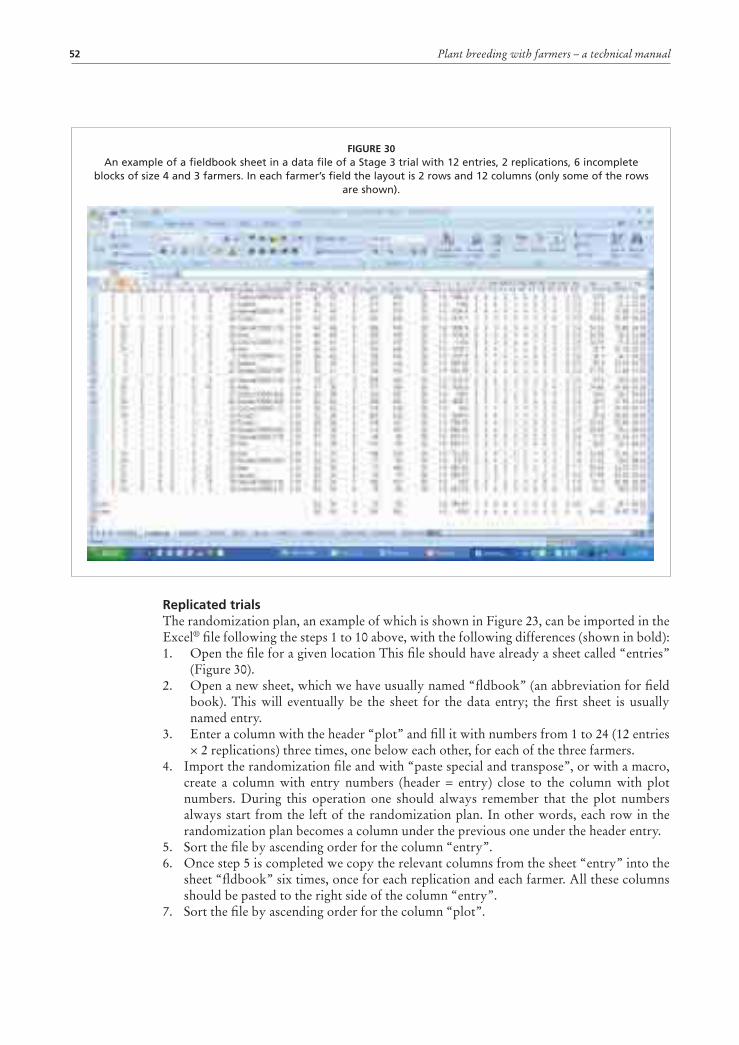
Plant breeding with farmers – a technical manual52
FIGURE 30An example of a fieldbook sheet in a data file of a Stage 3 trial with 12 entries, 2 replications, 6 incomplete
blocks of size 4 and 3 farmers. In each farmer’s field the layout is 2 rows and 12 columns (only some of the rows are shown).
Replicated trialsThe randomization plan, an example of which is shown in Figure 23, can be imported in the Excel® file following the steps 1 to 10 above, with the following differences (shown in bold):1. Open the file for a given location This file should have already a sheet called “entries”
(Figure 30).2. Open a new sheet, which we have usually named “fldbook” (an abbreviation for field
book). This will eventually be the sheet for the data entry; the first sheet is usually named entry.
3. Enter a column with the header “plot” and fill it with numbers from 1 to 24 (12 entries × 2 replications) three times, one below each other, for each of the three farmers.
4. Import the randomization file and with “paste special and transpose”, or with a macro, create a column with entry numbers (header = entry) close to the column with plot numbers. During this operation one should always remember that the plot numbers always start from the left of the randomization plan. In other words, each row in the randomization plan becomes a column under the previous one under the header entry.
5. Sort the file by ascending order for the column “entry”.6. Once step 5 is completed we copy the relevant columns from the sheet “entry” into the
sheet “fldbook” six times, once for each replication and each farmer. All these columns should be pasted to the right side of the column “entry”.
7. Sort the file by ascending order for the column “plot”.

Preparation of data files and data entry 53
As we have seen earlier, steps 1–7 are not necessary if the randomization is done with DIGGER or GenStat.
The next steps will depend on whether the trial is a physical unit or not. If the trial is a physical unit, then the steps to follow are (Figure 30):8. Insert five new columns. The first named “farmer”, with a numerical value indicating the
farmer (in our example, 1 for rows 2 to 25 [row 1 is the header], 2 for rows 26 to 49 and 3 for rows 50 to 73) to be inserted at the left of the column “plot”, and four columns named “block”, “sblock”, “row” and “column” to be inserted between “plot” and “entry”. The column “block” has to be filled with the code for replication (in our example it will be 1 for rows 2 to 13; 26 to 37; and 50 to 61; with 2 for rows 14 to 25; 38 to 49; and 62 to 73) and the column “sblock” has to be filled with the code for the incomplete blocks (in our example the values are from 1 to 6 for each farmer).
9. Fill “row” and “column” according to the layout, as indicated in Figure 17.If the trial is not a physical unit (Figure 18) then the steps to follow are:
8. Insert three new columns: The first named “trial”, with the numerical code for the village; the second named “farmer”, with a numerical value indicating the farmer (in our example this will be 1 for rows 2 to 25 [row 1 is the header]; 2 for rows 26 to 49; and 3 for rows 50 to 73) to be inserted to the left of the column “plot”, and the third column, named “block”, to be filled with the code for replication (in our example it will be 1 for rows 2 to 13; 26 to 37; and 50 to 61; with 2 for rows 14 to 25; 38 to 49; and 62 to 73).
As we will see later the column “plots” is not required for the analysis but it is useful to keep it in the “fldbook” to facilitate data collection.
The preparation of the file, in this case a text file, is much simpler if the data is analysed with ALPHANAL, and this will be illustrated in the section on data analysis.
DATA ENTRYThe sheet "fldbook" prepared according to the steps listed above can be printed for manual data recording in the field or in the lab, or can be saved in a palmtop for electronic recording of the data.
In the first case, the data have to be entered manually in the sheet “fldbook”, while in the second they will be transferred by connecting the palmtop to the desktop or the laptop. In either case it is strongly recommended that the data be entered or transferred IMMEDIATELY AFTER BEING COLLECTED FROM THE FIELD. Once entered in the computer, it is suggested to calculate minimum and maximum or to rank them, to verify that there are no obvious mistakes. Even better is to analyse them, because this can easily reveal mistakes either in recording the data from the field or in entering them manually. A mistake discovered when the crop is still in the field can be easily fixed by going back to the field and by measuring again the plot(s) with value(s) which look suspicious or which are obviously wrong.
In the “fldbook” sheet it is important to use the same abbreviations and units as in the sheet “traits” (Figure 10). Additional information, such as missing plots, plot damage (by farm animals, ants, etc.), can be entered in a special column “notes”. In the case of the yield data, it is recommended to enter a column with the plot size and one with the area harvested, regardless whether the two differ or not . The principle in organizing this important sheet in the file is that it should be as transparent as possible to those who are not familiar with the trial.
Examples of the “fldbook” sheet in a data file of an unreplicated trial (Stage 1) and of a replicated trial (Stage 3) are given in Figures 29 and 30, respectively.
A number of features shown in the two Figures are worth mentioning. Firstly, it will be noticed that the entry number (column G in Figure 29 and column I in Figure 30) does not

Plant breeding with farmers – a technical manual54
necessarily correspond to the unique identification number of the genotype (column H in Figure 29 and J in Figure 30) for the reasons mentioned before. Secondly, as one of characters which are important to farmers in the case of barley (and presumably also of other cereals) is spike length, we take two measures of plant height, one from ground level to the bottom of the spike (PlHt_B_cm), and one from ground level to top of the spike excluding the awns (PlHt_T_cm); spike length (SL_cm) is then derived with a formula (column P - column O). This method does not have any advantage in case of manual note taking. However, in the case of electronic capturing of the data, the spike length is automatically calculated plot by plot as the other two measures are recorded, as an additional way to check the data. Thirdly, grain yield is recorded on one sample of 1.6 m2 as g/plot in the Stage 1 trial (column R in Figure 29) and on two samples (because of larger plots) of 1.6 m2 in the Stage 3 trial (columns T and U in Figure 30). Grain yield in kg/ha (columns U in Figure 29 and X in Figure 30) is obtained by dividing column R by plot size (column S) and multiplying by 10 in Stage 1 trials and by dividing the mean of the two samples by the plot size and multiplying by 10 in Stage 3 trials.
Columns V to AE (Figure 29) and Y to AH (Figure 30) contain the scores (from 0 = bad, to 4 = very good) given by individual farmers (in this case 10, but the number is obviously variable from village to village), and their average (FS) is in columns AF and AI, respectively. Eventually 1000-kernel weight in grams (TKW) is in column AG in Figure 29 while, since we have two samples for grain yield in the Stage 3 trial (Figure 30), 1000 kernel weight is measured independently in the two samples (columns AJ and AK) and their mean is in column AL.
FIGURE 31An example of a “fldbook” sheet in a data file of a Stage 4 trial with 9 entries and 2 replications
with one replication planted with one farmer and the second with another farmer.

Preparation of data files and data entry 55
In rows 204 and 205 of Figure 29 and in rows 78 and 79 of Figure 30 are the minimum and maximum for the values in each of the relevant columns. As mentioned earlier this is a powerful and easy way to detect a number of mistakes.
An example of the “fldbook” sheet in a data file of a Stage 4 trial with replications planted with different farmers is shown in Figure 31. The structure of the file is considerably simpler than those considered so far. The sheet “fldbook” has one column with the code for the village , one for the plot number, one for the entry number, one for the unique identification number (= plot number in the seed increase), and one for the farmer (which in this case is equivalent to the replication code).
These columns will be followed by those with the data, which are similar to those discussed earlier (see Figure 23 and 24) with the difference that, because now the plots are much larger, grain yield and 1000 kernel weight are measured on three samples each (columns N, O and P for grain yield in g/plot and columns AE, AF and AG for 1000-kernel weight in g).
The “fldbook” sheet shown in Figure 31 may also be used in Stage 2 and 3 trials when it is not possible to keep the trial as a physical unit.
Before leaving this topic, it worth mentioning that is very useful (for reasons that will be clear in the section on data analysis) to:
• Use the shortest, but still meaningful, possible abbreviation as a header for each variable.
• Always use the same abbreviation for the same variable.• Always use the same sequence of variables. The actual sequence is important for plot,
row, column and entry but not for the variables. However, once a given sequence for the variables is decided, always using the same sequence saves a lot of work during the subsequent data management analysis and data reporting.
The operations described above apply with only minor differences for a range of statistical analysis using a set of modules running in GenStat and available on request from the author.
DATA STORAGESafe data storage is a major issue in plant breeding programmes. Examples of strategies that can be used to reduce to a minimum the risk of data loss are frequent backups, storage of data in external disk drives, and storage of data in at least one computer never connected with networks or the Internet to reduce the probability of introducing viruses.

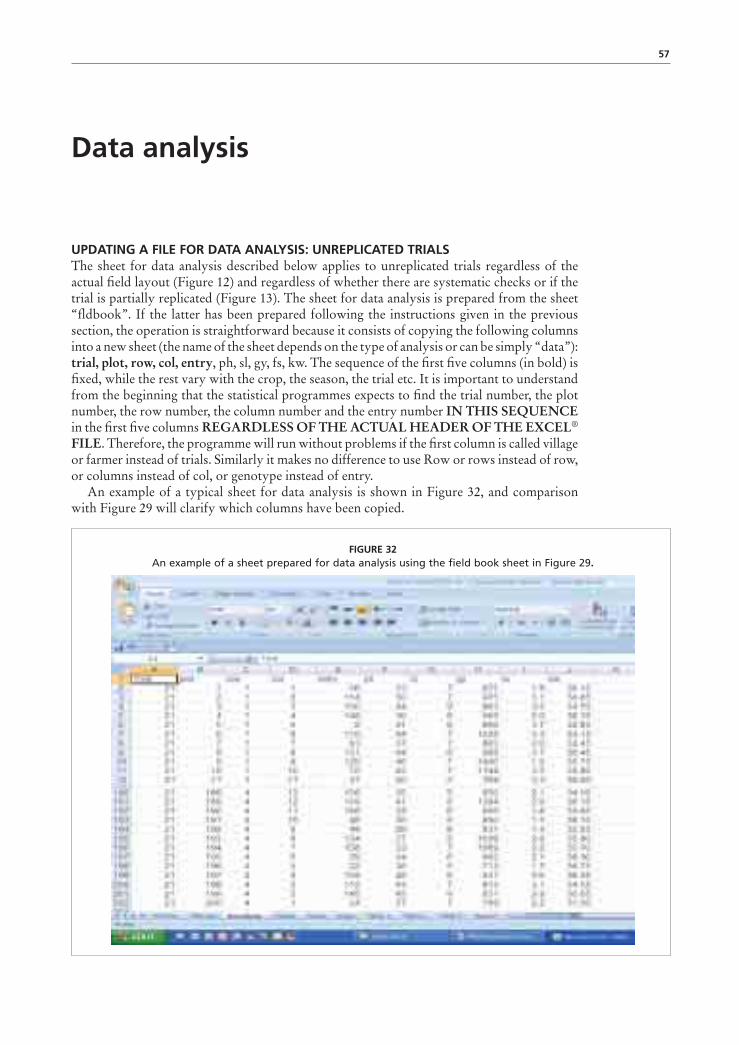
57
Data analysis
UPDATING A FILE FOR DATA ANALYSIS: UNREPLICATED TRIALSThe sheet for data analysis described below applies to unreplicated trials regardless of the actual field layout (Figure 12) and regardless of whether there are systematic checks or if the trial is partially replicated (Figure 13). The sheet for data analysis is prepared from the sheet “fldbook”. If the latter has been prepared following the instructions given in the previous section, the operation is straightforward because it consists of copying the following columns into a new sheet (the name of the sheet depends on the type of analysis or can be simply “data”): trial, plot, row, col, entry, ph, sl, gy, fs, kw. The sequence of the first five columns (in bold) is fixed, while the rest vary with the crop, the season, the trial etc. It is important to understand from the beginning that the statistical programmes expects to find the trial number, the plot number, the row number, the column number and the entry number IN THIS SEQUENCE in the first five columns REGARDLESS OF THE ACTUAL HEADER OF THE EXCEL® FILE. Therefore, the programme will run without problems if the first column is called village or farmer instead of trials. Similarly it makes no difference to use Row or rows instead of row, or columns instead of col, or genotype instead of entry.
An example of a typical sheet for data analysis is shown in Figure 32, and comparison with Figure 29 will clarify which columns have been copied.
FIGURE 32An example of a sheet prepared for data analysis using the field book sheet in Figure 29.
Plant breeding with farmers – a technical manual58
SPATIAL ANALYSIS OF AN UNREPLICATED TRIALOnce the data are prepared as shown in Figure 32, it is possible to proceed to the analysis following the steps below:
1. Open the directory “id_2002006 SPUR Spatial Analysis of Unreplicated Trials”. To fully understand the theory behind this section please consult Singh et al. (2003);
2. Open the file “DataSPUR.txt”. The first part of the file is simply a set of instructions, most of which have been given above. The new instructions are those listed as inputs, meaning that these are the changes that the user needs to make in the file before running the analysis. Note the syntax of the mandatory factors such as TrialsNo, Rows, Cols, Geno, etc.
• • • •
Data analysis 59
3. First input (in bold) is usually ignored as it is advisable to let the programme search among all the spatial models available in the module;
4. Second input: continuing with our example (Figure 32), replace the variables listed between the single quotes (‘) before:
with our variables separated by commas as follows: ‘ph, sl, gy, fs, kw’. Note that this command allows the analysis of a sub set of variables, not necessarily in sequence, for example ‘fs, kw’ if the first three have been already analysed previously;
5. Third input: replace what is included between the single quotes ‘ ‘ before:
with row 1 of the sheet shown in Figure 29 as follows ‘Trial, plot, row, col, entry, ph, sl, gy, fs, kw’. This line is a description of the data file and nothing should be omitted. In addition the variables (ph, sl, gy, fs, kw) are case-sensitive in the sense that the same case should be used in the second and in the third input line. For example entering ‘ph’ in the second input line and ‘Ph’ or ‘PH’ in the third input line will deliver an error in reading the file and the programme will not run;
6. Fourth (and last) input: replace the old data set with the new data set by simply copying the data (not the header) from the Excel® file and pasting them, making sure that all the old data are correctly replaced;
7. Save the modified DataSPUR.txt file as such WITHOUT CHANGING ITS NAME in the same directory “id_2002006 SPUR Spatial Analysis of Unreplicated Trials” by replacing the old one.
Before proceeding with the analysis, it should now be clear why it is convenient to consistently use the same abbreviations for the variables and in the same sequence. Let us suppose that the example above refers to the first of a series of similar data sets all representing Stage 1 trials in different villages of the same PPB programme. When the data of the second village are to be analysed, and assuming that in each village the same data were collected, only steps 1, 2, 6 and 7 will be necessary as the structure of the previous file will still be valid. In this way a considerable amount of time can be saved when several data sets need be analysed.
Once the DataSPUR.txt file has been saved, the analysis proceeds as follows:
8. Start GenStat and select the directory “id_2002006 SPUR Spatial Analysis of Unreplicated Trials”. If the default directory is different, click “tools”, “working directory”, “add”, then select id_2002006 SPUR Spatial Analysis of Unreplicated Trials, and then click “set as”;
9. Click “open”, double click “Program_Spur.gen” and “submit”;
10. The GenStat icon will turn red while the programme is running. When it turns green the analysis is completed and the results are stored in the file ReportSPUR.txt. Note that the name of this file should never be changed.
Before leaving GenStat it is advisable to click “Window” and then “Output” and scroll from the top till the result of reading the data file appears as shown below:

Plant breeding with farmers – a technical manual60
Identifier Minimum Mean Maximum Values Missing
TrialNo 3.000 3.000 3.000 100 0
Plot 1.000 50.50 100.0 100 0
Rows 1.000 5.500 10.00 100 0
Cols 1.000 5.500 10.00 100 0
Geno 1.000 46.40 72.00 100 0
vg 1.000 2.930 5.000 100 0
ph 36.00 73.33 94.00 100 0
sl 4.000 7.705 11.00 100 0
bs 1.000 3.850 5.000 100 0
by 1000 6477 13750 100 1
gy 445.0 2646 5250 100 1
hi 0.1767 0.4098 0.4980 100 1
kw 29.00 49.08 58.00 100 1
fs 1.364 2.495 3.000 100 0
An examination of this section of the output indicates whether the file has been properly read, it gives the minimum, the mean and the maximum of each variable, thus allowing a further data check and it shows the number of missing data. In the case of non-normal distribution of the data of one or more variables, a note will appear to the right of the “Missing” column such as “skew” indicating that further examination of the distribution of the particular variable(s) is needed to determine the most suitable data transformation to normalize the distribution.
The subsequent steps are the same regardless of the data set and the type of analysis, and therefore will be presented after two examples of data analysis of replicated trials.
UPDATING A FILE FOR DATA ANALYSIS: REPLICATED TRIALS IN ROWS AND COLUMNSThe sheet for data analysis described below applies to replicated trials of Stages 2 and 3, regardless of the actual field layout (Figure 17) and assuming that the same trial is planted with more than one farmer. It will not apply in all the cases described earlier where the trial is physically subdivided among different farmers.
As illustrated earlier the sheet for data analysis is prepared from the sheet “fldbook” that will be prepared following the instructions given in the previous section. The only difference is the structure of the “fldbook” which now has two more columns (“block” and “sblock”) to indicate the replication and the incomplete block, respectively and with the first column using the header “farmer” instead of “trial” (Figure 33).
The same recommendations given earlier concerning the sequence of the columns up to “entry” apply to this case.
While preparing the data in Excel®, missing observations (cells) must be replaced by ‘*’ .
SPATIAL ANALYSIS OF A REPLICATED TRIALS IN ROWS AND COLUMNSOnce the data are prepared as shown in Figure 33, it is possible to proceed to the analysis following the same steps illustrated in the case of the unreplicated trials, except that the module for this analysis is in a different directory and therefore the first two steps will be as shown below:
1. Open the directory “id_2002004 SPIB Spatial Analysis Incomplete Blocks”.
2. Open the file “DataSPIB.txt”. As mentioned earlier the name of this file should never be changed. As in the case of the unreplicated trial the first part of the file is simply a set of instructions followed by the input lines, of which the first and the second are exactly the same as in the previous case (the only difference being the list of models).
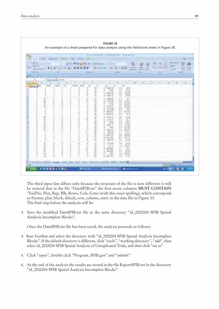
Data analysis 61
The third input line differs only because the structure of the file is now different: it will be noticed that in the file “DataSPIB.txt” the first seven columns MUST CONTAIN ‘TrialNo, Plot, Rep, Blk, Rows, Cols, Geno (with this exact spelling), which correspond to Farmer, plot, block, sblock, row, column, entry in the data file in Figure 33.
The final step before the analysis will be:
3. Save the modified DataSPIB.txt file in the same directory “id_2002004 SPIB Spatial Analysis Incomplete Blocks”.
Once the DataSPIB.txt file has been saved, the analysis proceeds as follows:
4. Start GenStat and select the directory with “id_2002004 SPIB Spatial Analysis Incomplete Blocks”. If the default directory is different, click “tools”, “working directory”, “add”, then select id_2002004 SPIB Spatial Analysis of Unreplicated Trials, and then click “set as”.
5. Click “open”, double click “Program_SPIB.gen” and “submit”
6. At the end of the analysis the results are stored in the file ReportSPIB.txt in the directory “id_2002004 SPIB Spatial Analysis Incomplete Blocks”.
FIGURE 33An example of a sheet prepared for data analysis using the field book sheet in Figure 30.

Plant breeding with farmers – a technical manual62
UPDATING A FILE FOR DATA ANALYSIS: REPLICATED TRIALSIn this section we will discuss the case of replicated trials, such as those of Stage 4, with replications planted by different farmers (Figure 18), or trials of Stages 2 and 3 when, because of limited farm size, the trials have to be subdivided and therefore it is not possible to maintain the row and column structure.
The relevant columns for the analysis are shown in Figure 34, together with the variables to be analysed. It will be noticed that in this case we only need three columns to describe the data set, namely “Trial”, “Farmer” and “entry” because the programme takes farmers as “blocks” and the row sequence as the plot sequence. The other data, the variables, are as described in the previous cases.
SPATIAL ANALYSIS OF A REPLICATED TRIALSOnce the data are prepared as in Figure 34, it is possible to proceed to the analysis following the steps below:
1. Open the directory “id_2002001 RCBD (randomized complete block design”.
2. Open the file “DataRCBD.txt”. As in the previous cases the first part of the file is simply a set of instructions followed by the input lines, which in this case are only three as the one about the spatial models is not included.
Therefore the three input lines correspond to the second, third and fourth input lines described in the case of the unreplicated and replicated trials in rows and columns.
After pasting the data from the sheet shown in Figure 34 the file “DataRCBD.txt” looks like below:
FIGURE 34An example of a sheet prepared for data analysis
using the field book sheet in Figure 31.

Data analysis 63
21 1 8 42 5 1216.666667 3.666666667 32.5
21 1 2 52 8 1268.75 3.666666667 29.41666667
21 1 6 37 5 1345.833333 3.666666667 38.33333333
21 1 4 45 8 1416.666667 4 31.58333333
21 1 7 32 5 1095.833333 3 34.33333333
21 1 5 31 4 908.3333333 3 32.2
21 1 3 39 6 1258.333333 4 31.95
21 1 9 43 5 1570.833333 4 35.33333333
21 1 1 41 7 1081.25 3.333333333 29.41666667
21 2 7 28 5 900 2 34.18333333
21 2 1 41 5 1035.416667 2.666666667 30.06666667
21 2 6 29 4 1131.25 2.666666667 36.93333333
21 2 9 32 6 1081.25 2.666666667 35.08333333
21 2 3 35 5 1143.75 3.333333333 33.25
21 2 4 37 8 1197.916667 4 33.68333333
21 2 2 46 8 1145.833333 3.333333333 28.81666667
21 2 8 32 7 954.1666667 3 31.86666667
21 2 5 27 3 789.5833333 1.333333333 33.06666667
After saving the file without changing the name, the analysis proceeds as follows:
3. Start GenStat and select the directory with “id_2002001 RCBD (randomized complete block design”. If the default directory is different, click “tools”, “working directory”, “add”, then select “id_2002001 RCBD (randomized complete block design”, and click “set as”.
4. Click “open”, double click “Prog RCBD.gen” and “submit”
5. At the end of the analysis the results are stored in two files: ReportRCBDmeans.txt with the means and statistical parameters, and ReportRCBDAnovas.txt with the analysis of variance for each variable.
DATA ANALYSIS OF A REPLICATED TRIALS WITH ALPHANALThe software ALPHANAL introduced in the section on randomization can also be used for the analysis of replicated trials regardless of whether the incomplete blocks and/or the replications are physically adjacent to each other.
In this case, open the directory ALPHANAL and click ALPHANAL.exe. The programme starts by asking the “plan file name” (Figure 35), i.e. the name of the randomization file that has been stored at the time it was generated.
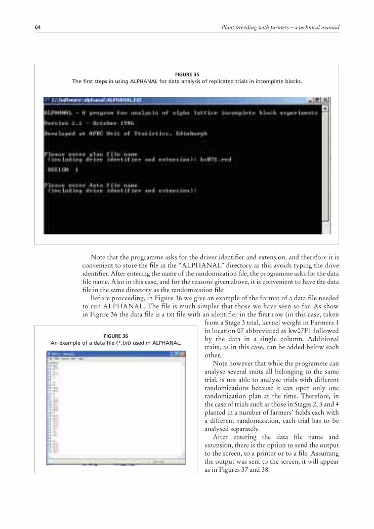
Plant breeding with farmers – a technical manual64
FIGURE 35The first steps in using ALPHANAL for data analysis of replicated trials in incomplete blocks.
FIGURE 36An example of a data file (*.txt) used in ALPHANAL.
Note that the programme asks for the driver identifier and extension, and therefore it is convenient to store the file in the “ALPHANAL” directory as this avoids typing the drive identifier. After entering the name of the randomization file, the programme asks for the data file name. Also in this case, and for the reasons given above, it is convenient to have the data file in the same directory as the randomization file.
Before proceeding, in Figure 36 we give an example of the format of a data file needed to run ALPHANAL. The file is much simpler that those we have seen so far. As show in Figure 36 the data file is a txt file with an identifier in the first row (in this case, taken
from a Stage 3 trial, kernel weight in Farmers 1 in location 07 abbreviated as kw07F1 followed by the data in a single column. Additional traits, as in this case, can be added below each other.
Note however that while the programme can analyse several traits all belonging to the same trial, is not able to analyse trials with different randomizations because it can open only one randomization plan at the time. Therefore, in the case of trials such as those in Stages 2, 3 and 4 planted in a number of farmers’ fields each with a different randomization, each trial has to be analysed separately.
After entering the data file name and extension, there is the option to send the output to the screen, to a printer or to a file. Assuming the output was sent to the screen, it will appear as in Figures 37 and 38.

Data analysis 65
The first part of the output (Figure 37) describes the structure of data using the information from the randomization file, the levels of the various factors (in this case replications, incomplete blocks and treatment (= entries), followed by the variable name and the raw data.
In the second part of the output (Figure 38) the adjusted means and their ranks are listed by entry number together with the mean of the original values and the original data.
This is followed by the standard statistics and the analysis of variance. Where the data file contains more variables, the outputs for the various variables appear one after the other.
Importing the results of the analysisThe results of the analysis of unreplicated trials and of the replicated trials in rows and columns are stored, as already mentioned, in the files ReportSPUR.txt and ReportSPIB.txt in their respective directories.
The two files have a very similar structure and will be described together, underlining the differences between them.
The two files have a header including the date and the time of the analysis:
FIGURE 37The first part of the output file of the analysis of incomplete block conducted with ALPHANAL.

Plant breeding with farmers – a technical manual66
This is followed by a description of the file which has just been analysed. Here it has to be noted that the program has been designed to analyse a series of trials with similar structure and this is the reason for the presence of the column “trial”.
This section in the case of the ReportSPUR.txt is as follows:
FIGURE 38The second (and last) part of the output file of the analysis of incomplete block conducted
with ALPHANAL.
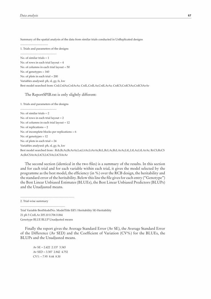
Data analysis 67
The ReportSPIB.txt is only slightly different:
The second section (identical in the two files) is a summary of the results. In this section and for each trial and for each variable within each trial, it gives the model selected by the programme as the best model, the efficiency (in %) over the RCB design, the heritability and the standard error of the heritability. Below this line the file gives for each entry (“Genotype”) the Best Linear Unbiased Estimates (BLUEs), the Best Linear Unbiased Predictors (BLUPs) and the Unadjusted means.
Finally the report gives the Average Standard Error (Av SE), the Average Standard Error of the Difference (Av SED) and the Coefficient of Variation (CV%) for the BLUEs, the BLUPs and the Unadjusted means.
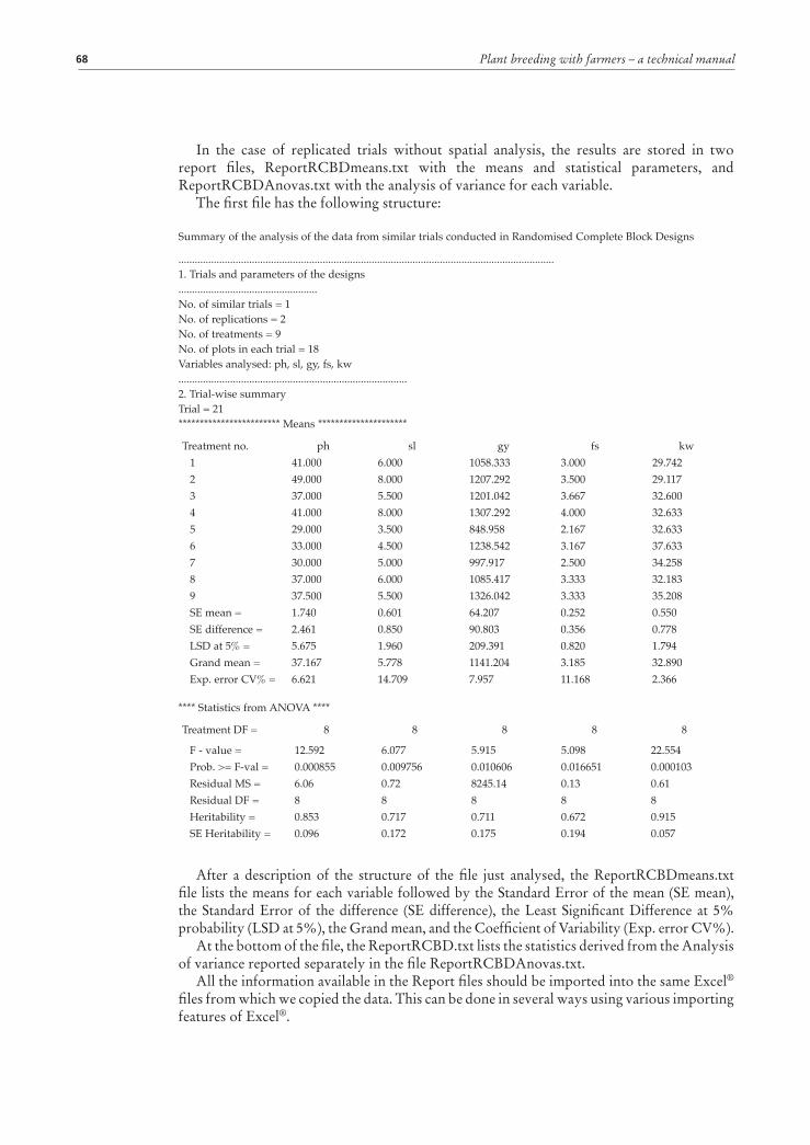
Plant breeding with farmers – a technical manual68
In the case of replicated trials without spatial analysis, the results are stored in two report files, ReportRCBDmeans.txt with the means and statistical parameters, and ReportRCBDAnovas.txt with the analysis of variance for each variable.
The first file has the following structure:
After a description of the structure of the file just analysed, the ReportRCBDmeans.txt file lists the means for each variable followed by the Standard Error of the mean (SE mean), the Standard Error of the difference (SE difference), the Least Significant Difference at 5% probability (LSD at 5%), the Grand mean, and the Coefficient of Variability (Exp. error CV%).
At the bottom of the file, the ReportRCBD.txt lists the statistics derived from the Analysis of variance reported separately in the file ReportRCBDAnovas.txt.
All the information available in the Report files should be imported into the same Excel® files from which we copied the data. This can be done in several ways using various importing features of Excel®.
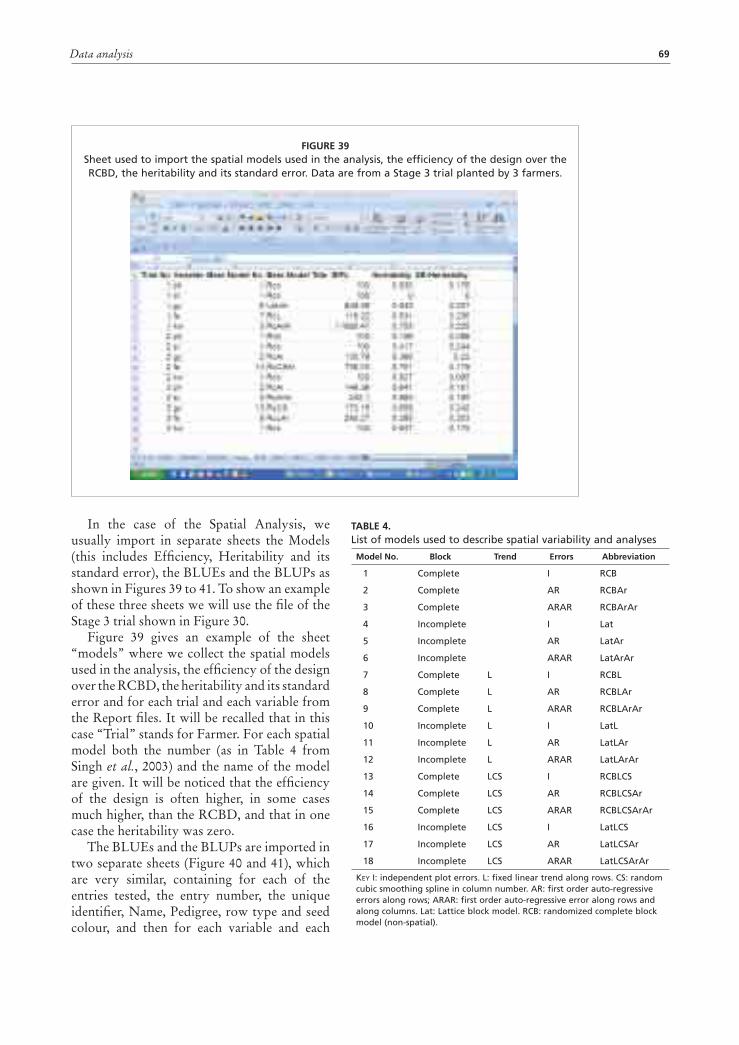
Data analysis 69
In the case of the Spatial Analysis, we usually import in separate sheets the Models (this includes Efficiency, Heritability and its standard error), the BLUEs and the BLUPs as shown in Figures 39 to 41. To show an example of these three sheets we will use the file of the Stage 3 trial shown in Figure 30.
Figure 39 gives an example of the sheet “models” where we collect the spatial models used in the analysis, the efficiency of the design over the RCBD, the heritability and its standard error and for each trial and each variable from the Report files. It will be recalled that in this case “Trial” stands for Farmer. For each spatial model both the number (as in Table 4 from Singh et al., 2003) and the name of the model are given. It will be noticed that the efficiency of the design is often higher, in some cases much higher, than the RCBD, and that in one case the heritability was zero.
The BLUEs and the BLUPs are imported in two separate sheets (Figure 40 and 41), which are very similar, containing for each of the entries tested, the entry number, the unique identifier, Name, Pedigree, row type and seed colour, and then for each variable and each
FIGURE 39Sheet used to import the spatial models used in the analysis, the efficiency of the design over the RCBD, the heritability and its standard error. Data are from a Stage 3 trial planted by 3 farmers.
TABLE 4. List of models used to describe spatial variability and analyses
Model No. Block Trend Errors Abbreviation
1 Complete I RCB
2 Complete AR RCBAr
3 Complete ARAR RCBArAr
4 Incomplete I Lat
5 Incomplete AR LatAr
6 Incomplete ARAR LatArAr
7 Complete L I RCBL
8 Complete L AR RCBLAr
9 Complete L ARAR RCBLArAr
10 Incomplete L I LatL
11 Incomplete L AR LatLAr
12 Incomplete L ARAR LatLArAr
13 Complete LCS I RCBLCS
14 Complete LCS AR RCBLCSAr
15 Complete LCS ARAR RCBLCSArAr
16 Incomplete LCS I LatLCS
17 Incomplete LCS AR LatLCSAr
18 Incomplete LCS ARAR LatLCSArAr
KEY I: independent plot errors. L: fixed linear trend along rows. CS: random cubic smoothing spline in column number. AR: first order auto-regressive errors along rows; ARAR: first order auto-regressive error along rows and along columns. Lat: Lattice block model. RCB: randomized complete block model (non-spatial).

Plant breeding with farmers – a technical manual70
FIGURE 40An example of a sheet used to import the Best Linear Unbiased Estimates (BLUEs) of the genotypic values of
the entries tested in a Stage 3 trial grown by 3 farmers.
FIGURE 41An example of a sheet used to import the Best Linear Unbiased Predictors (BLUPs) of the
genotypic values of the entries tested in a Stage 3 trial grown by 3 farmers.

Data analysis 71
farmer, the respective BLUEs and BLUPs. In both cases the bottom rows of the sheets show mean, minimum and maximum, the Average Standard Error (Av SE), the Average Standard Error of the Difference (Av SED) and the Coefficient of Variation (CV %). These statistics can be used to statistically compare any two varieties.
In the case of Stage 1 trials, such as the one shown in Figure 20, the three sheets (Models, BLUEs and BLUPs) will be the same as described above, with the difference that in the sheet “Models” the column Trial indicate the village and that in the sheets “BLUEs” and “BLUPs” there will be only one value for each genotype and each variable as the trial is usually grown by only one farmer.
Eventually, in the case of the trials in which the replications are planted by different farmers, the full report as shown in page 68 is imported as such in one sheet of the Excel® file. The same applies for the output files produced by ALPHANAL.
DISCUSSION OF RESULTS AND FARMERS’ FINAL SELECTIONTogether with the visual selection in the field, the farmers’ final selection is a key activity in a PPB programme. It is therefore important to prepare tables which summarize the results in such a transparent way as to make it possible for the farmers to decide which entries to select and which entries to discard. These tables differ in the different stages of the PPB programme because the amounts of information available increases as the entries move from one stage to the next, as we will see later.
Stage 1 trialsThe first step in summarizing the results of a Stage 1 PPB trial for discussion with farmers is to import the BLUPs in a new sheet ("Table 1” shown in Figure 42) and then, using the command “rank and percentile” under “Data analysis” in Excel®1, to rank each variable either in ascending or descending order depending on the variable (for example for variables such as those in the file shown in Figure 42 the descending order is the most appropriate but in the case of variables such as heading, maturity and disease susceptibility, the ascending order may be more appropriate if earliness and resistance are the desirable attributes). The ranks are added in the file to the right of the respective variable, and are important because they allow farmers to select based on the relative rather than the absolute values.
When the number of entries is large, as in this case, farmers in a number of countries have expressed the desire of facilitating their inspection of the data by preparing two additional summary tables: one with approximately the best 10–15% entries for grain yield and the second with the best 10–15% entries for farmers’ score. Examples of these tables are shown in Figures 43 and 44 for a Stage 1 trial with 160 entries.
The advantage of these tables is that they allow farmers to evaluate the entries not only for the character for which they excel (grain yield and farmers’ score, respectively) but also for all the other characters that have been measured.
The tables shown in Figures 43 and 44 also allow farmers to check immediately how precise their visual selection was in identifying the highest yielding entries: the two tables have 4 entries in common (100, 121, 10 and 9) which were therefore among the best 12.5% for both grain yield and farmers’ score. It is also very useful to have in these tables those varieties that farmers know well regardless of their ranking.
The summary tables are not strictly needed and should be prepared only if requested by farmers as has happened in the PPB programmes in some countries.
Once the three tables have been prepared they need to be translated in the language(s) familiar to the farmers so that they can use them without any external assistance. In the translation is useful to keep the number of decimals to the bare minimum.
1 Available as one of the “Add ins” under “Excel Options”

Plant breeding with farmers – a technical manual72
During the meeting in which the farmers will eventually make the final selections, the researchers should not interfere in the discussion, should avoid any influence on the decisions that are taken, should make sure that the discussion is as smooth as possible and should resolve conflicts in those cases where the farmers can not reach a consensus. As the PPB programme progresses it is not unusual that, at least in some villages, some farmers develop the ability to lead these discussions, which then become flexible in terms of timing, and certainly become completely independent from any influence of the scientists. It is not within the scope of this manual to analyse the selection criteria used by the farmers, but to show how to properly record the decisions of the farmers. If the selection is made using tables such as those in Figures 43 and 44, the selection of the farmers can be recorded by adding a column of “1” (selected) and “0” (unselected) (Figures 45 and 46).
It will be noticed that (1) the highest yielding entries are not always selected by farmers, and (2) the 4 entries among the best 12.5% for both grain yield and farmers’ score were selected in both tables. The final steps, after the farmers’ selection is concluded, are:
1. Transfer the data from column R of sheet “Tables 2” and “Table 3” into column R of sheet Table 1.
2. Sort the sheet “Table 1” for descending order of column R and for ascending order of column B.
The result is shown in Figure 47, with the 17 entries selected by farmers and the three checks (highlighted). These were added because two are PPB varieties already adopted by farmers and one is the popular landrace grown in the area.
FIGURE 42The first step of preparing the data for meeting the farmers and discuss the results of a Stage 1 of a PPB trial is
to copy the BLUPs in a new sheet “Table 1” and rank them.
Data analysis 73
FIGURE 43The 20 highest yielding entries in a Stage 1 trial with 160 entries shown in Figure 42 together with a number of
reference varieties (rows 23 – 28), i.e. varieties known or released or already adopted by farmers.
FIGURE 44 The 20 entries with the highest average farmers’ score together with a number of reference varieties (rows 23-31),
i.e. varieties known or released or already adopted by farmers.

Plant breeding with farmers – a technical manual74
FIGURE 45Figure 43 after farmers’ selection, with the additional column “ST 2” (for Stage 2) showing the selected (1)
and the discarded entries (0).
FIGURE 46 Figure 44 after farmers’ selection, with the additional column “ST 2” showing the selected (1) and the
discarded entries (0).
Data analysis 75
The sheet shown in Figure 47 becomes, after few modifications, the first sheet “entries” of the Stage 2 trial to be planted by a given number of farmers in the following year (Figure 48).
The comparison between Figures 47 and 48 shows that the only modifications are the replacement of the old column “Entry” with a new one from 1 to 20, and the addition of a new identification number for Stage 2 trials in the current cropping season.
The randomization and the preparation of the “fieldbook” sheet will be the first steps to prepare for the planting of the Stage 2 trials with the entries selected by the farmers.
Stage 2 trialsAfter having seen the entire process, from the preparation of the tables for discussion with farmers, to the farmers’ selection in a Stage 1 trial and the building of the new file for Stage 2 trials, it should be easier to understand that when the same process is applied to the data of Stage 2 trials there will be two main differences:
• Data will be available from more than one farmer.• Data will be available from two years (the Stage 1 grown in the previous year and
Stage 2 grown in the current year).These differences do not affect the first step, which is to copy the BLUPs into a sheet
called “Table 1” (Figure 49), which differs from the “Table 1” we have seen in the case of the Stage 1 trial because now for each variable we have a value for each farmer (in this case, three farmers).
Before deciding how to finalize the table for the farmers’ selection it is necessary to discuss with the farmers whether they prefer to select on the basis of the results obtained in each farmers’ field or on the basis of the means across farmers.
In the first case it will be necessary to rank the entries (as shown in the case of "Table 1" in Figure 42) farmer by farmer, prepare one table for each farmer, and proceed as in the case
FIGURE 47The list of the 17 entries promoted from Stage 1 to Stage 2 plus three checks (highlighted and bold).

Plant breeding with farmers – a technical manual76
FIGURE 48The new file with the entries promoted from Stage 1 to Stage 2, with the “fldbook” sheet and the randomization
plan “RND” (not shown).
FIGURE 49 The structure of the sheet “Table 1” in the case of a Stage 2 trial with 20 entries grown by three farmers.
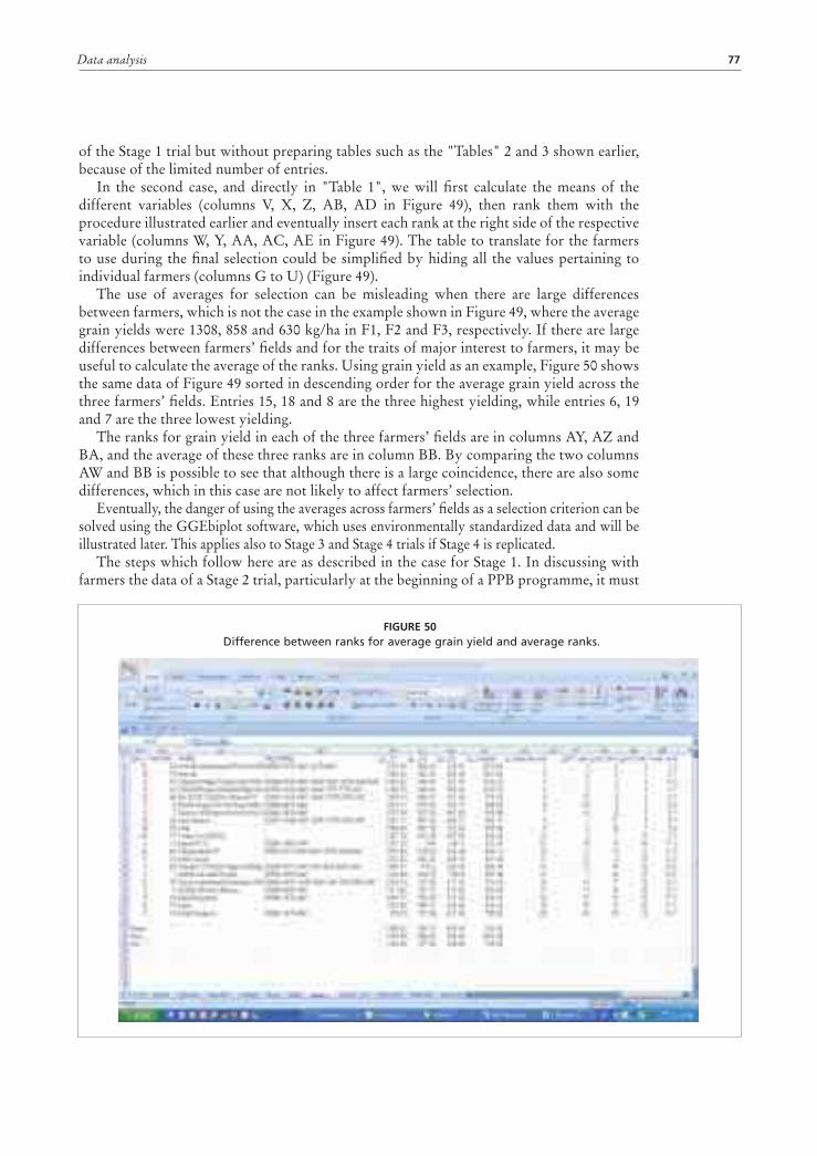
Data analysis 77
of the Stage 1 trial but without preparing tables such as the "Tables" 2 and 3 shown earlier, because of the limited number of entries.
In the second case, and directly in "Table 1", we will first calculate the means of the different variables (columns V, X, Z, AB, AD in Figure 49), then rank them with the procedure illustrated earlier and eventually insert each rank at the right side of the respective variable (columns W, Y, AA, AC, AE in Figure 49). The table to translate for the farmers to use during the final selection could be simplified by hiding all the values pertaining to individual farmers (columns G to U) (Figure 49).
The use of averages for selection can be misleading when there are large differences between farmers, which is not the case in the example shown in Figure 49, where the average grain yields were 1308, 858 and 630 kg/ha in F1, F2 and F3, respectively. If there are large differences between farmers’ fields and for the traits of major interest to farmers, it may be useful to calculate the average of the ranks. Using grain yield as an example, Figure 50 shows the same data of Figure 49 sorted in descending order for the average grain yield across the three farmers’ fields. Entries 15, 18 and 8 are the three highest yielding, while entries 6, 19 and 7 are the three lowest yielding.
The ranks for grain yield in each of the three farmers’ fields are in columns AY, AZ and BA, and the average of these three ranks are in column BB. By comparing the two columns AW and BB is possible to see that although there is a large coincidence, there are also some differences, which in this case are not likely to affect farmers’ selection.
Eventually, the danger of using the averages across farmers’ fields as a selection criterion can be solved using the GGEbiplot software, which uses environmentally standardized data and will be illustrated later. This applies also to Stage 3 and Stage 4 trials if Stage 4 is replicated.
The steps which follow here are as described in the case for Stage 1. In discussing with farmers the data of a Stage 2 trial, particularly at the beginning of a PPB programme, it must
FIGURE 50 Difference between ranks for average grain yield and average ranks.

Plant breeding with farmers – a technical manual78
be made clear to them that in addition to the choice among selecting on the basis of the performance in individual farmers’ fields or on the basis of the average performance across farmers’ fields, another choice is between selecting on the basis on the data of the Stage 2 results only, or on the basis of the combined data of Stages 1 and 2. Our experience is that, when the farmers are offered this choice, they prefer to use the combined data and to ignore individual year data. Continuing with our example, the combined data are shown in the sheet “Table 2 (2Y)” (Figure 51) which contains all the data collected in Stage 1 (conducted the year before) as well as all those collected in Stage 2. Figure 51 shows the BLUPs collected in the two years and on the right side (shown in Figure 52) the means over the two years (the two figures are actually the same sheet, which has too many columns to fit in one figure).
Farmers’ selections are entered in the usual way (1 = selected and 0 = discarded) in the far right column (AQ) name “ST 3” (= promoted to Stage 3) (Figure 52), the sheet is sorted for this column in descending order and for entry number in ascending order and the resulting file (Figure 53) shows (highlighted) the 9 entries selected to be tested in Stage 3 trials in the following year.
As in the case of the Stage 2 trial, the highlighted portion of the sheet “Table 2 (2Y)” of Figure 53 becomes the sheet “entries” of the Stage 3 trial to be planted by a given number of farmers in the following year after replacing the old column “Entry” with a new one and after adding a new identification number for Stage 3 trials in the current cropping season. The randomization and the preparation of the “fieldbook” sheet will be the first steps to prepare the planting of the Stage 3 trials with the entries selected by the farmers.
Stage 3 trialsThe process as illustrated for the Stage 2 trials applies to Stage 3 trials, with the difference that the amount of information available to farmers will be larger and the number of lines fewer. In the case of Stage 3 trials, the farmers will have the choice between (1) selection based on the performance in individual farmers' fields in the current cropping season; (2) selection based on the average performance across farmers fields in the current cropping season; or (3) selection based on the combined performance in Stage 1, Stage 2 and Stage 3 trials, namely on 3 years of data.
The first step is to copy the BLUPs into a sheet called “Table 1” (Figure 54), which differs from the “Table 1” we have seen in the case of the Stage 2 trial only because of fewer lines.
As shown in Figure 55, in a Stage 3 trial we have data from three years, namely the Stage 1 trial conducted 2 years earlier, Stage 2 conducted the year before, and Stage 3 conducted in the current year (the data are actually aligned side by side, as in Figure 51 and not as shown in Figure 55.
Two points are worth noting in Figure 55. Firstly, the danger of adding reference varieties or new checks during the course of the same breeding cycle. Entries 6 and 12, which were not included in Stage 1 and Stage 2, were added only in Stage 3. In such a case we can use the new entries as reference for the performance in Stage 3 but not as a reference to judge the performance across the three cropping seasons, particularly if the means of grain yield and other data of the three years are substantially different. The second point is that of always using the same sequence when entering the variables in a file. For example, if the variables ph, sl, fs, kw and gy were entered in this sequence in Stage 1, it is very useful to keep the same sequence in Stages 2, 3 and 4 because this will make it much easier to calculate the means across stages with the Excel® function “Average”.
These are reported in Figure 56, together with their rank and the farmers’ final selection in column BG (ST 4). It will be noticed that only 5 of the original 160 entries (entries 3, 4, 5, 7 and 8) have reached the final stage of evaluation. The other entries in the file are checks.

Data analysis 79
FIG
UR
E 51
A s
um
mar
y o
f th
e 2
year
s d
ata
colle
cted
in S
tag
e 1
and
Sta
ge
2 tr
ials
. Tab
le 2
(2Y
) co
nti
nu
es in
Fig
ure
52.
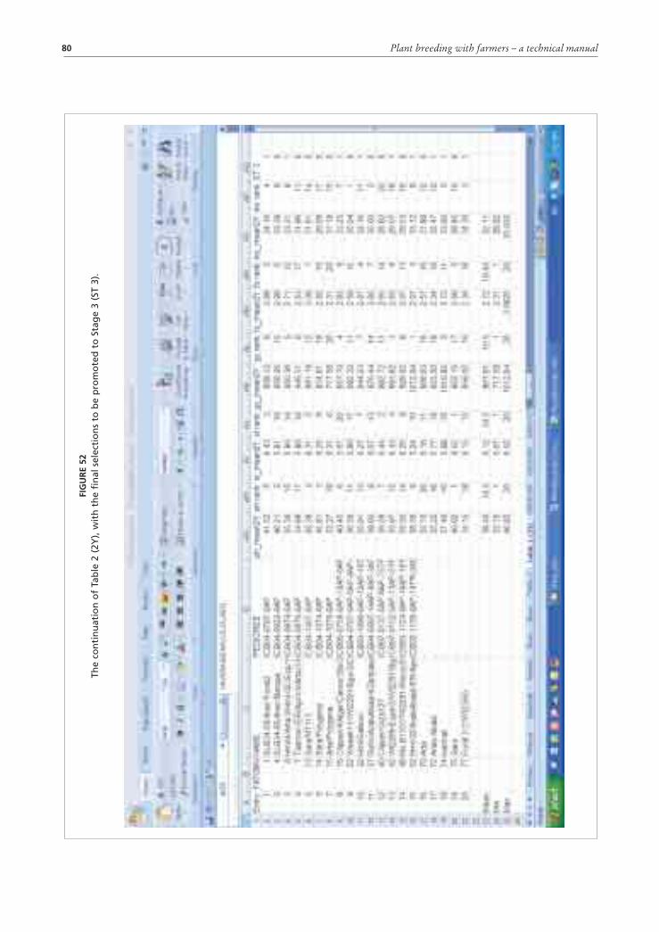
Plant breeding with farmers – a technical manual80
FIG
UR
E 52
The
con
tin
uat
ion
of
Tab
le 2
(2Y
), w
ith
th
e fi
nal
sel
ecti
on
s to
be
pro
mo
ted
to
Sta
ge
3 (S
T 3)
.

Data analysis 81
FIGURE 53The second part of Table 2 (2Y) sorted for the entries promoted to Stage 3 (ST 3).
FIGURE 54The structure of the sheet “Table 1” in the case of a Stage 3 trial with 12 entries grown by three farmers.
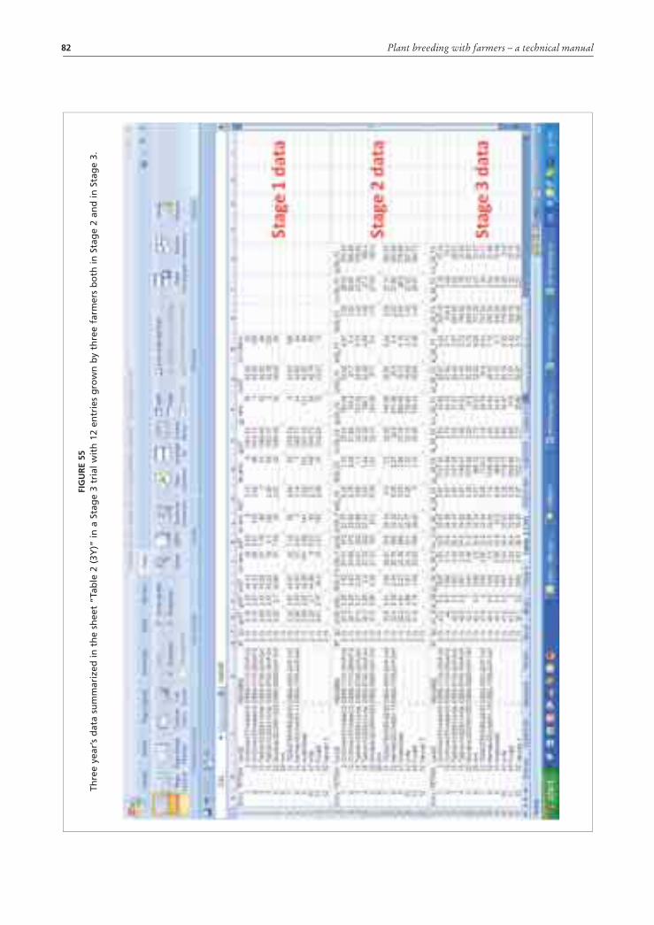
Plant breeding with farmers – a technical manual82
FIG
UR
E 55
Thre
e ye
ar’s
dat
a su
mm
ariz
ed in
th
e sh
eet
“Tab
le 2
(3Y
)” in
a S
tag
e 3
tria
l wit
h 1
2 en
trie
s g
row
n b
y th
ree
farm
ers
bo
th in
Sta
ge
2 an
d in
Sta
ge
3.
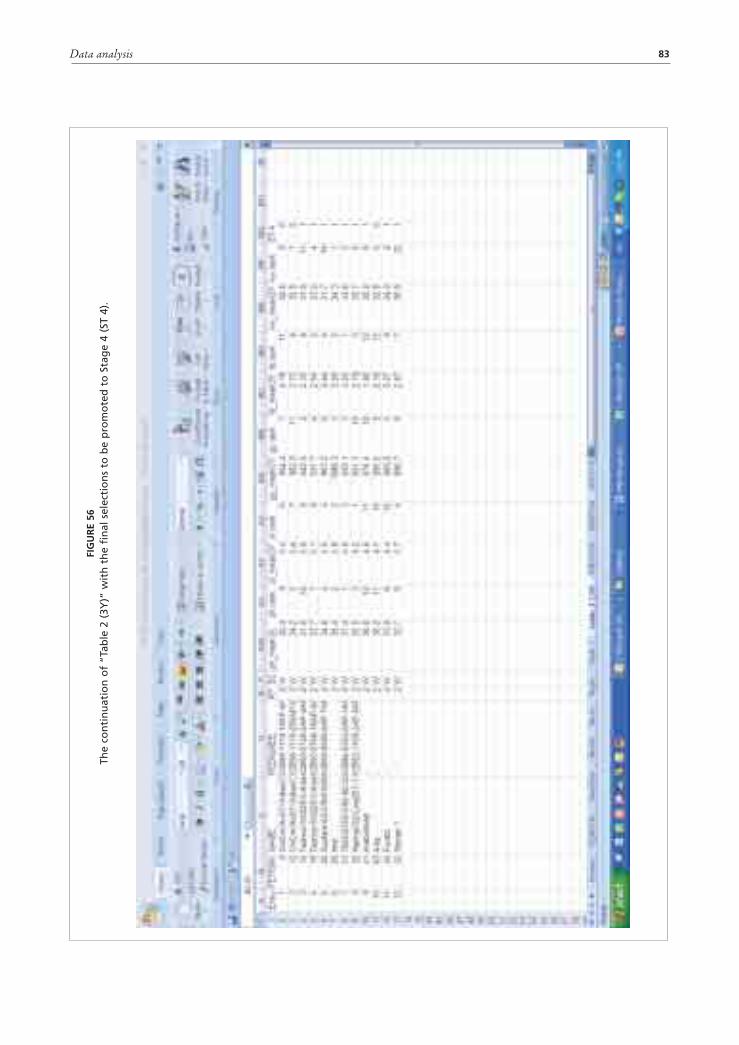
Data analysis 83
FIG
UR
E 56
The
con
tin
uat
ion
of
“Tab
le 2
(3Y
)” w
ith
th
e fi
nal
sel
ecti
on
s to
be
pro
mo
ted
to
Sta
ge
4 (S
T 4)
.
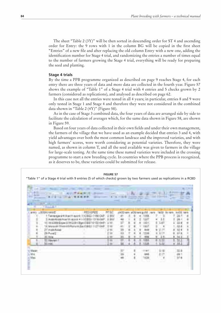
Plant breeding with farmers – a technical manual84
The sheet “Table 2 (3Y)” will be then sorted in descending order for ST 4 and ascending order for Entry: the 9 rows with 1 in the column BG will be copied in the first sheet “Entries” of a new file and after replacing the old column Entry with a new one, adding the identification number for Stage 4 trial, and randomizing the entries a number of times equal to the number of farmers growing the Stage 4 trial, everything will be ready for preparing the seed and planting.
Stage 4 trialsBy the time a PPB programme organized as described on page 9 reaches Stage 4, for each entry there are three years of data and more data are collected in the fourth year. Figure 57 shows the example of “Table 1” of a Stage 4 trial with 4 entries and 5 checks grown by 2 farmers (considered as replications), and analysed as described on page 62.
In this case not all the entries were tested in all 4 years; in particular, entries 8 and 9 were only tested in Stage 1 and Stage 4 and therefore they were not considered in the combined data shown in “Table 2 (4Y)” (Figure 58).
As in the case of Stage 3 combined data, the four years of data are arranged side by side to facilitate the calculation of averages which, for the same data shown in Figure 58, are shown in Figure 59.
Based on four years of data collected in their own fields and under their own management, the farmers of the village that we have used as an example decided that entries 3 and 4, with yield advantages over both the most common landrace and the improved varieties, and with high farmers’ scores, were worth considering as potential varieties. Therefore, they were named, as shown in column T, and all the seed available was given to farmers in the village for large-scale testing. At the same time these named varieties were included in the crossing programme to start a new breeding cycle. In countries where the PPB process is recognized, as it deserves to be, these varieties could be submitted for release.
FIGURE 57“Table 1” of a Stage 4 trial with 9 entries (5 of which checks) grown by two farmers used as replications in a RCBD
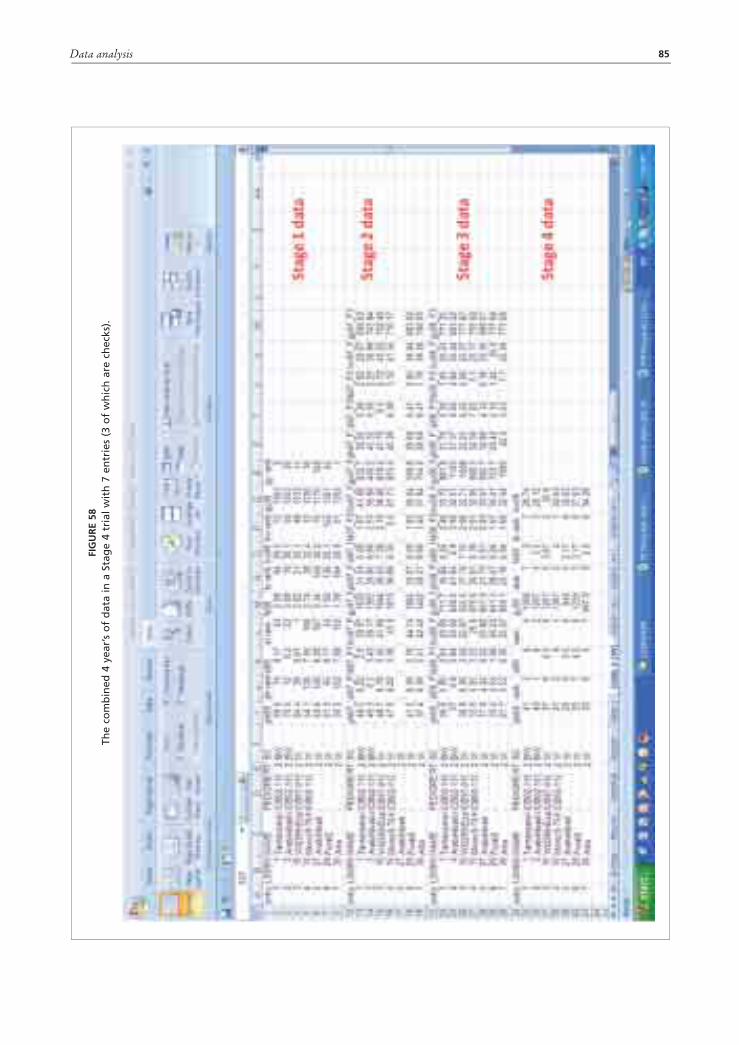
Data analysis 85
FIG
UR
E 58
The
com
bin
ed 4
yea
r’s
of
dat
a in
a S
tag
e 4
tria
l wit
h 7
en
trie
s (3
of
wh
ich
are
ch
ecks
).

Plant breeding with farmers – a technical manual86
One of the advantages of the system of file keeping that we have shown is that the data needed for the preparation of the report to submit to the variety release committee are ready within the Stage 4 file.
Whether they are released or not, it is important to ensure that these varieties are accessible to all and that the benefits deriving from their use is shared among all those who have contributed to their development.
GENOTYPE × ENVIRONMENT INTERACTIONS Plant breeding, whether participatory or not, is a complex process and in the majority of cases (the only notable exception being the breeding programmes in Australia), only a small fraction of it takes place in farmers’ fields. Usually most of the process takes place on one or more research stations, and all the decisions are made by the breeders and collaborating scientists (pathologists, entomologists, quality specialists, etc.).
Studies conducted in Australia (Pederson and Rathjen, 1981; Cooper et al., 1997) to evaluate the relevance of research stations for their suitability as selection environments have found that, in many cases, the genetic correlations between the yield of breeding lines on the research station and yield under on-farm conditions were low in comparison with the genetic correlations between different on-farm experiments. Therefore, while lower experimental errors and higher heritability could be achieved on the research stations, the results were found to have limited relevance to genotype performance in the on-farm target population of environments. Consequently, there was an investment into capability for conducting large breeding trials under on-farm conditions at all stages of the breeding
FIGURE 59 Four year’s means and two entries selected and named by farmers as potential varieties at the end
of a breeding cycle.

Data analysis 87
programme in order to increase the chances of conducting Multi-Environment Trials (METs) across years and locations, that were accurately targeted to the farming systems (Bänziger and Cooper, 2001).
One of the main consequences of the low correlation between the yield of breeding lines on the research station and yield under on-farm conditions is that a large amount of breeding material might be discarded before knowing whether it could have been useful in the real conditions of farmers’ fields, and the one selected is likely to perform well in environments similar to that of the research stations, but not in environments that are very different. This is because of Genotype × Environment (G×E) interactions, which are one of the major factors limiting the efficiency of breeding programmes when they cause a change of ranking between genotypes in different environments (cross-over or qualitative interactions).
In statistical terms, it is regarded as no G×E interaction when the difference between, for example, two varieties A and B (Figure 60) remains constant regardless whether the comparison is conducted in one location or year (E1) or in another (E2). When the difference changes, as shown in Figure 61, there is a quantitative type of G×E interaction. These types of interactions are not a problem to a breeder because, regardless of where or how the comparison between varieties is conducted, variety A is always superior to variety B and therefore there will be no doubts as to which variety to select. The problem for the breeder is when the G×E interactions are of qualitative
FIGURE 60Absence of G×E interactions (left with Δ = Δ’) and quantitative type of G×E interactions (right with Δ ≠ Δ’
but of the same sign).
FIGURE 61 Qualitative (cross-over) type of G×E interactions with Δ
and Δ’ of opposite sign.

Plant breeding with farmers – a technical manual88
(cross-over) type, because in this case the decision of which variety (A or B) is the best depends on where the comparison is conducted (Figure 61).
In general, when different lines or cultivars of a given crop are evaluated in a sufficiently wide range of environments, G×E interactions of cross-over type seem to be very common (Ceccarelli et al., 2001). We have argued (Ceccarelli, 1989) that for crops grown in environments poorly represented by the research stations this often results in useful breeding materials being discarded.
When G×E interactions are present the plant breeder can ignore them, avoid them or exploit them (Eisemann, Cooper and Woodruff, 1990). When G×E interactions are significantly large, it is not possible to ignore them and the two remaining strategies are (1) to avoid them by selecting material that is broadly adapted to the entire range of target environments, or (2) to exploit them by selecting a range of material, each adapted to a specific environment (Ceccarelli, 1989). The choice is based on a separate analysis of the two components of G×E interactions, namely Genotype × Years (G×Y) and Genotype × Locations (G×L), the first of which is largely unpredictable, while the second, if repeatable over time, identifies distinct target environments (Annicchiarico, Bellah and Chiari, 2005, 2006; Singh, Grando and Ceccarelli 2006).
A simple example of repeatable and unrepeatable G×L interactions is shown in Figures 62 and 63.
In both figures we show the results of a hypothetical trial conducted in two locations and in two years with seven genotypes. Both figures show the ranking for grain yield of the seven genotypes in each year×location combination. In Figure 62 the ranking of genotypes in year 1 changes substantially from location 1 (where genotypes 4 and 6 are the best and genotypes 5 and 7 the worse) to location 2 (where genotypes 7 and 2 are the best and genotypes 4 and
FIGURE 62An example of non-repeatable Genotype × Location (G×L) Interactions.
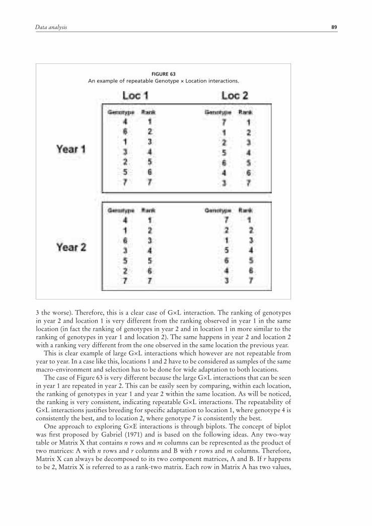
Data analysis 89
3 the worse). Therefore, this is a clear case of G×L interaction. The ranking of genotypes in year 2 and location 1 is very different from the ranking observed in year 1 in the same location (in fact the ranking of genotypes in year 2 and in location 1 in more similar to the ranking of genotypes in year 1 and location 2). The same happens in year 2 and location 2 with a ranking very different from the one observed in the same location the previous year.
This is clear example of large G×L interactions which however are not repeatable from year to year. In a case like this, locations 1 and 2 have to be considered as samples of the same macro-environment and selection has to be done for wide adaptation to both locations.
The case of Figure 63 is very different because the large G×L interactions that can be seen in year 1 are repeated in year 2. This can be easily seen by comparing, within each location, the ranking of genotypes in year 1 and year 2 within the same location. As will be noticed, the ranking is very consistent, indicating repeatable G×L interactions. The repeatability of G×L interactions justifies breeding for specific adaptation to location 1, where genotype 4 is consistently the best, and to location 2, where genotype 7 is consistently the best.
One approach to exploring G×E interactions is through biplots. The concept of biplot was first proposed by Gabriel (1971) and is based on the following ideas. Any two-way table or Matrix X that contains n rows and m columns can be represented as the product of two matrices: A with n rows and r columns and B with r rows and m columns. Therefore, Matrix X can always be decomposed to its two component matrices, A and B. If r happens to be 2, Matrix X is referred to as a rank-two matrix. Each row in Matrix A has two values,
FIGURE 63An example of repeatable Genotype × Location interactions.
Plant breeding with farmers – a technical manual90
which define a point in a two-dimensional plot. Similarly, each column in Matrix B has two values, which also define a point in a two-dimensional plot. The n rows of matrix A can be considered associated with n objects, e.g. n genotypes; similarly the m columns of matrix B can be considered associated with m environments. When both the n rows of A and m columns of B are displayed in a single plot, this plot is called a biplot. Therefore, the biplot of a rank-two matrix contains n + m points, compared with n × m values in the original matrix, and yet contains all of the matrix information (Yan, 2001).
The concept of GGE originates from analysis of METs of crop cultivars. The yield of a cultivar (or any other measure of cultivar performance) in an environment is a mixed effect of genotype main effect (G), environment main effect (E), and (G×E) interaction. In normal METs, E accounts for about 80% of the total yield variation, and G and G×E each account for about 10% (Gauch and Zobel, 1996; Yan et al., 2000). For the purpose of cultivar evaluation, however, only G and G×E are relevant (Gauch and Zobel, 1996). Furthermore, both G and G×E must be considered in cultivar evaluation, hence the term GGE (Yan et al., 2000). The analysis of GGEbiplot is now available in GenStat, but the graphics facilities are not as well developed as in the GGEbiplot software (www.ggebiplot.com) illustrated below.
GGEBIPLOT SOFTWARE The GGEbiplot software was developed to facilitate the use of the GGEbiplot analysis of MET data and other types of two-way data. GGEbiplot is graphical and interactive. It not only analyses the data and displays the GGEbiplot, but also allows the researcher to examine and address a number of key issues in the analysis of MET. In this section we will only cover some selected features of the GGEbiplot software. A list of references and the GGEbiplot web site will provide additional information.
Input data formatGGEbiplot is designed for the analysis of balanced two-way data with the genotypes (entries) as rows and the environments (testers) as columns. "Tester" is a generic term used in GGEbiplot to indicate locations, years, locations/years combinations and, as we will see later, traits. Data sets with missing cells can also be analysed.
GGEbiplot can read Excel® files as well as comma delimited files directly, and can use different types of input data format. The first and most common format is one in which each cell contains one observation. In this format the first column contains the entry number (header = entry) and all the other columns contain the data (for example grain yield) with the header in the first row.
In the case of PPB trials we suggest using the BLUPs obtained with one of the analyses described under Data Analysis and organized in a two-way table. In the specific case of PPB trials, the GGEbiplot can be conveniently used also to analyse associations between traits, and specifically between farmers’ scores and agronomic traits, and therefore to elucidate farmers’ selection criteria.
Missing cells, if any, need to be indicated with a unique symbol (for example *), they will be automatically replaced by the respective tester means, and the user will be notified of the number and the percentage of missing cells detected in the data set.
Other types of data sets that it is possible to analyse with the GGEbiplot software are:• Data in 4 columns (environments, replications, genotypes, values)• Data in 4 columns (environments, replications, genotypes and each trait)• Data in 5 columns (environments, replications, genotypes, trait and values) • Data in 5 columns (year, environments, replications, genotypes and each trait)• Data in 5 columns (year, environments, replications, genotypes, trait and values)• or any data format that is similar to that is used in SAS analysis.
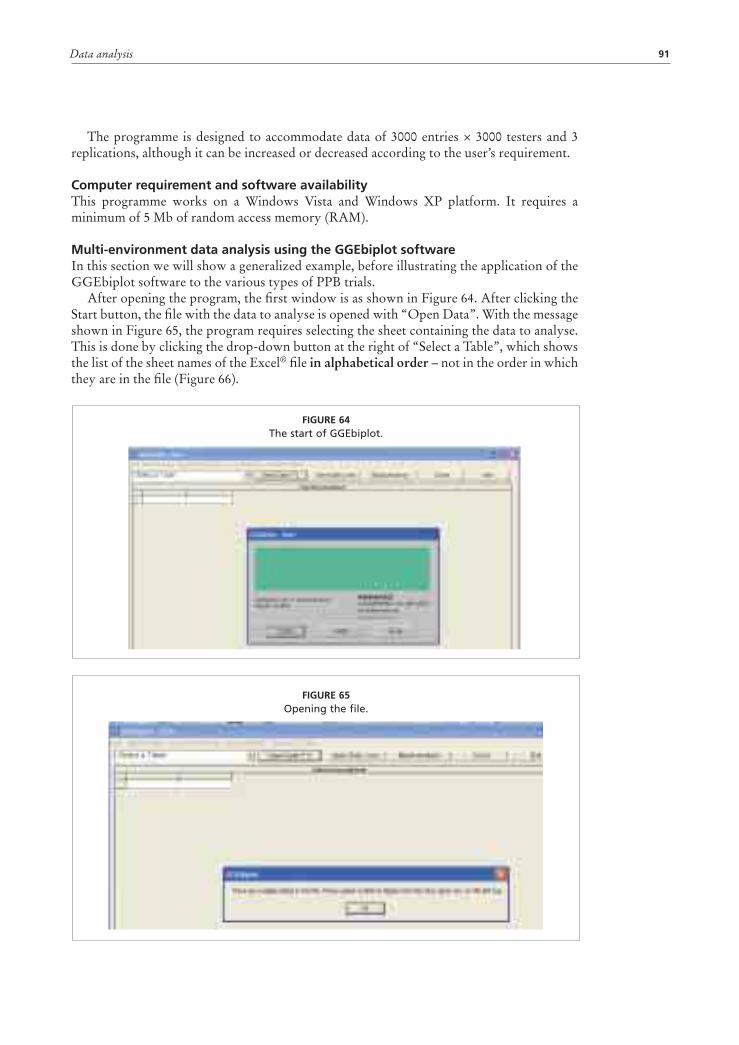
Data analysis 91
The programme is designed to accommodate data of 3000 entries × 3000 testers and 3 replications, although it can be increased or decreased according to the user’s requirement.
Computer requirement and software availabilityThis programme works on a Windows Vista and Windows XP platform. It requires a minimum of 5 Mb of random access memory (RAM).
Multi-environment data analysis using the GGEbiplot softwareIn this section we will show a generalized example, before illustrating the application of the GGEbiplot software to the various types of PPB trials.
After opening the program, the first window is as shown in Figure 64. After clicking the Start button, the file with the data to analyse is opened with “Open Data”. With the message shown in Figure 65, the program requires selecting the sheet containing the data to analyse. This is done by clicking the drop-down button at the right of “Select a Table”, which shows the list of the sheet names of the Excel® file in alphabetical order – not in the order in which they are in the file (Figure 66).
FIGURE 65Opening the file.
FIGURE 64The start of GGEbiplot.
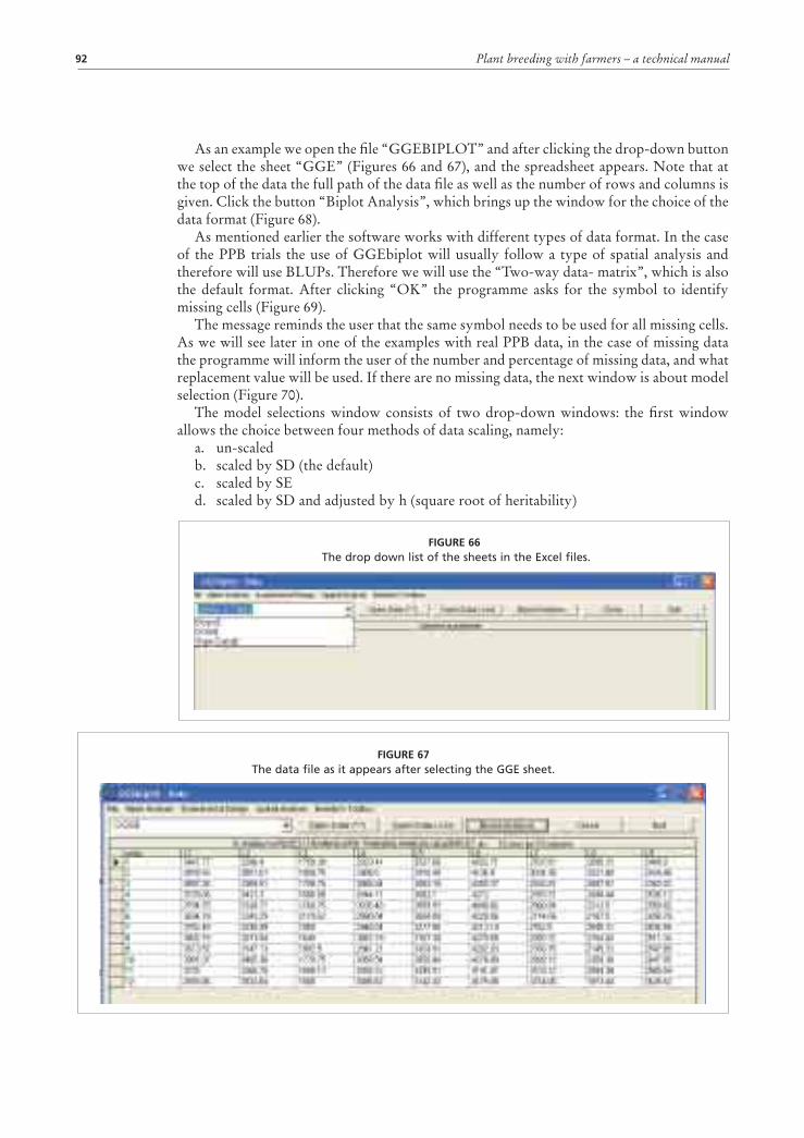
Plant breeding with farmers – a technical manual92
As an example we open the file “GGEBIPLOT” and after clicking the drop-down button we select the sheet “GGE” (Figures 66 and 67), and the spreadsheet appears. Note that at the top of the data the full path of the data file as well as the number of rows and columns is given. Click the button “Biplot Analysis”, which brings up the window for the choice of the data format (Figure 68).
As mentioned earlier the software works with different types of data format. In the case of the PPB trials the use of GGEbiplot will usually follow a type of spatial analysis and therefore will use BLUPs. Therefore we will use the “Two-way data- matrix”, which is also the default format. After clicking “OK” the programme asks for the symbol to identify missing cells (Figure 69).
The message reminds the user that the same symbol needs to be used for all missing cells. As we will see later in one of the examples with real PPB data, in the case of missing data the programme will inform the user of the number and percentage of missing data, and what replacement value will be used. If there are no missing data, the next window is about model selection (Figure 70).
The model selections window consists of two drop-down windows: the first window allows the choice between four methods of data scaling, namely:
a. un-scaledb. scaled by SD (the default)c. scaled by SEd. scaled by SD and adjusted by h (square root of heritability)
FIGURE 67The data file as it appears after selecting the GGE sheet.
FIGURE 66 The drop down list of the sheets in the Excel files.
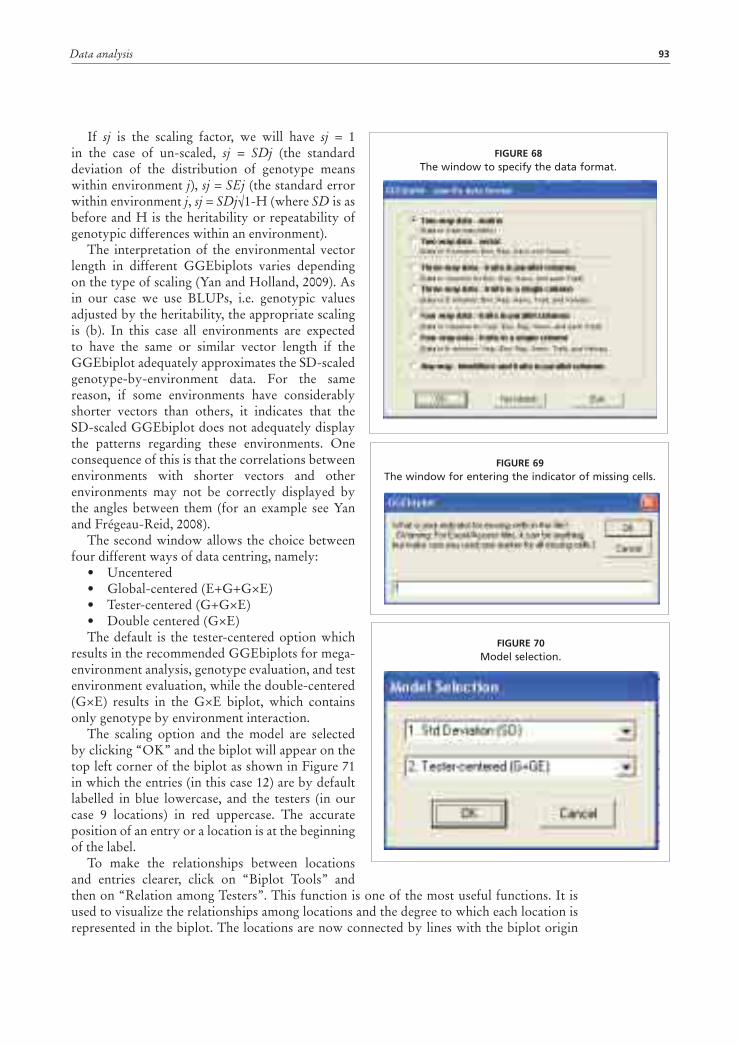
Data analysis 93
If sj is the scaling factor, we will have sj = 1 in the case of un-scaled, sj = SDj (the standard deviation of the distribution of genotype means within environment j), sj = SEj (the standard error within environment j, sj = SDj√1-H (where SD is as before and H is the heritability or repeatability of genotypic differences within an environment).
The interpretation of the environmental vector length in different GGEbiplots varies depending on the type of scaling (Yan and Holland, 2009). As in our case we use BLUPs, i.e. genotypic values adjusted by the heritability, the appropriate scaling is (b). In this case all environments are expected to have the same or similar vector length if the GGEbiplot adequately approximates the SD-scaled genotype-by-environment data. For the same reason, if some environments have considerably shorter vectors than others, it indicates that the SD-scaled GGEbiplot does not adequately display the patterns regarding these environments. One consequence of this is that the correlations between environments with shorter vectors and other environments may not be correctly displayed by the angles between them (for an example see Yan and Frégeau-Reid, 2008).
The second window allows the choice between four different ways of data centring, namely:
• Uncentered• Global-centered (E+G+G×E)• Tester-centered (G+G×E)• Double centered (G×E)The default is the tester-centered option which
results in the recommended GGEbiplots for mega-environment analysis, genotype evaluation, and test environment evaluation, while the double-centered (G×E) results in the G×E biplot, which contains only genotype by environment interaction.
The scaling option and the model are selected by clicking “OK” and the biplot will appear on the top left corner of the biplot as shown in Figure 71 in which the entries (in this case 12) are by default labelled in blue lowercase, and the testers (in our case 9 locations) in red uppercase. The accurate position of an entry or a location is at the beginning of the label.
To make the relationships between locations and entries clearer, click on “Biplot Tools” and then on “Relation among Testers”. This function is one of the most useful functions. It is used to visualize the relationships among locations and the degree to which each location is represented in the biplot. The locations are now connected by lines with the biplot origin
FIGURE 68The window to specify the data format.
FIGURE 69The window for entering the indicator of missing cells.
FIGURE 70Model selection.
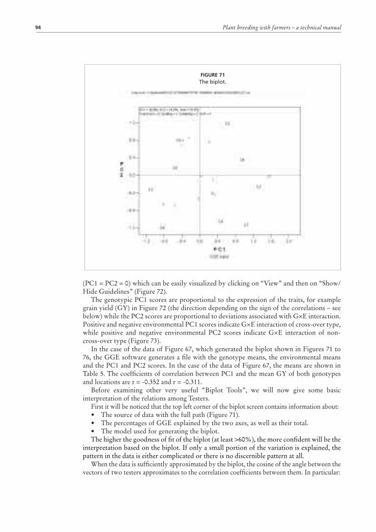
Plant breeding with farmers – a technical manual94
(PC1 = PC2 = 0) which can be easily visualized by clicking on “View” and then on “Show/Hide Guidelines” (Figure 72).
The genotypic PC1 scores are proportional to the expression of the traits, for example grain yield (GY) in Figure 72 (the direction depending on the sign of the correlations – see below) while the PC2 scores are proportional to deviations associated with G×E interaction. Positive and negative environmental PC1 scores indicate G×E interaction of cross-over type, while positive and negative environmental PC2 scores indicate G×E interaction of non-cross-over type (Figure 73).
In the case of the data of Figure 67, which generated the biplot shown in Figures 71 to 76, the GGE software generates a file with the genotype means, the environmental means and the PC1 and PC2 scores. In the case of the data of Figure 67, the means are shown in Table 5. The coefficients of correlation between PC1 and the mean GY of both genotypes and locations are r = -0.352 and r = -0.311.
Before examining other very useful “Biplot Tools”, we will now give some basic interpretation of the relations among Testers.
First it will be noticed that the top left corner of the biplot screen contains information about:• The source of data with the full path (Figure 71).• The percentages of GGE explained by the two axes, as well as their total.• The model used for generating the biplot.The higher the goodness of fit of the biplot (at least >60%), the more confident will be the
interpretation based on the biplot. If only a small portion of the variation is explained, the pattern in the data is either complicated or there is no discernible pattern at all.
When the data is sufficiently approximated by the biplot, the cosine of the angle between the vectors of two testers approximates to the correlation coefficients between them. In particular:
FIGURE 71The biplot.
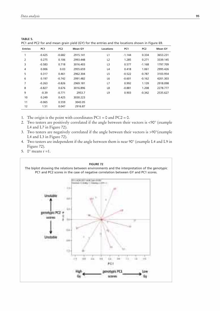
Data analysis 95
TABLE 5. PC1 and PC2 for and mean grain yield (GY) for the entries and the locations shown in Figure 69.
Entries PC1 PC2 Mean GY Locations PC1 PC2 Mean GY
1 -0.425 -0.682 2915.141 L1 -1.144 0.334 3653.231
2 0.275 0.106 2993.448 L2 1.285 0.271 3339.145
3 -0.583 0.718 3016.403 L3 0.577 -1.168 1797.709
4 0.006 0.03 2955.659 L4 0.418 1.061 2995.426
5 0.317 0.461 2962.304 L5 -0.522 -0.787 3103.954
6 0.197 -0.742 2991.482 L6 -0.601 -0.162 4201.303
7 -0.263 -0.826 2969.181 L7 0.992 1.139 2918.098
8 -0.827 0.676 3016.896 L8 -0.881 1.208 2278.777
9 -0.39 -0.771 2953.7 L9 0.903 -0.342 2535.627
10 0.249 0.425 3030.223
11 -0.065 0.559 3043.05
12 1.51 0.047 2916.87
1. The origin is the point with coordinates PC1 = 0 and PC2 = 0.2. Two testers are positively correlated if the angle between their vectors is <90° (example
L4 and L7 in Figure 72).3. Two testers are negatively correlated if the angle between their vectors is >90°(example
L4 and L3 in Figure 72).4. Two testers are independent if the angle between them is near 90° (example L4 and L9 in
Figure 72).5. 0° means r =1.
FIGURE 72The biplot showing the relations between environments and the interpretation of the genotypic
PC1 and PC2 scores in the case of negative correlation between GY and PC1 scores.
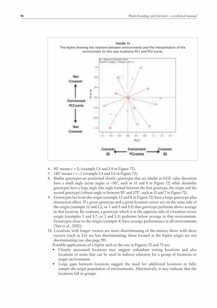
Plant breeding with farmers – a technical manual96
6. 90° means r = 0; (example L5 and L9 in Figure 72).7. 180° means r = -1 (example L4 and L5 in Figure 72).8. Similar genotypes are positioned closely; genotypes that are similar in GGE value directions
have a small angle (acute angles or <90°, such as 10 and 5 in Figure 72) while dissimilar genotypes have a large angle (the angle formed between the first genotype, the origin and the second genotype) (obtuse angle or between 90° and 270°, such as 10 and 7 in Figure 72).
9. Genotypes far from the origin (example 12 and 8 in Figure 72) have a large genotype plus interaction effect. If a given genotype and a given location vector are on the same side of the origin (example 12 and L2, or 1 and 9 and L5) that genotype performs above average in that location. By contrast, a genotype which is at the opposite side of a location vector origin (examples 1 and L7, or 3 and L3) performs below average in that environment. Genotypes close to the origin (example 4) have average performance in all environments (Yan et al., 2000);
10. Locations with longer vectors are more discriminating of the entries; those with short vectors (such as L6) are less discriminating; those located at the biplot origin are not discriminating (see also page 99).
Possible applications of a biplot such as the one in Figures 72 and 73 are:• Closely associated locations may suggest redundant testing locations and also
locations or traits that can be used in indirect selection for a group of locations or target environment.
• Large gaps between locations suggest the need for additional locations to fully sample the target population of environments. Alternatively, it may indicate that the locations fall in groups.
FIGURE 73The biplot showing the relations between environments and the interpretation of the
environment (in this case locations) PC1 and PC2 scores.

Data analysis 97
• The largest angle in a biplot may be used as an indicator of the size of entry by location interaction. The higher the number of negative correlations, the larger the entry × locations interactions.
The accuracy of the relationships among locations as shown in the biplot can be examined by requesting a correlation matrix among testers.
Another very useful function under “Biplot Tools” is the “Which-won-where”.From Biplot Tools, click “Which Won Where/What” and the following will appear on
the biplot (Figure 74):• a polygon that is drawn on entries (in the example, entries 6, 7, 9, 1, 8, 3, 11, 5 and 12)
located away from the biplot origin such that all other entries are contained within the polygon; and
• a set of lines that are radial from the origin and perpendicular through each side of the polygon. These lines form sectors (the area contained between two lines).
In the case of Figure 74, the radial lines divide the biplot into 8 sectors, with each location falling inevitably into one of the sectors. The vertex entry for each sector had the largest values (the winner) among all entries in environments falling within that sector. In this example, entry 12 wins in L9, L2, L4 and L7; entry 8 wins in L1 and L8; entry 6 wins in L3; and entry 9 wins in L5. Therefore the locations are divided into four groups based on the winners.
The average Performance and Stability of the entries can be visualized using “Biplot Tools” and then “Means vs. Stability”. The graph that will appear is shown in Figure 75. The most important features of the graph are:
• a small red circle (in Figure 75 close to genotype 2) indicating the position of the average location, which is defined by the average PC1 and PC2 scores across all locations. This average location can be regarded as a virtual location;
FIGURE 74The “Which-won-where” feature of the biplot.

Plant breeding with farmers – a technical manual98
• a thick red line that passes through the biplot origin and the average location, referred to as the Average-Tester Axis (ATA) or Average Tester Coordination (ATC) Abscissa;
• a red arrow pointing to the average location from the biplot origin; • a thick blue line that passes through the biplot origin and is perpendicular to the ATA;• two blue arrows on the thick blue line, pointing outwards from the biplot origin
(called ATC Ordinate); and• a set of lines parallel to the thick blue line, which starts from the marker of the entries
and project to the ATA. The entries are ranked along the ATA, with the arrow pointing to a greater value according
to their mean performance across all locations. Therefore in this case, the ranking of the entries is Entry 12 (with the highest mean) > Entry 5 > Entry 10 > Entry 11 > Entry 3 > Entry 2 > Entry 8 > Entry 4 > Entry 6 > Entry 1 > Entry 7 > Entry 9.
The blue line separates entries with below-average means from those with above-average means. Thus the rank is: entries 12, 5, 10, 11, 3, 2 and 8 > Grand Mean; entry 4 = Grand Mean; and entries 6, 1, 7 and 9 < Grand Mean.
The vector length of the average location (the distance from biplot origin and the average location marker), relative to the biplot size, is a measure of the relative importance of the entry main effect (G) vs. the entry by location interaction (G×E). The longer it is, the more important is G and the more meaningful the selection based on mean performance. At extremes, a zero average tester vector means G = 0 and therefore the selection based on mean performance is meaningless. In this case the main effect (G) is small as the red circle (the average location) is close to the origin; this could have been anticipated by the spreading of the vectors in Figure 72.
The stability of the entries is graphically represented by the projection from the entry symbol to the blue line. The longer the projection, regardless of the direction, the greater is the entry×location interaction and therefore the lower the stability of the entry across locations. In this case entries 12, 8, 3 and 6 are the least stable, while entries 10 and 5 have the best combination of yield and stability.
FIGURE 75The Mean Performance vs. Stability of entries.

Data analysis 99
When the biplot explains only a small portion of the total variation, some entries may not be as stable as they appear, because they may have greater values in PC3 or PC4. This can be checked by looking at the 3-dimensional biplot: click on biplots and then on 3-D biplot in the drop-down window.
Two features that are very important in the design of MET, including PPB trials are the ability of the environments (locations and/or years) to discriminate the entries and their ability to represent the target environments. These features can be analysed using “Biplot Tools” and then “Discrimination and Representativeness”. The graph that will appear is shown in Figure 76.
The most important features of the graph are:• a small red circle which indicates the average location; • a red line that goes through the biplot origin and the average location (average tester
axis); and• a red arrow pointing to the “ideal” location, which is defined as the ideal location for
testing the entries.The closer a location is located to the “ideal” location, the more desirable it is judged on
both discrimination and representativeness. The ranking of the locations is: L7 > L4 > L2 > L8 > L9 > L1 > L6 > L3 > L5.
The vector length, i.e., the absolute distance between the marker of a location and the plot origin, is a measure of its discriminating ability: the longer the vector, the more discriminating the environment. The absolute length of the projection from the marker of an environment onto the ATC y-axis is a measure of its representativeness: the longer the projection, the less representative the environment. In this case the locations combining better discrimination and representativeness are L7 and L4.
Representativeness is a key factor to decide how a test location should be used in genotype evaluation, assuming adequate discriminating ability (Yan et al., 2007). The representativeness should be measured over a number of years in order to assess its repeatability. A test location
FIGURE 76The discrimination and representativeness of the environments.
Plant breeding with farmers – a technical manual100
must be repeatable across years in ranking genotypes for it to be considered as highly representative and based on repeatability analysis; a highly representative test location, which is also highly repeatable by definition, is ideal for use as core test locations (Yan et al., 2011). In a PPB programme such as the one described in Figure 4, these should be the attributes of the location where to plant the Stage 1 trials, because genotypic differences observed at locations like these are both repeatable across years and representative of the other farmers’ fields in the area. It is crucial for a PPB breeding programme to have test locations of this type.
Genotype × Location and Genotype × Traits interactions in Stage 1 trialsStage 1 trials in either a conventional or participatory breeding programme are normally repeated in a number of locations, commonly as unreplicated or partially replicated trials, as discussed at page 33 and following.
Therefore, the BLUPs generated by the spatial analysis described earlier can be arranged in a series of two-way tables, one for each trait, and analysed with the GGEbiplot software. As an example we will used a Stage 1 trial with 181 genotypes tested in 7 locations. Following the steps shown in Figures 64 to 67, we open the data file that includes the grain yields and farmers score of the 181 genotypes (the rows) in the 7 locations (the columns in Figure 77). Although we will use the grain yield as an example, being one of the most important agronomic traits, the same can be done for any other trait. After following the steps illustrated in Figures 69–71 we obtain the biplot shown in Figure 78.
The biplot explains nearly 50% of the GGE, with most of the locations showing from a strong positive correlation (L5 and L7) to independence (L12 and L7).
FIGURE 77The BLUPs for grain yield (kg/ha) in the left and farmers score (right) obtained from a Stage 1 trial with 181 genotypes (only the first and the last 15 are shown) tested in 7 locations coded
as L3, L5, L7, L10, L11, L12 and L13.

Data analysis 101
Figure 78 can be used to identify the best entries either in specific locations or across locations. This is, however, made considerably easier by using the “Which Won Where/What” feature illustrated earlier, which, in this case, divides the biplot in 8 sectors of which six do not contain any location, one which contains two locations (L11 and L12) with entries such as 58, 68, 26, and 169 as the highest yielding, and one which contains all the other 5 locations and with entries 180 and 181 as winners (Figure 79).
The same process can be repeated using the average farmers’ score (Figure 80). In this case the biplot explains nearly 57% of GGE and the “Which Won Where/What” feature divides the biplot into 10 sectors, 5 of which contain no location (entries that received a low score everywhere), 4 which contain one location each and one which contains 3 locations. This can
FIGURE 78The biplot obtained with the grain yield data of Figure 77.
FIGURE 79The Which Won Where/What biplot obtained with the grain yield data of Figure 77.

Plant breeding with farmers – a technical manual102
be interpreted as an indication that the preferences of the farmers are very specific and that farmers do not select only for grain yield. An interesting case is that of locations L7 and L5, which discriminate similarly among genotypes for grain yield (r = 0.384) but are strongly negatively correlated for farmers’ preferences (r = -0.402) (Table 6).
The most remarkable aspect of Figure 80 is that the classification of the locations is different from the one obtained with grain yield. For example, locations 5 and 7 which were in the same sector for grain yield and strongly and positively correlated, in the case of farmers’ score are strongly and negatively correlated, indicating substantially different preferences by farmers
Should these differences be repeatable over years, they would suggest a danger of classifying locations as similar or dissimilar based on grain yield alone.
Genotype × Location × Year interactions in Stage 2, 3 and 4 trialsUnder "Discussion of results and farmers’ final selection" we introduced files such as those shown in Figures 51 (Stage 2), 55 (Stage 3) and 58 (Stage 4). The common feature of these files is the availability of data from more years (two years for Stage 2, three for Stage 3 and
TABLE 6. Correlation coefficients between grain yield (upper part) and farmers’ scores measures on 181 genotypes grown in six locations.
L3 L5 L7 L10 L11 L12
L5 0.233 1
L7 0.249 0.384 1
L10 0.175 0.200 0.128 1
L11 0.396 0.136 0.100 0.218 1
L12 0.191 0.090 0.078 0.097 0.242 1
L13 0.415 0.188 0.306 0.201 0.278 0.091
L3 L5 L7 L10 L11 L12L5 0.234 1
L7 -0.077 -0.402 1
L10 0.307 -0.068 0.051 1
L11 0.554 0.039 -0.067 0.422 1
L12 0.261 -0.040 -0.056 0.238 0.375 1
L13 0.299 -0.171 0.463 0.294 0.230 0.063
FIGURE 80The Which Won Where/What biplot obtained with the farmers’ score data of Figure 77.

Data analysis 103
four for Stage 4 trials, respectively). It will be noticed that in all these files, in addition to the sheets already discussed, there are some additional sheets that we have not yet discussed. For example, the file shown in Figures 54 and 55 contains additional sheets prepared specifically for the GGEbiplot analysis. Two of these sheets, with the grain yield and the farmers’ score of the year in which the trial was conducted are shown in Figure 81 and the respective biplots in Figure 82. Similar sheets can be organized for all the traits scored in the trial. If needed, different tables can also be combined into one.
The second type of sheets available in the files of the Stage 2, 3 and 4 trials are those compiled using all the data available, i.e. two years of data in Stage 2, three years of data in Stage 3 and four years of data in Stage 4. For example, using the Stage 3 trial already shown in Figure 55, we can collect from the sheet “Table 2 (3Y)” all the grain yield data (gy07 from Stage 1, gy08_F1, gy08_F2 and gy08_F3 from Stage 2, and gy09_F1, gy09_F2 and gy09_F3 from Stage 3) and with “copy” and “paste” we can organize them as shown in a new sheet named, for example “GGEGY3Y” shown on the left side of Figure 83. The same can be done for all the other traits for which data are available in “Table 2 (3Y)” of Figure 55 as for example for the farmers’ scores shown on the right side of Figure 83.
It will be noticed that there are a number of missing data in the sheets shown in Figure 83 as entries nos. 6 and 12 were added as checks only in the Stage 3 trial. The addition of checks in the course of a PPB programme is very frequent as a consequence of the continuous adoption of new varieties. This was the case for the entries 6 and 12 that farmers adopted from previous breeding cycles and asked to introduce as additional checks in the PPB trial.
FIGURE 81The grain yield (left) and the farmer score (right) in a Stage 3 trial conducted in three farmers’ fields.

Plant breeding with farmers – a technical manual104
This example will allow us to explore two additional features of the GGEbiplot software. By following the steps illustrated earlier we obtain the biplot shown in Figure 84, in
which the 7 environments, which in this case represent 3 years and 3 different farmers’ fields in the same village, are divided into three groups: one with 4 environments and entry 4 as the
FIGURE 82The biplots of the grain yield (left) and the farmer score (right) in a Stage 3 trial shown in Figure 80.
FIGURE 83 Three years data on grain yield (left) and farmers’ score (right) from Figure 68 and arranged for biplot analysis.
Data analysis 105
winner; one with two environments and entry 6 (one of those with missing data) as winner; and one with only one environment and with entry 3 as the only entry yielding slightly more than average. One sector includes entry 12 (the second entry with missing data) and no environments.
FIGURE 84The Biplot for grain yield of 12 varieties in 7 environments using the data of Figure 83 (left).
FIGURE 85The biplot of Figure 84 after editing.

Plant breeding with farmers – a technical manual106
FIGURE 86The option to run the biplot analysis with a subset of either entries or testers.
FIGURE 87The choice of the entries to keep and those to remove.

Data analysis 107
The first new feature of the GGEbiplot software is “Format” which allows us to name the biplot, edit the colour and fonts of the lines, testers and entries, and change the plot size. In this way it is possible to edit the biplot and make it ready for a publication. An example of how a biplot may look like after editing is shown as in Figure 82.
The second feature of the GGEbiplot software is the possibility it offers to run subsets of the original data set by deleting either entries or testers: this is useful, for example, in the case where the biplot explain only a small part of GGE because of one tester, or in cases like the one in Figure 83, to test the effect of the entries with missing data on the relationships between entries and between testers.
This is done by clicking “Data” on the menu bar followed by “Run ANY subset by....” (Figure 86). This will bring to the window shown in Figure 87 that allows choosing the entries to keep and those to delete. After the choice is made, by pressing “Confirm” a new biplot is generated without entries 6 and 12 (Figure 88).
By comparing the two biplots (Figures 84 and 88) it will be noticed that most of the locations are now included in the same sector (GY08_F2 and GY09_F1 are nearly at the margin of this sector) in which the winner is still entry 4, and entry 1, which was in a sector with no locations, is now in the same sector as location GY08_F1.
Relationships between traitsThe biplot can also be exploited to analyse the relationships between traits. The data file to be used, one for each location, is shown in Figure 89.
To display the genotype × trait two-way data in a biplot, the following formula is used: (Tij - Tj)/sj = λ1ζi1τj1 + λ2ζi2τj2 + εij
where Tij is the average value of genotype i for trait j, Tj is the average value of trait j over all genotypes,
FIGURE 88The biplot of Figure 84 without entries 6 and 12.
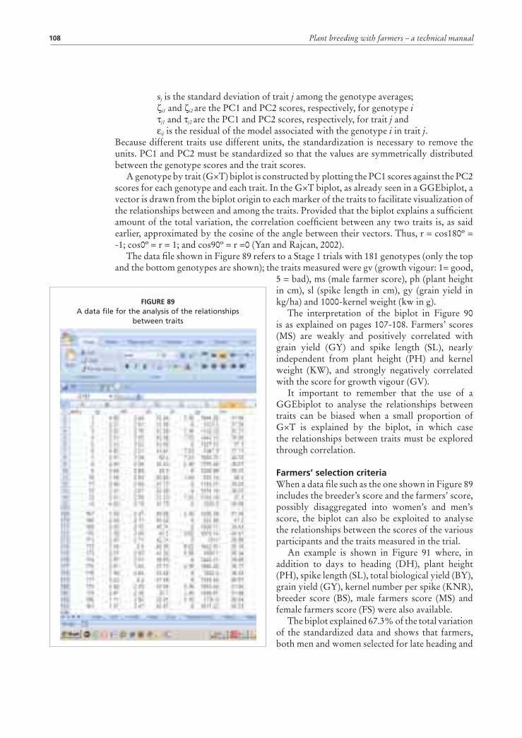
Plant breeding with farmers – a technical manual108
sj is the standard deviation of trait j among the genotype averages; ζi1 and ζi2 are the PC1 and PC2 scores, respectively, for genotype i τj1 and τj2 are the PC1 and PC2 scores, respectively, for trait j and εij is the residual of the model associated with the genotype i in trait j. Because different traits use different units, the standardization is necessary to remove the units. PC1 and PC2 must be standardized so that the values are symmetrically distributed between the genotype scores and the trait scores.
A genotype by trait (G×T) biplot is constructed by plotting the PC1 scores against the PC2 scores for each genotype and each trait. In the G×T biplot, as already seen in a GGEbiplot, a vector is drawn from the biplot origin to each marker of the traits to facilitate visualization of the relationships between and among the traits. Provided that the biplot explains a sufficient amount of the total variation, the correlation coefficient between any two traits is, as said earlier, approximated by the cosine of the angle between their vectors. Thus, r = cos180º = -1; cos0º = r = 1; and cos90º = r =0 (Yan and Rajcan, 2002).
The data file shown in Figure 89 refers to a Stage 1 trials with 181 genotypes (only the top and the bottom genotypes are shown); the traits measured were gv (growth vigour: 1= good,
5 = bad), ms (male farmer score), ph (plant height in cm), sl (spike length in cm), gy (grain yield in kg/ha) and 1000-kernel weight (kw in g).
The interpretation of the biplot in Figure 90 is as explained on pages 107-108. Farmers’ scores (MS) are weakly and positively correlated with grain yield (GY) and spike length (SL), nearly independent from plant height (PH) and kernel weight (KW), and strongly negatively correlated with the score for growth vigour (GV).
It important to remember that the use of a GGEbiplot to analyse the relationships between traits can be biased when a small proportion of G×T is explained by the biplot, in which case the relationships between traits must be explored through correlation.
Farmers’ selection criteriaWhen a data file such as the one shown in Figure 89 includes the breeder’s score and the farmers’ score, possibly disaggregated into women’s and men’s score, the biplot can also be exploited to analyse the relationships between the scores of the various participants and the traits measured in the trial.
An example is shown in Figure 91 where, in addition to days to heading (DH), plant height (PH), spike length (SL), total biological yield (BY), grain yield (GY), kernel number per spike (KNR), breeder score (BS), male farmers score (MS) and female farmers score (FS) were also available.
The biplot explained 67.3% of the total variation of the standardized data and shows that farmers, both men and women selected for late heading and
FIGURE 89A data file for the analysis of the relationships
between traits

Data analysis 109
FIGURE 90A G×T biplot of the data shown in Figure 87.
FIGURE 91A biplot showing the relationships between farmers’ (men and women) and breeder’s score
and a number of traits in a trial with 21 entries.

Plant breeding with farmers – a technical manual110
tall lines (the vectors for DH, MS, FS and PH are all in the same direction and with relatively narrow angles between them). There was an almost complete agreement between men and women scores, at least for the traits measured in this experiment.
In contrast, the breeder score was closely associated with grain yield and biological yield, and also associated with spike length and kernel number, but not as closely. As the angle between the BS vector and both the MS and the FS vectors is nearly 90°, farmers selection and breeder selection are nearly independent.
Another example of how the use of the biplots can clarify the selection criteria of the farmers is given in Figure 92. The biplot on the left-hand side (A) shows a nearly zero correlation between farmers’ score (ignoring farmers’ field no. 1, which is too short to be meaningful) and grain yields. On the right-hand side (B), this lack of correlation is explained by a strong preference by farmers for tall genotypes, as shown by the narrow angles between the vectors for farmers’ scores (FS) and plant height (PH) in each of the four farmers’ fields.
FIGURE 92A biplot (A) showing the relationships between farmers’ score (FS) and grain yield (GY) in a Stage 3 trial planted
in four farmers’ fields. B is the same biplot with the addition of plant height (PH).

111
Variety release and seed production
The potential advantages of PPB, such as faster dissemination of new varieties, higher adoption, and increased biodiversity within the crop, will not be realized unless the seed of the new varieties is available in sufficient amounts to all the farmer community. In many countries, seed is produced only after a variety is officially released. Variety release is decided by a government-appointed committee (the variety release committee) based on a scientific report on the performance, agronomic characteristics, reaction to pests and disease and quality characteristics of the new variety. Farmers’ opinions are not sought. As a result, there are several cases of near-zero adoption of released varieties, and widespread adoption of varieties that have not been released. In these cases, the considerable investment made in developing the new variety and in producing its seed has been wasted.
A number of problems have been identified in the system of variety testing in relation to variety release (Tripp et al., 1997). Of these, the most relevant to the adoption (or lack of it) are:1. Inappropriate site selection In some cases the sites are actually within research stations
and not in farmers’ fields. 2. Unrepresentative trial management Usually the level of inputs, particularly of
fertilizers, are higher than those used by the majority of the farmers; the same applies to the crop rotation, which, in the best of the cases is only one of those used by the farmers.
3. Trial analysis is biased against poor environments Usually sites with low or variable yields and with some entries failing to give a measurable yield are discarded from the analysis (Finlay and Wilkinson, 1963).
4. Use of sub-optimal experimental designs and statistical analysis For example, little or no use of spatial analysis and use of unweighted means across sites which because of scale effect leads to the selection of the highest yielding entries in the highest yielding sites.
5. Lack of farmer participation Farmers are only involved in providing the land for the trials, and no attention is given to farmer-preferred variety traits.
An example of how inefficient and ineffective such a variety testing and release system can be is given by Syria, where three varieties rejected by the variety release committee were later widely adopted by farmers after the three varieties were included in the PPB programme (ICARDA, 2006).
PPB addresses this issue directly, by turning the delivery phase of a plant breeding programme upside down (Figure 93). In conventional breeding, the most promising lines are released, their seed is produced under controlled conditions (certified seed) and only then do farmers decide whether or not to adopt the new variety. Therefore, the entire process is supply-driven. As a consequence, and also because of the problems associated with variety testing described earlier, in many developing countries many varieties are produced and released but only a small fraction of these are adopted. In a PPB programme, the decision on which variety to release depends on initial adoption by farmers during the four stages of selection, and the process is therefore demand-driven. This is expected to increase adoption rates, and also to reduce production risks, since farmers gain knowledge of the variety’s performance under various agronomic practices, soil types and rainfall amounts as part of the selection process. Last, but not least, the institutional investment in seed production is nearly always repaid by farmers’ adoption.

Plant breeding with farmers – a technical manual112
Implementation of PPB requires changes both in variety release procedures and in the seed sector. Interestingly these changes are included in Article 6 (g) of the International Treaty on Plant Genetic Resources for Food and Agriculture (www.fao.org/nr/cgrfa):
“The sustainable use of plant genetic resources for food and agriculture may include such measures as:
reviewing, and, as appropriate, adjusting breeding strategies and regulations concerning variety release and
seed distribution.”
Also, a recent report to the United Nations (De Schutter, 2009) refers to this issue in recommending the Member States to:
“a. Ensure that their seed regulations (seed certification schemes) and their programmes to support access
to seeds do not lead to an exclusion of farmers’ varieties. Instead, the development of such varieties should
be encouraged by including efficient traditional seed varieties in government approved seed lists as well
as subsidized seed distribution programmes, as well as by participatory plant breeding and farmer field
schools;
b. Support and scale up local seed exchange systems such as community seed banks and seed fairs, and
community registers of peasant varieties, and use them as a tool to improve the situation of the most
vulnerable groups, i.e. through the granting to the poorest seedless farmers of seed vouchers which can be
exchanged for seed at the fair. States should develop incentives for the wider use of food products made out
of farmers’ varieties in processing and marketing, or through public procurements schemes, as in school-
feeding programmes;”
Conventional plant breeding and the formal seed sector have been successful in providing seeds of improved varieties of some important staple or cash crops to farmers in favourable areas. However, the policy, regulatory, technical and institutional environment under which these institutions operate limits their ability to serve the diverse needs of small-scale farmers in marginal environments and remote parts of developing countries.
FIGURE 93Conventional plant breeding is typically supply-driven; new varieties are released before
knowing whether or not farmers like them. Participatory plant breeding is demand-driven; the delivery phase is driven by the initial adoption by farmers at the end of a full cycle of selection.

Variety release and seed production 113
We must remember that most of today’s farmers’ work supplies about 70 percent of all the world’s food – 90 percent in countries like Nigeria. Industrial farming that is now called “conventional” accounts for only 30 percent of the total world output and has existed for only about a century, which is less than one percent of the total known history of agriculture (Pimbert, 2011).
The model of seed production we are implementing (Figure 94) integrates the formal and the informal seed systems. Seed requirements for PPB trials are 50 –100 kg per variety in the case of winter cereals, with 15 to 30 varieties being tested in each village. This seed is produced in the village and cleaned and treated using locally manufactured small seed cleaners that can process about 400 kg of seed per hour. For the large-scale trials, requirements are a few tonnes per variety per farmer, and 2 or 3 varieties are tested in each village. At this stage, seed production is still handled at village level, using locally manufactured larger equipment capable of cleaning and treating 1 tonne of seed per hour. Production is now supervised by staff of the Seed Organization (a Governmental Body). The procedure for variety release can be initiated at this stage. If initial adoption if followed by wider demand for seed, the variety is released, and the formal seed system can initiate large-scale seed production using as a starting point the few tonnes of seeds produced in the villages.
In most developing countries, the majority of the seed used is produced by the informal seed system. In this situation, the PPB model shown in Figure 94 can provide the informal system with quality seed of improved varieties through path 2.
FIGURE 94Linking participatory plant breeding and variety release with the formal (path 1)
and informal (path 2) seed production approaches.


115
The impact of plant breeding
This section is based on two recent reviews of impact assessment of plant breeding (Morris and Heisey, 2003) and of PPB (Ashby 2009).
CONVENTIONAL PLANT BREEDINGPlant breeding research generates benefits only when the improved varieties are adopted by farmers. However, contrary to private breeding programmes, most public breeding programmes still value variety release, whether or not it is followed by actual adoption. Similarly, the credentials of public breeders are commonly based on variety release.
Because farmers decide, ultimately, which varieties are sown, numerous studies have been conducted on the determinants of adoption of improved varieties in less developed countries (LDCs). Despite considerable diversity between sites (Heisey and Mwangi, 1993), empirical evidence points to a number of common factors that influence the adoption of improved varieties in a wide range of farming systems. These factors include the level of education of the farmer, their resource base, the availability of credit and the intensity of demonstrations and extension work (Dixon et al., 2006). Risk may also tend to act as an impediment to adoption of improved practices and Anderson (1974) has used stochastic dominance to identify less risky new practices that would be preferred by “risk-adverse” farmers.
Once the varieties are adopted, the benefits vary: higher yields, improved quality, lower production costs, simplified crop management requirements or shorter cropping cycles (Morris and Heisey, 2003). The size and the value of the benefits depend on the area planted to the improved varieties. Therefore, the first step in calculating the benefits of plant breeding research is to estimate the area planted to improved varieties. In principle, this should be easy. In practice, it is often difficult. The difficulty is associated with the definition “improved variety”, which may not be readily identifiable (for example, if the improvement is for a quality only measurable through a laboratory test), and may not remain always the same (for example if farmers use their own seed for a number of years and if they practise some forms of selection). The second step is to decide whether to measure adoption at a given point in time, or to follow adoption over time.
To assess area planted to improved varieties, three types of data are commonly used, namely: (1) farm-level survey data, (2) seed sales data, and (3) expert opinion. Each of the three types of data has advantages and disadvantages.
The use of farm-level survey data is the most reliable way to estimate the area planted to improved varieties, but such data are rarely available, because surveys are expensive and time consuming to conduct. Even when they are available, the spatial and/or temporal coverage is often incomplete.
Use of seed sales data has four potential problems, namely (1) they usually do not include data on farm-saved seed or seed produced outside the formal seed sector; (2) even when most seed planted is commercial seed, data on commercial seed sales must be treated with caution, because seed organizations may have incentives to misrepresent their production and sales figures; (3) this method gives incorrect results if there are significant discrepancies between the amount of seed produced, the amount of seed sold, the amount of seed planted, and the proportion of the planted area that is harvested; and (4) reliable information about farmers’ actual planting rates may not be available.
Plant breeding with farmers – a technical manual116
The use of expert opinion refers to individuals who can ‘guesstimate’ with a reasonable degree of accuracy the area planted with improved varieties. The estimates based on expert opinion can be quite accurate, but the danger is that certain individuals may have incentives to provide biased estimates. Therefore, it is advisable to survey several experts and to base the estimate on the consensus.
For some types of impact studies, it is desirable to estimate not only the area planted to improved varieties at a specific point in time, but also the rate of diffusion of improved varieties over time. The diffusion rate of an improved variety can be expressed in terms of the percentage of the area planted to the improved variety, or in terms of the percentage of farmers using the improved variety. Most studies on improved varieties diffusion assume that the cumulative proportion of the area planted to improved varieties follows the S-shaped or ‘logistic’ pattern (Rogers, 1962) which is based on the assumptions that (1) the population of potential adopters is large and non-homogeneous, with unequal access to information about innovations and differing in their willingness to innovate, and (2) technology adoption is non-reversible. When the first assumption is violated, the probability increases that the diffusion path will diverge from the expected smooth S-shaped function and therefore the method is more appropriate for estimating the diffusion of improved varieties over an extended period and across a large area. Also, the second assumption is not always met. Farmers often take up a new technology, experiment with it for some time, and then discontinue using it. In the case of improved varieties, disadoption can occur for a number of reasons, and there are plenty of examples in which improved varieties have been introduced into areas where they were not well adapted, with disappointing results. Alternatively, changes in external factors may over time erode the profitability of improved varieties, such as when rising fertilizer prices reduce the returns to investing in hybrid seed. Finally, a good improved variety may be replaced by a better variety. Given the possibility of disadoption, use of the classic upward-sloping logistic curve may be inappropriate (Morris and Heisey, 2003).
PARTICIPATORY PLANT BREEDINGThe impact of a PPB programme is generally more complex to analyse than conventional plant breeding because the impact of PPB is multifaceted and includes changes in the research process as well as in knowledge, technology design and social organization (Ashby, 2009).
Typical impacts of a PPB programmes are (Ashby, 2009; http://impact.cgiar.org/assessing-economic-impact-participatory-and-conventional-barley-breeding-programs-jordan; http://impact.cgiar.org/assessing-benefits-and-costs-participatory-and-conventional-barley-breeding-programs-syria):
• varieties emerge that are well tailored to poor producers’ needs; • a shorter time is needed to get appropriate materials into farmers’ fields and therefore
accelerate adoption and seed dissemination, thus improving research efficiency;• maintenance of or increased agro-biodiversity in farmers’ fields; • improvement in farmers’ organizational and social capital, as well as individual
farmers’ knowledge and skills and capacity to learn and experiment;• increased poor farmers’ access to improved varieties, their productivity, nutrition,
marketing and incomes, and thus a more resilient and sustainable farming system; and• improved gender equity.Some PPB impacts, such as the variety adoption can be analysed using some of the
methods described above for conventional plant breeding. The type of data more suitable to PPB would be the farm-level survey data and the expert opinion. Seed sales data may not be available, as in several countries the seed of PPB varieties cannot be legally commercialized if the varieties are not officially released. Given the rigidity of the variety release system, it
The impact of plant breeding 117
is usually difficult to obtain official release of PPB varieties, even though some exceptions are known.
Another impact that in theory is not difficult to measure is the impact on biodiversity. This could also be based on farm-level survey data and expert opinion to collect information on an annual basis on the number of different varieties that farmers select from the PPB programmes and decide to grow as their crop. In such a case, the actual area planted with each variety is irrelevant, because due to the cyclic nature of the programme, there is rapid variety replacement and therefore it is usually the exception rather than the rule that a single PPB variety covers a large area. A one-time survey will only measure the spatial dimension of the biodiversity increase, and therefore the data from the farm-level survey data and the expert opinion should be collected on a continuous basis to measure the temporal dimension of biodiversity change. For example, in the PPB programme on barley in Syria (Ceccarelli and Grando, 2009; Ceccarelli et al., 2012) and during the last five cropping seasons (2005/6 to 2010/11), the farmers have adopted, in areas from a few hundred to several thousand hectares, 93 new varieties (ranging from pure lines to populations). This compares with a total of 7 varieties released by conventional plant breeding during the last 35 years.
The impact of PPB has been documented by Ashby (2009) with examples for cassava in Brazil and Colombia; pearl millet in Namibia and in India; maize in Mali, India, Ethiopia, Honduras and Brazil; beans in Colombia, United Republic of Tanzania, Ethiopia and Rwanda; potatoes in Rwanda, Bolivia, Peru, Ecuador and the Netherlands (Lammerts van Bueren et al., 2009); rainfed rice in India; rice in Bangladesh, India, Nepal and in East India; and barley in the Syrian Arab Republic, Jordan, Eritrea, Morocco, Tunisia, Iran, Egypt and Yemen.
However, other impacts mentioned above that are external to the technology, and that are often referred to as disembodied effects, pose a greater challenge for impact assessment as they are more difficult to quantify (Lilja and Dixon, 2008).

119
Conclusions
The main conclusion is that it is entirely possible to organize a plant breeding programme with the full participation of farmers while maintaining intact the “science” of plant breeding. Therefore, from a scientific point of view there should be no scientific objections to using PPB.
Biodiversity, climate change and hunger are among the most frequently debated global problems. The three problems are related to each other, and PPB can make a contribution to all three of them.
The continuous decrease of biodiversity has been widely documented (World Conservation Monitoring Centre, 1992; Butchart et al., 2010; Frison, Cherfas and Hodgkin, 2011) as well as the effects of climate changes. In addition we have seen at the beginning of this manual that hunger as well as hidden hunger is still widespread.
Recently, a recent report to the United Nations (De Schutter, 2009) establishes a relationship between agrobiodiversity, seed systems, hunger and participatory plant breeding. It underlines that hunger is not only a problem of production, but also a problem of accessibility and availability, and it recommends (Para. 57 (b)) that donors and international institutions, including the Consultative Group on International Agricultural Research and FAO, should, in particular:
• Support efforts by developing countries to establish a regime for the protection of intellectual property rights which suits their development needs and is based on human rights: (i) by refraining from imposing on these countries the condition that they go beyond the minimum requirements of the TRIPS Agreement, particularly by the insertion of “TRIPS-plus” provisions in free trade agreements; (ii) by encouraging the provision of technical advice to developing countries that facilitates the adoption of sui generis systems for the protection of plant varieties, including by UPOV and WIPO, consistent with the status of WIPO as specialized agency of the United Nations system and with its Development Agenda, which imposes a duty on WIPO to mainstream human rights into its activities and to enhance the development dimension of its activities; and (iii) by prohibiting the use of contractual clauses (technology use agreements) or genetic use restriction technologies (GURTs) in genetically modified seeds by seed suppliers, whenever they rely on such clauses or technology in order to strengthen the protection of their privileges beyond the balance adopted by the legislator between the interest of suppliers and broader social goals;
• Fund breeding projects on a large diversity of crops, including orphan crops, as well as on varieties for complex agro-environments such as dry regions, and not only in breadbasket regions, in order to address the needs of the most vulnerable groups;
• Put farmers at the centre of research through participatory research schemes such as participatory plant breeding; and
• Channel an adequate proportion of funds towards research programmes and projects that aim at improving the whole agricultural system and not only the plant (agroforestry, better soil management techniques, composting, water management, good agronomic practices), as well as towards institutional innovations (such as community seed banks, seed fairs and farmer field schools).

Plant breeding with farmers – a technical manual120
Therefore, PPB is now recommended by two international documents as one way of addressing the needs of all those farmers who have been bypassed by conventional plant breeding.
Ultimately, participatory plant breeding is able to combine the maintenance and the enhancement of agrobiodiversity with the need to feed everybody by making the food available and accessible, and with the need to cope with a continuous and gradual change in the climatic conditions.

121
References
Almekinders, C. & Hardon, J. (editors). 2006. Bringing farmers back into breeding. Experiences
with participatory plant breeding and challenges for institutionalisation. Agromisa Special No. 5. Agromisa, Wageningen, The Netherlands. 140 p.
Anderson, J.R. 1974. Risk efficiency in the interpretation of agricultural production research. Review of Marketing and Agricultural Economics, 42: 131–184.
Annicchiarico, P., Bellah, F. & Chiari, T. 2005. Defining subregions and estimating benefits for a specific-adaptation strategy by breeding programs: a case study. Crop Science, 45: 1741–1749.
Annicchiarico, P., Bellah, F. & Chiari, T. 2006. Repeatable genotype × location interaction and its exploitation by conventional and GIS-based cultivar recommendation for durum wheat in Algeria. European Journal of Agronomy, 24: 70–81.
Ashby, J.A. & Lilja, N. 2004. Participatory research: Does it work? Evidence from Participatory Plant Breeding. In: New Directions for a Diverse Planet. Proceeding of the 4th International Crop Science Congress, Brisbane, Queensland, Australia, 26 September–1 October 2004.
Ashby, J.A. 2009. The impact of participatory plant breeding. pp. 649–671, in: S. Ceccarelli, E.P. Guimaraes and E. Weltzien (editors). Plant Breeding and Farmer Participation. FAO, Rome, Italy.
Bänziger, M. & Cooper, M. 2001. Breeding for low input conditions and consequences for participatory plant breeding: Examples from tropical maize and wheat. Euphytica, 122: 503–519
Bellon, M.R. [2006; online]. Crop research to benefit poor farmers in marginal areas of the developing world: a review of technical challenges and tools. CAB Reviews: Perspectives in
Agriculture, Veterinary Science, Nutrition and Natural Resources.
Bishaw, Z. & van Gastel, A.J.G. 2009. Variety release and policy options. pp. 565–587, in: S. Ceccarelli, E.P. Guimaraes and E. Weltzien (editors). Plant Breeding and Farmer Participation. FAO, Rome, Italy.
Butchart, S.H.M., Walpole, M., Collen, B. and 42 others. 2010. Global Biodiversity: Indicators of Recent Declines. Science, 328(5982): 1164–1168.
Byerlee, D 1994. Modern varieties, productivity, and sustainability: Recent experiences and emerging challenges. CIMMYT, Mexico.
Biggs, S.D. & Farrington, J. 1991. Agricultural research and the rural poor: a review of social science analysis. International Development Research Centre (IDRC), Ottawa, Canada. 139 p.
Ceccarelli, S. 1989. Wide adaptation. How wide? Euphytica, 40: 197–205.Ceccarelli, S. 2009a. Main stages of a plant breeding programme pp. 63–74, , in: S. Ceccarelli, E.P.
Guimaraes and E. Weltzien (editors). Plant Breeding and Farmer Participation. FAO, Rome, Italy.
Ceccarelli, S. 2009b. Selection methods. Part 1: Organizational aspects of a plant breeding programme pp. 63–74, in: S. Ceccarelli, E.P. Guimaraes and E. Weltzien (editors). Plant
Breeding and Farmer Participation. FAO, Rome, Italy.Ceccarelli, S. 2011. People I have known. PRGA Programme Working Document no. 28. PRGA
Program, Cali, Colombia.Ceccarelli, S. & Grando, S. 2009. Participatory plant breeding in cereals. In: M.J. Carena
(editor). Cereals. Handbook on Plant Breeding, Vol. 3. Springer, New York, USA.Ceccarelli, S., Galié, A., Mustafa, Y. & Grando, S. 2012. Syria: Participatory barley breeding—
farmers’ input becomes everyone’s gain. pp. 53-66, in: M. Ruiz & R. Vernooy (editors). The

Plant breeding with farmers – a technical manual122
Custodians of biodiversity: sharing access and benefits to genetic resources. Earthscan, 2 Park Square, Milton Park, Abingdon, Oxon OX14 4RN.
Ceccarelli, S., Guimaraes, E.P. & Weltzien, E. (editors). 2009 Plant Breeding and Farmer
Participation. FAO, Rome, Italy. 671 p.Ceccarelli, S., Grando, S., Tutwiler, R., Baha, J., Martini, A.M., Salahieh, H., Goodchild, A.
& Michael, M. 2000. A methodological study on participatory barley breeding. I. Selection phase. Euphytica, 111: 91–104.
Ceccarelli, S., Grando, S., Amri, A., Asaad, F.A., Benbelkacem, A., Harrabi, M., Maatougui, M., Mekni, M.S., Mimoun, H., El–Einen, R.A., El–Felah, M., El–Sayed, A.F., Shreidi, A.S. & Yahyaoui, A. 2001. Decentralized and participatory plant breeding for marginal environments. pp. 115–136, in: H.D. Cooper, C. Spillane and T. Hodgin (editors). Broadening the Genetic
Base of Crop Production. CABI, New York, USA/FAO, Rome, Italy/IPGRI, Rome, Italy.Ceccarelli, S., Grando, S., Singh, M., Michael, M., Shikho, A., Al Issa, M., Al Saleh, A.,
Kaleonjy, G., Al Ghanem, S.M., Al Hasan, A.L., Dalla, H., Basha, S. & Basha, T. 2003. A methodological study on participatory barley breeding. II. Response to selection. Euphytica, 133: 185–200.
Cooper, M., Stucker, R.E., DeLacy, I.H. & Harch, B.D. 1997. Wheat breeding nurseries, target environments, and indirect selection for grain yield. Crop Science, 37: 1168–1176.
Cullis, B.R., Smith, A.B. & Coombes, N.E. 2006. On the design of early generation variety trials with correlated data. Journal of Agricultural, Biological and Environmental Statistics, 11: 381–393.
Coombes, N.E. 2006. DiGGer, a Design Generator. See: http://www.austatgen.org/files/software/downloads.
De Schutter, O. 2009. Seed policies and the right to food: enhancing agrobiodiversity and encouraging innovation. Report presented to the UN General Assembly (64th session) (UN doc. A/64/170). Available at http://www.srfood.org/images/stories/pdf/officialreports/20091021_report-ga64_seed-policies-and-the-right-to-food_en.pdf Accessed 01 March 2012
Dixon, J., Nalley, L., Kosina, P., La Rovere, R., Hellin, J., Aquino, P. 2006. Adoption and economic impact of improved wheat varieties in the developing world. Journal of Agricultural
Science, 144: 489–502.Duvick, D.N. 2009. Selection methods. Part 3: Hybrid breeding. pp. 229–258, in: S. Ceccarelli,
E.P. Guimaraes and E. Weltzien (editors). Plant Breeding and Farmer Participation. FAO, Rome, Italy.
Dvorak, K.A. 1987. A social science perspective on evaluating and designing component research: A case study of nitrogen fertilizer and post-rainy season sorghum in India. Workshop on Social Science Perspectives in Managing Agricultural Technololgy, 24–27 September 1986, Lahore, Pakistan.
Eisemann, R.L., Cooper, M. & Woodruff, D.R. 1990. Beyond the analytical methodology: better interpretation and exploitation of genotype-by-environment interaction in breeding. pp. 108–117, in: M.S. Kang (editor). Genotype-by-Environment Interaction and Plant
Breeding. Department of Agronomy, Louisiana State Agricultural Experiment Station, Baton Rouge, USA.
Fehr, W.R. (editor). 1984. Genetic contributions to yield gains of five major crop plants. CSSA Special Publication No. 7. ASA and CSSA, Madison, WI, USA.
Finlay, K.W. & Wilkinson, G.H. 1963. The analysis of adaptation in a plant breeding programme. Australian Journal Agricultural Research, 14: 742–754.
Foresight. 2011. The Future of Food and Farming, 2011. Executive Summary. The Government Office for Science, London, UK.
Frison, E.A., Cherfas, J. & Hodgkin, T. 2011. Agricultural biodiversity is essential for a sustainable improvement in food and nutrition security. Sustainability, 3: 238–253.
References 123
Gabriel, K.R. 1971. The bi-plot graphic display of matrices with application to principal component analysis. Biometrika, 58: 453–467.
Gauch, H.G. & Zobel, R.W. 1996. AMMI analysis of yield trials. pp. 1–40, in: M.S. Kang and H.G. Gauch (editors). Genotype-by-environment interaction. CRC Press, Boca Raton, FL, USA.
Gepts, P. & Hancock, J. 2006. The future of plant breeding. Crop Science, 46: 1630–1634.Gibson, R.W., Byamukama, E., Mpembe, I., Kayongo, J. & Mwanga, R.O.M. 2008. Working
with farmer groups in Uganda to develop new sweet potato cultivars: decentralisation and building on traditional approaches. Euphytica, 159: 217–228.
Grüneberg, W., Mwanga, R., Andrade, M. & Espinoza, J. 2009. Selection methods. Part 5: Breeding clonally propagated crops. pp 275-322, in: S. Ceccarelli, E.P. Guimaraes and E. Weltzien (editors). Plant Breeding and Farmer Participation. FAO, Rome, Italy.
Heisey, P. & Mwangi, W. 1993. An overview of measuring research impacts assessment. pp. 28–36, in: P. Heisey and S. Waddington (editors). Impacts on Farm Research. Proceedings of a Networkshop on Impacts on Farm Research in Eastern Africa. CIMMYT Eastern and Southern Africa On-Farm Research Network Report, No. 24. CIMMYT, Harare, Zimbabwe.
ICARDA [International Center for Agricultural Research in the Dry Areas]. 2006. Annual Report. ICARDA, Aleppo, Syria.
IAASTD. 2009. Agriculture at a crossroads. International Assessment of Agricultural Knowledge, Science, and Technology for Development Global Report. The Island Press, Washington D.C., USA.
Joshi, K.D., Sthapit, B.R. & Witcombe, J.R. 2001. How narrowly adapted are the products of decentralized breeding? The spread of rice varieties from a participatory plant breeding programme in Nepal. Euphytica, 122: 589–597.
Kempton, R.A. & Gleeson, A. 1997. Unreplicated trials. pp. 86–100, in: R.A. Kempton and P.N. Fox (editors). Statistical Methods for Plant Variety Evaluation. Chapman & Hall, London, UK.
Lammerts van Bueren, E.T., Hutten, R., Tiemens-Hulscher, M. & Vos, N. 2009. Developing collaborative strategies for breeding for organic potatoes in the Netherlands. pp. 176–181, in:
Z. Hoeschkel (editor). Breeding Diversity. Proceedings of the First International IFOAM Conference on Organic Animal and Plant Breeding, 25–28 August 2009, Santa Fe, New Mexico, USA.
Lammerts van Bueren, E.T. & Myers, J.R. (editors). In press. Organic Crop Breeding. Wiley-Blackwell Publishing, Hoboken, NJ, USA.
Lantican, M.A., Dubin, H.J. & Morris, M.L. 2005. Impacts of international wheat breeding research in the developing world, 1988–2002. CIMMYT, Mexico.
Lilja, N. & Ashby, J.A. 1999a. Types of participatory research based on locus of decision-making. Consultative Group on International Agricultural Research (CGIAR), Participatory Research and Gender Analysis (PRGA). PRGA Working Document No. 6.
Lilja, N. & Ashby, J.A. 1999b. Types of gender analysis in natural resource management and plant breeding. Consultative Group on International Agricultural Research (CGIAR), Participatory Research and Gender Analysis (PRGA). PRGA Working Document No. 8.
Lilja, N. & Dixon, J. 2008. Responding to the challenges of impact assessment of participatory research and gender analysis. Paper prepared for the Workshop on Rethinking Impact:
Capturing the Complexity of poverty and Change. PRGA Program, CIAT, Cali, Colombia. March, 2008.
Machado, A.T. & Fernandes, M.S. 2001. Participatory maize breeding for low nitrogen tolerance. Euphytica, 122: 567–573.
Manu-Aduening, J.A., Lamboll, R.I., Ampong Mensah, G., Lamptey, J.N., Moses, E., Dankyi, A.A. & Gibson, R.W. 2006. Development of superior cassava cultivars in Ghana by

Plant breeding with farmers – a technical manual124
farmers and scientists: The process adopted, outcomes and contributions, and changed roles of different stakeholders. Euphytica, 150: 47–61.
Mekbib, F. 1997. Farmer participation in common bean genotype evaluation: The case of eastern Ethiopia. Experimental Agriculture, 33: 399–408.
McGuire, S., Manicad, G. & Sperling, L. 1999. Technical and institutional issues in participatory plant breeding done from the perspective of farmer plant breeding. Working Paper No. 2. CGIAR System-Wide Programme on Participatory Research and Gender Analysis for Technology Development and Institutional Innovation.
Mead, R. 1997. Design of plant breeding trials. pp. 40–67, in: R.A. Kempton and P.N. Fox (editors). Statistical Methods for Plant Variety Evaluation. Chapman & Hall, London, UK.
Mendes-Moreira, P.M.M., Vaz Patto, M.C., Mota, M., Mendes-Moreira, J., Santos, J.P.N., Santos, J.P.P., Andrade, E., Hallauer, A.R. & Pego, S.E. 2009. ‘Fandango’: long-term adaptation of exotic germplasm to a Portuguese on-farm conservation and breeding project. Maydica, 54: 269–285.
Morris, M.L. & Heisey, P.W. 2003. Estimating the benefits of plant breeding research: methodological issues and practical challenges. Agricultural Economics, 29(3): 241–252.
Patterson, H.D. & Williams, E.R. 1976. A new class of resolvable incomplete block designs. Biometrika, 63: 83–90.
Pederson, D.G. & Rathjen, A.J. 1981. Choosing trial sites to maximize selection response for grain yield in spring wheat. Australian Journal of Agricultural Research, 32: 411–424.
Pelegrina, D., Pradhan, N., Giri, P., Phetmanyseng, X., Bounphanousay, C., Sa Th Binh Minh and collaborators. 2006. BUCAP and CBDC: experiences and challenges of a South-East Asian road to farmer plant breeding. pp. 91–94, in: C. Almekinders and J. Hardon (editors). Bring Farmers back to Breeding: Experiences with participatory plant breeding and challenges
in institutionalization. Agrimisa Foundation, Wageningen, the Netherlands.Pimbert, M. 2011. Participatory research and on-farm management of agricultural biodiversity
in Europe. IIED, London, UK.Portmann, P. & Ketata, H. 1997. Field plot technique. pp. 9–19, in: R.A. Kempton and P.N. Fox
(editors). Statistical Methods for Plant Variety Evaluation. Chapman & Hall, London, UK. Pretty, J 1994. Alternative systems of inquiry for sustainable agriculture. IDS Bulletin, 25: 37–48.Ransom, C., Drake, C., Ando, K. & Olmstead, J. 2006. Report of breakout group 1: What kind
of training do plant breeders need, and how can we most effectively provide that training? HortScience, 41(1) 53–54.
Rattunde, H.F.W., vom Brocke, K., Weltzien, E. & Haussmann, B.I.G 2009. Selection methods. Part 4: Developing open-pollinated varieties using recurrent selection methods. pp. 275–322, in: S. Ceccarelli, E.P. Guimaraes and E. Weltzien (editors). Plant Breeding and
Farmer Participation. FAO, Rome, Italy.Rhoades, R.E. & Booth, R.H. 1982. Farmer-back-to-farmer: a model for generating acceptable
agricultural technology. Agricultural Administration, 11: 127–137.Reynolds, M.P. & Borlaug, N.E. 2006. Impacts of breeding on international collaborative wheat
improvement. Journal of Agricultural Science, 144: 3–17.Rogers, E.M. 1962. Diffusion of Innovations. Free Press, New York, NY, USA.Schlegel, R.H.J. 2003. Dictionary of plant breeding. Food Products Press/The Haworth
Reference Press, New York, USA.Schnell, F.W. 1982. A synoptic study of the methods and categories of plant breeding. Zeitschrift
für Pflanzenzüchtung, 89: 1–18.SEARICE [Southeast Asia Regional Initiatives for Community Empowerment]. 2003.
Strengthening farmers’ agricultural diversity management systems. pp. 599–607, in: Conservation and Sustainable Use of Agricultural Biodiversity: A Sourcebook. CIPUPWARD, Los Baños, the Philippines.

References 125
Singh, M., Grando, S. & Ceccarelli, S. 2006. Measures of repeatability of genotype by location interactions using data from barley trials in northern Syria. Experimental Agriculture, 42: 189–198.
Singh, M., Malhotra, R.S., Ceccarelli, S., Sarker, S., Grando, S. & Erskine, W. 2003. Spatial variability models to improve dryland field trials. Experimental Agriculture, 39: 1–10.
Smale, M., Reynolds, M.P., Warburton, M., Skovmand, B., Trethowan, R.M., Singh, R.P., Ortiz-Monasterio, I. & Crossa, J. 2002. Dimensions of diversity in modern spring bread wheat in developing countries from 1965. Crop Science, 42: 1766–1779.
Snapp, S. 1999. Mother and baby trials: a novel trial design being tried out in Malawi. Target –
Newsletter of the South African Soil Fertility Network, 17: 8–10.Soleri, D., Cleveland, D.A, Smith, S.E., Ceccarelli, S., Grando, S., Rana, R.B., Rijal, D. &
Labrada, H.R. 2002. Understanding farmers’ knowledge as the basis for collaboration with plant breeders: methodological development and examples from ongoing research in Mexico, Syria, Cuba and Nepal. pp. 19–60, in: D.A. Cleveland and D. Soleri (editors). Farmers, scientists
and plant breeding: Integrating Knowledge and Practice. CABI, Wallingford, Oxon, UK.Song, Y., Zhang, S.H., Hung, K., Qin, L., Pan, Q. & Vernooy, R. 2006. Participatory Plant
Breeding in Guangxi, Southwest China pp. 83–89, in: C. Almekinders and J. Hardon (editors). Bring Farmers back to Breeding: Experiences with participatory plant breeding and challenges
in institutionalization. Agrimisa Foundation, Wageningen, the Netherlands.Strampelli, N. 1944. Nazareno Strampelli come pioniere e scienziato nel campo genetic.
Istituto Nazionale di Genetica per la Cerealicoltura “Nazareno Strampelli”. Carlo Colombo publishing, Rome, Italy.
TAC [Technical Advisory Committee of CGIAR]. 2001. Systemwide Review of Breeding Methodologies in the CGIAR. FAO, Rome, Italy.
Thiele, G., Gardner, G., Torrez, R. & Gabriel, J. 1997. Farmer involvement in selecting new varieties: potatoes in Bolivia. Experimental Agriculture, 33: 275–290.
Tripp, R., Lowaars, N., van der Burg, W.J., Virk, D.S. & Witcombe, J.R. 1997. Alternatives for seed regulatory reform. An analysis of Variey Testing, Variety Regulation and Seed Quality Control. AgREN Network Paper, No. 69. 25 p.
Walker, T.S. 2007. Participatory Varietal Selection, Participatory Plant Breeding, and Varietal Change. Background paper for the WDR 2008.
Walker, T.S. & Ryan, J.G. 1990. Village and household economies in India’s semi-arid tropics.
Johns Hopkins University Press, Baltimore, USA. 417 p.Webber, H.J. 1908. Plant-Breeding for Farmers? Cornell University Bulletin, 251: 289–332.Weltzien, E. & Christinck, A. 2009. Methodologies for priority setting. pp. 75–105, in: S.
Ceccarelli, E.P. Guimaraes and E. Weltzien (editors). Plant Breeding and Farmer Participation. FAO, Rome, Italy.
Weltzien, E., Smith, M.E., Sperling, L. & Meitzner, L.S. 2000. Technical and institutional issues in participatory plant breeding done from the perspective of formal plant breeding. Working Paper No. 3. CGIAR Systemwide Programme on Participatory Research and Gender Analysis for Technology Development and Institutional Innovation.
Weltzien, E., Smith, M.E., Meitzner, L.S. &, Sperling, L. 2003. Technical and institutional issues in participatory plant breeding – from the perspective of formal plant breeding. A global analysis of issues, results, and current experience. PPB Monograph, No. 1. PRGA Programme, Cali, Colombia.
Witcombe, J.R. & Virk, D.S. 2009. Methodologies for generating variability. Part 2: Selection of parents and crossing strategies. pp. 129–138, in: S. Ceccarelli, E.P. Guimaraes and E. Weltzien (editors). Plant Breeding and Farmer Participation. FAO, Rome, Italy.
World Conservation Monitoring Centre. 1992. Global Biodiversity: Status of the Earth’s
Living Resources. Edited by B. Groombridge. Chapman & Hall, London, UK.

Plant breeding with farmers – a technical manual126
Yan, W. 2001. GGE bi-plot – A Windows application for graphical analysis of multienvironment trial data and other types of two-way data. Agronomy Journal, 93: 1111–1118.
Yan, W. & Frégeau-Reid, J.A. 2008. Breeding line selection based on multiple traits. Crop
Science, 48: 417–423.Yan, W. & Holland, J.B. 2009. A heritability-adjusted GGEbiplot for test environment
evaluation. Euphytica, 171: 355–369.Yan, W. & Rajcan, I. 2002. Biplot analysis of test sites and trait relations of soybean in Ontario.
Crop Science, 42: 11–20.Yan. W., Hunt, L.A., Sheng, Q. & Szlavnics, Z. 2000. Cultivar evaluation and mega-environment
investigation based on the GGEbiplot. Crop Science, 40: 597–605.Yan, W., Kang, M.S., Ma, B.L., Woods, S. & Cornelius, P.L. 2007. GGEbiplot vs. AMMI
analysis of genotype-by-environment data. Crop Science, 47: 643–655.Yan, W., Pageau, D., Frégeau-Reid, J. & Durand, J. 2011. Assessing the representativeness and
repeatability of test locations for genotype evaluation. Crop Science, 51(4): 1603–1610.