Planning the Shortest Safe Path AmidstUnpredictably Moving Obstacles∗

Jur van den Berg and Mark Overmars

Department of Information and Computing Sciences,Universiteit Utrecht, The Netherland{berg,markov}@cs.uu.nl

Abstract. In this paper we discuss the problem of planning safe paths amidst unpre-dictably moving obstacles in the plane. Given the initial positions and the maximalvelocities of the moving obstacles, the regions that are possibly not collision-free aremodeled by discs that grow over time. We present an approach to compute the shortestpath between two points in the plane that avoids these growing discs. The generatedpaths are thus guaranteed to be collision-free with respect to the moving obstacleswhile being executed. We created a fast implementation that is capable of planningpaths amidst many growing discs within milliseconds.

1 Introduction

An important challenge in robotics is motion planning in dynamic environments.That is, planning a path for a robot from a start location to a goal location thatavoids collisions with the moving obstacles. In many cases the motions of themoving obstacles are not known beforehand, so often their future trajectoriesare estimated by extrapolating current velocities (acquired by sensors) in orderto plan a path [2, 5, 10]. This path may become invalid when some obstaclechanges its velocity (say at time t), so then a new path should be planned.However, there is actually no time for planning; as the world is continuouslychanging, the computation would already be outdated even before it is finished.

To overcome this problem, often a fixed amount of time, say τ , is reserved forplanning [6, 9]. The planner then takes the expected situation of the world attime t + τ as initial world state, and the plan is executed when the time t + τhas come. This scheme carries two problems:

• The predicted situation of the world at time t + τ may differ from the actualsituation when some obstacles change their velocities again during planning.This may result in invalid paths.

• The path the robot will follow between time t and time t + τ is not guaran-teed to be collision-free, because this path was computed based on the oldvelocities of the obstacles.

∗ This research was supported by the IST Programme of the EU as a Shared-costRTD (FET Open) Project under Contract No IST-2001-39250 (MOVIE - MotionPlanning in Virtual Environments).

S. Akella et al. (Eds.): Algorithmic Foundation of Robotics VII, STAR 47, pp. 103–118, 2008.springerlink.com c© Springer-Verlag Berlin Heidelberg 2008

104 J. van den Berg and M. Overmars

In this paper we take a first step to overcome these problems. We presentan approach to compute a path from a start location to a goal location that isguaranteed to be collision-free, no matter how often the obstacles change theirvelocities in the future. Replanning might still be necessary from time to time,to generate trajectories with more appealing global characteristics, but the twoproblems identified above do not occur in our case. The first problem is solvedby incorporating all the possible situations of the world at time t+τ in the worldmodel. The second problem is solved as the computed paths are guaranteed tobe collision-free regardless of what the moving obstacles do.

We assume that all obstacles and the robot are modeled as discs in the plane,and that the robot and each of the obstacles have a (known) maximum velocity.The maximum velocity of the obstacles should not exceed the maximum velocityof the robot. The problem is solved in the configuration space, that is, the radiusof the robot is added to the radii of the obstacles, so that we can treat the robotas a point.

Given the initial positions of each of the obstacles, the regions of the spacethat are possibly not collision-free are modeled by discs that grow over timewith rates corresponding to the maximal velocities of the obstacles. Our goalis to compute a shortest path (a minimum time path) from a start to a goalconfiguration that avoids these growing discs (see Fig. 1).

Fig. 1. An environment with two moving obstacles and a shortest path. The picturesshow the growing discs at t = 0, t = 1 and t = 2, respectively. A small dot indicatesthe position along the path.

Although computing shortest paths is a well studied topic in computationalgeometry (see [8] for a survey), the problem we study in this paper is new. Infact, it is a three-dimensional shortest path problem, as the time accounts foran additional dimension. Such problems are NP-hard in general, yet we presentan O(n3 log n) algorithm (n being the number of discs) for our problem in therestricted case that all discs have the same growth rate.1 In case the growthrates are different, we cannot give a time bound expressed in n. Instead, we

1 Note that the special case of discs with zero growth rate gives a two-dimensionalshortest path problem, which can be solved in O(n2 log n) time (see e.g. [4]).

Planning the Shortest Safe Path Amidst Unpredictably Moving Obstacles 105

implemented a practical algorithm for this general case, that appears to workwell: Experimental results show that we are able to generate shortest pathsamidst many growing discs within only milliseconds of computation time.

The rest of the paper is organized as follows. We formally define the problemin Section 2. In Section 3 we examine the structure of shortest paths amidstgrowing discs. We sketch our global approach in Section 4, and in Section 5we present efficient algorithms for the restricted and general case. Experimentalresults are given in Section 6, and Section 7 concludes the paper.

2 Problem Definition

The problem is formally defined as follows. Given are n moving obstaclesO1, . . . , On which are discs in the plane. The centers of the discs (i.e. the posi-tions of the obstacles) at time t = 0 are given by the coordinates p1, . . . , pn ∈ R

2,and the radii of the discs by r1, . . . , rn ∈ R

+. All of the obstacles have a maximalvelocity, given by v1, . . . , vn ∈ R

+. The robot is a point (if it is a disc, it canbe treated as a point when its radius is added to the radii of the obstacles), forwhich a path should be found between a start configuration s ∈ R

2 and a goalconfiguration g ∈ R

2. The robot has a maximal velocity V ∈ R+ which should

be larger than each of the maximal velocities of the obstacles, i.e. (∀i :: V > vi).As we do not assume any knowledge of the velocities and directions of motion

of the moving obstacles, other than that they have a maximal velocity, the regionthat is guaranteed to contain all the moving obstacles at some point in time tis bounded by

⋃i B(pi, ri + vit), where B(p, r) ⊂ R

2 is an open disc centered atp with radius r. In other words, each of the moving obstacles is conservativelymodeled by a disc that grows over time with a rate corresponding to its maximalvelocity (see Fig. 1 for an example environment).

Definition 1. A point p ∈ R2 is collision-free at time t ∈ R

+ if p �∈⋃

i B(pi, ri+vit).

The goal is to compute the shortest possible path π : [0, tg] → R2 between s and

g (i.e. a minimal time path with minimal tg where π(0) = s and π(tg) = g) thatis collision-free with respect to the growing discs for all t ∈ [0, tg].

3 Properties of Shortest Paths

In this section we deduce some elementary properties of shortest paths amidstgrowing discs. We first show that we are actually dealing with a three-dimensionalpath planning problem: As the discs grow over time, we can see the obstacles ascones in a three-dimensional space (see Fig. 2), where the third dimension repre-sents the time. Each obstacle Oi transforms into a cone Ci, whose central axis isparallel to the time-axis of the coordinate frame, and intersects the xy-plane atpoint pi. The maximal velocity vi determines the opening angle of the cone, and

106 J. van den Berg and M. Overmars

together with the initial radius ri, it determines the (negative) time-coordinateof the apex. The equation of cone Ci is given by:

Ci : (x − pix)2 + (y − piy)2 = (vit + ri)2. (1)

The goal configuration g is transformed into a line parallel to the time-axis,where we want to arrive as soon as possible (i.e. for the lowest value of t). In thethree-dimensional space it is easier to reason about the properties of shortestpaths.

Fig. 2. The three-dimensional space of the same environment as Fig. 1

3.1 Maximal Velocity

We will first show that a shortest path is always traversed at the maximal velocityV , and hence a shortest path makes a constant angle arctan(1/V ) with the xy-plane.

Lemma 1. A point p ∈ R2 that is collision-free at time t = t′, is collision-free

for all t :: 0 ≤ t ≤ t′.

Proof. If t1 ≤ t2, we know that⋃

i B(pi, ri + vit1) ⊆⋃

i B(pi, ri + vit2). Thus ifa point p is collision-free at time t2, i.e. p �∈

⋃i B(pi, ri + vit2), it is certainly not

in⋃

i B(pi, ri + vit1). Hence point p is collision-free at time t1 as well. �

Theorem 1. The velocity ‖(δx,δy)‖δt of a shortest path is constant and equal to

the maximal velocity V .

Proof. Suppose π is a path to g, of which a sub-path has a velocity smaller thanV . Then this sub-path could have been traversed at maximal velocity, so thatpoints further along the path would be reached at an earlier time. Lemma 1proves that these points are then collision-free as well, so also g could have beenreached sooner, and hence π is not a shortest path. �

Planning the Shortest Safe Path Amidst Unpredictably Moving Obstacles 107

3.2 Straight-Line Segments and Spiral Segments

Next, we prove that that a shortest path can only consist of straight-line motions,and motions that stay in contact with the growing discs. These latter motionsfollow curves ‘winding’ around a disc while it grows. They lie on the surface ofa cone, when viewed in the three-dimensional space.

Theorem 2. A shortest path solely consists of straight-line segments, and seg-ments on the boundary of a growing disc.

Proof. Theorem 1 implies that the time it takes to traverse a path is proportionalto its length. Hence, parts of the path in ‘open’ space can always be shortcutby a straight-line segment. Only when the path stays in contact with a growingdisc, it is not possible to shortcut. �

We next show that in fact, as both the velocity of the path and the growth rateof the discs are constant, the segments on the boundary of a disc are supportedby a logarithmic spiral.

Without loss of generality, we assume that the disc has radius 0 at t = 0, thatthe disc is centered at the origin, and that the disc grows with velocity 1 (otherdiscs can be transformed such that these conditions hold). Let the velocity ofthe path be V . We express the equations of the path curve in polar coordinates(r(t), θ(t)), parametrized by the time t. The radius r(t) of the curve at time t isequal to the radius of the disc at time t, thus:

r(t) = t. (2)

The angle θ(t) is not trivially deduced, but we know that√

x′(t)2 + y′(t)2 = V, (3)

as the velocity along the path is constantly equal to V . From this equation, wededuce a closed form for θ(t):

{x(t) = r(t) cos θ(t),

y(t) = r(t) sin θ(t)},

{x′(t) = r′(t) cos θ(t) − r(t)θ′(t) sin θ(t),

y′(t) = r′(t) sin θ(t) + r(t)θ′(t) cos θ(t)},

x′(t)2 + y′(t)2 = r′(t)2 + r(t)2θ′(t)2 = 1 + t2θ′(t)2. (4)

Combining Equations (4) and (3), and solving for θ(t) gives:√

1 + t2θ′(t)2 = V,

1 + t2θ′(t)2 = V 2,

θ′(t) = ±√

V 2 − 1t

,

θ(t) = ±√

V 2 − 1 log t + θ0. (5)

108 J. van den Berg and M. Overmars

Equations (2) and (5) together define a curve which is well known as the loga-rithmic spiral [11]. The ± indicates whether the spiral revolves counterclockwise(+), or clockwise (−) about the growing disc. The term θ0 gives the startingangle of the spiral.

3.3 Path Smoothness

Theorem 3. A shortest path is C1-smooth.

Proof. Suppose path π is not C1-smooth and contains sharp turns. Then theseturns could be shortcut by a straight-line segment. Hence π is not a shortestpath. �

This theorem implies that in a (general) shortest path the straight-line segmentsand spiral segments alternate each other, and that the straight-line segmentsmust be tangent to the supporting spirals of the spiral segments. In terms ofthe three-dimensional space this means that the straight-line segments (which“connect” two spiral segments), are bitangent to the cones on which the spiralslie.

3.4 Departure Curves

There are four ways in which a straight-line segment can be bitangent to a pairof cones (say Ci and Cj): left-left, right-right, left-right and right-left. In eachof these cases, there is an infinite number of possible segments (whose slopecorresponds to the maximal velocity V ) that are tangent to both Ci and Cj .However, the possible tangency points at the surface of Ci form a continuouscurve on that surface. We call such curves departure curves. They play a majorrole in our algorithm to compute a shortest path.

Definition 2. For two cones Ci and Cj, the set DC(Ci, Cj) is defined as thecollection of points on the surface of Ci, for which the straight-line of slope 1/Vthat is tangent to Ci in that point is also tangent to Cj. The set DC(Ci, Cj) con-sists of four continuous curves, each associated with one of the tangency cases.We call them departure curves. They are denoted DCll(Ci, Cj), DClr(Ci, Cj),DCrl(Ci, Cj) and DCrr(Ci, Cj), respectively.

The set DC(Ci, g) to the goal configuration g is defined similar, but then thetangent line segment should go through the goal configuration g. In this case thedeparture curves DCr(Ci, g) and DCl(Ci, g) are distinguished.

We now show how we can deduce equations for the departure curves on thesurface of a cone C. Again, without loss of generality, we assume that the discassociated with the cone has radius 0 at t = 0, that the disc is centered at theorigin, and that the disc grows with velocity 1. Let the velocity of the path beV . The surface of C can be parametrized by two variables, time T and angle Θ:

C : (T, Θ) → {T cosΘ, T sin Θ, T } .

Planning the Shortest Safe Path Amidst Unpredictably Moving Obstacles 109

Let us consider the counterclockwise spirals about this cone. Each of them isuniquely defined by the initial angle θ0 (see Equation (5)). Each point (T, Θ) onthe surface of the cone has a unique spiral that goes through that point. Thisspiral can be found by solving θ(T ) = Θ for θ0:

θ0 = −√

V 2 − 1 log T + Θ. (6)

Hence, the spiral though (T, Θ) is described in Euclidean coordinates as:

{x(t) = t cos

(√V 2 − 1 log t −

√V 2 − 1 log T + Θ

),

y(t) = t sin(√

V 2 − 1 log t −√

V 2 − 1 log T + Θ)}

.

If we walk along this spiral, we can depart for another cone if the straight-linesegment tangent to the spiral is tangent to another cone as well. The straight-linesegment � tangent to the spiral at point (T, Θ) is represented by:

�(t) ={x(T ) + (t − T )x′(T ), y(T ) + (t − T )y′(T )

}= (7)

={t cosΘ − (t − T )

√V 2 − 1 sin Θ, t sin Θ + (t − T )

√V 2 − 1 cosΘ

}.

This segment must be tangent to another cone, say Ci with position pi, initialradius ri and velocity vi, in order for point (T, Θ) to be on a departure curve ofDC(C, Ci). The surface of Ci is given by Equation (1). If we fill in line � in (1),by substituting x = �x(t) and y = �y(t), and solve for t, we get a solution of thefollowing form:

t1,2 = A(T, Θ) ±√

D(T, Θ). (8)

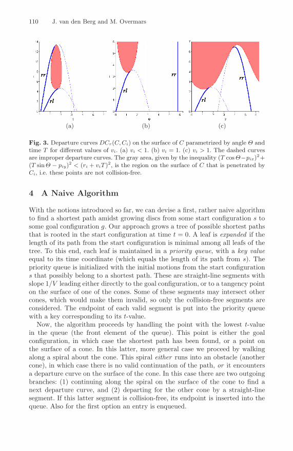
Here, D(T, Θ) is the discriminant whose sign indicates whether or not line �intersects Ci. When D(T, Θ) = 0, � is tangent to Ci, hence D(T, Θ) = 0 is animplicit equation for the set DCr(C, Ci). We can make this explicit by solvingD(T, Θ) = 0 for T . In Fig. 3 this function is plotted for various values of vi (notethat the function has a period of 2π). In each of these cases we see two sine-like curves (for vi = 1, it is degenerate). They correspond with DCrl(C, Ci)and DCrr(C, Ci), respectively. The other departure curves DClr(C, Ci) andDCll(C, Ci) can be found when considering clockwise spirals.

Given a position (T, Θ) on the surface of cone C for which D(T, Θ) = 0,the arrival time of the straight-line segment at cone Ci is given by A(T, Θ).The departure time of the segment is given by T . For some points along thedeparture curve A(T, Θ) is smaller than T . They correspond with bitangenciesin the negative direction, i.e. the arrival time on Ci is smaller than the departuretime at C. In the plots this is indicated by dashed curves. In the remainder ofthis paper these improper curves are ignored when we refer to departure curves.

We also have to take into account departure curves of DC(C, g) associatedwith segments tangent to C and leading to the goal configuration g. In this case,we have to solve the system of equations [�(t) = g] for T , to get a closed formfor the departure curve.

110 J. van den Berg and M. Overmars

(a) (b) (c)

Fig. 3. Departure curves DCr(C,Ci) on the surface of C parametrized by angle Θ andtime T for different values of vi. (a) vi < 1. (b) vi = 1. (c) vi > 1. The dashed curvesare improper departure curves. The gray area, given by the inequality (T cos Θ−pix)2+(T sin Θ − piy)2 < (ri + viT )2, is the region on the surface of C that is penetrated byCi, i.e. these points are not collision-free.

4 A Naive Algorithm

With the notions introduced so far, we can devise a first, rather naive algorithmto find a shortest path amidst growing discs from some start configuration s tosome goal configuration g. Our approach grows a tree of possible shortest pathsthat is rooted in the start configuration at time t = 0. A leaf is expanded if thelength of its path from the start configuration is minimal among all leafs of thetree. To this end, each leaf is maintained in a priority queue, with a key valueequal to its time coordinate (which equals the length of its path from s). Thepriority queue is initialized with the initial motions from the start configurations that possibly belong to a shortest path. These are straight-line segments withslope 1/V leading either directly to the goal configuration, or to a tangency pointon the surface of one of the cones. Some of these segments may intersect othercones, which would make them invalid, so only the collision-free segments areconsidered. The endpoint of each valid segment is put into the priority queuewith a key corresponding to its t-value.

Now, the algorithm proceeds by handling the point with the lowest t-valuein the queue (the front element of the queue). This point is either the goalconfiguration, in which case the shortest path has been found, or a point onthe surface of a cone. In this latter, more general case we proceed by walkingalong a spiral about the cone. This spiral either runs into an obstacle (anothercone), in which case there is no valid continuation of the path, or it encountersa departure curve on the surface of the cone. In this case there are two outgoingbranches: (1) continuing along the spiral on the surface of the cone to find anext departure curve, and (2) departing for the other cone by a straight-linesegment. If this latter segment is collision-free, its endpoint is inserted into thequeue. Also for the first option an entry is enqueued.

Planning the Shortest Safe Path Amidst Unpredictably Moving Obstacles 111

This procedure is repeated until the goal configuration is popped from thepriority queue. In this case the shortest path has been found, and can be readout if backpointers have been maintained during the algorithm. If the priorityqueue becomes empty, or if the front element of the queue has a time-value forwhich the goal configuration is not collision-free anymore (it is occupied by oneof the growing discs), no valid path exists. In Algorithm 1, the algorithm is givenin pseudocode.

Algorithm 1. ShortestPathNaive(s, g)1: Initialize priority queue Q with endpoints of all valid outgoing segments from s.2: while Q is not empty do3: Pop the front element 〈q, t〉 from the queue.4: if the goal configuration is not collision-free anymore at time t then5: Path does not exist. Terminate.6: else if q = g then7: Shortest path found! Terminate.8: else9: q is on the surface of a cone, say Ci, so proceed along the spiral about Ci until

it runs into another cone, or encounters a departure curve.10: if the spiral encounters a departure curve, say DC(Ci, Cj), then11: 〈q′, t′〉 ← the intersection point of the spiral and the departure curve.12: 〈q′′, t′′〉 ← arrival point of the bitangent segment on the surface of Cj .13: Insert 〈q′, t′〉 into Q.14: if segment 〈q′, t′〉, 〈q′′, t′′〉 is collision-free then15: Insert 〈q′′, t′′〉 into Q.16: Path does not exist.

In the above algorithm, we have to identify the spiral we are on (let us assumethat it is a counterclockwise spiral), given a point on the surface of the cone(line 9). Let q be a point on the surface of some cone, say Ci, given in Euclideancoordinates (x, y, t). Then the corresponding coordinates (T, Θ) on the surfaceof Ci are given by (T, Θ) = (t, arctan y−piy

x−pix).

The spiral on the surface of Ci going through (T, Θ) is given by θ0 as computedin Equation (6). Equation (5) then gives a function for the angle θ(t) alongthe spiral through (T, Θ). In line 10 of Algorithm 1, we wish to know whetherthe spiral encounters any departure curves. To this end, we should find theintersections of the spiral and the departure curves on the surface of Ci. Recallthat we can deduce an implicit equation D(T, Θ) = 0 for the departure curves ofany pair of cones (see Equation (8)). The intersections are thus found by solvingD(t, θ(t)) = 0 for t.

When we have found an intersection for some value t = T of the spiral anda departure curve of, say, DC(Ci, Cj), we wish to know what kind of departurecurve we have encountered. The arrival time at cone Cj when departed fromtime T is A(T, θ(T )) (see Equation (8)). If this arrival time is smaller than T ,the intersection can be ignored. If it is larger, we like to know whether the tangent

112 J. van den Berg and M. Overmars

straight-line segment arrives on the left side of Cj (and should be succeeded bya clockwise spiral on Cj), or on the right side of Cj (and should be succeededby a counterclockwise spiral). This is determined by the derivative of D(t, θ(t))to t. If this derivative is negative at point T , we have arrived on the left side.If it is positive, we have arrived on the right side. The exact arrival location onthe surface of cone Cj is given by �(A(T, θ(T )) (see Equation (7)). From thisinformation we can deduce the parameters defining the spiral on Cj on whichwe have arrived.

5 An Efficient Algorithm

The algorithm described above will indeed find a shortest path to the goal withina finite amount of time. However, in order to have a bound on the running timewe must define nodes that can provably be visited only once in a shortest path,such that we can do relaxation on them as in Dijkstra’s algorithm [7]. We willshow that this is easy to achieve in the restricted case where all discs have equalgrowth rates, and present an O(n3 log n) algorithm (n being the number of discs).For the general case this problem is left open, but we will present an algorithmthat is very fast in practice, by pruning large parts of the search tree.

5.1 Discs with Equal Growth Rates

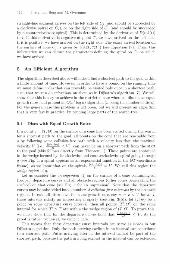
If a point q = (T, Θ) on the surface of a cone has been visited during the searchfor a shortest path to the goal, all points on the cone that are reachable fromq by following some collision-free path with a velocity less than the maximalvelocity V (i.e., ‖(δx,δy)‖

δt < V ), can never lie on a shortest path from the startto the goal (this follows directly from Theorem 1). These points are containedin the wedge formed by the clockwise and counterclockwise spiral going throughq (see Fig. 4; a spiral appears as an exponential function in the ΘT -coordinateframe), as we know that on the spirals ‖(δx,δy)‖

δt = V . We call this region thewedge region of q.

Let us consider the arrangement [1] on the surface of a cone containing all(proper) departure curves and all obstacle regions (other cones penetrating thesurface) on that cone (see Fig. 5 for an impression). Note that the departurecurves may be subdivided into a number of collision-free intervals by the obstacleregions. In case all discs have the same growth rate, say vi = v < V for all i,these intervals satisfy an interesting property (see Fig. 3(b)): let (T, Θ) be apoint on some departure curve interval, then all points (T ′, Θ′) on the sameinterval for which T ′ > T are within the wedge region of (T, Θ). To prove this,we must show that for the departure curves hold that ‖(δx,δy)‖

δt ≤ V . As theproof is rather technical, we omit it here.

This means that these departure curve intervals can serve as nodes in ourDijkstra-algorithm. Only the path arriving earliest in an interval can contributeto a shortest path. Paths arriving later in the interval cannot be part of theshortest path, because the path arriving earliest in the interval can be extended

Planning the Shortest Safe Path Amidst Unpredictably Moving Obstacles 113

with a traversal along the interval to end up at the same position (and time) asthe path arriving later in the interval.

Fig. 4. The region (light grey)on the surface of a cone that isreachable from point q by pathswith ‖(δx,δy)‖

δt≤ V . The dark

grey area is an obstacle.

Each node (an interval) has two outgoingedges. Let the interval be a segment of a depar-ture curve of DC(Ci, Cj), then the first edge isa spiral segment to the next departure curve onthe surface of Ci, and the second edge consistsof a bitangent straight-line segment and a spiralsegment and arrives in the first departure curveencountered on the surface of Cj . For the firstedge, which stays on the cone, we have to deter-mine the next departure curve that is encoun-tered if we proceed by moving along the spiralabout the cone. This can be done efficiently usingthe arrangement, if we have computed its trape-zoidal map [1], where the sides of the trapezoidsare spiral segments.

For the second edge, which traverses to an-other cone, we have to determine what the firstdeparture curve is we will encounter there. Thiscan be done efficiently using the arrangement we have computed on that cone.Using a point-location query, we can determine in what cell of the arrangementthe straight-line segment has arrived, and using the trapezoidal map we knowwhat the first departure curve is we will encounter if we proceed from there.

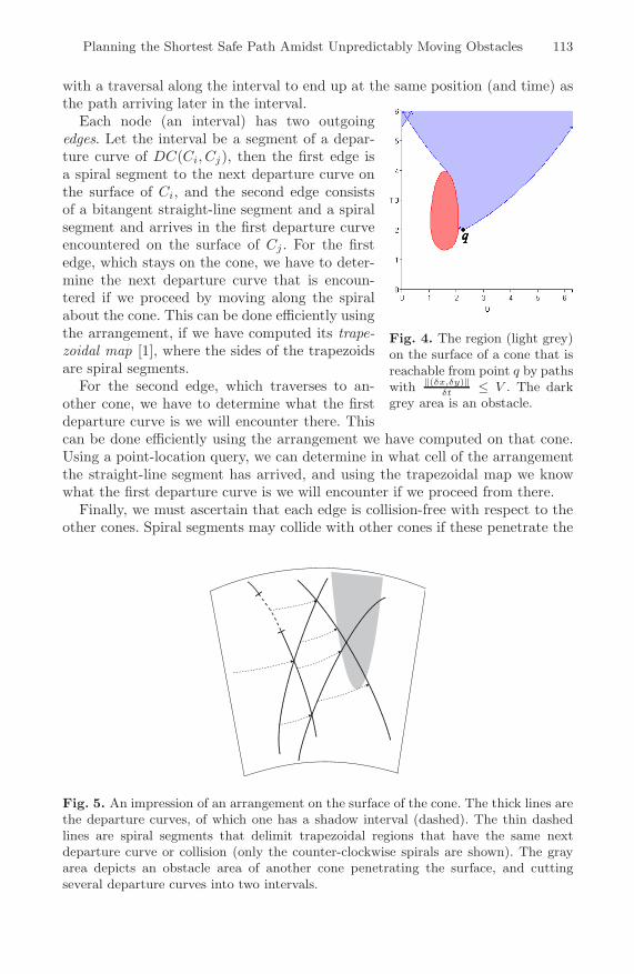
Finally, we must ascertain that each edge is collision-free with respect to theother cones. Spiral segments may collide with other cones if these penetrate the

Fig. 5. An impression of an arrangement on the surface of the cone. The thick lines arethe departure curves, of which one has a shadow interval (dashed). The thin dashedlines are spiral segments that delimit trapezoidal regions that have the same nextdeparture curve or collision (only the counter-clockwise spirals are shown). The grayarea depicts an obstacle area of another cone penetrating the surface, and cuttingseveral departure curves into two intervals.

114 J. van den Berg and M. Overmars

spiral’s cone surface. Since obstacle areas are incorporated into the arrangement,such collisions are easily detected. Straight-line segments may collide with anycone, so for each departure curve and each cone, we calculate the shadow inter-val this cone casts on the departure curve, in which a departure will result incollision. These shadow intervals are stored in the arrangement as well. In Fig. 5,an impression is given of how such an arrangement might look.

Theorem 4. The algorithm to compute a shortest path amidst n growing discswith equal growth rates runs in O(n3 log n) time.

Proof. For each pair of cones there are O(1) departure curves. Since there areO(n2) pairs of cones, there are O(n2) departure curves in total. Each of thedeparture curves can be segmented into at most O(n) intervals, as there areat most O(n) cones intersecting the departure curve (each cone can split thedeparture curve into at most two segments). Hence, there are O(n3) departurecurve intervals. Each departure curve interval has O(1) outgoing edges, makinga total of O(n3) edges.

The complexity of Dijkstra’s algorithm is known to be O(N log N +E) whereN is the number of nodes, and E the number of edges. Each edge requires someadditional work. Firstly, we have to find the departure curve interval in which itwill arrive, by doing a point-location query in the trapezoidal map of one of thearrangements. This takes O(log n) time. Further, we must determine whether anedge is collision-free. Using the shadow intervals stored at the departure curves,this can be done in O(log n) time as well. Thus, as both N and E are O(n3),Dijkstra’s algorithm will run in O(n3 log n) time in total.

Computing the arrangements and their trapezoidal maps takes O(n2) time percone, as there are O(n) departure curves on each cone, and O(n) intersectionareas of other cones. As there are O(n) cones, this step takes O(n3) time in total.All the shadow intervals can be computed in O(n3) time as well, as there areO(n2) departure curves and O(n) cones.

Overall, we can conclude that our algorithm runs in O(n3 log n) time. �

5.2 General Case: Discs Have Different Growth Rates

In the general case, where the discs may have different growth rates, the problembecomes much harder. We can follow the same approach as above, but let uslook at what happens to the slope of the departure curves in this case (see Figs.3(a) and (c)). In the case where the arrival cone has a slower growth rate, thedeparture curves (provably) satisfy ‖(δx,δy)‖

δt ≤ V (see Fig. 3(a)). However, in thecase where the arrival cone has a faster growth rate (Fig. 3(c)), it is clear that thisis not the case. The departure curve DCrr is horizontal at some point, meaningthat ‖(δx,δy)‖

δt = ∞. Hence, we cannot define intervals on these departure curvesthat serve as nodes in the search process.

We can still use Algorithm 1 for the general case, but a problem is thatthis algorithm considers many branches in the search tree of which we know

Planning the Shortest Safe Path Amidst Unpredictably Moving Obstacles 115

that they will not lead to a shortest path. For instance, it lets the spirals windaround the cones forever, thereby encountering many departure curves, which inturn generate other spirals on other cones. Hence, it lets the size of the searchtree blow up quickly.

In order to have an algorithm that runs fast in practice, we need to prunethese useless branches of the search tree. The key observation we use for this isthat a point (T, Θ) on the surface of cone Ci cannot be part of shortest path if wehave visited (T ′, Θ) already (where T ′ < T ) and the vertical line segment on thesurface of the cone between (T ′, Θ) and (T, Θ) is collision-free. This is because(T, Θ) is then in the wedge region of (T ′, Θ) (note that the velocity ‖(δx,δy)‖

δtalong the vertical line segment equals vi < V ). Hence a spiral encountering(T, Θ) need not be expanded any further.

To implement this practically, we only do this test for a constant number ofΘ’s. To this end, we augment Algorithm 1 by choosing a small constant ε, anddrawing 2π

ε evenly distributed vertical lines on the surface of each cone. Thesevertical lines are segmented into collision-free intervals by obstacle regions onthe surface. Now, these intervals will serve as nodes in our practical algorithmon which we perform relaxation.

This means that if we walk along a spiral on the surface of a cone, and thespiral crosses a vertical line, we have to check whether this spiral is the first toarrive in the particular interval. If not, this spiral can never be part of a shortestpath, for the same reasons as above. Thus, this branch of the search tree can bepruned.

The smaller ε is chosen, the sooner the spirals can be pruned, and hencethe smaller the size of the search tree will be. On the other hand, a smallerε also causes the algorithm to perform more (costly) relaxation checks, withdiminishing returns. So ε should not be chosen too small. Even though we areunable to bound the running time of this algorithm in terms of the number ofdiscs (n) or the value of ε, it turns out to be very fast in practice, as we will seenext.

5.3 Implementation Details

We created a fast implementation of Algorithm 1, augmented with the pruningheuristic presented above. We did not create an arrangement of all vertical linesand all obstacle regions on each cone. This would take too much time. Instead, wemaintain for each vertical line m one time-value at which it was last visited, saytm. Given the order in which the points are considered in the priority queue, weknow that when a point q is popped from the queue, it has a higher time value thanany point previously considered. So, if point q lies on vertical line m, its time valueqt is larger than the time-value tm of the point previously considered on that line.If the line segment between tm and qt on m is collision-free, q is in a previouslyvisited interval, and hence this point is not expanded. However, if the vertical linesegment between these two points is not collision-free, point q is the first to arrivein a new interval, and its outgoing edges must be inserted into the priority queue.

116 J. van den Berg and M. Overmars

From this moment on, qt is set as the time value attached to the vertical line m,as we know that no point below qt will be considered anymore.

Outgoing edges of a point q on a vertical line segment are a spiral segmentto the next vertical line, and –in case this spiral segment crosses one or moredeparture curves– segments to vertical lines on other cones. In our implemen-tation, the intersection between spiral segments and departure curves is foundusing a combination of two approximate root-finding algorithms [3].

Collision-checking straight-line segments is done by testing them for inter-sections with all cones, except the ones they are tangent to. We approximatea spiral segment between two consecutive vertical lines by one or more smallstraight-line segments, and collision-check them in the same way (in our imple-mentation, we use a single straight-line segment, as the radial distance ε betweentwo consecutive vertical lines is small).

Finally, the Dijkstra paradigm was replaced by an equally suited A*-method[7], that is faster in practice as it focusses the search to the goal. It adds a lowerbound estimate of the distance to the goal to the key-value of each point in thepriority queue. In our implementation, the lower bound estimate is simply theEuclidean distance divided by the maximal velocity.

6 Experimental Results

We created an interactive application for planning paths amidst growing discs.The properties of the growing discs (position, size, growth rate) can be changedby the user, and on-the-fly a new path is computed. From this application wereport results. Experiments were run on a Pentium IV 3.0GHz with 1 GByte ofmemory. The value of ε was optimized and fixed at 2π

40 .

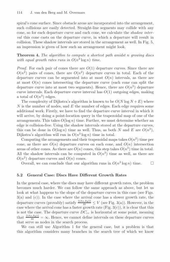
Fig. 6. A shortest path amidst 10 growing discs. A small dot indicates the positionalong the path at t = 0, 1, . . . , 7. The pictures were generated by our application.

Planning the Shortest Safe Path Amidst Unpredictably Moving Obstacles 117

We report the running times of the algorithm for a varying number of discs.As the running time of the algorithm does not only depend on the number ofobstacles, but also on the exact configuration of the discs, and how well the A*method manages to focus the search, etc., we averaged the running times overvarious positions of the start configuration for each experiment. In Fig. 7 theresults are given.

0

0.001

0.002

0.003

0.004

0.005

1 2 3 4 5 6 7 8 9 10 11 12 13 14 15

Number of discs

Run

ning

tim

e (s

)

Fig. 7. Results of our experiments

What first of all can be seenfrom the results is that our im-plementation is very fast. Even for15 growing discs, the running timeis only 0.0042 seconds, well withinreal-time requirements. We did notshow results for more than 15 discs,as it appeared to be difficult to findsensible setups with this many discsthat still contain a valid path to thegoal. From the figure it seems thatthe running time is more or lessquadratically related to the num-ber of discs. This is what we expected based on the implementation. In Fig. 6,snapshots are shown of a shortest path amidst 10 growing discs.

7 Conclusion

In this paper we presented an algorithm for computing shortest paths (mini-mum time paths) amidst discs that grow over time. A growing disc can modelthe region that is guaranteed to contain a moving obstacle of which the maximalvelocity is given. Hence, using our algorithm, paths can be found that are guar-anteed to be collision-free in the future, regardless of the behavior of the movingobstacles. As the regions grow fast over time, a new path should be planned fromtime to time –based on newly acquired sensor data– to generate paths with moreappealing global characteristics. Our implementation shows that such paths canbe generated very quickly. A great advantage over other methods is that thisreplanning can be done safely. The old path that is still used during replanningis guaranteed to be collision-free. A requirement though, is that the robot has ahigher maximal velocity than any of the moving obstacles.

A drawback of the method we presented is that a path to the goal often doesnot exist. This occurs when the goal is covered by a growing disc before it can bereached. A solution to this problem would be to find the path that comes closestto the goal. It seems that this can easily be incorporated into our algorithm.Other possible extensions include allowing obstacles with different shapes (otherthan discs), and fixed obstacles in the environment, but they are still subject ofongoing research.

118 J. van den Berg and M. Overmars

References

1. de Berg, M., van Kreveld, M., Overmars, M., Schwarzkopf, O.: ComputationalGeometry, Algorithms and Applications, ch. 6 and 8, 2nd edn. Springer, Berlin,Heidelberg (2000)

2. van den Berg, J., Ferguson, D., Kuffner, J.: Anytime path planning and replanningin dynamic environments. In: Proc. IEEE Int. Conf. on Robotics and Automation(ICRA) (2006)

3. Burden, R.L., Faires, J.D.: Numerical analysis, ch.2, 7th edn. Brooks/Cole, PacificGrove (2001)

4. Chang, E.C., Choi, S.W., Kwon, D.Y., Park, H., Yap, C.K.: Shortest path amidstdisc obstacles is computable. In: Proc. Ann. Symposium on Computational Geom-etry (SoCG), pp. 116–125 (2005)

5. Fiorini, P., Shiller, Z.: Motion planning in dynamic environments using velocityobstacles. Int. J. of Robotics Research 17(7), 760–772 (1998)

6. Hsu, D., Kindel, R., Latombe, J., Rock, S.: Randomized kinodynamic motion plan-ning with moving obstacles. Int. J. of Robotics Research 21(3), 233–255 (2002)

7. LaValle, S.M.: Planning Algorithms, ch. 2. Cambridge University Press, New York(2006)

8. Mitchell, J.S.B.: Geometric shortest paths and network optimization. In: Handbookof Computational Geometry, pp. 633–701. Elsevier Science Publishers, Amsterdam(2000)

9. Petty, S., Fraichard, T.: Safe motion planning in dynamic environments. In: Proc.IEEE Int. Conf. on Intelligent Robots and Systems (IROS), pp. 3726–3731 (2005)

10. Vasquez, D., Large, F., Fraichard, T., Laugier, C.: High-speed autonomous navi-gation with motion prediction for unknown moving obstacles. In: Proc. IEEE Int.Conf. on Intelligent Robots and Systems (IROS), pp. 82–87 (2004)

11. Weisstein, E.W.: Logarithmic Spiral. In MathWorld – a Wolfram web resource,http://mathworld.wolfram.com/LogarithmicSpiral.html