Planning for Improving Throughput in Autonomous Intersection Management

Tsz-Chiu Au, Michael Quinlan, Nicu Stiurca, Jesse Zhu, Peter StoneDepartment of Computer ScienceThe University of Texas at Austin

1 University Station C0500Austin, Texas 78712-1188

{chiu,mquinlan,jzhu,nstiurca,pstone}@cs.utexas.edu

Abstract

The impressive results of the 2007 DARPA UrbanChallenge showed that fully autonomous vehicles aretechnologically feasible with current intelligent vehi-cle hardware. It is natural to ask how current trans-portation infrastructure can be improved when most ve-hicles are driven autonomously in the future. Dres-ner and Stone proposed a new intersection controlmechanism called Autonomous Intersection Manage-ment (AIM) and showed in simulation that intersec-tion control can be made more efficient than the tra-ditional control mechanisms such as traffic signals andstop signs. In this paper, we extend the study to the realworld by examining the relationship between the pre-cision of cars’ motion controllers and the efficiency ofthe intersection controller. First, we propose a planning-based motion controller that can reduce the chance thatautonomous vehicles stop before intersections. Second,we present a mixed reality simulation environment thatallowed an autonomous vehicle in the real world to in-teract with many virtual vehicles in the AIM simulator.Finally, we experimentally determine a feasible set ofparameters for the motion controllers in simulation soas to give a more accurate account of the behavior ofautonomous vehicles.

IntroductionRecent advances in intelligent vehicle technology suggestthat autonomous vehicles will become a reality in the nearfuture (Squatriglia 2010). However, today’s transporta-tion infrastructure does not utilize the full capacity of au-tonomous driving systems. Dresner and Stone proposed amultiagent systems approach to intersection management,and in particular describe a First Come, First Served (FCFS)policy for directing vehicles through an intersection (Dres-ner and Stone 2008). This approach has been shown, insimulation, to yield significant improvements in intersectionperformance over conventional intersection control mecha-nisms such as traffic signals and stop signs. Despite, or per-haps because of the impressive performance, questions areoften raised regarding its applicability to real autonomousvehicles. In this paper we take the first step to show that

Copyright c© 2010, Association for the Advancement of ArtificialIntelligence (www.aaai.org). All rights reserved.

a real autonomous vehicle can adhere to the FCFS protocoland efficiently traverse an intersection.

In achieving this first step, we have obtained more accu-rate details regarding real-world parameters for future use insimulation. In particular we have confirmed that the noiseand imprecision of a real vehicle is greater than that antici-pated in the simulation. However, the FCFS algorithm wasdesigned with parameters (in the form of buffers) that canbe enlarged to account for these deficiencies. Even after theenlargement of these buffers we can still demonstrate thatFCFS provides a substantial performance improvement overthe four-way stop sign currently located at our test intersec-tion.

In addition, we believe that it is possible to make this in-tersection control mechanism more efficient by consideringhow best autonomous vehicles can utilize the FCFS pro-tocol. Armed with an increase in real-world knowledge,we leverage Little’s law in queueing theory to understandhow the performance of an autonomous vehicle relates tothe overall intersection throughput. Then we identify ap-proaches to improve the motion controllers of autonomousvehicles such that they can plan ahead of time when theymake reservations in the FCFS systems and traverse the in-tersection at a higher speed. We predict that the use of theseplanning techniques can improve the throughput of intersec-tions and reduce the traversal time of vehicles, thus pro-viding motivation for autonomous vehicles to adopt theseplanning-based controllers.

Autonomous Intersection ManagementTraffic signals and stop signs are very inefficient—not onlydo vehicles traversing intersections experience large de-lays, but the intersections themselves can only manage alimited traffic capacity—much less than that of the roadsthat feed into them. Dresner and Stone have introduced anovel approach to efficient intersection management that isa radical departure from existing traffic signal optimizationschemes (Dresner and Stone 2008). The solution is basedon a reservation paradigm, in which vehicles “call ahead” toreserve space-time in the intersection. In the approach, theyassume that computer programs called driver agents controlthe vehicles, while an arbiter agent called an intersectionmanager is placed at each intersection. The driver agentsattempt to reserve a block of space-time in the intersection.

The intersection manager decides whether to grant or rejectrequested reservations according to an intersection controlpolicy. In brief, the paradigm proceeds as follows.• An approaching vehicle announces its impending arrival

to the intersection manager. The vehicle indicates its size,predicted arrival time, velocity, acceleration, and arrivaland departure lanes.

• The intersection manager simulates the vehicle’s paththrough the intersection, checking for conflicts with thepaths of any previously processed vehicles.

• If there are no conflicts, the intersection manager issuesa reservation. It becomes the vehicle’s responsibility toarrive at, and travel through, the intersection as specified(within a range of error tolerance).

• The car may only enter the intersection once it has suc-cessfully obtained a reservation.Figure 1 diagrams the interaction between driver agents

and an intersection manager. A key feature of this paradigmis that it relies only on vehicle-to-infrastructure (V2I) com-munication. In particular, the vehicles need not know any-thing about each other beyond what is needed for local au-tonomous control (e.g., to avoid running into the car infront). The paradigm is also completely robust to commu-nication disruptions: if a message is dropped, either by theintersection manager or by the vehicle, delays may increase,but safety is not compromised. Safety can also be guaran-teed in mixed mode scenarios when both autonomous andmanual vehicles operate at intersections. The intersectionefficiency will increase with the ratio of autonomous vehi-cles to manual vehicles in such scenarios.

REQUEST

IntersectionControl Policy

REJECT

CONFIRM

Preprocess

Post

proc

ess

Yes,Restrictions

No, Reason

Driver

Agent

Intersection Manager

Figure 1: Diagram of the intersection system.

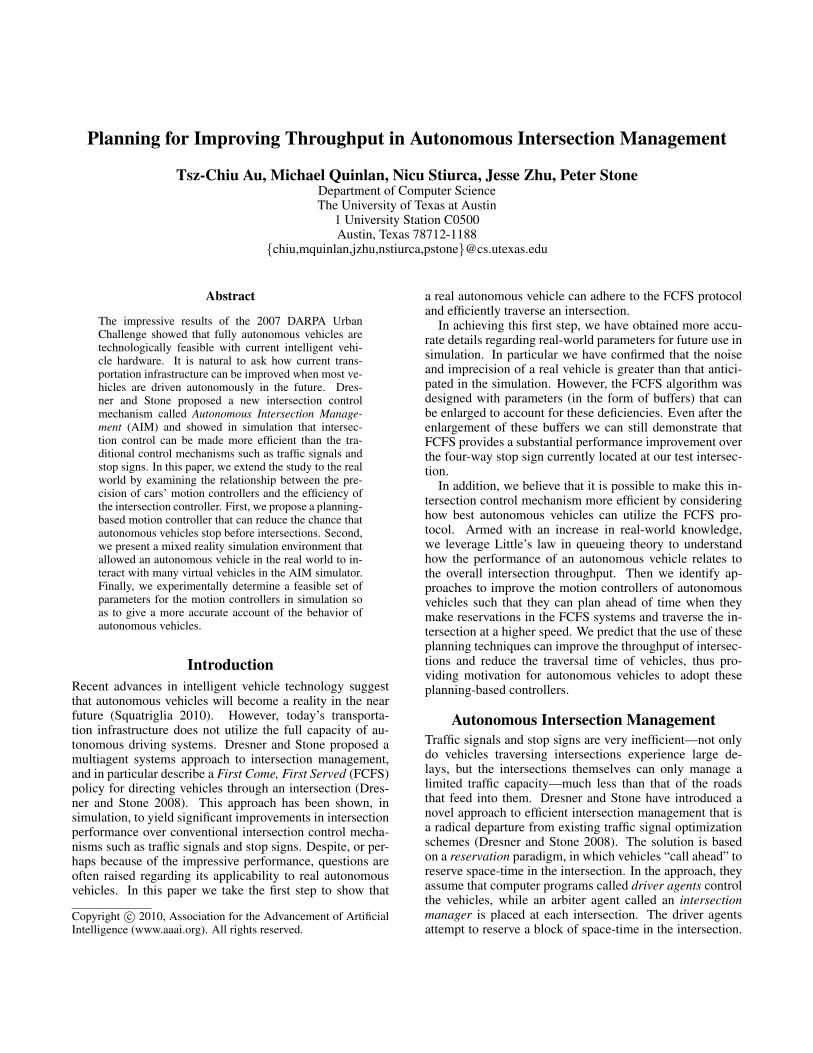
The prototype intersection control policy divides the inter-section into a grid of reservation tiles, as shown in Figure 2.When a vehicle approaches the intersection, the intersectionmanager uses the data in the reservation request regardingthe time and velocity of arrival, vehicle size, etc. to simulatethe intended journey across the intersection. At each simu-lated time step, the policy determines which reservation tileswill be occupied by the vehicle.

If at any time during the trajectory simulation the re-questing vehicle occupies a reservation tile that is alreadyreserved by another vehicle, the policy rejects the driver’sreservation request, and the intersection manager communi-cates this to the driver agent. Otherwise, the policy acceptsthe reservation and reserves the appropriate tiles. The inter-

(a) Successful (b) Rejected

Figure 2: (a) The vehicle’s space-time request has no con-flicts at time t. (b) The black vehicle’s request is rejectedbecause at time t of its simulated trajectory, the vehicle re-quires a tile already reserved by another vehicle. The shadedarea represents the static buffer of the vehicle.

section manager then sends a confirmation to the driver. Ifthe reservation is denied, it is the vehicle’s responsibility tomaintain a speed such that it can stop before the intersection.Meanwhile, it can request a different reservation.

Empirical results in simulation demonstrate that the pro-posed reservation system can dramatically improve the inter-section efficiency when compared to traditional intersectioncontrol mechanisms. To quantify efficiency, Dresner andStone introduce delay, defined as the amount of travel timeincurred by the vehicle as the result of passing through theintersection. According to their experiments, the reserva-tion system performs very well, nearly matching the perfor-mance of the optimal policy which represents a lower boundon delay should there be no other cars on the road (Figure 14in (Dresner and Stone 2008)). Overall, by allowing for muchfiner-grained coordination, the simulation-based reservationsystem can dramatically reduce per-car delay by two ordersof magnitude in comparison to traffic signals and stop signs.

Improving Throughput of Intersections viaPlanning Techniques

FCFS has been shown to be far more efficient than trafficlights and stop signs. But it is possible to make FCFS evenmore efficient by considering how autonomous vehicles canbetter utilize the FCFS protocol. In this section, we pro-pose some planning techniques to improve the motion con-troller of autonomous vehicles such that the traversal timeof the autonomous vehicles can be shortened and the overallthroughput of the intersection can be increased.

Little’s LawFirst of all, let us consider factors that affect the maximumthroughput characteristics of the FCFS protocol. An impor-tant result in queueing theory is Littles law (Little 1961),which states that in a queueing system the average arrivalrate of customers λ is equal to the average number of cus-tomers T in the system divided by the average time W acustomer spends in the system. In the context of intersec-tion management, Little’s law can be written as L = λW ,where

• L is the average number of vehicles in the intersection;• λ is the average arrival rate of the vehicles at the intersec-

tion; and• W is the average time a vehicle spends in the intersection.Note that the arrival rate is equal to the throughput of thesystem since no vehicle stalls inside an intersection.

Little’s law shows that the maximum throughput (i.e., theupper bound of λ) an intersection can sustain is equal to theupper bound of L divided by the lower bound of W , wherethe upper bound of L is the maximum number of vehiclesthat can coexist in an intersection, and the lower bound ofW is the minimum time a vehicle spends in the intersection.Thus, Little’s law shows that there are two ways to increasethe maximum throughput: 1) increase the average numberof vehicles in an intersection at any moment of time, and 2)decrease the average time a vehicle spends in an intersection.

A trivial upper bound on L is the area of the intersec-tion divided by the average static buffer size of the vehi-cles. But this bound is rather loose and in practice unachiev-able. Nonetheless, it provides us some hints that the max-imum throughput depends on the average static buffer sizeof the vehicles. But unfortunately the size of an intersec-tion is a hard limit and the static buffer sizes cannot be toosmall—that is, there is little an intersection manager can doto squeeze more vehicles into the intersection. Therefore,we have to consider the second way to increase the maxi-mum throughput.

Little’s law shows that by reducing the average timea vehicle takes to traverse an intersection, the maximumthroughput of the intersection can increase. In other words,a vehicle should maintain a high speed during the traversalof the intersection to shorten its traversal time. Vehicle’svelocity in the intersection depends on two factors: 1) theinitial velocity when the vehicle enters the intersection, and2) the acceleration during the traversal. In the following sec-tions, we will present two techniques that allow vehicles tomaintain a high speed during the traversal.

Planning for Making Reservations to AvoidStopping Before IntersectionsOne of the keys to entering an intersection at a high speed isto prevent vehicles from stopping before entering the inter-section. FCFS, by itself, reduces the number of vehicles thatstop at an intersection, and therefore it allows vehicles to en-ter an intersection at a high speed most of the time. In fact, itis one of the main reasons why FCFS is more efficient thantraffic lights and stop signs (Dresner and Stone 2008). WhileFCFS has done a good job in this regard, there is still roomfor improvement on the autonomous vehicles’ side such thatdriver agents can help by preventing themselves from stop-ping before an intersection.

There are two scenarios in which an autonomous vehiclehas to stop before an intersection in FCFS. First, the vehiclecannot obtain a reservation from the intersection managerand is forced to stop before an intersection. This happenswhen the traffic level is heavy and most of the future reser-vation tiles have been reserved by other vehicles in the sys-tem. Second, the vehicle successfully obtains a reservationbut later determines that it will not arrive at the intersection

at the time and/or velocity specified in the reservation. Inthis scenario the vehicle has to cancel the reservations andthose reservation tiles may have been wasted. The effectof a reservation cancellation is not only that the vehicle inquestion has to stop, but also that temporarily holding reser-vation tiles may have prevented another vehicle from mak-ing reservation. Both of these effects lead to a reduction inthe maximum throughput of the intersection.

A poor estimation of arrival times and arrival velocitiescan lead to the cancellation of reservations. In previouswork, the estimation of arrival times and arrival velocitiesis based on a heuristic we called the optimistic/pessimisticheuristic, that derives the arrival time and arrival velocitybased on a prediction about whether the vehicle can arriveat the intersection without the intervention of other vehi-cles (Dresner 2009). However, this heuristic presents noguarantee that the vehicle can arrive at the intersection atthe estimated arrival time or the estimated arrival velocity;in fact, experiments have shown that vehicles are often un-able to reach the intersection at the correct time and canceltheir reservations. To avoid this problem we propose a newway to estimate the arrival time and arrival velocity. In oursolution when a driver agent estimates its arrival time andarrival velocity, it also generates a sequence of control sig-nals. These control signals, if followed correctly, ensure thatthe vehicle will arrive at the estimated arrival time and at theestimated arrival velocity. We can formulate this estimationproblem as the following multiobjective optimization prob-lem: among all possible sequences of control signals thatcontrol the vehicle to enter an intersection, find one suchthat the arrival time is the smallest and the arrival velocity isthe highest.

For an acceleration-based controller, the sequence of con-trol signals is a time sequence of accelerations stating the ac-celeration the vehicle should take at every time step. We calla time sequence of accelerations an acceleration schedule.Like many multiobjective optimization problems, there isno single solution that dominates all other solutions in termsof both arrival time and arrival velocity. Here we choosearrival velocity as the primary objective, since a higher ar-rival velocity can allow the vehicle to enter the intersectionat a higher speed. Our optimization procedure involves twosteps: first, determine the highest possible arrival velocitythe vehicle can achieve, and second, among all the accelera-tion schedules that yield the highest possible arrival velocity,find the one whose arrival time is the soonest.

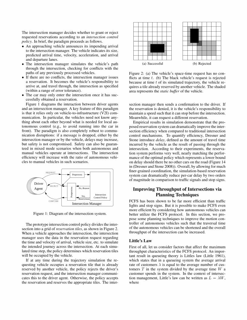
We illustrate how the estimation procedure works usinga time-velocity diagram as shown in Figure 3. In this fig-ure, v1 is the current velocity of the vehicle, t1 is the cur-rent time, D is the distance from the intersection, amax isthe maximum acceleration, amin is the minimum decelera-tion, vmax is the speed limit of the road, and vmax

2 is thespeed limit at the intersection. We can see that any functionv(·) in the time-velocity diagram that satisfies the follow-ing constraints is a feasible velocity schedule for reachingthe intersection, and the derivative of v(·) is an accelerationschedule for acceleration-based controller. (1) v(t1) = v1;(2) v(t) ≤ vmax for 0 ≤ t ≤ tend, where tend is the arrivaltime; (3) v(tend) ≤ vmax

2 ; (4) amin ≤ ddtv(t) ≤ amax for

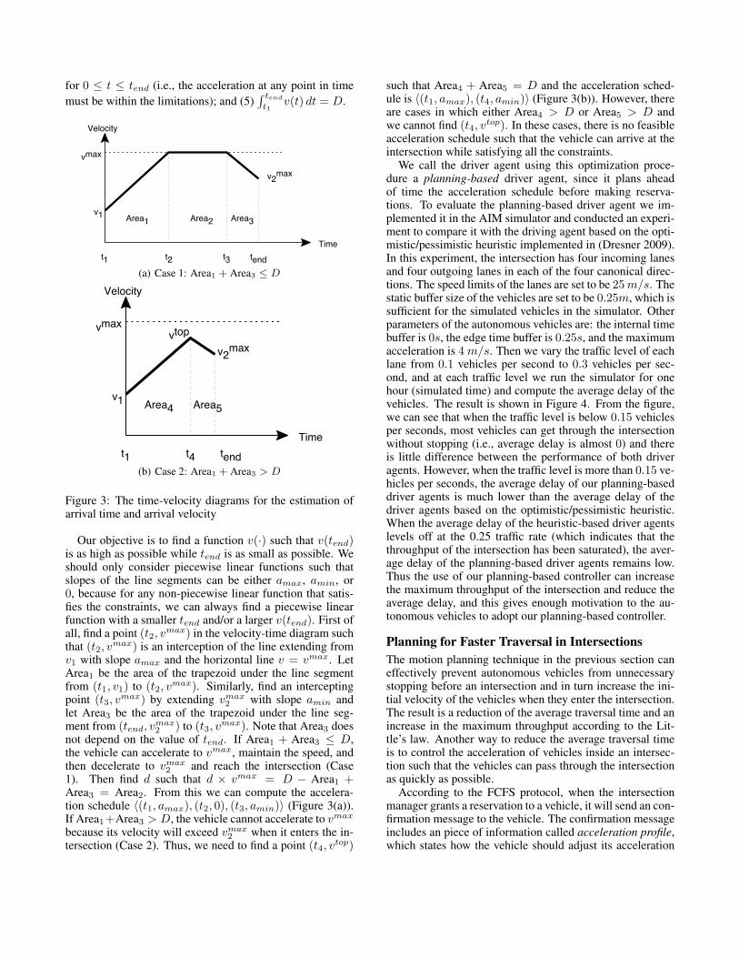
for 0 ≤ t ≤ tend (i.e., the acceleration at any point in timemust be within the limitations); and (5)

∫ tend

t1v(t) dt = D.

Velocity

Time

v1

v2max

vmax

Area1 Area2 Area3

t2 t3t1 tend(a) Case 1: Area1 + Area3 ≤ D

Velocity

Time

v1

v2max

vmax

Area4 Area5

vtop

t4t1 tend(b) Case 2: Area1 + Area3 > D

Figure 3: The time-velocity diagrams for the estimation ofarrival time and arrival velocity

Our objective is to find a function v(·) such that v(tend)is as high as possible while tend is as small as possible. Weshould only consider piecewise linear functions such thatslopes of the line segments can be either amax, amin, or0, because for any non-piecewise linear function that satis-fies the constraints, we can always find a piecewise linearfunction with a smaller tend and/or a larger v(tend). First ofall, find a point (t2, vmax) in the velocity-time diagram suchthat (t2, vmax) is an interception of the line extending fromv1 with slope amax and the horizontal line v = vmax. LetArea1 be the area of the trapezoid under the line segmentfrom (t1, v1) to (t2, vmax). Similarly, find an interceptingpoint (t3, vmax) by extending vmax

2 with slope amin andlet Area3 be the area of the trapezoid under the line seg-ment from (tend, v

max2 ) to (t3, vmax). Note that Area3 does

not depend on the value of tend. If Area1 + Area3 ≤ D,the vehicle can accelerate to vmax, maintain the speed, andthen decelerate to vmax

2 and reach the intersection (Case1). Then find d such that d × vmax = D − Area1 +Area3 = Area2. From this we can compute the accelera-tion schedule 〈(t1, amax), (t2, 0), (t3, amin)〉 (Figure 3(a)).If Area1+Area3 > D, the vehicle cannot accelerate to vmax

because its velocity will exceed vmax2 when it enters the in-

tersection (Case 2). Thus, we need to find a point (t4, vtop)

such that Area4 + Area5 = D and the acceleration sched-ule is 〈(t1, amax), (t4, amin)〉 (Figure 3(b)). However, thereare cases in which either Area4 > D or Area5 > D andwe cannot find (t4, vtop). In these cases, there is no feasibleacceleration schedule such that the vehicle can arrive at theintersection while satisfying all the constraints.

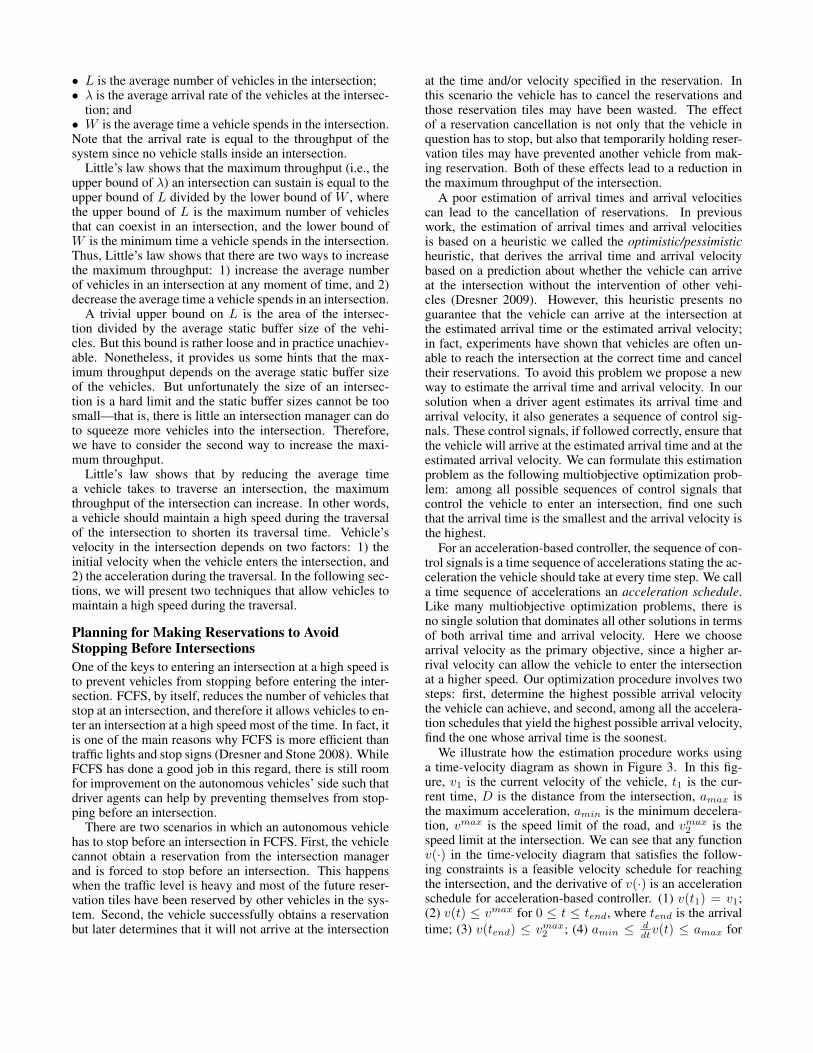
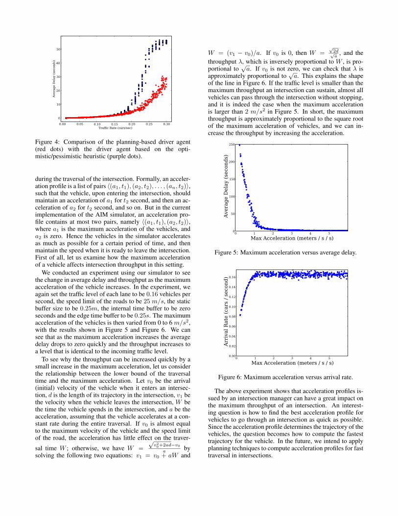
We call the driver agent using this optimization proce-dure a planning-based driver agent, since it plans aheadof time the acceleration schedule before making reserva-tions. To evaluate the planning-based driver agent we im-plemented it in the AIM simulator and conducted an experi-ment to compare it with the driving agent based on the opti-mistic/pessimistic heuristic implemented in (Dresner 2009).In this experiment, the intersection has four incoming lanesand four outgoing lanes in each of the four canonical direc-tions. The speed limits of the lanes are set to be 25 m/s. Thestatic buffer size of the vehicles are set to be 0.25m, which issufficient for the simulated vehicles in the simulator. Otherparameters of the autonomous vehicles are: the internal timebuffer is 0s, the edge time buffer is 0.25s, and the maximumacceleration is 4 m/s. Then we vary the traffic level of eachlane from 0.1 vehicles per second to 0.3 vehicles per sec-ond, and at each traffic level we run the simulator for onehour (simulated time) and compute the average delay of thevehicles. The result is shown in Figure 4. From the figure,we can see that when the traffic level is below 0.15 vehiclesper seconds, most vehicles can get through the intersectionwithout stopping (i.e., average delay is almost 0) and thereis little difference between the performance of both driveragents. However, when the traffic level is more than 0.15 ve-hicles per seconds, the average delay of our planning-baseddriver agents is much lower than the average delay of thedriver agents based on the optimistic/pessimistic heuristic.When the average delay of the heuristic-based driver agentslevels off at the 0.25 traffic rate (which indicates that thethroughput of the intersection has been saturated), the aver-age delay of the planning-based driver agents remains low.Thus the use of our planning-based controller can increasethe maximum throughput of the intersection and reduce theaverage delay, and this gives enough motivation to the au-tonomous vehicles to adopt our planning-based controller.

Planning for Faster Traversal in IntersectionsThe motion planning technique in the previous section caneffectively prevent autonomous vehicles from unnecessarystopping before an intersection and in turn increase the ini-tial velocity of the vehicles when they enter the intersection.The result is a reduction of the average traversal time and anincrease in the maximum throughput according to the Lit-tle’s law. Another way to reduce the average traversal timeis to control the acceleration of vehicles inside an intersec-tion such that the vehicles can pass through the intersectionas quickly as possible.

According to the FCFS protocol, when the intersectionmanager grants a reservation to a vehicle, it will send an con-firmation message to the vehicle. The confirmation messageincludes an piece of information called acceleration profile,which states how the vehicle should adjust its acceleration

0.00 0.05 0.10 0.15 0.20 0.25 0.30Traffic Rate (cars/sec)

0

10

20

30

40

50

Ave

rag

e D

ela

y (s

eco

nd

s)

Average Delay at Speed 7.5 m/s and Static Buffer size of 0.25

Figure 4: Comparison of the planning-based driver agent(red dots) with the driver agent based on the opti-mistic/pessimistic heuristic (purple dots).

during the traversal of the intersection. Formally, an acceler-ation profile is a list of pairs 〈(a1, t1), (a2, t2), . . . , (an, t2)〉,such that the vehicle, upon entering the intersection, shouldmaintain an acceleration of a1 for t2 second, and then an ac-celeration of a2 for t2 second, and so on. But in the currentimplementation of the AIM simulator, an acceleration pro-file contains at most two pairs, namely 〈(a1, t1), (a2, t2)〉,where a1 is the maximum acceleration of the vehicles, anda2 is zero. Hence the vehicles in the simulator acceleratesas much as possible for a certain period of time, and thenmaintain the speed when it is ready to leave the intersection.First of all, let us examine how the maximum accelerationof a vehicle affects intersection throughput in this setting.

We conducted an experiment using our simulator to seethe change in average delay and throughput as the maximumacceleration of the vehicle increases. In the experiment, weagain set the traffic level of each lane to be 0.16 vehicles persecond, the speed limit of the roads to be 25 m/s, the staticbuffer size to be 0.25m, the internal time buffer to be zeroseconds and the edge time buffer to be 0.25s. The maximumacceleration of the vehicles is then varied from 0 to 6 m/s2,with the results shown in Figure 5 and Figure 6. We cansee that as the maximum acceleration increases the averagedelay drops to zero quickly and the throughput increases toa level that is identical to the incoming traffic level.

To see why the throughput can be increased quickly by asmall increase in the maximum acceleration, let us considerthe relationship between the lower bound of the traversaltime and the maximum acceleration. Let v0 be the arrival(initial) velocity of the vehicle when it enters an intersec-tion, d is the length of its trajectory in the intersection, v1 bethe velocity when the vehicle leaves the intersection, W bethe time the vehicle spends in the intersection, and a be theacceleration, assuming that the vehicle accelerates at a con-stant rate during the entire traversal. If v0 is almost equalto the maximum velocity of the vehicle and the speed limitof the road, the acceleration has little effect on the traver-

sal time W ; otherwise, we have W =√

v20+2ad−v0

a bysolving the following two equations: v1 = v0 + aW and

W = (v1 − v0)/a. If v0 is 0, then W =√

2d√a

, and thethroughput λ, which is inversely proportional to W , is pro-portional to

√a. If v0 is not zero, we can check that λ is

approximately proportional to√

a. This explains the shapeof the line in Figure 6. If the traffic level is smaller than themaximum throughput an intersection can sustain, almost allvehicles can pass through the intersection without stopping,and it is indeed the case when the maximum accelerationis larger than 2 m/s2 in Figure 5. In short, the maximumthroughput is approximately proportional to the square rootof the maximum acceleration of vehicles, and we can in-crease the throughput by increasing the acceleration.

0 1 2 3 4 5

Max Acceleration (meters / s / s)

0

50

100

150

200

250

Ave

rag

e D

ela

y (s

eco

nd

s)

Figure 5: Maximum acceleration versus average delay.

0 1 2 3 4 5

Max Acceleration (meters / s / s)

0.00

0.02

0.04

0.06

0.08

0.10

0.12

0.14

0.16

Arr

ival

Rate

(ca

rs /

seco

nd

)

Figure 6: Maximum acceleration versus arrival rate.

The above experiment shows that acceleration profiles is-sued by an intersection manager can have a great impact onthe maximum throughput of an intersection. An interest-ing question is how to find the best acceleration profile forvehicles to go through an intersection as quick as possible.Since the acceleration profile determines the trajectory of thevehicles, the question becomes how to compute the fastesttrajectory for the vehicle. In the future, we intend to applyplanning techniques to compute acceleration profiles for fasttraversal in intersections.

Reality Check: AIM in PracticeSimulations inevitably will approximate critical aspects ofreality. For example, real cars may not be as preciselycontrollable as the simulated cars in simulations, nor mayGPS provide as reliable location estimates. The true testof the intersection management scheme will be how wellit works in the real-world, with real autonomous vehicles.In other words, in order to do realistic action planning forautonomous vehicles at intersections, we need to ground itwith realistic motion planning, and that needs to be verifiedin the real world.

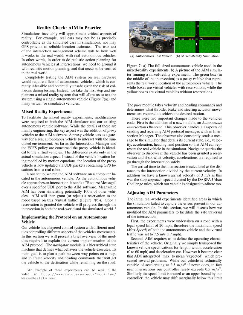
Completely testing the AIM system on real hardwarewould require a fleet of autonomous vehicles, which is cur-rently infeasible and potentially unsafe given the risk of col-lisions during testing. Instead, we take the first step and im-plement a mixed reality system that will allow us to test thesystem using a single autonomous vehicle (Figure 7(a)) andmany virtual (or simulated) vehicles.

Mixed Reality ExperimentsTo facilitate the mixed reality experiments, modificationswere required to both the AIM simulator and our existingautonomous vehicle software. While the details of these aremainly engineering, the key aspect was the addition of proxyvehicles to the AIM software. A proxy vehicle acts as a gate-way for a real autonomous vehicle to interact with the sim-ulated environment. As far as the Intersection Manager andthe FCFS policy are concerned the proxy vehicle is identi-cal to the virtual vehicles. The difference exists only in theactual simulation aspect. Instead of the vehicle location be-ing modelled by motion equations, the location of the proxyvehicle is now updated via UDP packets containing GPS lo-cations from a real robot.

In our setup, we ran the AIM software on a computer lo-cated in the autonomous vehicle. As the autonomous vehi-cle approaches an intersection, it sends a ”Request Message”over a specified UDP port to the AIM software. MeanwhileAIM has been simulating potentially 100’s of other vehi-cles. AIM will then grant (or reject) a reservation to therobot based on this ‘virtual traffic’ (Figure 7(b)). Once areservation is granted the vehicle will progress through theintersection in both the real-world and the simulated world. 1

Implementing the Protocol on an AutonomousVehicleOur vehicle has a layered control system with different mod-ules controlling different aspects of the vehicles movements.In this section we will present a brief overview of the mod-ules required to explain the current implementation of theAIM protocol. The navigator module is a hierarchical statemachine that defines what behavior the vehicle executes. Itsmain goal is to plan a path between way-points on a map,and to create velocity and heading commands that will getthe vehicle to the destination while remaining on the road.

1An example of these experiments can be seen in thevideo at http://www.cs.utexas.edu/∼mquinlan/MixedReality.wmv

(a) Autonomous Test Vehicle (b) Mixed-Reality Simulation

Figure 7: a) The full sized autonomous vehicle used in themixed-reality experiments. b) A picture of the AIM simula-tor running a mixed-reality experiment. The green box (inthe middle of the intersection) is a proxy vehicle that repre-sents the real world location of the autonomous vehicle. Thewhile boxes are virtual vehicles with reservations, while theyellow boxes are virtual vehicles without reservations.

The pilot module takes velocity and heading commands anddetermines what throttle, brake and steering actuator move-ments are required to achieve the desired motion.

There were two important changes made to the vehiclescode. First is the addition of a new module, an AutonomousIntersection Observer. This observer handles all aspects ofsending and receiving AIM protocol messages with an Inter-section Manager. The observer also constantly sends a mes-sage to the simulator that details its current state, i.e., veloc-ity, acceleration, heading, and position so that AIM can rep-resent the real vehicle in the simulator. Navigator queries theobserver to discover if the vehicle has been granted a reser-vation and if so, what velocity, accelerations are required togo through the intersection safely.

The arrival time to the intersection is calculated as the dis-tance to the intersection divided by the current velocity. Inaddition we have a known arrival velocity of 3 m/s as thiswas the stop-approach speed dictated by the DARPA UrbanChallenge rules, which our vehicle is designed to adhere too.

Adjusting AIM ParametersThe initial real-world experiments identified areas in whichthe simulation failed to capture the errors present in our au-tonomous vehicle. In this section, we will discuss how wemodified the AIM parameters to facilitate the safe traversalof the intersection.

First, the experiments were undertaken on a road with alegal speed limit of 20 mph, therefore the maximum speed(Max Speed) of both the autonomous vehicle and the virtualtraffic was set to 7.5 m/s (17 mph).

Second, AIM requires us to define the operating charac-teristics of the vehicle. Originally we simply transposed theknown vehicle specifications for length, width, acceleration(0 to 60 mph) and deceleration etc. However it became clearthat AIM interpreted ’max’ to mean ’expected’, which pre-sented several problems. While our vehicle is technicallycapable of accelerating at 2.5 m/s2 if never does, in factnear intersections our controller rarely exceeds 0.5 m/s2.Similarly the speed limit is treated as an upper bound by ourcontroller; the vehicle may drift marginally below this limit

for safety reasons and to facilitate smoother braking whenapproaching a stop.

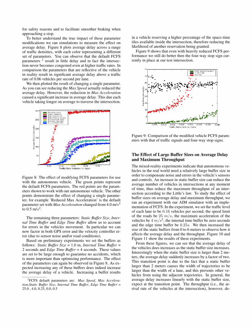
To better understand the true impact of these parametermodifications we ran simulations to measure the effect onaverage delay. Figure 8 plots average delay across a rangeof traffic densities, with each color representing a differentset of parameters. You can observe that the default FCFSparameters 2 result in little delay and in fact the intersec-tion never becomes congested even at higher traffic rates. Incomparison the parameters that are reflective of the vehiclein reality result in significant average delay above a trafficrate of 0.06 vehicles per second per lane.

We then plotted the result of changing a single parameter.As you can see reducing the Max Speed actually reduced theaverage delay. However, the reduction in Max Accelerationcaused a significant increase in average delay. This due eachvehicle taking longer on average to traverse the intersection.

Figure 8: The effect of modifying FCFS parameters for usewith the autonomous vehicle. The green points representthe default FCFS parameters. The red points are the param-eters shown to work with our autonomous vehicle. The otherpoints demonstrate the effect of changing a single parame-ter, for example ’Reduced Max Acceleration’ is the defaultparameter set with Max Acceleration changed from 4.0 m/s2

to 0.5 m/s2.

The remaining three parameters: Static Buffer Size, Inter-nal Time Buffer and Edge Time Buffer allow us to accountfor errors in the vehicles movement. In particular we cannow factor in both GPS error and the velocity controller er-ror (due to sensor noise and/or road conditions).

Based on preliminary experiments we set the buffers asfollows: Static Buffer Size = 1.0 m, Internal Time Buffer =2 seconds and Edge Time Buffer = 4 seconds. These valuesare set to be large enough to guarantee no accidents, whichis more important than optimizing performance. The effectof the parameters can again be observed in Figure 8. As ex-pected increasing any of these buffers does indeed increasethe average delay of a vehicle. Increasing a buffer results

2FCFS default parameters are: Max Speed, Max Accelera-tion,Static Buffer Size, Internal Time Buffer, Edge Time Buffer =25.0 , 4.0, 0.25, 0.0, 0.5

in a vehicle reserving a higher percentage of the space-timetiles available inside the intersection, therefore reducing thelikelihood of another reservation being granted.

Figure 9 shows that even with heavily reduced FCFS per-formance we still do better then the four-way stop sign cur-rently in place at our test intersection.

Figure 9: Comparison of the modified vehicle FCFS param-eters with that of traffic signals and four-way stop signs.

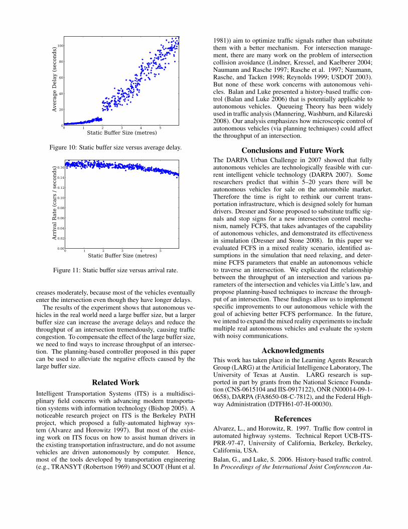
The Effect of Large Buffer Sizes on Average Delayand Maximum ThroughputThe mixed-reality experiments indicate that autonomous ve-hicles in the real world need a relatively large buffer size inorder to compensate noise and errors in the vehicle’s sensorsand controls. An increase in static buffer size can reduce theaverage number of vehicles in intersections at any momentof time, thus reduce the maximum throughput of an inter-section according to the Little’s law. To study the effect ofbuffer sizes on average delay and maximum throughput, weran an experiment with our AIM simulator with an imple-mentation of FCFS. In the experiment, we set the traffic levelof each lane to be 0.16 vehicles per second, the speed limitof the roads be 25 m/s, the maximum acceleration of thevehicles be 4 m/s2, the internal time buffer be zero secondsand the edge time buffer be 0.25s. We then increased thesize of the static buffers from 0 to 6 meters to observe how itaffects the average delay and the throughput. Figure 10 andFigure 11 show the results of these experiments.

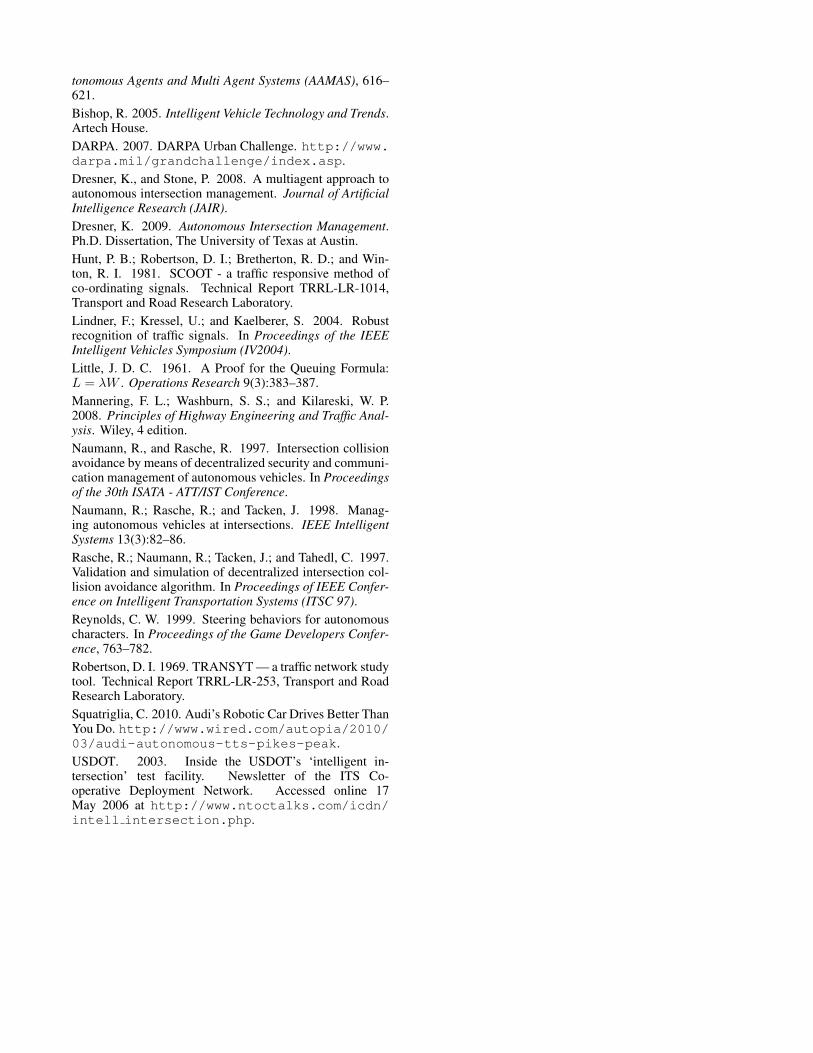
From these figures, we can see that the average delay ofthe vehicles does increases as the static buffer size increases.Interestingly when the static buffer size is larger than 2 me-ters, the average delay suddenly increases by a factor of two.This transition point is due to the fact that a static bufferlarger than 2 meters causes the width of trajectories to belarger than the width of a lane, and this prevents other ve-hicles from using the adjacent trajectories. In general, theaverage delay increases linearly with the static buffer size,expect at the transition point. The throughput (i.e., the ar-rival rate of the vehicles at the intersection), however, de-

0 1 2 3 4 5

Static Buffer Size (metres)

0

20

40

60

80

100

Ave

rag

e D

ela

y (s

eco

nd

s)

Figure 10: Static buffer size versus average delay.

0 1 2 3 4 5

Static Buffer Size (metres)

0.00

0.02

0.04

0.06

0.08

0.10

0.12

0.14

0.16

Arr

ival

Rate

(ca

rs /

seco

nd

s)

Figure 11: Static buffer size versus arrival rate.

creases moderately, because most of the vehicles eventuallyenter the intersection even though they have longer delays.

The results of the experiment shows that autonomous ve-hicles in the real world need a large buffer size, but a largerbuffer size can increase the average delays and reduce thethroughput of an intersection tremendously, causing trafficcongestion. To compensate the effect of the large buffer size,we need to find ways to increase throughput of an intersec-tion. The planning-based controller proposed in this papercan be used to alleviate the negative effects caused by thelarge buffer size.

Related WorkIntelligent Transportation Systems (ITS) is a multidisci-plinary field concerns with advancing modern transporta-tion systems with information technology (Bishop 2005). Anoticeable research project on ITS is the Berkeley PATHproject, which proposed a fully-automated highway sys-tem (Alvarez and Horowitz 1997). But most of the exist-ing work on ITS focus on how to assist human drivers inthe existing transportation infrastructure, and do not assumevehicles are driven autonomously by computer. Hence,most of the tools developed by transportation engineering(e.g., TRANSYT (Robertson 1969) and SCOOT (Hunt et al.

1981)) aim to optimize traffic signals rather than substitutethem with a better mechanism. For intersection manage-ment, there are many work on the problem of intersectioncollision avoidance (Lindner, Kressel, and Kaelberer 2004;Naumann and Rasche 1997; Rasche et al. 1997; Naumann,Rasche, and Tacken 1998; Reynolds 1999; USDOT 2003).But none of these work concerns with autonomous vehi-cles. Balan and Luke presented a history-based traffic con-trol (Balan and Luke 2006) that is potentially applicable toautonomous vehicles. Queueing Theory has been widelyused in traffic analysis (Mannering, Washburn, and Kilareski2008). Our analysis emphasizes how microscopic control ofautonomous vehicles (via planning techniques) could affectthe throughput of an intersection.

Conclusions and Future WorkThe DARPA Urban Challenge in 2007 showed that fullyautonomous vehicles are technologically feasible with cur-rent intelligent vehicle technology (DARPA 2007). Someresearchers predict that within 5–20 years there will beautonomous vehicles for sale on the automobile market.Therefore the time is right to rethink our current trans-portation infrastructure, which is designed solely for humandrivers. Dresner and Stone proposed to substitute traffic sig-nals and stop signs for a new intersection control mecha-nism, namely FCFS, that takes advantages of the capabilityof autonomous vehicles, and demonstrated its effectivenessin simulation (Dresner and Stone 2008). In this paper weevaluated FCFS in a mixed reality scenario, identified as-sumptions in the simulation that need relaxing, and deter-mine FCFS parameters that enable an autonomous vehicleto traverse an intersection. We explicated the relationshipbetween the throughput of an intersection and various pa-rameters of the intersection and vehicles via Little’s law, andpropose planning-based techniques to increase the through-put of an intersection. These findings allow us to implementspecific improvements to our autonomous vehicle with thegoal of achieving better FCFS performance. In the future,we intend to expand the mixed reality experiments to includemultiple real autonomous vehicles and evaluate the systemwith noisy communications.

AcknowledgmentsThis work has taken place in the Learning Agents ResearchGroup (LARG) at the Artificial Intelligence Laboratory, TheUniversity of Texas at Austin. LARG research is sup-ported in part by grants from the National Science Founda-tion (CNS-0615104 and IIS-0917122), ONR (N00014-09-1-0658), DARPA (FA8650-08-C-7812), and the Federal High-way Administration (DTFH61-07-H-00030).

ReferencesAlvarez, L., and Horowitz, R. 1997. Traffic flow control inautomated highway systems. Technical Report UCB-ITS-PRR-97-47, University of California, Berkeley, Berkeley,California, USA.Balan, G., and Luke, S. 2006. History-based traffic control.In Proceedings of the International Joint Conferenceon Au-

tonomous Agents and Multi Agent Systems (AAMAS), 616–621.Bishop, R. 2005. Intelligent Vehicle Technology and Trends.Artech House.DARPA. 2007. DARPA Urban Challenge. http://www.darpa.mil/grandchallenge/index.asp.Dresner, K., and Stone, P. 2008. A multiagent approach toautonomous intersection management. Journal of ArtificialIntelligence Research (JAIR).Dresner, K. 2009. Autonomous Intersection Management.Ph.D. Dissertation, The University of Texas at Austin.Hunt, P. B.; Robertson, D. I.; Bretherton, R. D.; and Win-ton, R. I. 1981. SCOOT - a traffic responsive method ofco-ordinating signals. Technical Report TRRL-LR-1014,Transport and Road Research Laboratory.Lindner, F.; Kressel, U.; and Kaelberer, S. 2004. Robustrecognition of traffic signals. In Proceedings of the IEEEIntelligent Vehicles Symposium (IV2004).Little, J. D. C. 1961. A Proof for the Queuing Formula:L = λW . Operations Research 9(3):383–387.Mannering, F. L.; Washburn, S. S.; and Kilareski, W. P.2008. Principles of Highway Engineering and Traffic Anal-ysis. Wiley, 4 edition.Naumann, R., and Rasche, R. 1997. Intersection collisionavoidance by means of decentralized security and communi-cation management of autonomous vehicles. In Proceedingsof the 30th ISATA - ATT/IST Conference.Naumann, R.; Rasche, R.; and Tacken, J. 1998. Manag-ing autonomous vehicles at intersections. IEEE IntelligentSystems 13(3):82–86.Rasche, R.; Naumann, R.; Tacken, J.; and Tahedl, C. 1997.Validation and simulation of decentralized intersection col-lision avoidance algorithm. In Proceedings of IEEE Confer-ence on Intelligent Transportation Systems (ITSC 97).Reynolds, C. W. 1999. Steering behaviors for autonomouscharacters. In Proceedings of the Game Developers Confer-ence, 763–782.Robertson, D. I. 1969. TRANSYT — a traffic network studytool. Technical Report TRRL-LR-253, Transport and RoadResearch Laboratory.Squatriglia, C. 2010. Audi’s Robotic Car Drives Better ThanYou Do. http://www.wired.com/autopia/2010/03/audi-autonomous-tts-pikes-peak.USDOT. 2003. Inside the USDOT’s ‘intelligent in-tersection’ test facility. Newsletter of the ITS Co-operative Deployment Network. Accessed online 17May 2006 at http://www.ntoctalks.com/icdn/intell intersection.php.