Planning Cost Estimates - Caltrans · October 31, 2008 1 1 Executive Summary The scope of this...
65
Planning Cost Estimates Project Report Divison of Design October 31, 2008
Transcript of Planning Cost Estimates - Caltrans · October 31, 2008 1 1 Executive Summary The scope of this...
Planning Cost Estimates
Project Report
Divison of Design
October 31, 2008

October 31, 2008
Table of Contents 1 Executive Summary............................................................................................................................................... 1
2 Purpose of the Report............................................................................................................................................ 3
3 Background ............................................................................................................................................................ 4 A HISTORY............................................................................................................................................................ 4 B DESCRIPTION..................................................................................................................................................... 6
(1) Problem Statement.................................................................................................................................. 6 (2) Overall Goal(s) ....................................................................................................................................... 6 (3) Outcome and Performance Measures..................................................................................................... 7
4 Overall Evaluation Goals ...................................................................................................................................... 7
5 Methodology........................................................................................................................................................... 7 A TYPES OF DATA/INFORMATION THAT WERE COLLECTED ................................................................................... 8 B HOW DATA/INFORMATION WERE COLLECTED AND ANALYZED.......................................................................... 8 C LIMITATIONS OF THE EVALUATION.................................................................................................................. 12
6 Interpretations and Conclusions ........................................................................................................................ 12 A ANALYSIS OF STATED COSTS ........................................................................................................................... 12 B ANALYSIS OF ESCALATED COSTS..................................................................................................................... 18
7 Recommendations................................................................................................................................................ 28 Appendices 1 IDC – Caltrans Committee Task Force No. 2 Final Report 2 Data Tables and Charts 3 District by District Comparison Charts 4 Cost Category Comparison Charts 5 PID Type Comparison Charts 6 Elapsed Time Comparison Charts

October 31, 2008 1
1 Executive Summary The scope of this study was to compare Planning Level Cost Estimates (Project Initiation Document (PID) Estimates) with subsequent Engineer’s Estimates (EE). In the final report for the Infrastructure Development Council (IDC) – Caltrans Committee Task Force on Cost Estimating, a measure was developed which defined an ”Acceptable” gap between the two estimates to be no more than 20 percent.
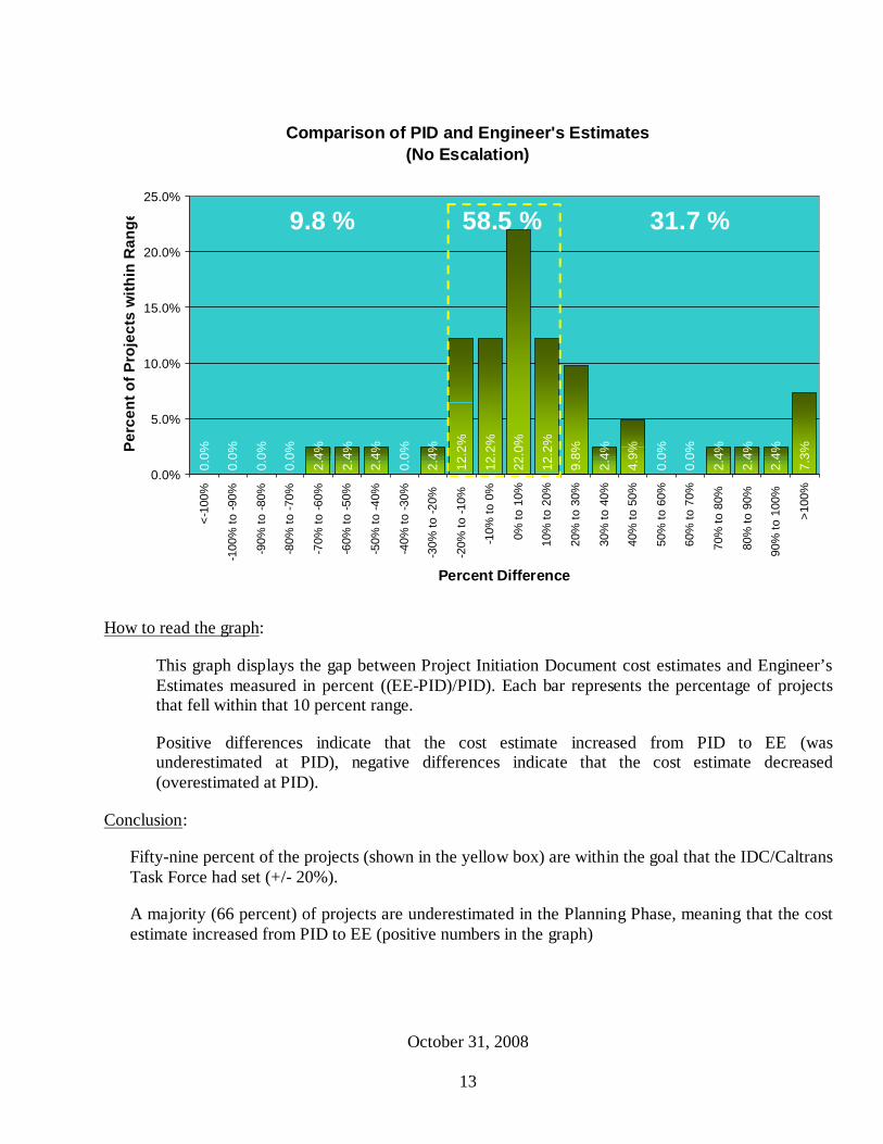
The histograms in Figures 1 and 2 below display the gap between Planning Level Cost Estimates and Engineer’s Estimates in percent and grouped in ranges of 10 percent from “< -100%” to “> 100%” for the sample projects. Positive numbers indicate that the PID cost estimate was underestimated, negative numbers indicate that the PID estimate was overestimated. The Y-axis (exact value displayed on each bar) indicates the percent of sample projects within each or range.
Figure 1 below displays the percent difference between non-escalated PID cost estimates and the subsequent Engineer’s Estimate. The Figure shows that 58.5 percent of the projects are within the goal set (+/- 20%).
Comparison of PID and Engineer's Estimates(No Escalation)
0.0%
0.0%
0.0%
0.0%
2.4%
2.4%
2.4%
0.0%
2.4%
12.2
%
12.2
%
22.0
%
12.2
%
9.8%
2.4%
4.9%
0.0%
0.0%
2.4%
2.4%
2.4%
7.3%
0.0%
5.0%
10.0%
15.0%
20.0%
25.0%
<-10
0%
-100
% to
-90%
-90%
to -8
0%
-80%
to -7
0%
-70%
to -6
0%
-60%
to -5
0%
-50%
to -4
0%
-40%
to -3
0%
-30%
to -2
0%
-20%
to -1
0%
-10%
to 0
%
0% to
10%
10%
to 2
0%
20%
to 3
0%
30%
to 4
0%
40%
to 5
0%
50%
to 6
0%
60%
to 7
0%
70%
to 8
0%
80%
to 9
0%
90%
to 1
00%
>100
%
Percent Difference
Perc
ent o
f Pro
ject
s w
ithin
Ran
ge 9.8 % 58.5 % 31.7 %
Figure 1: Comparison of PID and Engineer’s Estimates with no escalation
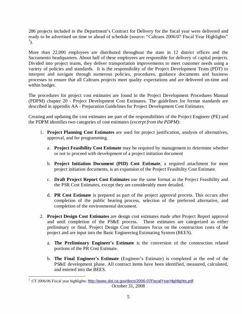
Table 1 below shows that 34.0 percent of the estimates were overestimated at the PID stage while 65.8 percent were underestimated.
October 31, 2008 2
Table 1: Data table for Figure 1 From To Count % From To Count % < -100% -100% 0 0% 100% > 100% 3 7.3% -100% -90% 0 0% 90% 100% 1 2.4% -90 % -80% 0 0% 80% 90% 1 2.4% -80% -70% 0 0% 70% 80% 1 2.4% -70% -60% 1 2.4% 60% 70% 0 0% -60% -50% 1 2.4% 50% 60% 0 0% -50% -40% 1 2.4% 40% 50% 2 4.9% -40% -30% 0 0% 30% 40% 1 2.4% -30% -20% 1 2.4% 20% 30% 4 9.8% -20% -10% 5 12.2% 10% 20% 5 12.2% -10% 0% 5 12.2% 0% 10% 9 22.0%
Overestimated 14 34.0% Underestimated 27 65.8%
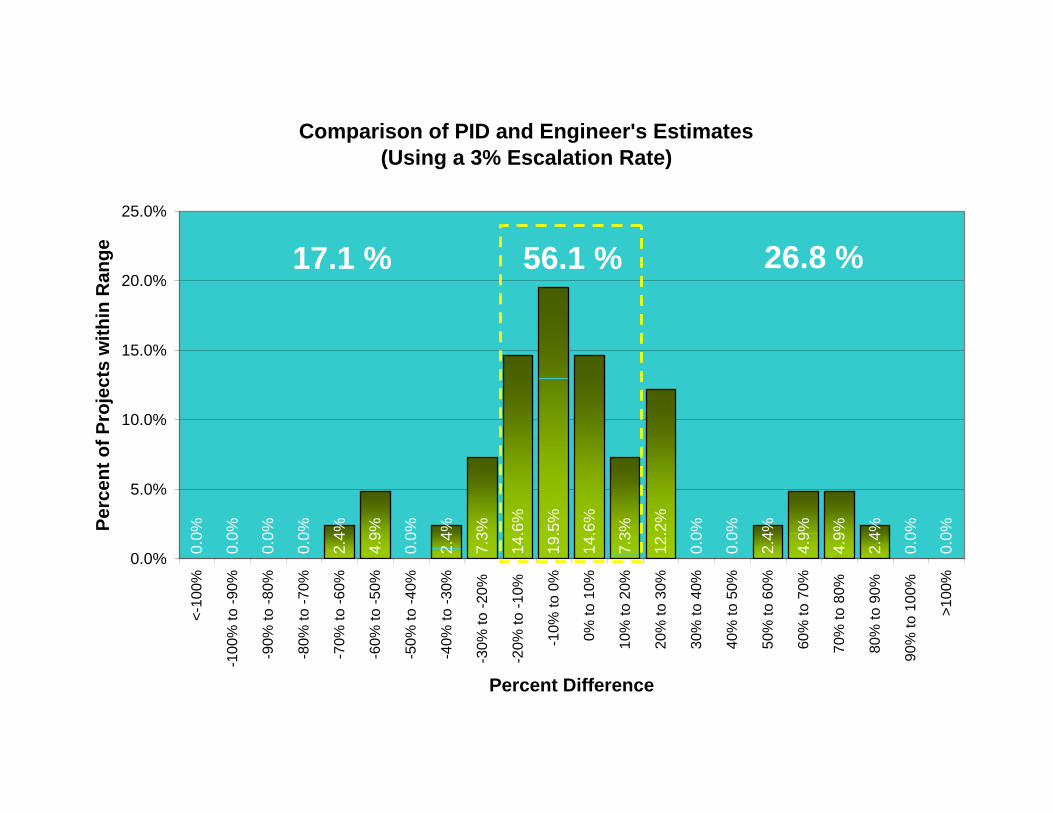
Figure 2 below is a similar histogram but this time the PID cost estimates are escalated using a three percent escalation rates. Historically, this was the rate used by Headquarters Programming to escalate project costs to the programming year. The graph shows that a lower proportion of projects, 56% are now within the goal set (+/- 20%).
Comparison of PID and Engineer's Estimates(Using a 3% Escalation Rate)
0.0%
0.0%
0.0%
0.0%
2.4%
4.9%
0.0%
2.4%
7.3%
14.6
%
19.5
%
14.6
%
7.3%
12.2
%
0.0%
0.0%
2.4%
4.9%
4.9%
2.4%
0.0%
0.0%
0.0%
5.0%
10.0%
15.0%
20.0%
25.0%
<-10
0%
-100
% to
-90%
-90%
to -8
0%
-80%
to -7
0%
-70%
to -6
0%
-60%
to -5
0%
-50%
to -4
0%
-40%
to -3
0%
-30%
to -2
0%
-20%
to -1
0%
-10%
to 0
%
0% to
10%
10%
to 2
0%
20%
to 3
0%
30%
to 4
0%
40%
to 5
0%
50%
to 6
0%
60%
to 7
0%
70%
to 8
0%
80%
to 9
0%
90%
to 1
00%
>100
%
Percent Difference
Perc
ent o
f Pro
ject
s w
ithin
Ran
ge 17.1 % 56.1 % 26.8 %
Figure 2: Comparison of PID and Engineer’s Estimates with escalation using a 3% escalation rate

October 31, 2008 3
Nearly the same number of projects fall within the desired range when using a three percent escalation rate as when there was there was no escalation. The primary difference is that fewer projects exceed the 120 percent overage that would require an increase in programming.
Table 1 below shows that when the PID Cost Estimates are escalated, 51.1 percent of the PID estimates were overestimated and 48.7 percent were underestimated.
Table 2: Data table for Figure 2 From To Count % From To Count % < -100% -100% 0 0% 100% > 100% 0 0% -100% -90% 0 0% 90% 100% 0 0% -90 % -80% 0 0% 80% 90% 1 2.4% -80% -70% 0 0% 70% 80% 2 4.9% -70% -60% 1 2.4% 60% 70% 2 4.9% -60% -50% 2 4.9% 50% 60% 1 2.4% -50% -40% 0 0.0% 40% 50% 0 0% -40% -30% 1 2.4% 30% 40% 0 0% -30% -20% 3 7.3% 20% 30% 5 12.2% -20% -10% 6 14.6% 10% 20% 3 7.3% -10% 0% 8 19.5% 0% 10% 6 14.6% Overestimated 21 51.1% Underestimated 20 48.7%
Other charts and tables were created to try to find any significant trends in the data specific to:
- Districts - Size of project (cost) - Time between PID and EE - PID Type
All graphs and explanations are included in Chapter 6 - Interpretations and Conclusions. No major trends were discovered in any of the categories. Some potential trends were noted and should be investigated further in a more detailed study, which could be included as the next step of this project.
The next step is to look at details within each cost estimate to try to identify any trends in what items or events led to the difference between the PID and Engineer’s Cost Estimates. The Department has decided to do this analysis in-house since it will require more extensive knowledge of projects and cost estimating processes.
2 Purpose of the Report This report contains the results of one stage of the cost estimate analysis process and the end of the phase performed by external consultants. This stage was developed to compare Project Initiation Document (PID) Estimates with Engineer’s Estimates to determine how well the Department is doing in achieving its goal of having these estimates fall within 20 percent of each other. The next step in this process is to perform detailed analysis and will be performed by Caltrans in-house staff.

October 31, 2008 4
In addition to this report, the consultant has delivered all documentation created during the project:
a. Project Initiation Document Estimate documents from all projects in the sample b. Engineer’s Estimate documents from some projects in the sample
c. Spreadsheets documenting and comparing costs from the two documents (per project)
3 Background This study was created as an element of the Quality Management project described in Caltrans Request For Offer QMP-002. The scope of the Quality Management project was to analyze the deployment and effectiveness of policies, procedures, standards with the ultimate goal being to help management improve the results of project delivery processes and the project results (cost, schedule, adherence to standards, and customer/stakeholder satisfaction).
The following policies/standards were selected for analysis:
A. Constructability policy
B. Cost estimating procedures
C. Landscaping Sight Distance and Clear Recovery Zone standards D. Safety of Highway planting standards & guidelines for maintainability
This report documents Project B – analysis of Cost Estimating procedures.
In 2006, the Infrastructure Development Council – Caltrans Committee formed Task Force No. 2 to investigate methods to improve the accuracy and level of confidence in project capital cost estimates. The task force met on a monthly basis between May 2006 and March 2007 to identify needed actions and to report back to the team on completed action items.
The task force developed the following expected goals (measures) for capital cost estimates:
• Planning level cost estimates are within 20 percent of subsequent Engineer’s Estimates
• Engineer’s Estimates at advertisement are within 10 percent of the low bid
• The final cost is within 5 percent of the awarded amount.
Caltrans currently collects data on the last two measures and can easily determine how well the Department is performing. The first measure is not currently being monitored and is the focus of this project.
A History Caltrans is an enormous project delivery organization and the fiscal year 2006/07 was historic with projects valued at more than $10 billion under construction, (not including Proposition 1B projects.) All
October 31, 2008 5
286 projects included in the Department’s Contract for Delivery for the fiscal year were delivered and ready to be advertised on time or ahead of schedule (source: “Caltrans 2006/07 Fiscal Year Highlights” 1).
More than 22,000 employees are distributed throughout the state in 12 district offices and the Sacramento headquarters. About half of these employees are responsible for delivery of capital projects. Divided into project teams, they deliver transportation improvements to meet customer needs using a variety of policies and standards. It is the responsibility of the Project Development Team (PDT) to interpret and navigate through numerous policies, procedures, guidance documents and business processes to ensure that all Caltrans projects meet quality expectations and are delivered on-time and within budget.
The procedures for project cost estimates are found in the Project Development Procedures Manual (PDPM) chapter 20 - Project Development Cost Estimates. The guidelines for format standards are described in appendix AA - Preparation Guidelines for Project Development Cost Estimates.
Creating and updating the cost estimates are part of the responsibilities of the Project Engineer (PE) and the PDPM identifies two categories of cost estimates (excerpt from the PDPM):
1. Project Planning Cost Estimates are used for project justification, analysis of alternatives, approval, and for programming.
a. Project Feasibility Cost Estimate may be required by management to determine whether or not to proceed with development of a project initiation document
b. Project Initiation Document (PID) Cost Estimate, a required attachment for most project initiation documents, is an expansion of the Project Feasibility Cost Estimate.
c. Draft Project Report Cost Estimates use the same format as the Project Feasibility and the PSR Cost Estimates, except they are considerably more detailed.
d. PR Cost Estimate is prepared as part of the project approval process. This occurs after completion of the public hearing process, selection of the preferred alternative, and completion of the environmental document.
2. Project Design Cost Estimates are design cost estimates made after Project Report approval and until completion of the PS&E process. These estimates are categorized as either preliminary or final. Project Design Cost Estimates focus on the construction costs of the project and are input into the Basic Engineering Estimating System (BEES).
a. The Preliminary Engineer's Estimate is the conversion of the construction related portions of the PR Cost Estimate.
b. The Final Engineer's Estimate (Engineer’s Estimate) is completed at the end of the PS&E development phase. All contract items have been identified, measured, calculated, and entered into the BEES.
1 CT 2006/06 Fiscal year highlights: http://www.dot.ca.gov/docs/2006-07FiscalYearHighlights.pdf

October 31, 2008 6
The two cost estimates included in this analysis are the PID Cost Estimate and the Engineer's Estimate.
B Description The original idea as described in QMP002 was to develop studies for measuring the effectiveness of the standards and policies, which for Cost Estimates would mean PDPM Chapter 20 and Appendix AA.
However, for cost estimates the work had already been started in 2006 by the IDC – Caltrans Committee Task Force No. 2. Instead of starting up a new project it was decided that this project would continue the work of this task force.
(1) Problem Statement
The final report by the IDC – Caltrans Committee Task Force No. 2 described the activities and conclusions from their work. One of their activities was the collection and monitoring of baseline data to measure cost estimating accuracy. The Task Force determined that the following was already being monitored:
• Caltrans Office Engineer produces a quarterly report comparing bid results to the Engineer’s Estimate as well as a report showing this same data for previous years. This information is now reported to Caltrans management on a regular basis.
• The cost growth during construction is tracked by Construction and is being reported to management.
They also found that PID baseline data was hard to obtain as Caltrans does not collect the data in a central database. In particular, they looked for an opportunity to track a comparison between planning level estimates and to Engineer’s Estimates, which ultimately led to the scope of this project.
(2) Overall Goal(s)
The IDC – Caltrans Committee Task Force No. 2 developed the following expected results (measures) for cost estimates:
1. Planning level cost estimates are within 20 percent of subsequent Engineer’s Estimates.
2. Engineer’s Estimates at advertisement are within 10 percent of the low bid
3. The final cost is within 5 percent of the awarded amount.
The specific goal of this project is to analyze a sample of actual projects to test measure number one: “Planning level cost estimates are within 20 percent of subsequent Engineer’s Estimates.”
October 31, 2008 7
(3) Outcome and Performance Measures
The importance of and procedures for quality cost estimates are laid out in the Project Development Procedures Manual (PDPM) Chapter 20 and Appendix AA. (The following texts are from these directives.)
The PDPM states that the reliability of project cost estimates at every stage in the project development process is necessary for responsible fiscal management.
“Unreliable cost estimates result in severe problems in Caltrans' programming and budgeting, in local and regional planning, and it results in staffing and budgeting decisions which could impair effective use of resources. This, in turn, affects Caltrans' relations with the California Transportation Commission (CTC), the Legislature, local and regional agencies, and the public, and results in loss of credibility.”
Caltrans' overall goal for a high quality management of costs is to avoid project cost overruns by identifying potential problems while they are still easy to change. Cost estimating is not an exact science but project engineers are helped by a comprehensive methodology and set of procedures to help guide them through the process. The problem is that the earlier an estimate is made, the more likely it is to change. It is hoped that this study comparing cost estimates at different stages of the process could possibly identify the items or areas that change the most and thus help in finding a solution for developing better cost estimates.
4 Overall Evaluation Goals The overall goal of this study was to assess the effectiveness of the project cost estimating process by using the following steps: (1) determine a meaningful process (measures, sample, etc.) for evaluating the gap between cost estimates in the project initiation document phase and the Engineers’ Estimate, (2) gather necessary project documents, and (3) perform a simple statistical analysis.
Recommendations are offered for future evaluation and technical assistance. All the cost estimates from the PID documents were copied and organized and submitted to Caltrans for use in further studies.
5 Methodology The projects included were selected through stratified sampling, a process where the distribution of projects within sub-populations are considered. (stratified sample: the population is divided into strata and a random sample is taken from each stratum. Ref: WordNet 3.0 2)
This project did not involve advanced statistical analysis so data was recorded and analyzed using an Microsoft Excel spreadsheet.
2 "Stratified sampling." WordNet 3.0 © Princeton University 2006 <http://wordnet.princeton.edu/perl/webwn?s=stratified+sample&o2=&o0=1&o7=&o5=&o1=1&o6=&o4=&o3=&h=>.

October 31, 2008 8
A Types of data/information that were collected The numbers to be included in the cost estimates developed over the time of the project due to the different formats of the PID estimates. The only items captured were Roadway Items and Structure Items, which combined were named Construction Costs.
Example: Initial table of included items:
Date EA County Route EE
7/24/01 01-292004 MEN 20 $5,086,708
Item Alt 1 Alt 2 Alt 3 Alt 4 Roadway Items $6,499,000.00 $7,051,000.00 $5,452,000.00 $4,540,000.00 Structure Items - - - -
Construction Cost $6,499,000.00 $7,051,000.00 $5,452,000.00 $4,540,000.00 Other - - - -
Total $6,499,000.00 $7,051,000.00 $5,452,000.00 $4,540,000.00
All project documents (PID estimates and Engineer’s Estimates) were copied and organized as they were collected. The following costs were captured (included in the spreadsheet) if included in the cost estimate, but were not used in the analysis.
1. R/W 2. R/W (Escalated) 3. Project Support Cost
All spreadsheets used to capture data are attached with this project report in Appendix
B How data/information was collected and analyzed The project team decided to draw a sample from all projects awarded during fiscal year 2006-07. The sampling process started on September 7, 2007 with a total of 652 projects with the following information.
BO Date Bid Opening Date EA Expenditure Authorization EE Engineer's Estimate Low Bid Lowest bid among bidding contractors % LB -EE Percent above or below Engineer's Estimate Number of Bidders How many contractors bid on this project Award Date Date the contract was awarded to the low bidder BO to Award Number of days between the bid opening date and the contract award
date
From the total population the following projects were removed:
October 31, 2008 9
• Projects that were split or combined with other projects (all projects with anything but a “0” in the second to last character in the EA)
• Projects with pending award or unaccepted bid (N/A in the award date column)
• Projects with EE under $1,000,000 (only major projects considered).
• Projects of such a character that PID documents are not required (e.g. emergency contracts and major maintenance).
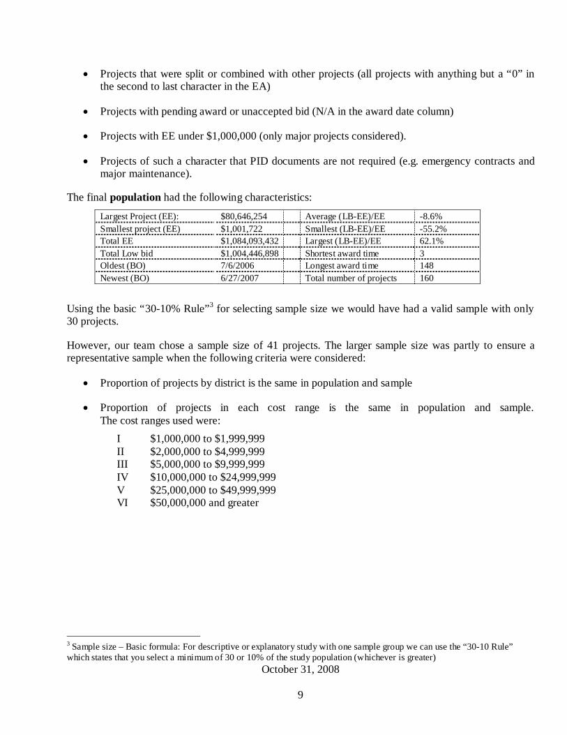
The final population had the following characteristics:
Largest Project (EE): $80,646,254 Average (LB-EE)/EE -8.6% Smallest project (EE) $1,001,722 Smallest (LB-EE)/EE -55.2% Total EE $1,084,093,432 Largest (LB-EE)/EE 62.1% Total Low bid $1,004,446,898 Shortest award time 3 Oldest (BO) 7/6/2006 Longest award time 148 Newest (BO) 6/27/2007 Total number of projects 160
Using the basic “30-10% Rule”3 for selecting sample size we would have had a valid sample with only 30 projects.
However, our team chose a sample size of 41 projects. The larger sample size was partly to ensure a representative sample when the following criteria were considered:
• Proportion of projects by district is the same in population and sample
• Proportion of projects in each cost range is the same in population and sample. The cost ranges used were:
I $1,000,000 to $1,999,999 II $2,000,000 to $4,999,999 III $5,000,000 to $9,999,999 IV $10,000,000 to $24,999,999 V $25,000,000 to $49,999,999 VI $50,000,000 and greater
3 Sample size – Basic formula: For descriptive or explanatory study with one sample group we can use the “30-10 Rule” which states that you select a minimum of 30 or 10% of the study population (whichever is greater)

October 31, 2008
10
The final population had the following cost range distribution per district:
Number of projects within cost range District Number of projects
% of total I II III IV V VI
District 1 11 7% 3 3 3 1 1 0 District 2 18 11% 9 4 4 0 1 0
District 3 16 10% 5 7 2 2 0 0 District 4 23 14% 3 9 3 4 2 2
District 5 7 4% 3 3 1 0 0 0 District 6 15 9% 6 5 2 1 0 1
District 7 19 12% 4 9 5 0 1 0 District 8 21 13% 4 10 3 3 1 0
District 9 2 1% 0 0 2 0 0 0 District 10 7 4% 1 3 1 1 1 0
District 11 12 7% 6 4 1 1 0 0 District 12 9 6% 1 3 2 3 0 0
Total 160 100% 46 60 29 16 7 3
The final sample had the following characteristics: Largest Project (EE): $19,460,842 Average (LB-EE)/EE -10.4% Smallest project (EE) $1,003,673 Smallest (LB-EE)/EE -47.0% Total EE $150,993,106 Largest (LB-EE)/EE 30.0% Total Low bid $129,299,762 Shortest award time 3 Oldest (BO) 7/6/2006 Longest award time 148 Newest (BO) 6/20/2007 # of projects in sample 41

October 31, 2008
11
The final sample had the following cost range distribution per district:
Number of projects within cost range District Number of projects
% of total I II III IV V VI
District 1 3 7% 2 0 1 0 0 0 District 2 5 12% 3 1 1 0 0 0
District 3 4 10% 2 2 0 0 0 0 District 4 5 12% 1 2 1 1 0 0
District 5 2 5% 1 1 0 0 0 0 District 6 3 7% 2 1 0 0 0 0
District 7 5 12% 2 2 1 0 0 0 District 8 6 15% 2 2 1 1 0 0
District 9 1 2% 0 0 1 0 0 0 District 10 1 2% 0 1 0 0 0 0
District 11 4 10% 3 1 0 0 0 0 District 12 2 5% 0 1 0 1 0 0
Total 41 100% 18 14 6 3
Note that with as few as one project in some districts our results should not be used to analyze trends for individual districts.
Document retrieval
To locate the project documents we used expenditure authorization numbers (EAs), route numbers and counties for each project to search through the project documents stored in the Headquarters Project Records Room. However, probably due to time delays or less than perfect routines in the districts and at the central archive, only 17 of the 41 project documents were found in the record room.
To collect the remaining project documents, Caltrans staff contacted the Project Manager for each project and had the project documents sent by mail or e-mail.
Identify “Built Alternatives”
Some projects had multiple alternatives. Many of the project documents would indicate which alternative was preferred, but not all. To ensure that the alternative used for this analysis was the one that was finally built, Caltrans staff contacted the Project Managers and had the “Built Alternative” identified or confirmed.
October 31, 2008
12
C Limitations of the evaluation When interpreting the results, it is important to remember how the total population was reduced and only draw conclusions for projects that were included in the final population.
Since the sample size within each district is low (minimum 1), any district trends discovered during the analysis should be followed up with additional analysis before any final conclusions can be drawn.
This study did not delve into the details of each cost estimate (PID or EE) to explore possible trends in which discrete items had increased and decreased. That part of the project will be performed later by Caltrans personnel.
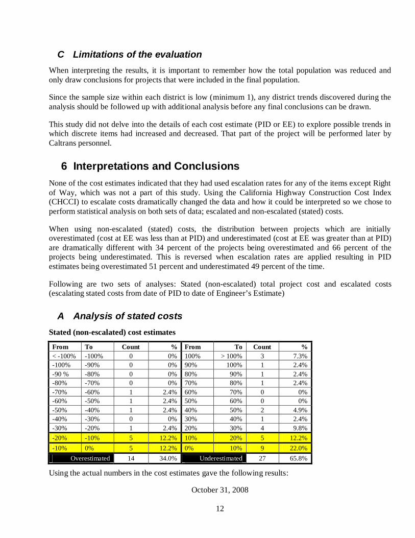
6 Interpretations and Conclusions None of the cost estimates indicated that they had used escalation rates for any of the items except Right of Way, which was not a part of this study. Using the California Highway Construction Cost Index (CHCCI) to escalate costs dramatically changed the data and how it could be interpreted so we chose to perform statistical analysis on both sets of data; escalated and non-escalated (stated) costs.
When using non-escalated (stated) costs, the distribution between projects which are initially overestimated (cost at EE was less than at PID) and underestimated (cost at EE was greater than at PID) are dramatically different with 34 percent of the projects being overestimated and 66 percent of the projects being underestimated. This is reversed when escalation rates are applied resulting in PID estimates being overestimated 51 percent and underestimated 49 percent of the time.
Following are two sets of analyses: Stated (non-escalated) total project cost and escalated costs (escalating stated costs from date of PID to date of Engineer’s Estimate)
A Analysis of stated costs Stated (non-escalated) cost estimates
From To Count % From To Count % < -100% -100% 0 0% 100% > 100% 3 7.3% -100% -90% 0 0% 90% 100% 1 2.4% -90 % -80% 0 0% 80% 90% 1 2.4% -80% -70% 0 0% 70% 80% 1 2.4% -70% -60% 1 2.4% 60% 70% 0 0% -60% -50% 1 2.4% 50% 60% 0 0% -50% -40% 1 2.4% 40% 50% 2 4.9% -40% -30% 0 0% 30% 40% 1 2.4% -30% -20% 1 2.4% 20% 30% 4 9.8% -20% -10% 5 12.2% 10% 20% 5 12.2% -10% 0% 5 12.2% 0% 10% 9 22.0%
Overestimated 14 34.0% Underestimated 27 65.8%
Using the actual numbers in the cost estimates gave the following results:
October 31, 2008
13
Comparison of PID and Engineer's Estimates(No Escalation)
0.0%
0.0%
0.0%
0.0%
2.4%
2.4%
2.4%
0.0%
2.4%
12.2
%
12.2
%
22.0
%
12.2
%
9.8%
2.4%
4.9%
0.0%
0.0%
2.4%
2.4%
2.4%
7.3%
0.0%
5.0%
10.0%
15.0%
20.0%
25.0%<-
100%
-100
% to
-90%
-90%
to -8
0%
-80%
to -7
0%
-70%
to -6
0%
-60%
to -5
0%
-50%
to -4
0%
-40%
to -3
0%
-30%
to -2
0%
-20%
to -1
0%
-10%
to 0
%
0% to
10%
10%
to 2
0%
20%
to 3
0%
30%
to 4
0%
40%
to 5
0%
50%
to 6
0%
60%
to 7
0%
70%
to 8
0%
80%
to 9
0%
90%
to 1
00%
>100
%
Percent Difference
Perc
ent o
f Pro
ject
s w
ithin
Ran
ge 9.8 % 58.5 % 31.7 %
How to read the graph:
This graph displays the gap between Project Initiation Document cost estimates and Engineer’s Estimates measured in percent ((EE-PID)/PID). Each bar represents the percentage of projects that fell within that 10 percent range.
Positive differences indicate that the cost estimate increased from PID to EE (was underestimated at PID), negative differences indicate that the cost estimate decreased (overestimated at PID).
Conclusion:
Fifty-nine percent of the projects (shown in the yellow box) are within the goal that the IDC/Caltrans Task Force had set (+/- 20%).
A majority (66 percent) of projects are underestimated in the Planning Phase, meaning that the cost estimate increased from PID to EE (positive numbers in the graph)
October 31, 2008
14
Stated (non-escalated) cost estimates – Other statistics
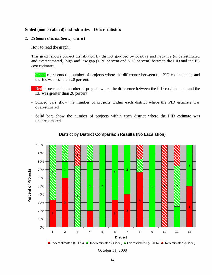
1. Estimate distribution by district
How to read the graph:
This graph shows project distribution by district grouped by positive and negative (underestimated and overestimated), high and low gap (> 20 percent and < 20 percent) between the PID and the EE cost estimates.
- Green represents the number of projects where the difference between the PID cost estimate and the EE was less than 20 percent.
- Red represents the number of projects where the difference between the PID cost estimate and the EE was greater than 20 percent
- Striped bars show the number of projects within each district where the PID estimate was overestimated.
- Solid bars show the number of projects within each district where the PID estimate was underestimated.
District by District Comparison Results (No Escalation)
1
3
1
12
4
1
1
3 2
23
1
1
1
2
1
3
1
1
2
11
1
1
0%
10%
20%
30%
40%
50%
60%
70%
80%
90%
100%
1 2 3 4 5 6 7 8 9 10 11 12
District
Perc
ent o
f Pro
ject
s
Underestimated (> 20%) Underestimated (< 20%) Overestimated (< 20%) Overestimated (> 20%)

October 31, 2008
15
Conclusion:
No significant trends are apparent. All estimates for Districts 5 and 9 fall within the goal of +/- 20 percent, but these districts have only two and one projects respectively. If any trends had been found, they would have required follow up with further analysis due to the small sample size within each district
2. Project distribution by PID cost range
How to read the graph:
This graph shows project distribution by cost range grouped by positive and negative (underestimated and overestimated), high and low gap (> 20 percent and < 20 percent) between the PID and the EE cost estimates.
- Green represents the number of projects where the difference between the PID cost estimate and the EE was less than 20 percent.
a. Red represents the number of projects where the difference between the PID cost estimate and the EE was greater than 20 percent
b. Striped bars show the number of projects within each district where the PID estimate was overestimated.
c. Solid bars show the number of projects within each district where the PID estimate was underestimated.
Conclusion:
Each cost range has nearly equal numbers in the high and low gap (> 20 percent and < 20 percent) except for projects in the $2 million to $5 million range where eleven out of eighteen projects are within the low gap category (less than 20%).
Further investigation could be performed, within the details of each estimate, to find out if this is a significant trend or merely a coincidence.

October 31, 2008
16
Cost Category Comparison Results (No Escalation)
55
1
7
2
54
1
1
2
32
21
0%
10%
20%
30%
40%
50%
60%
70%
80%
90%
100%
$1,000,000 to
$1,999,999
$2,000,000 to
$4,999,999
$5,000,000 to
$9,999,999
$10,000,000 to
$25,000,000
Cost Category
Perc
ent o
f Pro
ject
s
Underestimated (> 20%) Underestimated (< 20%) Overestimated (< 20%) Overestimated (> 20%)
3. Project distribution by PID Type
How to read the graph:
This graph shows project distribution by PID Type grouped by positive and negative (underestimated and overestimated), high and low gap (> 20 percent and < 20 percent) between the PID and the EE cost estimates. The x-axis shows the types of PID.
- Green represents the number of projects where the difference between the PID cost estimate and the EE was less than 20 percent.
a. Red represents the number of projects where the difference between the PID cost estimate and the EE was greater than 20 percent
b. Striped bars show the number of projects within each district where the PID estimate was overestimated.
c. Solid bars show the number of projects within each district where the PID estimate was underestimated.

October 31, 2008
17
PID Type Results (No Escalation)
1
5
1
14 4
31
24
2
1
44
121
0%
10%
20%
30%
40%
50%
60%
70%
80%
90%
100%
CAPM PR FPSR PPPR PR PSR PSR/PR PSSR
PID Type
Perc
ent o
f Pro
ject
s
Underestimated (> 20%) Underestimated (< 20%) Overestimated (< 20%) Overestimated (> 20%)
Conclusion:
No significant trend is discovered in this graph to indicate differences in results based on the PID Type.
4. Project distribution by Elapsed Time between PID and EE
How to read the graph:
This graph shows project distribution by time elapsed between the date of the PID estimate and the date of the Engineer’s Estimate. The results are grouped by positive and negative (underestimated and overestimated), high and low gap (> 20 percent and < 20 percent) between the PID and the EE cost estimates. The x-axis shows the types of PID.
- Green represents the number of projects where the difference between the PID cost estimate and the EE was less than 20 percent.
- Red represents the number of projects where the difference between the PID cost estimate and the EE was greater than 20 percent

October 31, 2008
18
- Striped bars show the number of projects within each district where the PID estimate was overestimated.
- Solid bars show the number of projects within each district where the PID estimate was underestimated.
Time Comparison Results (No Escalation)
3
3
5
3
2
3
4
3
3
2
2
2
2 2
1
1
0%
10%
20%
30%
40%
50%
60%
70%
80%
90%
100%
< 6 mos. 7 mos. to
12 mos.
13 mos. to
18 mos.
19 mos. to
24 mos.
25 mos.to
60 mos.
> 60 mos.
Time Between PID and Engineer's Estimates
Perc
ent o
f Pro
ject
s
Underestimated (> 20%) Underestimated (< 20%) Overestimated (< 20%) Overestimated (> 20%)
Conclusion:
This graph shows that two-thirds of the projects that are completed under 12 months (from PID estimate to Engineer’s Estimate) fall within the target of +/- 20 percent. A similar result is achieved for projects in the 25 to 60 month category.
B Analysis of escalated costs A secondary set of analyses was performed applying escalation rates to escalate the total amount of each cost from the PID date to the Engineer’s Estimate date. Four different escalation rates were tested to see which provided the best results: three percent annual escalation rate, California Highway Construction Cost Index, Engineering News Record Construction (ENR) Index, and the Global Insights (GI) Highway Construction Cost Index.

October 31, 2008
19
How to read the graphs:
The graphs below display the gap between the escalated Project Initiation Document cost estimates and Engineer’s Estimates measured in percent ((EE-PID)/PID). Each bar represents the percentage of projects that fell within that 10 percent range.
Positive differences indicate that the cost estimate increased from PID to EE (was underestimated at PID), negative differences indicate that the cost estimate decreased (overestimated at PID).
Bars within the yellow box indicate those projects that are within the goal that the IDC/Caltrans Task Force had set (+/- 20%).
Three Percent Annual Escalation:
The chart below shows the comparison of the PID estimate escalated at three percent per year to the Engineer’s Estimate. Three percent was chosen as one of the rates to be tested since this was historically used by Headquarters Programming to escalate projects costs until 2007. With the three percent escalation rate applied, slightly fewer projects fall within the +/- 20 percent target range than the non-escalated data (56.1 percent versus 58.5 percent). Slightly fewer projects are underestimated by greater than 20 percent (26.8 percent versus 31.7 percent).
Comparison of PID and Engineer's Estimates(Using a 3% Escalation Rate)
0.0%
0.0%
0.0%
0.0%
2.4%
4.9%
0.0%
2.4%
7.3%
14.6
%
19.5
%
14.6
%
7.3%
12.2
%
0.0%
0.0%
2.4%
4.9%
4.9%
2.4%
0.0%
0.0%
0.0%
5.0%
10.0%
15.0%
20.0%
25.0%
<-10
0%
-100
% to
-90%
-90%
to -8
0%
-80%
to -7
0%
-70%
to -6
0%
-60%
to -5
0%
-50%
to -4
0%
-40%
to -3
0%
-30%
to -2
0%
-20%
to -1
0%
-10%
to 0
%
0% to
10%
10%
to 2
0%
20%
to 3
0%
30%
to 4
0%
40%
to 5
0%
50%
to 6
0%
60%
to 7
0%
70%
to 8
0%
80%
to 9
0%
90%
to 1
00%
>100
%
Percent Difference
Perc
ent o
f Pro
ject
s w
ithin
Ran
ge 17.1 % 56.1 % 26.8 %

October 31, 2008
20
California Highway Construction Cost Index (CHCCI):
The California Highway Construction Cost Index is maintained by the Division of Engineering Services – Office of Office Engineer. It is based on the unit costs of seven common work items used on Caltrans projects and is used to show cost growth from a historical perspective. Using the CHCCI to escalate the PID costs causes a significant shift in the percent differences between the PID and Engineer’s Estimates. Fewer projects fall within the +/- 20 percent range than with the non-escalated data (48.8 percent versus 58.5 percent). Significantly fewer projects are underestimated by greater the 20 percent (4.9 percent versus 31.7 percent). Using the CHCCI causes 95.1 percent of the projects to fall below 120% of the PID estimate. At this time, Office Engineer does not perform any projections for the CHCCI for use in escalating projects into the future.
Comparison of PID and Engineer's Estimates(Using CHCCI Escalation Rates)
0.0%
0.0%
0.0%
2.4%
2.4%
4.9%
17.1
%
7.3%
12.2
%
12.2
%
12.2
%
14.6
%
9.8%
2.4%
2.4%
0.0%
0.0%
0.0%
0.0%
0.0%
0.0%
0.0%
0.0%
5.0%
10.0%
15.0%
20.0%
25.0%
<-10
0%
-100
% to
-90%
-90%
to -8
0%
-80%
to -7
0%
-70%
to -6
0%
-60%
to -5
0%
-50%
to -4
0%
-40%
to -3
0%
-30%
to -2
0%
-20%
to -1
0%
-10%
to 0
%
0% to
10%
10%
to 2
0%
20%
to 3
0%
30%
to 4
0%
40%
to 5
0%
50%
to 6
0%
60%
to 7
0%
70%
to 8
0%
80%
to 9
0%
90%
to 1
00%
>100
%Percent Difference
Perc
ent o
f Pro
ject
s w
ithin
Ran
ge
CHCCI - California Highway Construction Cost Index
46.3 % 48.8 % 4.9 %
Engineering News Record (ENR) Construction Cost Index:
Engineering News Record provides a Construction Cost Index based on a basket of goods including labor and materials. It is updated quarterly and is projected up to ten years into the future. Applying this index to the PID cost estimates results in fewer projects falling within the target range than the non-escalated estimates (53.7 percent versus 58.5 percent). Slightly fewer projects are underestimated by greater than 20 percent (24.4 percent versus 31.7 percent).
October 31, 2008
21
Comparison of PID and Engineer's Estimates(Using ENR Escalation Rates)
0.0%
0.0%
0.0%
0.0%
2.4%
4.9%
0.0%
2.4%
12.2
%
17.1
%
14.6
%
12.2
%
9.8%
9.8%
0.0%
0.0%
4.9%
2.4%
7.3%
0.0%
0.0%
0.0%
0.0%
5.0%
10.0%
15.0%
20.0%
25.0%<-
100%
-100
% to
-90%
-90%
to -8
0%
-80%
to -7
0%
-70%
to -6
0%
-60%
to -5
0%
-50%
to -4
0%
-40%
to -3
0%
-30%
to -2
0%
-20%
to -1
0%
-10%
to 0
%
0% to
10%
10%
to 2
0%
20%
to 3
0%
30%
to 4
0%
40%
to 5
0%
50%
to 6
0%
60%
to 7
0%
70%
to 8
0%
80%
to 9
0%
90%
to 1
00%
>100
%
Percent Difference
Perc
ent o
f Pro
ject
s w
ithin
Ran
ge
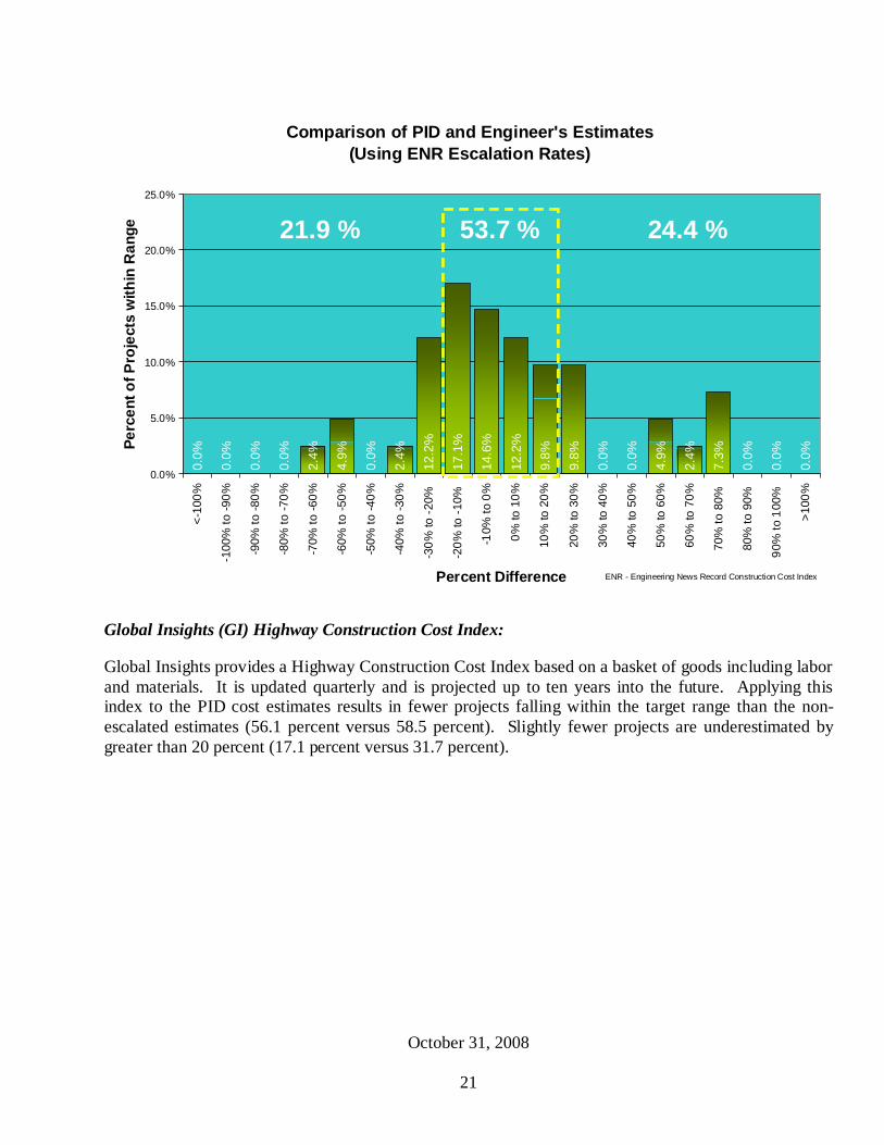
ENR - Engineering News Record Construction Cost Index
21.9 % 53.7 % 24.4 %
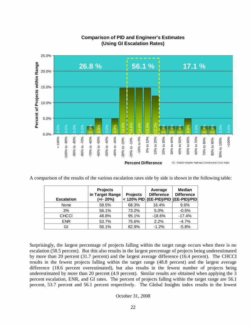
Global Insights (GI) Highway Construction Cost Index:
Global Insights provides a Highway Construction Cost Index based on a basket of goods including labor and materials. It is updated quarterly and is projected up to ten years into the future. Applying this index to the PID cost estimates results in fewer projects falling within the target range than the non-escalated estimates (56.1 percent versus 58.5 percent). Slightly fewer projects are underestimated by greater than 20 percent (17.1 percent versus 31.7 percent).
October 31, 2008
22
Comparison of PID and Engineer's Estimates(Using GI Escalation Rates)
0.0%
0.0%
0.0%
0.0%
2.4%
4.9%
0.0%
4.9%
14.6
%
14.6
%
14.6
%
14.6
%
12.2
%
2.4%
2.4%
2.4%
4.9%
0.0%
2.4%
2.4%
0.0%
0.0%
0.0%
5.0%
10.0%
15.0%
20.0%
25.0%<-
100%
-100
% to
-90%
-90%
to -8
0%
-80%
to -7
0%
-70%
to -6
0%
-60%
to -5
0%
-50%
to -4
0%
-40%
to -3
0%
-30%
to -2
0%
-20%
to -1
0%
-10%
to 0
%
0% to
10%
10%
to 2
0%
20%
to 3
0%
30%
to 4
0%
40%
to 5
0%
50%
to 6
0%
60%
to 7
0%
70%
to 8
0%
80%
to 9
0%
90%
to 1
00%
>100
%
Percent Difference
Perc
ent o
f Pro
ject
s w
ithin
Ran
ge
GI - Global Insights Highway Construction Cost Index
26.8 % 56.1 % 17.1 %
A comparison of the results of the various escalation rates side by side is shown in the following table:
Escalation
Projects in Target Range
(+/- 20%) Projects
< 120% PID
Average Difference
(EE-PID)/PID
Median Difference
(EE-PID)/PID None 58.5% 68.3% 16.4% 9.6% 3% 56.1% 73.2% 5.0% -0.5%
CHCCI 48.8% 95.1% -18.6% -17.4% ENR 53.7% 75.6% 2.2% -4.7% GI 56.1% 82.9% -1.2% -5.8%
Surprisingly, the largest percentage of projects falling within the target range occurs when there is no escalation (58.5 percent). But this also results in the largest percentage of projects being underestimated by more than 20 percent (31.7 percent) and the largest average difference (16.4 percent). The CHCCI results in the fewest projects falling within the target range (48.8 percent) and the largest average difference (18.6 percent overestimated), but also results in the fewest number of projects being underestimated by more than 20 percent (4.9 percent). Similar results are obtained when applying the 3 percent escalation, ENR, and GI rates. The percent of projects falling within the target range are 56.1 percent, 53.7 percent and 56.1 percent respectively. The Global Insights index results in the lowest

October 31, 2008
23
average difference between PID and EE (1.2 percent overestimated) and the second lowest percentage of projects being underestimated by more than 20 percent (17.1 percent). For the remainder of the analysis of escalated costs, the Global Insights results will be used.
Escalating the cost estimates using the Global Insights (GI) Highway Construction Cost Index gave the following results:
Escalated cost estimates
From To Count % From To Count % < -100% -100% 0 0% 100% > 100% 0 0.0%
-100% -90% 0 0% 90% 100% 0 0.0% -90 % -80% 0 0% 80% 90% 1 2.4% -80% -70% 0 0% 70% 80% 1 2.4% -70% -60% 1 2.4% 60% 70% 0 0% -60% -50% 2 4.9% 50% 60% 2 4.9% -50% -40% 0 0.0% 40% 50% 1 2.4% -40% -30% 2 4.9% 30% 40% 1 2.4% -30% -20% 6 14.6% 20% 30% 1 2.4% -20% -10% 6 14.6% 10% 20% 5 12.2% -10% 0% 6 14.6% 0% 10% 6 14.6% Overestimated 23 56.1% Underestimated 18 43.9%
Using the GI index results in 56.1 percent of the projects being overestimated at the PID stage and 43.9 percent of the projects being underestimated.
Escalated cost estimates – Other statistics
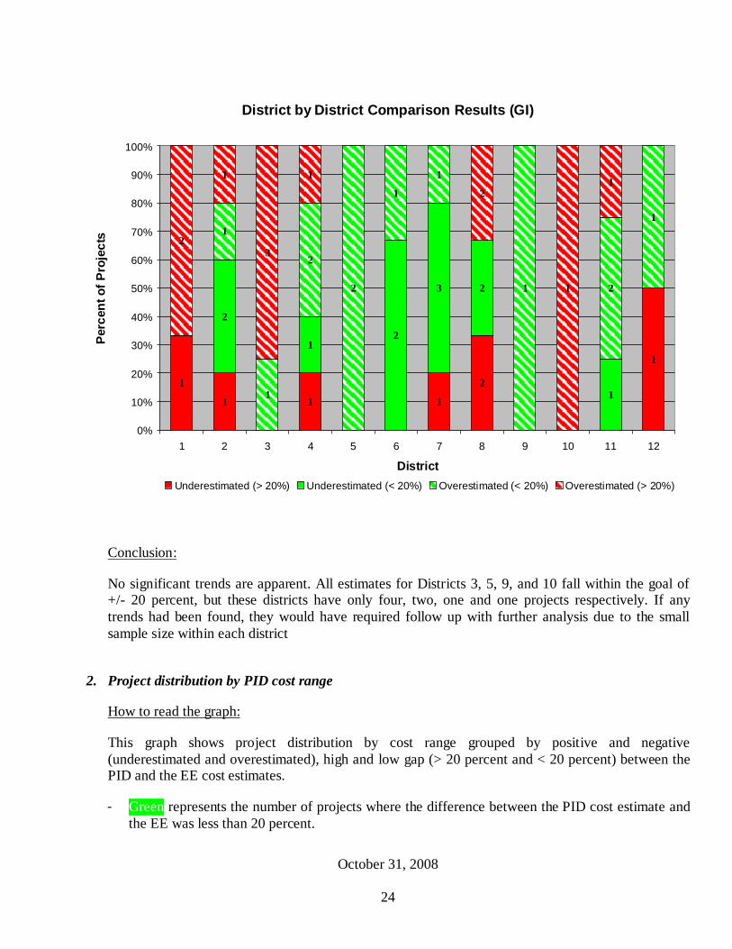
1. Estimate distribution by district
How to read the graph:
This graph shows project distribution by district grouped by positive and negative (underestimated and overestimated), high and low gap (> 20 percent and < 20 percent) between the PID and the EE cost estimates.
- Green represents the number of projects where the difference between the PID cost estimate and the EE was less than 20 percent.
- Red represents the number of projects where the difference between the PID cost estimate and the EE was greater than 20 percent
- Striped bars show the number of projects within each district where the PID estimate was overestimated.
- Solid bars show the number of projects within each district where the PID estimate was underestimated.
October 31, 2008
24
District by District Comparison Results (GI)
1
1 1 1
2
1
2
12
3
11
2
2
1
1
1 2
1
3
2
1
1
2
1
11
2
0%
10%
20%
30%
40%
50%
60%
70%
80%
90%
100%
1 2 3 4 5 6 7 8 9 10 11 12
District
Perc
ent o
f Pro
ject
s
Underestimated (> 20%) Underestimated (< 20%) Overestimated (< 20%) Overestimated (> 20%)
Conclusion:
No significant trends are apparent. All estimates for Districts 3, 5, 9, and 10 fall within the goal of +/- 20 percent, but these districts have only four, two, one and one projects respectively. If any trends had been found, they would have required follow up with further analysis due to the small sample size within each district
2. Project distribution by PID cost range
How to read the graph:
This graph shows project distribution by cost range grouped by positive and negative (underestimated and overestimated), high and low gap (> 20 percent and < 20 percent) between the PID and the EE cost estimates.
- Green represents the number of projects where the difference between the PID cost estimate and the EE was less than 20 percent.
October 31, 2008
25
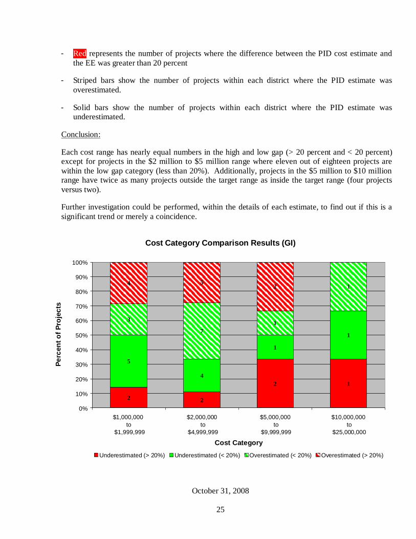
- Red represents the number of projects where the difference between the PID cost estimate and the EE was greater than 20 percent
- Striped bars show the number of projects within each district where the PID estimate was overestimated.
- Solid bars show the number of projects within each district where the PID estimate was underestimated.
Conclusion:
Each cost range has nearly equal numbers in the high and low gap (> 20 percent and < 20 percent) except for projects in the $2 million to $5 million range where eleven out of eighteen projects are within the low gap category (less than 20%). Additionally, projects in the $5 million to $10 million range have twice as many projects outside the target range as inside the target range (four projects versus two).
Further investigation could be performed, within the details of each estimate, to find out if this is a significant trend or merely a coincidence.
Cost Category Comparison Results (GI)
2 2
14
1
3
71
2
2
5
1
154
0%
10%
20%
30%
40%
50%
60%
70%
80%
90%
100%
$1,000,000 to
$1,999,999
$2,000,000 to
$4,999,999
$5,000,000 to
$9,999,999
$10,000,000 to
$25,000,000
Cost Category
Perc
ent o
f Pro
ject
s
Underestimated (> 20%) Underestimated (< 20%) Overestimated (< 20%) Overestimated (> 20%)

October 31, 2008
26
3. Project distribution by PID Type
How to read the graph:
This graph shows project distribution by PID Type grouped by positive and negative (underestimated and overestimated), high and low gap (> 20 percent and < 20 percent) between the PID and the EE cost estimates. The x-axis shows the types of PID.
- Green represents the number of projects where the difference between the PID cost estimate and the EE was less than 20 percent.
- Red represents the number of projects where the difference between the PID cost estimate and the EE was greater than 20 percent
- Striped bars show the number of projects within each district where the PID estimate was overestimated.
- Solid bars show the number of projects within each district where the PID estimate was underestimated.
PID Type Results (GI)
1
1
17 1
1 1
14
1
1
2
4
32
14
41
0%
10%
20%
30%
40%
50%
60%
70%
80%
90%
100%
CAPM PR FPSR PPPR PR PSR PSR/PR PSSR
PID Type
Perc
ent o
f Pro
ject
s
Underestimated (> 20%) Underestimated (< 20%) Overestimated (< 20%) Overestimated (> 20%)

October 31, 2008
27
Conclusion:
The only significant trend in this graph is that projects with a PSR/PR fall within the target range twice as often as fall outside this range (10 projects versus 5 projects). This is likely due to the fact that significantly more effort is applied to a PSR/PR document than to the other types.
4. Project distribution by Elapsed Time between PID and EE
How to read the graph:
This graph shows project distribution by time elapsed between the date of the PID estimate and the date of the Engineer’s Estimate. The results are grouped by positive and negative (underestimated and overestimated), high and low gap (> 20 percent and < 20 percent) between the PID and the EE cost estimates. The x-axis shows the types of PID.
- Green represents the number of projects where the difference between the PID cost estimate and the EE was less than 20 percent.
- Red represents the number of projects where the difference between the PID cost estimate and the EE was greater than 20 percent
- Striped bars show the number of projects within each district where the PID estimate was overestimated.
- Solid bars show the number of projects within each district where the PID estimate was underestimated.

October 31, 2008
28
Time Comparison Results (GI)
11
4
42
2
1
3
1
4
1
2
2
2 4
32
1
1
0%
10%
20%
30%
40%
50%
60%
70%
80%
90%
100%
< 6 mos. 7 mos. to
12 mos.
13 mos. to
18 mos.
19 mos. to
24 mos.
25 mos.to
60 mos.
> 60 mos.
Time Between PID and Engineer's Estimates
Perc
ent o
f Pro
ject
s
Underestimated (> 20%) Underestimated (< 20%) Overestimated (< 20%) Overestimated (> 20%)
Conclusion:
This graph shows that 75 percent of the projects that are completed within 12 months (from PID estimate to Engineer’s Estimate) fall within the target of +/- 20 percent. A similar result is achieved for projects in the 19 to 24 month category.
7 Recommendations Caltrans has already decided to implement the first and most important recommendation as a result of this project, which is to perform a detailed analysis of the PID and Engineer’s Estimates to look for trends within discrete work items and categories of work items.
Other Recommendations:
Define acceptable range
This project provided analysis of the gap between planning level cost estimates and Engineer’s Estimate and showed that 58.5 percent of stated (non-escalated) PID Cost Estimates are within the acceptable range (+/- 20 percent) of the subsequent Engineer’s Estimate (56.1 percent using escalated PID Cost estimates).

October 31, 2008
29
There was however, no set expectation or benchmarks identified prior to this study as to what percent of projects falling within the desired range was acceptable. It is unreasonable to expect that all projects could fall within this range with even the most sophisticated cost estimating system in place. It is recommended that these findings be compared to results from other states to decide whether this is an acceptable proportion.
Transparent Cost Management – Ability to monitor costs
The Department’s goal for managing costs is to be able to identify potential problems while they can still be managed. This is difficult, if not impossible in the current process where the cost estimate details are not easily accessible to anyone outside the Project Development Team. Also, it seems that in most districts the planning level cost estimates are available in paper-based copies only, which does not support an on-going efficient trend analysis.
When the Engineer’s Estimates are entered into BEES, there is more transparency, but since both estimates do not reside in the same system it does not allow for the type of analysis that was performed in this project.
Define Standards and Format
With directives as detailed as the PDPM Chapter 20 and appendix AA it is hard to believe that there would be any problems in reviewing cost estimates from different projects. There did, however, turn out to be more differences in format than expected. Here are some of the areas that were found to be inconsistent:
- Items included The PDPM shows work divided into 8 sections but many of the estimates had other sections included, the same sections but listed differently, or the same sections with different items of work identified within them.
- Contingency
o Between 5 and 25% (Average 20%) o Calculated on sum of items contained in various categories (e.g. 1-5 or 1-6)
- Format Most districts seem to be using formats similar to the one indicated in the PDPM except for District 11 which uses a far more detailed format.
For the sake of future analysis and similar projects it is recommended that the Department implement a system which encourages the same format to be used in all districts/regions.
Update the Archive/Storage System
The majority of time spent on this project was during the document gathering process. The current archiving routines are time consuming and inefficient. Project documents are created in hard copies (paper) form and each district stores original project documents locally and forwards copies to

October 31, 2008
30
headquarters in Sacramento. The problem seems to be that some districts are not as punctual in forwarding copies to Headquarters.
However, even if all the districts submitted copies of their project documents promptly, the headquarters archive is close to capacity leading to an overflow of project documents being stored in several alternative storage areas. This makes the document retrieval process lengthy and inefficient.
The recommendation is for the Department to transition from a hard to a soft copy archive solution.
From Paper-Based to Electronic System
If the Department decides to implement an electronic statewide system for recording cost estimates, they would realize all but one of the recommendations above
- Increase the transparency and add the ability to monitor and manage costs on an ongoing basis.
- Standards and formats could be hard-coded into the system forcing discrete items to be put in comparable categories or followed by explanations where exceptions are needed.
- Provide headquarters live updated cost estimates without the need for more storage space or document managers/personnel.
Escalation rates
To escalate PID cost estimates from current year costs we analyzed various escalation rates. The Department could, as a next step, look at other types of escalation rates either construction specific or the generic consumer price index of the same years to see if they produce similar trends.
Appendices 1. IDC – Caltrans Committee Task Force No. 2 Final Report
2. Data Tables and Charts No Escalation 3 percent Escalation CHCCI Escalation ENR Escalation GI Escalation
3. District by District Comparison Charts No Escalation 3 percent Escalation GI Escalation
4. Cost Category Comparison Charts No Escalation 3 percent Escalation GI Escalation
5. PID Type Comparison Charts No Escalation 3 percent Escalation GI Escalation
6. Elapsed Time Comparison Charts No Escalation 3 percent Escalation GI Escalation

Appendix 1
IDC – Caltrans Committee Task Force No. 2 Final Report

July 9, 2007
IDC – Caltrans Committee Task Force No. 2
Improve Capital Cost Estimating – Final Report
Introduction: This task force was developed to improve the accuracy and level of confidence in project capital cost estimates. The members met on a monthly basis between May 2006 and March 2007 to identify needed actions and to report back to the team on completed action items. The task force developed the following expected results:
1. Planning level cost estimates are within 20 percent of subsequent engineers estimates. 2. Engineers estimates at advertisement are within 10 percent of the low bid 3. The final cost is within 5 percent of the awarded amount.
Scope of Activities: The task force members identified some key activities to improve the quality of project capital costs. The following is the scope of activities developed:
1. Collect baseline data on current cost estimating accuracy. 2. Establish performance measures and benchmarks for comparison. 3. Review existing cost estimating practices, procedures, and tools. 4. Identify potential new cost estimating tools for development or use. 5. Define roles and responsibilities for providing quality cost estimates. 6. Develop Quality Control, Quality Assurance, and Independent Assurance processes,
policies, and guidelines for cost estimating. 7. Develop training in order to implement improvements. 8. Monitor and report on performance measures. 9. Incorporate lessons learned for continuous improvement.
The task force made an attempt to address each of these activities. Some activities have been completed, some are ongoing, and others have not been completed for various reasons. The following section lists the activities and their status. Status of Activities: Collect Baseline Data on Current Cost Estimating Accuracy
The task force has been collecting and monitoring baseline data to measure cost estimating accuracy. Caltrans Office Engineer produces a quarterly report comparing bid results to the Engineer’s Estimate. Office Engineer also produced a report showing this same data for previous years. This information is now reported to Caltrans management on a regular basis. Other baseline data has proven to be more elusive as Caltrans does not have a central database to collect this data. In particular, the comparison between
July 9, 2007
planning level estimates compared to Engineer’s Estimate is not tracked. The cost growth during construction is tracked by Construction and is being reported to management.
Establish performance measures and benchmarks for comparison
As noted earlier, performance measures have been developed and are being monitored. The task force attempted to identify benchmarks with the consulting industry and other public agencies. Data was not readily available due to confidentiality concerns or because the data was not collected and tracked in a way that could be shared. Division of Design performed a survey of other State Departments of Transportation (DOTs) to see how other public agencies were performing in regards to engineer’s estimates versus low bids. Data was provided by ten State DOTs. Most states had more than 45 percent of their low bids within +/- 10 percent of their engineer’s estimates in fiscal year 2006. The Department has only 33.5 percent fall within this range during the same period.
Review existing cost estimating practices, procedures, and tools.
The Department has completed a review of its current practices and procedures. The cost estimating practices and procedures are well defined and thorough. Existing tools available are estimate formats and bid history data. Chapter 20 has been revised to incorporate many of the new policies that have occurred recently.
Identify potential new cost estimating tools for development or use.
The Department has subscribed to a (Global Insights) to provide data needed to develop market based cost escalation. AASHTOWare or other cost estimating software tools are being evaluated to assist the Department in developing and documenting cost-estimates. These cost-estimating tools will provide flexibility in developing construction-based estimates or parametric estimates in addition to the historic bid-based estimates. One of the new tools that the Department has undertaken is Cost Risk Studies on projects. The Department has performed a pilot, which included five projects to date. The intent of this tool is to review the projects and identify risk elements that could impact the project cost. Each risk element is assigned a range of costs and a risk contingency is determined via a Monte Carlo simulation. The Department intends to evaluate the success of this pilot and decide whether to pursue this tool on a wider range of projects.
Define roles and responsibilities for providing quality cost estimates.
The Project Development Procedures Manual clearly defines the roles and responsibilities for providing quality cost estimates. New policy has been implemented requiring District Directors to certify the cost estimates for projects greater than $5 million.
July 9, 2007
The Department is currently evaluating the feasibility of adding a Cost Estimator classification. A study is currently underway by personnel. Transportation engineers, who develop a few estimates per year, prepare most estimates currently. The goal of the Cost Estimator classification would be to retain expertise in a cost estimating unit. If the Department is able to utilize the Department of General Services Cost Estimator classification, results could be available in about six months. Otherwise, this study could take a period of years.
Develop Quality Control, Quality Assurance, and Independent Assurance processes, policies, and guidelines for cost estimating.
Each District was required to develop a Quality Control/Quality Assurance plan for project cost estimates. These have now been collected, published in a report, and shared statewide. The Division of Engineering Services has initiated contracts to perform independent estimates on all projects greater than $5 million. These independent estimates will provide the basis of an Independent Assurance process.
Develop training in order to implement improvements.
With the assistance of the task force, the Department has identified several training opportunities and is currently providing this training to its employees. This will continue over the next couple of years. The goal is to provide training for 80 employees this fiscal year.
Monitor and report on performance measures.
As noted previously, the performance measures are being monitored and reported to management regularly. The Department will continue to develop methods to capture the planning measures, which are not currently available.
Incorporate lessons learned for continuous improvement.
The Department will continue to identify best practices and implement changes to its policy and procedures as lessons are learned. One of the ways the Department is sharing this information currently is through its development of a Cost-Estimating webpage. This page has links to policy and procedure documents as well as links to other information of importance to the Departments cost estimators.
Conclusion Cost-estimating is an evolving practice and market conditions are constantly changing. Of primary importance is to put practices and tools in place to react to these changes. The Task Force has developed a baseline for performance and has identified areas of improvement. The Department is now in a position to implement many of these items. The Department will also continue to monitor and make continuous improvements to ensure that its cost estimating

July 9, 2007
processes are working. The Task Force members have agreed to act as an ad hoc group when and if cost estimating issues arise. Their primary purpose has been fulfilled.

Appendix 2
Data Tables and Charts No Escalation
3 percent Escalation CHCCI Escalation
ENR Escalation GI Escalation

No Escalation Data Table
District EA Type of PID PID Estimate
PID Estimate
Date
Time Elapsed
(mos) Engineer's Estimate Cost Category EE DateType of EE
% Difference (no escalation)
% Difference (w escalation)
01 292004 PSR $7,051,000 7/24/2001 70 $5,681,000 C 6/7/2007 F Final -19.4% #DIV/0!01 411804 PSR $1,270,000 8/25/2003 44 $2,291,000 B 5/2/2007 F 80.4% #DIV/0!01 422904 PR/PSR $1,310,000 1/3/2005 18 $1,152,000 A 6/29/2006 P (Prel -12.1% #DIV/0!02 359904 PSSR $4,206,000 9/1/2001 69 $8,954,000 C 6/4/2007 F 112.9% #DIV/0!02 374604 PSR $1,600,000 9/14/2001 56 $1,462,000 A 5/19/2006 P -8.6% #DIV/0!02 0C6804 PR/PSR $1,200,000 1/1/2004 37 $1,707,000 A 1/25/2007 F 42.3% #DIV/0!02 1C2304 PR/PSR $2,496,300 6/14/2004 23 $2,740,000 B 5/15/2006 P 9.8% #DIV/0!02 2C6504 PR/PSR $1,057,604 8/9/2005 20 $1,274,000 A 4/3/2007 P 20.5% #DIV/0!03 290904 PSSR $2,500,000 10/10/2001 62 $2,394,900 B 12/19/2006 P -4.2% #DIV/0!03 401804 PSR $2,151,000 3/18/2002 45 $2,004,000 B 12/14/2005 P -6.8% #DIV/0!03 2E1304 PSR $5,381,000 10/13/2005 11 $4,812,000 B 9/6/2006 P -10.6% #DIV/0!03 2E1504 PSR/PR $5,041,000 2/1/2006 3 $2,182,000 B 4/18/2006 P -56.7% #DIV/0!04 246804 HA28 $2,087,686 8/7/1997 110 $2,430,000 B 9/27/2006 P 16.4% #DIV/0!04 449404 PSSR $16,909,657 10/31/2001 39 $19,530,010 D 1/31/2005 P 15.5% #DIV/0!04 0A1304 PSR $2,922,000 1/1/2002 54 $3,319,000 B 6/21/2006 F 13.6% #DIV/0!04 0C7904 CAPM PR $4,722,000 8/27/1999 91 $9,356,000 C 4/10/2007 F 98.1% #DIV/0!04 3A3604 PSR/PR $1,755,600 1/13/2006 8 $1,409,000 A 9/1/2006 P -19.7% #DIV/0!05 0C5404 PSR $4,158,200 8/28/2000 63 $4,478,000 B 11/14/2005 P 7.7% #DIV/0!05 0N0904 PSSR $1,675,200 2/21/2006 9 $1,793,000 A 12/5/2006 F 7.0% #DIV/0!06 451604 PSR $2,450,000 1/1/2001 61 $2,737,000 B 2/6/2006 P 11.7% #DIV/0!06 0A3804 PR/PSR $1,476,100 5/27/2004 23 $1,925,000 A 4/12/2006 P 30.4% #DIV/0!06 0A8704 PSR $1,098,528 6/10/2005 10 $1,174,003 A 4/14/2006 P 6.9% #DIV/0!07 184904 CAPM PR $1,882,000 7/13/1999 84 $2,805,000 B 7/5/2006 P 49.0% #DIV/0!07 188804 PSR $896,600 11/24/1999 81 $1,935,000 A 8/10/2006 P 115.8% #DIV/0!07 210804 FPSR $3,002,000 9/8/2000 75 $3,290,000 B 12/11/2006 P 9.6% #DIV/0!07 257304 SPR/PSR $8,927,000 8/16/2006 0 $9,004,000 C 8/23/2006 P 0.9% #DIV/0!07 257704 PR/PSR $1,598,000 12/27/2005 11 $1,910,000 A 12/5/2006 P 19.5% #DIV/0!08 384204 PIP $6,739,140 4/26/2005 20 $11,837,000 D 12/21/2006 P 75.6% #DIV/0!08 476104 PSR $14,409,000 11/7/2000 65 $7,771,000 C 4/10/2006 P -46.1% #DIV/0!08 0F0204 PR/PSR $2,100,891 7/25/2005 10 $2,667,000 B 6/2/2006 P 26.9% #DIV/0!08 0F1404 PR/PSR $1,042,731 6/25/2005 9 $1,323,000 A 3/23/2006 P 26.9% #DIV/0!08 0G4604 PR $1,700,000 3/8/2006 8 $2,081,000 B 11/1/2006 P 22.4% #DIV/0!08 0G7204 CAPM PR $2,684,500 9/1/2005 18 $2,320,000 B 3/8/2007 F -13.6% #DIV/0!09 333004 CAPM PR $6,557,700 8/30/2005 21 $6,753,000 C 5/21/2007 F 3.0% #DIV/0!10 0N0204 PPPR $8,641,000 11/15/2005 18 $3,333,000 B 5/2/2007 F -61.4% #DIV/0!11 267404 PR/PSR $1,496,155 9/30/2005 15 $1,426,000 A 12/28/2006 P -4.7% #DIV/0!11 271204 PR/PSR $2,391,579 11/30/2005 15 $1,778,000 A 2/23/2007 F -25.7% #DIV/0!11 279804 PR/PSR $2,635,700 6/29/2006 5 $2,900,000 B 12/8/2006 F 10.0% #DIV/0!11 280104 PR/PSR $1,876,400 6/14/2006 8 $1,722,000 A 2/14/2007 F -8.2% #DIV/0!12 079304 PSR $1,882,000 8/14/1997 110 $4,441,000 B 10/3/2006 P 136.0% #DIV/0!12 0G4004 CAPM PR $15,735,000 4/1/2004 34 $16,207,000 D 2/2/2007 F 3.0% #DIV/0!
Average 16.4%Median 9.6%Std Deviation 43.5%Skew 103.3%Kutosis 125.0%

No Escalation Chart
Page 1
Comparison of PID and Engineer's Estimates(No Escalation)
0.0%
0.0%
0.0%
0.0%
2.4%
2.4%
2.4%
0.0%
2.4%
12.2
%
12.2
%
22.0
%
12.2
%
9.8%
2.4%
4.9%
0.0%
0.0%
2.4%
2.4%
2.4%
7.3%
0.0%
5.0%
10.0%
15.0%
20.0%
25.0%<-
100%
-100
% to
-90%
-90%
to -8
0%
-80%
to -7
0%
-70%
to -6
0%
-60%
to -5
0%
-50%
to -4
0%
-40%
to -3
0%
-30%
to -2
0%
-20%
to -1
0%
-10%
to 0
%
0% to
10%
10%
to 2
0%
20%
to 3
0%
30%
to 4
0%
40%
to 5
0%
50%
to 6
0%
60%
to 7
0%
70%
to 8
0%
80%
to 9
0%
90%
to 1
00%
>100
%
Percent Difference
Perc
ent o
f Pro
ject
s w
ithin
Ran
ge 9.8 % 58.5 % 31.7 %

3 Percent Escalation Data Table
District EA PID Estimate
PID Estimate
Date
Time Elapsed
(mos)Escalation
Factor Escalated PID Estimate Engineer's Estimate Cost Category EE Date% Difference
(no escalation)% Difference
(w escalation)01 292004 $7,051,000 7/24/2001 70 1.189 $8,386,835 $5,681,000 C 6/7/2007 -19.4% -32.3%01 411804 $1,270,000 8/25/2003 44 1.115 $1,416,195 $2,291,000 B 5/2/2007 80.4% 61.8%01 422904 $1,310,000 1/3/2005 18 1.045 $1,368,940 $1,152,000 A 6/29/2006 -12.1% -15.8%02 359904 $4,206,000 9/1/2001 69 1.186 $4,986,436 $8,954,000 C 6/4/2007 112.9% 79.6%02 374604 $1,600,000 9/14/2001 56 1.148 $1,837,407 $1,462,000 A 5/19/2006 -8.6% -20.4%02 0C6804 $1,200,000 1/1/2004 37 1.095 $1,313,859 $1,707,000 A 1/25/2007 42.3% 29.9%02 1C2304 $2,496,300 6/14/2004 23 1.058 $2,642,026 $2,740,000 B 5/15/2006 9.8% 3.7%02 2C6504 $1,057,604 8/9/2005 20 1.050 $1,110,464 $1,274,000 A 4/3/2007 20.5% 14.7%03 290904 $2,500,000 10/10/2001 62 1.166 $2,914,651 $2,394,900 B 12/19/2006 -4.2% -17.8%03 411804 $2,151,000 3/18/2002 45 1.117 $2,402,356 $2,004,000 B 12/14/2005 -6.8% -16.6%03 2E1304 $5,381,000 10/13/2005 11 1.027 $5,525,618 $4,812,000 B 9/6/2006 -10.6% -12.9%03 2E1504 $5,041,000 2/1/2006 3 1.006 $5,072,972 $2,182,000 B 4/18/2006 -56.7% -57.0%04 246804 $2,087,686 8/7/1997 110 1.310 $2,735,163 $2,430,000 B 9/27/2006 16.4% -11.2%04 449404 $16,909,657 10/31/2001 39 1.101 $18,614,689 $19,530,010 D 1/31/2005 15.5% 4.9%04 0A1304 $2,922,000 1/1/2002 54 1.141 $3,334,964 $3,319,000 B 6/21/2006 13.6% -0.5%04 0C7904 $4,722,000 8/27/1999 91 1.253 $5,914,779 $9,356,000 C 4/10/2007 98.1% 58.2%04 3A3604 $1,755,600 1/13/2006 8 1.019 $1,788,775 $1,409,000 A 9/1/2006 -19.7% -21.2%05 0C5404 $4,158,200 8/28/2000 63 1.167 $4,850,668 $4,478,000 B 11/14/2005 7.7% -7.7%05 0N0904 $1,675,200 2/21/2006 9 1.024 $1,714,722 $1,793,000 A 12/5/2006 7.0% 4.6%06 451604 $2,450,000 1/1/2001 61 1.163 $2,848,395 $2,737,000 B 2/6/2006 11.7% -3.9%06 0A3804 $1,476,100 5/27/2004 23 1.057 $1,560,219 $1,925,000 A 4/12/2006 30.4% 23.4%06 0A8704 $1,098,528 6/10/2005 10 1.025 $1,126,293 $1,174,003 A 4/14/2006 6.9% 4.2%07 184904 $1,882,000 7/13/1999 96 1.266 $2,382,496 $2,805,000 B 7/5/2007 49.0% 17.7%07 188804 $896,600 11/24/1999 81 1.219 $1,093,329 $1,935,000 A 8/10/2006 115.8% 77.0%07 210804 $3,002,000 9/8/2000 75 1.203 $3,612,021 $3,290,000 B 12/11/2006 9.6% -8.9%07 257304 $8,927,000 8/16/2006 0 1.001 $8,932,132 $9,004,000 C 8/23/2006 0.9% 0.8%07 257704 $1,598,000 12/27/2005 11 1.028 $1,642,970 $1,910,000 A 12/5/2006 19.5% 16.3%08 384204 $6,739,140 4/26/2005 20 1.050 $7,076,550 $11,837,000 D 12/21/2006 75.6% 67.3%08 476104 $14,409,000 11/7/2000 65 1.174 $16,915,147 $7,771,000 C 4/10/2006 -46.1% -54.1%08 0F0204 $2,100,891 7/25/2005 10 1.026 $2,154,521 $2,667,000 B 6/2/2006 26.9% 23.8%08 0F1404 $1,042,731 6/25/2005 9 1.022 $1,065,930 $1,323,000 A 3/23/2006 26.9% 24.1%08 0G4604 $1,700,000 3/8/2006 8 1.019 $1,732,836 $2,081,000 B 11/1/2006 22.4% 20.1%08 0G7204 $2,684,500 9/1/2005 18 1.046 $2,807,817 $2,320,000 B 3/8/2007 -13.6% -17.4%09 333004 $6,557,700 8/30/2005 21 1.052 $6,900,741 $6,753,000 C 5/21/2007 3.0% -2.1%10 0N0204 $8,641,000 11/15/2005 18 1.044 $9,023,110 $3,333,000 B 5/2/2007 -61.4% -63.1%11 267404 $1,496,155 9/30/2005 15 1.037 $1,552,215 $1,426,000 A 12/28/2006 -4.7% -8.1%11 271204 $2,391,579 11/30/2005 15 1.037 $2,480,171 $1,778,000 A 2/23/2007 -25.7% -28.3%11 279804 $2,635,700 6/29/2006 5 1.013 $2,670,335 $2,900,000 B 12/8/2006 10.0% 8.6%11 280104 $1,876,400 6/14/2006 8 1.020 $1,913,743 $1,722,000 A 2/14/2007 -8.2% -10.0%12 079304 $1,882,000 8/14/1997 110 1.310 $2,465,483 $4,441,000 B 10/3/2006 136.0% 80.1%12 0G4004 $15,735,000 4/1/2004 34 1.087 $17,110,967 $16,207,000 D 2/2/2007 3.0% -5.3%
Average 5.0%Median -0.5%Std Deviation 34.6%Skew 55.6%Kurtosis 34.9%
Comparison of PID and Engineer's Estimates(Using a 3% Escalation Rate)
0.0%
0.0%
0.0%
0.0%
2.4%
4.9%
0.0%
2.4%
7.3%
14.6
%
19.5
%
14.6
%
7.3%
12.2
%
0.0%
0.0%
2.4%
4.9%
4.9%
2.4%
0.0%
0.0%
0.0%
5.0%
10.0%
15.0%
20.0%
25.0%<-
100%
-100
% to
-90%
-90%
to -8
0%
-80%
to -7
0%
-70%
to -6
0%
-60%
to -5
0%
-50%
to -4
0%
-40%
to -3
0%
-30%
to -2
0%
-20%
to -1
0%
-10%
to 0
%
0% to
10%
10%
to 2
0%
20%
to 3
0%
30%
to 4
0%
40%
to 5
0%
50%
to 6
0%
60%
to 7
0%
70%
to 8
0%
80%
to 9
0%
90%
to 1
00%
>100
%
Percent Difference
Perc
ent o
f Pro
ject
s w
ithin
Ran
ge 17.1 % 56.1 % 26.8 %

California Highway Construction Cost Index Data Table
District EA PID Estimate
PID Estimate
Date
Time Elapsed
(mos)Begin
Index YearBegin Index
End Index Year End Index
Escalation Factor
Escalated PID Estimate Engineer's Estimate EE Date
% Difference (no escalation)
% Difference (w escalation)
01 292004 $7,051,000 7/24/2001 70 2000/01 150.150 2006/07 270.850 1.804 $12,719,037 $5,681,000 6/7/2007 -19.4% -55.3%01 411804 $1,270,000 8/25/2003 44 2002/03 145.400 2006/07 270.850 1.863 $2,365,746 $2,291,000 5/2/2007 80.4% -3.2%01 422904 $1,310,000 1/3/2005 18 2004 216.200 2005/06 274.450 1.269 $1,662,949 $1,152,000 6/29/2006 -12.1% -30.7%02 359904 $4,206,000 9/1/2001 69 2001 154.100 2006/07 270.850 1.758 $7,392,570 $8,954,000 6/4/2007 112.9% 21.1%02 374604 $1,600,000 9/14/2001 56 2001 154.100 2005/06 274.450 1.781 $2,849,578 $1,462,000 5/19/2006 -8.6% -48.7%02 0C6804 $1,200,000 1/1/2004 37 2003 148.600 2006 280.600 1.888 $2,265,949 $1,707,000 1/25/2007 42.3% -24.7%02 1C2304 $2,496,300 6/14/2004 23 2003/04 182.400 2005/06 274.450 1.505 $3,756,083 $2,740,000 5/15/2006 9.8% -27.1%02 2C6504 $1,057,604 8/9/2005 20 2004/05 242.250 2006 280.600 1.158 $1,225,031 $1,274,000 4/3/2007 20.5% 4.0%03 290904 $2,500,000 10/10/2001 62 2001 154.100 2006 280.600 1.821 $4,552,239 $2,394,900 12/19/2006 -4.2% -47.4%03 411804 $2,151,000 3/18/2002 45 2001 154.100 2005 268.300 1.741 $3,745,057 $2,004,000 12/14/2005 -6.8% -46.5%03 2E1304 $5,381,000 10/13/2005 11 2005 268.300 2006 280.600 1.046 $5,627,688 $4,812,000 9/6/2006 -10.6% -14.5%03 2E1504 $5,041,000 2/1/2006 3 2005 268.300 2005 268.300 1.000 $5,041,000 $2,182,000 4/18/2006 -56.7% -56.7%04 246804 $2,087,686 8/7/1997 110 1996/97 122.000 2006 280.600 2.300 $4,801,678 $2,430,000 9/27/2006 16.4% -49.4%04 449404 $16,909,657 10/31/2001 39 2001 154.100 2004 216.200 1.403 $23,723,996 $19,530,010 1/31/2005 15.5% -17.7%04 0A1304 $2,922,000 1/1/2002 54 2001 154.100 2005/06 274.450 1.781 $5,204,042 $3,319,000 6/21/2006 13.6% -36.2%04 0C7904 $4,722,000 8/27/1999 91 1998/99 133.900 2006 280.600 2.096 $9,895,394 $9,356,000 4/10/2007 98.1% -5.5%04 3A3604 $1,755,600 1/13/2006 8 2005 268.300 2006 280.600 1.046 $1,836,084 $1,409,000 9/1/2006 -19.7% -23.3%05 0C5404 $4,158,200 8/28/2000 63 1999/00 142.700 2005 268.300 1.880 $7,818,115 $4,478,000 11/14/2005 7.7% -42.7%05 0N0904 $1,675,200 2/21/2006 9 2005 268.300 2006 280.600 1.046 $1,751,998 $1,793,000 12/5/2006 7.0% 2.3%06 451604 $2,450,000 1/1/2001 61 2000 146.200 2005 268.300 1.835 $4,496,135 $2,737,000 2/6/2006 11.7% -39.1%06 0A3804 $1,476,100 5/27/2004 23 2003/04 182.400 2005 268.300 1.471 $2,171,259 $1,925,000 4/12/2006 30.4% -11.3%06 0A8704 $1,098,528 6/10/2005 10 2004/05 242.250 2005 268.300 1.108 $1,216,657 $1,174,003 4/14/2006 6.9% -3.5%07 184904 $1,882,000 7/13/1999 96 1998/99 133.900 2006/07 270.850 2.023 $3,806,869 $2,805,000 7/5/2007 49.0% -26.3%07 188804 $896,600 11/24/1999 81 1999 139.200 2005/06 274.450 1.972 $1,767,758 $1,935,000 8/10/2006 115.8% 9.5%07 210804 $3,002,000 9/8/2000 75 2000 146.200 2006 280.600 1.919 $5,761,705 $3,290,000 12/11/2006 9.6% -42.9%07 257304 $8,927,000 8/16/2006 0 2005/06 274.450 2005/06 274.450 1.000 $8,927,000 $9,004,000 8/23/2006 0.9% 0.9%07 257704 $1,598,000 12/27/2005 11 2005 268.300 2006 280.600 1.046 $1,671,259 $1,910,000 12/5/2006 19.5% 14.3%08 384204 $6,739,140 4/26/2005 20 2004 216.200 2006 280.600 1.298 $8,746,543 $11,837,000 12/21/2006 75.6% 35.3%08 476104 $14,409,000 11/7/2000 65 2000 146.200 2005 268.300 1.835 $26,442,782 $7,771,000 4/10/2006 -46.1% -70.6%08 0F0204 $2,100,891 7/25/2005 10 2004/05 242.250 2005/06 274.450 1.133 $2,380,143 $2,667,000 6/2/2006 26.9% 12.1%08 0F1404 $1,042,731 6/25/2005 9 2004/05 242.250 2005 268.300 1.108 $1,154,860 $1,323,000 3/23/2006 26.9% 14.6%08 0G4604 $1,700,000 3/8/2006 8 2005 268.300 2006 280.600 1.046 $1,777,935 $2,081,000 11/1/2006 22.4% 17.0%08 0G7204 $2,684,500 9/1/2005 18 2005 268.300 2006 280.600 1.046 $2,807,569 $2,320,000 3/8/2007 -13.6% -17.4%09 333004 $6,557,700 8/30/2005 21 2004/05 242.250 2006/07 270.850 1.118 $7,331,901 $6,753,000 5/21/2007 3.0% -7.9%10 0N0204 $8,641,000 11/15/2005 18 2005 268.300 2006/07 270.850 1.010 $8,723,127 $3,333,000 5/2/2007 -61.4% -61.8%11 267404 $1,496,155 9/30/2005 15 2005 268.300 2006 280.600 1.046 $1,564,745 $1,426,000 12/28/2006 -4.7% -8.9%11 271204 $2,391,579 11/30/2005 15 2005 268.300 2006 280.600 1.046 $2,501,219 $1,778,000 2/23/2007 -25.7% -28.9%11 279804 $2,635,700 6/29/2006 5 2005/06 274.450 2006 280.600 1.022 $2,694,762 $2,900,000 12/8/2006 10.0% 7.6%11 280104 $1,876,400 6/14/2006 8 2005/06 274.450 2006 280.600 1.022 $1,918,447 $1,722,000 2/14/2007 -8.2% -10.2%12 079304 $1,882,000 8/14/1997 110 1996/97 122.000 2006 280.600 2.300 $4,328,600 $4,441,000 10/3/2006 136.0% 2.6%12 0G4004 $15,735,000 4/1/2004 34 2003 148.600 2006 280.600 1.888 $29,712,254 $16,207,000 2/2/2007 3.0% -45.5%
Average -18.6%Median -17.4%Std Deviation 26.0%Skew -5.8%Kurtosis -87.4%

Comparison of PID and Engineer's Estimates(Using CHCCI Escalation Rates)
0.0%
0.0%
0.0%
2.4%
2.4%
4.9%
17.1
%
7.3%
12.2
%
12.2
%
12.2
%
14.6
%
9.8%
2.4%
2.4%
0.0%
0.0%
0.0%
0.0%
0.0%
0.0%
0.0%
0.0%
5.0%
10.0%
15.0%
20.0%
25.0%<-
100%
-100
% to
-90%
-90%
to -8
0%
-80%
to -7
0%
-70%
to -6
0%
-60%
to -5
0%
-50%
to -4
0%
-40%
to -3
0%
-30%
to -2
0%
-20%
to -1
0%
-10%
to 0
%
0% to
10%
10%
to 2
0%
20%
to 3
0%
30%
to 4
0%
40%
to 5
0%
50%
to 6
0%
60%
to 7
0%
70%
to 8
0%
80%
to 9
0%
90%
to 1
00%
>100
%
Percent Difference
Perc
ent o
f Pro
ject
s w
ithin
Ran
ge
CCI - California Highway Construction Cost Index
46.3 % 48.8 % 4.9 %

Engineering News Record Data Table
District EA PID Estimate
PID Estimate
Date
Time Elapsed
(mos)Begin
Index YearBegin Index
End Index Year End Index
Escalation Factor EE Date
% Difference (no
escalation)
% Difference (w
escalation)01 292004 $7,051,000 7/24/2001 70 2000/01 62.815 2006/07 78.635 1.252 6/7/2007 -19.4% -35.6%01 411804 $1,270,000 8/25/2003 44 2002/03 66.165 2006/07 78.635 1.188 5/2/2007 80.4% 51.8%01 422904 $1,310,000 1/3/2005 18 2004 71.150 2005/06 75.985 1.068 6/29/2006 -12.1% -17.7%02 359904 $4,206,000 9/1/2001 69 2001 63.420 2006/07 78.635 1.240 6/4/2007 112.9% 71.7%02 374604 $1,600,000 9/14/2001 56 2001 63.420 2005/06 75.985 1.198 5/19/2006 -8.6% -23.7%02 0C6804 $1,200,000 1/1/2004 37 2003 66.950 2006 77.510 1.158 1/25/2007 42.3% 22.9%02 1C2304 $2,496,300 6/14/2004 23 2003/04 69.050 2005/06 75.985 1.100 5/15/2006 9.8% -0.3%02 2C6504 $1,057,604 8/9/2005 20 2004/05 72.805 2006 77.510 1.065 4/3/2007 20.5% 13.1%03 290904 $2,500,000 10/10/2001 62 2001 63.420 2006 77.510 1.222 12/19/2006 -4.2% -21.6%03 411804 $2,151,000 3/18/2002 45 2001 63.420 2005 74.460 1.174 12/14/2005 -6.8% -20.6%03 2E1304 $5,381,000 10/13/2005 11 2005 74.460 2006 77.510 1.041 9/6/2006 -10.6% -14.1%03 2E1504 $5,041,000 2/1/2006 3 2005 74.460 2005 74.460 1.000 4/18/2006 -56.7% -56.7%04 246804 $2,087,686 8/7/1997 110 1996/97 57.235 2006 77.510 1.354 9/27/2006 16.4% -14.1%04 449404 $16,909,657 10/31/2001 39 2001 63.420 2004 71.150 1.122 1/31/2005 15.5% 2.9%04 0A1304 $2,922,000 1/1/2002 54 2001 63.420 2005/06 75.985 1.198 6/21/2006 13.6% -5.2%04 0C7904 $4,722,000 8/27/1999 91 1998/99 59.895 2006 77.510 1.294 4/10/2007 98.1% 53.1%04 3A3604 $1,755,600 1/13/2006 8 2005 74.460 2006 77.510 1.041 9/1/2006 -19.7% -22.9%05 0C5404 $4,158,200 8/28/2000 63 1999/00 61.400 2005 74.460 1.213 11/14/2005 7.7% -11.2%05 0N0904 $1,675,200 2/21/2006 9 2005 74.460 2006 77.510 1.041 12/5/2006 7.0% 2.8%06 451604 $2,450,000 1/1/2001 61 2000 62.210 2005 74.460 1.197 2/6/2006 11.7% -6.7%06 0A3804 $1,476,100 5/27/2004 23 2003/04 69.050 2005 74.460 1.078 4/12/2006 30.4% 20.9%06 0A8704 $1,098,528 6/10/2005 10 2004/05 72.805 2005 74.460 1.023 4/14/2006 6.9% 4.5%07 184904 $1,882,000 7/13/1999 96 1998/99 59.895 2006/07 78.635 1.313 7/5/2007 49.0% 13.5%07 188804 $896,600 11/24/1999 81 1999 60.590 2005/06 75.985 1.254 8/10/2006 115.8% 72.1%07 210804 $3,002,000 9/8/2000 75 2000 62.210 2006 77.510 1.246 12/11/2006 9.6% -12.0%07 257304 $8,927,000 8/16/2006 0 2005/06 75.985 2005/06 75.985 1.000 8/23/2006 0.9% 0.9%07 257704 $1,598,000 12/27/2005 11 2005 74.460 2006 77.510 1.041 12/5/2006 19.5% 14.8%08 384204 $6,739,140 4/26/2005 20 2004 71.150 2006 77.510 1.089 12/21/2006 75.6% 61.2%08 476104 $14,409,000 11/7/2000 65 2000 62.210 2005 74.460 1.197 4/10/2006 -46.1% -54.9%08 0F0204 $2,100,891 7/25/2005 10 2004/05 72.805 2005/06 75.985 1.044 6/2/2006 26.9% 21.6%08 0F1404 $1,042,731 6/25/2005 9 2004/05 72.805 2005 74.460 1.023 3/23/2006 26.9% 24.1%08 0G4604 $1,700,000 3/8/2006 8 2005 74.460 2006 77.510 1.041 11/1/2006 22.4% 17.6%08 0G7204 $2,684,500 9/1/2005 18 2005 74.460 2006 77.510 1.041 3/8/2007 -13.6% -17.0%09 333004 $6,557,700 8/30/2005 21 2004/05 72.805 2006/07 78.635 1.080 5/21/2007 3.0% -4.7%10 0N0204 $8,641,000 11/15/2005 18 2005 74.460 2006/07 78.635 1.056 5/2/2007 -61.4% -63.5%11 267404 $1,496,155 9/30/2005 15 2005 74.460 2006 77.510 1.041 12/28/2006 -4.7% -8.4%11 271204 $2,391,579 11/30/2005 15 2005 74.460 2006 77.510 1.041 2/23/2007 -25.7% -28.6%11 279804 $2,635,700 6/29/2006 5 2005/06 75.985 2006 77.510 1.020 12/8/2006 10.0% 7.9%11 280104 $1,876,400 6/14/2006 8 2005/06 75.985 2006 77.510 1.020 2/14/2007 -8.2% -10.0%12 079304 $1,882,000 8/14/1997 110 1996/97 57.235 2006 77.510 1.354 10/3/2006 136.0% 74.2%12 0G4004 $15,735,000 4/1/2004 34 2003 66.950 2006 77.510 1.158 2/2/2007 3.0% -11.0%
Average 2.2%Median -4.7%Std Deviation 33.1%Skew 50.4%Kurtosis 28.7%

Comparison of PID and Engineer's Estimates(Using ENR Escalation Rates)
0.0%
0.0%
0.0%
0.0%
2.4%
4.9%
0.0%
2.4%
12.2
%
17.1
%
14.6
%
12.2
%
9.8%
9.8%
0.0%
0.0%
4.9%
2.4%
7.3%
0.0%
0.0%
0.0%
0.0%
5.0%
10.0%
15.0%
20.0%
25.0%<-
100%
-100
% to
-90%
-90%
to -8
0%
-80%
to -7
0%
-70%
to -6
0%
-60%
to -5
0%
-50%
to -4
0%
-40%
to -3
0%
-30%
to -2
0%
-20%
to -1
0%
-10%
to 0
%
0% to
10%
10%
to 2
0%
20%
to 3
0%
30%
to 4
0%
40%
to 5
0%
50%
to 6
0%
60%
to 7
0%
70%
to 8
0%
80%
to 9
0%
90%
to 1
00%
>100
%
Percent Difference
Perc
ent o
f Pro
ject
s w
ithin
Ran
ge
ENR - Engineering News Record Construction Cost Index
21.9 % 53.7 % 24.4 %

Global Insights Data Table
District EA Type of PID PID Estimate
PID Estimate
Date
Time Elapsed (mos)
Begin Index Year
Begin Index
End Index Year
End Index
Escalation Factor
Escalated PID Estimate
Engineer's Estimate Cost Category EE Date
% Difference (no escalation)
% Difference (w escalation)
01 292004 PSR $7,051,000 7/24/2001 70 2000/01 0.996 2006/07 1.333 1.338 $9,436,730 $5,681,000 6/7/2007 -19.4% -39.8%01 411804 PSR $1,270,000 8/25/2003 44 2002/03 1.014 2006/07 1.333 1.315 $1,669,536 $2,291,000 5/2/2007 80.4% 37.2%01 422904 PR/PSR $1,310,000 1/3/2005 18 2004 1.095 2005/06 1.236 1.129 $1,478,685 $1,152,000 6/29/2006 -12.1% -22.1%02 359904 PSSR $4,206,000 9/1/2001 69 2001 0.992 2006/07 1.333 1.344 $5,651,813 $8,954,000 6/4/2007 112.9% 58.4%02 374604 PSR $1,600,000 9/14/2001 56 2001 0.992 2005/06 1.236 1.246 $1,993,548 $1,462,000 5/19/2006 -8.6% -26.7%02 0C6804 PR/PSR $1,200,000 1/1/2004 37 2003 1.026 2006 1.293 1.260 $1,512,281 $1,707,000 1/25/2007 42.3% 12.9%02 1C2304 PR/PSR $2,496,300 6/14/2004 23 2003/04 1.061 2005/06 1.236 1.165 $2,908,037 $2,740,000 5/15/2006 9.8% -5.8%02 2C6504 PR/PSR $1,057,604 8/9/2005 20 2004/05 1.137 2006 1.293 1.137 $1,202,711 $1,274,000 A 4/3/2007 20.5% 5.9%03 290904 PSSR $2,500,000 10/10/2001 62 2001 0.992 2006 1.293 1.303 $3,258,569 $2,394,900 B 12/19/2006 -4.2% -26.5%03 411804 PSR $2,151,000 3/18/2002 45 2001 0.992 2005 1.179 1.189 $2,556,481 $2,004,000 B 12/14/2005 -6.8% -21.6%03 2E1304 PSR $5,381,000 10/13/2005 11 2005 1.179 2006 1.293 1.097 $5,901,300 $4,812,000 B 9/6/2006 -10.6% -18.5%03 2E1504 PSR/PR $5,041,000 2/1/2006 3 2005 1.179 2005 1.179 1.000 $5,041,000 $2,182,000 B 4/18/2006 -56.7% -56.7%04 246804 HA28 $2,087,686 8/7/1997 110 1996/97 1.000 2006 1.293 1.293 $2,699,378 $2,430,000 B 9/27/2006 16.4% -10.0%04 449404 PSSR $16,909,657 10/31/2001 39 2001 0.992 2004 1.095 1.104 $18,665,398 $19,530,010 D 1/31/2005 15.5% 4.6%04 0A1304 PSR $2,922,000 1/1/2002 54 2001 0.992 2005/06 1.236 1.246 $3,640,718 $3,319,000 B 6/21/2006 13.6% -8.8%04 0C7904 CAPM PR $4,722,000 8/27/1999 91 1998/99 1.000 2006 1.293 1.293 $6,105,546 $9,356,000 C 4/10/2007 98.1% 53.2%04 3A3604 PSR/PR $1,755,600 1/13/2006 8 2005 1.179 2006 1.293 1.097 $1,925,353 $1,409,000 A 9/1/2006 -19.7% -26.8%05 0C5404 PSR $4,158,200 8/28/2000 63 1999/00 1.000 2005 1.179 1.179 $4,902,518 $4,478,000 B 11/14/2005 7.7% -8.7%05 0N0904 PSSR $1,675,200 2/21/2006 9 2005 1.179 2006 1.293 1.097 $1,837,179 $1,793,000 A 12/5/2006 7.0% -2.4%06 451604 PSR $2,450,000 1/1/2001 61 2000 1.000 2005 1.179 1.179 $2,888,550 $2,737,000 B 2/6/2006 11.7% -5.2%06 0A3804 PR/PSR $1,476,100 5/27/2004 23 2003/04 1.061 2005 1.179 1.111 $1,640,266 $1,925,000 A 4/12/2006 30.4% 17.4%06 0A8704 PSR $1,098,528 6/10/2005 10 2004/05 1.137 2005 1.179 1.037 $1,139,107 $1,174,003 A 4/14/2006 6.9% 3.1%07 184904 CAPM PR $1,882,000 7/13/1999 96 1998/99 1.000 2006/07 1.333 1.333 $2,508,706 $2,805,000 B 7/5/2007 49.0% 11.8%07 188804 PSR $896,600 11/24/1999 81 1999 1.000 2005/06 1.236 1.236 $1,108,198 $1,935,000 A 8/10/2006 115.8% 74.6%07 210804 FPSR $3,002,000 9/8/2000 75 2000 1.000 2006 1.293 1.293 $3,881,586 $3,290,000 B 12/11/2006 9.6% -15.2%07 257304 SPR/PSR $8,927,000 8/16/2006 0 2005/06 1.236 2005/06 1.236 1.000 $8,927,000 $9,004,000 C 8/23/2006 0.9% 0.9%07 257704 PR/PSR $1,598,000 12/27/2005 11 2005 1.179 2006 1.293 1.097 $1,752,514 $1,910,000 A 12/5/2006 19.5% 9.0%08 384204 PIP $6,739,140 4/26/2005 20 2004 1.095 2006 1.293 1.181 $7,957,724 $11,837,000 D 12/21/2006 75.6% 48.7%08 476104 PSR $14,409,000 11/7/2000 65 2000 1.000 2005 1.179 1.179 $16,988,211 $7,771,000 C 4/10/2006 -46.1% -54.3%08 0F0204 PR/PSR $2,100,891 7/25/2005 10 2004/05 1.137 2005/06 1.236 1.087 $2,283,818 $2,667,000 B 6/2/2006 26.9% 16.8%08 0F1404 PR/PSR $1,042,731 6/25/2005 9 2004/05 1.137 2005 1.179 1.037 $1,081,249 $1,323,000 A 3/23/2006 26.9% 22.4%08 0G4604 PR $1,700,000 3/8/2006 8 2005 1.179 2006 1.293 1.097 $1,864,377 $2,081,000 B 11/1/2006 22.4% 11.6%08 0G7204 CAPM PR $2,684,500 9/1/2005 18 2005 1.179 2006 1.293 1.097 $2,944,070 $2,320,000 B 3/8/2007 -13.6% -21.2%09 333004 CAPM PR $6,557,700 8/30/2005 21 2004/05 1.137 2006/07 1.333 1.172 $7,688,139 $6,753,000 C 5/21/2007 3.0% -12.2%10 0N0204 PPPR $8,641,000 11/15/2005 18 2005 1.179 2006/07 1.333 1.131 $9,769,680 $3,333,000 B 5/2/2007 -61.4% -65.9%11 267404 PR/PSR $1,496,155 9/30/2005 15 2005 1.179 2006 1.293 1.097 $1,640,821 $1,426,000 A 12/28/2006 -4.7% -13.1%11 271204 PR/PSR $2,391,579 11/30/2005 15 2005 1.179 2006 1.293 1.097 $2,622,826 $1,778,000 A 2/23/2007 -25.7% -32.2%11 279804 PR/PSR $2,635,700 6/29/2006 5 2005/06 1.236 2006 1.293 1.046 $2,757,249 $2,900,000 B 12/8/2006 10.0% 5.2%11 280104 PR/PSR $1,876,400 6/14/2006 8 2005/06 1.236 2006 1.293 1.046 $1,962,933 $1,722,000 A 2/14/2007 -8.2% -12.3%12 079304 PSR $1,882,000 8/14/1997 110 1996/97 1.000 2006 1.293 1.293 $2,433,426 $4,441,000 B 10/3/2006 136.0% 82.5%12 0G4004 CAPM PR $15,735,000 4/1/2004 34 2003 1.026 2006 1.293 1.260 $19,829,781 $16,207,000 D 2/2/2007 3.0% -18.3%
Average -1.2%Median -5.8%Std Deviation 32.5%Skew 63.6%Kurtosis 71.0%

Comparison of PID and Engineer's Estimates(Using GI Escalation Rates)
0.0%
0.0%
0.0%
0.0%
2.4%
4.9%
0.0%
4.9%
14.6
%
14.6
%
14.6
%
14.6
%
12.2
%
2.4%
2.4%
2.4%
4.9%
0.0%
2.4%
2.4%
0.0%
0.0%
0.0%
5.0%
10.0%
15.0%
20.0%
25.0%<-
100%
-100
% to
-90%
-90%
to -8
0%
-80%
to -7
0%
-70%
to -6
0%
-60%
to -5
0%
-50%
to -4
0%
-40%
to -3
0%
-30%
to -2
0%
-20%
to -1
0%
-10%
to 0
%
0% to
10%
10%
to 2
0%
20%
to 3
0%
30%
to 4
0%
40%
to 5
0%
50%
to 6
0%
60%
to 7
0%
70%
to 8
0%
80%
to 9
0%
90%
to 1
00%
>100
%
Percent Difference
Perc
ent o
f Pro
ject
s w
ithin
Ran
ge
GI - Global Insights Highway Construction Cost Index
26.8 % 56.1 % 17.1 %

Appendix 3
District by District Comparison Charts No Escalation
3 percent Escalation GI Escalation
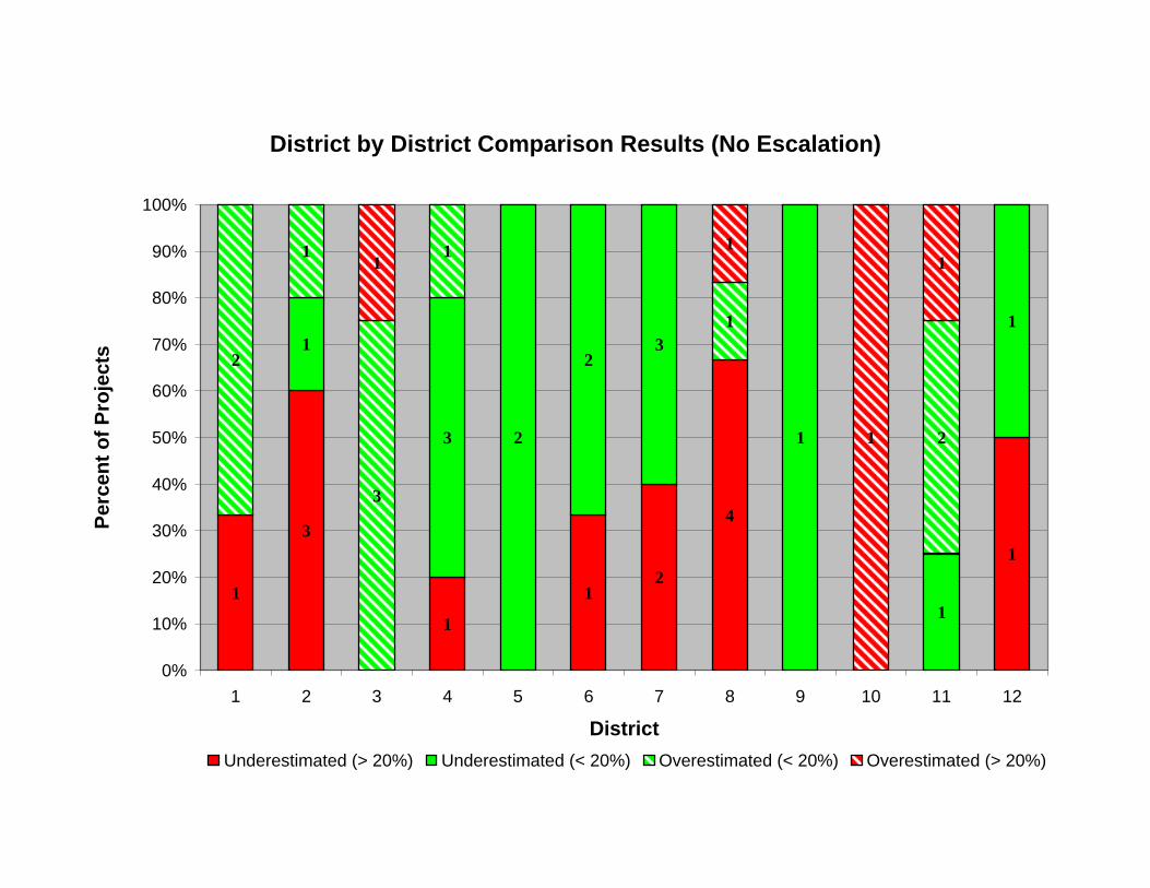
District by District Comparison Results (No Escalation)
1
3
1
12
4
1
1
3 2
23
1
1
1
2
1
3
1
1
2
11
1
1
0%
10%
20%
30%
40%
50%
60%
70%
80%
90%
100%
1 2 3 4 5 6 7 8 9 10 11 12
District
Perc
ent o
f Pro
ject
s
Underestimated (> 20%) Underestimated (< 20%) Overestimated (< 20%) Overestimated (> 20%)

District by District Comparison Results (Escalated 3%)
12
1
1
1
4
1
2
11
1 3
1
1
3
2
1
1
1
1
1 2
1
11
1
11
1 1
0%
10%
20%
30%
40%
50%
60%
70%
80%
90%
100%
1 2 3 4 5 6 7 8 9 10 11 12
District
Perc
ent o
f Pro
ject
s
Underestimated (> 20%) Underestimated (< 20%) Overestimated (< 20%) Overestimated (> 20%)
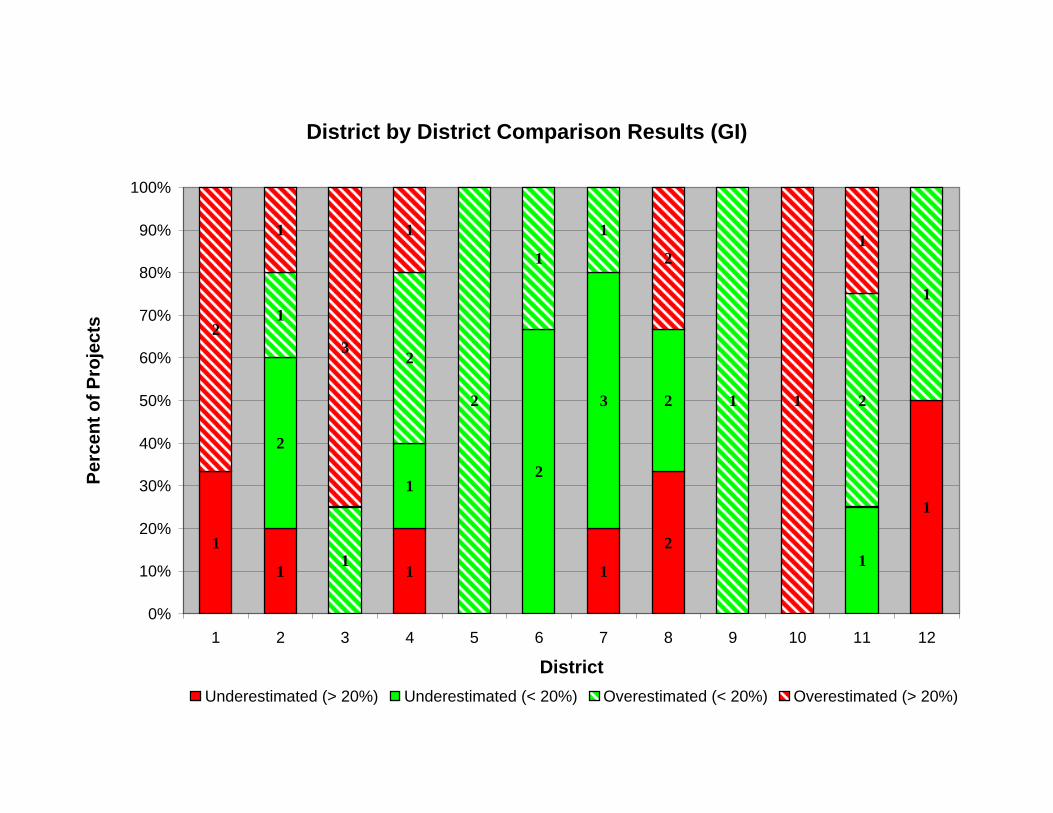
District by District Comparison Results (GI)
1
1 1 1
2
1
2
12
3
11
2
2
1
1
1 2
1
3
2
1
1
2
1
11
2
0%
10%
20%
30%
40%
50%
60%
70%
80%
90%
100%
1 2 3 4 5 6 7 8 9 10 11 12
District
Perc
ent o
f Pro
ject
s
Underestimated (> 20%) Underestimated (< 20%) Overestimated (< 20%) Overestimated (> 20%)

Appendix 4
Cost Category Comparison Charts No Escalation
3 percent Escalation GI Escalation

Cost Category Comparison Results (No Escalation)
55
1
7
2
54
1
1
2
32
21
0%
10%
20%
30%
40%
50%
60%
70%
80%
90%
100%
$1,000,000 to
$1,999,999
$2,000,000 to
$4,999,999
$5,000,000 to
$9,999,999
$10,000,000 to
$25,000,000
Cost Category
Perc
ent o
f Pro
ject
s
Underestimated (> 20%) Underestimated (< 20%) Overestimated (< 20%) Overestimated (> 20%)
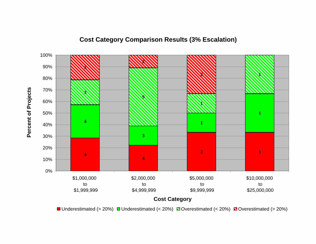
Cost Category Comparison Results (3% Escalation)
44
1
3
1
39
1
2
2
4 1
1
23
0%
10%
20%
30%
40%
50%
60%
70%
80%
90%
100%
$1,000,000 to
$1,999,999
$2,000,000 to
$4,999,999
$5,000,000 to
$9,999,999
$10,000,000 to
$25,000,000
Cost Category
Perc
ent o
f Pro
ject
s
Underestimated (> 20%) Underestimated (< 20%) Overestimated (< 20%) Overestimated (> 20%)

Cost Category Comparison Results (GI)
2 2
14
1
3
71
2
2
5
1
154
0%
10%
20%
30%
40%
50%
60%
70%
80%
90%
100%
$1,000,000 to
$1,999,999
$2,000,000 to
$4,999,999
$5,000,000 to
$9,999,999
$10,000,000 to
$25,000,000
Cost Category
Perc
ent o
f Pro
ject
s
Underestimated (> 20%) Underestimated (< 20%) Overestimated (< 20%) Overestimated (> 20%)

Appendix 5
PID Type Comparison Charts No Escalation
3 percent Escalation GI Escalation

PID Type Results (No Escalation)
1
5
1
14 4
31
24
2
1
44
121
0%
10%
20%
30%
40%
50%
60%
70%
80%
90%
100%
CAPM PR FPSR PPPR PR PSR PSR/PR PSSR
PID Type
Perc
ent o
f Pro
ject
s
Underestimated (> 20%) Underestimated (< 20%) Overestimated (< 20%) Overestimated (> 20%)

PID Type Results (3% Escalation)
1
41
1
52
1 1
14
1
3
5
3
2
33
0%
10%
20%
30%
40%
50%
60%
70%
80%
90%
100%
CAPM PR FPSR PPPR PR PSR PSR/PR PSSR
PID Type
Perc
ent o
f Pro
ject
s
Underestimated (> 20%) Underestimated (< 20%) Overestimated (< 20%) Overestimated (> 20%)

PID Type Results (GI)
1
1
17 1
1 1
14
1
1
24
32
14
41
0%
10%
20%
30%
40%
50%
60%
70%
80%
90%
100%
CAPM PR FPSR PPPR PR PSR PSR/PR PSSR
PID Type
Perc
ent o
f Pro
ject
s
Underestimated (> 20%) Underestimated (< 20%) Overestimated (< 20%) Overestimated (> 20%)

Appendix 6
Elapsed Time Comparison Charts No Escalation
3 percent Escalation GI Escalation

Time Comparison Results (No Escalation)
3
3
5
3
2
3
4
3
3
2
2
2
2 2
1
1
0%
10%
20%
30%
40%
50%
60%
70%
80%
90%
100%
< 6 mos. 7 mos. to
12 mos.
13 mos. to
18 mos.
19 mos. to
24 mos.
25 mos.to
60 mos.
> 60 mos.
Time Between PID and Engineer's Estimates
Perc
ent o
f Pro
ject
s
Underestimated (> 20%) Underestimated (< 20%) Overestimated (< 20%) Overestimated (> 20%)

Time Comparison Results (3% Escalation)
32
4
3
2
1 1
2
3
2
2
2
1
3 5
211
1
0%
10%
20%
30%
40%
50%
60%
70%
80%
90%
100%
< 6 mos. 7 mos. to
12 mos.
13 mos. to
18 mos.
19 mos. to
24 mos.
25 mos. to
60 mos.
> 60 mos.
Time Between PID and Engineer's Estimates
Perc
ent o
f Pro
ject
s
Underestimated (> 20%) Underestimated (< 20%) Overestimated (< 20%) Overestimated (> 20%)
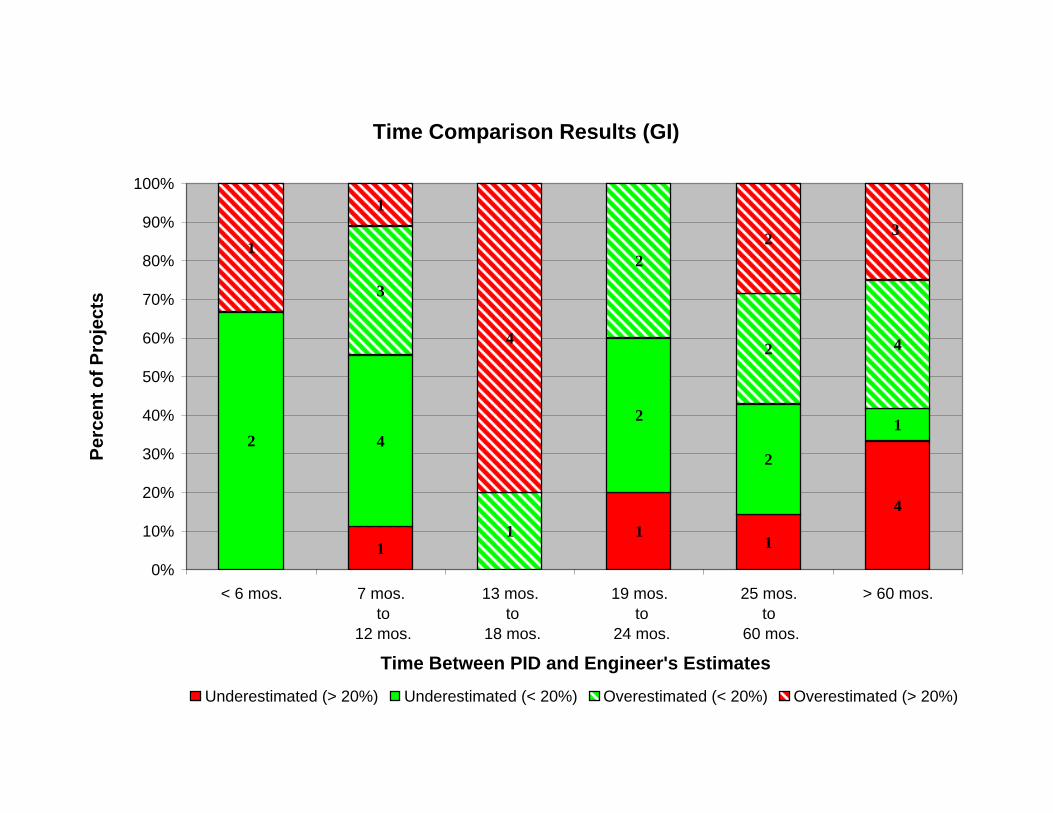
Time Comparison Results (GI)
11
4
42
2
1
3
1
4
1
2
2
2 4
32
1
1
0%
10%
20%
30%
40%
50%
60%
70%
80%
90%
100%
< 6 mos. 7 mos. to
12 mos.
13 mos. to
18 mos.
19 mos. to
24 mos.
25 mos.to
60 mos.
> 60 mos.
Time Between PID and Engineer's Estimates
Perc
ent o
f Pro
ject
s
Underestimated (> 20%) Underestimated (< 20%) Overestimated (< 20%) Overestimated (> 20%)