
Chapter 7 Magnetic Fields. 7.1 THE CREATION OF MAGNETIC FIELDS.
Rep. Prog. Phys., Vol. 46, pp 555-620, 1983. Printed in Great Britain
Planetary magnetic fields
D J Stevenson Division of Geological and Planetary Science, California Institute of Technology, Pasadena, California 91125, USA
Abstract
As a consequence of the smallness of the electronic fine structure constant, the characteristic time scale for the free diffusive decay of a magnetic field in a planetary core is much less than the age of the Solar System, but the characteristic time scale for thermal diffusion is greater than the age of the Solar System. Consequently, primordial fields and permanent magnetism are small a;d the only means of providing a substantial planetary magnetic field is the dynamo process. This requires a large region which is fluid, electrically conducting and maintained in a non-uniform motion that includes a substantial RMS vertical component. The attributes of fluidity and conductivity are readily provided in the deep interiors of all planets and most satellites, either in the form of an Fe alloy with a low eutectic temperature (e.g. Fe-S-0 in terrestrial bodies and satellites) or by the occupation of conduction states in fluid hydrogen or ‘ice’ (H20-NH3-CH4) in giant planets. It is argued that planetary dynamos are almost certainly maintained by convection (compositional and/or ther- mal). If alternative mechanisms such as precessional torques work at all, they only work when they are not needed (i.e. when the core is neutrally or unstably stratified because of other larger energy sources). For any plausible convective vigour, it is possible to satisfy the sufficient conditions of dynamo onset (large magnetic Reynolds number, small Rossby number) for every planet and satellite. Estimates of convective vigour are obtained from estimates of likely energy fluxes and a consideration of the form of convective motions in a rotating fluid sphere. The reason that some planets and probably all satellites do not have dynamos is because the fluid regions of their cores are stably stratified and do not convect. Thermal evolution models indicate that any terrestrial body with an entirely fluid (iron alloy) core becomes stably stratified over geologic time and loses heat by conduction only at the present time. The core energy flux is then totally unavailable for dynamo generation. However, terrestrial bodies that nucleate an inner solid core (e.g. Earth) can usually continue to sustain a dynamo because of the resulting gravitational energy release and compositional buoyancy of convective motions. In contrast, giant planets can easily sustain a dynamo by gradual cooling alone.
The field amplitudes of planetary dynamos are poorly understood. Existing attempts at ‘scaling laws’ are naive because they deny the diversity of planets, and
@ 1983 The Institute of Physics 5 5 5
556 D J Stevenson
poorly constrained because several ‘laws’ perform equally well. Nevertheless, it is possible to assess the likely presence or absence of a dynamo in each planet and satellite, primarily by an analysis of energetic considerations. An interpretation of each Solar-System body is offered and some testable predictions are given.
This review was received in September 1982.
Planetary magnetic fields
Contents
557
1. Introduction 2. The observations
2.1. Basic principles 2.2. Earth 2.3. Jupiter 2.4. Saturn 2.5. Mercury 2.6. Venus 2.7. Moon 2.8. Mars 2.9. Uranus, Neptune and outer Solar-System satellites 2.10. Small bodies and meteorites
3. Composition and evolution of planets 3.1. Basic principles 3.2. Evolution and structure of terrestrial planets 3.3. Evolution and structure of Jupiter and Saturn 3.4. Evolution and structure of Uranus and Neptune
4.1. Non-dynamo sources 4.2. The dynamo problem: kinematic preliminaries 4.3. Fluid motions in planets ( H 4.4. The onset of a convective dynamo (!ow-field limit) 4.5. Finite-field dynamos and scaling laws 4.6. Multipolarity and symmetry 4.7. Time variability and reversals
5 . The synthesis 5.1. Mercury 5.2. Venus 5.3. Earth 5.4. Moon 5.5. Mars 5.6. Jupiter 5.7. Saturn 5.8. Uranus and Neptune 5.9. Pluto and giant planet satellites
6. The future Acknowledgments References
4. The sources of planetary magnetism
0 )
Page 559 561 561 563 564 565 566 566 567 567 567 568 568 568 570 581 583 5 84 5 84 587 593 598 601 605 607 608 608 609 61 1 612 613 613 614 615 616 616 617 617
Planetary magnetic fields 5 5 9
1. Introduction
Magnetic fields are ubiquitous in the Universe because of the abundance of free electric charges and the absence or relative scarcity of free magnetic monopoles. On the astrophysical scale, magnetic fields are a consequence of large-scale currents and the cause of complex motions of plasma. We are also familiar with magnetic fields on the human length scale, often associated with permanent magnetism and caused by microscopic currents. In view of the existence of magnetic fields on length scales as diverse as centimetres and light years, one’s first inclination is to be unsurprised by the existence of substantial magnetic fields associated with planets, which have a size halfway between centimetres and light years on a logarithmic scale. In fact, the persistence of large planetary magnetic fields is far from obvious and their explanation provides insights into the structure and dynamics of a planetary interior.
The existence of large planetary magnetic fields is not immediately obvious because planets are too large (and hence too warm internally) to preserve much of the microscopic magnetism of permanently magnetised material, yet too small to sustain primordial magnetic fields in the non-magnetic conducting materials for the age of the Solar System. A non-magnetic m’aterial is one in which there is no possibility of spontaneous magnetisation and the magnetic field is equal to the magnetic induction (except for a constant dependent on the choice of units). Ohm’s law, Ampbre’s circuit law and Faraday’s law of induction are then respectively
j = a E + - x H i P > 41r V x H = - j
C
1 aH V x E + - - = 0 c at (1.3)
(Gaussian units) where j is the current density, CT is the electrical conductivity, E is the electric field, H is the magnetic field, V is the velocity field of the conductor relative to the frame in which the fields are measured, and c is the velocity of light. Displacement currents are neglected because we are interested in phenomena with characteristic time scales much longer than the light travel time. Deviations from Ohm’s law are potentially significant but are neglected for the moment. Elimination of E and j yields
aH - = A V ~ H +V x (V x H ) at (1.4)
where A = c2/41ra (assumed constant) is called the magnetic diffusivity and V H = 0 has been assumed (i.e. no magnetic monopoles. If the recent tentative detection of a monopole by Cabrera (1982) is correct then the equations require modification.)
Suppose that one formed an electrically conducting planet at time t = 0 with an initial permeating field -Ho, this field being derived from some ‘external’ source such
560 D J Stevenson
as the interstellar medium or the primordial solar nebula. If the external source is removed and the body is subsequently internally inactive ( V = 0) then equation (1.4) predicts a diffusive decay of the field H - Ho exp (-f/7), where T = R2/ r2A and R is the planetary radius (also the characteristic length scale of the field: IV2H( - H/R2) . The characteristic atomic unit of electrical conductivity is e 2 / a o h (e is the electron charge, a. is the first Bohr radius, h is Planck's constant divided by 27r) so that A - cuG2(h/m) - lo4 cm2 s-', where afs is the fine structure constant and m is the electron mass. It follows that the magnetic diffusion time 7mag- (3000 yr)(R/103 km)2, much less than 4.5 x l o9 yr, the age of the Solar System. Even in the case of Jupiter, where A is somewhat smaller and R is large, T , , ~ is at most a few hundred million years. Primordial fields are thus almost certainly unimportant in the non-magnetic constituents of planets.
In contrast, the thermal diffusion time is long. Application of the Wiedemann- Franz relationship (discussed in any elementary solid-state physics text, e.g. Ashcroft and Mermin (1976)) leads to the estimate K - 10(aokBT/e2)(h/m) -0.1 cm2 s-' for the thermal diffusivity of a metal, where T is the temperature and kB is Roltzmann's constant. Notice that K<<A, primarily because the fine structure constant is small (but also because thermal energies are much less than atomic energies). The thermal diffusion equation aT/Jt = KV2T has an associated characteristic decay time 7 t h = R 2 / r 2 K - (3 x 10' yr)(R/103 km)2. The time scale is even longer if the thermal diffusivity of an insulator cm2 s-') is used. Since planets possess large internal heat sources (radiogenic in the terrestrial planets, gravitational in the giant planets), high internal temperatures are unavoidable. The temperature is stabilised by convec- tion (which occurs almost everywhere within most planets) but this stabilised value far exceeds the Curie point of ferromagnetic materials. Only the near-surface (crustal) materials of terrestrial planets possess permanent magnetism; the resulting magnetic field is orders of magnitude smaller than the 0.5 G surface field characterising the Earth but is important for bodies where the field is much smaller than the terrestrial field.
However, equation (1.4) admits the possibility of sustaining a field indefinitely by virtue of the induction term V x ( V X H). The ratio of this term to the diffusion term h V 2 H is of the order of the magnetic Reynolds number defined as R M = VL/A where V and L are characteristic magnitudes for the velocity field and the length scales of the magnetic-field variation, respectively. If RM 3 1, then one could imagine a solution to equation (1.4) in which Ohmic diffusion is balanced by induction and aH/at is zero or has a non-negative average value. In fact, the necessary (but not sufficient) condition for this to happen is closer to R M a 10. This state is called a dynamo and equation (1.4) is often referred to as the dynamo equation. Extensive treatments of dynamo theory can be found in Moffatt (1978) and Parker (1979). Other recent reviews include Gubbins (1974) and Levy (1976). A dynamo requires that the characteristic time scale of the fluid motions, L/ V, be much less than T , ~ ~ which, as we have already shown, is much less than the age of the Solar System. Thus, a dynamo is not likely to retain memory of the initial 'seed' field responsible for its establishment.
The essential physical idea of a dynamo is that the motion of the medium in the presence of a magnetic field generates electric currents with associated fields that augment the original field. The regeneration is required to offset the effects of Ohmic dissipation. This motion is necessarily doing work (the magnetic field may impede the flow) and some energy source must be available to sustain the motion. Further- more, not just any motion in which R M a 10 is capable of sustaining a dynamo. The
Planetary magnetic fields 561
area of research known as kinematic dynamo theory is concerned with establishing and characterising the nature of velocity fields capable of dynamo generation. For example, rotation (either uniform or differential) is not sufficient by itself.
The full dynamic problem involves simultaneous solution of the dynamo equation with the equation of motion (the hydromagnetic Navier-Stokes equation). This problem is extremely difficult, but one conclusion seems reasonably certain: thermally or compositionally driven convection in a low-viscosity rotating fluid can sustain a dynamo provided 60th R M + 10 and the Coriolis force is dynamically important. In practice, the latter can be expressed as Ro 6 1 where Ro = V/2RL and R is the spin angular velocity of the planet. In principle, all of the planets and large satellites are capable of satisfying R M ? a 10 and Ro6 1. In practice, many of them may not have dynamos, even when they possess fluid regions of large radial extent, because of the absence of convection, or the weakness of fluid motions. Sources of motion other than convection are possible, although less likely to be important, and are discussed in 8 4.
Solids can also flow and this motion is responsible for continental drift on Earth. However, these motions are much too slow (-lo-’ cm s-*) to provide RMa 10, even if the medium were a good metal. (These motions are also too viscous for the Coriolis effect to be important.)
A much more difficult issue concerns the expected amplitude of a dynamo magnetic field. Estimates are established in § 4 which are sufficient in most cases to identify whether an observed field is likely to be the consequence of dynamo generation. However, there is no predictive theory for field amplitudes and this is an unfortunate limitation on the interpretation of planetary data.
With this limited understanding, it is nevertheless possible to use the measured magnetic field of a planet as a probe of the thermal, electronic and dynamic state of its deep interior. The relevant observations now exist for all but the outermost three planets and for three large satellites (the Moon, Io and Titan). Three planets clearly possess dynamos (Earth, Jupiter, Saturn), one planet probably possesses a dynamo (Mercury) and the evidence for the remaining bodies is either non-existent or best interpreted as the absence of a dynamo. (Uranus may have a dynamo, but the evidence is a few enigmatic radio bursts rather than a clear indication of a substantial magnetic field.) In this review I propose to synthesise these observations with current knowledge of the composition and evolution of planets and the sources of planetary magnetism. Satellites are considered also, because many are large enough to have interiors which are very different from the surface or near-surface environments. In 8 5 , I offer a preferred interpretation or prediction for each planet or large satellite in the Solar System. This is a risky venture in view of the existing limitations in both theory and observation, but it is my hope that this effort and the logic which precedes it will help dispel the common prejudices that dynamo theory lacks teeth and that planetary magnetic-field interpretation is largely speculation.
2. The observations
2.1. Basic principles
Since V H = 0, it is always possible to represent the magnetic field in terms of two scalar fields. If the current is zero (V x H = 0) as well, in the region where observations
562 D J Stevenson
are being made, then H can be represented as the gradient of a potential 4. In the spherical geometry appropriate to planets it is natural to separate 4 into the contribu- tions from internal and external sources and expand in spherical harmonics:
m l I
P;"(cos 4)(G;" cos mcp +H;" sin mcp) f = 1 m=O
(2.4)
where R is the equatorial planetary radius, r is the radial coordinate, 6 is the colatitude, cp is the longitude, P;" are the associated Legendre functions (usually chosen to be Schmidt-normalised) and the coefficients g;", h;", G;", H;" are determined by observa- tion. In view of the tendency for magnetic fields to exhibit some rotational symmetry, it is convenient and physically appropriate to choose 6 = 0 as the rotational axis of the planet. It is important to realise, however, that the field representation is a mathematical construct: somewhat arbitrary and infinitely flexible. There is sometimes an unfortunate tendency to isolate some aspect of a particular representation and attribute special physical significance to it. Unless there is independent evidence to support this procedure, the resulting inferences should be viewed with skepticism. An example of a possibly artificial distinction is the notion that dipole terms ( I = 1 in equation (2.3)) have a different physical cause than higher-order terms ( I 3 2). On the other hand, it is possible from symmetry arguments that even-l terms behave differently from odd-l terms.
The most misleading statement frequently made about planets is that they possess dipole magnetic fields. Since the dipole components decay least rapidly at large r , they must dominate if one's observation point is far removed from the source. It is a denial of post-Newtonian scientific philosophy to attribute greater significance to the dipole terms simply because they are largest at the point of observation. In fact, higher-order terms are comparable at the surface of the source region (the core). Nevertheless, the dipole moment M defined by
is the most frequently quoted quantitative measure of a planetary magnetic field and higher-order moments are poorly determined for all planets other than the Earth.
Measurements at the Earth's surface and by orbiting spacecraft have provided values of g;", h;" to 1 = 12, although errors are large beyond 1 = 8 (Barraclough 1981). Venus and the Moon have had their magnetic fields characterised by orbiting space- craft, while the magnetic environments of Mercury, Mars, Jupiter and Saturn have been sampled only by flyby spacecraft. In every case except the Earth, the data are strictly incomplete for a rigorous determination of even the lowest harmonics of Gi. In practice, however, the determination of the dipole moment (or its upper bound) and sometimes its tilt are reasonably well posed for these bodies, even from a single flyby. The analysis of incomplete data sets is a difficult problem and will not be dealt with here (but see, for example, Shure et a1 1982). Flyby data are sufficiently
Planetary magnetic fields 563
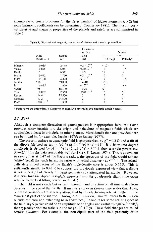
incomplete to create problems for the determination of higher moments ( l a 2 ) but some harmonic coefficients can be determined (Connerney 1981). The most import- ant physical and magnetic properties of the planets and satellites are summarised in table 1.
Table 1. Physical and magnetic properties of planets and some large satellites.
Equatorial surface Dipole
Mass Radius field (Earth = 1) (km) (GI Tilt (deg) Polarityf
Mercury Venus Earth Moon Mars Jupiter Io Saturn Titan Uranus Neptune Pluto
0.055 0.815 1
0.012 0.108
0.015
0.022
318
95
14.6 17.2
-2 x
2 440 6 051 6 371 1760 3 390
69 800 1810
58 400 2 560
25 500 24 500 -1 500
-2 x 6 2 x 10 -~
s 2 x 10⁻⁶
4-10 s 10-2
0.21 ~3 x
? ?
0.3
9
-lo? ?
11 ? ?
-10 ?
<1 ? ? ? ?
+?
? + ? + - ? + ? ? ? Q
f Positive means approximate alignment of angular momentum and magnetic-dipole vectors.
2.2. Earth
Although a complete discussion of geomagnetism is inappropriate here, the Earth provides many insights into the origin and behaviour of magnetic fields which are applicable, at least in principle, to other planets. More details than are provided here can be found in, for example, Jacobs (1975) or Stacey (1977).
The present surface geomagnetic field is characterised by g? = 0.3 G and a tilt of the dipole (defined as tan-’{[(g:)2+(l;i:)2]*’’/g~}) of -11”. If a harmonic degree amplitude is defined by A: = (I + 1) [(g;“)’+ (h;“)’], then a single power law A I - 2.1-‘ fits the data reasonably well for 1 G 1s 8 (Lowes 1974). This is equivalent to saying that at 0.47 of the Earth’s radius, the spectrum of the field would appear ‘white’ (recall that each harmonic varies with radial distance r as r-(’+’)). The seismi- cally determined radius of the Earth’s high-density core is about 0.55 R. This is sufficiently similar to 0.47 R to support the previously expressed view that a dipole is not ‘special,’ but merely the least geometrically attenuated harmonic. (However, it is true that the dipole is slightly enhanced and the quadrupole slightly depressed relative to the best fitting power law for A,.)
The field is not steady but varies in strength and direction on all time scales from decades to the age of the Earth. (It may vary on even shorter time scales than 10 yr, but these variations are severely attenuated by the electromagnetic skin effect in the lowermost part of the mantle. Throughout this review, ‘mantle’ refers to the region outside the core and extending to near-surface.) If one takes some scalar aspect of the field, say S (which could be an amplitude or an angle), and evaluates T~ lS/(dS/dt)l, then typically this time scale is in the range 102-104 yr. These field changes are called secular variation. For example, the non-dipole part of the field presently drifts
564 D J Stevenson
westward at 0.2” of longitude per year, corresponding to 1800yr for a complete revolution relative to the frame of reference defined by the rotation of the Earth’s mantle. We can convert this into an equivalent averaged velocity V, E n-Rc/r,, where R , is the core radius. For the westward drift of the non-dipole field, V, = 0.02 cm s-’, For a magnetic diffusivity A = 2 x lo4 cmz s-’; RM= V,R,/A -- 350. It should be stressed, however, that we cannot necessarily interpret V, as a fluid velocity, since the motion of field lines may occur by diffusion or as a consequence of wave propagation. Nevertheless, these ‘velocities’ constitute a measure of core dynamics. More precise information on possible velocities can be obtained (e.g. Benton 1979, Whaler 1980) by focusing on special regions of the core-mantle boundary and assuming ‘frozen flux’ (i.e. no Ohmic diffusion on the time scale of observation). These analyses suggest that upwelling motions are weak (s cm s-’) when averaged over large (&lo6 km2) regions of the core-mantle boundary.
Paleomagnetism (measurements of the magnetisation of rocks) provides informa- tion on previous field orientations and some very limited information on previous field strengths. Repeated alternations of magnetic polarity in a series of lava flows or sedimentary layers indicate that the Earth’s field reverses aperiodically. The process is stochastic, with the current reversal rate being a few times per million years, but this rate has varied greatly over geologic time (McElhinny 1971). Analysis of the normal and reversed polarity states indicate that they have different behaviour (Merrill et ai 1979). This is an astonishing result because all of the equations describing the geodynamo are unchanged if H is replaced by -H. The actual reversal of the magnetic field occurs on a much shorter time scale (-a few thousand years) than the time between reversals, and there are also many fluctuations on this dynamic time scale which could be characterised as ‘excursions’ or ‘aborted reversals’ (Hoffman 1981). Despite this complex behaviour, the time-averaged field for the last twenty million years is aligned with the Earth’s rotation axis (data reviewed by McElhinny (1973)). This very important result leads to the ‘axial dipole hypothesis’ which asserts that this behaviour persists for all geologic time, and enables paleomagneticians to recon- struct, at least partially, the past motions of continents relative to the axis of rotation. The apparent validity of the axial dipole hypothesis is a clear indication of the role of rotation in the geodynamo.
Indications of a geomagnetic field are found in rocks as old as 3 . 5 ~ 109yr (McElhinny and Senanayake 1980) and the paleofield strength was comparable to the present field. The picture which emerges is thus one of a geodynamo which has existed in a similar form to the present for probably the entire history of the Earth and yet is dynamically active and complex on much shorter time scales.
2.3. Jupiter
The Jovian field is the best studied planetary dynamo other than the Earth. Radio emissions associated with accelerated particles in the Jovian magnetosphere were detected serendipitously in 1955 at a frequency of 22.2MHz (Burke and Franklin 1955) and subsequent extensive observations of non-thermal emission have been reviewed by Berge and Gulkis (1976). By the late 1960s, the approximate magnitude, tilt and polarity (opposite to that of the Earth) of the magnetic dipole were already deduced. Radio periodicity also provides an accurate rotation rate for the field and thus the planetary interior. However, the flybys of four spacecraft in the 1970s provided direct magnetic-field determinations of a quality and quantity that can never
Planetary magnetic fields 565
be achieved by the indirect techniques of ground-based observations. Pioneer 10 flew by Jupiter in December 1973 with a closest approach distance of 2.9 Jovian radii (2.9 Rj) from the ceztre of the planet (1 R J = 7 1 400 km at the equator); Pioneer 11 approached within 1.6 R J in December 1974; Voyager 1 to 4.9 R J in March 1979; and Voyager 2 to 10 R j in July 1979. The Pioneer 10 and 11 spacecraft are equipped with helium vector magnetometers and Pioneer 11 and both the Voyager spacecraft are equipped with fluxgate magnetometers. The data from Pioneer 11 are the best for determining the internal field, not only because of the close approach but also because of good latitude and longitude coverage. Initial disagreements between the two data sets from the two onboard magnetometers were eventually resolved (Acufia and Ness 1976, Smith et a1 1976) and reasonably consistent (though far from complete) models of the field have emerged. Similar models have been obtained from Voyager data (Connerney et a1 1982a).
These models are characterised by a dipole moment of about 4.2 G R:, a dipole tilt of about 10" and large higher-order terms. The ratios dipole : quadrupole : octupole are about 1.00 : 0.25 : 0.20 for Jupiter compared with 1-00: 0.14 : 0.10 for the Earth. If we use our previous discussion of the Earth as a guide, this result suggests that the region of field generation in Jupiter is far more extensive, reaching at least as far as 0.75-0.8 R J (Elphic and Russell 1978). The significance of this will become more apparent in subsequent sections. Although the data clearly require the high-order multipoles, their quantitative determinations are difficult because of the inherent ambiguities in flyby data and the possible contributions of unmodelled external currents. It is not yet possible, therefore, to use the existing spacecraft data sets to determine time variation in the intrinsic field on a time scale of years (Connerney and Acuiia 1982). Secular variation has not been detected yet for any planet other than the Earth. It would also be interesting to know how 'rich' is the magnetic-field spectrum of Jupiter. It has been speculated that 'spots' of high field exist (Stevenson 1976) but their existence would not be resolvable except by global measurements at the atmospheric level. Russell (1980) provides more detail on the current quantitative understanding of the Jovian field.
2.4. Saturn
Like Jupiter and Earth, Saturn emits kilometric and hectometric radiation (Kaiser et a1 1980). Since the peak of the spectrum of Saturn's emissions is about one-eighth the frequency of the corresponding Jovian peak, a correspondingly smaller field of 0.5-1 G was expected at Saturn. When Pioneer 11 arrived in September 1979, and approached within 1.35 R,, it detected an even smaller dipole of about 0.21 G R? (where 1 R s = 60 000 km). The major surprise of this flyby was the extreme smallness of the dipole tilt of 61' (Smith et al 1980), in contrast to the values of 10-11" which characterise Earth and Jupiter. Indeed, the tilt is so small that it was not possible to detect the rotation rate of Saturn from magnetometer measurements. The field was also inferred to be very nearly dipolar with a dipo1e:quadrupole ratio of perhaps 1 : 0.12 (but see below).
As Voyager 1 approached Saturn in January 1980, it detected modulated kilometric radio emissions, from which a rotation period of 10h39.4" is deduced (Desch and Kaiser 1981). Clearly, the Saturnian field is not exactly symmetric about the rotation axis. Nevertheless, analyses of the flybys of Voyager 1 (November 1980, at 3.1 R,) by Ness et a1 (1981) and Voyager 2 (August 1981, at 2.7 R,) by Ness et al (1982)
566 D J Stevenson
continue to show very little evidence for a dipole tilt. A very recent analysis (Connerney et a1 1982b) indicates that the combined data sets can be represented by an axisym- metric field (dipole tilt E 0), provided substantial axial quadrupole and octupole com- ponents are included in the analysis (larger than Smith et a1 (1980)). The possible significance of this startling result is considered in 08 4 and 5. For the moment, it is sufficient to note that if planet dipoles ‘wander’ in a way similar to Earth’s dipole, then the probability of finding a chance alignment of rotation axis and dipole axis to within an angle E (expressed in degrees) is about e 2 , It seems likely, therefore, that Saturn’s small or non-existent dipole tilt is not by chance. It is not known what asymmetry (if any) is needed to explain the radio observations.
2.5. Mercury
Aside from Earth, Jupiter and Saturn, Mercury is the only other planet for which in situ measurements indicate a field large enough to probably require a dynamo. Mercury has been visited by only one spacecraft, Mariner 10, which made three flybys in 1974-75. The first and last of these flybys were within about 700 km of the surface and useful for determining the intrinsic field (Ness et a1 1976). The maximum fields observed in these two passages were 0.001 G and 0.004 G, only about one order of magnitude higher than the interplanetary field during and after closest approach. Consequently, the Mercurian field can not be characterised with as much precision and certainty as the previous cases discussed. In particular, the inferred internal field depends to some extent on the modelling of the magnetosphere and solar-wind effects (Slavin and Holzer 1979). Their conclusion for the dipole moment is ( 4 * 1 . 5 ) ~ lop3 G R L where 1 RM=2440 km. The data are not adequate for determinations of dipole tilt and higher multipoles but appear to require either or both (e.g. dipole tilt - lo”, quadrupole :dipole - 0.5 : 1 are possible). There is no question that a proper characterisation of the Mercurian field requires another mission.
2.6. Venus
Seven missions to Venus have carried magnetometers, beginning with Mariner 2 in 1962 and extending to the Pioneer Venus orbiter which arrived in late 1978. Even with Mariner 2, which approached to within only 6.6 R, (where R,=6051 km), it was apparent that the magnetic field is much less than Earth’s field. The upper bound to the intrinsic Venus magnetic dipole has been progressively reduced and is now about 2 x G R?, based on the Pioneer Venus data (Russell et a1 1980). These authors effectively discount the interpretation of Dolginov et a1 (1978) of Soviet Venera data which might indicate a field about one order of magnitude larger but are questionable because the Venera spacecraft were not tracked continuously and often had uncertain orientation of the measurement platform.
Analysis of the Pioneer Venus orbiter data indicates field variations which do not persist from orbit to orbit and do not resemble any simple solar-wind interaction with an intrinsic planetary field. Knudsen et a1 (1982) suggest an intrinsic dipole of 3 x G R? but this is model-dependent. The importance of establishing the magni- tude of the intrinsic field remains high because the current estimates are now at the level where a variety of interesting and geophysically significant non-dynamo contribu- tions (crustal magnetisation, induced internal currents) might be detectable. However, it is clear that Venus does not possess a dynamo.
Planetary magnetic fields 567
2.7. Moon
Luna 2 carried out the first lunar magnetic-field measurements in 1959. Subsequent Soviet and US orbiters, especially the ‘subsatellites’ placed in orbit on the Apollo 15 and 16 missions, have progressively reduced the upper bound to the global dipole moment (reviewed by Russell (1980)). The current upper bound is 2 x lop6 G Rh, where 1 R M = 1760 km. In contrast, the magnetometers at the Apollo landing sites measured local fields that were typically two and occasionally three orders of magnitude greater. These fields are generally associated with small-scale features and often vary markedly over distances of a few kilometres. Some large-scale magnetic anomalies are detectable from orbit and appear to be associated with thin, highly magnetised layers deposited during the impact of a large meteorite or comet (see Hood (1981) for a review of these data). It is also possible that a globally magnetised crust, disrupted by impacts and reoriented by polar wander, could provide the observed magnetic anomalies (Runcorn 1982). This hypothesis follows from the conjecture that the Moon once possessed a large dynamo-generated magnetic field.
The large, stable remanent magnetisations of returned lunar rocks are consistent with (but do not demand) a large lunar paleofield. The measurements of lunar paleointensity remain controversial but suggest that the lunar field decayed exponen- tially from -1 G at 4.0 x lo9 yr bp (before present) to -0.05 G at 3.2X lo9 yr bp (Stephenson et a1 1975). As we shall see later, the interpretation of these data in terms of a dynamo presents several difficulties. Even though we have more information for the Moon than any other extraterrestrial body, another mission (a polar orbiter) may be needed to resolve the puzzles posed by the existing data (Hood 1981).
2.8. Mars Many spacecraft have been to Mars, but only four (Mariner 4, Mars 2 , 4 and 5) carried magnetometers and the data obtained do not provide a compelling case for an intrinsic magnetic field (Russell 1979b). The data obtained by Mars 3 and 5 have been interpreted by Dolginov (1978a, b) as evidence for a dipole of about 3 x G R’, (where 1 R M = 3390 km) but Russell finds that the data also appear to be consistent with the draping of interplanetary magnetic-field lines around an obstacle. A reason- able upper bound to the magnetic dipole is then G RL. The controversy exists in part because there are no nightside magnetosphere measurements, and will not be fully resolved unless another mission is carried out. The Viking retarding potential analyser data have been interpreted as suggesting a small permanent field (Cragin et a1 1982). In any event, it is clear that any intrinsic field is at most comparable to the crustal permanent magnetisation of the Earth and no active dynamo is indicated:
2.9. Uranus, Neptune and outer Solar-System satellites
Radio emissions may have been detected from Uranus (Brown 1976) by the Imp 6 satellite in Earth orbit, but it is possible that the emissions were terrestrial. Recent observations of intense Lycr emissions from Uranus (Durrance and Moos 1982) suggest the presence of a magnetosphere. Uranus will be reached by Voyager 2 in 1986 and we will probably have to wait until then for information on the Uranian field. No detection of radio bursts has been claimed for Neptune and the existing radio spectra for these two planets do not provide any useful constraint on their magnetic environments.
568 D J Stevenson
A number of the outer Solar-System satellites are large enough to be considered as planets: the Galilean satellites (Io, Europa, Ganymede, Callisto), the large Saturnian satellite Titan and the large Neptunian satellite Triton all have comparable radii to Mercury or the Earth’s moon. Pluto, with a radius of about 1500 km, is also in this category. Two of these bodies (Io and Titan) have been approached close enough for some useful statement to be made about their intrinsic magnetic fields. Io was approached to within 20 000 km by Voyager 1 and the observed field perturbations were tentatively interpreted by Kivelson et a1 (1979) as evidence for an intrinsic magnetic dipole of about IO-* G R:, where R I = 1810 km. Although this is larger than the Mercurian field, the identification is much less secure because the local magnetic environment (the magnetosphere of Jupiter) is almost as intense as the proposed intrinsic field of Io. In these circumstances, the interpretation is necessarily dependent on model assumptions for the subsonic flow of Jovian plasma past Io, and the form of magnetic-field line reconnections. Ganymede was approached to within 63 000 km by Voyager 2 and no evidence of an intrinsic field was found (Burlaga et a1 1980) but this encounter was too distant to exclude the possibility of a substantial Ganymedean field. However, Voyager 1 did approach to within 6500 km of the centre of Titan and an upper bound of 3 x G R ; (where Rr = 2570 km) was established for the dipole (Ness et a1 1981).
2.10. Small bodies and meteorites
Meteorites are believed to be derived from the break-up and dissemination of larger bodies, up to -100 km in radius. They frequently include magnetised material, but the origin of this magnetism is difficult to pinpoint (Brecher 1977). Differentiated meteorites (e.g. iron meteorites) have magnetisations that have been produced or altered by brecciation, metamorphism and shock processes. Only the relatively unmodified and volatile-rich carbonaceous chondrites show clear evidence for an ambient magnetic field of up to 1 G during formation. Since these meteorites were probably not part of bodies which differentiated and formed iron cores, it is unlikely that this ambient field is of internal origin. The field is more probably intrinsic to the solar nebula or gaseous environment in which these meteorites formed.
3. Composition and evolution of planets
3.1. Basic principles
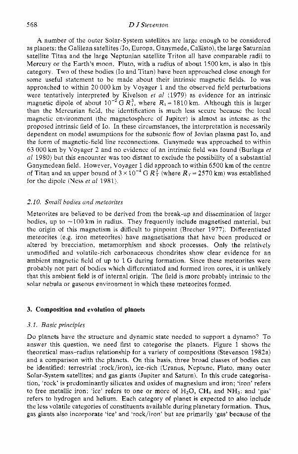
D o planets have the structure and dynamic state needed to support a dynamo? To answer this question, we need first to categorise the planets. Figure 1 shows the theoretical mass-radius relationship for a variety of compositions (Stevenson 1982a) and a comparison with the planets. On this basis, three broad classes of bodies can be identified: terrestrial (rock/iron), ice-rich (Uranus, Neptune, Pluto, many outer Solar-System satellites) and gas giants (Jupiter and Saturn). In this crude categorisa- tion, ‘rock’ is predominantly silicates and oxides of magnesium and iron; ‘iron’ refers to free metallic iron; ‘ice’ refers to one or more of H 2 0 , CH4 and NH3; and ‘gas’ refers to hydrogen and helium. Each category of planet is expected to also include the less volatile categories of constituents available during planetary formation. Thus, gas giants also incorporate ‘ice’ and ‘rock/iron’ but are primarily ‘gas’ because of the
Planetary magnetic fields 569
Figure 1. Average densities of planets and their dependence on mass. The ‘terrestrial’ curve is for bodies of the same composition as the Earth; the ‘ice-rich’ curve is for a body that incorporates HzO, CH4 and NH3 in cosmic abundance (in addition to the ‘rock’ component), and the ‘cosmic’ curve is for cold (T = 0 K) bodies of cosmic composition. The broken curve is a cosmic composition body with internal temperatures appropriate to Jupiter and Saturn. In order moving outwards from the Sun, the planets are represented by the symbols Me, V, E, Ma, J, S, U and N. I refers to Io, LI refers to large icy satellites (Ganymede, Callisto, Titan).
greater cosmic abundances of hydrogen and helium. Uranus and Neptune also incor- porate all categories of constituents but never retained the cosmic component of gas. Nevertheless, they incorporated enough gas to reduce their average densities below those appropriate for purely ‘ice’ bodies. The terrestrial planets contain extremely small quantities of ice and gas.
A necessary condition for a dynamo is a large, electrically conducting fluid region in non-uniform motion. There are consequently three aspects to consider: the existence of a conducting region; the fluidity of this region; and the existence of energy sources to drive non-uniform motions in this fluid.
High conductivity can be achieved in two ways. It can result either from the existence of an abundant ‘conventional’ metal (i.e. an element or compound which is a metal under normal, low-pressure conditions) or from the pressure-induced metalli- sation of a constituent that is normally insulating. Among the ten most abundant elements in the Universe or the Solar System, only iron is commonly found in a metallic form at low pressures. Magnesium is the only elemental metal more abundant than iron, but magnesium is invariably combined with silicon and oxygen under the conditions prevailing during and after planetary formation. Silicates also incorporate some iron, but most of the dense metallic iron is ‘free’ and available to form a core. However, all normally non-conducting materials eventually become metals if sub- jected to sufficient pressure, so it is by no means obvious that iron cores are the expected source region of magnetic fields.
Pressure metallisation occurs because the Pauli exclusion principle, together with the Heisenberg uncertainty principle, imposes a premium on localised electronic states when the density is high. Eventually, it is always energetically favourable to delocalise electronic states, forming a metallic state. The work done achieving this state is -PV - A E where P is the required pressure, V is the volume per atom or molecule
570 D J Stevenson
(typically -loa: where a. = 0.529 x lo-* cm is the first Bohr radius) and AE is a characteristic electronic band gap energy (-a few electron volts). The necessary pressure is then typically a few megabars (1 eV/a: = l O I 3 dyn cm-’ = 10 Mbar). (There may be counterexamples to this simple picture; e.g. McMahan and Albers (1982).) A consequence of hydrostatic equilibrium is that a characteristic internal pressure, Pi, in a planet is pgR where p is the average planetary density, g is the gravitational acceleration and R is the radius. This can be expressed as
P i z 2 . 5 ( - ) ’I3( - ! ) 4/3 Mbar Mo Po (3.1)
where M is the planetary mass and the subscript 0 refers to the Earth. Since 2.5 Mbar is typical for a metallisation pressure, we might expect that the deep interiors of all planets at least as massive as the Earth are metallic, regardless of whether iron is present. Smaller bodies (including the terrestrial planets Mars and Mercury) would only have metallic cores to the extent that they incorporated iron. In fact, pressure metallisation is unquestionably important in only two planets (Jupiter, Saturn), where hydrogen is metallised. It is also probably important in Uranus and Neptune, where water may be metallised.
The fluidity of the metallic region depends primarily on composition and secondly on the thermal evolution of the planet. In terrestrial planets, where a likely structure is an iron core overlaid by a silicate mantle, the partial fluidity of the core depends crucially on the existence of alloying constituent(s) capable of substantially reducing the freezing point of iron. This important conclusion (described in much greater detail below) rests on two principles, The first is that the mantle undergoes solid-state convection and self-regulates at a temperature substantially below the melting point of its major mineral phases. The second principle is that the melting points of iron and of the major silicate and oxide phases are very similar, even at high (megabar) pressures. Of course, fluidity then requires that the self-regulated mantle temperature be at least as high as the minimal melting point (the eutectic) of the iron alloy. This requirement is almost certainly satisfied in all terrestrial planets.
In contrast, the four large outer planets have internal temperatures well in excess of the freezing points of gaseous or icy constituents. This fact reflects a fundamental distinction between terrestrial and outer planets. In terrestrial planets, the major constituents are highly subcritical in the thermodynamic sense (i.e. these planets possess solid surfaces). In the large outer planets, the major constituents are super- critical (i.e. these planets possess ‘bottomless’ atmospheres).
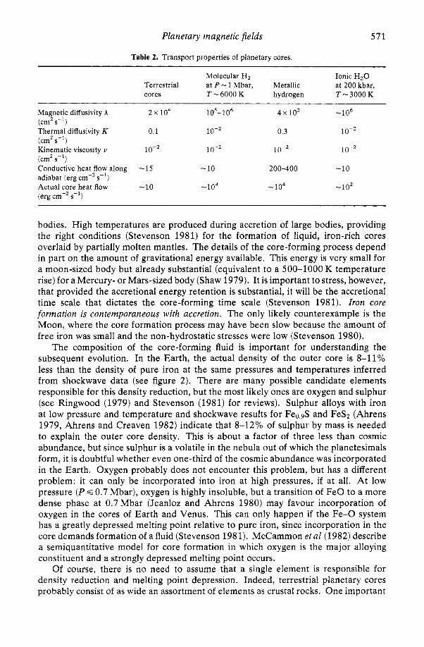
The existence of energy sources capable of driving the non-uniform flows needed for a dynamo is the most difficult problem in planetary modelling. In the terrestrial planets, it is argued below that purely thermal convection may not operate in present- day liquid iron cores but that compositionally driven convection associated with a progressively freezing inner solid core operates in Earth and Mercury. In the large outer planets, thermal convection is almost certainly present and predictions of the dynamic state can actually be made with greater confidence than for the terrestrial planets. Table 2 summaries the important transport properties of planetary cores.
3.2. Evolution and structure of terrestrial planets
The most likely formation scenario for the terrestrial planets (Safronov 1972, Wetherill 1980) leads to efficient mixing of particulate silicates and free iron, at least in small
Planetary magnetic fields 571
Table 2. Transport properties of planetary cores
Molecular H2 Ionic H20 Terrestrial at P - 1 Mbar, Metallic at 200 kbar, cores T - 6000 K hydrogen T-3000K
Magnetic diffusivity A 2~ io4 io5- io6 4x10' -lo6 (em's-') Thermal diffusivity K 0.1 lo-' 0.3 (cm2 s-') Kinematic viscosity v lo-' lo-' lo-' (cm2 s-') Conductive heat flow along -15 - 10 200-400 -10 adiabat (erg cm-'s-') Actual core heat flow -10 -io4 -io4 -lo2 (erg cm-'s-')
bodies. High temperatures are produced during accretion of large bodies, providing the right conditions (Stevenson 1981) for the formation of liquid, iron-rich cores overlaid by partially molten mantles. The details of the core-forming process depend in part on the amount of gravitational energy available. This energy is very small for a moon-sized body but already substantial (equivalent to a 500-1000 K temperature rise) for a Mercury- or Mars-sized body (Shaw 1979). It is important to stress, however, that provided the accretional energy retention is substantial, it will be the accretional time scale that dictates the core-forming time scale (Stevenson 1981). Iron core formation is contemporaneous with accretion. The only likely counterexample is the Moon, where the core formation process may have been slow because the amount of free iron was small and the non-hydrostatic stresses were low (Stevenson 1980).
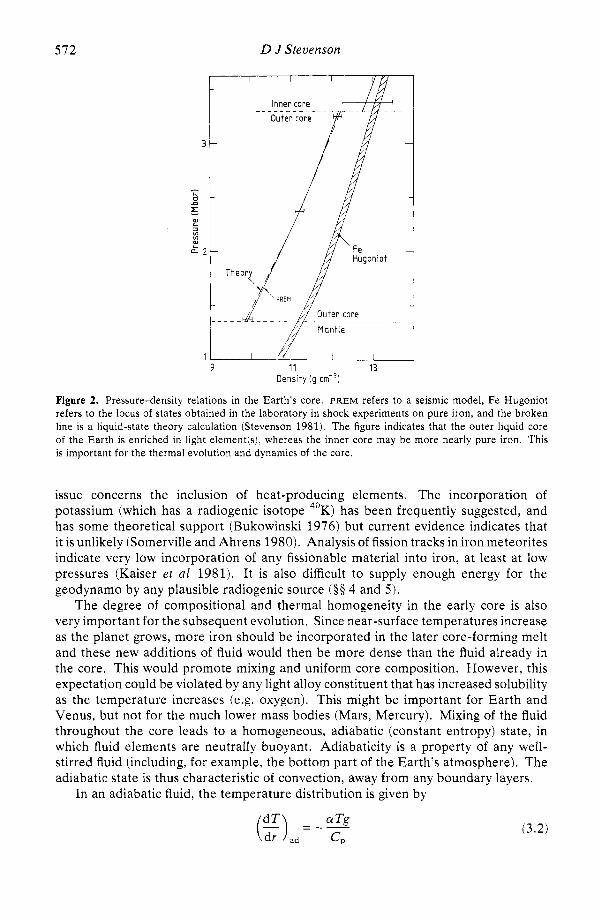
The composition of the core-forming fluid is important for understanding the subsequent evolution. In the Earth, the actual density of the outer core is 8 - l l% less than the density of pure iron at the same pressures and temperatures inferred from shockwave data (see figure 2). There are many possible candidate elements responsible for this density reduction, but the most likely ones are oxygen and sulphur (see Ringwood (1979) and Stevenson (1981) for reviews). Sulphur alloys with iron at low pressure and temperature and shockwave results for Feo$ and FeSz (Ahrens 1979, Ahrens and Creaven 1982) indicate that 8-12% of sulphur by mass is needed to explain the outer core density. This is about a factor of three less than cosmic abundance, but since sulphur is a volatile in the nebula out of which the planetesimals form, it is doubtful whether even one-third of the cosmic abundance was incorporated in the Earth. Oxygen probably does not encounter this problem, but has a different problem: it can only be incorporated into iron at high pressures, if at all. At low pressure ( P G 0.7 Mbar), oxygen is highly insoluble, but a transition of Fe0 to a more dense phase at 0.7Mbar (Jeanloz and Ahrens 1980) may favour incorporation of oxygen in the cores of Earth and Venus. This can only happen if the Fe-0 system has a greatly depressed melting point relative to pure iron, since incorporation in the core demands formation of a fluid (Stevenson 1981). McCammon eta1 (1982) describe a semiquantitative model for core formation in which oxygen is the major alloying constituent and a strongly depressed melting point occurs.
Of course, there is no need to assume that a single element is responsible for density reduction and melting point depression. Indeed, terrestrial planetary cores probably consist of as wide an assortment of elements as crustal rocks. One important
572 D J Stevenson
9 11 13 Density i g cm-7
Figure 2. Pressure-density relations in the Earth’s core. PREM refers to a seismic model, Fe Hugoniot refers to the locus of states obtained in the laboratory in shock experiments on pure iron, and the broken line is a liquid-state theory calculation (Stevenson 1981). The figure indicates that the outer liquid core of the Earth is enriched in light element(s), whereas the inner core may be more nearly pure iron. This is important for the thermal evolution and dynamics of the core.
issue concerns the inclusion of heat-producing elements. The incorporation of potassium (which has a radiogenic isotope 40K) has been frequently suggested, and has some theoretical support (Bukowinski 1976) but current evidence indicates that it is unlikely (Somerville and Ahrens 1980). Analysis of fission tracks in iron meteorites indicate very low incorporation of any fissionable material into iron, at least at low pressures (Kaiser er a1 1981). It is also difficult to supply enough energy for the geodynamo by any plausible radiogenic source (00 4 and 5 ) .
The degree of compositional and thermal homogeneity in the early core is also very important for the subsequent evolution. Since near-surface temperatures increase as the planet grows, more iron should be incorporated in the later core-forming melt and these new additions of fluid would then be more dense than the fluid already in the core. This would promote mixing and uniform core composition. However, this expectation could be violated by any light alloy constituent that has increased solubility as the temperature increases (e.g. oxygen). This might be important for Earth and Venus, but not for the much lower mass bodies (Mars, Mercury). Mixing of the fluid throughout the core leads to a homogeneous, adiabatic (constant entropy) state, in which fluid elements are neutrally buoyant. Adiabaticity is a property of any well- stirred fluid (including, for example, the bottom part of the Earth’s atmosphere). The adiabatic state is thus characteristic of convection, away from any boundary layers.
In an adiabatic fluid, the temperature distribution is given by
Planetary magnetic fields 573
or, equivalently,
where LY is the coefficient of thermal expansion, g is the gravitational acceleration, C, is the specific heat at constant pressure, y=aK,/pC, is the thermodynamic Griineisen parameter (dimensionless) and K, is the adiabatic bulk modulus (units of pressure). Typically, y - 1 and the adiabatic temperature gradient is a fraction of a degree per kilometre.
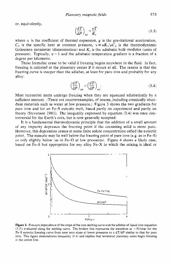
These formulae cease to be valid if freezing begins anywhere in the fluid. In fact, freezing is initiated at the planetary centre if it occurs at all. The reason is that the freezing curve is steeper than the adiabat, at least for pure iron and probably for any alloy:
Most terrestrial melts undergo freezing when they are squeezed adiabatically by a sufficient amount. (There are counterexamples, of course, including cosmically abun- dant materials such as water at low pressure.) Figure 3 shows the two gradients for pure iron and for an Fe-S eutectic melt, based partly on experiment and partly on theory (Stevenson 1981). The inequality expressed by equation (3.4) was once con- troversial for the Earth's core, but is now generally accepted.
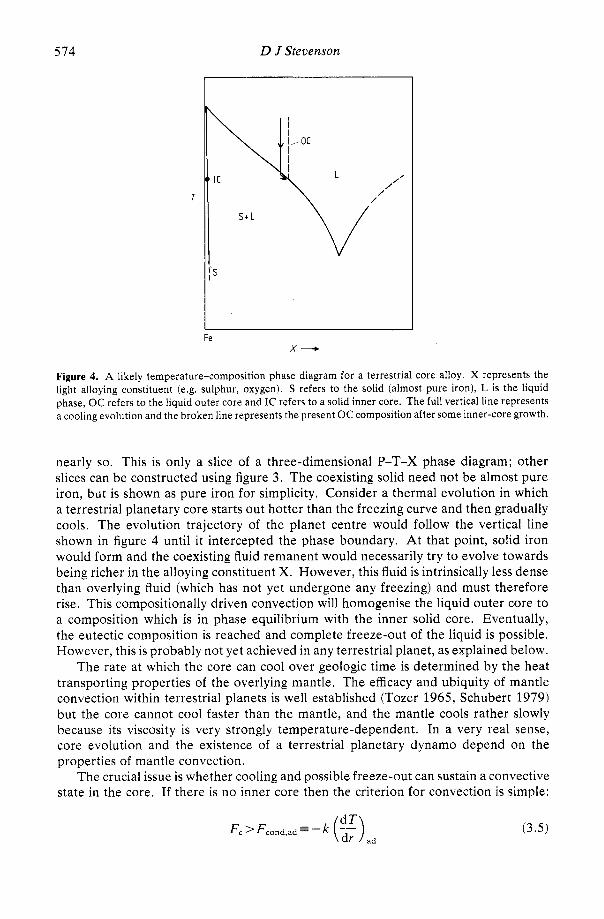
It is a fundamental thermodynamic principle that the addition of a small amount of any impurity depresses the freezing point if the coexisting solid is more pure. However, this depression ceases at some finite solute concentration called the eutectic point. The eutectic may lie well below the freezing point of pure iron (e.g. as in Fe-S) or only slightly below (as in Fe-0 at low pressures). Figure 4 shows a likely case, based on Fe-S but appropriate for any alloy Fe-X in which the mixing is ideal or
I ! \
0 2 4 PlMbar)
Figure 3. Pressure dependence of the slope of the iron melting curve and the adiabat of [iquid iron (equation (3.3)) evaluated along the melting curve. The broken line represents the transition at -50 kbar for the Fe-S eutectic freezing curve from near zero slope at lower pressures to a dT/dP similar to that for pure iron. This figure demonstrates inequality (3.4) and implies that terrestrial planetary cores begin freezing at the centre first.
574 D J Stevenson
I Fe
X +
Figure 4. A likely temperature-composition phase diagram for a terrestrial core alloy. X represents the light alloying constituent (e.g. sulphur, oxygen). S refers to the solid (almost pure iron), L is the liquid phase, OC refers to the liquid outer core and IC refers to a solid inner core. The full vertical line represents a cooling evolution and the broken line represents the present OC composition after some inner-core growth.
nearly so. This is only a slice of a three-dimensional P-T-X phase diagram; other slices can be constructed using figure 3. The coexisting solid need not be almost pure iron, bdt is shown as pure iron for simplicity. Consider a thermal evolution in which a terrestrial planetary core starts out hotter than the freezing curve and then gradually cools. The evolution trajectory of the planet centre would follow the vertical line shown in figure 4 until it intercepted the phase boundary, At that point, solid iron would form and the coexisting fluid remanent would necessarily try to evolve towards being richer in the alloying constituent X. However, this fluid is intrinsically less dense than overlying fluid (which has not yet undergone any freezing) and must therefore rise. This compositionally driven convection will homogenise the liquid outer core to a composition which is in phase equilibrium with the inner solid core. Eventually, the eutectic composition is reached and complete freeze-out of the liquid is possible. However, this is probably not yet achieved in any terrestrial planet, as explained below.
The rate at which the core can cool over geologic time is determined by the heat transporting properties of the overlying mantle. The efficacy and ubiquity of mantle convection within terrestrial planets is well established (Tozer 1965, Schubert 1979) but the core cannot cool faster than the mantle, and the mantle cools rather slowly because its viscosity is very strongly temperature-dependent. In a very real sense, core evolution and the existence of a terrestrial planetary dynamo depend on the properties of mantle convection.
The crucial issue is whether cooling and possible freeze-out can sustain a convective state in the core. If there is no inner core then the criterion for convection is simple:
Planetary magnetic fields 575
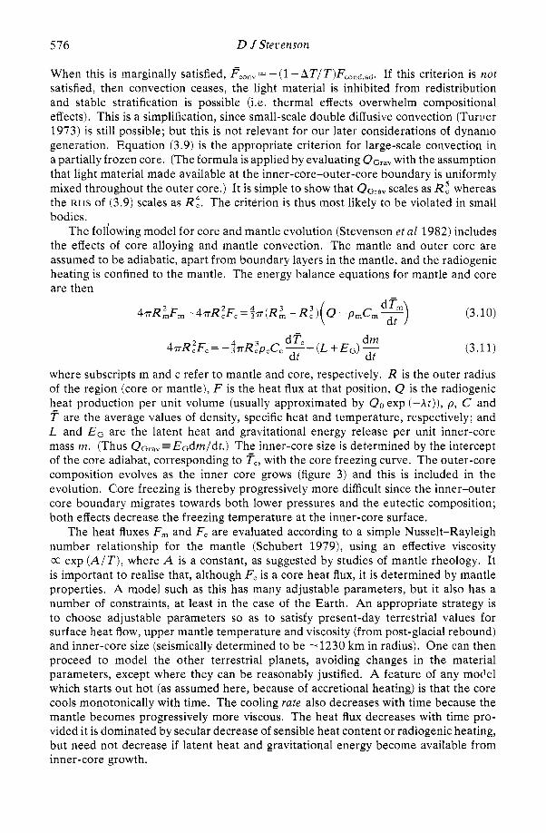
where F, is the actual core flux and Fcond,ad is the heat flux that can be transported by conduction along an adiabat (k is the outer-core thermal conductivity). If Fc< Fcond,ad, then the temperature profile is subadiabatic (and therefore stable to large-scale vertical motions) and given approximately by dT/dr = - FJk. If F, >Fcond,ad then the profile will be close to adiabatic (exactly how close is discussed in 8 4). The ‘excess’ heat flow (Fc -Fcond,ad) is then transported convectively. The following approximate calculation suggests that there might be no ‘excess’ (and hence no purely thermal convection) in present-day terrestrial cores. According to simple recipes describing subsolidus mantle convection (Schubert 1979), the heat flow transported by the mantle scales like AT4/3~-1/3, where AT is the temperature drop driving the convection and v is the mantle viscosity. The viscosity is so strongly dependent on temperature (v-T-‘, 2 0 ~ 7 7 ~ 3 0 over a small range of T) that the mantle temperature (and hence the core temperature, which is coupled to it) changes very slowly on a geologic time scale. For a planetary model which starts hot and then slowly cools as the radiogenic sources decay, the rate of decrease in core temperature is typically -200 K/109 yr (Stevenson et a1 1982). The resulting heat flux out of the core is given by multiplying this by core heat capacity and then dividing by the surface area: the result is -2(Rc/103 km) erg cmP2 s-l, where R, is the core radius. By comparison, Fcond,ad is about 3-5(RC/1O3 km) erg cm-* s-l using parameters given in Stevenson (1981). In this crude calculation, F ,<Fcond ,ad .
If an inner core is present then the upward mixing of a light constituent releases gravitational energy and convection can be sustained even when F, < Fcond,ad. To understand this, it is necessary to consider both the first and second laws of thermo- dynamics (Hewitt et a1 1975, Gubbins 1977a). Let Qth be the total energy release in the core from both intrinsic heat sources and secular release of heat (sensible and latent), let QGrav be the rate of gravitational energy release which goes into thermal energy (i.e. excluding work done against pressure) and, for completeness, let W be the rate at which work is done on the core by external processes (e.g. precessional torques, tides). The first law of thermodynamics states that
4 r R ZFc = Qth + QGrav -I- W. (3.6)
The second law states rigorously that the total dissipation (Ohmic, viscous, etc) Qtot
is bounded above:
(3.7)
where T,, Tu are the maximum and upper boundary temperatures in the core, respectively. However, Hewitt et a1 (1975) show that application of the Boussinesq approximation for a compositionally uniform core yields the approximate (but sufficiently accurate) result that
AT- @tot = --con, + QGrav + W
T m (3.8)
where AT = T, - Tu, and FconV is a radially averaged convective heat flux, which may be negative (i.e. positive compositional buoyancy may exceed negative thermal buoyancy in magnitude). In a case where QGrav dominates Qth or W, it follows from (3.6) and (3.8) that, since Otot > 0 if there is convection,
(3.9)
576 D J Stevenson
When this is marginally satisfied, Fconv= -(I -AT/T)F,ond,ad. If this criterion is not satisfied, then convection ceases, the light material is inhibited from redistribution and stable stratification is possible (i.e. thermal effects overwhelm compositional effects). This is a simplification, since small-scale double diffusive convection (Turiier 1973) is still possible; but this is not relevant for our later considerations of dynanio generation. Equation (3.9) is the appropriate criterion for large-scale convection in a partially frozen core. (The formula is applied by evaluating QGrav with the assumption that light material made available at the inner-core-outer-core boundary is uniformly mixed throughout the outer core.) It is simple to show that QGrav scales as RZ whereas the RHS of (3.9) scales as R:, The criterion is thus most likely to be violated in small bodies.
The foliowing model for core and mantle evolution (Stevenson et a1 1982) includes the effects of core alloying and mantle convection. The mantle and outer core are assumed to be adiabatic, apart from boundary layers in the mantle, and the radiogenic heating is confined to the mantle. The energy balance equations for mantle and core are then
dt ~ I T R ~ F , - ~ I T R : F , = $ I T ( R ~ - R:)( Q -pmCm
d Fc dm 4&F,= - & T R ~ ~ , C , - + ( L + E ~ ) - dt dt
(3.10)
(3.11)
where subscripts m and c refer to mantle and core, respectively. R is the outer radius of the region (core or mantle), F is the heat flux at that position, Q is the radiogenic heat production per unit volume (usually approximated by Qo exp ( - A t ) ) , p , C and F are the average values of density, specific heat and temperature, respectively; and L and EG are the latent heat and gravitational energy release per unit inner-core mass m. (Thus QGrav = EGdm/dt.) The inner-core size is determined by the intercept of the core adiabat, corresponding to Fc, with the core freezing curve. The outer-core composition evolves as the inner core grows (figure 3) and this is included in the evolution. Core freezing is thereby progressively more difficult since the inner-outer core boundary migrates towards both lower pressures and the eutectic composition; both effects decrease the freezing temperature at the inner-core surface.
The heat fluxes F, and F, are evaluated according to a simple Nusselt-Rayleigh number relationship for the mantle (Schubert 1979), using an effective viscosity CC exp (AIT) , where A is a constant, as suggested by studies of mantle rheology. It is important to realise that, although F, is a core heat flux, it is determined by mantle properties. A model such as this has many adjustable parameters, but it also has a number of constraints, at least in the case of the Earth. An appropriate strategy is to choose adjustable parameters so as to satisfy present-day terrestrial values for surface heat flow, upper mantle temperature and viscosity (from post-glacial rebound) and inner-core size (seismically determined to be -1230 km in radius). One can then proceed to model the other terrestrial planets, avoiding changes in the material parameters, except where they can be reasonably justified. A feature of any moclel which starts out hot (as assumed here, because of accretional heating) is that the core cools monotonically with time. The cooling rate also decreases with time because the mantle becomes progressively more viscous. The heat flux decreases with time pro- vided it is dominated by secular decrease of sensible heat content or radiogenic heating, but need not decrease if latent heat and gravitational energy become available from inner-core growth.
Planetary magnetic fields 5 77
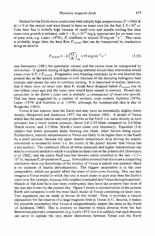
Models for the Earth were constructed with initially high temperatures ( T = 5000 K at t = 0 at the centre) and were found to have no inner core for the first 2-3 x lo9 yr. Core heat flux is initially high because of rapid core and mantle cooling but once inner-core growth is initiated, with L + EG = 10” erg/g (appropriate for an inner core of pure iron, e.g. Loper (1978)), F, stabilises at around 20 erg cm-’s-’. This value is probably larger than the heat flow Fcond,ad that can be transported by conduction along an adiabat
d T Fcond,ad = - k (z ) = 15 erg cm-2 s-1
ad (3.12)
(see Stevenson (1981) for parameter values) and the excess must be transported by convection. If upward mixing of light alloying material occurs then convection would ensue even if F, < Fcond,ad. Progressive core freezing continues up to and beyond the present day as the mantle continues to cool (because of the decaying radiogenic heat sources) and causes the core to continue cooling. It is important to realise, however, that if there were no inner core then F, would have dropped below F c o n d , a d one or two billion years ago and the outer core would have ceased to convect. Present-day convection in the Earth’s outer core is probably a consequence of inner-core growth. This has been suggested by a number of workers, most notably Gubbins (1976), Loper (1978) and Gubbins et a1 (1979); although the fundamental idea is due to Braginsky (1963).
Venus is less massive than the Earth and may have an intrinsically slightly lower density (Ringwood and Anderson 1977, but see Goettel 1982). A model of Venus which has the same mantle and core properties as the Earth (i.e. same density at each pressure) has a lower central pressure; about 2.8-2.95 Mbar compared to 3.6 Mbar (Earth centre) and 3.2 Mbar (Earth’s inner-outer core boundary). Equation (3.4) implies that lower pressures make freezing less likely, other factors being equal. Furthermore, internal temperatures in Venus are likely to be higher than in the Earth by a small amount, because the upper mantle temperature drop driving the mantle convection is necessarily lower (i.e. the centre of the planet ‘knows’ that Venus has a hot surface). The combined effects of lower pressures and higher temperatures can lead to evolution models in which Venus has no inner core at the present day (Stevenson et a1 1982), and the entire fluid core has become stably stratified in the last -1.5 x lo9 yr, because F, drops below Fcond,ad. It should be stressed that this is not a compelling conclusion since our knowledge of the interior of Venus is almost non-existent (there is no moment of inertia determination). The biggest uncertainty is in the core composition, which can greatly affect the onset of inner-core freezing. One can also imagine a Venus model in which the core is much closer to pure iron than the Earth’s outer core (for example, because little sulphur is included into Venus during formation). Models of this kind have also been constructed; they have the property that most of the core has frozen by the present day. Figure 5 shows a representation of the present Earth and compares it with the most likely model of Venus containing no inner core. Two arguments can be made in favour of this model. First, it provides a natural explanation for the absence of a large magnetic field in Venus (§ 5 ) . Second, it makes the plausible assumption that Venus is compositionally almost the same as the Earth (cf Anderson 1980). This is contrary to theories in which distance from the Sun determines planetary composition (e.g. Lewis 1972) but it is unlikely that such theories can serve to explain the very minor distinctions between Venus and the Earth
578 D J Stevenson
6371
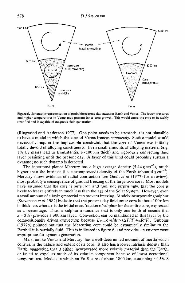
Earth Venus
Figure 5. Schematic representation of probable present-day states for Earth and Venus. The lower pressures and higher temperatures in Venus may prevent inner-core growth. This would cause the core to be stably stratified and incapable of magnetic-field generation.
(Ringwood and Anderson 1977). One point needs to be stressed: it is not plausible to have a model in which the core of Venus freezes completely. Such a model would necessarily require the implausible constraint that the core of Venus was initially totally devoid of alloying constituents. Even small amounts of alloying material (e.g. 1% by mass) lead to a substantial (-100 km thick) and vigorously convecting fluid layer persisting until the present day. A layer of this kind could probably sustain a dynamo; no such dynamo is detected.
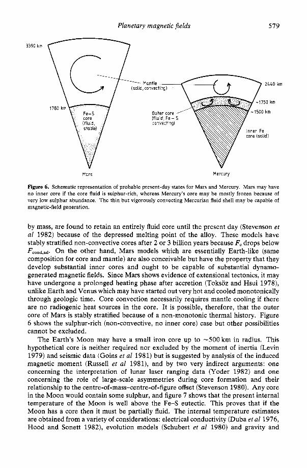
The innermost planet Mercury has a high average density (5.44 g ~ m - ~ ) , much higher than the intrinsic (i.e. uncompressed) density of the Earth (about 4 g cmP3). Mercury shows evidence of radial contraction (see Gault et a1 (1977) for a review), most probably a consequence of gradual freezing of the large iron core. Most models have assumed that the core is pure iron and find, not surprisingly, that the core is likely to freeze entirely in much less than the age of the Solar System. However, even a small amount of alloying material can prevent freezing. Models incorporating sulphur (Stevenson et a1 1982) indicate that the present-day fluid outer core is about 1OOx km in thickness where x is the initial mass fraction of sulphur for the entire core, expressed as a percentage. Thus, a sulphur abundance that is only one-tenth of cosmic (i.e. x = 3%) provides a 300 km layer. Convection can be maintained in this layer by the compositionally driven convection because Ec,,,dm/dt > (AT/T)4nR 'F,. Gubbins (1977b) pointed out that the Mercurian core could be dynamically similar to the Earth if it is partially fluid. This is indicated in figure 6 , and provides an environment appropriate for dynamo generation.
Mars, unlike Venus and Mercury, has a well-determined moment of inertia which constrains the nature and extent of its core. It also has a lower intrinsic density than Earth, suggesting that it either incorporated more volatile material than the Earth, or failed to expel as much of its volatile component because of lower accretional temperatures. Models in which an Fe-S core of about 1800 km, containing -15% S
Planetary magnetic fields 579
3390 km
1780 I”
km
Mars Mercury
Figure 6. Schematic representation of probable present-day states for Mars and Mercury. Mars may have no inner core if the core fluid is sulphur-rich, whereas Mercury’s core may be mostly frozen because of very low sulphur abundance. The thin but vigorously convecting Mercurian fluid shell may be capable of magnetic-field generation.
by mass, are found to retain an entirely fluid core until the present day (Stevenson et a1 1982) because of the depressed melting point of the alloy. These models have stably stratified non-convective cores after 2 or 3 billion years because F, drops below Fcond,ad. On the other hand, Mars models which are essentially Earth-like (same composition for core and mantle) are also conceivable but have the property that they develop substantial inner cores and ought to be capable of substantial dynamo- generated magnetic fields. Since Mars shows evidence of extensional tectonics, it may have undergone a prolonged heating phase after accretion (Toksoz and Hsui 1978), unlike Earth and Venus which may have started out very hot and cooled monotonically through geologic time. Core convection necessarily requires mantle cooling if there are no radiogenic heat sources in the core. It is possible, therefore, that the outer core of Mars is stably stratified because of a non-monotonic thermal history. Figure 6 shows the sulphur-rich (non-convective, no inner core) case but other possibilities cannot be excluded.
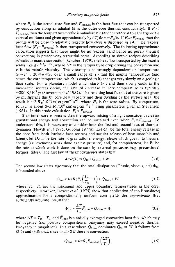
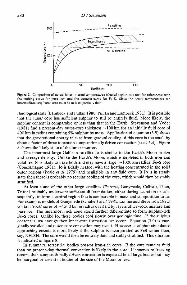
The Earth’s Moon may have a small iron core up to -500 km in radius. This hypothetical core is neither required nor excluded by the moment of inertia (Levin 1979) and seismic data (Goins et a1 1981) but is suggested by analysis of the induced magnetic moment (Russell et a1 1981), and by two very indirect arguments: one concerning the interpretation of lunar laser ranging data (Yoder 1982) and one concerning the role of large-scale asymmetries during core formation and their relationship to the centre-of-mass-centre-of-figure offset (Stevenson 1980). Any core in the Moon would contain some sulphur, and figure 7 shows that the present internal temperature of the Moon is well above the Fe-S eutectic. This proves that if the Moon has a core then it must be partially fluid. The internal temperature estimates are obtained from a variety of considerations: electrical conductivity (Duba et a1 1976, Hood and Sonett 1982), evolution models (Schubert et a1 1980) and gravity and
5 80 D J Stevenson
I - i\ --
7 Fe-S eutectic
I I I 0 500 1000 1500
D e p t h (km)
Figure 7. Comparison of actual lunar internal temperatures (shaded region, see text for references) with the melting curve for pure iron and the eutectic curve for Fe-S. Since the actual temperatures are intermediate, any lunar core must be at least partially fluid.
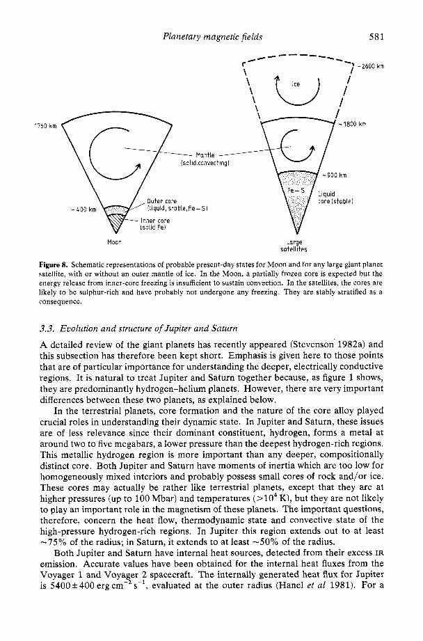
rheological state (Lambeck and Pullan 1980, Pullan and Lambeck 1981). It is possible that the lunar core has sufficient sulphur to still be entirely fluid. More likely, the sulphur content is comparable or less than that in the Earth. Stevenson and Yoder (1981) find a present-day outer-core thickness -100 km for an initially fluid core of 400 km in radius containing 5 % sulphur by mass. Application of equation (3.9) shows that the gravitational energy release from gradual cooling of this core is too small by about a factor of three to sustain compositionally driven convection (see § 5.4). Figure 8 shows the likely state of the lunar interior.
The innermost large Galilean satellite Io is similar to the Earth’s Moon in size and average density. Unlike the Earth’s Moon, which is depleted in both iron and volatiles, Io is likely to have both and may have a large (-1000 km radius) Fe-S core (Consolmagno 1981). Io is tidally heated, with the heating concentrated in the solid outer regions (Peale et al 1979) and negligible in any fluid core. If Io is in steady state then there is probably no secular cooling of the core, which would then be stably stratified.
At least some of the other large satellites (Europa, Ganymede, Callisto, Titan, Triton) probably underwent sufficient differentiation, either during accretion or sub- sequently, to form a central region that is comparable in mass and composition to Io. For example, models of Ganymede (Schubert et a1 1981, Lunine and Stevenson 1982) contain ‘rock’ cores of -1500 km in radius overlaid by layers of ice-rock mixture and pure ice. The innermost rock zone could further differentiate to form sulphur-rich Fe-S cores. Unlike Io, these bodies cool slowly over geologic time. If the sulphur content is low enough then inner-core formation can occur. Equation (3.9) is mar- ginally satisfied and outer-core convection may result. However, a sulphur abundance approching cosmic is more likely if the sulphur is incorporated as FeS rather than, say, NH4SH. The core would then be entirely fluid and stably stratified. This situation is indicated in figure 8.
In summary, terrestrial bodies possess iron-rich cores. If the core remains fluid then no present-day thermal convection is likely in the core. If inner-core freezing occurs, then compositionally driven convection is expected in all large bodies but may be marginal or absent in bodies of the size of the Moon or less.
Planetary magnetic fields 581
1760 k m
Moon iarge satellites
Figure 8. Schematic representations of probable present-day states for Moon and for any large giant planet satellite, with or without an outer mantle of ice. In the Moon, a partially frozen core is expected but the energy release from inner-core freezing is insufficient to sustain convection. In the satellites, the cores are likely to be sulphur-rich and have probably not undergone any freezing. They are stably stratified as a consequence.
3.3. Evolution and structure of Jupiter and Saturn
A detailed review of the giant planets has recently appeared (Stevenson 1982a) and this subsection has therefore been kept short. Emphasis is given here to those points that are of particular importance for understanding the deeper, electrically conductive regions. It is natural to treat Jupiter and Saturn together because, as figure 1 shows, they are predominantly hydrogen-helium planets. However, there are very important differences between these two planets, as explained below.
In the terrestrial planets, core formation and the nature of the core alloy played crucial roles in understanding their dynamic state. In Jupiter and Saturn, these issues are of less relevance since their dominant constituent, hydrogen, forms a metal at around two to five megabars, a lower pressure than the deepest hydrogen-rich regions. This metallic hydrogen region is more important than any deeper, compositionally distinct core. Both Jupiter and Saturn have moments of inertia which are too low for homogeneously mixed interiors and probably possess small cores of rock and/or ice. These cores may actually be rather like terrestrial planets, except that they are at higher pressures (up to 100 Mbar) and temperatures (> lo4 K), but they are not likely to play an important role in the magnetism of these planets. The important questions, therefore, concern the heat flow, thermodynamic state and convective state of the high-pressure hydrogen-rich regions. In Jupiter this region extends out to at least -75% of the radius; in Saturn, it extends to at least -50% of the radius.
Both Jupiter and Saturn have internal heat sources, detected from their excess IR
emission. Accurate values have been obtained for the internal heat fluxes from the Voyager 1 and Voyager 2 spacecraft. The internally generated heat flux for Jupiter is 5400*400 erg cm-’s-’, evaluated at the outer radius (Hanel et a1 1981). For a
582 D J Stevenson
deep-seated energy source, this heat flux will scale as r-', where r is the distance from the centre. The corresponding flux for Saturn is 2000& 140 erg cm-'s-' (Hanel et a1 1982). For comparison, the internal heat flux at the Earth's surface is about 70 erg cm-'s-'. At regions deeper than about 0.5 bar in the atmosphere, the Jovian and Saturnian heat flows are too high to be transported by radiation or conduction along a subadiabatic temperature gradient (Stevenson and Salpeter 1977). Metallic hydrogen is a good thermal conductor with k - 1 to 2 x 10' erg cm-' s-' K-' but with an adiabatic gradient of about -0.2Kkm-', the conductive heat flow is only 400 erg cm-'s-' at most; comfortably less than the actual heat flow.
An adiabatic, convective state therefore prevails and the temperature rises with pressure:
T = TIP" (3.13)
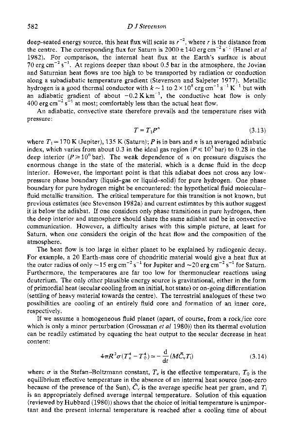
where T1 = 170 K (Jupiter), 135 K (Saturn); P is in bars and n is an averaged adiabatic index, which varies from about 0.3 in the ideal gas region (P s lo3 bar) to 0.28 in the deep interior ( P a lo6 bar). The weak dependence of n on pressure disguises the enormous change in the state of the material, which is a dense fluid in the deep interior. However, the important point is that this adiabat does not cross any low- pressure phase boundary (liquid-gas or liquid-solid) for pure hydrogen. One phase boundary for pure hydrogen might be encountered: the hypothetical fluid molecular- fluid metallic transition. The critical temperature for this transition is not known, but previous estimates (see Stevenson 1982a) and current estimates by this author suggest it is below the adiabat. If one considers only phase transitions in pure hydrogen, then the deep interior and atmosphere should share the same adiabat and be in convective communication. However, a difficulty arises with this simple picture, at least for Saturn, when one considers the origin of the heat flow and the composition of the atmosphere.
The heat flow is too large in either planet to be explained by radiogenic decay. For example, a 20 Earth-mass core of chondritic material would give a heat flux at the outer radius of only -15 erg cm-'s-' for Jupiter and -20 erg cm-* s-' for Saturn. Furthermore, the temperatures are far too low for thermonuclear reactions using deuterium. The only other plausible energy source is gravitational, either in the form of primordial heat (secular cooling from an initial, hot state) or on-going differentiation (settling of heavy material towards the centre). The terrestrial analogues of these two possibilities are cooling of an entirely fluid core and formation of an inner core, respectively.
If we assume a homogeneous fluid planet (apart, of course, from a rock/ice core which is only a minor perturbation (Grossman et a1 1980)) then its thermal evolution can be readily estimated by equating the heat output to the secular decrease in heat content:
d dt
47tR2u(T2 - T!) 2: - - (McvTj) (3.14)
where U is the Stefan-Boltzmann constant, T, is the effective temperature, To is the equilibrium effective temperature in the absence of an internal heat source (non-zero because of the presence of the Sun), cv is the average specific heat per gram, and Ti is an appropriately defined average internal temperature. Solution of this equation (reviewed by Hubbard (1980)) shows that the choice of initial temperature is unimpor- tant and the present internal temperature is reached after a cooling time of about
Planetary magnetic Felds 583
5 x lo9 yr for Jupiter and 2.5-3.5 x lo9 yr for Saturn (the latter corrected for the new, lower estimate of Saturn's heat flow (Hanel et a1 1982)). The result for Jupiter is consistent, within uncertainties, with the age of the Solar System ( ~ 4 . 6 x lo9 yr). The result for Saturn is probably not; the shortfall indicates the need for an additional energy source (unless one is willing to contemplate the unorthodox hypothesis that Saturn formed more recently than Jupiter). The explanation appears to be that Saturn, because it is colder, is undergoing phase separation of helium from hydrogen. Helium is predicted to have limited solubility in metallic hydrogen (see Stevenson (1982a) for a complete discussion of this). The downward displacement of helium as raindrops releases additional energy. This hypothesis is supported by the low helium abundance in the Saturnian atmosphere (-10% by mass) compared to that in Jupiter's atmosphere (-20% by mass). The consequence of this phase separation is a Saturnian internal structure consisting of a helium-depleted envelope, an intermediate conditionally stable layer in which there is a helium gradient, and a helium-enriched core. Both the envelope and the core undergo large-scale convection, but there is no longer direct convective communication between these regions. Figure 9 shows models for Jupiter and Saturn implied by these considerations. The qualitative differences in their internal structures may explain the differences in their magnetic fields (§ 5 ) .
69800 k m
- 55000
/ H,-Hefluid \
/------ 7 58400
H,-He fluid (convecting, ' I insulator1
29000 k m
24000 km!
Stable metallic f i u id
metaliic f l u id (convecting)
-15000 km Rock ( + ice? 1
core
km
Jupiter Saturn
Figure 9. Schematic representation of probable present-day states for Jupiter and Saturn. Except for an intermediate, metallic fluid layer in Saturn, which is stably stratified because of a helium gradient, these planets are expected to be vigorously convective throughout.
3.4. Evolution and structure of Uranus and Neptune
The internal structures of these planets have been recently reviewed (Stevenson 1982a), but see also Podolak (1982) and Hubbard and MacFarlane (1982). As figure 1 shows, the compositions of Uranus and Neptune are not obvious from their average densities. Ices (HzO, NH3 and CH4) must be a major component but these planets possess hydrogen-rich atmospheres and moments of inertia which point to a three-layer

584 D J Stevenson
structure: a rock core, an ice mantle and a deep, light atmosphere. The moment of inertia for Uranus is now quite well established, albeit indirectly (from an analysis of precession of some of its rings and measurement of the planetary oblateness). The type of model most consistent with these data has an outer gas layer enriched in material heavier than hydrogen or helium; plausibly methane and/or water. The upper level of the ice layer is about 200 kbar pressure, and the interface between ice and rock is typically at around 5 Mbar, possibly significant in view of our earlier discussion of pressure metallisation at a few megabars.
An internal heat flow has been detected for Neptune and corresponds to -250 erg cm-'s-' in the deep atmosphere. Only an upper bound (-180 erg cm-2 sC1) exists for Uranus, but the similarity of this bound to the measured Neptunian heat flow means that it would be premature to argue that Uranus is significantly different in behaviour. Hubbard (1980j pointed out that a Uranian heat flow may be both harder to detect and reduced slightly because of the planet's closer distance to the Sun. Heat flows of -lo2 erg cm-2 s-' could be provided by gradual cooling from a primordial hotter state, as with Jupiter, although this primordial state could not have been as much as twice the internal temperature of the present state (Hubbard and MacFarlane 1980). The important issue for our considerations, however, is whether this heat flow requires an adiabatic, convective state.
If the outer regions are adiabatic then the ice layer is well above its freezing point. In the dense, molecular or ionic fluid comprising the ice layer, the thermal conductivity k is likely to be about 106ergcm-' s-'K-'. This estimate is obtained from the equation k = pC&, where p = 2 g ~ m - ~ , C, = 5 x lo7 erg g-' and K = lop2 cm2 s-' (typical of molecular fluids). The Griineisen y (equation (3.3)) is likely to be in the range 0.5-1 (Mitchell and Nellis 1982) and an adiabatic temperature gradient of 0.5-1 K km-' is implied. The conductive heat flow is about 10 erg cm-2 s-l, comfort- ably less than the actual heat flow. If the ice layer is metallic in its deepest regions, then the conductivity would increase by about one order of magnitude, perhaps even more, and it is no longer clear whether thermal convection would persist.
The rock core, of about two Earth masses, is likely to differentiate into an iron-rich fluid central region and a silicate-rich, partially solid region (Torbett and Smoluchowski 1980). They pointed out that the hypothesised limited solubility of MgO in an Fe-S-0 fluid might cause phase separation and the release of gravitational energy, sufficient to maintain convection and a dynamo. This may happen, but it is straightforward to show that secular cooling alone of the innermost region would yield a local heat flow of around 100 erg cm-* s-', more than sufficient to maintain thermal convection.
Figure 10 shows a schematic model of Uranus or Neptune, indicating thermal convection everywhere except possibly in the lowermost ice region, if that region is metallic. As discussed in 8 5 , this structure is likely to sustain a magnetic field, although the dominant source region is not clearly identified.
4. The sources of planetary magnetism
4.1. Non-dynamo sources
As mentioned in the introduction, Ohm's law predicts the decay of macroscopic currents in a geologically short time, if there are no induction effects as in a dynamo. However, there are many ways of producing electrical currents and associated mag- netic fields which do not satisfy Ohm's law. Most of the alternatives are catalogued
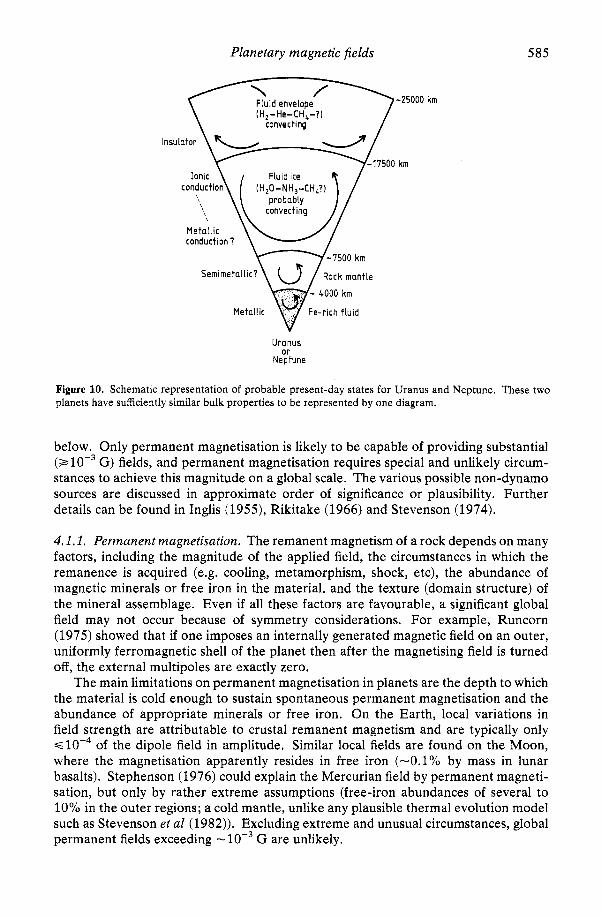
Planetary magnetic fields 585
Fluid envelope (H,-He-CH,-?I
convecting
Insulator k = = 5 0 0 km
Uranus or
Neotune
Figure 10. Schematic representation of probable present-day states for Uranus and Neptune. These two planets have sufficieitly similar bulk properties to be represented by one diagram.
below. Only permanent magnetisation is likely to be capable of providing substantial (B lop3 G) fields, and permanent magnetisation requires special and unlikely circum- stances to achieve this magnitude on a global scale. The various possible non-dynamo sources are discussed in approximate order of significance or plausibility. Further details can be found in Inglis (1955), Rikitake (1966) and Stevenson (1974).
4.1.1. Permanent magnetisation. The remanent magnetism of a rock depends on many factors, including the magnitude of the applied field, the circumstances in which the remanence is acquired (e.g. cooling, metamorphism, shock, etc), the abundance of magnetic minerals or free iron in the material, and the texture (domain structure) of the mineral assemblage. Even if all these factors are favourable, a significant global field may not occur because of symmetry considerations. For example, Runcorn (1975) showed that if one imposes an internally generated magnetic field on an outer, uniformly ferromagnetic shell of the planet then after the magnetising field is turned off, the external multipoles are exactly zero.
The main limitations on permanent magnetisation in planets are the depth to which the material is cold enough to sustain spontaneous permanent magnetisation and the abundance of appropriate minerals or free iron. On the Earth, local variations in field strength are attributable to crustal remanent magnetism and are typically only <lop4 of the dipole field in amplitude. Similar local fields are found on the Moon, where the magnetisation apparently resides in free iron (-0.1% by mass in lunar basalts). Stephenson (1976) could explain the Mercurian field by permanent magneti- sation, but only by rather extreme assumptions (free-iron abundances of several to 10% in the outer regions; a cold mantle, unlike any plausible thermal evolution model such as Stevenson et a1 (1982)). Excluding extreme and unusual circumstances, global permanent fields exceeding G are unlikely.
D J Stevenson
4.1.2. External induction. Repeated magnetic storms or variability in solar magnetic fields can induce current systems in planetary interiors. Significant fields could accumu- late if the effects had a net sense of induction, but the fluctuating nature of inducing fields prevents a significant cumulative effect, despite the relatively long free decay time of the induced currents (Price 1962).
4.1.3. Thermoelectric effects (Elsasser 1939). Temperature gradients in the presence of electrical conductors of different compositions (i.e. different chemical potentials) cause persistent electrical currents. Realistic estimates of likely temperature differ- ences and thermopowers lead to very small fields in planets ( d o v 3 G, typically, e.g. Merrill et a1 1979). The field produced is toroidal and one could imagine, in principle, a planetary core in which a small thermoelectric toroidal field is the seed for the amplification of a large poloidal field by vertical fluid motions. This is not a dynamo, but involves ‘half’ of a dynamo.
4.1.4. Thermomagnetic effects (Nernst-Ettinghausen effect). In the presence of a radial temperature gradient and an axial magnetic field, electric currents are created which can augment the initial field. This process fails to be regenerative for the Earth by a factor of several thousands, for any plausible combination of the relevant material parameters (Stevenson 1974). Curiously, this process has received a revival of interest (Hibberd 1979) and was subsequently shown to be deficient on more rigorous symmetry grounds (Hide 1979, Ivers and James 1981, Hide and Palmer 1982) unless one postulates unreasonable deviations from spherical symmetry.
4.1.5. Hall effect. This was suggested by Vestine (1954) for the Earth. Hall currents arise in a conductor if there are pre-existing currents and a magnetic field. The problem is that the Hall effect is much too small and inefficient for fields less than many kilogauss. It is, in effect, a second-order process that feeds on some other source (such as thermoelectric currents) which is already likely to be too small to be significant.
4.1.6. Compression effect. Electrons and ions respond differently to a gravity field and the result is a radial electric field within any self-gravitating body. However, this effect provides no prospect of a regenerative magnetic field because it provides no energy source (Stevenson 1974).
4.1.7. Rotating electric charge. Since the rotational velocity of a planet is much less than the speed of light, enormous electric charge densities and fields are required to produce significant magnetic fields. Typical required electric fields are - lo6 V m-*. There is no known way of creating and sustaining this field within a planet, especially since the ‘insulating’ regions of planets are very imperfect insulators.
4.1.8. Gyromagnetic effect. A rotating, ferromagnetic body is magnetised in the direction of the rotation axis by the effect of the macroscopic rotation on the micro- scopic electron currents. Only lo-’’ of the Earth’s field can be attributed to this (Rikitake 1966) and similar fractions apply to other planets.
4.1.9. Differential rotation. Very rapid differential rotation in a metallic fluid produces a net electron current which is proportional to the amount by which the fluid rotation changes over a distance of one electronic mean free path. This mechanism fails by over twelve orders of magnitude for the Earth (Inglis 1955).
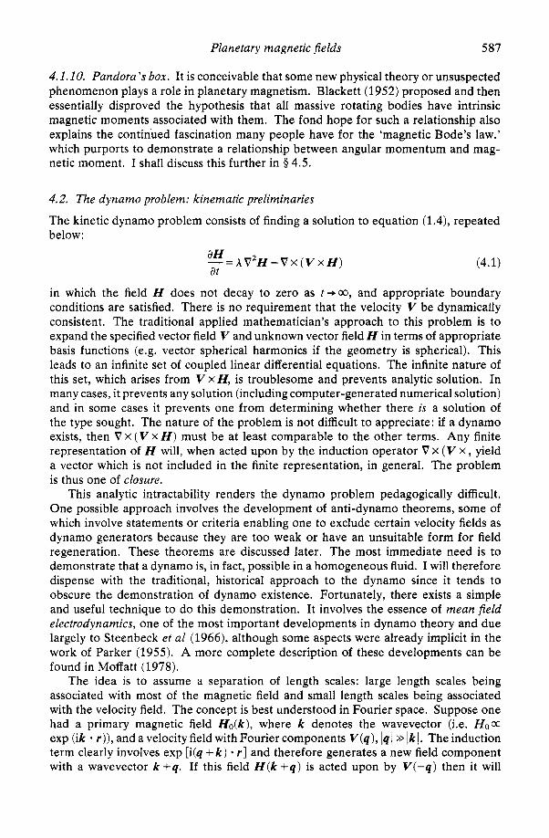
Planetary magnetic fields 587
4.1.10. Pandora’s box. It is conceivable that some new physical theory or unsuspected phenomenon plays a role in planetary magnetism. Blackett (1952) proposed and then essentially disproved the hypothesis that all massive rotating bodies have intrinsic magnetic moments associated with them. The fond hope for such a relationship also explains the continued fascination many people have for the ‘magnetic Bode’s law.’ which purports to demonstrate a relationship between angular momentum and mag- netic moment. I shall discuss this further in § 4.5.
4.2. The dynamo problem: kinematic preliminaries
The kinetic dynamo problem consists of finding a solution to equation (1,4), repeated below:
in which the field H does not decay to zero as t+m, and appropriate boundary conditions are satisfied. There is no requirement that the velocity V be dynamically consistent. The traditional applied mathematician’s approach to this problem is to expand the specified vector field V and unknown vector field H in terms of appropriate basis functions (e.g. vector spherical harmonics if the geometry is spherical). This leads to an infinite set of coupled linear differential equations. The infinite nature of this set, which arises from V x H, is troublesome and prevents analytic solution. In many cases, it prevents any solution (including computer-generated numerical solution) and in some cases it prevents one from determining whether there is a solution of the type sought. The nature of the problem is not difficult to appreciate: if a dynamo exists, then V x ( V x H ) must be at least comparable to the other terms. Any finite representation of H will, when acted upon by the induction operator V x (V x , yield a vector which is not included in the finite representation, in general. The problem is thus one of closure.
This analytic intractability renders the dynamo problem pedagogically difficult. One possible approach involves the development of anti-dynamo theorems, some of which involve statements or criteria enabling one to exclude certain velocity fields as dynamo generators because they are too weak or have an unsuitable form for field regeneration. These theorems are discussed later. The most immediate need is to demonstrate that a dynamo is, in fact, possible in a homogeneous fluid. I will therefore dispense with the traditional, historical approach to the dynamo since it tends to obscure the demonstration of dynamo existence. Fortunately, there exists a simple and useful technique to do this demonstration. It involves the essence of mean field electrodynamics, one of the most important developments in dynamo theory and due largely to Steenbeck et a1 (1966), although some aspects were already implicit in the work of Parker (1955). A more complete description of these developments can be found in Moffatt (1978).
The idea is to assume a separation of length scales: large length scales being associated with most of the magnetic field and small length scales being associated with the velocity field. The concept is best understood in Fourier space. Suppose one had a primary magnetic field H&), where k denotes the wavevector (i.e. Hoot exp (ik a r ) ) , and a velocity field with Fourier components V ( q ) , 141 >> Ik I. The induction term clearly involves exp [i(q + k) - r ] and therefore generates a new field component with a wavevector k + q . If this field H ( k + q ) is acted upon by V ( - q ) then it will
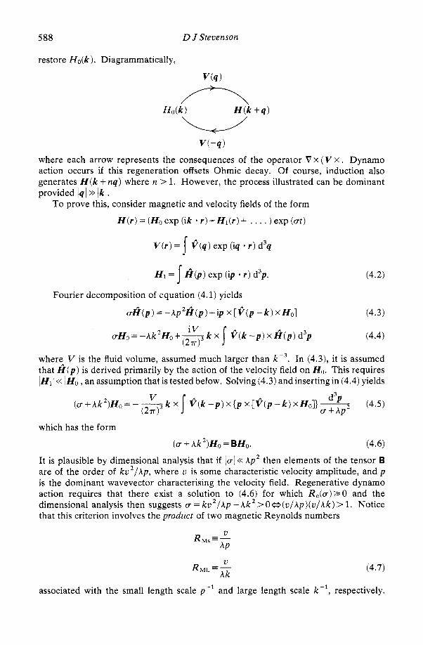
588 D J Stevenson
restore Ho(k) . Diagrammatically,
V ( - 4 )
where each arrow represents the consequences of the operator V x (V x . Dynamo action occurs if this regeneration offsets Ohmic decay. Of course, induction also generates H ( k + n q ) where n > 1. However, the process illustrated can be dominant provided 141 >> lkl.
To prove this, consider magnetic and velocity fields of the form
H ( r ) = (Ho exp (ik r ) + H l ( r ) + . . . . ) exp (at)
V ( r ) = Q ( q ) exp (iq r ) d3q
H I = fib) exp (ip r ) d3p. (4.2) J Fourier decomposition of equation (4.1) yields
&(p ) = -Ap 'fi ( p ) + ip x [ o ( p - k ) X Ho] (4.3)
(4.4) aHO=-Ak ~ ~ + y k x J f ( k - p ) x f i ( p ) d 3 p
where V is the fluid volume, assumed much larger than k - 3 . In (4.3), it is assumed that fi(p) is derived primarily by the action of the velocity field on MO. This requires lH1/ << /HO/ , an assumption that is tested below. Solving (4.3) and insertingin (4.4) yields
2 i V (27 )
which has the form
(v +Ak')Ho = BH,. (4.6)
It is plausible by dimensional analysis that if lul<< Ap2 then elements of the tensor B are of the order of kv2/Ap, where v is some characteristic velocity amplitudc, and p is the dominant wavevector characterising the velocity field. Regenerative dynamo action requires that there exist a solution to (4.6) for which R,(a)>O and the dimensional analysis then suggests v = kv2/Ap - A k 2 > O(J(u/Ap)(v/Ak)> 1. Notice that this criterion involves the product of two magnetic Reynolds numbers
U R =_ Ms - Ap
U R M L " -
Ak (4.7)
associated with the small length scale p - l and large length scale k - ' , respectively.
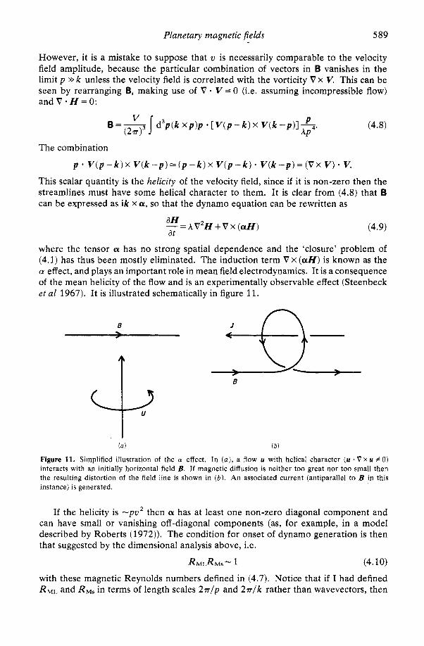
Planetary magnetic fields 589
However, it is a mistake to suppose that U is necessarily comparable to the velocity field amplitude, because the particular combination of vectors in B vanishes in the limit p >> k unless the velocity field is correlated with the vorticity V x V. This can be seen by rearranging B, making use of V . V = O (i.e. assuming incompressible flow) and V * H = 0:
(4.8)
The combination
p * V ( p - k ) x V ( k - - p ) - ( p - k ) x V ( p - k ) . V ( k - p ) = ( V x V ) * v. This scalar quantity is the helicity of the velocity field, since if it is non-zero then the streamlines must have some helical character to them. It is clear from (4.8) that B can be expressed as ik x a, so that the dynamo equation can be rewritten as
dH at - = AV’H + v x ( a ~ ) (4.9)
where the tensor a has no strong spatial dependence and the ‘closure’ problem of (4.1) has thus been mostly eliminated. The induction term V X ( a H ) is known as the a effect, and plays an important role in mean field electrodynamics. It is a consequence of the mean helicity of the flow and is an experimentally observable effect (Steenbeck et a1 1967). It is illustrated schematically in figure 11.
B
t B
((1 ) (bl
Figure 11. Simplified illustration of the a effect. In ( a ) , a flow U with helical character (U . V X U #0) interacts with an initially horizontal field B. If magnetic diffusion is neither too great nor too small then the resulting distortion of the field line is shown in (b ) . An associated current (antiparallel to B in this instance) is generated.
If the helicity is -pu’ then a has at least one non-zero diagonal component and can have small or vanishing off-diagonal components (as, for example, in a model described by Roberts (1972)). The condition for onset of dynamo generation is then that suggested by the dimensional analysis above, i.e.
RMLRMS- 1 (4.10)
with these magnetic Reynolds numbers defined in (4.7). Notice that if I had defined RML and R M s in terms of length scales 2 v / p and 2 r / k rather than wavevectors, then
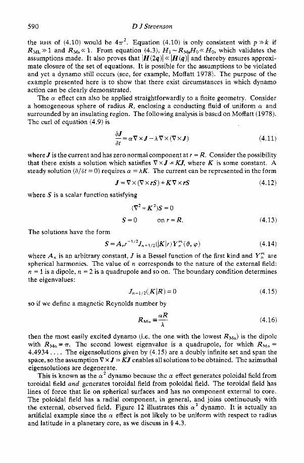
590 D J Stevenson
the RHS of (4.10) would be 4r2. Equation (4.10) is only consistent with p >> k if RML >> 1 and R M ~ << 1. From equation (4.3), HI - R M ~ H O << Ho, which validates the assumptions made. It also proves that IH(2q)I << IIP (q)1 and thereby ensures approxi- mate closure of the set of equations. It is possible for the assumptions to be violated and yet a dynamo still occurs (see, for example, Moffatt 1978). The purpose of the example presented here is to show that there exist circumstances in which dynamo action can be clearly demonstrated.
The a effect can also be applied straightforwardly to a finite geometry. Consider a homogeneous sphere of radius R , enclosing a conducting fluid of uniform a and surrounded by an insulating region. The following analysis is based on Moffatt (1978). The curl of equation (4.9) is
(4.11)
where J is the current and has zero normal component at r = R . Consider the possibility that there exists a solution which satisfies V x J = KJ, where K is some constant. A steady solution ( a l a r = 0) requires a = AK. The current can be represented in the form
J = V x (V x rS) +KV xrS (4.12)
a J at -=aV X J - A V X (v X J )
where S is a scalar function satisfying
(V2 +K2)S = 0
s=o o n r = R .
The solutions have the form
S =A,r-1’2J,+1,2(lKlr)Yr (6, c p )
(4.13)
(4.14)
where A , is an arbitrary constant, J is a Bessel function of the first kind and Y r are spherical harmonics. The value of n corresponds to the nature of the external field: n = 1 is a dipole, n = 2 is a quadrupole and so on. The boundary condition determines the eigenvalues:
Jn+l,2(lKlR) = 0 (4.15)
so if we define a magnetic Reynolds number by
aR RMa E -
A (4.16)
then the most easily excited dynamo (i.e. the one with the lowest RMa) is the dipole with RMa= T. The second lowest eigenvalue is a quadrupole, for which RMa = 4.4934. . . . The eigensolutions given by (4.15) are a doubly infinite set and span the space, so the assumption V x J = KJ enables all solutions to be obtained. The azimuthal eigensolutions are degenerate.
This is known as the a’ dynamo because the a effect generates poloidal field from toroidal field and generates toroidal field from poloidal field. The toroidal field has lines of force that lie on spherical surfaces and has no component external to core. The poloidal field has a radial component, in general, and joins continuously with the external, observed field. Figure 12 illustrates this a2 dynamo. It is actually an artificial example since the a effect is not likely to be uniform with respect to radius and latitude in a planetary core, as we discuss in § 4.3.
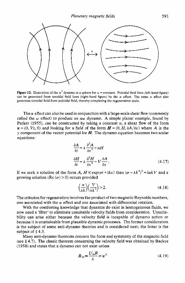
Planetary magnetic fields 591
Figure 12. Illustration of the a2 dynamo in a sphere for a =constant. Poloidal field lines (left-hand figure) can be generated from toroidal field lines (right-hand figure) by the a effect. The same a effect also generates toroidal field from poloidal field, thereby completing the regeneration cycle.
The a effect can also be used in conjunction with a large-scale shear flow (commonly called the w effect) to produce an aw dynamo. A simple planar example, found by Parker (1955), can be constructed by taking a constant a, a shear flow of the form U = (0, Vz, 0) and looking for a field of the form H = (0, H, aA/ax) where A is the y component of the vector potential for H. The dynamo equation becomes two scalar equations:
aA a2A at ax -= A 7 + a H
aH a2H aA at ax ax -= A y + V - (4.17)
If we seek a solution of the form A, Hocexp(d + i k x ) then (a+Ak2)’ = i a k V and a growing solution (Re ((T) > 0) occurs provided
(E)(+ Ak Ak2 (4.18)
The criterion for regeneration involves the product of two magnetic Reynolds numbers, one associated with the a effect and one associated with differential rotation.
With the comforting knowledge that dynamos do exist in homogeneous fluids, we now need a ‘filter’ to eliminate unsuitable velocity fields from consideration. Unsuita- bility can arise either because the velocity field is incapable of dynamo action or because it is unattainable from plausible dynamic processes. The former consideration is the subject of some anti-dynamo theories and is considered next; the latter is the subject of 0 4.3.
Many anti-dynamo theorems concern the form and symmetry of the magnetic field (see 0 4.7). The classic theorem concerning the velocity field was obtained by Backus (1958) and states that a dynamo can not exist unless
(4.19)
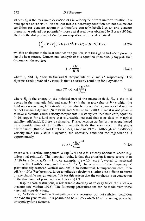
592 D J Stevenson
where U, is the maximum deviation of the velocity field from uniform rotation in a fluid sphere of radius R . Notice that this is a necessary condition but not a sufficient condition for dynamo action; it is therefore correctly labelled as an anti-dynamo theorem. A related but potentially more useful result was obtained by Busse (1975a). He took the dot product of the dynamo equation with r and obtained
which is analogous to the heat conduction equation, with the right-hand side represent- ing the heat source. Dimensional analysis of this equation immediately suggests that dynamo actidn requires
(4.21)
where v, and H, refers to the radial components of V and H, respectively. The rigorous result obtained by Busse is that a necessary condition for a dynamo is
(4.22)
where E, is the energy in the poloidal part of the magnetic field, EM is the total energy in the magnetic field and max ( V * r ) is the largest value of V r within the fluid region assuming V is steady. (It can also be shown that a purely radial motion cannot sustain a dynamo (Namikawa and Matsushita 1970).) Since it is not possible to have substantial radial velocity components in a stably stratified fluid core, equation (4.20) argues for a fluid core that is unstable (superadiabatic) or close to marginal stability (adiabatic), if there is a dynamo. This conclusion can be further strengthened by a consideration of the oscillatory velocity fields that may occur in the stable environment (Bullard and Gubbins 197 1, Gubbins 1975). Although an oscillatory velocity field can sustain a dynamo, the necessary condition for regeneration is approximately
1/2
uv b Aw( 2) (4.23)
where U is a vertical component Xexp (iwt) and v is a steady horizontal shear (e.g. differential rotation). The important point is that this criterion is more severe than (4.19) by a factor wR/v >> 1. (For example, if v - cms-l, typical of westward drift in the Earth’s core, and if w - s-I, characteristic of the frequency of gravitationally restored vertical motions in an isothermal, homogeneous core, then wR/v - lo6.) Furthermore, large-amplitude velocity oscillations are difficult to excite by any plausible energy source. It is for this reason that the emphasis is on convection in the discussion of planetary core flows in § 4.3.
Despite these restrictions, a remarkable diversity of velocity fields can sustain a dynamo (see Moffatt 1978). The following generalisations can be made from these kinematic considerations.
(i) Velocities of sufficient magnitude are a necessary but not sufficient condition for dynamo generation. It is possible to have flows which have the wrong geometry or topology for a dynamo.
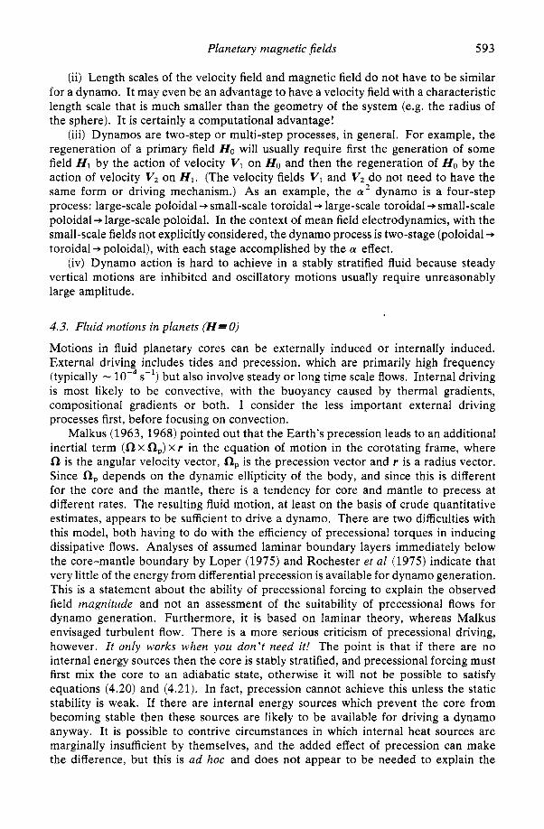
Planetary magnetic fields 593
(ii) Length scales of the velocity field and magnetic field do not have to be similar for a dynamo. It may even be an advantage to have a velocity field with a characteristic length scale that is much smaller than the geometry of the system (e.g. the radius of the sphere). It is certainly a computational advantage!
(iii) Dynamos are two-step or multi-step processes, in general. For example, the regeneration of a primary field Ho will usually require first the generation of some field H I by the action of velocity VI on Ho and then the regeneration of Ho by the action of velocity Vz on H 1 . (The velocity fields V1 and Vz do not need to have the same form or driving mechanism.) As an example, the a* dynamo is a four-step process: large-scale poloidal + small-scale toroidal + large-scale toroidal + small-scale poloidal+ large-scale poloidal. In the context of mean field electrodynamics, with the small-scale fields not explicitly considered, the dynamo process is two-stage (poloidal + toroidal + poloidal), with each stage accomplished by the a effect.
(iv) Dynamo action is hard to achieve in a stably stratified fluid because steady vertical motions are inhibited and oscillatory motions usually require unreasonably large amplitude.
4.3. Fluid motions in planets (H=O) Motions in fluid planetary cores can be externally induced or internally induced. External driving includes tides and precession, which are primarily high frequency (typically - s-l) but also involve steady or long time scale flows. Internal driving is most likely to be convective, with the buoyancy caused by thermal gradients, compositional gradients or both. I consider the less important external driving processes first, before focusing on convection.
Malkus (1963, 1968) pointed out that the Earth’s precession leads to an additional inertial term (fl X flp) x r in the equation of motion in the corotating frame, where fl is the angular velocity vector, np is the precession vector and r is a radius vector. Since aP depends on the dynamic ellipticity of the body, and since this is different for the core and the mantle, there is a tendency for core and mantle to precess at different rates. The resulting fluid motion, at least on the basis of crude quantitative estimates, appears to be sufficient to drive a dynamo. There are two difficulties with this model, both having to do with the efficiency of precessional torques in inducing dissipative flows. Analyses of assumed laminar boundary layers immediately below the core-mantle boundary by Loper (1975) and Rochester et a1 (1975) indicate that very little of the energy from differential precession is available for dynamo generation. This is a statement about the ability of precessional forcing to explain the observed field magnitude and not an assessment of the suitability of precessional flows for dynamo generation. Furthermore, it is based on laminar theory, whereas Malkus envisaged turbulent flow. There is a more serious criticism of precessional driving, however. It only works when you don’t need it! The point is that if there are no internal energy sources then the core is stably stratified, and precessional forcing must first mix the core to an adiabatic state, otherwise it will not be possible to satisfy equations (4.20) and (4.21). In fact, precession cannot achieve this unless the static stability is weak. If there are internal energy sources which prevent the core from becoming stable then these sources are likely to be available for driving a dynamo anyway. It is possible to contrive circumstances in which internal heat sources are marginally insufficient by themselves, and the added effect of precession can make the difference, but this is ad hoc and does not appear to be needed to explain the
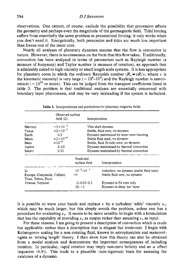
5 94 D J Stevenson
observations. One cannot, of course, exclude the possibility that precession affects the geometry and perhaps even the magnitude of the geomagnetic field. Tidal forcing suffers from essentially the same problem as precessional forcing: it only works when you don’t need it. Energetically, both precession and tides are much less important than freeze-out of the inner core.
Nearly all analyses of planetary dynamos assume that the flow is convective in nature. However, there is no consensus on the form that this flow takes. Traditionally, convection has been analysed in terms of parameters such as Rayleigh number (a measure of buoyancy) and Taylor number (a measure of rotation), an approach that is admirably suited to high viscosity or small length scale systems. It is less appropriate for planetary cores in which the ordinary Reynolds number (Re= v R / v , where v is the kinematic viscosity) is very large ( - 106-108) and the Rayleigh number is astron- omical ( - lo2’ or more). This can be judged from the transport coefficients listed in table 3. The problem is that traditional analyses are essentially concerned with boundary layer phenomena, and may be very misleading if the system is turbulent.
Table 3. Interpretations and predictions for planetary magnetic fields.
Observed surface field (G) Interpretation
Mercury -2 x 10-~ Thin shell dynamo Venus 6 2 x 10 -~ Stable, fluid core; no dynamo Earth 0.3 Dynamo maintained by inner-core freezing Moon s 2 x 10⁻⁶ Stable fluid shell; no dynamo Mars s 10-~ Stable, fluid (S-rich) core; no dynamo Jupiter 4-10 Dynamo maintained by thermal convection Saturn 0.21 Dynamo maintained by thermal convection
Predicted surface field Interpretation
~~~~~~ ~
Io 10-*-10-~ Induction; no dynamo (stable fluid core) Europa, Ganymede, Callisto, -0 Stable fluid core, no dynamo Titan, Triton, Pluto Uranus, Neptune (i) 0.01-0.1 Dynamo in Fe core only
(ii) -1 Dynamo in deep ‘ice’ layer
It is possible to wave your hands and replace v by a turbulent ‘eddy’ viscosity ve, which may be much larger, but this simply avoids the problem, unless one has a procedure for evaluating v,. It seems to be more sensible to begin with a formulation that has the capability of providing v e as output rather than assuming ve as input.
For these reasons, I am going to present a description of convection which is crude but applicable; rather than a description that is elegant but irrelevant. I begin with Kolmogorov scaling for a non-rotating fluid, known to astrophysicists and meteorol- ogists as ‘mixing length’ theory. I then show how this theory can also be obtained from a modal analysis and demonstrate the important consequences of including rotation. In particular, rapid rotation may imply non-zero helicity and an a effect (equation (4.9)). This leads to a plausible (non-rigorous) basis for assessing the existence of a dynamo.
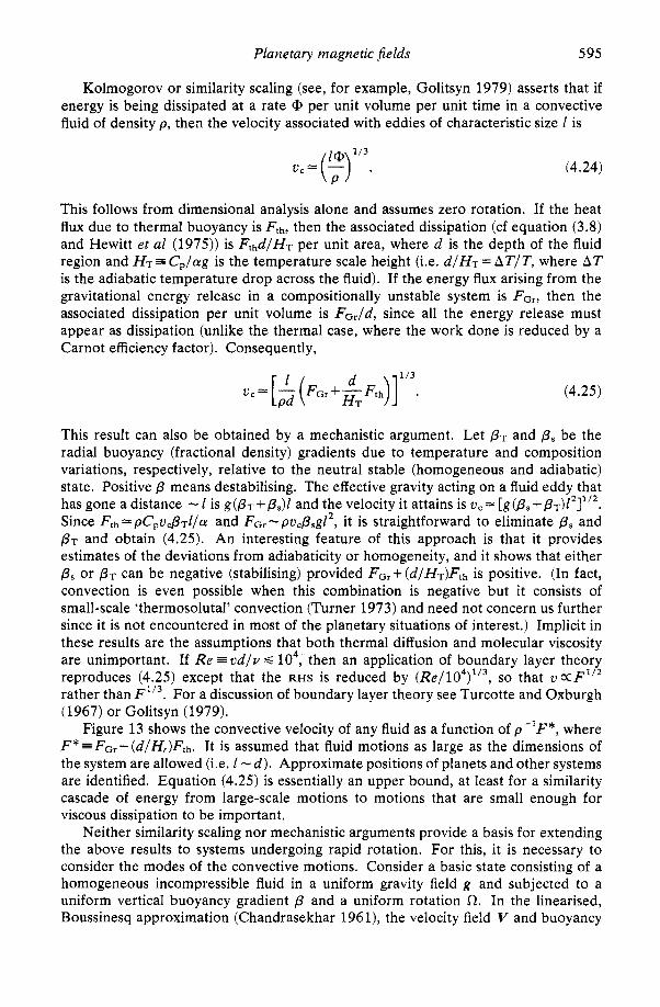
Planetary magnetic fields 595
Kolmogorov or similarity scaling (see, for example, Golitsyn 1979) asserts that if energy is being dissipated at a rate @ per unit volume per unit time in a convective fluid of density p , then the velocity associated with eddies of characteristic size I is
(4.24)
This follows from dimensional analysis alone and assumes zero rotation. If the heat flux due to thermal buoyancy is Fth, then the associated dissipation (cf equation (3.8) and Hewitt et a1 (1975)) is Fthd/HT per unit area, where d is the depth of the fluid region and H T = C p / ~ g is the temperature scale height (i.e. d/HT= ATIT, where AT is the adiabatic temperature drop across the fluid). If the energy flux arising from the gravitational energy release in a compositionally unstable system is F G ~ , then the associated dissipation per unit volume is FG,/d, since all the energy release must appear as dissipation (unlike the thermal case, where the work done is reduced by a Carnot efficieccy factor). Consequently,
(4.25)
This result can also be obtained by a mechanistic argument. Let PT and ps be the radial buoyancy (fractional density) gradients due to temperature and composition variations, respectively, relative to the neutral stable (homogeneous and adiabatic) state. Positive p means destabilising. The effective gravity acting on a fluid eddy that has gone a distance - 1 is g(pT+&)l and the velocity it attains is tic=[g(ps+pT)P]1’2. Since Fth =pCPticpTI/Ly and FGr-pticpsg12, it is straightforward to eliminate ps and pT and obtain (4.25). An interesting feature of this approach is that it provides estimates of the deviations from adiabaticity or homogeneity, and it shows that either ps or pT can be negative (stabilising) provided FGr+(d/HT)Fth is positive. (In fact, convection is even possible when this combination is negative but it consists of small-scale ‘thermosolutal’ convection (Turner 1973) and need not concern us further since it is not encountered in most of the planetary situations of interest.) Implicit in these results are the assumptions that both thermal diffusion and molecular viscosity are unimportant. If R e = ud/v 6 lo4, then an application of boundary layer theory reproduces (4.25) except that the RHS is reduced by ( ~ ? e / l O ~ ) l ’ ~ , so that t i o ~ F ” ~ rather than F1/3 . For a discussion of boundary layer theory see Turcotte and Oxburgh (1967) or Golitsyn (1979).
Figure 13 shows the convective velocity of any fluid as a function of p-’F*, where F* = FGr+ (d/Hr)Fth. It is assumed that fluid motions as large as the dimensions of the system are allowed (i.e. I - d ) . Approximate positions of planets and other systems are identified. Equation (4.25) is essentially an upper bound, at least for a similarity cascade of energy from large-scale motions to motions that are small enough for viscous dissipation to be important.
Neither similarity scaling nor mechanistic arguments provide a basis for extending the above results to systems undergoing rapid rotation. For this, it is necessary to consider the modes of the convective motions. Consider a basic state consisting of a homogeneous incompressible fluid in a uniform gravity field g and subjected to a uniform vertical buoyancy gradient p and a uniform rotation a. In the linearised, Boussinesq approximation (Chandrasekhar 196 l ) , the velocity field V and buoyancy
596 D J Stevenson
Figure 13. The convective velocity of everything (but for zero rotation and zero magnetic field). F* is defined in the text; it is the ‘available’ energy flux. (‘Available’ means that it excludes the conductive flux and incorporates the consequences of the second law of theryodynamics.) The full line is given by (4.24) (zero viscosity). The broken line is for a viscosity of 10’’ P.
perturbation 8 satisfy
1 at P c + 2 0 x v = --Ap-ge (4.26)
Q * V = O (4.27)
ae - = p . v at
(4.28)
assuming thermal diffusivity and molecular viscosity are negligible. For velocity and buoyancy perturbations ccexp (ik * r +ut), the dispersion relation is
u k 2 = gpk: - ( 2 0 * k)2 (4.29)
where gp > 0 in a destabilising case, k = / k / and k, is the horizontal component of k. This result is obtained for a linearised, Boussinesq, incompressible fluid (for example, Flasar and Gierasch 1978, Stevenson 1979). It is clear that in the high rotation limit (a2 >> gp) , growing modes are only possible for wavevectors with small components in the direction of 0. These modes are narrow cylinders or pancakes aligned with the rotation axis. The linear theory can be converted into a crude finite-amplitude theory by asserting that modes cannot grow beyond the amplitude at which secondary, shear instabilities grow more rapidly than the primary (convective) instability. This gives the criterion
u = v k (4.30)
where v is the magnitude of the velocity. This criterion is discussed at length by Flasar and Gierasch (1978) and Stevenson (1979). Similar criteria have been suggested for baroclinic instabilities in planetary atmospheres (Charney 1959). The final step is less well justified and assumes that the preferred mode is the one which maximises the energy transport for a given buoyancy gradient p and specified boundary condi- tions.
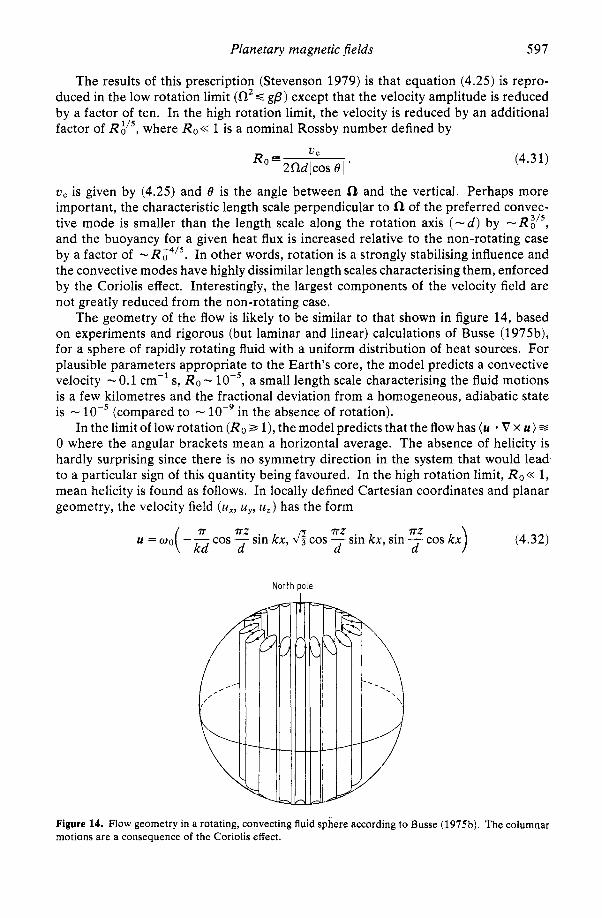
Planetary magnetic fields 597
The results of this prescription (Stevenson 1979) is that equation (4.25) is repro- duced in the low rotation limit (a2 s g p ) except that the velocity amplitude is reduced by a factor of ten. In the high rotation limit, the velocity is reduced by an additional factor of RA’5, where Ro<< 1 is a nominal Rossby number defined by
(4.31)
uC is given by (4.25) and 8 is the angle between fl and the vertical. Perhaps more important, the characteristic length scale perpendicular to of the preferred convec- tive mode is smaller than the length scale along the rotation axis ( - d ) by - R:’5, and the buoyancy for a given heat flux is increased relative to the non-rotating case by a factor of - R04”. In other words, rotation is a strongly stabilising influence and the convective modes have highly dissimilar length scales characterising them, enforced by the Coriolis effect. Interestingly, the largest components of the velocity field are not greatly reduced from the non-rotating case.
The geometry of the flow is likely to be similar to that shown in figure 14, based on experiments and rigorous (but laminar and linear) calculations of Busse (1975b), for a sphere of rapidly rotating fluid with a uniform distribution of heat sources. For plausible parameters appropriate to the Earth’s core, the model predicts a convective velocity - 0.1 cm-’ s, Ro - a small length scale characterising the fluid motions is a few kilometres and the fractional deviation from a homogeneous, adiabatic state is - lo-’ (compared to - in the absence of rotation).
In the limit of low rotation (Ro 3 l ) , the model predicts that the flow has ( U * V x U ) = 0 where the angular brackets mean a horizontal average. The absence of helicity is hardly surprising since there is no symmetry direction in the system that would lead to a particular sign of this quantity being favoured. In the high rotation limit, Roc< 1, mean helicity is found as follows. In locally defined Cartesian coordinates and planar geometry, the velocity field ( u ~ , U,, U,) has the form
) (4.32) 2 =z 7TZ
d d sin kx, d, cos - sin kx, sin - cos kx
North pole
Figure 14. Flow geometry in a rotating, convecting fluid sphere according to Busse (1975b). The columnar motions are a consequence of the Coriolis effect.
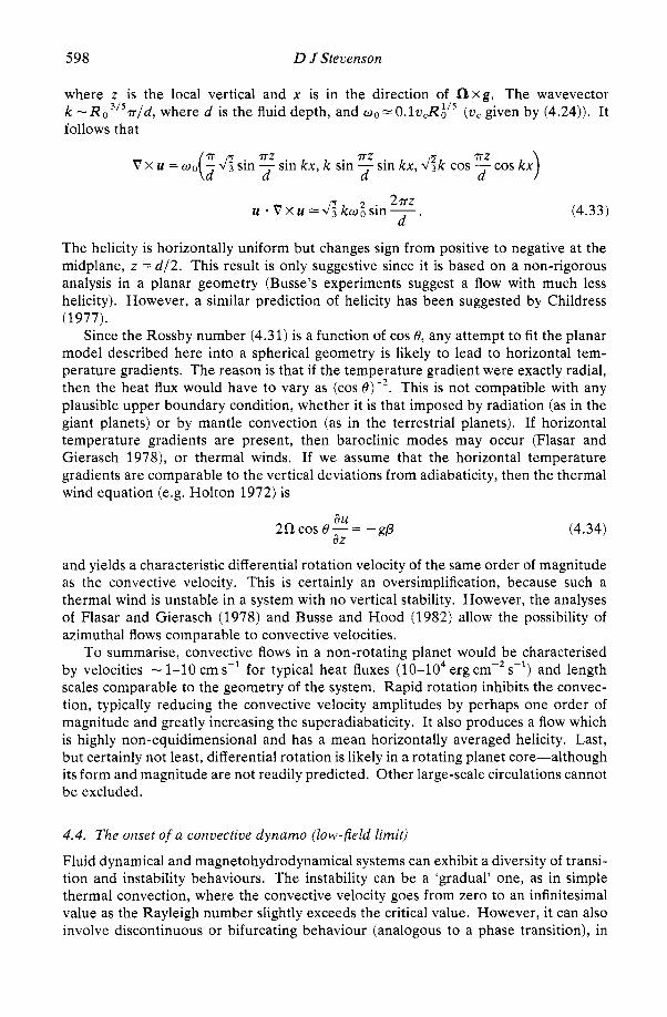
598 D JStevenson
where z is the local vertical and x is in the direction of n x g . The wavevector k - R 6 3 ’ 5 ~ / d , where d is the fluid depth, and uo=0.1v,RA’5 (U, given by (4.24)). It follows that
7Tz 7TZ z 7TZ
d d d V x U = uo( 3 J5 sin - sin kx, k sin - sin kx, JTk cos - cos kx
U * V x U = ./$ ku: sin - , -
(4.33) 27Tz d
The helicity is horizontally uniform but changes sign from positive to negative at the midplane, z = d / 2 . This result is only suggestive since it is based on a non-rigorous analysis in a planar geometry (Busse’s experiments suggest a flow with much less helicity). However, a similar prediction of helicity has been suggested by Childress (1977).
Since the Rossby number (4.31) is a function of cos 8, any attempt to fit the planar model described here into a spherical geometry is likely to lead to horizontal tem- perature gradients. The reason is that if the temperature gradient were exactly radial, then the heat flux would have to vary as (cos This is not compatible with any plausible upper boundary condition, whether it is that imposed by radiation (as in the giant planets) or by mantle convection (as in the terrestrial planets). If horizontal temperature gradients are present, then baroclinic modes may occur (Flasar and Gierasch 1978), or thermal winds. If we assume that the horizontal temperature gradients are comparable to the vertical deviations from adiabaticity, then the thermal wind equation (e.g. Holton 1972) is
(4.34) au
COS^-= -gp az
and yields a characteristic differential rotation velocity of the same order of magnitude as the convective velocity. This is certainly an oversimplification, because such a thermal wind is unstable in a system with no vertical stability. However, the analyses of Flasar and Gierasch (1978) and Busse and Hood (1982) allow the possibility of azimuthal flows comparable to convective velocities.
To summarise, convective flows in a non-rotating planet would be characterised by velocities - 1-10 cm s-l for typical heat fluxes (10-104 erg cmP2 s-I) and length scales comparable to the geometry of the system. Rapid rotation inhibits the convec- tion, typically reducing the convective velocity amplitudes by perhaps one order of magnitude and greatly increasing the superadiabaticity. It also produces a flow which is highly non-equidimensional and has a mean horizontally averaged helicity. Last, but certainly not least, differential rotation is likely in a rotating planet core-although its form and magnitude are not readily predicted. Other large-scale circulations cannot be excluded.
4.4. The onset of a convective dynamo (low-field limit)
Fluid dynamical and magnetohydrodynamical systems can exhibit a diversity of transi- tion and instability behaviours. The instability can be a ‘gradual’ one, as in simple thermal convection, where the convective velocity goes from zero to an infinitesimal value as the Rayleigh number slightly exceeds the critical value. However, it can also involve discontinuous or bifurcating behaviour (analogous to a phase transition), in
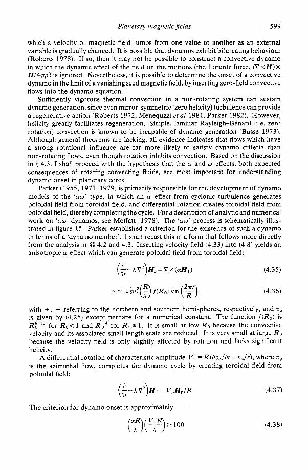
Planetary magnetic fields 599
which a velocity or magnetic field jumps from one value to another as an external variable is gradually changed. It is possible that dynamos exhibit bifurcating behaviour (Roberts 1978). If so, then it may not be possible to construct a convective dynamo in which the dynamic effect of the field on the motions (the Lorentz force, (V X H) X
H/47rp) is ignored. Nevertheless, it is possible to determine the onset of a convective dynamo in the limit of a vanishing seed magnetic field, by inserting zero-field convective flows into the dynamo equation.
Sufficiently vigorous thermal convection in a non-rotating system can sustain dynamo generation, since even mirror-symmetric (zero helicity) turbulence can provide a regenerative action (Roberts 1972, Menequzzi et a1 1981, Parker 1982). However, helicity greatly facilitates regeneration. Simple, laminar Rayleigh-BCnard (i.e. zero rotation) convection is known to be incapable of dynamo generation (Busse 1973). Although general theorems are lacking, all evidence indicates that flows which have a strong rotational influence are far more likely to satisfy dynamo criteria than non-rotating flows, even though rotation inhibits convection. Based on the discussion in 9 4.3, I shall proceed with the hypothesis that the a and w effects, both expected consequences of rotating convecting fluids, are most important for understanding dynamo onset in planetary cores.
Parker (1955, 1971, 1979) is primarily responsible for the development of dynamo models of the “J’ type, in which an a effect from cyclonic turbulence generates poloidal field from toroidal field, and differential rotation creates toroidal field from poloidal field, thereby completing the cycle. For a description of analytic and numerical work on ‘ a w ’ dynamos, see Moffatt (1978). The ‘ aw ’ process is schematically illus- trated in figure 15. Parker established a criterion for the existence of such a dynamo in terms of a ‘dynamo number’. I shall recast this in a form that follows more directly from the analysis in § § 4.2 and 4.3. Inserting velocity field (4.33) into (4.8) yields an anisotropic a effect which can generate poloidal field from toroidal field:
(:-A V)H, = v x (aHT) (4.35)
(4.36)
with +, - referring to the northern and southern hemispheres, respectively, and uC is given by (4.25) except perhaps for a numerical constant. The function f(R0) is R;’” for R o c 1 and R04 for R0a 1. It is small at low Ro because the convective velocity and its associated small length scale are reduced. It is very small at large Ro because the velocity field is only slightly affected by rotation and lacks significant helicity.
R (au,/ar - u,/T), where U ,
is the azimuthal flow, completes the dynamo cycle by creating toroidal field from poloidal field:
A differential rotation of characteristic amplitude V,
($ - A v ~ ) H ~ = V, H , / R . (4.37)
The criterion for dynamo onset is approximately
(F)(T) V,R b 100 (4.38)
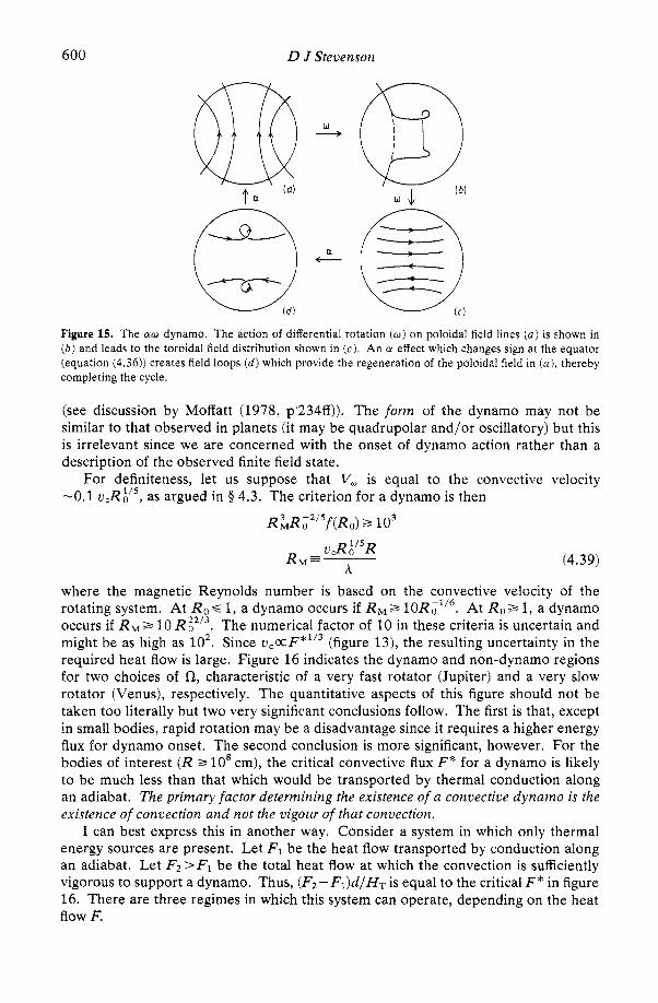
600 D J Stevenson
a c-
Figure 15. The LYU dynamo. The action of differential rotation ( U ) on poloidal field lines (a) is shown in ( b ) and leads to the toroidal field distribution shown in ( c ) . An a effect which changes sign at the equator (equation (4.36)) creates field loops ( d ) which provide the regeneration of the poloidal field in ( a ) , thereby compieting the cycle.
(see discussion by Moffatt (1978, p’234ff)). The form of the dynamo may not be similar to that observed in planets (it may be quadrupolar and/or oscillatory) but this is irrelevant since we are concerned with the onset of dynamo action rather than a description of the observed finite field state.
For definiteness, let us suppose that V, is equal to the convective velocity -0.1 v ,R~/ ’ , as argued in § 4.3. The criterion for a dynamo is then
R hR i2”f (Ro) b lo3
(4.39)
where the magnetic Reynolds number is based on the convective velocity of the rotating system. At R o c 1, a dynamo occurs if R M b 10R;’16. At Rob 1, a dynamo occurs if R M a 10 The numerical factor of 10 in these criteria is uncertain and might be as high as lo2. Since v , o ; F * ~ / ~ (figure 13), the resulting uncertainty in the required heat flow is large. Figure 16 indicates the dynamo and non-dynamo regions for two choices of Cl, characteristic of a very fast rotator (Jupiter) and a very slow rotator (Venus), respectively. The quantitative aspects of this figure should not be taken too literally but two very significant conclusions follow. The first is that, except in small bodies, rapid rotation may be a disadvantage since it requires a higher energy flux for dynamo onset. The second conclusion is more significant, however. For the bodies of interest (R b lo8 cm), the critical convective flux F* for a dynamo is likely to be much less than that which would be transported by thermal conduction along an adiabat. The primary factor determining the existence of a convective dynamo is the existence of convection and not the vigour of that convection.
I can best express this in another way. Consider a system in which only thermal energy sources are present. Let F1 be the heat flow transported by conduction along an adiabat. Let F2>F1 be the total heat flow at which the convection is sufficiently vigorous to support a dynamo. Thus, ( F 2 - F l ) d / H T is equal to the critical F* in figure 16. There are three regimes in which this system can operate, depending on the heat flow F.
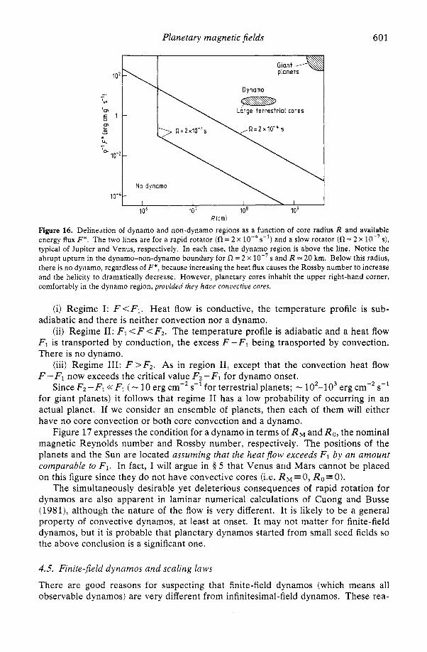
Planetary magnetic fields 60 1
Rlcml
Figure 16. Delineation of dynamo and non-dynamo regions as a function of core radius R and available energy flux F*. The two lines are for a rapid rotator (n = 2 x s-') and a slow rotator (n = 2 X lO-'s), typical of Jupiter and Venus, respectively. In each case, the dynamo region is above the line. Notice the abrupt upturn in the dynamo-non-dynamo boundary for = 2 x lO.-'s and R = 20 km. Below this radius, there is no dynamo, regardless of F*, because increasing the heat flux causes the Rossby number to increase and the helicity to dramatically decrease. However, planetary cores inhabit the upper right-hand corner, comfortably in the dynamo region, provided they have convecrive cores.
(i) Regime I: F < F1. Heat flow is conductive, the temperature profile is sub- adiabatic and there is neither convection nor a dynamo.
(ii) Regime 11: F1 < F < F2. The temperature profile is adiabatic and a heat flow F1 is transported by conduction, the excess F - F1 being transported by convection. There is no dynamo.
(iii) Regime 111: F >F2. As in region 11, except that the convection heat flow F - F1 now exceeds the critical value F2 - F1 for dynamo onset.
Since F2 - F1 << F1 ( - 10 erg cm-' s-' for terrestrial planets; - 102-103 erg cm-* sC1 for giant planets) it follows that regime I1 has a low probability of occurring in an actual planet. If we consider an ensemble of planets, then each of them will either have no core convection or both core convection and a dynamo.
Figure 17 expresses the condition for a dynamo in terms of R M and Ro, the nominal magnetic Reynolds number and Rossby number, respectively. The positions of the planets and the Sun are located assuming that the heat flow exceeds F1 by an amount comparable to F1. In fact, I will argue in Q 5 that Venus and Mars cannot be placed on this figure since they do not have convective cores (i.e. R M = 0, Ro = 0).
The simultaneously desirable yet deleterious consequences of rapid rotation for dynamos are also apparent in laminar numerical calculations of Cuong and Busse (1981), although the nature of the flow is very different. It is likely to be a general property of convective dynamos, at least at onset. It may not matter for finite-field dynamos, but it is probable that planetary dynamos started from small seed fields so the above conclusion is a significant one.
4.5. Finite-Feld dynamos and scaling laws
There are good reasons for suspecting that finite-field dynamos (which means all observable dynamos) are very different from infinitesimal-field dynamos. These rea-
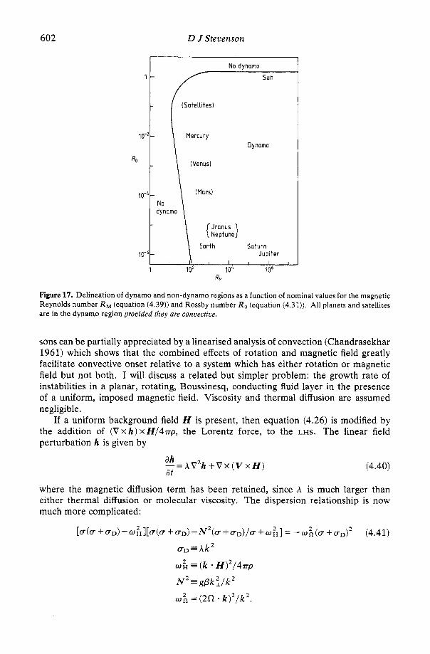
602
1 -
D J Stevenson
No dynamo
Sun
sons can be partially appreciated by a linearised analysis of convection (Chandrasekhar 1961) which shows that the combined effects of rotation and magnetic field greatly facilitate convective onset relative to a system which has either rotation or magnetic field but not both. I will discuss a related but simpler problem: the growth rate of instabilities in a planar, rotating, Boussinesq, conducting fluid layer in the presence of a uniform, imposed magnetic field. Viscosity and thermal diffusion are assumed negligible.
If a uniform background field H is present, then equation (4.26) is modified by the addition of ( V x h ) x H / 4 r p , the Lorentz force, to the LHS. The linear field perturbation h is given by
ah= AV’h + V x (V x H) a t
(4.40)
where the magnetic diffusion term has been retained, since A is much larger than either thermal diffusion or molecular viscosity. The dispersion relationship is now much more complicated:
[U(U +UD) +Ui][c+(CT +CTD)-N’(CT +UJJ)/U +OH]= 2 - U i ( U +UD)’ (4.41) 2 UD=Ak
U L E (k - H)2/4.1rp
N 2 = g p k : / k 2
U: = (2ll 6 k)’/k’.
Planetary magnetic fields 603
In the dissipationless limit ( I C T ~ > > vD), this equation describes MAC waves (Roberts and Soward 1972) as well as unstable states. An unstable solution exists for all buoyant states (i.e. all N 2 > 0) provided vD is finite. The fastest growing mode occurs at U& = 0 provided U: s N 2 / 2 . However, the fastest growing mode occurs at finite field (U& > O ) whenever rotation is large, i.e. U: >N2/2 . In the finite-amplitude extension of the theory (equation (4.30)) a similar conclusion holds (Stevenson 1979): the largest heat flux (or the lowest temperature gradient for a given heat flux) occurs at non-zero field, provided the rotation rate is sufficiently rapid (Ro s 0.1). In this context, all planets are rapid rotators. The physics is this: in the absence of a magnetic field, the Coriolis force must be balanced by horizontal pressure gradients. This enforces at least one small horizontal length scale on the flow and makes convection more difficult. When a significant magnetic field is present, part of the Coriolis force can be balanced by part of the Lorentz force. Horizontal pressure gradients are reduced and it is no longer necessary to have a small horizontal length scale in the convective flow, thereby making the convection ‘easier’.
There is an ‘optimal’ field for which the temperature gradient is least for a given heat flux. In the dissipative limit (vD >>N), this field is given by (Stevenson 1979)
In the dissipationless limit (vD K N ) , the optimal field
(4.42)
(4.43)
These apply to the largest field component, probably the toroidal field. None of these calculations are directly applicable to the dynamo problem because the applied field is uniform and thus has not been incorporated into any finite geometry such as a sphere. Nevertheless, the results suggest the following magnetohydrodynamic transi- tion: once the criterion for dynamo onset is satisfied, the field begins to grow. The Lorentz force relaxes the constraint on the convection imposed by the Coriolis force and causes the convection to become more vigorous. The system continues unstably until it encounters a new stable state at or near the ‘optimal’ field. This state has the property that the flow dimensions are almost equidimensional (just as in non-rotating, zero H Rayleigh-Btnard convection). However, it is possible that some dynamos cannot achieve this ‘optimal’ state for energetic reasons (see below).
A more rigorous (but laminar) analysis of this problem has been made, primarily by Soward (1979), but see also Fearn (1979). They find that the ratio H2/8*pAa, suggested by equation (4.42), is the critical parameter for explaining and characterising convection in the presence of both magnetic field and rotation. When this ratio is of the order of unity, convection is more efficient than elsewhere. Near zero field, there might be a small region of dynamo stability of the type envisaged by Busse (1975b) in his ‘geodynamo’ but this would exist only by virtue of other dissipative processes (thermal diffusion, viscosity) and is unlikely to be important in planets where A is larger than K or v by -six orders of magnitude.
The work of Malkus and Proctor (1975) and Proctor (1977a, b) illustrates another important aspect of large-field dynamos: the consequences of the Lorentz force and the Taylor constraint (Taylor 1963). This constraint concerns zonal Lorentz torques which cannot be balanced by Coriolis forces, and it can be satisfied by adding a ‘free’ zonal Row to the velocity field. (‘Free’ means that it trivially satisfies 2 0 x V = - (l/p)Vp.) Malkus and Proctor found that the large-scale flow driven by the large-scale
604 D J Stevenson
Lorentz force can inhibit further dynamo amplification once H’ - 87rpA 0, exactly the same ‘critical’ field as that discussed above.
In the Earth, this ‘optimal’ field is -20 G, larger than the likely poloidal field at the core-mantle boundary ( - 5-10 G) but smaller than many estimates of the core toroidal field (100-300G (Hide and Roberts 1979)). However, the optimal field suggested by (4.42) is only - 2 G for the metallic hydrogen core of Jupiter; certainly less than even the poloidal field, which is - 10-10’ G in the core (depending on the strength of higher-order multipoles). The dissipationless case, equation (4.43), predicts 102-103 G, which is more reasonable and more consistent with the assumptions, given that R M is very large ( - lo7) in Jupiter. Alternatively, the observed field is generated in a lower conductivity region outside the metallic core (Hide 1967).
One desired outcome of a complete dynamo theory would be a ‘scaling law’ relating the observed field strength to other relevant observable or microscopic properties of a planet (R, 0, A, p, F*, . . .). Scaling laws have been discussed frequently in the literature (e.g. Hide 1974, Rochester et a1 1975, Busse 1976a, Jacobs 1979). The above two examples of Earth and Jupiter illustrate the primary pitfall of any proposed scaling law, including the ‘magnetic Bode’s law’ (e.g. Russell 1979a). The planets are probably too dissimilar for any single scaling law to apply. I can best illustrate this by a consideration of energy balance. The ‘scaling laws’ (4.42) and (4.43) are dynamically determined and represent the optimal balance of Coriolis and Lorentz forces. However, there is another constraint on the field imposed by the first and second laws of thermodynamics (Hewitt et a1 1975, Gubbins 1977a):
(4.44) d
A (v X HI2 d V Q G r + r/(-)Qtj, Ht
where the LHS is the Ohmic dissipation in the dynamo, QGr is the gravitational energy release (e.g. from the upward displacement of light fluid elements as the inner core of the Earth grows), Qth is the thermal energy release and q is a numerical factor depending on the distribution of this energy release (7 = 1 for heat release at the bottom, 77 = 0.3-0.4 for distributed heat release). The factor r/d/HT is essentially the Carnot efficiency of the system. (The assertion that all of the gravitational energy release QGI is available for dynamo generation, and hence Ohmic dissipation, assumes only large-scale motions and might possibly be wrong.) If it is assumed that the Ohmic dissipation is associated with large-scale currents, then (4.44) leads to an estimate of the Earth’s toroidal field which ranges from 10-300 G, depending on assumptions made (Gubbins 1977a, Loper 1978, Gubbins et a1 1979). The important point is that equation (4.42), which contains no information about the energy source responsible for the dynamo, gives a comparable field amplitude. This is a coincidence. It also highlights the dangers inherent in scaling laws, especially when applied to terrestrial planets. Application of equation (4.44) to Jupiter yields a characteristic field amplitude of - 105.5 G, almost five orders of magnitude greater than the ‘optimal’ field (4.42), and three orders of magnitude larger than the dissipationless formula (4.43)! The difference arises because dissipation in Jupiter is probably associated with small-scale currents.
There are many different ways of getting approximately the right field amplitude for the Earth from the available parameters. For example, uC is comparable to (A 0)*”, so any scaling law can be modified by including powers of v , / ( A ~ ) ” 2 without significantly altering its ability to describe the field amplitude. Clearly, the Earth is not a good choice for testing scaling laws. It might be supposed that Mercury is a
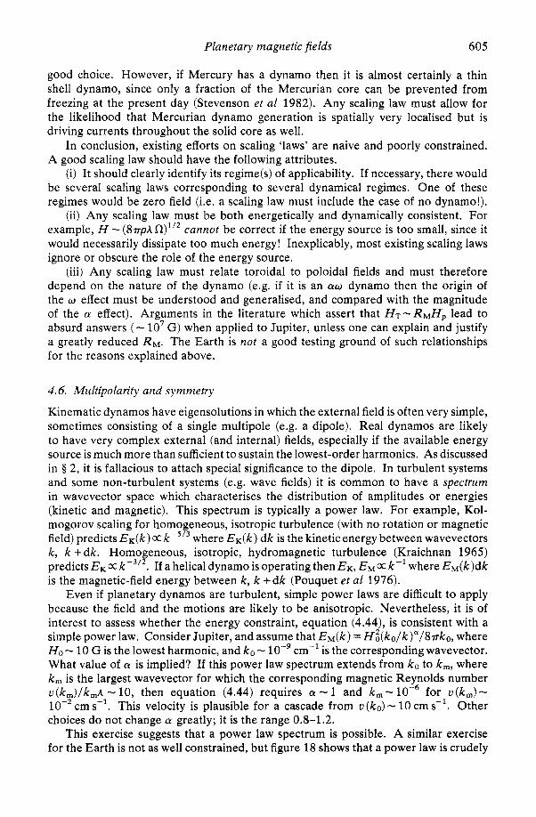
Plunetary magnetic fields 605
good choice. However, if Mercury has a dynamo then it is almost certainly a thin shell dynamo, since only a fraction of the Mercurian core can be prevented from freezing at the present day (Stevenson et a1 1982). Any scaling law must allow for the likelihood that Mercurian dynamo generation is spatially very localised but is driving currents throughout the solid core as well.
In conclusion, existing efforts on scaling 'laws' are naive and poorly constrained. A good scaling law should have the following attributes.
(i) It should clearly identify its regime(s) of applicability. If necessary, there would be several scaling laws corresponding to several dynamical regimes. One of these regimes would be zero field (i.e. a scaling law must include the case of no dynamo!).
(ii) Any scaling law must be both energetically and dynamically consistent. For example, H - ( 8 7 ~ p h f i ) ' / ~ cannot be correct if the energy source is too small, since it would necessarily dissipate too much energy! Inexplicably, most existing scaling laws ignore or obscure the role of the energy source.
(iii) Any scaling law must relate toroidal to poloidal fields and must therefore depend on the nature of the dynamo (e.g. if it is an aw dynamo then the origin of the w effect must be understood and generalised, and compared with the magnitude of the a effect). Arguments in the literature which assert that HT-RMH, lead to absurd answers ( - lo' G) when applied to Jupiter, unless one can explain and justify a greatly reduced R M . The Earth is not a good testing ground of such relationships for the reasons explained above.
4.6. Multipolarity and symmetry
Kinematic dynamos have eigensolutions in which the external field is often very simple, sometimes consisting of a single multipole (e.g. a dipole). Real dynamos are likely to have very complex external (and internal) fields, especially if the available energy source is much more than sufficient to sustain the lowest-order harmonics. As discussed in § 2, it is fallacious to attach special significance to the dipole. In turbulent systems and some non-turbulent systems (e.g. wave fields) it is common to have a spectrum in wavevector space which characterises the distribution of amplitudes or energies (kinetic and magnetic). This spectrum is typically a power law. For example, Kol- mogorov scaling for homogeneous, isotropic turbulence (with no rotation or magnetic field) predicts E K ( k ) cc k -5'3 where EK(k) dk is the kinetic energy between wavevectors k, k + dk. Homogeneous, isotropic, hydromagnetic turbulence (Kraichnan 1965) predictsEKE kP3I2 . If a helical dynamo is operating then EK, EM= k-' where EM(k)dk is the magnetic-field energy between k , k +dk (Pouquet et al 1976).
Even if planetary dynamos are turbulent, simple power laws are difficult to apply because the field and the motions are likely to be anisotropic. Nevertheless, it is of interest to assess whether the energy constraint, equation (4.44), is consistent with a simple power law. Consider Jupiter, and assume that E&) = HE(ko/k)"/8~ko, where Ho - 10 G is the lowest harmonic, and ko - cm-' is the corresponding wavevector. What value of a is implied? If this power law spectrum extends from ko to k,, where k, is the largest wavevector for which the corresponding magnetic Reynolds number U (k,)/k,h - 10, then equation (4.44) requires a - 1 and k, - low6 for U (k,) - lo-' cm s-'. This velocity is plausible for a cascade from v ( k o ) - 10 cm s-', Other choices do not change a greatly; it is the range 0.8-1.2.
This exercise suggests that a power law spectrum is possible. A similar exercise for the Earth is not as well constrained, but figure 18 shows that a power law is crudely
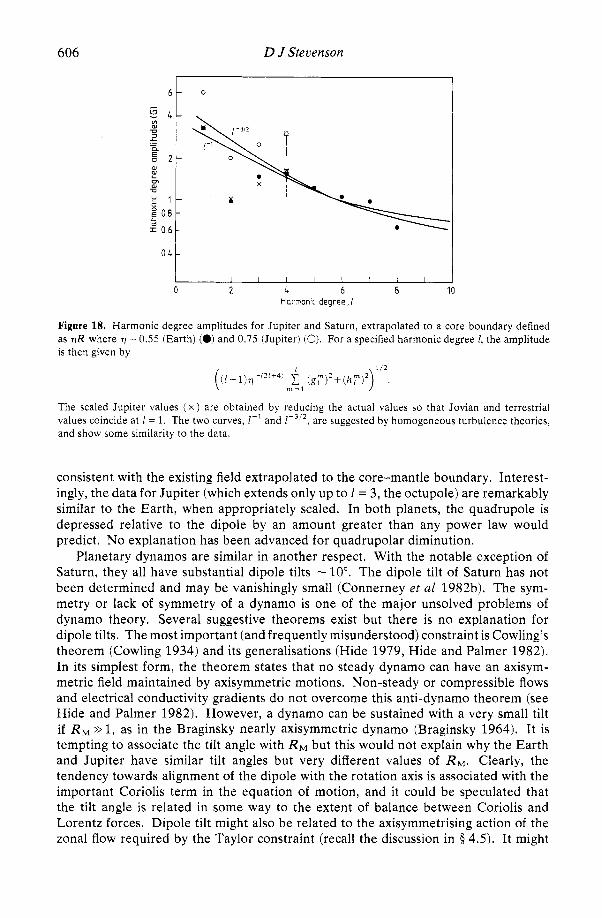
606 D J Stevenson
t I I 1 I I I I I 1
0 2 4 6 0 1 Harmonic degree, 1
Figure 18. Harmonic degree amplitudes for Jupiter and Saturn, extrapolated to a core boundary defined as qR where 7 = 0.55 (Earth) (0) and 0.75 (Jupiter) (0). For a specified harmonic degree I , the amplitude is then given by
The scaled Jupiter values ( X ) are obtained by reducing the actual values so that Jovian and terrestrial values coincide at I = 1. The two curves, I - ' and are suggested by homogeneous turbulence theories, and show some similarity to the data.
consistent with the existing field extrapolated to the core-mantle boundary. Interest- ingly, the data for Jupiter (which extends only up to 1 = 3, the octupole) are remarkably similar to the Earth, when appropriately scaled. In both planets, the quadrupole is depressed relative to the dipole by an amount greater than any power law would predict. No explanation has been advanced for quadrupolar diminution.
Planetary dynamos are similar in another respect. With the notable exception of Saturn, they all have substantial dipole tilts - 10". The dipole tilt of Saturn has not been determined and may be vanishingly small (Connerney et a1 1982b). The sym- metry or lack of symmetry of a dynamo is one of the major unsolved problems of dynamo theory. Several suggestive theorems exist but there is no explanation for dipole tilts. The most important (and frequently misunderstood) constraint is Cowling's theorem (Cowling 1934) and its generalisations (Hide 1979, Hide and Palmer 1982). In its simplest form, the theorem states that no steady dynamo can have an axisym- metric field maintained by axisymmetric motions. Non-steady or compressible flows and electrical conductivity gradients do not overcome this anti-dynamo theorem (see Hide and Palmer 1982). However, a dynamo can be sustained with a very small tilt if R M > > l , as in the Braginsky nearly axisymmetric dynamo (Braginsky 1964). It is tempting to associate the tilt angle with RM but this would not explain why the Earth and Jupiter have similar tilt angles but very different values of RM. Clearly, the tendency towards alignment of the dipole with the rotation axis is associated with the important Coriolis term in the equation of motion, and it could be speculated that the tilt angle is related in some way to the extent of balance between Coriolis and Lorentz forces. Dipole tilt might also be related to the axisymmetrising action of the zonal flow required by the Taylor constraint (recall the discussion in B 4.5). It might
Planetary magnetic fields 607
even be related to the number of large-scale convective cells (recall that this is small if the Coriolis and Lorentz forces are comparable).
Reduction of tilt is easier to understand than the existence of tilt. Axisymmetric differential rotation is effective in reducing non-axisymmetric field components, essen- tially because of the electromagnetic skin effect (Thomson 1893, Herzenberg and Lowes 1957, Crane 1974, Stevenson 1982b). The latter paper uses this to explain Saturn (see § 5).
4.7. Time variability and reversals
The Earth’s magnetic field varies in geometry and strength over all time scales from 10-109yr. (It may even vary on shorter time scales, but these variations would be undetectable because of screening by the conductivity of the deep mantle.) Insufficient data exist to assess whether other planetary dynamos vary. A diversity of possible dynamic or diffusive time scales exist for a planetary core: gravitational or seismic (acoustic), rotation (inertial waves), hydromagnetic waves, convection and circulation, magnetic diffusion, thermal diffusion and viscous diffusion. The first two and last two are too short and too long, respectively, to be of much interest. Hydromagnetic waves (equation (4.41) with uD << / V I ) ) are AlfvCn-like at small wavelengths (w = - iu = w H ) but are highly dispersive and much slower at large wavelengths (w - w h / w n ) . The ‘slow’ hydromagnetic wave has a characteristic transit time of - lo3 yr for both Earth and Jupiter (assuming H - lo2 G) and has been invoked by Hide (1966) to explain westward drift of the non-dipole geomagnetic field. Convective time scales are - R/v, and are plausibly 102-103 yr for the Earth, but nearer 10 yr for Jupiter. The similarity of hydromagnetic and convective time scales for the Earth arises for the same reasons that make the Earth a bad test of scaling laws (04.5). The difference for Jupiter emphasises the need to detect secular variation for that planet. If the variation time scale is - 10 yr then at least some of the variability may be attributable to fluctuations in convection.
The magnetic diffusion time is much longer for all planets, and this enabled Hide (1978) to construct a theorem providing a magnetic technique for determining the size of a planet’s conducting core. The theorem assumes ‘frozen flux’ (i.e. negligible magnetic diffusion on the time scale of observation) and asserts that the unsigned flux (or, equivalently, the number of flux lines) through the core boundary does not change with time. This is essentially the theorem of Bondi and Gold (1950). By comparing magnetic-field models at different but closely spaced epochs, it is possible to find the radius at which the downward extrapolation of the field satisfies this frozen flux hypothesis. If the hypothesis is valid then the radius thereby determined is the radius of the core. The application of this theorem to the Earth has proved to be less straightforward than first supposed (Hide and Malin 1981) but appears to reproduce the seismically determined core radius. The attempted application to Jupiter (Hide and Malin 1979) was probably premature. However, there is no doubt that this theorem is important and useful, and the eventual application to more complete planetary data is awaited with interest.
The most spectacular time variability of a dynamo is, of course, reversal. Whereas the solar dynamo reverses on a time scale characteristic of fluid motions (-10 yr), the geodynamo reverses on a time scale (-105-106 yr) that is not clearly related to any time scale listed above but is closest to the magnetic diffusion time ( - lo4 yr). Many ideas have been proposed to explain geomagnetic reversal but no convincing explana-
608 D J Stevenson
tion has emerged. Kinematic reversal schemes include those of Levy (1972a, b). However, it is not even known whether reversals are externally induced (e.g. by small variations in Earth rotation) or are intrinsic to the dynamo process. Once again, a long-term analysis of the Jovian dynamo may prove important. If the reversal process is dynamic then this dynamo may reverse in less than -10’ yr (this is somewhat like predicting the next large earthquake on the San Andreas fault!). If the magnetic diffusion time is relevant then we are doomed to a long wait (-lo9 yr). One aspect of geomagnetic reversals may have important implications for all planetary dynamos. Merrill et a1 (1979) discuss paleomagnetic data and show that the field geometries of normal and reversed polarity states are different. It is as though part of the field is ‘standing’ and does not participate in the reversal. This is an astonishing result since the dynamo equation and magnetohydrodynamic Navier-Stokes equation are both unchanged when W is replaced by -H. If the normal and reversed fields are different in form (and not merely different in sign) this can only mean that the equations admit more than one state. There are at least two states H I and H2, with H2 similar (but not equal to) -H1, and transitions H I @HZ are possible but transitions PI1 @ - H I , H z @ -H2 are not possible. The significance of this for dynamo theory remains obscure but may have to do with the possibility of bifurcating behaviour in magnetohydrody- namic systems (Roberts 1978).
5. The synthesis
Interpretations and predictions are offered here for each of the planets and large satellites, based on the observations and theory presented above. In view of the uncertainties, especially in the application of dynamo theory, this attempted synthesis has a subjective element, but it is based on the following guiding principles.
(i) All planets (and probably all Moon-sized satellites) possess fluid, metallic regions. In the terrestrial planets and satel!ites, these exist because of the eutectic behaviour of iron alloys. In giant planets, these exist because of pressure metallisation in fluid hydrogen or ‘ice’.
(ii) If convection (thermal or compositional) exists in such a fluid metallic region then a dynamo will occur. All planetary bodies (including satellites) rotate fast enough for the Coriolis force to be important, and any plausible vigour of convection is likely to satisfy the magnetic Reynolds number criterion, unless the fluid layer is very small in radial extent.
(iii) In terrestrial bodies, present-day core convection requires inner-core freeze- out, since secular cooling is insufficient to exceed conductive heat transport for an adiabatic state, and intrinsic (radiogenic) heat sources are unlikely. In giant planets, thermal convection is likely from gradual cooling alone, except possibly in the ice layers of Uranus and Neptune.
The results of the synthesis are summarised in table 3.
5.1, Mercury
The most probable explanation for the Mercurian field is a thin shell dynamo, maintained by a chemical convection and latent heat release as the core continues to freeze (Stevenson et a1 1982). As illustrated in figure 6 , the remaining fluid region in Mercury is likely to be thin (-few hundred kilometres in depth, at most) because
Planetary magnetic fields 609
Mercury formed close to the Sun and is therefore not likely to have incorporated much sulphur, a volatile element under early Solar-System conditions. Complete freeze-out of a Mercurian core is prevented by the very low eutectic temperature of Fe-S and the tendency of the overlying mantle to self-regulate by subsolidus convection at a higher temperature.
The dynamo may be energetically marginal, perhaps explaining why the observed field is small. Latent heat release is not sufficient by itself to maintain convection in the fluid shell. Gravitational energy release is small because the distance through which the light alloying constituent is redistributed during core freezing is small. Expressed as a flux (energy release per unit area), the gravitational energy release is FG* = 0.1-0.2(d/100 km)’ erg cm-’s-’ where d is the fluid layer depth. The heat flux by conduction along the adiabat is about 10 erg cm-’s-l; only about half of this can be supplied by latent heat and secular cooling. In accordance with equations (3.7) and (3.8), the existence of convection sustained by compositional buoyancy requires
O.l(d/lOO km)2 b 5(AT/T) = O.l(d/lOO km) (5.1)
which is satisfied for d b 100 km. Energy in excess of the amount required to maintain adiabaticity is available, at least in principle, to sustain a dynamo. (Some fraction is dissipated viscously at small scales.) Even for fluid layers only slightly in excess of criticality, a convective velocity approaching 0.1 cm s-’ is possible and so RM b 10 and Ro =s 1, as required for a dynamo. The maximum available energy for the dynamo is at most about four orders of magnitude less than that available to drive the Earth’s magnetic field. The Ohmic dissipation in Mercury, @Ohm, is given by
@ o h m = A (V X H ) 2 d V J = 4.rr3AH2R2/d
assuming the dissipation is dominated by currents within the fluid shell of characteristic length scale d and associated field amplitude B, (Currents in the inner solid core dissipate less energy for the same field because of a larger associated length scale R, even though they occupy a larger volume.) Equating @Ohm to the available gravitational energy yields - 0.1-1 G, presumably the toroidal field. If the poloidal field is a factor -50 smaller, then the observed field could thereby be explained.
An important feature of Mercury is that the dynamically preferred field (equation (4.43)) --(8.rrpA is -2 G and may not be energetically attainable. This difficulty is not encountered in any of the other planets and suggests that the Mercurian dynamo may be dynamically different from other planetary dynamos. For that reason alone, it is important that further measurements be made of the Mercurian field. It is predicted that Mercury should have a rich multipolar magnetic-field spectrum exter- nally because the depth of field generation is only -500-700 km below the planet surface. It is also expected that the existence of a fluid shell should affect the rotational state and this effect is potentially observable by a Mercury orbiter spacecraft (Peale 1981).
5.2. Venus
The most probable state for Venus, consistent with the absence of a substantial magnetic field, is a stably stratified, completely fluid core. Thermal evolution calcula-
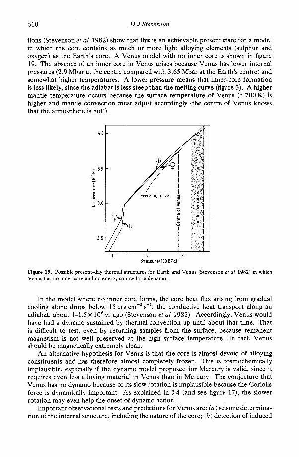
610 D J Stevenson
tions (Stevenson et a1 1982) show that this is an achievable present state for a model in which the core contains as much or more light alloying elements (sulphur and oxygen) as the Earth’s core. A Venus model with no inner core is shown in figure 19. The absence of an inner core in Venus arises because Venus has lower internal pressures (2.9 Mbar at the centre compared with 3.65 Mbar at the Earth’s centre) and somewhat higher temperatures. A lower pressure means that inner-core formation is less likely, since the adiabat is less steep than the melting curve (figure 3). A higher mantle temperature occurs because the surface temperature of Venus (-700 K) is higher and mantle convection must adjust accordingly (the centre of Venus knows that the atmosphere is hot!).
1 2 3 Pressure(100 GPai
Figure 19. Possible present-day thermal structures for Earth and Venus (Stevenson et a1 1982) in which Venus has no inner core and no energy source for a dynamo.
In the model where no inner core forms, the core heat flux arising from gradual cooling alone drops below 15 erg cmP2 s-l, the conductive heat transport along an adiabat, about 1-15 X lo9 yr ago (Stevenson et a1 1982). Accordingly, Venus would have had a dynamo sustained by thermal convection up until about that time. That is difficult to test, even by returning samples from the surface, because remanent magnetism is not well preserved at the high surface temperature. In fact, Venus should be magnetically extremely clean.
An alternative hypothesis for Venus is that the core is almost devoid of alloying constituents and has therefore almost completely frozen. This is cosmochemically implausible, especially if the dynamo model proposed for Mercury is valid, since it requires even less alloying material in Venus than in Mercury. The conjecture that Venus has no dynamo because of its slow rotation is implausible because the Coriolis force is dynamically important. As explained in 0 4 (and see figure 17), the slower rotation may even help the onset of dynamo action.
Important observational tests and predictions for Venus are: ( a ) seismic determina- tion of the internal structure, including the nature of the core; ( b ) detection of induced
Planetary magnetic fields 611
currents in the core due to external sources; ( c ) indirect inferences that Venus once had a magnetic field (e.g. by looking at models of the primordial upper atmosphere of Venus, with and without the effects of direct solar-wind impingement, to see whether there are any implications for the present atmosphere).
5.3. Earth
The primary driving mechanism of the present geodynamo is probably the gravitational energy release associated with inner-core growth (Braginsky 1963, Gubbins 1976, 1977a, Loper 1978, Gubbins et a1 1979, Stevenson et al 1982). On the basis of seismic evidence (figure 2), the outer core contains between 5-10% by mass of light alloying constituents, most probably sulphur and oxygen, which are at least partially excluded from the inner core and mix upwards, releasing gravitational energy, as the inner core grows. The inner core grows at a rate determined by mantle convection and is therefore coupled to the temperature dependence of the mantle rheology and the decay of mantle radiogenic heat sources. In a very real way, the mantle of the Earth determines the geomagnetic field.
Recent thermal evolution models (Stevenson et a1 1982) indicate that the inner core may be a relatively recent development in the Earth’s thermal history, nucleating at the centre of an all-fluid core about 1.5-2.5 X lo9 yr ago. Prior to that time, thermal convection was a sufficient energy source to power the dynamo, since the heat flux was in excess of that transported by conduction along the adiabat. The thermal evolution calculations show that if the inner core had not nucleated then thermal convection would have turned off - 1 x lo9 yr ago and the Earth would then have ended up magnetically similar to Venus, except that lower surface temperatures would imply more substantial remanent magnetism. Instead, the large gravitational energy and latent heat release from inner-core freezing probably caused the magnetic field to increase. The models indicate a current inner-core growth rate of about 150 km/109 yr and an available energy for the dynamo of 1-2 x lo1’ erg s-l, sufficient to sustain a toroidal field in excess of 100 G .
The dynamic state of the core is not known. There are some indications that vertical motions are either weak or small scale immediately below the core-mantle boundary (Benton 1979, Whaler 1980) but this cannot be used to infer the nature of the dynamo. It is suspected that a large toroidal field (-100 G) is present (Hide and Roberts 1979), consistent with a partial balance of Lorentz and Coriolis forces and roughly consistent with the ‘optimal’ field (8.rrph a)”’ - 20 G suggested by equation (4.43). The extent to which turbulence plays a role in the geodynamo is not known, although there is certainly enough energy to allow a complicated field topology. A turbulent character is suggested (but not proven) by the spectrum in figure 18.
On the basis of the above interpretations, it is expected that: ( a ) the field magnitude and statistical characteristics (e.g. reversal rate) should have undergone an abrupt change as the dynamo switched from thermal driving to gravitational driving 1.5-2.5 x lo9 yr ago. This may be detectable in the paleomagnetic record. ( b ) The geodynamo dates back to the formation of the core, 4.5 x lo9 yr ago (Stevenson 1981). This may have implications for the radiation and particle environment of the primordial Earth, including the origin of life. ( c ) Fluctuations of the geodynamo on 107-108yr time scales are expected because of variability in mantle convection (Jones 1976). For example, the sudden introduction of cold mantle material immediately above the
612 D J Stevenson
core-mantle boundary temporarily increases core heat flux and inner-core freezing, enhancing the magnetic field and Ohmic dissipation. To the extent that plate tectonics reflects deepest mantle convection, there should be a correlation between major plate tectonic events and paleomagnetic data sets. (Correlations of this kind have been suggested, but the data are unconvincing.)
5.4. Moon
The Moon is probably exceptional: of all the terrestrial bodies discussed, it may be the only one with a growing inner core and yet no dynamo. As discussed in 5 3, a lunar core has only been indirectly inferred, but if it exists then it must be partially frozen (figure 7). Consider a core of radius R ( 6 0 0 km) with an outer fluid shell of thickness d. The value of d depends on the (unknown) sulphur abundance. On the basis of thermal evolution models (Schubert et a1 1980), the centre of the Moon is cooling only very slowly, around 40 K/109 yr. In the simplified case of d << R, the gravitational energy release per unit area from inner-core freezing is then about FGrz 0.01(d/100 km)2(R/500 km) erg cm-2 s-'. (This equation is an overestimate if d is a substantial fraction of R.) In accordance with equations (3.8) and (3.9), the outer core is not adiabatic and convective unless F G ~ exceeds (hT/T)(Fcond,ad - F ) where Fcond+d is the heat transported by conduction along the adiabat and F is the actual heat flux. It is found that the criterion for adiabaticity and convection is
0.01(d/100 km)2(R/500 km)f(d/R) 3 0.04(d/lOO km)(R/SOO km)2 (5.3)
where the function f (d /R) + 1 as d /R + 0 but decreases as d/R increases (e.g. f- 0.6 at d/R = 0.5). The criterion cannot be satisfied for any choices of d and R, although it fails to be satisfied by a rather small margin (a factor of - 3). The margin of failure is even smaller if one allows for the external forcing by nutation which induces turbulent core-mantle coupling (Yoder 1982).
Runcorn (1978, 1982) has argued for many years that lunar paleomagnetic data provide evidence for an ancient lunar dynamo capable of surface fields as high as 1 G. It is possible that gravitational energy release during gradual core formation could provide dynamo generation (Stevenson 1980). It is also of interest to ask how much energy might have been available for a lunar dynamo if conditions early in lunar history enabled criterion (5.3) to be satisfied. (For example, a faster cooling rate increases the coefficient on the left-hand side.) The available energy for dynamo generation might then be - lop2 erg cmP2 s-l at the core surface, or less than erg s-'. Equating this to 5 A (V x H ) 2 d V - 4r3AH2R yields a characteristic field ampli- tude R s 3 G. Even if this were purely poloidal, a surface field of only - 0.06 G would result because the core is so small. It is difficult, therefore, to understand the lunar paleomagnetic data in terms of a core dynamo. An energy source of about lo1' erg s-l is needed.
Clearly, it is important to understand the nature and history of lunar magnetism. This requires a lunar orbiter and a more complete characterisation of the magnetisation properties of lunar rocks. It is also important to establish the nature and extent of the lunar core. This may be difficult because natural lunar seismicity may prove inadequate for analysis of the central regions. Consequences of a solid inner core and fluid outer core may be discernible in a careful analysis of lunar wobble, precession and nutation (Yoder 1982).
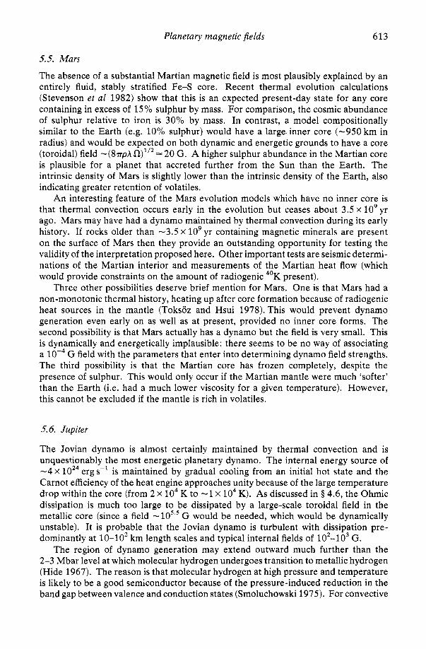
Planetary magnetic fields 613
5.5. Mars
The absence of a substantial Martian magnetic field is most plausibly explained by an entirely fluid, stably stratified Fe-S core. Recent thermal evolution calculations (Stevenson et a1 1982) show that this is an expected present-day state for any core containing in excess of 15% sulphur by mass. For comparison, the cosmic abundance of sulphur relative to iron is 30% by mass. In contrast, a model compositionally similar to the Earth (e.g. 10% sulphur) would have a large. inner core (-950 km in radius) and would be expected on both dynamic and energetic grounds to have a core (toroidal) field -(87rph = 20 G. A higher sulphur abundance in the Martian core is plausible for a planet that accreted further from the Sun than the Earth. The intrinsic density of Mars is slightly lower than the intrinsic density of the Earth, also indicating greater retention of volatiles.
An interesting feature of the Mars evolution models which have no inner core is that thermal convection occurs early in the evolution but ceases about 3.5 x lo9 yr ago. Mars may have had a dynamo maintained by thermal convection during its early history. If rocks older than -3.5 x lo9 yr containing magnetic minerals are present on the surface of Mars then they provide an outstanding opportunity for testing the validity of the interpretation proposed here. Other important tests are seismic determi- nations of the Martian interior and measurements of the Martian heat flow (which would provide constraints on the amount of radiogenic 40K present).
Three other possibilities deserve brief mention for Mars. One is that Mars had a non-monotonic thermal history, heating up after core formation because of radiogenic heat sources in the mantle (Toksoz and Hsui 1978).This would prevent dynamo generation even early on as well as at present, provided no inner core forms. The second possibility is that Mars actually has a dynamo but the field is very small. This is dynamically and energetically implausible: there seems to be no way of associating a lop4 G field with the parameters that enter into determining dynamo field strengths. The third possibility is that the Martian core has frozen completely, despite the presence of sulphur. This would only occur if the Martian mantle were much ‘softer’ than the Earth (i.e. had a much lower viscosity for a given temperature). However, this cannot be excluded if the mantle is rich in volatiles.
5.6. Jupiter
The Jovian dynamo is almost certainly maintained by thermal convection and is unquestionably the most energetic planetary dynamo. The internal energy source of -4 x loz4 erg s-l is maintained by gradual cooling from an initial hot state and the Carnot efficiency of the heat engine approaches unity because of the large temperature drop within the core (from 2 x lo4 K to -1 x lo4 K). As discussed in § 4.6, the Ohmic dissipation is much too large to be dissipated by a large-scale toroidal field in the metallic core (since a field -lo5.’ G would be needed, which would be dynamically unstable). It is probable that the Jovian dynamo is turbulent with dissipation pre- dominantly at 10-102 km length scales and typical internal fields of 102-103 G.
The region of dynamo generation may extend outward much further than the 2-3 Mbar level at which molecular hydrogen undergoes transition to metallic hydrogen (Hide 1967). The reason is that molecular hydrogen at high pressure and temperature is likely to be a good semiconductor because of the pressure-induced reduction in the band gap between valence and conduction states (Smoluchowski 1975). For convective
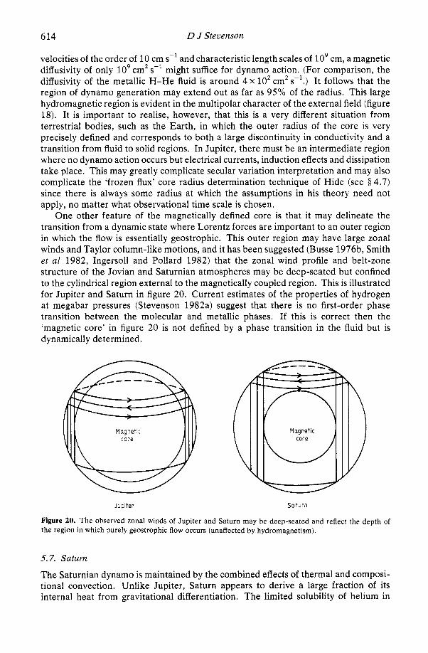
614 D J Stevenson
velocities of the order of 10 cm s-’ and characteristic length scales of 10’ cm, a magnetic diffusivity of only lo9 cmz s-’ might suffice for dynamo action. (For comparison, the diffusivity of the metallic H-He fluid is around 4 x lo2 cm2 s-l.) It follows that the region of dynamo generation may extend out as far as 95% of the radius. This large hydromagnetic region is evident in the multipolar character of the external field (figure 18). It is important to realise, however, that this is a very different situation from terrestrial bodies, such as the Earth, in which the outer radius of the core is very precisely defined and corresponds to both a large discontinuity in conductivity and a transition from fluid to solid regions. In Jupiter, there must be an intermediate region where no dynamo action occurs but electrical currents, induction effects and dissipation take place. This may greatly complicate secular variation interpretation and may also complicate the ‘frozen flux’ core radius determination technique of Hide (see § 4.7) since there is always some radius at which the assumptions in his theory need not apply, no matter what observational time scale is chosen.
One other feature of the magnetically defined core is that it may delineate the transition from a dynamic state where Lorentz forces are important to an outer region in which the flow is essentially geostrophic. This outer region may have large zonal winds and Taylor column-like motions, and it has been suggested (Busse 1976b, Smith et a1 1982, Ingersoll and Pollard 1982) that the zonal wind profile and belt-zone structure of the Jovian and Saturnian atmospheres may be deep-seated but confined to the cylindrical region external to the magnetically coupled region. This is illustrated for Jupiter and Saturn in figure 20. Current estimates of the properties of hydrogen at megabar pressures (Stevenson 1982a) suggest that there is no first-order phase transition between the molecular and metallic phases. If this is correct then the ‘magnetic core’ in figure 20 is not defined by a phase transition in the fluid but is dynamically determined.
Jupiter Saturn
D Figure 20. The observed zonal winds of Jupiter and Saturn may be deep-seated and reflect the depth of the region in which purely geostrophic flow occurs (unaffected by hydromagnetism).
5.7. Saturn
The Saturnian dynamo is maintained by the combined effects of thermal and composi- tional convection. Unlike Jupiter, Saturn appears to derive a large fraction of its internal heat from gravitational differentiation. The limited solubility of helium in
Planetary magnetic fields 615
metallic hydrogen causes helium to rain out into a helium-rich metallic core and provides the layered structure shown in figure 9. The observational evidence to support this structure is the depletion of helium from the atmosphere (relative to Jupiter or to cosmic abundance) and the high heat flow. However, the most interesting consequences of this structure are the alignment and magnitude of the Saturnian magnetic field.
Saturn is very similar to Jupiter in those parameters (rotation rate, magnetic diffusivity, core size and density, heat flow) that determine the dynamo. Consequently, one would expect a very similar magnetic field at the core surface. In fact, there appears to be a significant difference: the dipole field is about 7 G at the 2 Mbar level in Jupiter but only about 1.7 G at the same pressure in Saturn. The alignment of the Saturnian field is its most startling feature: a recent analysis (Connerney et a1 1982b) indicates that the field may be almost exactly spin-axisymmetric. It has been proposed (Stevenson 1980, 1982b) that the explanation for both the low field magnitude and spin axisymmetry involves the helium differentiation and layered structure indicated in figure 9. The idea is that the intermediate, conducting layer between the (almost insulating) helium-depleted molecular envelope and the helium-enriched, uniformly mixed core is incapable of dynamo action because of the stable stratification provided by a helium gradient. However, it undergoes spin-axisymmetric differential rotation because of the thermal winds due to equator-to-pole temperature differences. From the point of view of an external observer, this differential rotation effectively filters out any non-spin-axisymmetric components generated by the dynamo in the core below. The process is essentially equivalent to the electromagnetic skin effect. It has an important observational test: higher-order azimuthal harmonics (m > 1 in the usual spherical harmonic representation) should be more attenuated than m = 1 harmonics.
Despite the smaller region of dynamo generation in Saturn, the energy supply is large ( - loz4 erg s-l) and the Ohmic dissipation is likely to be primarily in small-scale (10-102 km) currents, as in Jupiter. It is likely that large-scale fields are comparable to those in Jupiter (102-103 G).
Detection of secular variation, if possible, would greatly help in testing the interpre- tation given here, since differential rotation should lead to a marked westward or eastward drift, analogous to that detected for the Earth. The ‘frozen flux’ theorem of Hide (1978) may encounter the same difficulty described above for Jupiter but could give an approximate estimate of the outer radius of the inhomogeneous region. This outer radius would also define the external cylindrical region in which deep-seated geostrophic flows occur (Busse 1976b, Smith et a1 1982, Ingersoll and Pollard 1982, figure 20).
5.8. Uranus and Neptune
These planets almost certainly possess dynamos. Interestingly, they each have two physically separated regions in which dynamo action may occur: a liquid iron-rich core which can convect by gradual cooling alone, and a liquid ‘ice’ (H20-NH3, perhaps CH4) layer, the lowermost part of which may be almost metallic and may be convecting. There are three interesting possibilities to consider. If only the iron core provides dynamo action and external field then since its radius is only 15-20’/0 of the planetary radius, the surface field is likely to be only about 0.05 G and should be dominated by the dipole component. It may also be nearly axisymmetric, if differential rotation in a conducting, stably stratified ice layer filters non-spin-axisymmetric components
616 D J Stevenson
(a situation somewhat analogous to Saturn). If dynamo generation occurs in the lowermost part of the ice layer, perhaps out to 40-50% of the planetary radius, then a surface field - 1 G is likely, with higher-order harmonics more prominent and substantial dipole tilt expected. It is intriguing to speculate on a third possibility: interaction between the iron-core dynamo and an ice-layer dynamo: Possibly such a system is more susceptible to fluctuation and reversal than a single dynamo.
5.9. Pluto and giant planet satellites
Large satellites with differentiated structures (figure 8) are likely to possess liquid Fe-S cores. Pluto is structurally and compositionally similar to a large, icy satellite. Since these bodies formed in regions where volatile retention was high, sulphur abundances are likely to approach cosmic abundance, and the cores are then expected to remain completely fluid, because of the very low Fe-S eutectic temperature. As in the terrestrial planets, gradual cooling is not sufficient to sustain core convection. These fluid cores should therefore be stably stratified. It is predicted that all these differentiated satellites have no dynamo-generated magnetic fields. The prediction is actually strongest for Io, the body for which most data exist, because tidal heating is negligible in a fluid core and there is no tendency for the core to cool since heating of the overlying mantle is probably uniform with time (unlike radiogenic heating, which gradually decays).
6. The future
It should be evident that the primary uncertainties in the interpretation of planetary magnetism are of two kinds: incomplete knowledge of the internal dynamic state of the planet, and lack of an adequate predictive dynamo theory. The former problem can only be overcome by additional relevant measurements by spacecraft. Heat flow measurements are needed (especially for the terrestrial planets), seismic data to determine internal structure are essential, detection of magnetic secular variation is desired, and in some cases (especially Mars) the permanent magnetism of surface rocks must be characterised. Most of these necessary observations are not likely to be done in the next twenty years.
Dynamo theory may progress significantly in this time. The major challenge here is to construct a theory which is relevant and applicable. The onset of a planetary dynamo involves a rotation-dominated convective state in which there may be a clear separation of length scales (i.e. a characteristic convective length scale which is much less than the core radius). This problem is amenable to approaches based on mean field hydromagnetics (i.e. the a effect, figure 11) and a semiquantitative approach, as presented here, provides a crude predictive basis for dynamo existence, The major unsolved difficulty here concerns the identification and quantification of sources of differential rotation. (A dynamo can be initiated without differential rotation, but the efficacy of differential rotation is so great that one strongly suspects that it plays an important role.) The finite-field dynamo is much more difficult and theoretically challenging. An outcome of a finite-field theory would be scaling ‘laws’ for the amplitudes of planetary fields. Any expectation of a single, all-encompassing scaling law is probably naive and the testability of scaling laws is questionable, but the existence of (preferably more than one) paradigm for evaluating field amplitudes
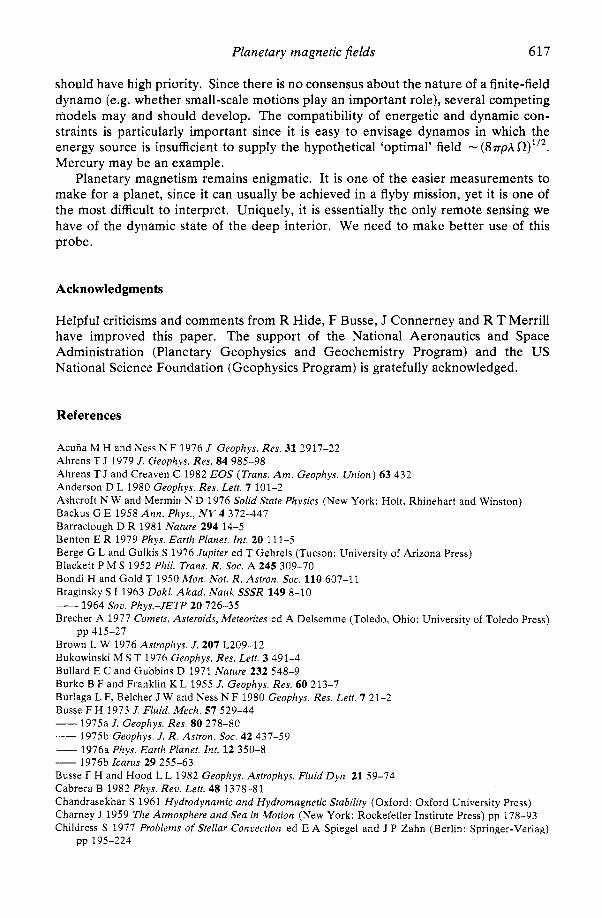
Planetary magnetic fields 617
should have high priority. Since there is no consensus about the nature of a finite-field dynamo (e.g. whether small-scale motions play an important role), several competing models may and should develop. The compatibility of energetic and dynamic con- straints is particularly important since it is easy to envisage dynamos in which the energy source is insufficient to supply the hypothetical ‘optimal’ field - (87rphfl)’”. Mercury may be an example.
Planetary magnetism remains enigmatic. It is one of the easier measurements to make for a planet, since it can usually be achieved in a flyby mission, yet it is one of the most difficult to interpret. Uniquely, it is essentially the only remote sensing we have of the dynamic state of the deep interior. We need to make better use of this probe.
Acknowledgments
Helpful criticisms and comments from R Hide, F Busse, J Connerney and R T Merrill have improved this paper. The support of the National Aeronautics and Space Administration (Planetary Geophysics and Geochemistry Program) and the US National Science Foundation (Geophysics Program) is gratefully acknowledged.
References
Acuria M H and Ness N F 1976 J. Geophys. Res. 31 2917-22 Ahrens T J 1979 J. Geophys. Res. 84 985-98 Ahrens T J and Creaven C 1982 EOS (Trans. Am. Geophys. Union) 63 432 Anderson D L 1980 Geophys. Res. Lett. 7 101-2 Ashcroft N W and Mermiri N D 1976 Solid State Physics (New York: Holt, Rhinehart and Winston) Backus G E 1958 Ann. Phys., N Y 4 372-447 Barraclough D R 1981 Nature 294 14-5 Benton E R 1979 Phys. Earth Planet. Int. 20 111-5 Berge G L and Gulkis S 1976 Jupiter ed T Gehrels (Tucson: University of Arizona Press) Blackett P M S 1952 Phil. Trans. R . Soc. A 245 309-70 Bondi H and Gold T 1950 Mon. Not. R . Asrron. Soc. 110 609-11 Braginsky S I 1963 Dokl. Akad. Nauk SSSR 149 8-10
Brecher A 1977 Comets, Asteroids, Meteorites ed A Delsemme (Toledo, Ohio: University of Toledo Press)
Brown L W 1976 Astrophys. J. 207 L209-12 Bukowinski M S T 1976 Geophys. Res. Lett. 3 491-4 Bullard E C and Gubbins D 1971 Nature 232 548-9 Burke B F and Franklin K L 1955 J. Geophys. Res. 60 213-7 Burlaga L F, Belcher J W and Ness N F 1980 Geophys. Res. Lett. 7 21-2 Busse F H 1973 J. Fluid. Mech. 57 529-44 - 1975a J. Geophys. Res. 80 278-80 - 1975b Geophys. J. R Astron. Soc. 42 437-59 - 1976a Phys. Earrh Planet. Int . 12 350-8 - 1976b karus 29 255-63 Busse F H and Hood L L 1982 Geophys. Astrophys. Fluid Dyn. 21 59-74 Cabrera B 1982 Phys. Rev. Lett. 48 1378-81 Chandrasekhar S 1961 Hydrodynamic and Hydromagnetic Stability (Oxford: Oxford University Press) Charney J 1959 The Atmosphere and Sea in Motion (New York: Rockefeller Institute Press) pp 178-93 Childress S 1977 Problems of Stellar Convection ed E A Spiegel and J P Zahn (Berlin: Springer-Verlag)
- 1964 SOU. Phys.-JETP 20 726-35
pp 415-27
pp 195-224
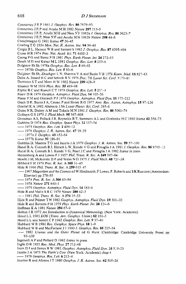
618 D J Stevenson
Connerney J E P 1981 J. Geophys. Res. 86 7679-93. Connerney J E P and Acuiia M H 1982 Nature 297 313-5 Connerney J E P, Acuria M H and Ness 1\7F 1982a J. Geophys. Res. 86 3623-7 Connerney J E P, Ness N F and Acuria M H 1982b Nature 298 44-6 Consolmagno G 1981 Icarus 47 36-45 Cowling T G 1934 Mon. Not. R. Astron. Soc. 94 39-48 Cragin B L, Hanson W B and Santani S 1982 J. Geophys. Res. 87 8395-404 Crane H R 1974 Proc. Nat. Acad. Sci. 7 1 4400-3 Cuong P G and Busse F H 1981 Phys. Earth Planet. Znt. 24 272-83 Desch M D and Kaiser M L 1981 Geophys. Res. Lett. 8 253-6 Dolginov Sh Sh 1978a Geophys. Res. Lett. 5 89-92 - 1978b Geophys. Res. Lett. 5 93-6 Dolginov Sh Sh, Zhuzhgov L N, Sharova V A and Buzin V B 1978 Kosm. Isled. 16 827-63 Duba A, Heard H C and Schock R N 1976 Proc. 7th Lunar Sci. Conf. 3173-81 Durrance S T and Moos H W 1982 Nature 299 428-9 Elsasser W M 1939 Phys. Rev. 55 489-98 Elphic R C and Russell C T 1978 Geophys. Res. Lett. 5 21 1-4 Fearn D R 1979 Geophys. Astrophys. Fluid Dyn. 14 103-26 Flasar F M and Gierasch P J 1978 Geophys. Astrophys. Fluid Dyn. 10 175-212 Gault D E, Burns J A, Cassen P and Strom R G 1977 A n n . Rev. Astron. Astrophys. 15 97-126 Goettel K A 1982 Abstracts 13th Lunar Planet. Sci. Conf. 265-6 Goins N R, Dainty A M and Toksoz M N 1981 J. Geophys. Res. 86 5061-74 Golitsyn G S 1979 J. FluidMech. 95 567-608 Grossman A S, Pollack J B, Reynolds R T, Summers A L and Graboske H C 1980 Icarus 42 358-73 Gubbins D 1974 Rev. Geophys. Space Phys. 12 137-54 - 1975 Geophys. Res. Lett. 2 409-12 - 1976 Geophys. J. R. Astron. Soc. 47 19-39 _. 1977a J . Geophys. 43 453-64 - 1977b Icarus 30 186-91 Gubbins D, Masters T G and Jacobs J A 1979 Geophys. J . R. Astron. Soc. 59 57-100 Hanel R A , Conrath B J, Herath L W, Kunde V G and Pirraglia J A 1981 J. Geophys. Res. 86 8705-12 Hanel R A, Conrath B J, Kunde V G, Pearl J C and Pirraglia J A 1982 Icarus in press Herzenberg A and Lowes F J 1957 Phil. Trans. R. Soc. A 249 507-84 Hewitt J M, McKenzie D P and Weiss N 0 1975 J. Fluid Mech. 68 721-38 Hibberd F H 1979 Proc. R. Soc. A 369 31-45 Hide R 1966 Phil. Trans. R . Soc. A 259 615-47 - 1967 Magnetism and the Cosmos ed W Hindmarsh, F Lowes, P. Roberts and S K Runcorn (Amsterdam:
Elsevier) pp 378-95 - 1974 Proc. R. Soc. A 366 63-84 - 1978 Nature 271 640-1 - 1979 Geophys. Astrophys. Fluid Dyn. 14 183-6 Hide R and Malin S R C 1979 Nature 280 42-3 - 1981 Phil. Trans. R . Soc. A374 15-33 Hide R and Palmer T N 1982 Geophys. Astrophys. Fluid Dyn. 19 301-10 Hide R and Roberts P H 1979 Phys. Earth Planet. Int. 20 124-6 Hoffman K A 1981 Nature 294 67-9 Holton J R 1972 A n Introduction to Dynamical Meteorology (New York: Academic) Hood L L 1981 E O S (Trans. A m . Geophys. Union) 62 161-3 Hood L L and Sonett C P 1982 Geophys. Res. Lett. 9 37-40 Hubbard W B 1980 Rev. Geophys. Space Phys. 18 1-9 Hubbard W B and MacFarlane J J 1980 J. Geophys. Res. 85 225-34 - 1982 Uranus and the Outer Planet ed G Hunt (Cambridge: Cambridge University Press) pp
Ingersoll A P and Pollard D 1982 Icarus in press Inglis D R 1955 Rev. Mod. Phys. 27 212-48 Ivers D J and James R W 1981 Geophys. Astrophys. n u i d Dyn. 16 319-23 Jacobs J A 1975 The Earth’s Core (New York: Academic) chap 4 - 1979 Geophys. Res. Lett. 6 213-4 Jeanloz R and Ahrens J T 1980 Geophys. J . R. Astron. Soc. 62 505-28
93-109
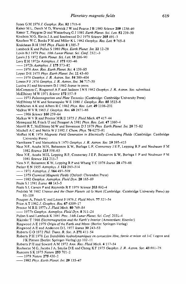
Planetary magnetic fields 619
Jones G M 1976 J. Geophys. Res. 82 1703-9 Kaiser M L, Desch M D, Warwick J W and Pearce J B 1980 Science 209 1238-40 Kaiser T, Piepgras D and Wasserburg G J 1981 Earth Planet. Sci. Lett. 52 239-50 Kivelson M G, Slavin J A and Southwood D J 1979 Science 205 491-3 Knudsen W C, Banks P M and Miller K L 1982 Geophys. Res. Lett. 9 765-8 Kraichnan R H 1965 Phys. Fluids 8 1385-7 Lambeck K and Pullan S 1980 Phys. Earth Planet. Int. 22 12-28 Levin B J 1979 Proc. 10th Lunar Planet. Sci. Conf. 2321-3 Lewis J S 1972 Earth Planet. Sci. Lett. 15 286-90 Levy E H 1972a Astrophys. J . 171 635-46
- 1976 Ann. Rev. Earth Planet. Sci. 4 159-85 Loper D E 1975 Phys. Earth Planet. Int. 11 43-60 - 1978 Geophys. J . R. Astron. Soc. 54 389-404 Lowes F J 1974 Geophys. J. R . Astron. Soc. 36 717-30 Lunine J I and Stevenson D J 1982 Zcarus in press McCammon C, Ringwood A E and Jackson I N S 1982 Geophys. J . R. Astron. Soc. submitted McElhinny M W 1971 Science 172 157-9 - 1973 Paleomagnetism and Plate Tectonics (Cambridge: Cambridge University Press) McElhinny M W and Senanayake W E 1980 J. Geophys. Res. 85 3523-8 McMahan A K and Albers R C 1982 Phys. Rev. Lett. 49 1198-201 Malkus W V R 1963 J. Geophys. Res. 68 2871-86 - 1968 Science 160 259-64 Malkus W V R and Proctor M R E 1975 J. Fluid Mech. 67 417-44 Menequzzi M, Frisch U and Pouquet A 1981 Phys. Rev. Lett. 47 1060-4 Merrill R T, McElhinny M W and Stevenson D J 1979 Phys. Earth Planet. Int. 20 75-82 Mitchell A C and Nellis W J 1982 J. Chem. Phys. 76 6273-81 Moffatt H K 1978 Magnetic Field Generation in Electrically Conducting Fluids (Cambridge: Cambridge
Namikawa T and Matsushita S 1970 Geophys. J . R. Astron. Soc. 19 395-415 Ness N F, Acuiia M H, Behannon K W, Burlaga L F, Connerney J E P, Lepping R P and Neubauer F M
Ness N F, Acutia M H, Lepping R P, Connerney J E P, Behannon K W, Burlaga L F and Neubauer F M
Ness N F, Behannon K W, Lepping R P and Whang Y C 1976 Icarus 28 479-88 Parker E N 1955 Astrophys. J. 122 293-314
- 1979 Cosmical Magnetic Fields (Oxford: Clarendon Press) - 1982 Geophys. Astrophys. Fluid Dyn. 20 165-89 Peale S J 1981 Icarus 48 143-5 Peale S J, Cassen P and Reynolds R T 1979 Science 203 892-4 Podolak M 1982 Uranus and the Outer Planets ed G Hunt (Cambridge: Cambridge University Press) pp
Pouquet A, Frisch U and Lhorat J 1976 J. Fluidhiech. 77 321-54 Price A T 1962 J. Geophys. Res. 67 4309-17 Proctor M R E 1977a J. Fluid Mech. 80 769-84 - 1977b Geophys. Astrophys. Fluid Dyn. 8 311-24 Pullan S and Lambeck K 1981 Proc. 14th Lunar Planet. Sci. Conf. 2031-4 Rikitake T 1966 Electromagnetism and the Earth’s Interior (Amsterdam: Elsevier) Ringwood A E 1979 Origin of the Earth and Moon (Berlin: Springer-Verlag) Ringwood A E and Anderson D L 1977 Icarus 30 243-53 Roberts G 0 1972 Phil. Trans. R. Soc. A 271 411-54 Roberts P H 1978 Les Znstabilitis hydrodynamiques en convection libre, forcie et mixte ed J-C Legros and
J K Platten (Berlin: Springer-Verlag) pp 102-11 Roberts P H and Soward A M 1972 Ann. Rev. Fluid Mech. 4 117-54 Rochester M G, Jacobs J A, Smylie D E and Chong K F 1975 Geophys. J. R. Astron. Soc. 43 661-78 Runcorn S K 1975 Nature 253 701-2 - 1978 Nature 275 430-2 - 1982 Phys. Earth Planet. Int. 29 135-47
- 1972b Astrophys. J. 175 573-81
University Press)
1982 Science 215 558-63
1981 Science 212 211-7
- 1971 Astrophys. J. 164 491-509
93-109
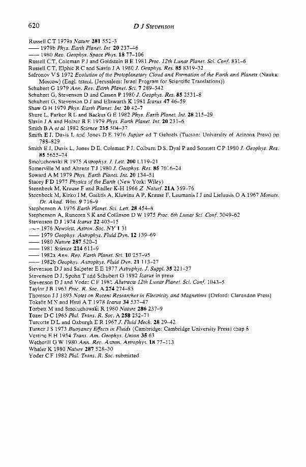
620 D J Stevenson
Russell C T 1979a Nature 281 552-3 - 1979b Phys. Earth Planet. Int. 20 237-46 - 1980 Rev. Geophys. Space Phys. 18 77-106 Russell C T, Coleman P J and Goldstein B E 1981 Proc. 12th Lunar Planet. Sci. Conf. 831-6 Russell C T, Elphic R C and Slavin J A 1980 J. Geophys. Res. 85 8319-32 Safronov V S 1972 Evolution of the Protoplanetary Cloud and Formation of the Earth and Planets (Nauka:
Schubert G 1979 A n n . Rev. Earth Planet. Sci. 7 289-342 Schubert G , Stevenson D and Cassen P 1980 J. Geophys. Res. 85 2531-8 Schubert G, Stevenson D J and Ellsworth K 1981 Icarus 47 46-59 Shaw G H 1979 Phys. Earth Planet. Znt. 20 42-7 Shure L, Parker R L and Backus G E 1982 Phys. Earth Planet. Int. 28 215-29 Slavin J A and Holzer R E 1979 Phys. Earth Planet. Int. 20 231-6 Smith B A et a1 1982 Science 215 504-37 Smith E J, Davis L and Jones D E 1976 Jupiter ed T Gehrels (Tucson: University of Arizona Press) pp
Smith E J, Davis L, Jones D E, Coleman P J, Colburn D S, Dyal P and Sonnett C P 1980 J. Geophys. Res.
Smoluchowski R 1975 Astrophys. J . Lett. 200 L119-21 Somerville M and Ahrens T J 1980 J. Geophys. Res. 85 7016-24 Soward A M 1979 Phys. Earth Planet. Int. 20 134-51 Stacey F D 1977 Physics of the Earth (New York: Wiley) Steenbeck M, Krause F and Radler K-H 1966 Z. Naturf. 21A 369-76 Steenbeck M, Kirko I M, Gailitis A, Klawina A P, Krause F, Laumanis I J and Lielausis 0 A 1967 Monats.
Stephenson A 1976 Earth Planet. Sci. Lett. 28 454-8 Stephenson A, Runcorn S K and Collinson D W 1975 Proc. 6th Lunar Sci. Conf. 3049-62 Stevenson D J 1974 Icarus 22 403-15 - 1976 Newslett. Astron. Soc. NY 1 31 - 1979 Geophys. Astrophys. Fluid Dyn. 12 139-69 - 1980 Nature 287 520-1 - 1981 Science 214 611-9 - 1982a A n n . Rev. Earth Planet. Sci. 10 257-95 - 1982b Geophys. Astrophys. Fluid Dyn. 21 113-27 Stevenson D J and Salpeter E E 1977 Astrophys. J . Suppl. 35 221-37 Stevenson D J, Spohn T and Schubert G 1982 Icarus in press Stevenson D J and Yoder C F 1981 Abstracts 12th Lunar Planet. Sci. Conf. 1043-5 Taylor J B 1963 Proc. R. Soc. A 274 274-83 Thomson J J 1893 Notes on Recent Researches in Electricity and Magnetism (Oxford: Clarendon Press) Toksoz M N and Hsui A T 1978 Zcarus 34 537-47 Torbett M and Smoluchowsci R 1980 Nature 286 237-9 Tozer D C 1965 Phil. Trans. R. Soc. A258 252-71 Turcotte D L and Oxburgh E R 1967 J. Fluid Mech. 28 29-42 Turner J S 1973 Buoyancy Efects in Fluids (Cambridge: Cambridge University Press) chap 8 Vestine E H 1954 Trans. A m . Geophys. Union 35 63 Wetherill G W 1980 A n n . Rev. Astron. Astrophys. 18 77-113 Whaler K 1980 Nature 287 528-30 Yoder C F 1982 Phil. Trans. R. Soc. submitted
Moscow) (Engl. transl. (Jerusalem: Israel Program for Scientific Translations))
788-829
85 5655-74
Dt. A k a d . Wiss. 9 716-9