Plane Magnetic Field Analysis with the Finite

Formulation

Francesco TrevisanDep. of Ingegneria Elettrica, Gestionale e Meccanica, Universita di Udine

Via delle Scienze 208, 33100 Udine, Italy.

e-mail: trevisan@uniud.it, tel.: +39 0432558285, fax: +39 0432558251

December 6, 2002

Abstract: The paper describes the solution of the static and quasi-static bi-dimensional mag-

netic field problems in the framework of the Finite Formulation. The Finite Formulation is a

numerical approach, consisting of an algebraic formulation of the field laws. It adopts the global

variables together with the primal-dual tesselation of the space and time domains. The critical

issue of the derivation of the constitutive equations is also analyzed showing two possible ap-

proaches. Some 2D test problems are discussed in the case of non homogeneus and non linear

media. An axisymmetric eddy current problem has been analysed in addition and the obtained

results have been compared with those from the well established Finite Elements method.

Index Terms: magnetostatic, eddy-currents, Finite Formulation, dual meshes.

1 Introduction

The numerical methods in computational electromagnetism start from a differential approach basedon the Maxwell equations formulated, both in the differential form or in the integral form, in terms ofthe field quantities ρ, J,E,H,B,D. Using a specific discretization method, like the Finite Differences,the Finite Differences in Time Domain [19], the Finite Elements [1], [3], the Edge Elements [4],or the Finite Integration Techniques [18],[9], a set of algebraic equations can be derived to solvenumerically the field equations.

Recently, a relevant theoretical effort has been performed, in order to give a rationale in thenumerical treatment of Maxwell’s equations; the work of Bossavit [6], [5] and the Finite Formulationof Tonti [13] belong to this framework. At the base of both the works, even if not explicitely declaredin the Tonti’s Finite Formulation, are the mathematical tools of the differential forms [7], [21, pp.257-293] and of the algebraic topology [20], [17], used to represent the physical entities of thefields. According to these works the laws of electromagnetism can be restated directly as algebraicequations in a unique way in terms of variables like currents I, voltages U or magnetic fluxes Φ;according to algebraic topology, these variables are cochains which yield real numbers when theyact on chains, and indeed, they can be considered the mathematical abstarctions with the closestmatch to observations we make of the electromagnetic phenomena. To solve the field problems, theconstitutive equations must be also considered, which are a mapping between pointwise objects, thefields or the differential forms used to describe them. This mapping is the Hodge Operator and acrucial issue in computational electromagnetism is to approximate its discrete version, [8]. In FiniteFormulation these mathematical aspects are masked under the hypothesis of the local uniformity ofthe fields.

1

Aim of this paper is to apply and test the Finite Formulation approach tailoring it to the caseof static and quasi- static plane magnetic field analyses in the presence of non homogeneous or nonlinear media. Moreover the crucial point of writing constitutive equations under the hypothesis oflocal uniformity of the fields is analysed in detail showing two possible approaches.

2 Classification of variables

An important issue of the Finite Formulation is a qualitative analysis of the physical variables whichcan be grouped in three main classes: the configuration, the source and the energy variables; thisclassification has been initially introduced in [10], [11] and then revised and improved in [13]. Thisclassification, introduced here for electromagnetic variables, is general and has been applied by Tontito different fields of physics. The configuration variables describe the configuration of the field or ofthe system; examples of the configuration variables are: the electric potential V , the electric voltageU , the electric field vector E, the magnetic flux Φ. The source variables describe the sources of thefield without involving the material parameters; examples of the source variables are: the electriccharge flow Qf , the electric current I, the magnetic voltage F , the magnetic field H. The energyvariables are obtained as the product of a configuration variable by a source variable; examples ofthe energy variables are: the work, the magnetic energy density, the Poynting vector.

The link between fields (pointwise objects) belonging to the class of configuration or sourcevariables respectively, are the constitutive equations that contain the material properties and themetric notions such as lengths, areas and volumes; in this paper, the magnetic constitutive equationand the Ohm’s law will be examined in detail.

The Finite Formulation makes also use of the so called global variables that formally are p-cochains, [17]. The global variables are associated with oriented space and time elements like pointsP, lines L, surfaces S, volumes V, time instants I and time intervals T (the bold face evidence thatthe elements are oriented). The global variables, relevant to our static or quasi-static magnetic fieldanalysis are: the electric potential impulse V, the electric voltage impulse U , the magnetic flux Φ,the circulation p of the magnetic vector potential, the electric charge flow Qf , the magnetic voltageimpulse F . These global variables are reported in Table 1 divided into configuration and sourcevariables.

Table 1: Global variables of interest in magnetostatic and magneto quasi-static andtheir relation with the field functions

configurationglobal variables [Wb]

V =∫T

V dt U =∫TL

E · dL dt Φ =∫S

B · dS p =∫L

A · dL

sourceglobal variables [C]

Qf =∫TS

J · dSdt F =∫TL

H · dLdt

Global variables are related to the fields (electric potential V , electric field E, magnetic inductionB, magnetic vector potential A, current density J, magnetic field H respectively) by means of anintegration performed on lines L, surfaces S, and time intervals T; a tilde on the integration domainsT, S is used to distinguish one of the two possible orientations of the geometric elements, as will beexplained later.

2.1 Orientation of the geometrical elements

Space P, L, S, V and time elements I, T need to be oriented in order to define the sign of theassociated global variables. There are two kinds of orientations: inner and outer. Moreover the

2

notion of outer orientation depends on the dimension of the embedding space.If we consider the 3D space, the inner orientation can be defined as follows: the points P can be

oriented as sinks, the lines L are oriented by a direction chosen on them, the surfaces S are endowedwith inner orientation when their boundary line (∂S) has an inner orientation and the volumes Vare endowed with inner orientation when their boundary surface (∂V) has inner orientation.

On the other hand the outer orientation of a volume V is based on the choice of outward (orinward) normals on its boundary. For a surface S the outer orientation is defined when we fixan arrow crossing the surface from the negative to the positive face: it is equivalent to the innerorientation of the line L crossing the surface. A line L is endowed with outer orientation when adirection of rotation around the line has been defined: it is equivalent to the inner orientation of asurface S crossing the line. The outer orientation of a point P can be defined as the inner orientationof the volume V enclosing the point.

In the case of the time axis, the embedding space is 1 D; therefore a primal instant I is endowedwith inner orientation when its point on the time axis is oriented as a sink; a primal interval T hasthe inner orientation when it is oriented toward increasing time. The outer orientation of a dualinstant I is the inner orientation of the primal interval to which it belongs. The outer orientation ofa dual interval T is the inner orientation of the primal instant internal to it.

2.2 Discretisation of space and time in cell complexes

Instead of considering all the possible oriented geometric elements, a discretisation of space and timeis now introduced.

Nodes pk, edges lj , faces si and cells vh form a cell complex G and are representative of points P,lines L, surfaces S and volumes V respectively; the subscripts are required to number the geometricalelements. Once we have defined a cell complex, called primal complex , we can introduce an othercell complex called dual complex G made of geometrical elements denoted by ph, li, sj , vk with atilde to distinguish them from the corresponding geometrical elements of the primal cell complex G.The duality between the two complexes G and G assures that the geometrical elements correspondas follows: pk ↔ vk, lj ↔ sj , si ↔ li,vh ↔ ph.

The primal cell complex considered here is based on Delaunay triangles. Different choices ofthe point, inside each primal cell vh, to be chosen as dual point ph of the dual cell complex, arepossible. In this paper the barycenters of the primal cells are selected as ph and therefore a dualedge li connects the barycenters of two adjacent primal cells via the barycenter of the common facesi, Fig. 1; this is the barycentric subdivision. The G-G barycentric cell complexes are easy to begenerated and can be straightforwardly extended to the 3D geometries.

In the plane field problems, primal cells are prisms with unit thickness (or unit angular width inthe axisymmetric fields) and triangular base; the dual edges are broken lines crossing the primal facesat their barycenter. Dual cells are prisms with unit thickness (or unit angular width in axisymmetricfields) and are staggered respect to the primal cells.

We assume to assign to all the elements of a primal complex G the inner orientation. If a cellcomplex G has been endowed with inner orientation, the outer orientation is induced on the spaceelements of its dual complex G and therefore all the dual elements are automatically endowed withouter orientation.

We indicate with Nv the number of primal cells vh, with Ns the number of primal faces si (dueto the plane symmetry the top-bottom faces of the prisms are omitted in the count), with Nl thenumber of primal edges lj (the edges normal to the plane of symmetry are neglected in the count),and with Np the number of primal nodes pk (only the three vertices of the top triangle of eachprimal cell are accounted for).

In the case of the dual cell complex G the duality assures that the following equalities hold:Nv = Np, Ns = Nl, Nl = Ns and Np = Nv.

3

AAAAAAAAAAAAAAAAAAAAAAAA

AAA

AAA

AAAAAAAA

AAAAAAAAA

AAAAAAAAAAAA

AAAAAA

AAAAAAAAA AA

AAAAAAAAA

li

sj

vk

~

~

~

dual cell

primal cell

pk

vh

si

lj

ph~

li~

lj

pk

ph~

Figure 1: Detail of a simplicial primal-dual barycentric cell complex for plane or axisymmetricfield problems. Inner and outer orientations of a primal and dual line and of a primal and dualface are shown.

nT

t n+ 1

time

nT

n+1T

t n

n+1T

tn-1 t tn n+1

~ ~

~~

Figure 2: primal - dual discretisation of the time axis.

4

A primal cell complex is introduced on the time axis also. Its elements are the primal instantst1, t2 ,..., tn and the primal intervals T1, T2 ,..., Tn with inner orientation. The dual complex hasdual instants t1, t2, ..., tn and dual intervals T1, T2, ..., Tn , Fig. 2, endowed with outer orientationthat is the inner orientation of the primal complex.

2.3 Global variables and cell complexes

As a result of Tonti’s Finite Formulation [15], [16], there is a coupling between global variablesand oriented space and time geometrical elements of a cell complex, such that: the configurationvariables can be associated with space and time elements endowed with inner orientation and so tothe primal cell complexes, while the source variables can be associated with space and time elementsendowed with outer orientation and so to dual cell complexes. This association of global variablesto oriented space and time geometrical elements, plays a key role to provide a discrete formulationof laws in many theories of physics and it is useful in computational electromagnetism; in the caseof the magnetostatic and magneto quasi-static field, the association above can be summarised asfollows:

• the electric potential impulse V[Tn,pk] is relative to primal intervals Tn and to primal nodespk;

• the electric voltage impulse U [Tn, lj ] is relative to the primal intervals Tn and to the primaledges lj ;

• the magnetic flux Φ[tn, si] is relative to the primal instants tn and primal faces si;

• the circulation p[tn, lj ] of the magnetic vector potential is relative to the primal instants tn

and to the primal edges lj ;

• the electric charge flow Qf [Tn, sj ] is relative to dual intervals Tn and to dual faces sj ;

• the magnetic voltage impulse F [Tn, li] is relative to dual intervals Tn and to dual edges li.

3 Magnetostatic and magneto quasi-static laws in finite form

In the following, the laws relevant for magnetostatic and magneto quasi-static field analysis will beapplied to the corresponding geometrical elements of the above defined cell complexes in space andtime; so doing, the corresponding algebraic equations will be derived. These algebraic equations linkconfiguration variables with configuration variables and source variables with source variables andare valid in whatever medium. They do not involve metric notions, i.e. lengths, areas, measures ofvolumes and durations and they are valid both in the large and in the small , [7], [13].

3.1 Gauss magnetic law

Considering the primal cells vh and the primal faces si, Fig. 3, the Gauss magnetic law, with matrixnotation, becomes:

D Φ = 0 (1)

where D is the incidence matrix D = ||dhi|| of dimension NvxNs between the inner orientations ofvh and si; Φ = [Φ1,Φ2, ...ΦNs ]

T is the vector of fluxes of dimension Ns. Due to the plane symmetry,only the lateral faces of the volume vh have to be considered in (1). The flux Φi relative to a primal

5

vh

la

si

lb

~

lj

l1

~l7

~l6

~l5

~l4~

l3

~l2

~sj

s2s1

s3

Figure 3: A primal volume vh and the corresponding primal faces exploded with the inner orien-tation for the case of a plane field; with these orientations Φ1 +Φ2 −Φ3 = 0. For a lateral primalface si with primal edges la, lb normal to the plane of symmetry Φi = pb − pa.On the right a dualface sj (top or bottom of vk) and its boundary of dual edges li with outer orientation; with theseorientations F1 −F2 −F3 −F4 + F5 + F6 −F7 = Qf

i.

face si, can be expressed as the circulation p of the magnetic vector potential along the boundaryedges of the face si:

Φi =4∑

j=1

cij p[tn, lj ] (2)

cij are the incidence numbers between the inner orientation of the primal edge lj and the innerorientation of the corresponding primal face si. Due to the plane symmetry, only the boundaryprimal edges of si normal to the plane of symmetry contribute in (2). Introducing the vector ofthe circulations p = [p1, p2, ..., pNp ]T along the primal edges lj normal to the plane of symmetry, ofdimension Np, (2) becomes:

Φ = C p (3)

being C = ||cij || the incidence matrix, of dimension NsxNp; (3) identically satisfies (1) being D C ≡ 0.

3.2 Ampere’s law

Assuming here a charge flow normal to the plane of symmetry, the Qf crossing the lateral dual facesof vk is null. Therefore, considering the dual faces sj laying on the symmetry plane, Fig. 3 right,the Ampere law can be written as:

CF = Qf (4)

being C = ||cji|| the incidence matrix, of dimension NsxNl, between the outer orientations of vk

and li; F = [F1,F2, ...,FNs]T is the vector of the magnetic voltage impulses of dimension Ns and

Qf = [Qf1, Q

f2, ..., Q

fNs

]T is the vector of electric charge flows.Note that the continuity equation for static and quasi-static fields is identically satisfied with a

charge flow normal to the plane of symmetry and therefore it will not be considered.

3.3 Faraday-Neumann law

Considering the primal faces si, Fig. 3 center, with two boundary edges la, lb normal to the symmetryplane, the Faraday-Neumann law can be written as:

4∑i=1

cij U [Tn+1, lj ] = Φ[tn, si] − Φ[tn+1, si] (5)

6

where cij are the incidence numbers between the inner orientation of the edges lj forming theboundary of si and the inner orientation of si. Due to the plane symmetry, only the electric voltageimpulses along the edges la, lb contribute in (5). With matrix notation (5) can be rewritten as:

CU[Tn+1] = Φ(tn) − Φ(tn+1) (6)

being C = ||cij || the incidence matrix, of dimension NsxNp, Np is the number of primal nodes equalto the number of primal lines normal to the symmetry plane; U = [U1,U2, ...,UNp ]T is the vectorelectric voltage impulses of dimension Np, relative to the primal edges lp normal to the plane ofsymmetry. Substituting (3) in (6), the Faraday-Neumann law, rewritten in terms of the circulationof the magnetic vector potential, becomes:

U[Tn+1] = p(tn) − p(tn+1) (7)

The plane symmetry assure that the electric scalar potential impulse V at the two points, formingthe boundary of lp, are identical; therefore their difference do not contribute to the electric voltageimpulse U [Tn+1, lp].

3.4 Rates of global variables

It is convenient to introduce the temporal rates of global variables associated with a time intervallike U , F , Qf . If these global variables are approximated to depend linearly on the duration of asufficiently small interval, then the mean rate approximates the value of the instantaneus rate at themiddle instant of the interval, Fig. 2. Therefore the rates of U , F , Qf are the electric voltage, themagnetic voltage and the electric current respectively and are computed as:

Uj(tn) ≈ U [Tn, lj ]Tn

, Fi(tn) ≈ F [Tn, li]Tn

, Ij(tn) ≈ Qf [Tn, sj ]Tn

(8)

Uj(tn), Fi(tn) and Ij(tn) are functions of time instants and their association with lj , li and sj

respectively, is accounted for with a subscript index.Therefore the Ampere’s law (4) and the Faraday-Neumann law (7) can be respectively rewritten

as:C F(tn) = I(tn) (9)

U(tn+1) =p(tn) − p(tn+1)

Tn+1(10)

in terms of the electric voltage vector U = [U1, U2, ..., UNP]T, the magnetic voltage vector F =

[F1, F2, ..., FNl]T and the electric current vector I = [I1, I2, ..., INs

]T.

4 Constitutive equations

The constitutive equations, link the field source variables with the field configuration variables.These equations contain the material parameters and require metric notions such as length andareas. Fields are unavoidably needed to introduce the constitutive laws and the assumption is theuniformity of fields within a triangle or within its subregions.

4.1 Magnetic constitutive equation

The first step in the construction of the magnetic constitutive equation for triangular primal andbarycentric dual cells is to work locally element by element and then assemble globally each localmaterial equation. With reference to Fig. 4, an oriented primal cell (a triangle) is considered with

7

primal nodes a, b, c, primal edges l1, l2, l3 and primal faces s1, s2, s3 with inner orientation andlocal numbering; l1, l2, l3 are the corresponding portions of dual edges with outer orientation, againwith local numbering. It should be noted that the primal faces and the corresponding portions of

a b

c

l2

a b

c

l1

l3

s1

~l1

s3

~l3

~l3

~l1

~l2

~l2

l2 l

1

l3

s2

Figure 4: Primal cell and a portion of the dual cell with outer orientation; on the right the 2Dcorresponding primal cell and portions of the dual edges.

dual edges are not orthogonal as in the Delaunay-Voronoy tesselation.The magnetic material is assumed homogeneous inside each primal cell, characterised by the

following permeability matrix:

µ =[µ1,1 µ1,2

µ2,1 µ2,2

](11)

where the numbers µij can be constants or functions of the element flux density in the non-linearcase. In the following two possible approaches are described to derive the local constitutive matrixbetween the vector of magnetic voltages Fe = [F1, F2, F3]T and the flux vector Φe = [Φ1, Φ2, Φ3]T

both related to an element e. A first approach assumes three subregions with uniform fields, [22]; itcan be extended to quadrilateral primal cells. A second approach assumes the uniformity of fields onthe whole triangle; it implies a sensible simplification but it is applicable to simplexes only. Becauseof Gauss’s law, in the case of triangles, the uniformity in subregions implies the uniformity in thewhole triangle but it is not true for quadrilateral elements.

4.1.1 Uniformity subregions

It is convenient to introduce for each element an influence region around each vertex a, b, c delimitedby a couple of portions of dual edges. In each influence region a, b, c the magnetic field Ha, Hb, Hc

and the flux density Ba, Bb, Bc vectors, are assumed uniform; each vector has two components (x,y) or (r, z) depending on the 2D problem (plane or axisymmetric).

The three magnetic voltages F1, F2, F3 along the three portions of dual edges l1, l2, l3 respectivelycan be expressed as in Table 2:

Table 2: Magnetic voltages

Region a Region b Region c[F2

F3

]=

[l2l3

]Ha = La Ha

[F1

F3

]=

[l1l3

]Hb = Lb Hb

[F1

F2

]=

[l1l2

]Hc = Lc Hc

where l1, l2, l3 are row vectors, of dimension 2, with direction of the portion of dual edge andorientation induced by the right-screw rule from the outer orientation of the dual edge itself. Thecontinuity of the tangential components of the magnetic field is so automatically satisfied.

8

La, Lb, Lc are 2x2 non singular matrices that can be inverted and the corresponding inverse can bemodified by introducing a column of zeros as follows:

Aa =[

0 x x0 x x

]Ab =

[x 0 xx 0 x

]Ac =

[x x 0x x 0

](12)

where x indicates a non null element. Therefore the magnetic fields Ha, Hb, Hc in each influenceregion, can be deduced from the local vector of magnetic voltages Fe as:

Ha = Aa Fe, Hb = Ab Fe, Hc = Ac Fe (13)

Due to the plane symmetry of the field, only the fluxes Φ1, Φ2, Φ3 relative to the primal lateral

a b

c

s2

s1

s3

a b

c

s1

s2

s3

Φ3a

Φ3b

Φ2a

Φ2c

Φ1c

Φ1b

Φ3a

Φ3b

Φ1c

Φ1b

Φ2a

Φ2c

Figure 5: Primal cell with the area vectors normal to the primal faces s1, s2, s3; the orientationof the vectors derives from the inner orientation of the respective face using the right-screw rule.

faces s1, s2, s3 need to be considered, Fig. 5. From the flux densities Ba, Bb, Bc in each region ofinfluence a, b, c and using the addittivity of the flux on portions of the primal faces, the fluxes canbe expressed as:

Φ1 = Φ1b + Φ1c = 1

2 s1 Bb + 12 s1 Bc

Φ2 = Φ2a + Φ2c = 12 s2 Ba + 1

2 s2 Bc

Φ3 = Φ3a + Φ3b = 12 s3 Ba + 1

2 s3 Bb

(14)

being s1, s2, s3 the area row vectors, of dimension 2, normal to the primal faces s1, s2, s3; theorientation of s1, s2, s3 is congruent with the inner orientation of the corresponding face accordingto the right-screw rule. The additivity of the fluxes automatically assures the continuity of thenormal components of the induction at the primal faces.

Now from the constitutive equation linking the fields:

Bj = µHj , j = a, b, c (15)

inside each influence region of a primal cell, the local constitutive equation in terms of the globalvariables can be derived by substituting in (14), the expressions (15) and (13), obtaining:

Φ1 =12

s1 µ (Ab + Ac) Fe, Φ2 =12

s2 µ (Aa + Ac)Fe, Φ3 =12

s3 µ (Aa + Ab)Fe (16)

From the local flux vector Φe, (16) becomes:

Φe = MeF Fe (17)

where the 3x3 local matrix MeF is defined as:

MeF =

12

s1 µ (Ab + Ac)

s2 µ (Aa + Ac)s3 µ (Aa + Ab)

(18)

9

In the numerical formulation for magnetostatic and magneto quasi-static presented here, the inverseMe

Φ of the matrix MeF need to be considered, such that:

Fe = MeΦ Φe (19)

Note that the local matrix MeΦ is not symmetric, due to the choice of a primal-dual barycentric cell

complex; moreover it is non singular and its eigenvalues are all positive. On the other hand, in thecase of a Delaunay-Voronoi cell complex the matrix Me

Φ becomes diagonal.

4.1.2 Uniformity on the whole triangle

From the three fluxes and the area row vectors s1, s2, s3, the uniform field B in the whole trianglecan be derived as:

B =[

s2s3

]−1 [Φ2

Φ3

]=

[s1s3

]−1 [Φ1

Φ3

]=

[s1s2

]−1 [Φ1

Φ2

](20)

In terms of the local flux vector Φe, (20) can be rewritten as:

B = WaΦe = WbΦe = WcΦe (21)

where the 2 × 3 matrices Wj with j = a, b, c, correspond to the matrices in (20) with in addition acolum of zeros in correspondence of the missing flux. Such a uniform field B identically satisfies theGauss law (1). From the inverse of (15) the uniform magnetic field is obtained and then projectingH along the portion of the dual edge opposite to the node a, b, c in turn, the vector of the magneticvoltages Fe can be derived as:

Fe =

l1 ν Wa

l2 ν Wb

l3 ν Wc

Φe = Me′

ΦΦe (22)

where ν is the 3×3 reluctivity matrix and Me′Φ is the non singular non symmetric constitutive matrix

having null diagonal elements. Me′Φ has two over three eigenvalues λi > 0, λj > 0 and coincident

with those of MeΦ in (19); being the trace(Me′

Φ) = 0 the third eigenvalue is −λi − λj .A different constitutive matrix can be deduced from the three matrices Wj in (21) by expressing

the magnetic field as H = 13ν(Wa +Wb +Wc); therefore projecting it along the potions of dual edges

we have:

Fe =13

l1

l2l3

ν(Wa + Wb + Wc)Φe = Me′′

ΦΦe (23)

where the constitutive matrix Me′′Φ is now singular with rank 2 but the two non null eigenvalues are

coincident with λi, λj .

4.1.3 Constitutive matrix in terms of p

The local flux vector Φe can be expressed in terms of the local vector pe = [p1, p2, p3]T of thecirculations of the magnetic vector potential as in (2), and with matrix notation it becomes:

Φe = Ce pe (24)

Ce is the local incidence matrix between the inner orientation of the primal edges lp, normal to theplane of symmetry, and the inner orientation of the corresponding primal face si. Substituting (24)in (19) or in (22) or in (23) the following local constitutive equation is derived:

Fe = MeΦ Ce pe = Me′

Φ Ce pe = Me′′Φ Ce pe (25)

10

where it can be proved that the matrices MeΦ Ce ≡ Me′

Φ Ce ≡ Me′′Φ Ce are coincident even though

MeΦ, Me′

Φ and Me′′Φ are not; due to this fact the two approaches for the contitutive equations are

equivalent.In terms of the global vector p(tn) of the circulations of the magnetic vector potential relative

to the primal edges lp normal to the plane of symmetry, the global constitutive equation can beassembled element by element from (25):

F(tn) = MΦ C p(tn) (26)

being C = ||cij || the incindence matrix and MΦ C the global constitutive matrix of dimensionNs×Nlp .

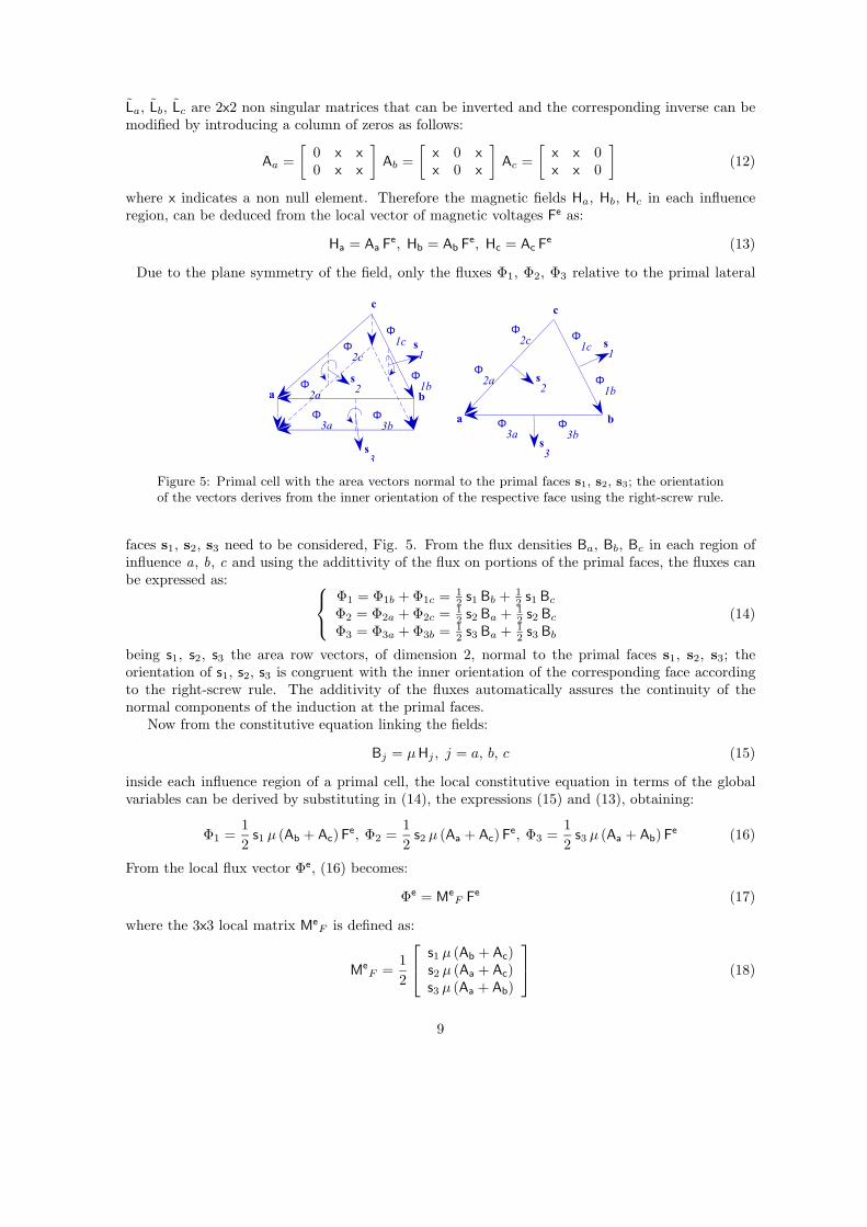
4.2 Ohm’s constitutive equation

In the case of magneto-quasistatic field analysis, the Ohm’s law is required for the conductive regions.For plane (or axisymmetric) problems with electric current normal to the plane of symmetry, theOhm’s law is relative to a dual face sP laying on the plane of symmetry, and to the primal line lPnormal to that plane, crossing sP , Fig. 6. The Ohm’s law, written locally for a primal element e,

AAAAAAAAAAAAAAAAAAAAAAAAAAAAAA

sP

~

lP

AAAAAAAAAAAAAAAAAAAAAAAAAAAAAAAAAAAAAAAAAAAAAAAAA

sp

~

p

a b

c

AAAAAAAAAAAAs

a

~sc~

sb

~

la

lb

lc

Figure 6: Dual cell sP (left) and a cluster of primal elements with the common primal edge lPnormal to the plane of symmetry; the generic primal element of the cluster is evidenced on theright with local numbering (a, b, c) of the nodes and of the portions of dual areas internal to it.

with primal nodes a,b, c primal edges la, lb, lc normal to the plane of symmetry, can be written as:

12[Ii(tn) + Ii(tn+1)] = σe si

li[Ui(tn+1) + Ui

ext(tn+1)], with i = a, b, c (27)

where σe is the uniform conductivity of the element and Uiext(tn+1) is the external impressed voltage

relative to a primal line li, with i = a, b, c; in the case of a passive conductor Uiext(tn+1) ≡ 0.

Ia, Ib, Ic are fractions of the currents, relative to the portions of dual faces sa, sb, sc, tailored insidethe triangular primal element e. Being the dual mesh barycentric, the following identity holds:

sa ≡ sb ≡ sc =se

3(28)

where se is the area of the triangle e.Note that, in (27), the voltages and the currents refer to different temporal grids, Fig. 2, staggered

one respect to the other. The assumption that Qf depends linearly on the dual interval duration,

11

assures that the current is relative to the mid instant of the dual interval corresponding to the primalinstant. Therefore the quantity 1

2 [Ii(tn)+ Ii(tn+1)] is referred to the intermediate dual instant tn+1.Assembling the local equation (27) for each primal element e of the cluster of elements having

the common primal edge lP , the global constitutive Ohm’s law can be derived as:

I(tn) + I(tn+1) = 2G [U(tn+1) + Uext(tn+1)] (29)

being G the NscxNsc diagonal matrix relative to the conductor nodes.

5 Solution of the magnetostatic problem

The algebraic system for the solution of the plane magnetostatic field analysis, can be derived bysubstituting in the Ampere equation (9) the magnetic constitutive equation (26) where the fluxvector is expressed in terms of the circulation of the vector potential vector p relative to the edgeslP (individuated by the NP nodes of the 2D mesh) normal to the plane of symmetry assumed hereof unit length. The resulting system of order NP, formally becomes:

C MΦ C p = I (30)

where due to the duality of the complexes C = CT; in the implementation the incidence matrix Cneeds not to be computed or stored and the stiffness matrix in (30) can be easily assembled workingelement by element. An important proprety of the stiffness matrix C MΦ C can be proved: it issymmetric even thougth the constitutive matrix MΦ is not; C MΦ C is sparse having, for each row,a number of non null elements equal to the number of triangles forming a cluster with a node incommon.

To solve (30) the boundary conditions have to be considered in addition, assigning p at theboundary nodes. Moreover symmetry conditions, like ”flux parallel” or ”flux normal” can be easilyhandled by imposing respectively a null value of the circulations or a leaving unknown the corre-sponding circulation values relative to the nodes of the symmetry line.

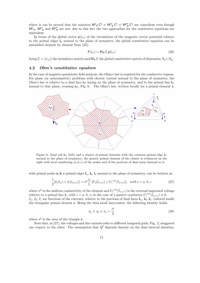
5.1 Numerical results in magnetostatic problems

In Fig. 7 a circle of radius R = 1 m of relative permeability µr = 1000, surrounded by air with anexternal impressed field B0 = 1 T is considered. Due to the symmetry only one half of the mesh isconsidered and a linear pb per unit depth has been imposed on the boundary nodes of the left, topand right boundary. the number of triangles is 4141 and the number of nodes 2108. The analyticalvalue of the field within the circle is B = 2B0(µr − 1)/(µr + 2) = 1.9940 while the computed valueaveraged among the elements of the circle is Bc = 1.9519.

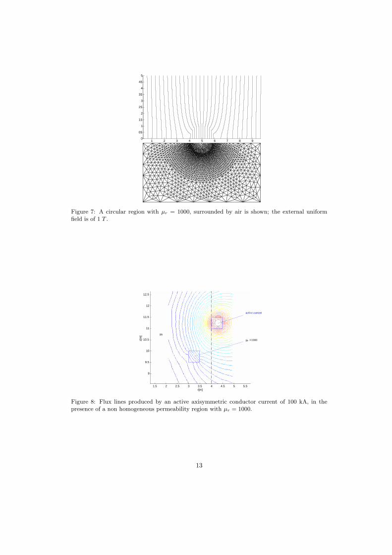
Fig. 8 shows the flux lines produced by an axisymmetric current of 100 kA uniformly distributedin an active conductor, in presence of a non homogeneous media, an axisymmetric square regionwith relative permeability µr = 1000 surrounded by air.

Due to the axisymmetry of the problem, the vector ψ of the circulations of the vector potentialfor radian has been introduced:

ψ =p

α(31)

relative to the primal nodes of the 2D mesh, being α the azimuthal angular width of the cellcomplexes in φ direction in a (r, φ, z) cylindrical reference frame.

The boundary conditions considered here are ψb ≡ 0, at the boundary primal nodes Pb of themesh.

In the presence of a non linear media the system (30) has been iteratively solved by means of aquasi-Newton method, the Broyden method [12] with a numerical estimate of the Hessian matrix

12

1 2 3 4 5 6 7 8 90

0.5

1

1.5

2

2.5

3

3.5

4

4.5

5

Figure 7: A circular region with µr = 1000, surrounded by air is shown; the external uniformfield is of 1 T .

AAAAAAAAAAAAAAA

AAAAAAAAAAAAAAA

AAAAAAAAAAAAAAA

AAAAAAAAAAAAAAA

AAAAAAAAAAAAAAA

AAAAAAAAAAAAAAA

AAAAAAAAAAAAAAA

AAAAAAAAAAAAAAA

AAAAAAAAAAAAAAA

AAAAAAAAAAAAAAAAAAAAAAAAAAAAAA

AAAAAAAAAAAAAAA

AAAAAAAAAAAAAAAAAAAAAAAAAAAAAAAAAAAAAAAAAAAAAAAAAAAAAAAAAAAA

AAAAAAAAAAAAAAA

1.5 2 2.5 3 3.5 4 4.5 5 5.5

9

9.5

10

10.5

11

11.5

12

12.5

r[m]

z[m

]

active current

µr =1000

µ0

Figure 8: Flux lines produced by an active axisymmetric conductor current of 100 kA, in thepresence of a non homogeneous permeability region with µr = 1000.

13

kept constant during the iterations. As initial guess of the iteration process, the flux distribution,computed from the homogeneous media, has been considered. The stop criterium considered isthe relative discrepancy of the flux distribution in the ferromagnetic region, between two successiveiterations. At each iteration the induction field, uniform within each triangle, has been computedfrom the circulations of the vector potential according to (24) and (21). Fig. 9 shows the resulting fluxlines when the non-linear media characteristic, reported in Fig. 10, is assumed for the ferromagneticregion and the active coil is fed with a 100 kA axisymmetric uniform current.

6 Solution of the magneto quasi-static problem

To illustrate the numerical formulation for the solution of a magneto quasi-static field problem, asimple linear axisymmetric Eddy Current Problem (ECP) has been considered: a massive activeconductor, of known conductivity is fed with a known external time dependent voltage source inpresence of a closed passive massive coil. All the materials are here assumed homogeneous andlinear, even though the extension to non homogeneous or non linear media is straightforward. Dueto the axisymmetry of the ECP, the resulting eddy currents are all azimuthal (along φ direction),Fig. 11. With respect to the cell complexes shown in Fig. 11, the vector of the electric voltagesper radian can be introduced:

u(tn+1) =U(tn+1)α

(32)

referred to the primal nodes P that are the nodes of the primal 2D mesh, corresponding to the firstnodes of the primal edges in the azimuthal direction (e. g. li, lj , lk in Fig. 11); α is the azimuthalangular width of the cell complexes.

Substituting (32) in the Faraday-Neumann equation (10) the circulation per radian ψ (31), itbecomes:

u(tn+1) =ψ(tn) −ψ(tn+1)

Tn+1(33)

6.1 The iterative numerical method

The linear algebraic system to be solved, consists of two sets of equations.

1. Equations relative to the air nodes

In the air primal nodes the homogeneous equation, deduced from (30), holds:

C MΦ Cψ = 0 (34)

2. Equations relative to the conductor nodes

Substituting in the Ohm’s constitutive equation (29) the vector of current’s given by (30)written for two successive primal time instants tn and tn+1 and the vector of the electricvoltages for radian for (33), the following equations can be derived for the conductor nodes:

(CTMΦ C +2

Tn+1G∗)ψ(tn+1) = −(CTMΦ C − 2

Tn+1G∗)ψ(tn) + 2G∗ uext(tn+1) (35)

where G∗ = G/α indicates the diagonal matrix of conductances for radian.

Combining the above two sets of equations 1 and 2, the following implicit numerical scheme can bederived:

Pψ(tn+1) = Qψ(tn) + q(tn+1) (36)

being P and Q, NPxNP matrices whose elements are those of:

14

AAAAAAAAAAAAAA

AAAAAAAAAAAAAA

AAAAAAAAAAAAAA

AAAAAAAAAAAAAA

AAAAAAAAAAAAAA

AAAAAAAAAAAAAA

AAAAAAAAAAAAAA

AAAAAAAAAAAAAA

AAAAAAAAAAAAAAAA

AAAAAAAAAAAAAAAAAAAAAAAAAAAAAAAA

AAAAAAAAAAAAAAAA

AAAAAAAAAAAAAAAAAAAAAAAAAAAAAAAA

AAAAAAAAAAAAAAAA

AAAAAAAAAAAAAAAA

1.5 2 2.5 3 3.5 4 4.5 5 5.5

9

9.5

10

10.5

11

11.5

12

12.5

r[m]

z[m

]

initial guess

AAAAAAAAAAAAAA

AAAAAAAAAAAAAA

AAAAAAAAAAAAAA

AAAAAAAAAAAAAA

AAAAAAAAAAAAAA

AAAAAAAAAAAAAA

AAAAAAAAAAAAAA

AAAAAAAAAAAAAAAAAAAAAAAAAAAA

AAAAAAAAAAAAAA

AAAAAAAAAAAAAAAA

AAAAAAAAAAAAAAAAAAAAAAAAAAAAAAAA

AAAAAAAAAAAAAAAA

AAAAAAAAAAAAAAAAAAAAAAAAAAAAAAAA

AAAAAAAAAAAAAAAA

AAAAAAAAAAAAAAAA

1.5 2 2.5 3 3.5 4 4.5 5 5.5

9

9.5

10

10.5

11

11.5

12

12.5

r[m]

z[m

]

second iteration

AAAAAAAAAAAAAA

AAAAAAAAAAAAAA

AAAAAAAAAAAAAA

AAAAAAAAAAAAAA

AAAAAAAAAAAAAA

AAAAAAAAAAAAAA

AAAAAAAAAAAAAA

AAAAAAAAAAAAAA

AAAAAAAAAAAAAA

AAAAAAAAAAAAAAA

AAAAAAAAAAAAAAAAAAAAAAAAAAAAAA

AAAAAAAAAAAAAAA

AAAAAAAAAAAAAAAAAAAAAAAAAAAAAA

AAAAAAAAAAAAAAA

AAAAAAAAAAAAAAA

1.5 2 2.5 3 3.5 4 4.5 5 5.5

9

9.5

10

10.5

11

11.5

12

12.5

r[m]

z[m

]

8-th iteration

Figure 9: Flux lines in presence of a non linear ferromagnetic region surrounded by air; the threesnapshots are relative to the initial guess, the second iteration step and the last iteration steprespectively.

15

0 0.2 0.4 0.6 0.8 1 1.2 1.4 1.60

0.5

1

1.5

2

2.5

3x 10-3

B (Tesla)

Mu(

H/m

)

MU(B)

Figure 10: Permeability curve as a function of the modulus of the element flux density ||B||.

AAAAAAAAAAAAAAAAAAAAAAAAAAAAAAAAAAAAAAAAAAAAAAAAAAAAAAAAAAAAAAAAAAAAAAAA

P

j

k

li

AAAAAAAAAAAAAA

ii

j

k

P

z

rO

φ

primal cell dual cell

AA

AAAA

AAAA

AAAA

AAAAAA

AAAAAAAA

AAAAAAAAAAAAAAAAAAAAAAAAAAAAAAAAAAAAAAAA

AAAAAAAAAAAAAAA

AAAAAA

lj

lk

si

lP

~li

li

~ lk

~

~si

~li

li

~ lk

~

Figure 11: On the left a detail of the 3D staggered structure of the two cell complexes foraxisymmetric field problems; on the right: corresponding 2D view of the primal -dual tesselationwith inner outer orientation respectively.

16

• CTMΦ C for the air nodes;

• (CTMΦ C + 2Tn+1

G∗), −(CTMΦ C− 2Tn+1

G∗) respectively for P and Q, for the conductor nodes;

q(tn+1) is the time dependent vector whose elements are:

• zeros for the air nodes and the passive conductor nodes;

• 2 G∗ uext(tn+1) for the active conductor nodes.

If the active condutor has impressed current instead of impressed voltage, then at the nodes ofthe active conductor the following equation holds:

C MΦ Cψ = Iext (37)

instad of (35), being Iext the vector of known impressed currents at the dual faces of the activeconductor.

The initial conditions are uext(t1) = 0, ψ(t0) = 0 at the mesh primal nodes; the boundarycondition is assumed ψb(tn) = 0 for any tn at the boundary nodes Pb of the primal mesh.

The matrices P and Q are symmetric and the linear system resulting from (36), has been solvedby means of the LU factorisation and repeated back substitutions at each time step. It should benoted that the iteration matrix P−1Q has spectral radius less then one, thus assuring the convergenceof the scheme (36).

6.2 Numerical results and comparisons

In the numerical implementation of the scheme (36) the components of the vector of the externalimpressed voltages for radian uext(tn) have been set to:

• uexta(tn) = (1−exp(− tn

0.02 ))

2 π at the primal nodes Pa of the active conductor;

• uextp(tn) = 0 at the primal nodes Pp of the passive condutor.

the active and passive conductors have been assumed copper made. The number of primal nodes ofthe considered mesh is NP = 573 (36 are located on the boundary), while the number of triangularprimal elements is NV = 1108. In order to check the accuracy of this method, the standard FiniteElement method has been considered, using the ANSYS code, to solve the ECP. Table 3 and Table4 show the comparison between the current densities calculated according to the Finite Formulation(FF) and the current densities calculated according to the Finite Elements (FE) in five points Ak,in the active coil cross-section and in five points Pk, in the passive coil cross-section with k = 1, ..., 5.

Four of these points are located close to the four corners of the passive and of the active conductorsrespectively, while the fifth point, P5 or A5, is located at the cross-section center of the passive and ofthe active conductor respectively. Moreover three time instants (2 s, 5 s, 10 s) have been considered.

To perform the comparison in terms of the current densities, an interpolation was necessarybecause the FE attributes the current densities to the element barycenter while in the FF thecurrent density Jj = Ij/sj is relative to the primal node P internal to the dual face sj .

7 Conclusions

The work has illustrated a numerical formulation for static and quasi-static problems deduced fromthe Finite Formulation; some applications to the solution of plane field problems have also beenshown. The examples analysed, show that the finite formulation can be easily applied also inthe case of different materials, anisotropic, non homogeneous or non linear; moreover the material

17

2 2.5 3 3.5 4 4.5 5 5.5

9.5

10

10.5

11

11.5

12

time = 5 s

2 2.5 3 3.5 4 4.5 5 5.5

9.5

10

10.5

11

11.5

12

time = 10 s

2 2.5 3 3.5 4 4.5 5 5.5

9.5

10

10.5

11

11.5

12

time = 2 s

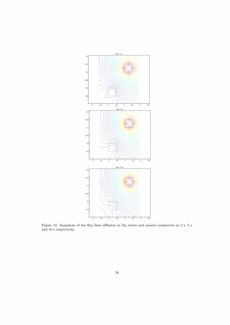
Figure 12: Snapshots of the flux lines diffusion in the active and passive conductors at 2 s, 5 sand 10 s respectively.

18

Table 3: Current densities 105A/m2 in the 5 points Ak of the active conductor.

t (s) A1 A2 A3 A4 A5

2FEFF

7.4367.437

6.4056.538

5.7665.746

5.5715.575

3.2843.279

5FEFF

11.8011.99

11.1811.48

9.96610.15

9.88310.09

8.6478.909

10FEFF

16.0016.40

15.9416.22

14.1014.50

14.1114.53

13.9514.36

Table 4: Current densities 105A/m2 in the 5 points Pk of the passive conductor.

t(s) P1 P2 P3 P4 P5

2FEFF

7.4367.437

1.1601.194

1.6851.754

1.8081.834

1.1011.131

5FEFF

2.0122.136

2.5082.634

2.4722.572

3.3543.443

2.3112.455

10FEFF

2.1622.269

2.4952.584

2.3782.455

2.8622.903

2.5442.675

proprieties can be different cell to cell. The sources can be easily modelled both in the case ofdiscontinuous and in the case of concentrated sources.

The results obtained in the case of an axisymmetric eddy currents problem proved to be in a goodagreement with those from the classical Finite Elements method, based on the differential approach.The implemented finite formulation approach can be extended to the 3D magnetic field analyses.

8 Acknowlegments

The author is greatful to Prof. E. Tonti and Dr. A. Bossavit for his helpful advices and suggestions.

References

[1] R. Albanese, G. Rubinacci, “Finite Element Method for the Solution of 3D Eddy Current Problems”,Advances in Imaging and Electron Physics, vol.102, pp.1–86, April 1998.

[2] F. Bellina, P. Bettini, E. Tonti, F. Trevisan, “Finite Formulation for the Solution of a 2D eddy currentproblem”, in printing on IEEE Transaction on Magnetics of March 2002.

[3] A. Bossavit, J.C. Verite, A Mixed FEM-BIEM Method to Solve Eddy-Currents Problems, IEEE Trans.,MAG-18 (1982) pp. 431-435.

[4] A. Bossavit, “A rationale for edge-elements in 3-D fields computations”, IEEE Trans. on Magnetics,Vol. 24, No. 1, 74-79, 1988.

[5] A. Bossavit, ”How Weak is the Weak Solution in Finite Element Methods?”, IEEE Trans. Mag. Vol.34, No. 5, Sep. 1998.

[6] A. Bossavit, “Computational Electromagnetism”, Academic Press, 1998.

19

[7] A. Bossavit, L. Kettunen ”Yee-like Schemes on Staggered Cellular Grids: A synthesis Between FIT andFEM Approaches”, Vol. 36, No. 4, July 2000.

[8] Tarhasaari, A. Bossavit, L. Kettunen ”Some Realization of a Discrete Hodge Operator: a Reinterpre-tation of finite Element Techniques”, IEEE Trans. Mag. 35, 3, 1998.

[9] M. Clemens, T. Weiland, “Transient Eddy Current Calculation with the FI-method”, IEEE trans. mag.vol. 35, pp. 1163-1165.

[10] E. Hallen, “Electromagnetic Theory”, Chapman & Hall, 1962.

[11] H. Penfield, H. Haus, “Electrodynamics of Moving Media”, M.I.T. Press, 1967.

[12] J. Stoer, R. Bulirsch, “Introduction to Numerical Analysis”, Springer-Verlag, N. Y. 1980.

[13] E. Tonti, “Finite Formulation of the Electromagnetic Field”, progress in Electromagnetics Research,PIER 32, pp. 1-44, 2001.

[14] E. Tonti, “On the Geometrical Structure of Electromagnetism”, in Gravitation, Electromagnetism andGeometrical Structures, for the 80th birthday of A. Lichnerowicz, Edited by G. Ferrarese. PitagoraEditrice Bologna, 1995, pp. 281—308.

[15] E. Tonti, “On the Formal Structure of Physical Theories”, preprint of the Italian National ResearchCouncil, 1975.

[16] E. Tonti, “The reasons for Analogies between Physical Theoriees”, Appl. Mat. Modelling, I, pp. 37-50,1976.

[17] E. Tonti, “Algebraic topology and computational electromagnetis”, in Proc. of 4th Int. Workshop onElectric and Magnetic Fields, Marseilles, France, 1998, pp. 285-294.

[18] T. Weiland, “On the Numerical Solution of Maxwell’s equations and applications in the field acceleratorphysics”, Particle Accelerators 245-292, 1984.

[19] K. S. Yee, “Numerical Solution of Initial Boundary Value Problems Involving Maxwell’s Equations inIsotropic Media”, IEEE Trans. on Antennas Propagation, 14, pp. 302-307, 1966.

[20] J. Rotman, ”An introduction to algebraic topology”, Springer-Verlag, 1988.

[21] W. Rudin, ”Principles of Mathematica Analysis”, McGraw-Hill, Inc., 1976.

[22] M. Marrone, ”Computational aspects of the Cell Method in Electrodynamics”, PIER 32, pp. 317-356,2002.

20